1 An improved model and a heuristic for capacitated lot sizing and scheduling in job shop problems O. Poursabzi 1 , M. Mohammadi* , 1 , B. Naderi 1 1 Department of Industrial Engineering, Faculty of Engineering, Kharazmi University, Tehran, Iran Email addresses: [email protected] (O. Poursabzi), [email protected] (M. Mohammadi), [email protected] (B. Naderi) Abstract This paper studies the problem of capacitated lot-sizing and scheduling in job shops with a carryover set- up and a general product structure. After analyzing the literature, the shortcomings are easily realized; for example, the available mathematical model is unfortunately not only non-linear but also incorrect. No lower bound and heuristic is developed for the problem. Therefore, we first develop a linear model for the problem on-hand. Then, we adapt an available lower bound in the literature to the problem studied here. Since the problem is NP-hard, a heuristics based on production shifting concept is also proposed. Numerical experiments are used to evaluate the proposed model and algorithm. The proposed heuristic is assessed by comparing it against other algorithms in the literature. The computational results demonstrate that our algorithm has an outstanding performance in solving the problem. Keywords: lot-sizing and scheduling; job shop; Sequence-Dependent; Lower bound; Heuristic. 1. Introduction Production management is a multi-disciplinary task simultaneously involving many factors. Lot-sizing and scheduling are the two main parts of production planning and control system. Lot-sizing deals with determining the production amount of each product at each production run, often over a finite multi- period horizon. A lot indicates the quantity of a given product processed on a machine continuously without interruption after its correspondent set-up. On the other hand, scheduling is to determine the production sequence in which the products are manufactured on a single machine [1]. The integrated problem provides a more effective production plan compared to the cases in which two problems are solved hierarchically by inducing the solution of the lot-sizing problem in the scheduling level. Simultaneous lot-sizing and scheduling is essential especially when sequence-dependent set-up costs and times occur [2]. In many of the production environments, switching between production lots of two different products triggers operations such as machine adjustments, tool changing and cleansing procedures. These set-up operations are usually dependent on the sequence [2]. In order to avoid

Welcome message from author
This document is posted to help you gain knowledge. Please leave a comment to let me know what you think about it! Share it to your friends and learn new things together.
Transcript
1
An improved model and a heuristic for capacitated
lot sizing and scheduling in job shop problems
O. Poursabzi1, M. Mohammadi*, 1, B. Naderi1
1Department of Industrial Engineering, Faculty of Engineering, Kharazmi University, Tehran, Iran
Email addresses: [email protected] (O. Poursabzi), [email protected] (M.
Mohammadi), [email protected] (B. Naderi)
Abstract
This paper studies the problem of capacitated lot-sizing and scheduling in job shops with a carryover set-
up and a general product structure. After analyzing the literature, the shortcomings are easily realized; for
example, the available mathematical model is unfortunately not only non-linear but also incorrect. No
lower bound and heuristic is developed for the problem. Therefore, we first develop a linear model for the
problem on-hand. Then, we adapt an available lower bound in the literature to the problem studied here.
Since the problem is NP-hard, a heuristics based on production shifting concept is also proposed.
Numerical experiments are used to evaluate the proposed model and algorithm. The proposed heuristic is
assessed by comparing it against other algorithms in the literature. The computational results demonstrate
that our algorithm has an outstanding performance in solving the problem.
Keywords: lot-sizing and scheduling; job shop; Sequence-Dependent; Lower bound; Heuristic.
1. Introduction
Production management is a multi-disciplinary task simultaneously involving many factors. Lot-sizing
and scheduling are the two main parts of production planning and control system. Lot-sizing deals with
determining the production amount of each product at each production run, often over a finite multi-
period horizon. A lot indicates the quantity of a given product processed on a machine continuously
without interruption after its correspondent set-up. On the other hand, scheduling is to determine the
production sequence in which the products are manufactured on a single machine [1].
The integrated problem provides a more effective production plan compared to the cases in which two
problems are solved hierarchically by inducing the solution of the lot-sizing problem in the scheduling
level. Simultaneous lot-sizing and scheduling is essential especially when sequence-dependent set-up
costs and times occur [2]. In many of the production environments, switching between production lots of
two different products triggers operations such as machine adjustments, tool changing and cleansing
procedures. These set-up operations are usually dependent on the sequence [2]. In order to avoid
2
unnecessary changeovers, customer demand has to be pooled in the production orders (lots). When
sequence-dependent set-up times are predominant, the available capacity for production depends on both
sequence and size of the lots. In such a situation, lot-sizing and scheduling have to be applied
simultaneously [3]. Consequently, the production sequence must be explicitly embedded in the lot
definition and scheduling.
The problem of the integrated lot-sizing and scheduling can be either capacitated or incapacitated [4].
Another issue in this area is the product structure. In one type, only a set of final products are planned,
while in another one, assembly products are assumed [2]. That is, each final product is the assembly of
some other intermediate products and it can be manufactured when all its intermediate products are
planned. In the assembly type, the products can either have serial or general structure. In the serial
structure, each product has only one predecessor and one successor, while in the general one, each
product can have multiple predecessors and successors. If each product needs one operation for
completion, the problem is called single-level while if it requires more than one operation, the problem is
defined as multi-level. In the case of the multi-level operation where all the products have the same
processing route, the problem is called a flow shop, while where each one has its own unique processing
route, the problem is called a job shop.
The incapacitated problem has been well studied in the literature. The incapacitated lot-sizing flow
shop is reviewed by Ouennicheh and Bertrand [5] while the incapacitated lot-sizing job shop is studied by
Ouenniche et al. [6]. Regrding the capacitated problems, the first conclusion is that the papers focus more
on the flow shops than the job shops. In this regard, one can refer to Maravelias and Sung [7], Karimi-
Nasab and Seyedhoseini [8], Stadtler and Sahling [9], and Babaei et al. [10].
Mohammadi et al. [11] considered the flow shop-based lot sizing and scheduling problem and
proposed a mixed integer linear programming (MILP) model. Their model was an extension of the model
previously proposed for the parallel-machine version of the flow shop-based lot sizing and scheduling
problem [12]. Later, the same authors proposed several rolling horizon heuristics in [11] and [13] and a
genetic algorithm (GA) was extended by Mohammadi et al. [14, 15] for the same problem. Mohammadi
and Jafari [16] also developed the mentioned problem with parallel machines at each stage. They
proposed a lower bound (LB) as well as a mixed integer programming-based algorithm. Ramezanian et al.
[17] developed an improved mathematical model for the same problem proposed by Mohammadi et al.
[15]. Ramezanian and Saidi-Mehrabad [18] developed the problem with stochastic processing times and
proposed a mixed integer programming (MIP) model.
Considering the importance of the lot-zing and scheduling of the job shop manufacturing systems,
this issue has less been studied compared to the flow shop systems. Hence, we will present a review on
this issue in the following.
Karimi-Nasab and Seyedhoseini [8] studied the job shop-based problem, but they ignored considering
carryover set-up times. More importantly, they also only considered scheduling of final products and
oversight the general product structure. Moreover, Fandel and Hegene [2] generalized the problem with
both carryover set-up and general product structure and proposed a mathematical model for the problem.
Unfortunately, this model does not work correctly. More detail on why the model is incorrect is presented
in Section 2. Besides its incorrectness, the model of Fandel & Stammen-Hegene [2] is non-linear. Authors
did not proposed solution method to solve the problem.
Lasserre [19] and Dauzere-Peres and Lasserre [20] presented integrated models of multi product,
multi periods, job shop lot sizing and scheduling problems considering set-up scheduling for the job shop
manufacturing system. Since this problem is NP-hard, they offered a decomposition approach in which on
3
a production planning problem with a fixed sequence of products on machines is considered at first and
then, based on this fixed production plan, the scheduling is determined using an adapted version of
Shifting Bottleneck algorithm.
Lalitha et al. [21] studied N-stage hybrid flow shop lot streaming problem for the multi products,
single period case. The aim was to minimize the makespan. In this regard, they tried to respond to the
following issues: quantity of sub-lots, sequence of sub-lots and jobs. Since the problem is NP-hard, they
developed a heuristic algorithm for large scale instances. Giglio et al. [22] studied a lot-sizing and
scheduling problem considering energy consumption with the goal of minimizing total cost of the system.
Their solved a single-level and multi period problem and considered fixed set-up parameters. They also
implemented a relax-and-fix based heuristic algorithm. Wolosewicz et al. [23] considered a constant
sequence for the operations in the lot-sizing and scheduling problem with the constant set-up. They
developed an adaptation of Lagrangian methods for the large scale instances. Karimi-Nasab et al. [24]
considered a lot-sizing and scheduling problem with compressible processing time. They considered a
constant sequence of jobs where by allocating the jobs to each machine, the lot size of jobs would be
determined. Also, their solution procedure was a variation of Particle Swarm Optimization (PSO).
Karimi-Nasab and Modarres [25] investigated simultaneous lot-sizing and scheduling problem in a job
shop manufacturing environment over a finite number of periods. They supposed that each machine can
operate at different discrete speed levels, and the set of modes for each machine is known in advance. The
problem was formulated as an integer linear program (ILP) and a branch and cut approach was then
employed so as to solve it. The goal was to minimize the total costs originated from set-up, production,
inventory holding, and shortage. Urrutia et al. [26] incorporated both lot-sizing and scheduling problems
simultaneously and considered sequence independent set-up time/cost, single level and multi items. In
order to solve the problem, they considered a constant sequence of jobs and solved their models using an
adaptation of Lagrangian method. They made an endeavor to solve the lot-sizing problem at first and then
tried to improve the sequence of jobs. Mateus et al. [27] studied a constrained lot-sizing and scheduling
problem under single level manufacturing system, unrelated parallel machines and sequence dependent
set-ups conditions. They optimized their solution as separable (independent) consequent processes. First,
lot sizes were calculated and then the scheduling problem was solved using GRASP method. Finally, a
new methodology was presented so as to combine both solutions together. Zhang and Yang [28] proposed
a non-linear mathematical model for the multi products, multi periods simultaneous lot-sizing and
scheduling problem where the type of set-up was simple and only end products were taken into account.
They also deployed a GA to solve the problem on hand. Ouenniche and Bactor [29] proposed a multi-
stage approach to find a solution for the lot-sizing and scheduling problem. They first determined the
scheduling by solving a non-linear model and then lot sizes were calculated based on the given schedules.
For the medium and large scale problems, they implemented Simulated Annealing (SA) and Tabu Search
(TS) algorithms. In their model, the demand of customers was deterministic and set-ups were independent
from sequences.
After a detailed review of the literature, the existing research gap motivated the authors to study the
problem of job shop-based lot-sizing and scheduling so as to overcome the current shortcomings of the
literature. This paper first presents a mixed integer, interestingly linear, programming model and both the
problem and the model is then analyzed to introduce an effective LB. Moreover, a production shifting-
based heuristic is proposed so as to solve the problem. The proposed model, LB and heuristics are
evaluated through several numerical experiments.
4
The rest of the paper is organized as follows: Section 2 defines and formulates the problem on hand.
Section 3 presents the proposed LB while Section 4 proposes a production shifting-based heuristic. Then,
Section 5 conducts numerical experiments to evaluate the proposed model, LB and heuristics. Finally,
Section 6 provides conclusions and future research directions.
2. The problem definition and formulation
The problem under consideration can be described as follows. There is a set of N products and a set
of M machines for production. On the one hand, the products are assumed to follow the general product
structure (i.e., they are assembly products where each part might have more than one predecessor and
successor). The lower level products are the elements of the higher level ones. Therefore, the production
of the upper levels can be started when all of its elements at the lower levels are already produced. Also,
the products are assumed to be multi-level; that is, each product needs multiple operations for completion.
Each operation is carried out with one machine where the processing route of each product differs from
the others. Note that one operation can be started when its precedent operation is already finished, called
vertical interaction.
The planning horizon is finite consisting of T macro-periods of the same length. For each product,
there may be both external (independent) and internal (dependent) demands. The final products have only
external demands. The demands for each period have to be satisfied during that period. Thus, no shortage
is allowed. Moreover, each product can be produced at most as a single lot during each period.
In this production system, we assume that machines are capacitated as resources. The set-up is also
assumed to be sequence-dependent (i.e., its magnitude and cost depend on product sequence) and carry-
over (i.e., it can be accomplished within the next micro period). Each macro period is segmented into
several micro periods (see Figure 1) where the first micro period is also assigned for set-up process.
Regarding the precedence relations and the general product structure, some standstills may occur during
the process where their length can be measured using the shadow product concept. Each product cannot
be produced on more than one machine in a micro period and also each machine cannot process more
than one product in a micro period. It is also assumed that machines are continuously available.
The integrated lot-sizing and scheduling problem is concerned with determining the periods in which
all products are manufactured, their lot size as well as product sequence on each machine, simultaneously.
The objective is to minimize the cost of the network including set-up, production, inventory and idle
costs.
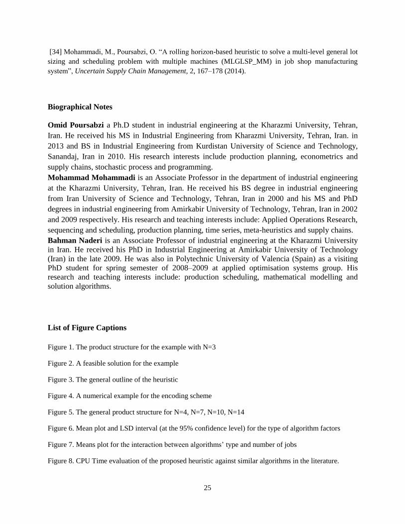
For further illustration, a numerical example is presented. Consider a job shop problem with three
products and two machines including the two planning horizons and two macro periods. Figure 1 and
Table 1 show the three product structures and demands, respectively. The processing route is as follows:
Product 1= {1,2}, Product 2= {2,1}, and Product 3= {2}
Please Insert Figure 1
Please Insert Table 1
5
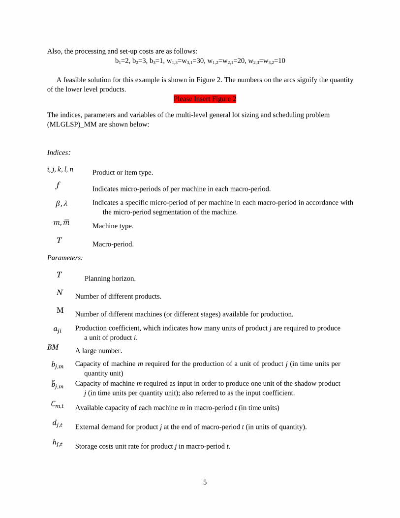
Also, the processing and set-up costs are as follows:
b1=2, b2=3, b3=1, w1,3=w3,1=30, w1,2=w2,1=20, w2,3=w3,2=10
A feasible solution for this example is shown in Figure 2. The numbers on the arcs signify the quantity
of the lower level products.
Please Insert Figure 2
The indices, parameters and variables of the multi-level general lot sizing and scheduling problem
(MLGLSP)_MM are shown below:
Indices:
i, j, k, l, n Product or item type.
f Indicates micro-periods of per machine in each macro-period.
Indicates a specific micro-period of per machine in each macro-period in accordance with
the micro-period segmentation of the machine.
Machine type.
T Macro-period.
Parameters:
T Planning horizon.
N Number of different products.
M Number of different machines (or different stages) available for production.
Production coefficient, which indicates how many units of product j are required to produce
a unit of product i.
BM A large number.
Capacity of machine m required for the production of a unit of product j (in time units per
quantity unit)
Capacity of machine m required as input in order to produce one unit of the shadow product
j (in time units per quantity unit); also referred to as the input coefficient.
Available capacity of each machine m in macro-period t (in time units)
External demand for product j at the end of macro-period t (in units of quantity).
Storage costs unit rate for product j in macro-period t.
6
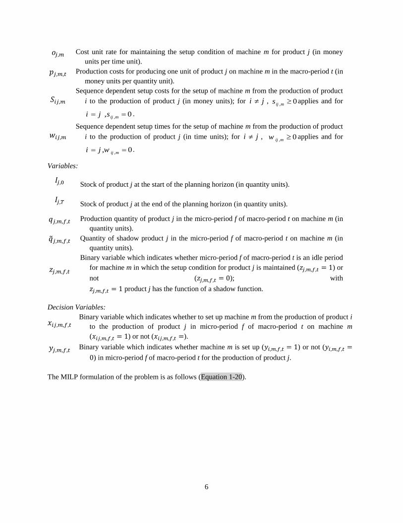
Cost unit rate for maintaining the setup condition of machine m for product j (in money
units per time unit).
Production costs for producing one unit of product j on machine m in the macro-period t (in
money units per quantity unit).
Sequence dependent setup costs for the setup of machine m from the production of product
i to the production of product j (in money units); for i j , , 0ij ms applies and for
, , 0ij mi j s .
Sequence dependent setup times for the setup of machine m from the production of product
i to the production of product j (in time units); for i j , , 0ij mw applies and for
,, 0ij mi j w .
Variables:
Stock of product j at the start of the planning horizon (in quantity units).
Stock of product j at the end of the planning horizon (in quantity units).
Production quantity of product j in the micro-period f of macro-period t on machine m (in
quantity units).
Quantity of shadow product j in the micro-period f of macro-period t on machine m (in
quantity units).
Binary variable which indicates whether micro-period f of macro-period t is an idle period
for machine m in which the setup condition for product j is maintained ( ) or
not ( ); with
product j has the function of a shadow function.
Decision Variables:
Binary variable which indicates whether to set up machine m from the production of product i
to the production of product j in micro-period f of macro-period t on machine m
( ) or not ( ).
Binary variable which indicates whether machine m is set up ( ) or not (
) in micro-period f of macro-period t for the production of product j.
The MILP formulation of the problem is as follows (Equation 1-20).
7
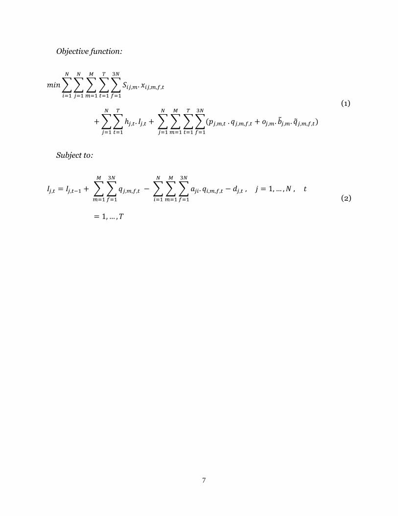
Objective function:
∑∑ ∑ ∑∑
∑∑ ∑ ∑ ∑∑
(1)
Subject to:
∑ ∑
∑ ∑ ∑
(2)
8
[ ] [ ( )
* ∑ ∑
∑
+]
[ ] * ( )
∑ ∑( ∑
)+
(3)
∑∑
∑∑∑
∑∑
(4)
(5)
(6)
9
∑
(7)
∑
(8)
∑
(
∑
)
(9)
(10)
∑
(11)
( )
(12)
( )
(13)
(∑∑
)
(14)
10
∑∑
(15)
(16)
{ } (17)
{ } (18)
{ } (19)
(20)
In this model, Equation 1 represents the objective function which minimizes the sum of the sequence-
dependent set-up costs, the storage costs, the production costs and the costs of maintaining the machine’s
set-up conditions in the planning horizon. Constraint 2 ensures the balance of demand supply in each
period. Two types of product's demand are taken into account in this model: 1) the external demand for
products that must be provided at the end of each macro-period, 2) the internal demand of the products
required for the production of high-level products in the product structure which must be satisfied within
the macro-period. The external demand ( ) and the internal demand (∑ ∑ ∑
) of a
macro-period for the product j must be provided by previous macro-period’s stock and the production
quantity of product j in current macro-period. Here, the first period is exception, since the demands have
to be provided by production.
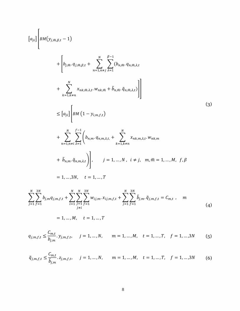
Constraint 3 is used so as to consider vertical interaction in the proposed model. In this equation, each
typical product is produced before its direct substitute product in one macro-period. The left side of
constraint 3 is equal to the time between the beginning of the macro-period t and the end of the
production of product j if micro-period f is a production micro-period for product j; otherwise, it is zero.
In other words, if the value is not positive, the left side of constraint 3 becomes zero. The right side of
constraint 3 is equal to the time between the beginning of period t and the beginning of the production of
product i if micro-period f is a production micro-period for product i, else it is a big number. In other
words, if the value is positive, the right side of constraint 3 is zero.
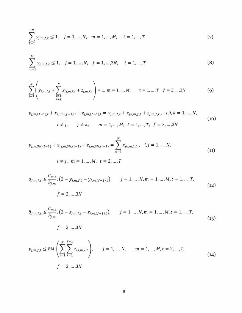
Constraint 4 shows the capacity constraints of machines during a macro-period. Constraint 5 indicates
the relation between set-up and production processes and obtains an upper bound (UB) for production
quantity. Constraint 6 determines the duration of idle times. It also yields a UB for the duration of the idle
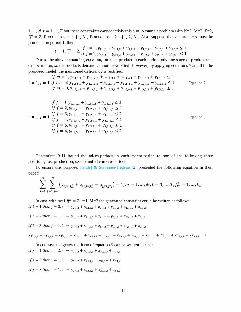
times. Constraints 7 and 8 guarantee that in each macro-period, at most a single lot is produced for each
product. To achieve this aim, Fandel & Stammen-Hegene [2] applied ∑ ∑
11
but these constraints cannot satisfy this aim. Assume a problem with N=2, M=3, T=2,
, Product_rout{1}={1, 3}, Product_rout{2}={1, 2, 3}. Also suppose that all products must be
produced in period 1, then:
Due to the above expanding equation, for each product in each period only one stage of product rout
can be run on, so the products demand cannot be satisfied. However, by applying equations 7 and 8 in the
proposed model, the mentioned deficiency is rectified.
Equation 7
Equation 8
Constraints 9-11 bound the micro-periods in each macro-period to one of the following three
positions; i.e., production, set-up and idle micro-period. To ensure this purpose, Fandel & Stammen-Hegene [2] presented the following equation in their
paper:
∑ ∑ (
)
In case with m=1, , t=1, M=3 the generated constraint could be written as follows:
In contrast, the generated form of equation 9 can be written like so:
12
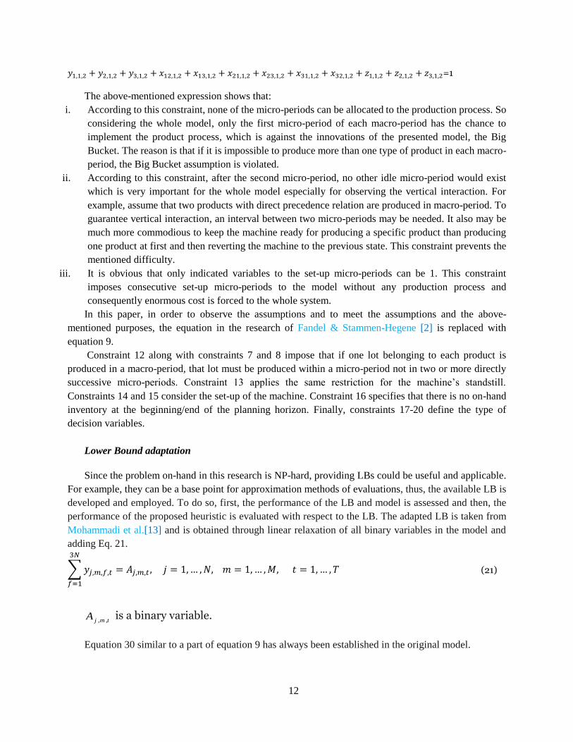
=1
The above-mentioned expression shows that:
i. According to this constraint, none of the micro-periods can be allocated to the production process. So
considering the whole model, only the first micro-period of each macro-period has the chance to
implement the product process, which is against the innovations of the presented model, the Big
Bucket. The reason is that if it is impossible to produce more than one type of product in each macro-
period, the Big Bucket assumption is violated.
ii. According to this constraint, after the second micro-period, no other idle micro-period would exist
which is very important for the whole model especially for observing the vertical interaction. For
example, assume that two products with direct precedence relation are produced in macro-period. To
guarantee vertical interaction, an interval between two micro-periods may be needed. It also may be
much more commodious to keep the machine ready for producing a specific product than producing
one product at first and then reverting the machine to the previous state. This constraint prevents the
mentioned difficulty.
iii. It is obvious that only indicated variables to the set-up micro-periods can be 1. This constraint
imposes consecutive set-up micro-periods to the model without any production process and
consequently enormous cost is forced to the whole system.
In this paper, in order to observe the assumptions and to meet the assumptions and the above-
mentioned purposes, the equation in the research of Fandel & Stammen-Hegene [2] is replaced with
equation 9.
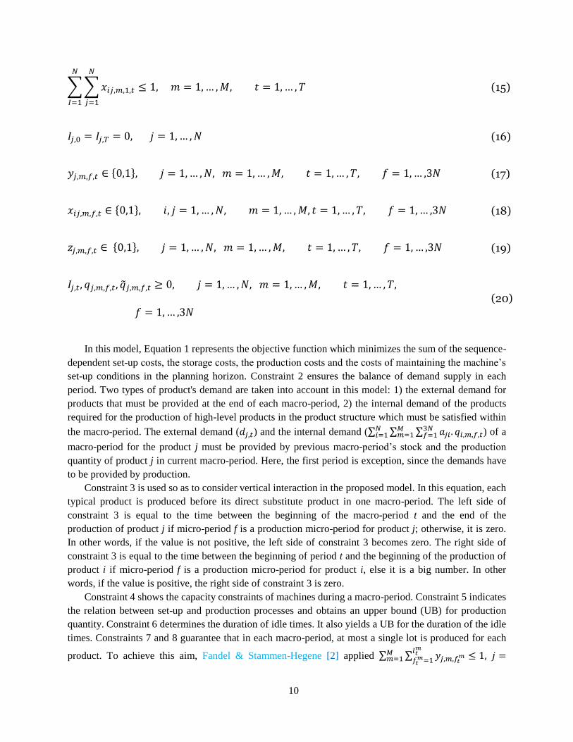
Constraint 12 along with constraints 7 and 8 impose that if one lot belonging to each product is
produced in a macro-period, that lot must be produced within a micro-period not in two or more directly
successive micro-periods. Constraint 13 applies the same restriction for the machine’s standstill.
Constraints 14 and 15 consider the set-up of the machine. Constraint 16 specifies that there is no on-hand
inventory at the beginning/end of the planning horizon. Finally, constraints 17-20 define the type of
decision variables.
Lower Bound adaptation
Since the problem on-hand in this research is NP-hard, providing LBs could be useful and applicable.
For example, they can be a base point for approximation methods of evaluations, thus, the available LB is
developed and employed. To do so, first, the performance of the LB and model is assessed and then, the
performance of the proposed heuristic is evaluated with respect to the LB. The adapted LB is taken from
Mohammadi et al.[13] and is obtained through linear relaxation of all binary variables in the model and
adding Eq. 21.
∑
(21)
, ,j m tA is a binary variable.
Equation 30 similar to a part of equation 9 has always been established in the original model.
13
After relaxing the binary variables, neither equation 3 nor 14 has no significant influence on the
model, since the left side of equation 3 would be a big negative number and the right side of equation 3 or
14 would be a big positive number owing to the values of the relaxed variables . It means that by
relaxing the binary variables, equation 3 or 14 is always satisfied without imposing any obligation so as to
guarantee vertical interaction in the model. Thus, in calculating of the LB, equation 3 or 14 can be
eliminated from the model.
3. The proposed Shifting-Based heuristic
Since the problem on hand is NP-hard, it cannot be solved in a reasonable computational time using
the exact classical methods. To rectify such a difficulty, employing heuristics is the best alternative [30].
The proposed heuristic in this research is based on part (or entire) of product lot shifting from a specific
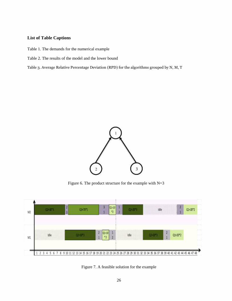
period to others and includes 4 phases: initializing, smoothing, improving and merging mechanisms.
In initializing mechanism, an initial solution is generated through ignoring the capacity constraints. If
this initial solution is infeasible, the smoothing mechanism is used to obtain a feasible solution based on
the concept of product shifting. The improving mechanism starts from the obtained feasible solution of the
smoothing mechanism and try to improve this solution. In merging mechanism phase, the produced lots
obtained from improving procedure are integrated with the goal of reducing the set-up cost. If, the
solution obtained from the merging mechanism phase is infeasible, it will be used as the initial solution of
the next iteration.
The algorithm repeats until the stopping criterion is met. The general outline of the proposed heuristic
is shown in Figure 3. The 4 mechanisms are described as follows.
Please Insert Figure 3
3.1. Initialization
In this mechanism, one initial solution is generated. It should be noted that three decisions should be
made in the problem under consideration: products to be produced at each period, the lot-size of each
product and product sequence on each machine. Obviously, these decisions are determined in any
solution. The used heuristic search in this research defines the first two decisions and tries to improve
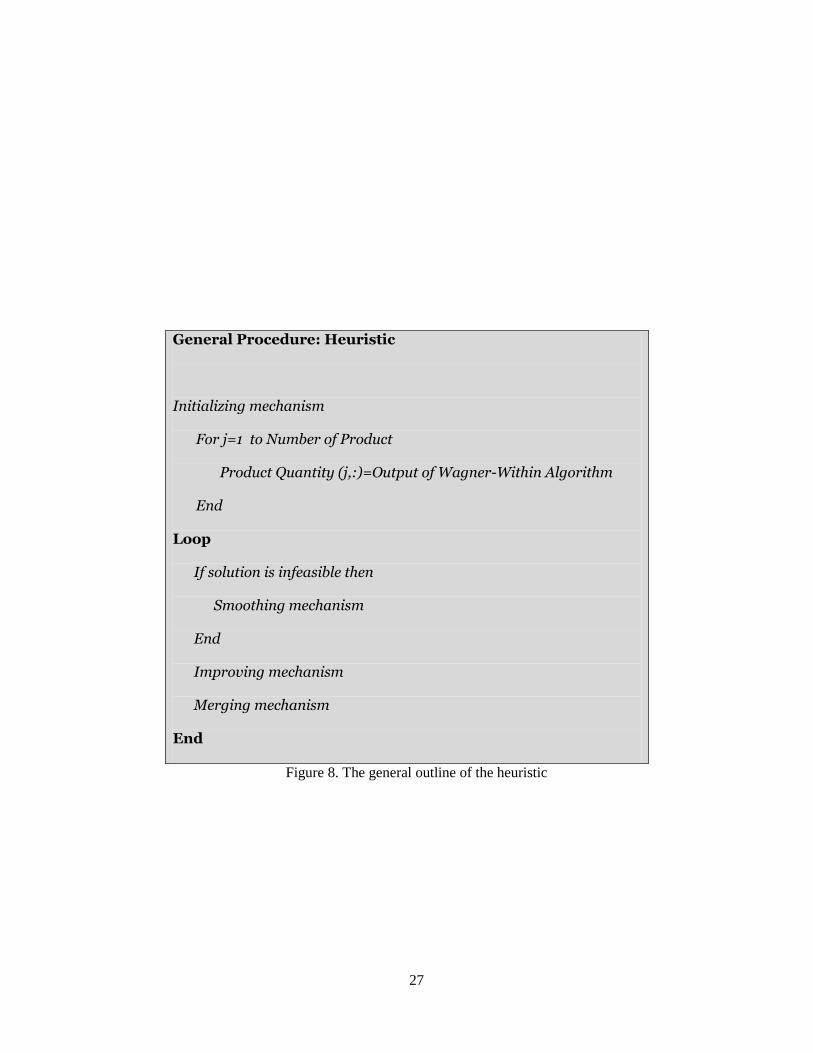
them while the product sequence of a given solution is defined using a dispatching rule. Figure 4 shows
how a solution is encoded in the proposed heuristic in terms of a numerical example.
Please Insert Figure 4
{
First, the initial solution is generated for the incapacitated version of the problem. This solution is then
becomes feasible using the soothing mechanism, if it violates the capacity constraint. To this end,
Wagner-Whitin algorithm is used for each product. The algorithm is first applied to items with
independent demand dj,t. It is then applied to each item 2,...,j N with both independent and
dependent demands.
Those products should be produced during the studied period according to the encoding scheme must
have the following conditions. Let P(j) be a set including all products that can be produced i.e., there is
14
sufficient amount of its prerequisites. The sequence can be determined considering the following rules
among those products which have necessary conditions for production. In each step, the products in
which the examined machine is one of the production process steps, are selected. At the beginning steps
of production, if a given product has any prerequisite then a required amount of necessary materials
should be available in order to make sure that the product is considered as a candidate for the operation.
Also, if the examined machine is in any step except the first step then the operation on the product should
be completed in previous steps. Due to [2], those products in lower levels of general product structure
(GPS), have a greater number of demands and also there are many products which are dependent on these
mentioned products for initiating their production process; therefore, they are assigned higher priority for
production.
If there is more than one output from the previous level, the High priority product is the one with
lower average set-up cost. The average set-up cost for product j on machine m is derived from ∑
∑ ∑ . If the examined product is the first produced product of the considered machine during the
current macro-period, its set-up could be performed in previous period(s) by concerning cost and source.
In this case, the carryover option for set-up should be applied to the next period.
A well-known property, called zero-switch property [31], for the incapacitated lot-sizing problem can
be defined as follows: there is an optimal solution for the incapacitated lot-sizing problem (the problem
GCLSP without resource constraints) where one can write
Product quantity(j,t)*Inventory(j,t-1)=0
or
(∑ ∑
) (∑ ∑
)
Using this property, the production quantity of each item in its production periods can be calculated as
such.
Step 1: For any item j and period t, if Ej,t=0 then set Product quantity(j,t)=0
Step 2: For any item j any periods t1<t2≤T, if Ej,t1=Ej,t2 =1 and Ej,t=0 for all t1<t<t2 then
∑ ( ∑
)
(22)
In other words, if a product is produced in a given period, the demand of that period as well as all
periods up to the next production period of that item should be satisfied. Since no backlogging is
assumed, all items are produced in the first period, i.e.:
.
In CLSP, the optimal solution may do not include zero-switch property, since it also depends on the
available capacity of machines. Hence, the solution, derived from this property, is used as a base solution
to generate a feasible solution considering capacity constraints. This procedure is carried out using a
heuristic explained in the next subsection.
3.2. Smoothing mechanism
The initial solution (P1) may be infeasible owing to violating capacity constraint. In this case, the
smoothing mechanism aims to generate a feasible solution named P2 through shifting products from an
infeasible period to other periods. Note that a period is infeasible if the capacity constraint is violated.
15
In an infeasible period t, a portion of product quantity named qit out of total production quantity of
item j in period t is transferred to another period tl. For each item j produced in an infeasible period t, two
quantities are considered to shift to period tl:
Wj,tl: The maximum production quantity of product j in period t; which guarantees that inventory
constraints are still satisfied. This amount depends on whether tl > t or tl < t.
Qj,t: The quantity of production j in infeasible period t: it eliminates the resource overload (machine
capacity) m in period t by shifting this quantity to another;
,(∑
∑ ∑
∑
)
⁄ - (23)
In Eq (23), the comparison is made only for positive values. Note that the amount Qi,t indicates that
overuse of resource k in the period t could be reduced to zero if there is a quantity less than Wi,tl,. The
smoothing mechanism includes the following two steps.
3.2.1. Backward shifts
In this mechanism, the production shifting from each period to earlier periods is analyzed. The
procedure starts from the last period and continuous toward the first period. If the period is infeasible, a
portion of selected produced product is moved to earlier periods so that period t becomes feasible. It
should be pointed out that the production shifting process is checked to all earlier periods and the best one
is selected. The product is also selected by the ratio test which will be discussed later. If no feasible
solution is found by shifting the first selected product, the procedure applies to the next product. For an
infeasible period t, a quantity Qj,t out of the entire production amount of product j in period t is shifted to
earlier target period tl where τ ≤ tl ≤ t-1. Note that we have
τ = max{1, the last period among periods prior to period t in which component j is produced}.
The production shifting increases the product stock in a period. In order to meet the inventory balance
constraints, the portion of the shifting must be held:
,
{
⁄ } - (24)
It is noteworthy to indicate that there always exists a component r whose entire production can be
moved to an earlier period, { | }, since
, where P(r) is the set of all immediate predecessors of component r. In other words,
the entire product of an item can be moved from the current period to earlier periods when none of its
components is produced in the current period.
The selection of quantity, component and target period (qj,t, j ,tl) is based on the ratio test derived from
cost variation calculation and resource usage. If the procedure continues to the first period and no feasible
solution is found, the forward shifting is applied. Otherwise, procedure P2 terminates.
16
3.2.2. Forward shifts
This mechanism deals with the production shifting from a given period to later periods. It starts from
the first period to the last and intends to shift a portion of a product to subsequent periods so as to make it
feasible. Similar to the backward shift, the production shift to all earlier periods is checked and the best
one is selected. The products are selected one by one and the procedure applies to the next product if no
feasible solution is found.
For an infeasible period t, a quantity qj,t out of the entire production amount of product j in period t is
shifted to later target period tl, where t+1 ≤ tl ≤ τ and τ = min{T, the first period among periods
subsequent to period t in which component j is produced}.
Similar to backward shifts, the selection of quantity, moved component and target period are also
based on the ratio test. The production shift to the next periods reduces the inventory from period t to tl-1;
therefore, the inventory balance should be guaranteed. Eq. (25) is used to determine the shifted quantity to
the next periods.
{ } (25)
After these shifting, if a feasible solution is found, P2 terminates, otherwise, the backward shift
procedure should be applied again.
3.2.3. Ratio test
This procedure aims at selecting the shifted quantity, component and target period (qj,t, j, tl ), i.e., the
quantity qj,t out of the entire production amount of component j in period t should be moved to an earlier
or later target period tl. The values of (qj,t, j, tl) are chosen so that the following ratio (Eq. (26)) is
minimized.
(26)
The Extra Cost (Eq. (27)) is calculated as follows:
(27)
By shifting qj,t from period t to tl , the cost variation calculated by Additional Cost (Eq. (28)) is
imposed.
*( ) (∑( ∑
)
)+ (28)
The first term of the right hand side of Eq. (28) calculates the production cost variation. The second
and third terms compute the inventory cost variation and set-up cost variation, respectively. Total Cost is
the current system costs which is derived from the model objective function. The Additional cost
parameters can be expressed as follows.
{
}
17
{
}
{
}
{
}
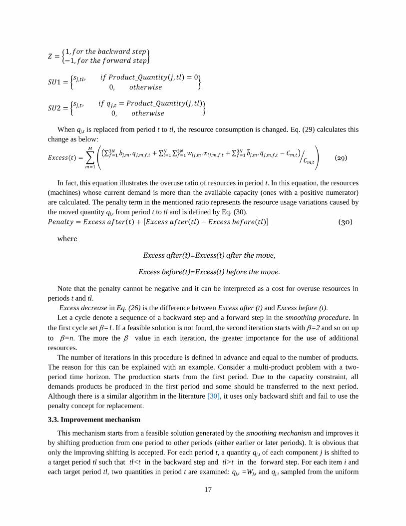
When qj,t is replaced from period t to tl, the resource consumption is changed. Eq. (29) calculates this
change as below:
∑ ((∑
∑ ∑
∑
)
⁄ )
(29)
In fact, this equation illustrates the overuse ratio of resources in period t. In this equation, the resources
(machines) whose current demand is more than the available capacity (ones with a positive numerator)
are calculated. The penalty term in the mentioned ratio represents the resource usage variations caused by
the moved quantity qj,t from period t to tl and is defined by Eq. (30).
[ ] (30)
where
Excess after(t)=Excess(t) after the move,
Excess before(t)=Excess(t) before the move.
Note that the penalty cannot be negative and it can be interpreted as a cost for overuse resources in
periods t and tl.
Excess decrease in Eq. (26) is the difference between Excess after (t) and Excess before (t).
Let a cycle denote a sequence of a backward step and a forward step in the smoothing procedure. In
the first cycle set =1. If a feasible solution is not found, the second iteration starts with =2 and so on up
to =n. The more the value in each iteration, the greater importance for the use of additional
resources.
The number of iterations in this procedure is defined in advance and equal to the number of products.
The reason for this can be explained with an example. Consider a multi-product problem with a two-
period time horizon. The production starts from the first period. Due to the capacity constraint, all
demands products be produced in the first period and some should be transferred to the next period.
Although there is a similar algorithm in the literature [30], it uses only backward shift and fail to use the
penalty concept for replacement.
3.3. Improvement mechanism
This mechanism starts from a feasible solution generated by the smoothing mechanism and improves it
by shifting production from one period to other periods (either earlier or later periods). It is obvious that
only the improving shifting is accepted. For each period t, a quantity qj,t of each component j is shifted to
a target period tl such that tl<t in the backward step and tl>t in the forward step. For each item i and
each target period tl, two quantities in period t are examined: qj,t =Wj,t and qj,t sampled from the uniform
18
distribution U[0, wi,tl]. One reason for selection of the second random value is that different solutions may
be obtained with the same initial point. Moreover, the costs vary over time and shifting a quantity qjt <
wi,tl may result in a lower cost. Any candidate set (q,i,tl) in period t among all candidates which minimizes
the Extra cost is chosen. The procedure terminates when no feasible and improving solution is found.
3.4. Merging procedure
The purpose of this procedure is to further diversify the search. In this procedure, the entire production
of an item j in a given period is moved to another period tl (either earlier or later) in which that item is
produced. The aim of production lots merging is to reduce the set-up and production cost. The item
production process can be shifted to period tl if this item’s lot in the current period is equal to Wj,tl which
is calculated by Eq. (24) for tl<t, and by Eq.(25) for tl>t. If the obtained solution is feasible, the
improvement procedure (P3) is applied to enhance the solution’s quality. Otherwise, the obtained solution
is used as a new starting point for the Smoothing procedure (P2).
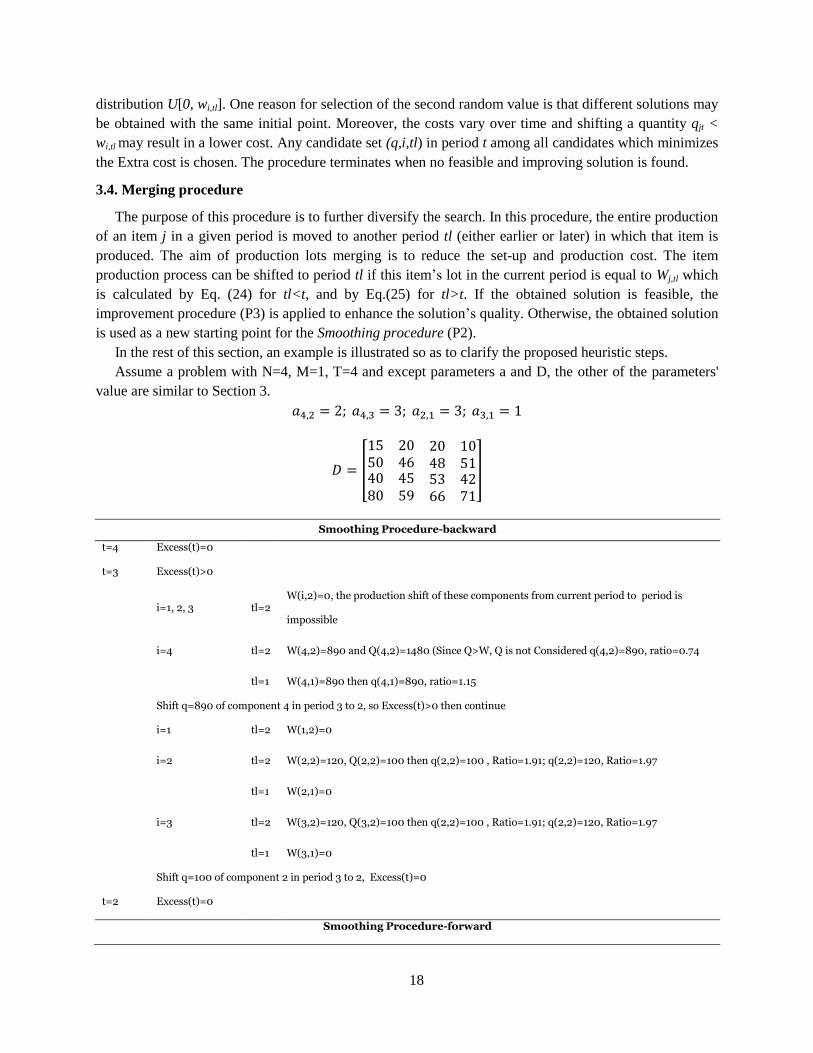
In the rest of this section, an example is illustrated so as to clarify the proposed heuristic steps.
Assume a problem with N=4, M=1, T=4 and except parameters a and D, the other of the parameters'
value are similar to Section 3.
[
]
Smoothing Procedure-backward
t=4 Excess(t)=0
t=3 Excess(t)>0
i=1, 2, 3 tl=2 W(i,2)=0, the production shift of these components from current period to period is
impossible
i=4 tl=2 W(4,2)=890 and Q(4,2)=1480 (Since Q>W, Q is not Considered q(4,2)=890, ratio=0.74
tl=1 W(4,1)=890 then q(4,1)=890, ratio=1.15
Shift q=890 of component 4 in period 3 to 2, so Excess(t)>0 then continue
i=1 tl=2 W(1,2)=0
i=2 tl=2 W(2,2)=120, Q(2,2)=100 then q(2,2)=100 , Ratio=1.91; q(2,2)=120, Ratio=1.97
tl=1 W(2,1)=0
i=3 tl=2 W(3,2)=120, Q(3,2)=100 then q(2,2)=100 , Ratio=1.91; q(2,2)=120, Ratio=1.97
tl=1 W(3,1)=0
Shift q=100 of component 2 in period 3 to 2, Excess(t)=0
t=2 Excess(t)=0
Smoothing Procedure-forward
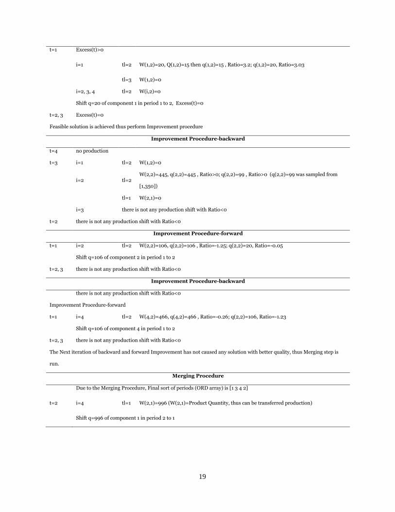
19
t=1 Excess(t)>0
i=1 tl=2 W(1,2)=20, Q(1,2)=15 then q(1,2)=15 , Ratio=3.2; q(1,2)=20, Ratio=3.03
tl=3 W(1,2)=0
i=2, 3, 4 tl=2 W(i,2)=0
Shift q=20 of component 1 in period 1 to 2, Excess(t)=0
t=2, 3 Excess(t)=0
Feasible solution is achieved thus perform Improvement procedure
Improvement Procedure-backward
t=4 no production
t=3 i=1 tl=2 W(1,2)=0
i=2 tl=2 W(2,2)=445, q(2,2)=445 , Ratio>0; q(2,2)=99 , Ratio>0 (q(2,2)=99 was sampled from
[1,350])
tl=1 W(2,1)=0
i=3 there is not any production shift with Ratio<0
t=2 there is not any production shift with Ratio<0
Improvement Procedure-forward
t=1 i=2 tl=2 W(2,2)=106, q(2,2)=106 , Ratio=-1.25; q(2,2)=20, Ratio=-0.05
Shift q=106 of component 2 in period 1 to 2
t=2, 3 there is not any production shift with Ratio<0
Improvement Procedure-backward
there is not any production shift with Ratio<0
Improvement Procedure-forward
t=1 i=4 tl=2 W(4,2)=466, q(4,2)=466 , Ratio=-0.26; q(2,2)=106, Ratio=-1.23
Shift q=106 of component 4 in period 1 to 2
t=2, 3 there is not any production shift with Ratio<0
The Next iteration of backward and forward Improvement has not caused any solution with better quality, thus Merging step is
run.
Merging Procedure
Due to the Merging Procedure, Final sort of periods (ORD array) is [1 3 4 2]
t=2 i=4 tl=1 W(2,1)=996 (W(2,1)=Product Quantity, thus can be transferred production)
Shift q=996 of component 1 in period 2 to 1
20
The algorithm terminates when maximum iteration number (MaxIT) or Max Run Time reach. The
optimum level selection of the algorithm’s max iteration is a serious challenge. In this regard, three levels
of the mentioned parameters are defined as 15, 20 and 25.
For the calibration of the algorithm, several problems are generated and solved, which ultimately 20 is
selected as the optimum level of Max iteration. Also, Max Run Time is set as 10,000 seconds.
4. The heuristic evaluation
In this section, the performance of the adapted LB and the proposed algorithm is evaluated. To this
end, the adapted LB is compared with the optimum solution in very small sized problems. Also the
proposed algorithm is compared with other algorithms as well.
The model is coded in LINGO 8 and the heuristic is implemented in MATLAB 2011a. All the
experiments are run on a PC with a 3.4 GHz Intel® Core™ 2 Duo processor and 4 GB RAM memory.
4.1. Evaluation of the model and Lower bound
In order to ensure the accuracy of the LB, a set of 15 instances similar to those used in Mohammadi et
al.[13] are generated as follows.
|
The capacity of each machine at each period denoted by is calculated so as to satisfy the demand
of that period according to the lot-for-lot (L4L) scenarios.
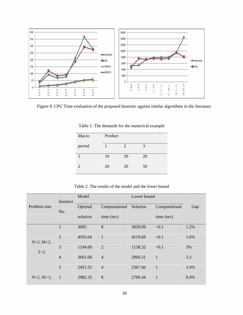
Table 2 shows the results of all instances belonging to the problem with [N=2, M=2, T=2] and [N=2,
M=3, T=2]. In Table 2, the first row shows the optimal solutions while the second row indicates the
difference between the LB and the optimal solution. Also the computational times in second are shown in
the third row.
The following performance measure (Eq. (31)) shows the gap, i.e., the difference between LB and the
optimal solution.
∑(
)
(31)
Where LBsolution,i is the solution obtained by the LB and GOsolution,i is the global optimum of
any instance.
The computational time for a problem with [N=2, M=2, T=2] and [N=2, M=3, T=2] are 5.2 and 42.2
seconds, respectively. It first reveals that the average computational time grows more than 8 times by
increasing only one machine to the system.
Please Insert Table 2
4.2. Heuristic evaluation
This subsection evaluates the performance of the presented heuristic. To do so, the output of the
applied algorithms for similar problems with the developed heuristic in this paper is compared. A set of
21
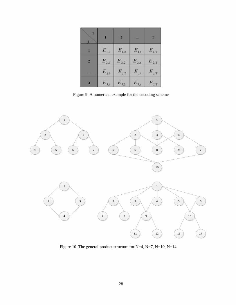
15 problems with different sizes from (N _ M _ T) = (3 _ 3 _ 3) to (14 _ 14 _ 14) are generated. The used
GPSs in the paper are shown in Figure 5. The test instances are taken from the literature [32] and [33].
These data sets can be divided into three groups:
1. Small-size including instances with sizes of 3.3.3 to 4.5.4,
2. Medium-size including instances with sizes of 7.5.5 to 7.7.7,
3. Large-size including instances with sizes of 10.7.7 to 14.14.14.
4. Please Insert Figure 5
Cm,t is also calculated so that the demand of each period according to the L4L scenarios is met [34].
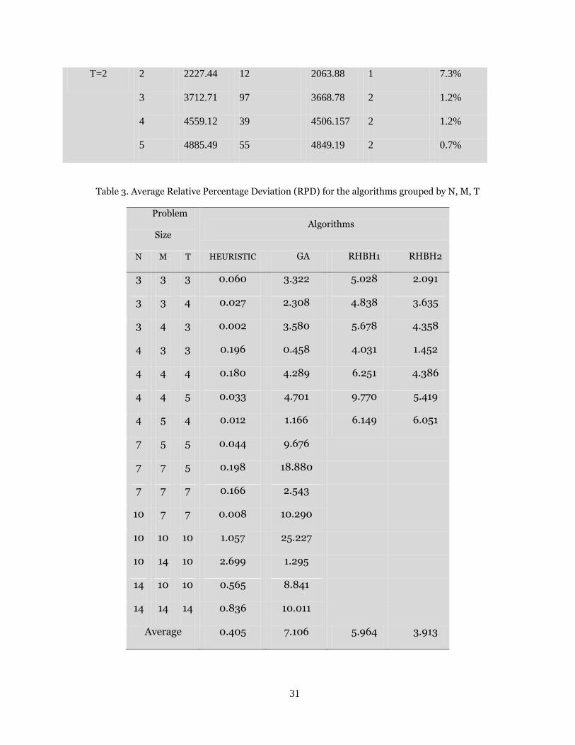
Table 3 shows the experiment results in which any instance is solved 5 times and its results are
normalized through using relative percentage deviation (RPD) metric calculated as follows (Eq. (32)):
(32)
Where is the relative percentage deviation of the jth instance of the i
th trial. Also, is the
objective function value obtained from the jth instance of the i
th trial and is a minimum value of the
objective function obtained for jth instance.
The average values of RPDs are shown in Table 3. In small instances, all of algorithms can solve the
model but the results show that the proposed algorithm has a better performance than the others with
0.073% of an average RPD. In the medium and large scale instances, only GA and the proposed algorithm
can solve the problems. In the medium scale problems, the average RPDs of our algorithm, i.e., 0.136% is
much lower than average RPD of GA, i.e., 10.366%. Also in the large scale problems, the average RPD
of the proposed algorithm is 1.033% while GA’s RPD is 11.133% which shows the superiority of the
proposed algorithm. Generally speaking, one can say that the proposed algorithm outperforms GA in all
categories of instance, i.e., small, medium and large scale ones with the average RPD of 0.405% vs.
7.106%.
Please Insert Table 3
Moreover, in order to further analyze the results, Analysis of Variance (ANOVA) technique is
employed. By using ANOVA, we can study three hypotheses: normality, homogeneity of variance and
independent of residuals. By doing so, we can make sure about the validity of the experiments. The mean
plot and least significant differences (LSD) interval at the 95% confident level for the different algorithms
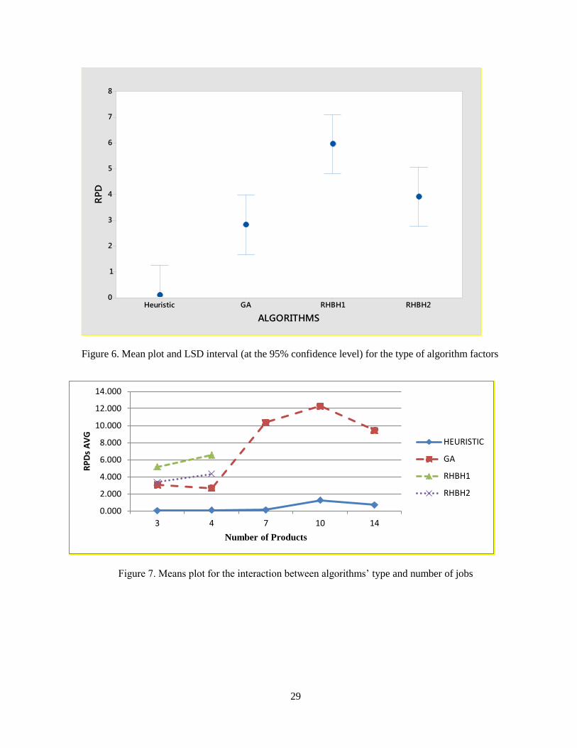
are shown in Figure 6. As can be seen, the proposed algorithm shows better statistical indices in
comparison with the others.
Please Insert Figure 6
In order to evaluate the robustness of the algorithm in different situations, possible influence of the
products number is studied. To show the mutual impact between solution procedure factors and the
number of products, the mean plot diagram is depicted (see Figure 7). It is clear that by increasing the
number of products, the difference between the performance of the proposed algorithm and the other
algorithms is increased significantly. Previous comparison also shows superiority of the proposed
algorithm compared to the three other ones.
Please Insert Figure 7
22
Figure 8 shows the run time comparison of the proposed algorithm against the others with different
problem sizes.
Please Insert Figure 8
5. Conclusions and future research directions
This paper deals with the problem of capacitated lot-sizing and scheduling in job shops with carryover
set-up and general product structure (GPS). An efficient mixed integer linear programming (MILP) model
is proposed at first to formulate the problem. Then, an available lower bound (LB) in the literature is
adapted to the problem on-hand. Due to the complexity of the studied problem, a heuristics based on the
production shifting concept is also proposed.
The numerical experiments are used to evaluate the proposed model and algorithm. The results
indicated that the model and the solution method together provide good results for use by a production
manager.
One opportunity for future research is developing heuristic and meta-heuristic algorithms for the studied
problem. Also, using the multi-objective optimization approach can be taken into consideration for further
studies.
References
[1] Guimarães, L., Klabjan, D., Almada-Lobo, B. “Modelling lotsizing and scheduling problems with
sequence dependent set-ups”, European Journal of Operational Research,239 (3), 644-662 (2014).
[2] Fandel, G., Stammen-Hegene, C. “Simultaneous lot sizing and scheduling for multi-product multi-
level production”, International Journal of Production Economic,104(2), 308–316 (2006).
[3] Meyr, H. “Simultaneous lotsizing and scheduling by combining local search with dual
reoptimization”, European Journal of Operation Research, 120(2), 311–326 (2000).
[4] Karimi, B., Fatemi-Ghomi, S.M.T., Wilson, j. “The capacitated lot sizing problem: a review of models
and algorithms”, Omega, 31, 365–378 (2003).
[5] Ouenniche, J., Bertrand, J.W.M. “The finite horizon economic lot sizing problem in job shops: the
multiple cycle approach”, International Journal of Production Economics, 74, 49-61 (2001).
[6] Ouenniche, J., Boctor, F.F., Martel, A. “The impact of sequencing decisions on multi-item lot sizing
and scheduling in flow shops”, International Journal of Production Research, 10, 2253-2270 (1999).
[7] Maravelias, C.T., Sung, C. “Integration of production planning and scheduling: Overview, challenges
and opportunities”, Computers and Chemical Engineering, 33, 1919–1930 (2009).
23
[8] Karimi-Nasab, M., Seyedhoseini, S.M. “Multi-level lot sizing and job shop scheduling with
compressible process times: A cutting plan approach”, European Journal of Operational Research, 231
(3), 598–616 (2013).
[9] Stadtler, H., Sahling, F. “A lot-sizing and scheduling model for multi-stage flow lines with zero lead
times”, European Journal of Operational Research, 225, 404–419 (2013).
[10] Babaei, M., Mohammadi, M., Fatemi-Ghomi, S.M.T. “Lot Sizing and Scheduling in Flow Shop with
Sequence-Dependent Set-ups and Backlogging”, International Journal of Computer Applications, 8,
0975–8887 (2011).
[11] Mohammadi, M., Fatemi-Ghomi, S.M.T., Karimi, B., Torabi, S.A. “MIP-based heuristics for
lotsizing in capacitated pure flow shop with sequence-dependent set-ups”, International Journal of
Production Research, 10, 2957–2973 (2010).
[12] Clark, A.R., Clark, S.J. “Rolling-horizon lot-sizing when set-up times are sequence-dependent”,
International Journal Production Research, 38(10), 2287–2308 (2000).
[13] Mohammadi, M., Fatemi-Ghomi, S.M.T., Karimi, B., Torabi, S.A. “Rolling-horizon and fix-and-
relax heuristics for the multi-product multi-level capacitated lot sizing problem with sequence-dependent
set-ups”, J. Int. Manuf, 21, 501–510 (2010).
[14] Mohammadi, M., Fatemi-Ghomi, S.M.T., Jafari, J. “A genetic algorithm for simultaneous lotsizing
and sequencing of the permutation flow shops with sequence-dependent set-ups”, International Journal of
Computer Integrated Manufacturing, 1, 87-93 (2011).
[15] Mohammadi, M., Fatemi-Ghomi, S.M.T., Karimi, B., Torabi, S.A. “MIP-based heuristics for
lotsizing in capacitated pure flow shop with sequence-dependent set-ups”, International Journal of
Production Research, 10, 2957–2973 (2010).
[16] Mohammadi, M., Jafari, N. “A new mathematical model for integrating lot sizing, loading, and
scheduling decisions in flexible flow shops”, International Journal of Advanced Manufacturing
Technology, 55, 709–721 (2011).
[17] Ramezanian, R., Saidi-Mehrabad, M., Teimoury, E. “A mathematical model for integrating lot-sizing
and scheduling problem in capacitated flow shop environments”, International Journal of Advanced
Manufacturing Technology, 347-361 (2013).
[18] Ramezanian, R., Saidi-Mehrabad, M. “Hybrid simulated annealing and MIP-based heuristics for
stochastic lot-sizing and scheduling problem in capacitated multi-stage production system”, Applied
Mathematical Modelling, 37(7), 5134–5147 (2012).
[19] Lasserre, J.B. "An Integrated Model for Job-Shop Planning and Scheduling", Management Science,
38(8), 1201-1211 (1992).
[20] Dauzere-Peres, S., Lasserre, J.B. "Integration of lot sizing and scheduling decisions in a job-shop ",
European Journal of Operational Research, 75, 413-426 (1994).
24
[21] Lalitha, J., L., Mohan, N., Pillai, V. M. "Lot streaming in [N -1] (1) + N( m ) hybrid flow shop",
Journal of Manufacturing Systems, 44, 12–21 (2017).
[22] Giglio, D., Paolucci, M., Roshani, A. "Integrated lot sizing and energy-efficient job shop scheduling
problem in manufacturing/remanufacturing systems", Journal of Cleaner Production, 148, 624- 641
(2017).
[23] Wolosewicza, C., Dauzère-Pérèsa, S., Aggouneb, R. "A Lagrangian heuristic for an integrated lot-
sizing and fixed scheduling problem", European Journal of Operational Research, 000, 1–10 (2015).
[24] Karimi-Nasab, M., Modarres, M., Seyedhoseini, S.M. "A self-adaptive PSO for joint lot
sizing and job shop scheduling with compressible process times", Applied Soft Computing, 27,
137–147 (2015).
[25] Karimi-Nasab, M., Modarres, M., Seyedhoseini, S.M. " Lot sizing and job shop scheduling with
compressible process times: A cut and branch approach", Computer and Industrial Engineering, 85, 196–
205 (2015).
[26] Urrutia,E. D. G., Aggoune, R., Dauzère-Pérès, S. "Solving the integrated lot-sizing and job-shop
scheduling problem", International Journal of Production Research, (2014), DOI:
10.1080/00207543.2014.902156.
[27] Mateus, G. R., Ravetti, M. G., de Souza, M. C., Valeriano, T.M. "Capacitated lot sizing and
sequence dependent set-up scheduling: an iterative approach for integration", Journal of Scheduling, 13,
245–259 (2010), DOI 10.1007/s10951-009-0156-2.
[28] Zhang, X.D., Yan, H.S. "Integrated optimization of production planning and scheduling for a kind of
job-shop", International Journal of Advanced Manufacturing Technology, 26, 876–886 (2005), DOI
10.1007/s00170-003-2042-y.
[29] Ouenniche, J., Boctor, F. "Sequencing. Lot sizing and scheduling of several products in job shop: the
common cycle approach", International Journal of Production Research, vol. 36, no. 4, 1125-1140
(1998).
[30] Shim, I.S., Kim, H.C., Doh, H.H., Lee, D.H. “A two-stage heuristic for single machine capacitated
lot-sizing and scheduling with sequence-dependent set-up costs”, Computers & Industrial Engineering,
61, 920–929 (2011).
[31] Afentakis, P., Gavish, P. “Optimal lot-sizing algorithms for complex product structures”, Operation
Research, 34, 237-249 (1986).
[32] Franca, P.M., Armentano, V., Berretta, R.E., Clarc, A.R. “A HEURISTIC METHOD FOR LOT-
SIZING IN MULTI-STAGE SYSTEMS”, Computers and Operations Research , 24(9), 861-874 (1997).
[33] Xie, J., Dong, J. “Heuristic Genetic Algorithms for General Capacitated Lot-Sizing Problem”,
Computer and Mathematics with Applications, 44263-276 (2001).
25
[34] Mohammadi, M., Poursabzi, O. “A rolling horizon-based heuristic to solve a multi-level general lot
sizing and scheduling problem with multiple machines (MLGLSP_MM) in job shop manufacturing
system”, Uncertain Supply Chain Management, 2, 167–178 (2014).
Biographical Notes
Omid Poursabzi a Ph.D student in industrial engineering at the Kharazmi University, Tehran,
Iran. He received his MS in Industrial Engineering from Kharazmi University, Tehran, Iran. in
2013 and BS in Industrial Engineering from Kurdistan University of Science and Technology,
Sanandaj, Iran in 2010. His research interests include production planning, econometrics and
supply chains, stochastic process and programming.
Mohammad Mohammadi is an Associate Professor in the department of industrial engineering
at the Kharazmi University, Tehran, Iran. He received his BS degree in industrial engineering
from Iran University of Science and Technology, Tehran, Iran in 2000 and his MS and PhD
degrees in industrial engineering from Amirkabir University of Technology, Tehran, Iran in 2002
and 2009 respectively. His research and teaching interests include: Applied Operations Research,
sequencing and scheduling, production planning, time series, meta-heuristics and supply chains.
Bahman Naderi is an Associate Professor of industrial engineering at the Kharazmi University
in Iran. He received his PhD in Industrial Engineering at Amirkabir University of Technology
(Iran) in the late 2009. He was also in Polytechnic University of Valencia (Spain) as a visiting
PhD student for spring semester of 2008–2009 at applied optimisation systems group. His
research and teaching interests include: production scheduling, mathematical modelling and
solution algorithms.
List of Figure Captions
Figure 1. The product structure for the example with N=3
Figure 2. A feasible solution for the example
Figure 3. The general outline of the heuristic
Figure 4. A numerical example for the encoding scheme
Figure 5. The general product structure for N=4, N=7, N=10, N=14
Figure 6. Mean plot and LSD interval (at the 95% confidence level) for the type of algorithm factors
Figure 7. Means plot for the interaction between algorithms’ type and number of jobs
Figure 8. CPU Time evaluation of the proposed heuristic against similar algorithms in the literature.
26
List of Table Captions
Table 1. The demands for the numerical example
Table 2. The results of the model and the lower bound
Table 3. Average Relative Percentage Deviation (RPD) for the algorithms grouped by N, M, T
Figure 6. The product structure for the example with N=3
Figure 7. A feasible solution for the example
27
General Procedure: Heuristic
Initializing mechanism
For j=1 to Number of Product
Product Quantity (j,:)=Output of Wagner-Within Algorithm
End
Loop
If solution is infeasible then
Smoothing mechanism
End
Improving mechanism
Merging mechanism
End
Figure 8. The general outline of the heuristic
28
Figure 9. A numerical example for the encoding scheme
1
2
4 5
3
6 7 5 86 9 7
2 3 4
10
1
7 98 10
3 4 5
12
1
62
11 13 14
1
2 3
4
Figure 10. The general product structure for N=4, N=7, N=10, N=14
29
Figure 6. Mean plot and LSD interval (at the 95% confidence level) for the type of algorithm factors
Figure 7. Means plot for the interaction between algorithms’ type and number of jobs
RHBH2RHBH1GAHeuristic
8
7
6
5
4
3
2
1
0
ALGORITHMS
RPD
0.000
2.000
4.000
6.000
8.000
10.000
12.000
14.000
3 4 7 10 14
RP
Ds
AV
G
Number of Products
HEURISTIC
GA
RHBH1
RHBH2
30
Figure 8. CPU Time evaluation of the proposed heuristic against similar algorithms in the literature.
Table 1. The demands for the numerical example
Macro
period
Product
1 2 3
1 10 30 20
2 20 20 50
Table 2. The results of the model and the lower bound
Problem size
Instance
No.
Model Lower bound
Gap Optimal
solution
Computational
time (sec)
Solution Computational
time (sec)
N=2, M=2,
T=2
1 3095 8 3059.09 <0.1 1.2%
2 4593.64 1 4519.68 <0.1 1.6%
3 1194.69 2 1158.32 <0.1 3%
4 3061.68 4 2960.31 1 3.3
5 2451.55 4 2367.66 1 3.4%
N=2, M=3, 1 2982.35 8 2700.44 1 9.4%
31
T=2 2 2227.44 12 2063.88 1 7.3%
3 3712.71 97 3668.78 2 1.2%
4 4559.12 39 4506.157 2 1.2%
5 4885.49 55 4849.19 2 0.7%
Table 3. Average Relative Percentage Deviation (RPD) for the algorithms grouped by N, M, T
Problem
Size Algorithms
N M T HEURISTIC GA RHBH1 RHBH2
3 3 3 0.060 3.322 5.028 2.091
3 3 4 0.027 2.308 4.838 3.635
3 4 3 0.002 3.580 5.678 4.358
4 3 3 0.196 0.458 4.031 1.452
4 4 4 0.180 4.289 6.251 4.386
4 4 5 0.033 4.701 9.770 5.419
4 5 4 0.012 1.166 6.149 6.051
7 5 5 0.044 9.676
7 7 5 0.198 18.880
7 7 7 0.166 2.543
10 7 7 0.008 10.290
10 10 10 1.057 25.227
10 14 10 2.699 1.295
14 10 10 0.565 8.841
14 14 14 0.836 10.011
Average 0.405 7.106 5.964 3.913
Related Documents


![[Endeavor Silver]](https://static.cupdf.com/doc/110x72/55cf8dfe550346703b8d6ced/endeavor-silver.jpg)