An improved fitting formula for the dark matter bispectrum

Prepared for submission to JCAP

An improved fitting formula for thedark matter bispectrum

Hector Gil-Marın,a,b Christian Wagner,b Frantzeska Fragkoudi,b

Raul Jimenezc,b and Licia Verdec,b

aInstitut de Ciencies de l’Espai (ICE), Facultat de Ciencies , Campus UAB (IEEC-CSIC), BellaterraE-08193, SpainbInstitut de Ciencies del Cosmos (ICC), Universitat de Barcelona (IEEC-UB), Martı i Franques 1,E-08028, SpaincICREA Institucio Catalana de Recerca i Estudis Avancats. Passeig Lluıs Companys 23, E-08010Barcelona, Spain

E-mail: [email protected], [email protected], [email protected],[email protected], [email protected]

Abstract. In this paper we present an improved fitting formula for the dark matter bispectrummotivated by the previous phenomenological approach of Ref [1]. We use a set of LCDM simulationsto calibrate the fitting parameters in the k-range of 0.03h/Mpc ≤ k ≤ 0.4h/Mpc and in the redshiftrange of 0 ≤ z ≤ 1.5. This new proposed fit describes well the BAO-features although it was notdesigned to. The deviation between the simulations output and our analytic prediction is typicallyless than 5% and in the worst case is never above 10%. We envision that this new analytic fittingformula will be very useful in providing reliable predictions for the non-linear dark matter bispectrumfor LCDM models.

arX

iv:1

111.

4477

v1 [

astr

o-ph

.CO

] 1

8 N

ov 2

011

Contents

1 Introduction 1

2 Theory 22.1 Power spectrum & bispectrum 22.2 Analytic approaches in the literature 22.3 Our analytic formula 4

3 Simulations 4

4 Results 6

5 Conclusions 9

6 Acknowledgments 9

A Appendix: bispectrum estimator & error bars 11

B Appendix: our fitting formula for non-standard LCDM models 12

C Appendix: one-loop correction terms for the power spectrum and bispectrum 13

1 Introduction

The dark matter and galaxy power spectrum have been widely used to study the growth of structure,to constrain cosmological parameters and galaxy bias models. These tools have proved very successfuland have contributed to crystallize the current LCDM model e.g., [2] and refs therein. With ongoingand forthcoming galaxy surveys, like BOSS1 and EUCLID2, the signal-to-noise of the data will increaseand the uncertainties around this model will be reduced. Higher precision data will allow the use ofnot only the two-point correlation function, but also of higher-order statistics, in order to constrainand improve our theories and models. The bispectrum (the three-point correlation function in Fourierspace) is naturally the next statistic to consider [3, 4]. Using both the power spectrum and bispectrumwe can improve our knowledge of the growth of structure and galaxy biasing [5–12], constrain possibledepartures from Gaussianity in the initial conditions of the matter density field [13–17] as well asconstrain departures from GR e.g., [18, 19].

From a theoretical point of view, perturbation theory and subsequent improvements such asrenormalized perturbation theory [20], resummed perturbation theory or time-RG flow [21] is a phys-ically well-motivated approach to study these statistical moments. Tree-level perturbation theory hasdemonstrated to describe well the behavior of the power spectrum and bispectrum at large scales.However, non-trivial computations are needed to obtain predictions at non-linear scales: the one-loopcorrection and beyond, for the power spectrum and bispectrum. For the power spectrum, how-ever, other phenomenological approaches have been demonstrated to work better for a wide range ofredshifts and different cosmologies e.g., [22–24]. For the bispectrum there are also simple phenomeno-logical models that predict its behavior at non-linear scales [1], but they fail to accurately reproducethe BAO-features [25] and are only precise at the 20%-30% level. Therefore better analytical modelsare needed to describe the bispectrum at these non-linear scales.

In this paper we improve the phenomenological description presented by [1] (hereafter SC) morethan 10 years ago. Using a set of modern simulations we fit the free parameters of our proposedanalytic formula. Thus, we obtain an improved description for the bispectrum in the LCDM model

1Baryon Oscillation Spectroscopic Survey2R. Laurejis et al, arXiv:1110.3193

– 1 –

scenario (including baryonic acoustic oscillations) in a range of 0.03h/Mpc ≤ k ≤ 0.4h/Mpc and fordifferent redshifts, 0 ≤ z ≤ 1.5.

This paper is organized as follows: in §2 we begin with a description of the density field statisticsand different analytic approaches to the dark matter bispectrum. In §3 we describe the simulations weuse to fit the parameters. In §4 we present our results, compare them with previous fitting formulaeand with 1-loop corrections and discuss the differences. We finally conclude in §5. In Appendix A,we give details of how the bispectrum and its errors are computed from simulations. In Appendix Bwe test how our formula works for other non-standard LCDM models. In Appendix C we present ashort description of 1-loop correction in Eulerian perturbation theory.

2 Theory

2.1 Power spectrum & bispectrum

The power spectrum P (k), the Fourier transform of the two-point correlation function, is one of thesimplest statistics of interest one can extract from the dark matter overdensity field δ(k),

〈δ(k)δ(k′)〉 ≡ (2π)3δD(k + k′)P (k) , (2.1)

where δD denotes the Dirac delta function and 〈. . . 〉 the ensemble average over different realizationsof the Universe. Under the assumption of an isotropic Universe, the power spectrum does not dependon the direction of the k-vector. Since we only have one observable Universe, the average 〈. . . 〉 istaken over all different directions for each k-vector. Under the hypothesis of ergodicity both averageswill yield the same result.

The second statistic of interest is the bispectrum B, defined by,

〈δ(k1)δ(k2)δ(k3)〉 ≡ (2π)3δD(k1 + k2 + k3)B(k1,k2,k3). (2.2)

The Dirac delta function ensures that the bispectrum is defined only for k-vector configurations thatform closed triangles:

∑i ki = 0. Note that δ(k1)δ(k2)δ(k3) is in general a complex number, however

once the average is taken, the imaginary part goes to zero.It is convenient to define the reduced bispectrum Q123 ≡ Q(k1,k2,k3) as,

Q123 ≡B(k1,k2,k3)

P (k1)P (k2) + P (k1)P (k3) + P (k2)P (k3)(2.3)

which takes away part of the dependence on scale and cosmology3. The reduced bispectrum is usefulwhen comparing different models, since it only has a weak dependence on cosmology and one can thusbreak degeneracies between cosmological parameters in order to isolate the effects of gravity.

The bispectrum for Gaussian initial conditions is zero and remains zero in linear theory, i.e. aslong as the k-modes evolve independently4. However, when non-linearities start to play an importantrole, mode coupling is no longer negligible and the bispectrum becomes non-zero. Thus, by measuringthe bispectrum one can extract information about how non-linear processes influence the evolution ofdark matter clustering.

2.2 Analytic approaches in the literature

In order to understand the observational data, we need accurate theoretical predictions forB(k1, k2, k3).A physically well-motivated analytic theory for doing this, is perturbation theory (PT hereafter) (see[26] for a review) or subsequent improvement such as renormalized PT, resummed PT etc.

In an Einstein de-Sitter Universe (hereafter EdS Universe) and at second order (tree-level) inEulerian perturbation theory, the bispectrum is given by [27],

B123 = 2F s2 (k1,k2)PL1 PL2 + cyc. perm., (2.4)

3For equilateral configuration and up to tree level, Q does not depend on cosmology or scale.4Wick theorem states that the n-point correlation function of a Gaussian field is always zero when n is an odd

number.

– 2 –

where B123 = B(k1,k2,k3), PLi = PL(ki) is the linear power spectrum, and the symmetrized two-point kernel F s2 is given by

F s2 (ki,kj) =5

7+

1

2cos(θij)

(kikj

+kjki

)+

2

7cos2(θij), (2.5)

where θij is the angle between the vectors ki and kj . This formula is the second order perturbationtheory contribution to the bispectrum which is the leading order contribution. On quasi-linear scales,this expression is a very good prediction but fails in the moderate non-linear regime. The dependenceon cosmology of the two-point kernel F s2 is very weak and hence the cosmology dependence of thebispectrum is almost completely contained in PLi . Because of this, in this work, we use the kernel ofEq. 2.5 even though we are dealing with the LCDM model.

One can improve the tree-level PT prediction by going one step further and including one-loopcorrections. However, at this point the computation of the bispectrum becomes cumbersome. For aninitially Gaussian δ-field this yields four additional terms to the tree-level contribution (see AppendixC for details).

An alternative way of reaching these non-linear scales, without using the one-loop correction,and to even push beyond the one-loop regime of validity, is with phenomenologically motivated mod-els. Phenomenological formulae can give simpler expressions in the non-linear regime and accuratepredictions for the bispectrum. However, their physical motivation is limited and they usually havefree parameters that need to be calibrated using N-body simulations.

SC proposed a fitting formula based on the structure of the formula of Eq. 2.4. It consistsin replacing the linear power spectrum by the non-linear one in Eq. 2.4 and the EdS two-pointsymmetrized kernel by

F eff2 (ki,kj) =

5

7a(ni, ki)a(nj , kj) (2.6)

+1

2cos(θij)

(kikj

+kjki

)b(ni, ki)b(nj , kj) +

2

7cos2(θij)c(ni, ki)c(nj , kj),

where the functions a(n, k), b(n, k) and c(n, k) are chosen to interpolate between the tree-level resultsand the hyper-extended perturbation theory regime (HEPT) [28],

a(n, k) =1 + σa68 (z)[0.7Q3(n)]1/2(qa1)n+a2

1 + (qa1)n+a2,

b(n, k) =1 + 0.2a3(n+ 3)qn+3

1 + qn+3.5, (2.7)

c(n, k) =1 + 4.5a4/[1.5 + (n+ 3)4](qa5)n+3

1 + (qa5)n+3.5.

Here n is the slope of the linear power spectrum at k,

n ≡ d logPL(k)

d log k(2.8)

and q ≡ k/knl, where knl is the scale where non-linearities start to be important and is defined as,

k3nlP

L(knl)

2π2≡ 1; (2.9)

ai are free parameters that must be fitted using data from simulations. In particular, SC propose thevalues,

a1 = 0.25, a2 = 3.5, a3 = 2, a4 = 1, a5 = 2, a6 = −0.2 .

The function Q3(n) is given by

Q3(n) =4− 2n

1 + 2n+1. (2.10)

– 3 –

With all these changes, the SC approach reads,

B123 = 2F eff2 (k1,k2)P1P2 + cyc. perm., (2.11)

where Pi is the non-linear power spectrum at ki. On large scales, where the functions a, b and c→ 1 we recover the tree-level PT formula for the bispectrum. On the other hand, on small scalesa2 → (7/10)Q3 and b and c → 0 and we obtain Q123 → Q3(n), which is the prediction of HEPT.

Another approach based on phenomenological formulae, is the one presented by [25]. The mainidea is to rescale the linear formula of the bispectrum, by using some scale transformation in k.This way, the tree-level formula can easily be extended up to non-linear scales using the ansatz

ki =[1 + ∆2

NL(ki)]−1/3

ki; where ∆2NL(k) = P (k)k3/(2π2).

This approach has by definition the drawback that it does not preserve the BAO-features of thebispectrum. In particular, the rescaling of k produces a spurious rescaling of the peaks and troughs ofthe BAO wiggles that do not match with the data, producing higher deviations than the SC approach.Because of that, we do not consider this approach in this paper.

2.3 Our analytic formula

Our approach in this paper is inspired by the SC approach. It consists of not only refitting the aiparameters from Eq. 2.7 but of also modifying their expression to make it more suitable for currentprecision N-body data and consider the redshift range of 0 ≤ z ≤ 1.5. In order to do that, we usesimulations with more particles, larger box sizes, and more realizations (and thus higher precision,better statistics and better error-control) with respect to previous works; we also consider snapshotsat different redshifts. In order to improve the fitting precision, we also add 3 more parameters to theoriginal model. The modified functions a(n, k), b(n, k), c(n, k) then read,

a(n, k) =1 + σa68 (z)[0.7Q3(n)]1/2(qa1)n+a2

1 + (qa1)n+a2,

b(n, k) =1 + 0.2a3(n+ 3)(qa7)n+3+a8

1 + (qa7)n+3.5+a8, (2.12)

c(n, k) =1 + 4.5a4/[1.5 + (n+ 3)4](qa5)n+3+a9

1 + (qa5)n+3.5+a9.

Note that one recovers the original SC formulae in the limit of a7 → 1 and a8, a9 → 0.The original SC formula was not designed to reproduce the BAO features. Applying this formula

to a power spectrum with BAOs produces unphysical oscillations. These oscillations are much largerthan those observed in simulations (see black dashed line in the right panel of Fig. 1). Theseoscillations are caused by the oscillatory behavior of the slope parameter n. To avoid this problemour approach is to smooth the oscillatory behavior of the parameter n by means of splines, as is shownin the blue solid line of the left panel of Fig. 1. This provides an improved fit to the BAO-features, asit is shown by the blue solid line in the right panel of Fig. 1. In order to smooth out n we calculateits spline by taking a number of points n(k), where the points are chosen to be in the middle of theamplitude of each wiggle, such that when the points are connected a smooth line would pass throughthem. These points are used in the spline routine, and their second order derivatives are calculatedfor each point k. This output is then fed into the spline routine, which returns a smoothed value ofn for each value of k.

Our method consists in using this smoothed n and refit all the free ai parameters from Eq.2.12 using the reduced bispectrum data from N-body simulations. In particular, we use the followingtriangle configurations at different redshifts: θ12/π = 0.1, 0.2, . . . , 0.9, k2/k1 = 1.0, 1.5, 2.0, 2.5 andz = 0, 0.5, 1, 1.5.

3 Simulations

The simulations in this paper consist of two different sets, namely A and B. Each simulation ischaracterized by the box size, Lb, the number of particles, Np, and the number of independent runs,

– 4 –

-3-2.5

-2-1.5

-1-0.5

0 0.5

0.01 0.1 0.5

n(k)

k [h/Mpc]

0.6

0.8

1.0

1.2

1.4

0.03 0.1 0.2

Q(k

1)

k1 [h/Mpc]

Figure 1. Left panel: The slope n(k) (Eq. 2.8) from the linear power spectrum without smoothing (blackdashed line) and with a spline smoothing (blue solid line). Right panel: Q(k1) for k2/k1 = 2 and θ12 = 0.6π.Red circles are data from simulations A and red squares from simulations B (see Table 1 for details on thesimulations). Black dashed line is SC prediction without any spline in n(k) and blue solid line with the splinein n(k).

A BLb [Mpc/h] 2400 1875

Np 7683 10243

Nr 40 3kN/2 [h/Mpc] 0.25 0.43

softening [kpc/h] 90 40

Table 1. Simulations details for simulations A and B. Lb is the box size, Np is the number of particles, Nr

is the number of independent realizations and kN/2 is the half Nyquist frequency.

Nr. Details about the two simulations are given in Table 1. As a rule of thumb, a maximum threshold

in k for trusting the data is set by half the Nyquist frequency, defined as kN/2 = πN1/3p /(4Lb). For

all the plots and results shown in this paper the Nyquist frequency is never exceeded.Both A and B simulations consist in a flat LCDM cosmology with cosmological parameters

consistent with observational data. The cosmology used is ΩΛ = 0.73, Ωm = 0.27 h = 0.7, Ωbh2 =

0.023, ns = 0.95 and σ8(z = 0) = 0.7913. The initial conditions were generated at z = 19 andz = 49 for simulations A and B respectively, by displacing the particles according to the second-orderLagrangian PT from their initial grid points. The initial power spectrum of the density fluctuationswas computed by CAMB [29]. Taking only the gravitational interaction into account, the simulationwas performed with GADGET-2 code [30].

As we estimate the error of the bispectrum from its dispersion among different realizations (seeEq. A.5 in Appendix A for details), and given that we only have 3 simulations of type B, we divideeach of these 3 boxes into 8 sub-boxes. Each of these 24 sub-boxes is then treated as if it werean independent realization with smaller box size, L′b = 937.5h/Mpc, where each of these sub-boxescontains about 5123 particles. The measurements of the bispectrum from sub-boxes suffer from twoissues: a) the measurements are not completely independent and more importantly b) the sub-boxesare affected by modes larger than sub-box size. As a consequence of this, a new source of non-Gaussianerrors arises for the power spectrum and bispectrum estimation, called beat-coupling effect [31–33].However, by using the mean density measured in each sub-box instead of the global mean densityfor the normalization of the density contrast, δ ≡ ρ/ρ − 1, this effect gets strongly suppressed [34].Hence, we expect that on overlapping scales the bispectrum errors estimated from simulation B to beslightly larger than those from A. This is shown in Appendix A.

In order to obtain the dark matter field from particles we discretize each box of simulation A

– 5 –

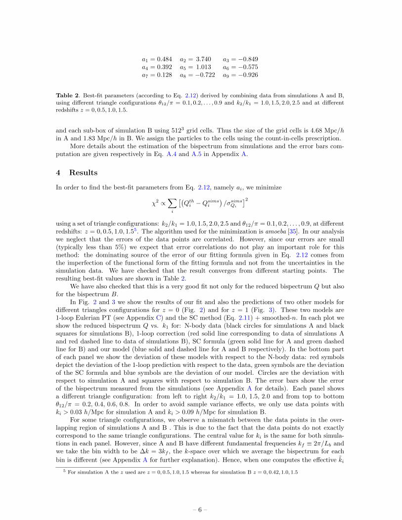
a1 = 0.484 a2 = 3.740 a3 = −0.849a4 = 0.392 a5 = 1.013 a6 = −0.575a7 = 0.128 a8 = −0.722 a9 = −0.926

Table 2. Best-fit parameters (according to Eq. 2.12) derived by combining data from simulations A and B,using different triangle configurations θ12/π = 0.1, 0.2, . . . , 0.9 and k2/k1 = 1.0, 1.5, 2.0, 2.5 and at differentredshifts z = 0, 0.5, 1.0, 1.5.

and each sub-box of simulation B using 5123 grid cells. Thus the size of the grid cells is 4.68 Mpc/hin A and 1.83 Mpc/h in B. We assign the particles to the cells using the count-in-cells prescription.

More details about the estimation of the bispectrum from simulations and the error bars com-putation are given respectively in Eq. A.4 and A.5 in Appendix A.

4 Results

In order to find the best-fit parameters from Eq. 2.12, namely ai, we minimize

χ2 ∝∑i

[(Qthi −Qsimsi

)/σsimsQi

]2using a set of triangle configurations: k2/k1 = 1.0, 1.5, 2.0, 2.5 and θ12/π = 0.1, 0.2, . . . , 0.9, at differentredshifts: z = 0, 0.5, 1.0, 1.55. The algorithm used for the minimization is amoeba [35]. In our analysiswe neglect that the errors of the data points are correlated. However, since our errors are small(typically less than 5%) we expect that error correlations do not play an important role for thismethod: the dominating source of the error of our fitting formula given in Eq. 2.12 comes fromthe imperfection of the functional form of the fitting formula and not from the uncertainties in thesimulation data. We have checked that the result converges from different starting points. Theresulting best-fit values are shown in Table 2.

We have also checked that this is a very good fit not only for the reduced bispectrum Q but alsofor the bispectrum B.

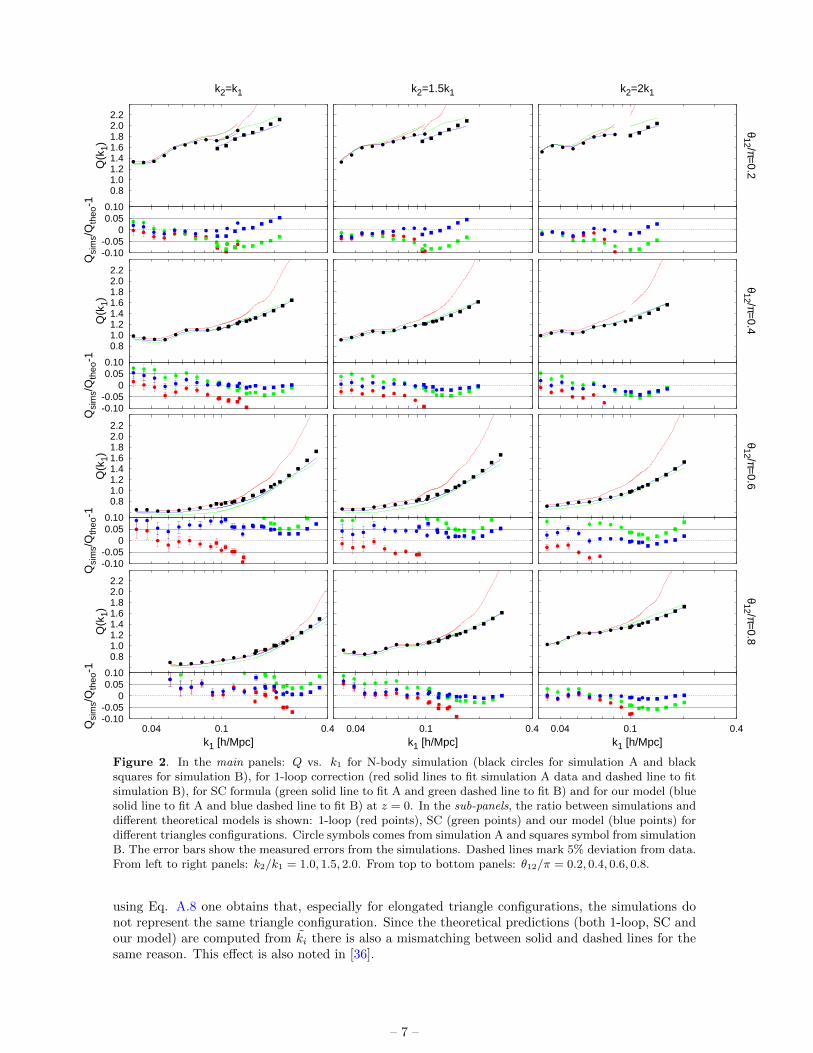
In Fig. 2 and 3 we show the results of our fit and also the predictions of two other models fordifferent triangles configurations for z = 0 (Fig. 2) and for z = 1 (Fig. 3). These two models are1-loop Eulerian PT (see Appendix C) and the SC method (Eq. 2.11) + smoothed-n. In each plot weshow the reduced bispectrum Q vs. k1 for: N-body data (black circles for simulations A and blacksquares for simulations B), 1-loop correction (red solid line corresponding to data of simulations Aand red dashed line to data of simulations B), SC formula (green solid line for A and green dashedline for B) and our model (blue solid and dashed line for A and B respectively). In the bottom partof each panel we show the deviation of these models with respect to the N-body data: red symbolsdepict the deviation of the 1-loop prediction with respect to the data, green symbols are the deviationof the SC formula and blue symbols are the deviation of our model. Circles are the deviation withrespect to simulation A and squares with respect to simulation B. The error bars show the errorof the bispectrum measured from the simulations (see Appendix A for details). Each panel showsa different triangle configuration: from left to right k2/k1 = 1.0, 1.5, 2.0 and from top to bottomθ12/π = 0.2, 0.4, 0.6, 0.8. In order to avoid sample variance effects, we only use data points withki > 0.03 h/Mpc for simulation A and ki > 0.09 h/Mpc for simulation B.

For some triangle configurations, we observe a mismatch between the data points in the over-lapping region of simulations A and B . This is due to the fact that the data points do not exactlycorrespond to the same triangle configurations. The central value for ki is the same for both simula-tions in each panel. However, since A and B have different fundamental frequencies kf ≡ 2π/Lb andwe take the bin width to be ∆k = 3kf , the k-space over which we average the bispectrum for each

bin is different (see Appendix A for further explanation). Hence, when one computes the effective ki

5 For simulation A the z used are z = 0, 0.5, 1.0, 1.5 whereas for simulation B z = 0, 0.42, 1.0, 1.5

– 6 –

-0.10-0.05

00.050.10

Qsi

ms/

Qth

eo-1

0.81.01.21.41.61.82.02.2

Q(k

1)k2=k1

k2=1.5k1

θ12 /π=

0.2

k2=2k1

-0.10-0.05

00.050.10

Qsi

ms/

Qth

eo-1

0.81.01.21.41.61.82.02.2

Q(k

1)

θ12 /π=

0.4

-0.10-0.05

00.050.10

Qsi

ms/

Qth

eo-1

0.81.01.21.41.61.82.02.2

Q(k

1)

θ12 /π=

0.6

-0.10-0.05

00.050.10

0.04 0.1 0.4Qsi

ms/

Qth

eo-1

k1 [h/Mpc]

0.81.01.21.41.61.82.02.2

Q(k

1)

0.04 0.1 0.4k1 [h/Mpc]

0.04 0.1 0.4k1 [h/Mpc]

θ12 /π=

0.8

Figure 2. In the main panels: Q vs. k1 for N-body simulation (black circles for simulation A and blacksquares for simulation B), for 1-loop correction (red solid lines to fit simulation A data and dashed line to fitsimulation B), for SC formula (green solid line to fit A and green dashed line to fit B) and for our model (bluesolid line to fit A and blue dashed line to fit B) at z = 0. In the sub-panels, the ratio between simulations anddifferent theoretical models is shown: 1-loop (red points), SC (green points) and our model (blue points) fordifferent triangles configurations. Circle symbols comes from simulation A and squares symbol from simulationB. The error bars show the measured errors from the simulations. Dashed lines mark 5% deviation from data.From left to right panels: k2/k1 = 1.0, 1.5, 2.0. From top to bottom panels: θ12/π = 0.2, 0.4, 0.6, 0.8.

using Eq. A.8 one obtains that, especially for elongated triangle configurations, the simulations donot represent the same triangle configuration. Since the theoretical predictions (both 1-loop, SC andour model) are computed from ki there is also a mismatching between solid and dashed lines for thesame reason. This effect is also noted in [36].

– 7 –

-0.10-0.05

00.050.10

Qsi

ms/

Qth

eo-1

0.81.01.21.41.61.82.02.2

Q(k

1)k2=k1

k2=1.5k1

θ12 /π=

0.2

k2=2k1

-0.10-0.05

00.050.10

Qsi

ms/

Qth

eo-1

0.81.01.21.41.61.82.02.2

Q(k

1)

θ12 /π=

0.4

-0.10-0.05

00.050.10

Qsi

ms/

Qth

eo-1

0.81.01.21.41.61.82.02.2

Q(k

1)

θ12 /π=

0.6

-0.10-0.05

00.050.10

0.04 0.1 0.4Qsi

ms/

Qth

eo-1

k1 [h/Mpc]

0.81.01.21.41.61.82.02.2

Q(k

1)

0.04 0.1 0.4k1 [h/Mpc]

0.04 0.1 0.4k1 [h/Mpc]

θ12 /π=

0.8

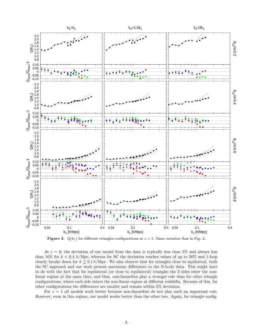
Figure 3. Q(k1) for different triangles configurations at z = 1. Same notation that in Fig. 2.

At z = 0, the deviation of our model from the data is typically less than 5% and always lessthan 10% for k < 0.4 h/Mpc, whereas for SC the deviation reaches values of up to 20% and 1-loopclearly breaks down for k & 0.1h/Mpc. We also observe that for triangles close to equilateral, boththe SC approach and our work present maximum differences to the N-body data. This might haveto do with the fact that for equilateral (or close to equilateral) triangles the 3 sides enter the non-linear regime at the same time, and thus, non-linearities play a stronger role than for other triangleconfigurations, where each side enters the non-linear regime at different redshifts. Because of this, forother configurations the differences are smaller and remain within 5% deviation.

For z = 1 all models work better because non-linearities do not play such an important role.However, even in this regime, our model works better than the other two. Again, for triangle config-

– 8 –

urations close to equilateral, our model reaches its maximum deviation of about 10%. At z = 1, allother triangle configurations typically have errors within 5%.

As a cross-check, in Appendix B we compare our model with another set of simulations of non-standard LCDM model. In particular for equilateral configurations, our formula reaches deviationsup to 10%. However for the scalene configurations k2 = 2k1 the deviations are only of order 3%. Inthe cases studied here our model improves significantly the SC fitting formula.

5 Conclusions

In this paper we propose a new simple formula to compute the dark matter bispectrum in the mod-erate non-linear regime (k < 0.4h/Mpc) and for redshifts z ≤ 1.5. Our method is inspired by theapproach presented in [1], but includes a modification of the original formulae, namely Eq. 2.12, anda prescription to better describe the BAO oscillations.

Using LCDM simulations we fit the free parameters of our model. We end up with a simpleanalytic formula that is able to predict accurately the bispectrum for a LCDM Universe includingthe effects of BAO. Our main results are summarized by Eq. 2.11 where the kernel is given by Eq.2.6, the functions a, b, c are now given by a, b, c of Eq. 2.12, the fitting coefficients take the valuesreported in Table 2 and the function Q3(n) is still given by Eq. 2.10. The local slope of the linearpower spectrum n(k) is not any more given directly by Eq. 2.8 but is a smoothed (BAO-free, butwith the same broadband behavior) function of k.

The main conclusions of our work are listed below.

1. Our method is able to predict the dark matter bispectrum for a wide range of triangle con-figurations up to k = 0.4h/Mpc and for a redshift range 0 ≤ z ≤ 1.5. In particular, for thereduced bispectrum, our fitting formula agrees within 5% with N-body data for most of thetriangle configurations and always within 10% for the worst cases. This presents a considerableimprovement over previous phenomenological approaches and over the prediction of Eulerianperturbation theory.

2. The equilateral and quasi-equilateral configurations are the ones for which our model deviatesmost strongly from N-body data. We interpret this as being due to the fact that when the 3sides of the triangle are similar, non-linearities start to play a role at the same time, and thus,the effect on the bispectrum is stronger than when the non-linearities enter at different times, i.e.for elongated triangles. Other methods, like the one described by SC show the same behavior.

3. We have checked that our model also works well for non-standard LCDM cosmologies (seeAppendix B). In particular, we have checked that for k2 = 2k1 the deviation between N-bodydata and our model is never higher than 3% and for equilateral triangles reaches 10%. Alsoin these non-standard LCDM cases studied here, our model works better than the SC fittingformula.

We envision that this new analytic fitting formula will be very useful in providing a reliableprediction for the non-linear dark matter bispectrum for LCDM models. In particular, simple analyticpredictions with high accuracy will be needed for the data analysis in the forthcoming era of precisiondata.

6 Acknowledgments

We thank Fabian Schmidt for providing the non-standard LCDM simulations used in Appendix B.Hector Gil-Marın thanks the Argerlander Institut fur Astronomie at the University of Bonn for hos-pitality. Hector Gil-Marın is supported by CSIC-JAE grant. Christian Wagner and Licia Verdeacknowledge support of FP7-IDEAS-Phys.LSS 240117.

– 9 –

References

[1] Scoccimarro, R., & Couchman, H. M. P. 2001, MNRAS, 325, 1312

[2] Reid, B. A., Percival, W. J., Eisenstein, D. J., et al. 2010, MNRAS, 404, 60

[3] Fry, J. N., & Melott, A. L. 1985, ApJ, 292, 395

[4] Kayo, I., Suto, Y., Nichol, R. C., et al. 2004, PASJ, 56, 415

[5] Guo, H., & Jing, Y. P. 2009, ApJ, 702, 425

[6] Fry, J. N. 1994, Physical Review Letters, 73, 215

[7] Verde, L., Heavens, A. F., Matarrese, S., & Moscardini, L. 1998, MNRAS, 300, 747

[8] Matarrese, S., Verde, L., & Heavens, A. F. 1997, MNRAS, 290, 651

[9] Fry, J. N., Melott, A. L., & Shandarin, S. F. 1995, MNRAS, 274, 745

[10] Scoccimarro, R., Feldman, H. A., Fry, J. N., & Frieman, J. A. 2001, ApJ, 546, 652

[11] Feldman, H. A., Frieman, J. A., Fry, J. N., & Scoccimarro, R. 2001, Physical Review Letters, 86, 1434

[12] Verde, L., Heavens, A. F., Percival, W. J., et al. 2002, MNRAS, 335, 432

[13] Jeong, D., & Komatsu, E. 2009, ApJ, 703, 1230

[14] Verde, L., Wang, L., Heavens, A. F., & Kamionkowski, M. 2000, MNRAS, 313, 141

[15] Verde, L., Jimenez, R., Kamionkowski, M., & Matarrese, S. 2001, MNRAS, 325, 412

[16] Sefusatti, E., & Komatsu, E. 2007, Phys. Rev. D, 76, 083004

[17] Scoccimarro, R., Sefusatti, E., & Zaldarriaga, M. 2004, Phys. Rev. D, 69, 103513

[18] Gil-Marın, H., Schmidt, F., Hu, W., Jimenez, R., & Verde, L. 2011, J. Cosmology Astropart. Phys., 11,19

[19] Shirata, A., Suto, Y., Hikage, C., Shiromizu, T., & Yoshida, N. 2007, Phys. Rev. D, 76, 044026

[20] Crocce, M., Scoccimarro , R., 2006, Phys.Rev.D, 73:063519

[21] Pietroni, M. 2008, J. Cosmology Astropart. Phys., 10, 36

[22] Cooray, A., & Sheth, R. 2002, Phys. Rep., 372, 1

[23] Ma, C.-P., & Fry, J. N. 2000, ApJ, 543, 503

[24] Smith, R. E., Peacock, J. A., Jenkins, A., et al. 2003, MNRAS, 341, 1311

[25] Pan, J., Coles, P., & Szapudi, I. 2007, MNRAS, 382, 1460

[26] Bernardeau, F., Colombi, S., Gaztanaga, E., & Scoccimarro, R. 2002, Phys. Rep., 367, 1

[27] Fry, J. N. 1984, ApJ, 279, 499

[28] Scoccimarro, R., & Frieman, J. A. 1999, ApJ, 520, 35

[29] Lewis, A., Challinor, A., & Lasenby, A. 2000, ApJ, 538, 473

[30] Springel, V. 2005, MNRAS, 364, 1105

[31] Hamilton, A. J. S., Rimes, C. D., & Scoccimarro, R. 2006, MNRAS, 371, 1188

[32] Rimes, C. D., & Hamilton, A. J. S. 2006, MNRAS, 371, 1205

[33] Sefusatti, E., Crocce, M., Pueblas, S., & Scoccimarro, R. 2006, Phys. Rev. D, 74, 023522

[34] De Putter, R., et al. in preparation

[35] Press, W. H., Teukolsky, S. A., Vetterling, W. T., & Flannery, B. P. 1992, Cambridge: UniversityPress, —c1992, 2nd ed.,

[36] Sefusatti, E., Crocce, M., & Desjacques, V. 2010, MNRAS, 406, 1014

[37] Scoccimarro, R., Colombi, S., Fry, J. N., Frieman, J. A., Hivon, E., & Melott, A. 1998, ApJ, 496, 586

– 10 –

[38] Guo, H., & Jing, Y. P. 2009, ApJ, 698, 479

A Appendix: bispectrum estimator & error bars

Here we present details on the computation of the bispectrum and its error bars from N-body simula-tions. Moreover, we compare our error estimates with the Gaussian analytic predictions and discussthe differences.

We start by defining the estimator for the bispectrum as,

B(k1,k2,k3) ≡ VfVB

∫k1

d3q1

∫k2

d3q2

∫k3

d3δD(q1 + q2 + q3)δq1δq2δq3 (A.1)

where Vf = (2π)3/L3b ≡ k3

f is the volume of the fundamental cell, kf . The integration is definedover the bin ki − ∆ki/2 < qi < ki + ∆ki/2. In this paper we always take ∆k = 3kf . VB is thesix-dimensional volume of triangles defined by the triangle sizes k1, k2 and k3 with uncertainty ∆k.Its value can be approximated by

VB(k1, k2, k3) =

∫k1

d3q1

∫k2

d3q2

∫k3

d3q3 δD(q1 + q2 + q3) ' 8π2k1k2k3∆k3 (A.2)

which is good enough for not too small values of ki. The variance associated to this estimator dependson higher-order correlation functions: up to the 6-point connected correlation function. However, themain contribution to the variance is given by the power spectrum. Assuming that the fields areGaussian, the variance associated to estimator presented above is [37],

∆B2(k1,k2,k3) = sBVfVB

(2π)3P (k1)P (k2)P (k3) (A.3)

where the symmetry factor is sB = 6, 2, 1 for equilateral, isosceles or scalene configurations. Thefactor (2π)3 comes from our definition of the power spectrum and bispectrum in Eq. 2.1 and 2.2.

On the other hand, the discretized version of this estimator used in this paper is, B

B(k1,k2,k3) =L6b

Ntri

Ntri∑j

Re[δdj (k1)δdj (k2)δdj (k3)

](A.4)

where Ntri is the number of random triangle configurations used to compute the bispectrum; andj runs over these triangle configurations. For this work we use a number of random triangles thatincreases with k in the same way as the number of fundamental triangles: ∼ VB/V

2f . It reaches up

to Ntri ∼ 109 for scales k ∼ 0.4h/Mpc. We have checked that increasing the number of randomtriangles beyond this value has no effect neither in the value of the bispectrum nor in its error.The index d in the δ field stands for a discrete and dimensionless quantity. Therefore the quantityRe[δdj (k1)δdj (k2)δdj (k3)

]needs to be rescaled with the factor L6

b to make B matching with the definition

of the bispectrum in Eq. 2.2. We compute the variance of this estimator B by the sample variancederived from the Nr realizations,

∆B2(k1,k2,k3) =

1

Nr − 1

Nr∑i

(Bi(k1,k2,k3)− 〈B(k1,k2,k3)〉

)2

(A.5)

where Bi is the bispectrum derived from the realization i and 〈B〉 is the mean over all realizations,

〈B(k1,k2,k3)〉 ≡ 1

Nr

Nr∑i

Bi(k1,k2,k3) . (A.6)

– 11 –

104

105

106

107

108

109

0.03 0.1 0.4

∆B [(

Mpc

/h)6 ]

k1 [h/Mpc]

0.5

1.0

5.0

0.03 0.1 0.4

∆Bsi

ms /∆

Bth

eo

k1 [h/Mpc]

Figure 4. Left panel: ∆B for k2/k1 = 1 and θ12 = 0.6π triangles as a function of k1 derived from simulationsA (red squares) and from simulations B (green circles). Blue line is the theoretical prediction according toEq. A.3. Right panel: ∆B/∆B for simulations A (red squares) and B (green circles)

The error on the mean 〈B〉 is then simply given by

σ〈B〉 = ∆B/√Nr . (A.7)

When comparing the measured N-body bispectrum with theoretical models and also when com-paring Eq. A.3 with Eq. A.5, it is important to take into account the effect on the finite size of thetriangle bins: each configuration is defined in terms of the sides of the triangle ki ± ∆k/2. In thiscase, we are assuming ∆k = 3kf and a large number of fundamental triangles fit into this bin. Forcertain configurations, it turns out that we have more triangles with k larger than the central value,ki. Because of that, one must correct the sides of the triangles by

ki =1

Ntri

Ntri∑j

kji (A.8)

where i = 1, 2, 3 for each dimension and the sum is taken over all random triangle generated in thebin. This correction is extremely important at large scales and for very squeezed triangles, and lessimportant for equilateral configuration.

In Fig 4 we present a comparison of the error estimation from theoretical models (Eq. A.3) andsimulations (Eq. A.5). In the left panel we show the error of the bispectrum associated to a volume of1 single box for ∆k = 3kf : using the theoretical model and the simulations for the case of k2/k1 = 1and θ12 = 0.6π triangle configurations. The blue line shows the theoretical model prediction for theerror of the bispectrum of one single realization using the non-linear power spectra from simulationsA and B (Eq. A.3); whereas the red squares and green circles show the dispersion among the runs ofsimulations A and B respectively (Eq. A.5). In the right panel the ratio between the errors accordingto the simulations and the Gaussian prediction is plotted for simulations A (red squares) and B (greencircles). The error estimates of simulations A agrees well with the theoretical model. On the otherhand, on small scales the error estimates of simulations B is larger than the theoretical model andfurther increase with decreasing scale. Similar results were found by [38]. These differences are dueto the fact that Eq. A.3 neglects any higher-order contributions (because it assumes Gaussianity).However, at small scales this is no longer a good approximation as it is shown in [33]. Furthermore,the errors of simulations B have been estimated by dividing each of the 3 simulation boxes into 8sub-boxes. This introduces extra non-Gaussian terms [33] that are not taken into account in Eq. A.3.

B Appendix: our fitting formula for non-standard LCDM models

Here we test how our model works with different LCDM simulations to those we have used to fitthe ai parameters. In particular, we test our model with LCDM simulations with a f(R)-like powerspectrum. For a full description of the simulations and the f(R) gravity we refer the reader to [18].

– 12 –

These simulations were run with ENZO code and have slightly different cosmology than the onesused in the rest of this paper: ΩΛ = 0.76, Ωm = 0.24, Ωb = 0.04181, h = 0.73. They consist of 6realizations that contain 2563 particles in a box of 400 Mpc/h per side. Their half Nyquist frequencyis kN/2 = 0.5 h/Mpc.

In Fig. 5 the reduced bispectrum Q is shown: in the right panel as a function of the anglebetween k1 and k2, namely θ12, for k2 = 2k1; in the left panel as a function of k1 for equilateralconfiguration, both for z = 0. All panels correspond to a LCDM model with no BAOs whose initialconditions make their power spectrum look like a f(R)-like one. In order to do that a running indexhas been adopted in the initial conditions (see Table 1 in [18] for details). Panels correspond to LCDMsimulations that match with f(R) models whose |fR0| parameter6 is: 10−4 (top panels), 10−5 (middlepanels) and 10−6 (bottom panels ).

Black points are data from simulations, green line is the SC prediction and blue line the predictionof our model. In the right panel we only compare data points for 0.4 < θ12/π < 0.9 and in the leftpanel 0.1h/Mpc < k < 0.5h/Mpc in order to ensure that all the ki are smaller than half Nyquistfrequency.

Considering the right panels of Fig. 5 (k2 = 2k1 = 0.4h/Mpc), we see that our model describesthe data within about 3%. In particular for small scales (θ12 < 0.7π), both SC and our model agreewith the simulations data well; however at large scales (θ12 > 0.7π), our model fits the data pointsbetter. In the left panel of Fig. 5 (equilateral configuration), we see that our model shows deviationsup to 10%. As for the standard LCDM model, the equilateral configuration is the one with the largestdeviations. However even in this case, our formula behaves better than the SC model, especially atsmall scales.

Therefore we conclude that our formula is general enough to be applied also to some non-standardLCDM models and in particular works better than SC at small scales.

C Appendix: one-loop correction terms for the power spectrum and bis-pectrum

Here we present a short description of the equations used to compute the one-loop correction inEulerian perturbation theory for the bispectrum shown in Fig. 2 and 3. For a detailed description ofPT see [26].

Up to one-loop, the power spectrum can be expressed as,

P (k) = P (0)(k) + P (1)(k) + . . . (C.1)

where P (0)(k) = PL(k) is the linear term and P (1)(k) = P13(k) + P22(k) is the one loop correction.For Gaussian initial conditions, the one-loop term consist of two terms7,

P22 =2

(2π)3

∫d3qF s2

2(q,k− q)PL(q)PL(|k− q|) (C.2)

P13 =6

(2π)3PL(k)

∫d3qF s3 (k,q,−q)PL(q) (C.3)

P22 accounts for the mode coupling between waves with wave-vectors k − q and q, whereas P13 canbe interpreted as the one-loop correction to the linear propagator.

Similarly to the power spectrum, the bispectrum up to one loop consists of two terms,

B(k1,k2,k3) = B(0)(k1,k2,k3) +B(1)(k1,k2,k3) + . . . (C.4)

For Gaussian initial conditions, the first non-zero term is the second-order contribution B(0) which istree level correction, whereas B(1) is the one-loop correction. The tree level term can be expressed as,

B(0)(k1,k2,k3) = 2F s2 (k1,k2)PL(k1)PL(k2) + 2 cyc. perm. (C.5)

6see Eq. 2.3 in [18] for a definition of fR07The (2π)3 in the denominator comes from the definition of the power spectrum and bispectrum in Eq. 2.1 and 2.2

– 13 –

-0.10-0.05

00.050.10

Qsi

ms/

Qth

eo-1

0.81.01.21.41.61.82.0

Q(k

1)

equilateral

-0.05-0.025

00.0250.05

Qsi

ms/

Qth

eo-1

1.41.51.61.71.81.92.0

Q(θ

12)

|fR0 |=

10-4

k2=2k1=0.4 h/Mpc

-0.10-0.05

00.050.10

Qsi

ms/

Qth

eo-1

0.81.01.21.41.61.82.0

Q(k

1)

-0.05-0.025

00.0250.05

Qsi

ms/

Qth

eo-1

1.41.51.61.71.81.92.0

Q(θ

12)

|fR0 |=

10-5

-0.10-0.05

00.050.10

0.1 0.2 0.3 0.4 0.5Qsi

ms/

Qth

eo-1

k1 [h/Mpc]

0.81.01.21.41.61.82.0

Q(k

1)

-0.05-0.025

00.0250.05

0.4 0.5 0.6 0.7 0.8 0.9Qsi

ms/

Qth

eo-1

θ12/π

1.41.51.61.71.81.92.0

Q(θ

12)

|fR0 |=

10-6

Figure 5. In the left panels: Q vs. k1 for equilateral configuration. In the right panels Q vs θ12/π fork2 = 2k1 = 0.4h/Mpc. From top to bottom we show different non-standard LCDM models. All the panelscorrespond to LCDM models with f(R)-like power spectrum from [18]. Top panels correspond to matchingto |fR0| = 10−4; middle panels to |fR0| = 10−5; bottom panels to |fR0| = 10−6. The sub-panel shows thecorresponding ratio between simulations and different theoretical models: SC (green points) and our work(blue points). In the right sub-panels, dashed lines mark 2.5% deviation, whereas in the left panels mark the5% deviation. The bispectrum and its error are estimated by Eq. A.6 and A.7 (see Appendix A).

whereas the one loop consist of four terms (only for Gaussian initial conditions),

B(1)(k1,k2,k3) = BI222(k1,k2,k3) +B123(k1,k2,k3) + (C.6)

+ BII123(k1,k2,k3) +BI114(k1,k2,k3)

– 14 –

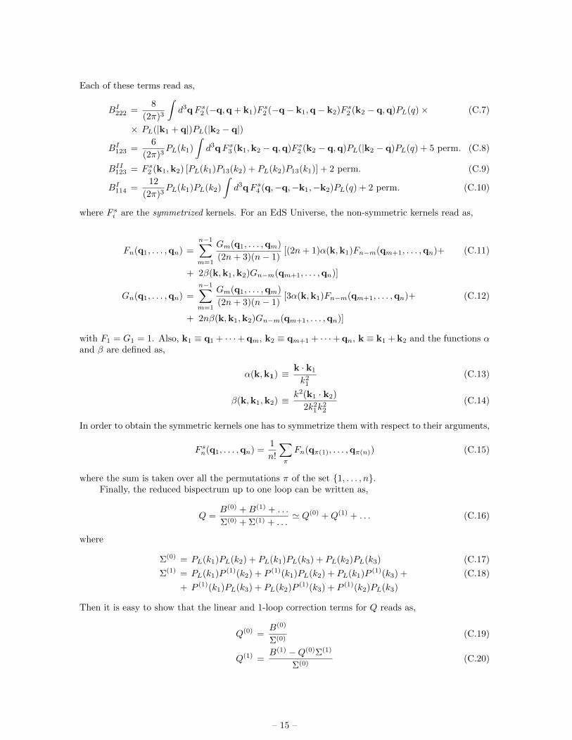
Each of these terms read as,

BI222 =8

(2π)3

∫d3qF s2 (−q,q + k1)F s2 (−q− k1,q− k2)F s2 (k2 − q,q)PL(q)× (C.7)

× PL(|k1 + q|)PL(|k2 − q|)

BI123 =6

(2π)3PL(k1)

∫d3qF s3 (k1,k2 − q,q)F s2 (k2 − q,q)PL(|k2 − q)PL(q) + 5 perm. (C.8)

BII123 = F s2 (k1,k2) [PL(k1)P13(k2) + PL(k2)P13(k1)] + 2 perm. (C.9)

BI114 =12

(2π)3PL(k1)PL(k2)

∫d3qF s4 (q,−q,−k1,−k2)PL(q) + 2 perm. (C.10)

where F si are the symmetrized kernels. For an EdS Universe, the non-symmetric kernels read as,

Fn(q1, . . . ,qn) =

n−1∑m=1

Gm(q1, . . . ,qm)

(2n+ 3)(n− 1)[(2n+ 1)α(k,k1)Fn−m(qm+1, . . . ,qn)+ (C.11)

+ 2β(k,k1,k2)Gn−m(qm+1, . . . ,qn)]

Gn(q1, . . . ,qn) =

n−1∑m=1

Gm(q1, . . . ,qm)

(2n+ 3)(n− 1)[3α(k,k1)Fn−m(qm+1, . . . ,qn)+ (C.12)

+ 2nβ(k,k1,k2)Gn−m(qm+1, . . . ,qn)]

with F1 = G1 = 1. Also, k1 ≡ q1 + · · ·+ qm, k2 ≡ qm+1 + · · ·+ qn, k ≡ k1 + k2 and the functions αand β are defined as,

α(k,k1) ≡ k · k1

k21

(C.13)

β(k,k1,k2) ≡ k2(k1 · k2)

2k21k

22

(C.14)

In order to obtain the symmetric kernels one has to symmetrize them with respect to their arguments,

F sn(q1, . . . ,qn) =1

n!

∑π

Fn(qπ(1), . . . ,qπ(n)) (C.15)

where the sum is taken over all the permutations π of the set 1, . . . , n.Finally, the reduced bispectrum up to one loop can be written as,

Q =B(0) +B(1) + . . .

Σ(0) + Σ(1) + . . .' Q(0) +Q(1) + . . . (C.16)

where

Σ(0) = PL(k1)PL(k2) + PL(k1)PL(k3) + PL(k2)PL(k3) (C.17)

Σ(1) = PL(k1)P (1)(k2) + P (1)(k1)PL(k2) + PL(k1)P (1)(k3) + (C.18)

+ P (1)(k1)PL(k3) + PL(k2)P (1)(k3) + P (1)(k2)PL(k3)

Then it is easy to show that the linear and 1-loop correction terms for Q reads as,

Q(0) =B(0)

Σ(0)(C.19)

Q(1) =B(1) −Q(0)Σ(1)

Σ(0)(C.20)

– 15 –