An Improved Clock-skew Measurement Technique for Revealing ... · The constant clock skew s c has already been removed. The grey dots (·) are the offsets between the two clocks,

Page 1

An Improved Clock-skew Measurement Techniquefor Revealing Hidden Services

Sebastian ZanderCentre for Advanced Internet Architectures

Swinburne University of TechnologyMelbourne, Australia

http://caia.swin.edu.au/cv/szander/

Steven J. MurdochComputer Laboratory

University of CambridgeCambridge, UK

http://www.cl.cam.ac.uk/~sjm217/

AbstractThe Tor anonymisation network allows services, such asweb servers, to be operated under a pseudonym. In pre-vious work Murdoch described a novel attack to revealsuch hidden services by correlating clock skew changeswith times of increased load, and hence temperature.Clock skew measurement suffers from two main sourcesof noise: network jitter and timestamp quantisation er-ror. Depending on the target’s clock frequency the quan-tisation noise can be orders of magnitude larger than thenoise caused by typical network jitter. Quantisation noiselimits the previous attacks to situations where a highfrequency clock is available. It has been hypothesisedthat by synchronising measurements to the clock ticks,quantisation noise can be reduced. We show how suchsynchronisation can be achieved and maintained, despitenetwork jitter. Our experiments show that synchronisedsampling significantly reduces the quantisation error andthe remaining noise only depends on the network jit-ter (but not clock frequency). Our improved skew esti-mates are up to two magnitudes more accurate for low-resolution timestamps and up to one magnitude more ac-curate for high-resolution timestamps, when comparedto previous random sampling techniques. The improvedaccuracy not only allows previous attacks to be executedfaster and with less network traffic but also opens thedoor to previously infeasible attacks on low-resolutionclocks, including measuring skew of a HTTP server overthe anonymous channel.

1 Introduction

The Tor [1] hidden service facility allows pseudonymousservice provision, protecting the owners’ identity andalso resisting selective denial of service attacks. High-profile examples where this feature would have beenvaluable include blogs whose authors are at risk of legalattack [2]. Other Tor hidden websites host suppressed

documents, permit the submission of leaked material,and distribute software written under a pseudonym.

As Tor is an overlay network, servers hosting hiddenservices are accessible both directly and over the anony-mous channel. Traffic patterns through one channel haveobservable effects on the other, thus allowing a service’spseudonymous identity and IP address to be linked. Mur-doch [3] described an attack to reveal hidden servicesbased on remote clock skew measurement.

Here, the attacker induces a load pattern on the vic-tim by frequently accessing the hidden service via theanonymisation network or staying silent. The loadchanges will cause temperature changes of the victim,which in turn induces deviation of the victim’s clockfrom the true time – clock skew. At the same time, theattacker measures the clock skew of a set of candidatehosts. Viewing induced clock skew as a covert channelthe attacker can send a pseudorandom bit sequence tothe hidden service and see if it can be recovered from theclock skew measurement of all candidates.

The attacker can measure the target’s clock skew byobtaining timestamps from the target’s clock and com-paring these timestamps against the local clock. In pre-vious research, the clock skew was remotely measuredby random sampling of timestamps from the clock. Thismeasurement suffers from two sources of noise: varia-tions in packet delay (jitter) and timestamp quantisation.Network jitter is often small and skewed towards zero,even on long-distance paths, if there is no congestion.Quantisation noise depends on the frequency of the tar-get’s clock. Depending on the source of available times-tamps, the quantisation noise can be significantly largerthan the noise introduced by typical network jitter in theInternet.

To minimise the quantisation error, Murdoch proposedto use synchronised sampling instead of random sam-pling. Here, the attacker synchronises the timestamp re-quests with the target’s clock ticks, attempting to obtaintimestamps immediately after the clock tick, where the

In 17th USENIX Security Symposium, San Jose, CA, US, July 2008 (to appear).

Page 2

quantisation error is smallest. This approach has the po-tential to reduce the quantisation noise to a small margin,independent of the clock frequency.

Synchronised sampling improves the accuracy ofclock-skew estimation, especially for low-resolutiontimestamps, such as the 1 Hz timestamp of the HTTPprotocol. It not only improves the attack proposed byMurdoch, but also opens the door for new clock-skewbased attacks which were previously infeasible. Further-more, our technique could be used to improve the iden-tification of hosts based on their clock skew as proposedby Kohno et al. [4] if active measurement is possible.

In this paper we propose an algorithm for synchro-nised sampling and evaluate it in different scenarios. Weshow that synchronisation can be achieved, and main-tained despite network jitter, for different timestampsources. Our evaluation results demonstrate that syn-chronised sampling significantly reduces the quantisa-tion error by up to two orders of magnitude. The greatestimprovement is achieved for low-frequency timestampsover low network jitter paths.

The paper is organised as follows. Section 2 intro-duces the concept of hidden services and describes thethreat model and current attacks. Section 3 provides nec-essary background about remote clock skew estimation.Section 4 describes new attacks possible using synchro-nised sampling and explains how HTTP timestamps areused for clock skew estimation. Section 5 describes ourproposed synchronised sampling technique. In Section6 we show the improvements of synchronised samplingover random sampling in a number of different scenarios.Section 7 concludes and outlines future work.

2 Revealing Hidden Services

In this paper we focus on the Tor network [1], the lat-est generation from the Onion Router Project [5]. Toris a popular, deployed system, suitable for experimenta-tion. As of January 2008 there are about 2500 active Torservers. Our results should also be applicable to otherlow-latency hidden service designs.

2.1 Threat ModelWe will assume that the attacker’s goal is to link thehidden service pseudonym to the identity of its opera-tor (which in practice can be derived from the server IPaddress). The attacks we present here do not require con-trol of any Tor node. However, we do assume that ourattacker can access hidden services, which means she isrunning a client connected to a Tor network.

We also assume that our attacker has a reasonably lim-ited number of candidate hosts for the hidden service(say, a few hundred). To mask traffic associated with hid-den services, many of their hosts are also publicly adver-

tised Tor nodes, so this scenario is plausible. All of ourattack scenarios, with one notable exception, require thatthe attacker can access the candidate hosts directly (viatheir IP address). To obtain timestamps, we assume theattacker is able to directly access either the hidden ser-vice, or another application running on the target. Again,since many hidden servers are also Tor nodes, it is plau-sible that at least the Tor application is accessible.

Our attacker cannot observe, inject, delete or modifyany network traffic, other than that to or from her owncomputer.

2.2 Existing AttacksØverlier and Syverson [6] showed that a hidden servicecould be rapidly located because of the fact that a Torhidden server selects nodes at random to build connec-tions. The attacker repeatedly connects to the hiddenservice, and eventually a node she controls will be theone closest to the hidden server. By correlating input andoutput traffic, the attacker can discover the server IP ad-dress.

Murdoch and Danezis [7] presented an attack wherethe target visits an attacker controlled website, which in-duces traffic patterns on the circuit protecting the client.Simultaneously, the attacker probes the latency of all thepublicly listed Tor nodes and looks for correlations be-tween the induced pattern and observed latencies. Whenthere is a match, the attacker knows that the node is onthe target circuit, and so she can reconstruct the path, al-though not discover the end node.

Murdoch [3] proposed the most recent attack. The at-tacker induces an on/off load pattern on the target by fre-quently accessing the hidden service via the anonymisa-tion network during on-periods, and staying silent duringoff-periods. At the same time the attacker measures theclock skew changes of the set of candidate hosts. Theinduced load changes will cause temperature changeson the target, which in turn cause clock skew changes.Viewing the load inducement as covert channel, the at-tacker can send a pseudorandom bit sequence and com-pare it with the bit sequences recovered from all candi-dates through the clock skew measurements. Increasingthe duration of the attack increases the accuracy to arbi-trary levels.

3 Clock-Skew Estimation

All networked devices, such as end hosts, routers, andproxies, have clocks constructed from hardware and soft-ware components. A clock consists of a crystal oscilla-tor that ticks at a nominal frequency and a counter thatcounts the number of ticks. The actual frequency of adevice’s clock depends on the environment, such as thetemperature and humidity, as well as the type of crystal.

Page 3

It is not possible to directly measure a remote target’strue clock skew. However, an attacker can measure theoffset between the target’s clock and a local clock, andthen estimate the relative clock skew. For a packet i in-cluding a timestamp of the target’s clock received by themeasurer, the offset oi is [3]:

oi = ti− tri = sctri +

tri∫0

s(t)dt− ci/h−di (1)

where ti is the estimated target timestamp (includingquantisation error), tri is the (local) time the packet wasreceived, sc is the constant clock-skew component, theintegral over s(t) is the variable clock skew component,ci/h is the quantisation noise (for random sampling) anddi is the network delay.

The constant clock skew is estimated by fitting a lineabove all points oi while minimising the distance be-tween each point and the line above it using the linearprogramming algorithm described in [8]. This leaves thevariable part of the clock skew and the noise. To estimatethe variable clock skew per time interval, we can use thesame linear programming algorithm for each time win-dow w.

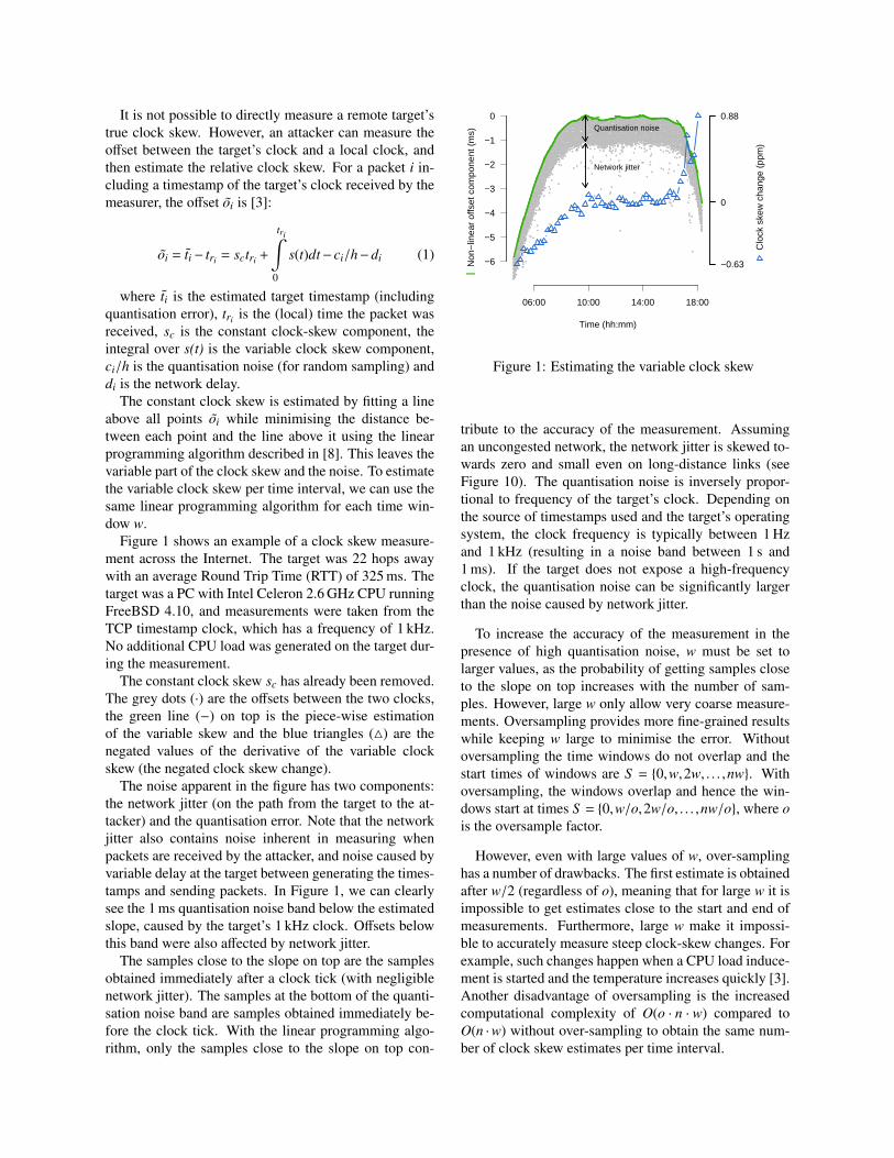
Figure 1 shows an example of a clock skew measure-ment across the Internet. The target was 22 hops awaywith an average Round Trip Time (RTT) of 325 ms. Thetarget was a PC with Intel Celeron 2.6 GHz CPU runningFreeBSD 4.10, and measurements were taken from theTCP timestamp clock, which has a frequency of 1 kHz.No additional CPU load was generated on the target dur-ing the measurement.

The constant clock skew sc has already been removed.The grey dots (·) are the offsets between the two clocks,the green line (−) on top is the piece-wise estimationof the variable skew and the blue triangles (4) are thenegated values of the derivative of the variable clockskew (the negated clock skew change).

The noise apparent in the figure has two components:the network jitter (on the path from the target to the at-tacker) and the quantisation error. Note that the networkjitter also contains noise inherent in measuring whenpackets are received by the attacker, and noise caused byvariable delay at the target between generating the times-tamps and sending packets. In Figure 1, we can clearlysee the 1 ms quantisation noise band below the estimatedslope, caused by the target’s 1 kHz clock. Offsets belowthis band were also affected by network jitter.

The samples close to the slope on top are the samplesobtained immediately after a clock tick (with negligiblenetwork jitter). The samples at the bottom of the quanti-sation noise band are samples obtained immediately be-fore the clock tick. With the linear programming algo-rithm, only the samples close to the slope on top con-

06:00 10:00 14:00 18:00

Time (hh:mm)

Non

−lin

ear

offs

et c

ompo

nent

(m

s)

−−6

−5

−4

−3

−2

−1

0

−0.63

0

0.88

Clo

ck s

kew

cha

nge

(ppm

)

Quantisation noise

Network jitter

sc == 279, min s((t)) == −0.63, max s((t)) == 0.88 ppm

Figure 1: Estimating the variable clock skew

tribute to the accuracy of the measurement. Assumingan uncongested network, the network jitter is skewed to-wards zero and small even on long-distance links (seeFigure 10). The quantisation noise is inversely propor-tional to frequency of the target’s clock. Depending onthe source of timestamps used and the target’s operatingsystem, the clock frequency is typically between 1 Hzand 1 kHz (resulting in a noise band between 1 s and1 ms). If the target does not expose a high-frequencyclock, the quantisation noise can be significantly largerthan the noise caused by network jitter.

To increase the accuracy of the measurement in thepresence of high quantisation noise, w must be set tolarger values, as the probability of getting samples closeto the slope on top increases with the number of sam-ples. However, large w only allow very coarse measure-ments. Oversampling provides more fine-grained resultswhile keeping w large to minimise the error. Withoutoversampling the time windows do not overlap and thestart times of windows are S = {0,w,2w, . . . ,nw}. Withoversampling, the windows overlap and hence the win-dows start at times S = {0,w/o,2w/o, . . . ,nw/o}, where ois the oversample factor.

However, even with large values of w, over-samplinghas a number of drawbacks. The first estimate is obtainedafter w/2 (regardless of o), meaning that for large w it isimpossible to get estimates close to the start and end ofmeasurements. Furthermore, large w make it impossi-ble to accurately measure steep clock-skew changes. Forexample, such changes happen when a CPU load induce-ment is started and the temperature increases quickly [3].Another disadvantage of oversampling is the increasedcomputational complexity of O(o · n · w) compared toO(n ·w) without over-sampling to obtain the same num-ber of clock skew estimates per time interval.

Page 4

3.1 Timestamp SourcesPrevious research used different timestamps sourcesfor clock-skew estimation: ICMP timestamp responses,TCP timestamp header extensions or TCP sequencenumbers [3, 4].

TCP sequence numbers on Linux are the sum of acryptographic result and a 1 MHz clock. They providegood clock-skew estimates over short periods because ofthe high frequency, but re-keying of the cryptographicfunction every five minutes makes longer measurementsnon-trivial [3].

ICMP timestamps have a fixed frequency of 1 kHz.Their disadvantage is that they are affected by clock ad-justments done by the Network Time Protocol (NTP) [9],which makes estimation of variable clock skew more dif-ficult. Furthermore, ICMP messages are now blocked bymany firewalls.

TCP timestamps have a frequency between 1 Hz and1 kHz, depending on the operating system. Their ad-vantage is that they are generated before NTP adjust-ments are made [4]. TCP timestamps are currently thebest option for clock-skew measurement because theyare widely available and unaffected by NTP (at least forLinux, FreeBSD and Windows [4]). However, even TCPtimestamps are not available in all situations. They maynot be enabled on certain operating systems and they can-not be used if there is no end-to-end TCP connection tothe target. For example, they cannot be used through theTor anonymisation network.

HTTP timestamps have a frequency of 1 Hz and areavailable from every web server. However, these havenot been previously used for clock-skew measurementdue to the low frequency. We describe how to exploitthem in the following section.

4 New Attacks

A major disadvantage of the attack in [3] is that the at-tacker needs to exchange large amounts of traffic withthe hidden service across the Tor network in order toaccurately measure clock skew changes. It may not bepossible to actually send sufficient traffic because Tordoes not provide enough bandwidth, or because the ser-vice operator actively limits the request rate to avoidoverload, prevent Denial of Service (DoS) attacks etc.Furthermore, the attack also relies on an exposed high-frequency timestamp source (experiments used the 1 kHzTCP timestamp) on the target for adequate clock-skewestimation.

The synchronised sampling technique proposed in thispaper improves the existing attack reducing the dura-tion and amount of network traffic required. Measur-ing clock-skew requires only a small amount of traf-

fic compared to the amount of traffic needed for loadinducement. For example, the exchange of one re-quest/response every 1.5 s is sufficient for clock-skew es-timation.

Our improvements also make the existing attack ap-plicable in situations where high-resolution timestampsare not available. For example ICMP or TCP times-tamps (see Section 3.1) are not available across Tor, sinceit only supports TCP and streams are re-assembled onthe client, removing any headers. Because our proposedtechnique allows accurate clock-skew estimation fromlow-resolution timestamps, HTTP timestamps obtainedfrom a hidden web server across the Tor network couldbe used. The fact that low-resolution timestamps are us-able opens the door to new variants of the attack.

In the first new attack variant, the attacker measuresthe variable clock skew of the hidden service via Tor, andof all the candidate hosts via accessing the IP addressesdirectly. Then the attacker compares the variable clock-skew pattern of the hidden service with the patterns ofall the candidates. The variable clock skew patterns ofdifferent hosts differ sufficiently over time, and the du-ration of the attack could be increased arbitrarily. Whilethis attack has the benefit of not requiring large amountsof traffic to be exchanged, it could still take a long time.The attacker must ensure that both timestamp sources arederived from the same physical source

A quicker version of this attack could only comparethe fixed clock-skew of the target measured via Tor withthe fixed clock-skew measured directly for all candidates.Kohno et al. showed that clock skew of a particular hostchanges very little over time, but the difference betweendifferent hosts is significant [4].

Another new attack variant is based on the idea of us-ing clock-skew estimates for geo-location [3]. The at-tacker identifies the location of the candidates based ontheir IP addresses and a geo-location database. For ex-ample, GeoLite is a freely available database that mapsIP addresses to locations with a claimed accuracy of over98% [10]. The attacker measures the variable clock skewof the hidden service via Tor. The attacker then estimatesthe location based on the variable clock-skew pattern us-ing the technique described in [3].

This attack works even in cases where the attackercannot access the candidate hosts directly. On the otherhand this attack does not allow an unambiguous identi-fication of the hidden service if candidate locations aregeographically close together.

4.1 Attacking HTTP TimestampsThe key common factor among the new attacks discussedabove is that clock skew must be estimated from re-sponses sent over the hidden service channel. Previ-ous work has not examined this option because typically

Page 5

...

HTTP Client HTTP Server

SYN

SYN+ACK

ACK

GET index.html

HTTP/1.0 200 OK

tri

ti

~~

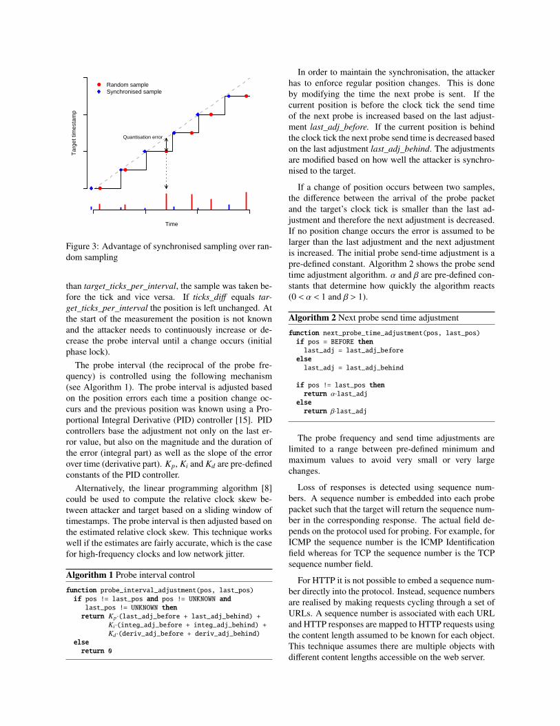
Figure 2: HTTP request/response and the timestampsneeded for clock skew estimation

only a low frequency clock is available and quantisationnoise dominates the small effect of temperature on clockskew. However, in this paper we will show how it isstill possible to exploit this clock. Here, the attacker actsas HTTP client sending minimal HTTP requests to thetarget. Standard web servers include a 1 Hz timestampin the Date header of HTTP responses because it wasrecommended for HTTP 1.0 [11] and is mandatory forHTTP 1.1 (excluding 5xx server errors and some 1xx re-sponses) [12].

Before the HTTP exchange a TCP connection needsto be established between client and server. IncludingTCP connection establishment, it may take at least twofull round trip times from when the client wants to senda request until the response is received. To minimise theTCP overhead, the client should open a TCP connectionbeforehand. Ideally, it should only open the connectiononce and then keep it alive for the duration of the mea-surement. However, it is not possible for a client to forcea server to keep a connection open. Therefore, when theclient notices that the server has closed the connection,it should immediately re-open it. Then, the next HTTPrequest can be sent at the appropriate time determined bythe synchronised sampling algorithm.

The HTTP timestamp is usually generated after theserver has received the client’s request. We verified thatApache 2.2.x generates the timestamp after the requesthas been successfully parsed [13]. The correspondingclient timestamp is the time the packet containing theDate header is received, which is usually the first packetsent by the server after the TCP connection has been fullyestablished (see Figure 2).

5 Implementation

Previous approaches to remote clock-skew estimationhave sampled timestamps at random times. However,

with the 1 Hz HTTP timestamp, the consequent highquantisation noise would prevent the attack from accu-rately measuring the target’s clock skew within a feasibleperiod. Instead, we must probe the target’s clock imme-diately after a clock tick occurred, because here the quan-tisation error is the smallest. To achieve this, the attackerhas to synchronise its probing phase and frequency suchthat probes arrive shortly after the clock tick. We as-sume the attacker selects a nominal sample frequency,based on the desired accuracy and intrusiveness of themeasurement.

The attacker cannot measure the exact time differencebetween the arrival of probe packets and the clock ticks.To maintain synchronisation, the attacker has to alternatebetween sampling before and after the clock tick. Sam-ples before the clock tick can be corrected by adding onetick, as their true value is actually closer to the next clocktick. However, the linear programming algorithm stillcannot use these samples because for them the quantisa-tion error and jitter are in opposite directions and cannotbe separated.

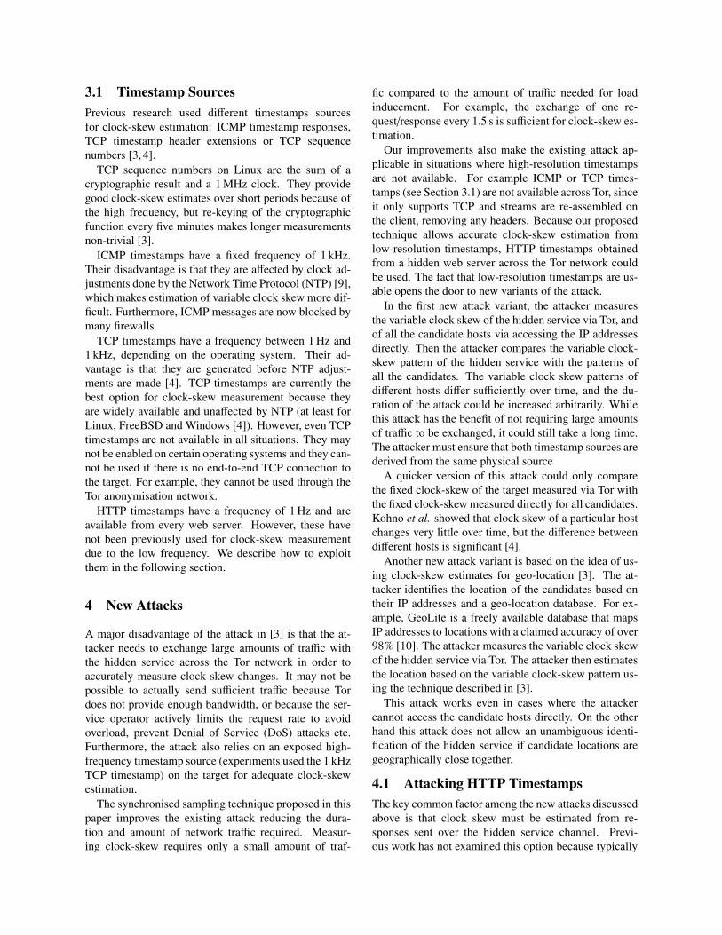
Figure 3 illustrates the benefit of synchronised sam-pling over random sampling. The solid step line is thetarget’s clock value over time and the dashed line showsthe true time. Random samples are distributed uniformlybetween clock ticks whereas synchronised samples aretaken close to the clock ticks. Note that in the figure, thetime for samples before the tick has been corrected asdescribed above. The quantisation errors are the differ-ences between samples’ y-values and the true time. Theabsolute quantisation errors are shown as bars at the bot-tom. Synchronised sampling leads to smaller errors incomparison with random sampling.

Our algorithm is similar to existing Phase Lock Loop(PLL) techniques used for aligning the frequency andphase of a signal with a reference [14]. However,whereas PLL techniques measured the phase differenceof two signals, we can only estimate the phase differenceby detecting whether a sample was taken before or afterthe clock tick.

5.1 AlgorithmInitially, the attacker starts probing with the nominalsample frequency and measures how many clock ticksoccur in one sample interval (target_ticks_per_interval).The measurement is repeated to obtain the correct num-ber of ticks.

The attacker cannot measure the exact time differencebetween the arrival of a probe packet and the target’sclock tick. However, the attacker can measure the po-sition of the probe arrival relative to the target’s clocktick based on the number of clock ticks that occurredbetween the current and the last timestamp of the tar-get (ticks_diff ). If the number of clock ticks is less

Page 6

Time

Tar

get t

imes

tam

p

●

●

●

●

●

●

Quantisation error

● Random sampleSynchronised sample

Figure 3: Advantage of synchronised sampling over ran-dom sampling

than target_ticks_per_interval, the sample was taken be-fore the tick and vice versa. If ticks_diff equals tar-get_ticks_per_interval the position is left unchanged. Atthe start of the measurement the position is not knownand the attacker needs to continuously increase or de-crease the probe interval until a change occurs (initialphase lock).

The probe interval (the reciprocal of the probe fre-quency) is controlled using the following mechanism(see Algorithm 1). The probe interval is adjusted basedon the position errors each time a position change oc-curs and the previous position was known using a Pro-portional Integral Derivative (PID) controller [15]. PIDcontrollers base the adjustment not only on the last er-ror value, but also on the magnitude and the duration ofthe error (integral part) as well as the slope of the errorover time (derivative part). Kp, Ki and Kd are pre-definedconstants of the PID controller.

Alternatively, the linear programming algorithm [8]could be used to compute the relative clock skew be-tween attacker and target based on a sliding window oftimestamps. The probe interval is then adjusted based onthe estimated relative clock skew. This technique workswell if the estimates are fairly accurate, which is the casefor high-frequency clocks and low network jitter.

Algorithm 1 Probe interval control

function probe_interval_adjustment(pos, last_pos)if pos != last_pos and pos != UNKNOWN andlast_pos != UNKNOWN thenreturn Kp·(last_adj_before + last_adj_behind) +

Ki·(integ_adj_before + integ_adj_behind) +Kd ·(deriv_adj_before + deriv_adj_behind)

elsereturn 0

In order to maintain the synchronisation, the attackerhas to enforce regular position changes. This is doneby modifying the time the next probe is sent. If thecurrent position is before the clock tick the send timeof the next probe is increased based on the last adjust-ment last_adj_before. If the current position is behindthe clock tick the next probe send time is decreased basedon the last adjustment last_adj_behind. The adjustmentsare modified based on how well the attacker is synchro-nised to the target.

If a change of position occurs between two samples,the difference between the arrival of the probe packetand the target’s clock tick is smaller than the last ad-justment and therefore the next adjustment is decreased.If no position change occurs the error is assumed to belarger than the last adjustment and the next adjustmentis increased. The initial probe send-time adjustment is apre-defined constant. Algorithm 2 shows the probe sendtime adjustment algorithm. α and β are pre-defined con-stants that determine how quickly the algorithm reacts(0 < α < 1 and β > 1).

Algorithm 2 Next probe send time adjustment

function next_probe_time_adjustment(pos, last_pos)if pos = BEFORE thenlast_adj = last_adj_before

elselast_adj = last_adj_behind

if pos != last_pos thenreturn α·last_adj

elsereturn β·last_adj

The probe frequency and send time adjustments arelimited to a range between pre-defined minimum andmaximum values to avoid very small or very largechanges.

Loss of responses is detected using sequence num-bers. A sequence number is embedded into each probepacket such that the target will return the sequence num-ber in the corresponding response. The actual field de-pends on the protocol used for probing. For example, forICMP the sequence number is the ICMP Identificationfield whereas for TCP the sequence number is the TCPsequence number field.

For HTTP it is not possible to embed a sequence num-ber directly into the protocol. Instead, sequence numbersare realised by making requests cycling through a set ofURLs. A sequence number is associated with each URLand HTTP responses are mapped to HTTP requests usingthe content length assumed to be known for each object.This technique assumes there are multiple objects withdifferent content lengths accessible on the web server.

Page 7

If packet loss is detected, the algorithm adjuststicks_diff by subtracting the number of lost packet mul-tiplied by target_ticks_per_interval. Reordered packetsare considered lost.

Algorithm 3 shows the synchronisation procedure.Our algorithm works with different timestamps and dif-ferent clock frequencies. It has been tested with ICMP,TCP and HTTP timestamps and TCP clock frequenciesof 100 Hz, 250 Hz and 1 kHz.

Algorithm 3 Synchronised sampling

foreach response_packet dodiff = target_timestamp - last_target_timestamp

if target_ticks_per_interval == -1 thenpos = UNKOWNtarget_ticks_per_interval = ticks_diff

else if ticks_diff > target_ticks_per_interval thenpos = BEHIND

else if ticks_diff < target_ticks_per_interval thenpos = BEFORE

elsepos = last_pos

probe_interval = probe_interval +probe_interval_adjustment(pos, last_pos)

probe_time = last_probe_time + probe_interval +next_probe_time_adjustment(pos, last_pos)

last_pos = poslast_target_timestamp = target_timestamplast_probe_time = probe_time

5.2 Errors

Any constant delay does not affect the synchronisationprocess. However, changes in delay on the path fromthe attacker to the target will affect the arrival time ofthe probe packets. This could be caused by jitter in thesending process (jitter inside the attacker), network jitter(queuing delays in routers) or jitter in the target’s packetreceiving process.

Often we can assume the network is uncongested andtherefore network jitter is skewed towards zero. Thisis usually the case in a LAN (see Section 6). Even onthe Internet many links are not heavily utilised and pathchanges (caused by routing changes) are usually infre-quent. Load-balancing is usually performed on a per-flow basis to eliminate any negative impacts on TCP andUDP performance.

However, when measuring clock skew over a Tor cir-cuit we expect much higher network jitter. A Tor cir-cuit is composed of a number of network connectionsbetween different nodes. The overall jitter does not onlyinclude the jitter of each connection but also the jitter in-troduced by the Tor nodes themselves.

The timing of sending probes is not very exact if thesender is a userspace application. Even if the userspacesend() system call is called at the appropriate time, therewill be a delay before the packet is actually sent ontothe physical medium. The variable part of this delay cancause probe packets to arrive too late or too early. Thiserror could be reduced by running the software entirelyin the kernel (e.g. as kernel module), using a real-timeoperating system or by using special network cards sup-porting very precise sending of packets. Any variabledelay in the packet receiving process of the target hasthe same effect and is unfortunately out of control of theattacker. The only way an attacker could reduce such er-rors would be to adjust the sending of the probe packetsbased on a prediction of the jitter inside the target, whichappears to be a challenging task.

Another error is introduced when the relative clockskew between attacker and target changes and the algo-rithms needs to adjust the probe frequency. The attackeris able to control its time keeping and avoid any suddenclock changes. But if the target is running NTP and thetimestamps are affected by NTP adjustments, changes inrelative clock skew are possible.

6 Evaluation

In the first part of this section we compare the accuracy ofsynchronised and random sampling in a LAN testbed us-ing TCP timestamps with typical target clock frequenciesof 100 Hz, 250 Hz and 1000 Hz, as well as 1 Hz HTTPtimestamps. Since in the LAN network jitter is negligi-ble the results show the maximum improvement of usingsynchronised sampling and demonstrate that our imple-mentation is working correctly.

In the second part we compare the accuracy of syn-chronised and random sampling based on TCP times-tamps across a 22-hop Internet path. The result showsthat even on a long path, synchronised sampling signif-icantly increases clock-skew estimation accuracy, whichimproves on the attack proposed by Murdoch [3].

In the third part we compare the accuracy of synchro-nised and random sampling for probing a web server run-ning as a Tor hidden service. We show that synchronisedsampling improves clock skew estimation significantly,even over a path with high network jitter. We also showthat a hidden web sever can be identified among a can-didate set by comparing the variable clock skew overtime using synchronised sampling. Furthermore, usingsynchronised sampling shows daily temperature patternsthat could not be identified using random sampling.

Finally, we investigate how long our technique needsfor the initial synchronisation (the time until the attackerhas locked on to the phase and frequency of the target’sclock ticks). We compare the times for HTTP probing

Page 8

in a LAN and probing a hidden web server over a Tornetwork.

To evaluate the accuracy of synchronised and randomsampling we need to know the true values of the variableclock skew. Since it is impossible to directly measurethis, we use the following approach. In our tests the tar-get also runs a UDP server and the attacker runs a UDPclient. The UDP client sends requests to the server at reg-ular time intervals. Upon receiving a request, the UDPserver returns a packet with a timestamp set to the sendtime of the response. The UDP client records the time itreceives the response.

We compute the offset between the two timestamp-series and estimate the variable clock skew as usual.Since the UDP-based timestamp has a precision of 1 µs,the quantisation error is negligible. Although these UDPestimates are not the true values of the variable clockskew we use them as baseline for synchronised and ran-dom sampling, which have much higher quantisation er-rors. In the following we refer to this as UDP probing orUDP measurement.

A drawback of our current implementation is that theUDP server is a userspace program. The server’s re-sponse timestamp is taken in userspace before the re-sponse packet is sent via the sendto() system call. Toreduce these timing errors one could implement a kernel-based version of the UDP server.

We compare the variable skew estimates for synchro-nised and random sampling with the reference values,from the UDP measurement, using the root mean squareerror (RMSE) of the data values x against the referencevalues x:

RMS E =

√1N

∑i

(xi− xi)2. (2)

We also compute histograms of the noise band for syn-chronised and random sampling. The noise is definedas difference between the variable clock offset and theUDP timestamp estimated variable skew. For randomsampling the quantisation noise band is always uniformwith width 1/ f , where f is the clock frequency. For syn-chronised sampling the quantisation noise depends onhow well the synchronised sampling algorithm is able totrack the target’s clock tick. For synchronised samplingthe noise is given by the samples taken after the clocktick because only these samples are used to estimate theclock skew.

In all experiments we set α = 0.5 and β = 1.5. ForTCP timestamps the linear programming algorithm wasused to adjust the probe interval with a sliding window ofsize 120 (LAN) and 300 (Internet). For HTTP timestampmeasurements the probe interval was adjusted using the

PID controller with Kp = 0.09, Ki = 0.0026 and Kd =

0.02.

6.1 Synchronised vs. Random Sampling inLAN Environments

The attacker was a PC with Intel Xeon 3.6 GHz Quad-Core CPU running Linux 2.6. The target was a PC withIntel Xeon 3.6 GHz Quad-Core CPU running Linux 2.6with a TCP timestamp frequency of 1 kHz. Attacker andtarget were connected to the same Ethernet switch. Theattacker simultaneously performed synchronised, ran-dom and UDP probing. Synchronised and random prob-ing had an average sampling period of 1.5 s, the same rateas in [3]. The UDP probing was performed with a fastersample rate of 1 s in order to achieve a higher accuracyfor the reference measurement. A second UDP measure-ment with an average sample rate of 1 s was run in orderto investigate the error between UDP measurements. Theduration of the test was approximately 24 hours.

As the test was run inside a LAN the average RTT wasonly 130 µs and the RTT / 2 jitter was small with a max-imum of 60 µs and a median of 30 µs. Figure 4 showshistograms of the noise bands of synchronised and ran-dom sampling with respect to the reference given by theUDP measurement. For synchronised sampling most ofthe offsets are within 100 µs whereas for random sam-pling we see the expected 1 ms noise band.

In Figure 5 we compare the RMSE of synchronisedsampling, random sampling and the second UDP mea-surement for different window sizes against the UDP ref-erence with maximum window size (1800 s). We alsocompare the UDP reference against itself at smaller win-dow sizes. The oversampling factor was chosen such thatthe time between two clock-skew estimates is the sameregardless of the window size (30 s). This has the advan-tage of providing approximately the same number of es-timates for all window sizes. (For smaller window sizesthere are still more samples, because there are samplescloser to the start and end of the measurement period.)

Figure 5 shows that synchronised sampling performssignificantly better than random sampling. There is a dif-ference between the second UDP measurement and theUDP reference, but it is smaller than the difference be-tween synchronised sampling and the UDP reference forall window sizes. Hence we conclude the error of UDPmeasurements is sufficiently small for using it as base-line. In the later experiments we performed only oneUDP measurement.

The target clock frequency was 1 kHz, which is themaximum TCP timestamp frequency of current operat-ing systems. However, it is likely that in reality manyhosts actually have lower TCP clock frequencies. For ex-ample, 100 Hz is the clock frequency used by older Linux

Page 9

Median: 0.04 ms

Noise (ms)

Den

sity

0

5

10

15

20

0.00 0.05 0.10 0.15

Median: 0.51 ms

Noise (ms)

Den

sity

0.0

0.2

0.4

0.6

0.8

1.0

0.0 0.2 0.4 0.6 0.8 1.0

Figure 4: Noise distributions in LAN: synchronised sampling (left) vs. random sampling (right)

●

●

●

●

●

●●

●

0 500 1000 1500

0.005

0.010

0.020

0.050

0.100

0.200

0.500

1.000

2.000

Window size (s)

40 200 400 600 800 1200

RM

SE

(pp

m)

Avg. samples per window (sync & random)

●

●

●

●

●

●●

●

●

ReferenceSyncRandomUDP

Figure 5: RMSE of synchronised, random sampling andUDP reference in LAN with a target clock frequency of1 kHz (log y-axis)

●

●

●

●

●

●●

●

0 500 1000 1500

Window size (s)

40 200 400 600 800 1200

RM

SE

(pp

m)

0.0050.010

0.0500.100

0.5001.000

5.00010.000

Avg. samples per window (sync & random)

●

●

●

●

●

●●

●

●

●

●

●

●

●

●

●

●

●

Sync 100 HzSync 250 HzSync 1000 HzRandom 100 HzRandom 250 HzRandom 1000 Hz

Figure 6: RMSE of synchronised and random samplingfor different clock frequencies of 100 Hz, 250 Hz and1 kHz against the same target. Different clock frequen-cies were obtained by rounding the target timestamps im-mediately after reception (log y-axis)

and FreeBSD kernels and 250 Hz is the clock frequencyof modern Linux 2.6 kernels.

To evaluate the RMSE for lower clock frequencies weused the same setup. This time we ran three synchronisedand three random probing processes simultaneously for24 hours, rounding the target timestamps so that we ef-fectively measured 100 Hz, 250 Hz and 1 kHz clocks.Figure 6 shows the RMSE for synchronised and randomsampling for the different target clock frequencies. TheUDP measurement has been omitted for better readabil-ity. The graph shows that the accuracy of synchronisedsampling does not depend on the clock frequency andthe RMSE for random sampling increases significantlyfor lower clock frequencies.

In another LAN experiment we ran a web server(Apache 2.2.4) on the target and the attacker used HTTP

probing. The average sampling interval was 2 s, becausethis is the minimum probe frequency for 1 Hz HTTPtimestamps. The web server was completely idle (exceptfor the requests generated by the attacker). The durationof the experiment was approximately 24 hours.

Although the experiment was carried out between thesame two hosts as before, the RTT / 2 jitter was higherwith a maximum of 120 µs and a median of 60 µs. Theweb server running in userspace introduced the addi-tional jitter. Figure 7 shows the noise for synchronisedsampling and random sampling. For synchronised sam-pling the noise band is only slightly larger than in Figure4. Because of the higher jitter, the synchronisation is lessaccurate. For random sampling the noise band is 1 s be-cause of the 1 Hz HTTP clock frequency.

Page 10

Median: 0.06 ms

Noise (ms)

Den

sity

0

2

4

6

8

10

12

0.0 0.1 0.2 0.3 0.4 0.5 0.6 0.7

Median: 501.12 ms

Noise (ms)

Den

sity

0e+00

2e−04

4e−04

6e−04

8e−04

1e−03

0 200 400 600 800 1000

Figure 7: Noise distributions for HTTP probing in LAN: synchronised sampling (left) vs. random sampling (right)

●

●●

●

●●

●●

0 500 1000 1500

Window size (s)

0.01

0.10

1.00

10.00

100.00

1000.00

30 150 300 450 600 900

RM

SE

(pp

m)

Avg. samples per window (sync & random)

●

●●

●

●●

●●

●

ReferenceSyncRandom

Figure 8: RMSE of synchronised sampling, random sam-pling and the UDP measurement for HTTP probing inLAN

Figure 8 shows the RMSE of synchronised sampling,random sampling and the UDP measurement against thereference at maximum window size. The RMSEs of syn-chronised sampling and UDP reference are very similarto the results in Figure 5. Because of the large noiseband, the RMSE for random sampling is more than twoorders of magnitude above the RMSE for synchronisedsampling. This demonstrates that our new algorithm isable to effectively measure clock skew changes for lowfrequency clocks, an infeasible task for random sam-pling.

6.2 Synchronised vs. Random SamplingAcross Internet Paths

The attacker was the same machine as in Section 6.1located in Cambridge, UK. The target was 22 hopsaway located in Canberra, Australia. The target was aFreeBSD 4.10 PC with a kernel tick rate set to 1000 and

therefore the TCP timestamp frequency was 1 kHz. Theaverage RTT between measurer and target was 325 ms.The duration of the measurement was approximately 21hours. We performed synchronised, random and UDPprobing.

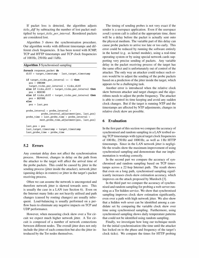
Despite the high RTT, the jitter is small and skewedtowards zero as shown in Figure 10. Figure 9 showshistograms of the noise bands of synchronised and ran-dom sampling in relation to the reference given by theUDP measurement. For synchronised sampling most ofthe offsets are within 250 µs of the reference whereas forrandom sampling there is the expected 1 ms noise band.

Figure 11 shows the RMSE of synchronised sampling,random sampling and the UDP reference against theUDP reference at maximum window size using the sameparameters as in Section 6.1. The gain of synchronisedsampling is smaller compared to Section 6.1 because ofthe higher network jitter but still significant for smallerwindow sizes.

6.3 Attacking Tor Hidden ServicesFor our measurements we used a private Tor network.Our Tor nodes are distributed across the Internet runningon Planetlab [16] nodes. The main reason for using a pri-vate Tor network instead of the public Tor network is thepoor performance of hidden services in the public Tornetwork. Besides huge network jitter that prevents anyaccurate clock-skew measurements, hidden services al-ways disappeared after few hours preventing longer mea-surements. While currently it is difficult to carry out theattack in the public Tor network, it should become easierin the future, as the Tor team is now working on improv-ing the performance of hidden services.

We selected 18 Planetlab widely geographically dis-tributed nodes on which we ran Tor nodes (of which3 were directory authorities). We selected nodes thathad low CPU utilisation at the time of selection. AnIntel Core2 2.4 GHz with 4 GB RAM running Linux

Page 11

Median: 0.12 ms

Noise (ms)

Den

sity

0

1

2

3

4

5

0.0 0.5 1.0 1.5 2.0

Median: 0.53 ms

Noise (ms)

Den

sity

0.0

0.2

0.4

0.6

0.8

1.0

0.0 0.5 1.0 1.5 2.0 2.5

Figure 9: Noise distributions for Internet path: synchronised sampling (left) vs. random sampling (right)

Median: 0.04 ms

RTT jitter / 2 (ms)

Den

sity

0

2

4

6

8

10

12

0.0 0.2 0.4 0.6 0.8 1.0 1.2

Figure 10: RTT jitter / 2 on path across the Internet

●

●

●

●

●●

●●

0 500 1000 1500

0.01

0.02

0.05

0.10

0.20

0.50

1.00

2.00

Window size (s)

40 200 400 600 800 1200

RM

SE

(pp

m)

Avg. samples per window (sync & random)

●

●

●

●

●●

●●

●

ReferenceSyncRandom

Figure 11: RMSE of synchronised sampling and randomsampling for different window sizes measured across In-ternet path.

2.6.16 was used to run another Tor node and the hiddenweb server. No load is induced on the server, so anyclock skew changes are based on the ambient tempera-ture changes.

An Intel Celeron 2.4 GHz with 1.2 GB of RAM run-ning Linux 2.6.16 was used to run a Tor client and ourprobe tool. We used tsocks [17] with the latest Tor re-lated patches to enable our tool to interact with the Torclient via the SOCKS protocol and to properly handleTor hidden server pseudonyms.

First we performed an experiment similar to the onesin Section 6.1 and Section 6.2. Synchronised and randomsampling was performed across the Tor network, whileUDP probing was performed directly between the clientmachine and the hidden server. The measurement dura-tion was approximately 18 hours.

The average RTT between client and hidden serveracross Tor was 885 ms. Figure 14 shows the RTT / 2

jitter, which is considerably higher than in the previ-ous measurements. Figure 12 shows histograms of thenoise bands of synchronised and random sampling. Forrandom sampling it shows the expected 1 s noise band.For synchronised sampling the noise is greatly reduced.Most of the offsets are ≤ 100 ms away from the slopegiven by the UDP reference.

Figure 13 shows the change of clock skew for synchro-nised sampling as blue squares (�) and random samplingas red circles (�) and the UDP reference as black line(−) for a window size of 1800 s and 2 hours. The noiseis much smaller for synchronised sampling compared torandom sampling especially for small window sizes. Fora window size of 2 hours one can clearly see a daily tem-perature change of the reference curve with the temper-ature (and hence the clock skew) dropping during nighthours and suddenly increasing in the morning. The syn-chronised sampling curve shows the same pattern with

Page 12

Median: 10.44 ms

Noise (ms)

Den

sity

0.00

0.01

0.02

0.03

0.04

0 100 200 300 400 500 600

Median: 517.24 ms

Noise (ms)

Den

sity

0.0000

0.0002

0.0004

0.0006

0.0008

0.0010

0.0012

0 200 400 600 800 1000 1200

Figure 12: Noise distributions Planetlab Tor testbed: synchronised sampling (left) vs. random sampling (right)

●

●●●●

●

●●

●

●

●●

●

●

●

●●

●●●●

●

●●

●●●

●

●

●●●●

●

●

●●

●●

●●

●●●●●●●●

●●●●

●

●

●

●

●●●

●

●●

●●

●

●●

●●

●

●●●

●

●

●●●

●●

●

●

●

●●●

●●

●●●●●●

●●

●●●

●

●

●●●●●

●●

●

●●

●

●●●

●●

●●

●

●

●

●

●

●●

●

●●

●

●

●●●

●●●●

●

●

●●

●●●

●

●

●

●●

●

●●

●

●●●●

●

●

●

●●

●

●

●●●●

●●

●

●●

●

●

●●

●

●●

●

●●

●

●

●●●

●

●●●

●●●

●●●●

●

●●●●●

●●

●●●

●

●●●

●

●●●●

●

●●

●

●

●

●

●

●●●

●

●●

●

●

●

●●

●

●

●●

●●●●●●●●

●●

●●

●●

●

●●●

●

●●●●●●

●●

●

●●

●●

●

●

●●

●●

●●

●

●

●●

●

●●

●●

●

●

●●

●●

●●

●●●

●

●●

●●●

●●●

●

●

●●●●●

●●

●●

●

●

●●●●

●

●●●●●●●●●

●●

−20

0

20

40

Window size: 1800 s

Time (mm:ss)

Clo

ck s

kew

cha

nge

(ppm

)

15:00 19:00 23:00 03:00 07:00

●

●●●●

●

●●

●

●

●●

●

●

●

●●

●●●●

●

●●

●●●

●

●

●●●●

●

●

●●

●●

●●

●●●●●●●●

●●●●

●

●

●

●

●●●

●

●●

●●

●

●●

●●

●

●●●

●

●

●●●

●●

●

●

●

●●●

●●

●●●●●●

●●

●●●

●

●

●●●●●

●●

●

●●

●

●●●

●●

●●

●

●

●

●

●

●●

●

●●

●

●

●●●

●●●●

●

●

●●

●●●

●

●

●

●●

●

●●

●

●●●●

●

●

●

●●

●

●

●●●●

●●

●

●●

●

●

●●

●

●●

●

●●

●

●

●●●

●

●●●

●●●

●●●●

●

●●●●●

●●

●●●

●

●●●

●

●●●●

●

●●

●

●

●

●

●

●●●

●

●●

●

●

●

●●

●

●

●●

●●●●●●●●

●●

●●

●●

●

●●●

●

●●●●●●

●●

●

●●

●●

●

●

●●

●●

●●

●

●

●●

●

●●

●●

●

●

●●

●●

●●

●●●

●

●●

●●●

●●●

●

●

●●●●●

●●

●●

●

●

●●●●

●

●●●●●●●●●

●●

●Reference Sync Random

●●●

●●●●●●●

●

●

●●●●●

●●

●●●

●●

●

●●●

●●

●●

●●

●●●●●

●

●●

●●●●●

●●●●

●●

●●●

●●●●

●●●●

●●●●●

●●●

●●

●●●

●●

●●

●●

●●●●●●

●●

●●

●●●●●●

●●

●●●●

●

●●●

●●●

●●

●●●●●

●

●●●●●●●

●●

●●●

●●●●●

●●

●●

●●●●●

●●

●

●●

●●●●

−2

−1

0

1

2

Window size: 7200 s

Time (mm:ss)

Clo

ck s

kew

cha

nge

(ppm

)

15:00 19:00 23:00 03:00 07:00

●●●

●●●●●●●

●

●

●●●●●

●●

●●●

●●

●

●●●

●●

●●

●●

●●●●●

●

●●

●●●●●

●●●●

●●

●●●

●●●●

●●●●

●●●●●

●●●

●●

●●●

●●

●●

●●

●●●●●●

●●

●●

●●●●●●

●●

●●●●

●

●●●

●●●

●●

●●●●●

●

●●●●●●●

●●

●●●

●●●●●

●●

●●

●●●●●

●●

●

●●

●●●●

●Reference Sync Random

Figure 13: Estimated clock skew changes for hidden service in Planetlab Tor network for a window size of 1800 s(left) and 2 hours (right)

added noise. An attacker could use such daily tempera-ture patterns to estimate the location of the target basedon geo-location. In contrast to random sampling, the pat-tern is not clearly visible because of the much highernoise.

In Figure 15 we compare the RMSE of synchro-nised sampling, random sampling and the UDP referenceagainst the UDP reference at maximum window size.The RMSE of synchronised sampling is almost one mag-nitude lower than the RMSE for random sampling evenfor window sizes as large as two hours.

In the second experiment we performed the actual at-tack. We treated all 19 Tor nodes as candidates and mea-sured their clock skew directly using TCP timestamps(synchronised sampling). At the same time we measuredthe clock skew of the hidden web service via Tor basedon HTTP timestamps using synchronised and randomsampling simultaneously. The experiment lasted about

ten hours. One of the nodes stopped responding in themiddle of the experiment.

Figure 16 shows the RMSE of the HTTP clock skewestimates obtained from the hidden service via Tor us-ing random sampling or synchronised sampling and TCPclock skew estimates of all candidate nodes. We used awindow size of three hours and set the oversample factorso one clock estimate is obtained every 30 s. (For smallerwindows random sampling was not able to consistentlyselect one candidate as the best and would alternate be-tween a few including the correct one for the whole du-ration of the measurement.)

The RMSE of the HTTP timestamp estimate and thecorrect candidate is shown as thick grey (red on colourdisplay) line while RMSEs for all other candidates areshown as thin black lines.

The RMSE between the synchronised sampling Tormeasurement and the direct measurement of the correctcandidate is very small, and with increasing duration be-

Page 13

Median: 6.06 ms

RTT jitter / 2 (ms)

Den

sity

0.00

0.02

0.04

0.06

0.08

0 50 100 150 200

Figure 14: RTT jitter / 2 over Planetlab Tor testbed

●

●●

●

●

●

●

●

●

●●

0 2000 4000 6000 8000 10000

Window size (s)

0.1

1.0

10.0

100.0

1000.0

30 600 1800 3600 5400

RM

SE

(pp

m)

Avg. samples per window (sync & random)

●

●●

●

●

●

●

●

●

●●

●

ReferenceSyncRandom

Figure 15: RMSE of synchronised, random sampling andUDP reference for hidden web service in Planetlab Tornetwork (log y-axis)

0 100 200 300 400 500

0.0

0.2

0.4

0.6

0.8

1.0

Time (min)

RM

SE

(pp

m)

OthersCorrect

0 100 200 300 400 500

0.0

0.2

0.4

0.6

0.8

1.0

Time (min)

RM

SE

(pp

m)

OthersCorrect

Figure 16: RMSE of HTTP clock skew estimates obtained from hidden service via Tor using random sampling (left)or synchronised sampling (right) and TCP clock skew estimates of all candidate nodes

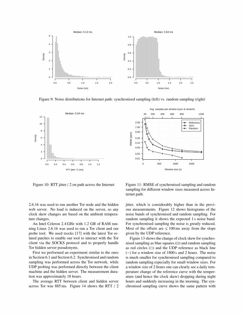
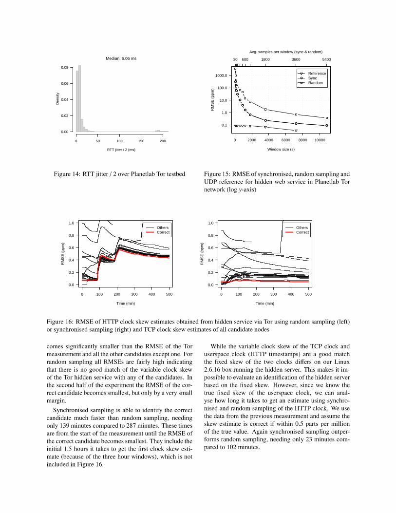
comes significantly smaller than the RMSE of the Tormeasurement and all the other candidates except one. Forrandom sampling all RMSEs are fairly high indicatingthat there is no good match of the variable clock skewof the Tor hidden service with any of the candidates. Inthe second half of the experiment the RMSE of the cor-rect candidate becomes smallest, but only by a very smallmargin.

Synchronised sampling is able to identify the correctcandidate much faster than random sampling, needingonly 139 minutes compared to 287 minutes. These timesare from the start of the measurement until the RMSE ofthe correct candidate becomes smallest. They include theinitial 1.5 hours it takes to get the first clock skew esti-mate (because of the three hour windows), which is notincluded in Figure 16.

While the variable clock skew of the TCP clock anduserspace clock (HTTP timestamps) are a good matchthe fixed skew of the two clocks differs on our Linux2.6.16 box running the hidden server. This makes it im-possible to evaluate an identification of the hidden serverbased on the fixed skew. However, since we know thetrue fixed skew of the userspace clock, we can anal-yse how long it takes to get an estimate using synchro-nised and random sampling of the HTTP clock. We usethe data from the previous measurement and assume theskew estimate is correct if within 0.5 parts per millionof the true value. Again synchronised sampling outper-forms random sampling, needing only 23 minutes com-pared to 102 minutes.

Page 14

0 200 400 600 800 1000

−10

−5

0

5

10

Clock sample

Adj

ust b

efor

e/be

hind

(m

s)

−1000

−500

0

500

1000

Adj

ust i

nter

val (

µµs)

BeforeBehindInterval

0 200 400 600 800 1000

−10

−5

0

5

10

Clock sample

Adj

ust b

efor

e/be

hind

(m

s)

−1000

−500

0

500

1000

Adj

ust i

nter

val (

µµs)

BeforeBehindInterval

Figure 17: Initial synchronisation for HTTP probing in LAN (left) and probing a hidden web server over the Tornetwork (right)

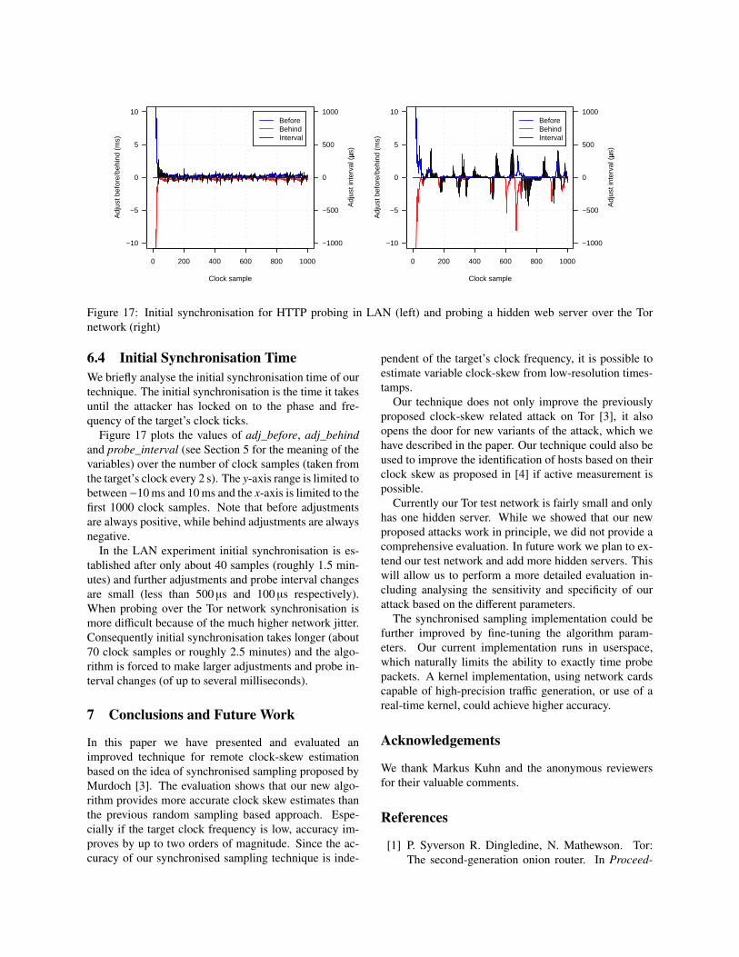
6.4 Initial Synchronisation TimeWe briefly analyse the initial synchronisation time of ourtechnique. The initial synchronisation is the time it takesuntil the attacker has locked on to the phase and fre-quency of the target’s clock ticks.

Figure 17 plots the values of adj_before, adj_behindand probe_interval (see Section 5 for the meaning of thevariables) over the number of clock samples (taken fromthe target’s clock every 2 s). The y-axis range is limited tobetween −10 ms and 10 ms and the x-axis is limited to thefirst 1000 clock samples. Note that before adjustmentsare always positive, while behind adjustments are alwaysnegative.

In the LAN experiment initial synchronisation is es-tablished after only about 40 samples (roughly 1.5 min-utes) and further adjustments and probe interval changesare small (less than 500 µs and 100 µs respectively).When probing over the Tor network synchronisation ismore difficult because of the much higher network jitter.Consequently initial synchronisation takes longer (about70 clock samples or roughly 2.5 minutes) and the algo-rithm is forced to make larger adjustments and probe in-terval changes (of up to several milliseconds).

7 Conclusions and Future Work

In this paper we have presented and evaluated animproved technique for remote clock-skew estimationbased on the idea of synchronised sampling proposed byMurdoch [3]. The evaluation shows that our new algo-rithm provides more accurate clock skew estimates thanthe previous random sampling based approach. Espe-cially if the target clock frequency is low, accuracy im-proves by up to two orders of magnitude. Since the ac-curacy of our synchronised sampling technique is inde-

pendent of the target’s clock frequency, it is possible toestimate variable clock-skew from low-resolution times-tamps.

Our technique does not only improve the previouslyproposed clock-skew related attack on Tor [3], it alsoopens the door for new variants of the attack, which wehave described in the paper. Our technique could also beused to improve the identification of hosts based on theirclock skew as proposed in [4] if active measurement ispossible.

Currently our Tor test network is fairly small and onlyhas one hidden server. While we showed that our newproposed attacks work in principle, we did not provide acomprehensive evaluation. In future work we plan to ex-tend our test network and add more hidden servers. Thiswill allow us to perform a more detailed evaluation in-cluding analysing the sensitivity and specificity of ourattack based on the different parameters.

The synchronised sampling implementation could befurther improved by fine-tuning the algorithm param-eters. Our current implementation runs in userspace,which naturally limits the ability to exactly time probepackets. A kernel implementation, using network cardscapable of high-precision traffic generation, or use of areal-time kernel, could achieve higher accuracy.

Acknowledgements

We thank Markus Kuhn and the anonymous reviewersfor their valuable comments.

References

[1] P. Syverson R. Dingledine, N. Mathewson. Tor:The second-generation onion router. In Proceed-

Page 15

ings of the 13th USENIX Security Symposium, Au-gust 2004.

[2] Reporters Without Borders. Blogger and docu-mentary filmmaker held for the past month, March2006. http://www.rsf.org/article.php3?id_article=16810.

[3] S. J. Murdoch. Hot or not: Revealing hidden ser-vices by their clock skew. In CCS ’06: Proceed-ings of the 9th ACM Conference on Computer andCommunications Security, pages 27–36, Alexan-dria, VA, US, October 2006. ACM Press.

[4] T. Kohno, A. Broido, and kc claffy. Remote phys-ical device fingerprinting. In Proceedings of IEEESymposium on Security and Privacy, pages 211–225, May 2005.

[5] David M. Goldschlag, Michael G. Reed, and Paul F.Syverson. Onion routing. Communications of theACM, 42(2):39–41, February 1999.

[6] Lasse Øverlier and Paul F. Syverson. Locating hid-den servers. In IEEE Symposium on Security andPrivacy, pages 100–114, Oakland, CA, US, May2006. IEEE Computer Society.

[7] Steven J. Murdoch and George Danezis. Low-costtraffic analysis of Tor. In IEEE Symposium on Se-curity and Privacy, pages 183–195, Oakland, CA,US, May 2005. IEEE Computer Society.

[8] D. Towsley S. B. Moon, P. Kelly. Estimation andremoval of clock skew from network delay mea-surements. Technical Report 98-43, Department ofComputer Science, University of Massachussetts atAmherst, October 1998.

[9] D. Mills. Network Time Protocol (Version 3) Spec-ification, Implementation. 1305, IETF, March1992. http://www.ietf.org/rfc/rfc1305.txt.

[10] MaxMind. GeoLite Country, 2008. http://www.maxmind.com/app/geoip_country.

[11] T. Berners-Lee, R. Fielding, and H. Frystyk. Hy-pertext Transfer Protocol – HTTP/1.0. 1945,IETF, May 1996. http://www.ietf.org/rfc/rfc1945.txt.

[12] R. Fielding, J. Gettys, J. Mogul, H. Frystyk,L. Masinter, P. Leach, and T. Berners-Lee. Hy-pertext Transfer Protocol – HTTP/1.1. 2616,IETF, June 1999. http://www.ietf.org/rfc/rfc2616.txt.

[13] Apache Software Foundation. Apache web server.http://www.apache.org/.

[14] C. Langton. Unlocking the phase lock loop -part 1, 2002. http://www.complextoreal.com/chapters/pll.pdf.

[15] Carnegie Mellon University. Pid tutorial.http://www.engin.umich.edu/group/ctm/PID/PID.html.

[16] Brent Chun, David Culler, Timothy Roscoe, AndyBavier, Larry Peterson, Mike Wawrzoniak, and MicBowman. PlanetLab: An overlay testbed for broad-coverage services. ACM SIGCOMM ComputerCommunication Review, 33(3), July 2003.

[17] S. Clowes. Tsocks - a transparent socks proxyinglibrary. http://tsocks.sourceforge.net/.