An iconic position estimator for a 2D laser rangefinder

An Iconic Position Estimator for a 2-D Laser Rangefinder

Javier Gonded, Anthony Steotz, Anibal Ollero'

CMU-RI-TR-92-04

The Robotia Institute Carnegie Mellon University

Pittsburgh. Pennsylvania 15213 May 1992

@ 1992 Carnegle Mellon

This research was sponsored in part by the United States Bureau of Mines, contract #358021. Views and conclusions contained in this document are those of the authors and should not be interpreted as representing official policies, either expressed or implied, of the USBM or the United States Government.

~

1. On leave from Univcniry of Malaga, Spain. 2. On leave from University of Malaga, Spain.

Table of Contents

1.0 Introduction 5 2.0 Problem statement 6 3.0 Iconic Position Estimation 8

3.1 Hierarchical iconic matching 9 3.2 Cell selection 10

3.2.1 Dead Reckoning mors 10 3.2.2 Sensorems 11 3.2.3 Cells Selection algorithm 12

3.3 Segment correspondence 13 3.4 Minimization 13

4.0 Application 14 4.1 The Locomotion Emulator 15 4.2 Cyclone 15 4.3 Experimental results 16

5.0 Conclusions 18

List of Figures

FIGURE 1. World Frame and Robot Frame 5 FIGURE 2. FIGURE 3. ' b o levels of resolution in the map 8 FIGURE 4. Matchershuclure 9 FIGURE 5.

FIGURE 6.

FIGURE 7. FIGURE 8.

FIGURE 9. Block diagram of the iconic position estimator 13 FIGURE 10. The Locomotion Emulator 15 FIGURE 11. The Cyclonelaserrangefinder 16 FIGURE 12. World model representation and map representation 17 FIGURE 13. Range scan provided by the Cyclone. The circular icon represents the LE at the position where the

Scan was acquired 17 FIGURE 14. Computed errors for the 20 positions along the path 18

DilTerent distances to consider for each line segment 6

Uncertainties in the scnsed data due to dead reckoning e m r pose (A) Uncertainty region causcd by the position error (B) Dead reckoning position an orientation error simullaneously 11 (aj Uncertainty in the sensed data due to the sensor errors @) Uncertainty region causcd by dcad reckoning and sensor errors 11 Cells ta be considered when the original cell is empty 12 (a) Line segments considered for a pdcular cell when the original cell is occupied (bj Wrong assignment of the segment to the scanned point 13

Abstract

Position determination for a mobile robot is an important pan of autonomous navigation. In many cases, dead reckoning is insufficient because it leads to large inaccuracies over time. Beacon- and landmark-based estimators require the emplacement of beacons and the presence of natural or man-made structure respcclively in the environment. In this paper we present a new algorithm for efficiently computing accurate position estimntcs based on a radially-scanning laser rangefinder that requires minimal structure in the environment. The algorithm employs D

connected set of short line segments to approximate the shape of any environment and can easily be consuuclcd by the rangefinder itself. We describe techniques for efficiently managing the environment map, matching the sensor data to the map, and computing the robot’s position. We present accuracy and runtime results for our implemcnmtion.

5

1.0 Introduction

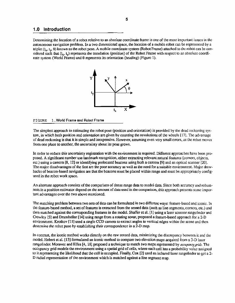
Determining the location of a robot relative to an absolute coordinate frame is one of the most important issucs in the autonomous navigation problem. In a two dimensional space, the location of a mobile robot can be represented by a triplet (L, t,, 0) known as the robot pose. A mobile coordinate system (Robot Frame) attached to the robot can be considered such that (&, ty) represents the translation @sition) of the Robot Frame with respect to an absolute coordinate system (World Frame) and e represents its orientatim (heading) (Figure 1).

FIGURE 1. World Frame and Robot Frame

The simplest apprmch in estimating the robot pose (position and orientation) is provided by the dead reckoning system, in which both position and orientation are given by counting the revolutions of the wheels I171. The advantage of dead reckoning is that it is simple and inexpensive. However, assuming even vely small errors, as h e robot moves from one place to another, the uncertainty about its pose grows.

In order to reduce this uncertainty regisuation with the environment is required. Different approaches have been proposed. A significant number use landmark recognition, either extracting relevant natural fcatures (corners, objects, etc.) using a camera [S. 121 or identifying plocated beacons using both a camera [91 and an optical scanner [201. The major disadvantages of the first are the p r accuracy as well as the need for a suitable environment Major draw- backs of beacon-based navigation are that the beacons must be placed within range and must be approprialcly config- ured in the robot work space.

An alternate approach consists of the comparison of dense range data to model data. Since both accuracy and robusl- ness in a position estimator depend on Ihe amount of data used in the comparison, this approach presents some important advantages over the two above mentioned.

The matching problem between two sets of data can be formulated in two different ways: feature-based and iconic. In the feature-based method, a set of features is extracted from the sensed data (such as line segments, comers, elc.) and then matched against the corresponding features in the model. SMer et al. [l] using a laser scanner rangefinder and Crowley [5 ] and Drumheller [14] using mnge. from a rotating sonar, proposed a featurebased approach for a 2-D environment. Krotkov [ill used a single CCD camera to extract angles to vertical edges within the scene and then determine the robot pose by establishing their correspondence in a 2-D map.

In contrast, the iconic method works directly on the raw sensed data, minimizing the discrepancy bciween i t and the model. Hebert et al. [131 formulated an iconic method to compare two elevation maps acquired Crom a 3-D lascr rangefinder. Moravec and Elfes [4,18] proposed a technique to match two maps represented by occupancy~. The occupancy grid models the environment using a spatial grid of cells. where each cell has a probability value assigncd to it representing the likelihood that the cell is occupied. Finally, Cox [21 used an infrared laser rangefinder to get a 2- D radial representation of the environment which is matched against a line segment map.

6

In this paper. we present a new iconic approach for estimating the pose of a mobile robot equipped with a radial laser rangefinder. Unlike prior approaches. our method can be used in environments with only a minimal amounl o€ slruc- ture. provided enough is present to disambiguate the robot's pose. Our map consists of a possibly large number of short line segments, perhaps constructed by the rangefinder itself, lo approximately represent any environment shapc. This representation introduces problems in map indexing and error minimization which are addressed to insure that accurate estimates can be computed quickly.

2.0 Problem statement

The position estimation problem consists of two parts: sensor to map data correspondence and error minimization. Correspondence is the task of determining which map data point gave rise to each sensor data point. Once the c o r n spondence is computed, error minimization is the task of computing a robot pose that minimizes the error (e.g.. distance) between the actual location of each map data point and the sensor's estimate of its location. In this section we formalize these two parts.

Let A be a set of sensed data points taken from a certain robot position, and B be a set of either sensed data extracted from a different position or a set of data describing a world map. The matching problem for posilion estimation can be stated as how to determine the best mapping of A onto B. in other words, how to compute the transformation T which minimizes an appropriate emx function:

E = O ( T ( A ) , B ) ( E Q 1)

Consider a world map M desnibed by a set of data M = (MI, Mz, ... ,Mm] expressed in an absolute coordinate system (World Frame) and sensed data S = (SI, Sz. ... .Sa], where Si is expressed in a local coordinate system attached to the mobile robot (Robot Frame). Then, the robot position estimation consists of solving the minimization problem:

min, E = O ( T ( S ) . M ) ( E Q 2 )

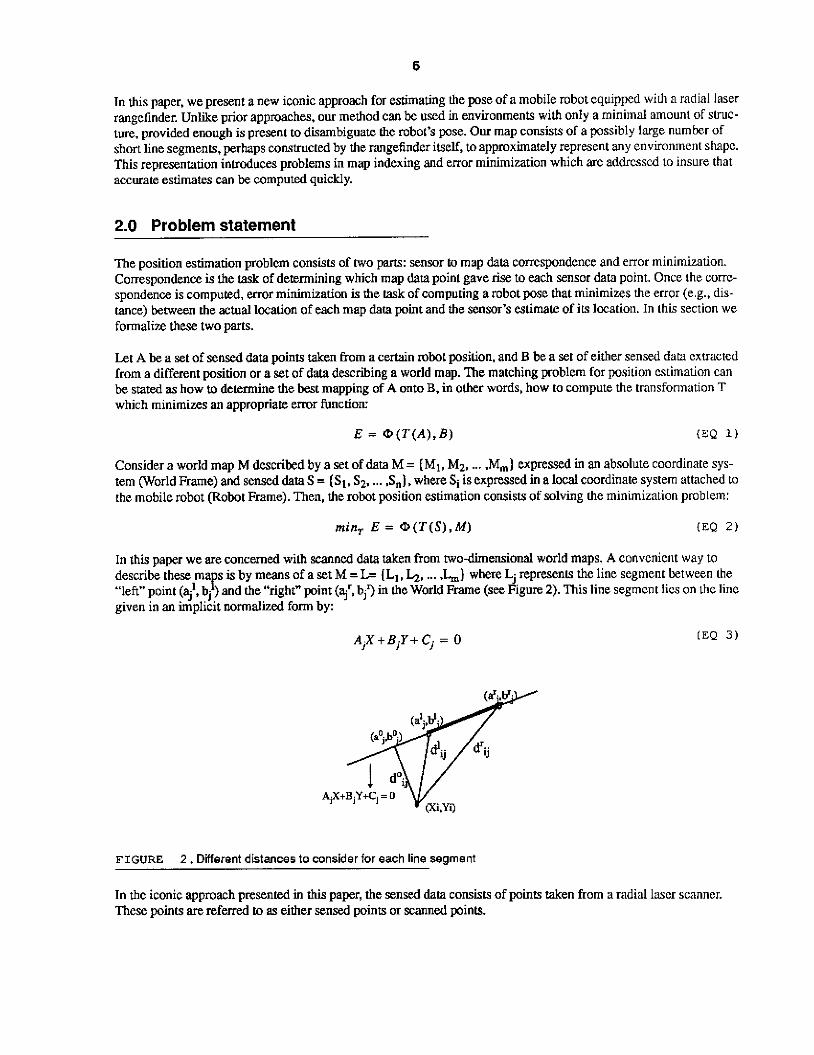
In this paper we are wncemed with scanned data taken from two-dimensional world maps. A convenient way M describe these. ma s is by means of a set M = L= (L1, b, ... &) where Lj represents the line segment between the

given in an implicit normalized form by: "left" point (5'. b. P )and the "right" point (9: bj3 in che World Frame (see Figure 2). This line segment lies on the line

J .

A,X+BjY+Cj = 0 IEQ 3)

FIGURE 2 . Different distances to consider for each line segment

In the iconic approach presented in this paper, the sensed data consists of points taken from a radial lascr scanner. These points are referred to as either s e d points or scanned points.

7

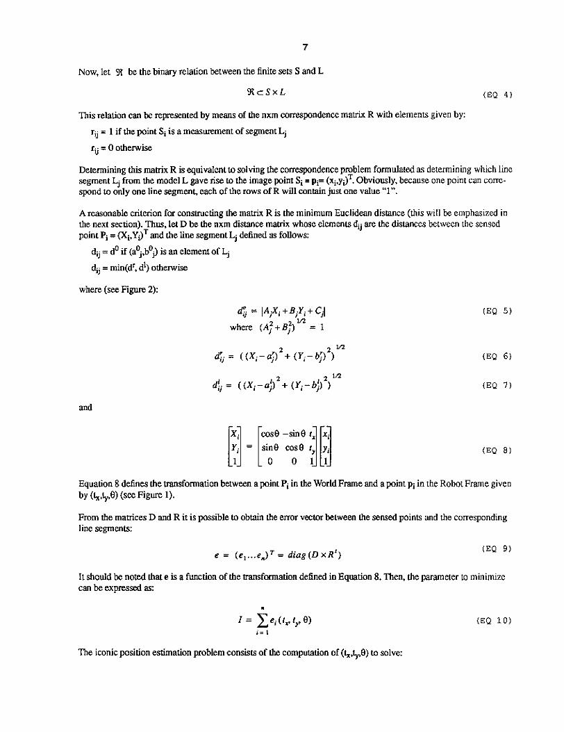
Now, let 3 be the binary relation between the finite sets S and L

S C S X L (EQ 4 )

This relation can be represented by means of the nxm cmrespondence matrix R with elements given by:

rij = 1 if the point Si is a measurement of segment Lj

rij = 0 otherwise

Determining this mahix R is equivalent to solving the correspondence problem formulated as determining which linc segment Lj from the model L gave rise to the image pint Si = pi= (xi.yijT. Obviously, because one point can corn- spond to only one line segment, each of the rows of R will contain just one value "1".

A reasonable criterion for constructing the matrix R is the minimum Euclidean distance (this will be emphasized in the next section). Thus. let D be the nxm distance matrix whose elements qj are the distances between the sensed point Pi = (Xi.YijT and the line segment Lj de6ned as follows:

dij = do if (aoj.boj) is an element of Lj 4- = min(dr, d') otherwise J

where (see Figure 2):

and

4j = IAjXi +BjY; + C;l

where (A;+B;) = 1 m

d! . = ((xi-=;) 2 + (Y,-b;) , 2 ) '* ,I

(EQ 5 )

Equation 8 defines the transformation between a point Pi in the World Frame and a point pi in the Robot Frame given by (t&$) (see Figure 1).

From the matrices D and R it is possible to obtain the error vector between the sensed points and the corresponding [me segments:

(EQ 9) e = (e, ... eJT = d i n g ( D x R ' )

It should be noted that e is a function of the transformation defined in Equation 8. Then, the parameter to minimizc can be expressed as:

i = 1

The iconic position estimation problem consisrs of the computation of (t&,0) to solve:

In practice. the mauix R is derived from D by:

F*= 1if4r ,<4jforaUj

r, = 0 otherwise

Moreover, R is a “dynamic m a ~ x ” in the sense that it is updated after each iteration of the optimization algorithm to solve Equation 11. A similar approach was used by Cox [21.

Although the approach presented here to compute R is deterministic, this formulation enables onc 10 ucat lhc correspondence problem in a probabilistic way. In this formulation, the el em en^ rij of the manix R would no longer be either 1 or 0 but would express the probability that the point Pi cco~esponds to the segment line Lj.

One of the main issues when solving the matching problem is the hi h cost involved in computing h e nxm mauix D. In Section 3 we present a more efficient approach to determine DxR avohng the entire computaLion of the mauix D.

k ”

3.0 Iconic Position Estirnatlon

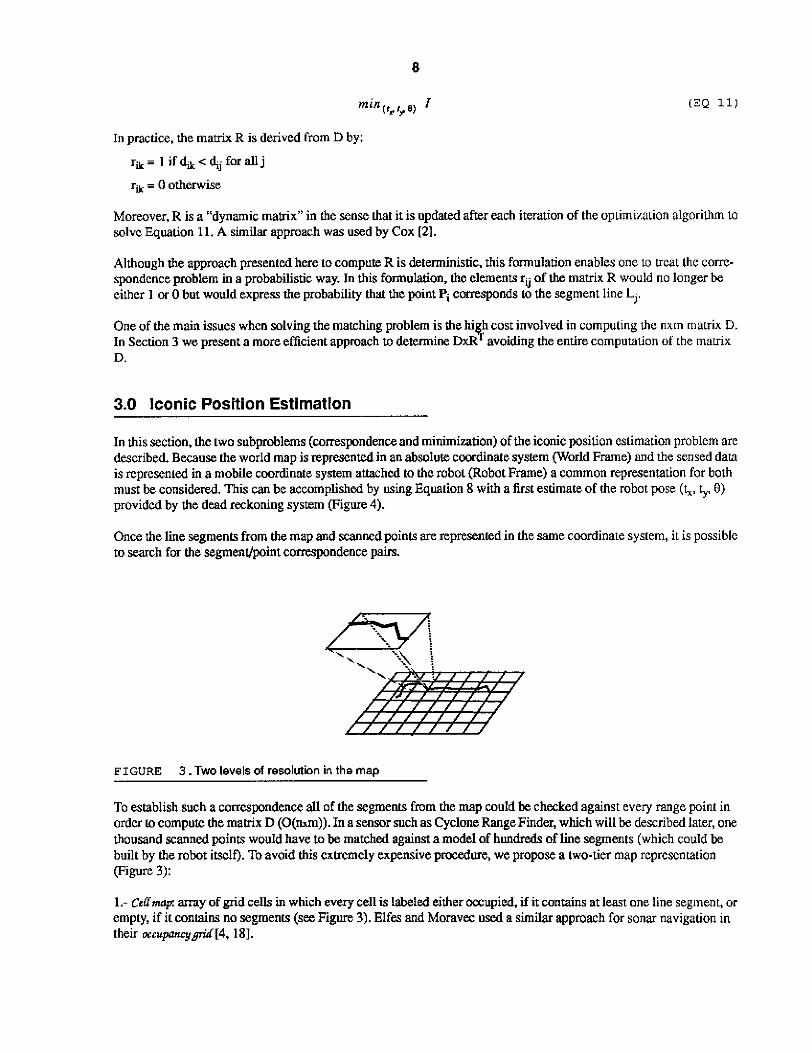
In this section. the two subproblems (correspondence and minimization) of the iconic position eslimation problem ore described. Because the world map is r e p e n t e d in an absolute coordinate system (World Frame) and the sensed data is represented in a mobile coordinate system attached to the robot (Robot Frame) a common representation for both must be considered. This can be accomplished by using Equation 8 with a first estimate of the robot pose (k, 5 8) provided by the dead reckoning system (Figure 4).

Once the lime segments from the map and scannedpoints are represented in the same coordinate system, it is possiblc to search for the segmenwint correspondence pairs.

FIGURE 3 .TWO levels of resolution in the map

To establish such a correspondence dl of the segments from the map could be. checked against every range point in order to compute the manix D (O(mm)). In a sensor such as Cyclone RangeFmder, which will be described later, one thousand scanned points would have to be matched against a model of hundreds of line segments (which could be built by the robot itselo. To avoid this extremely expensive procedure, we propose a two-tier map representation (Figure 3):

1.- Cellmap: array of grid cells in which every cell is labeled either occupied, if it contains at least one line segment, or empty, if it contains no segments (see Figure. 3). Elfa and Moravec used a similar approach for sonar navigation in their orcupatuy~[4,181.

9

2.-~ine m q collection of segments inside each of the occupied cells considered for correspondence.

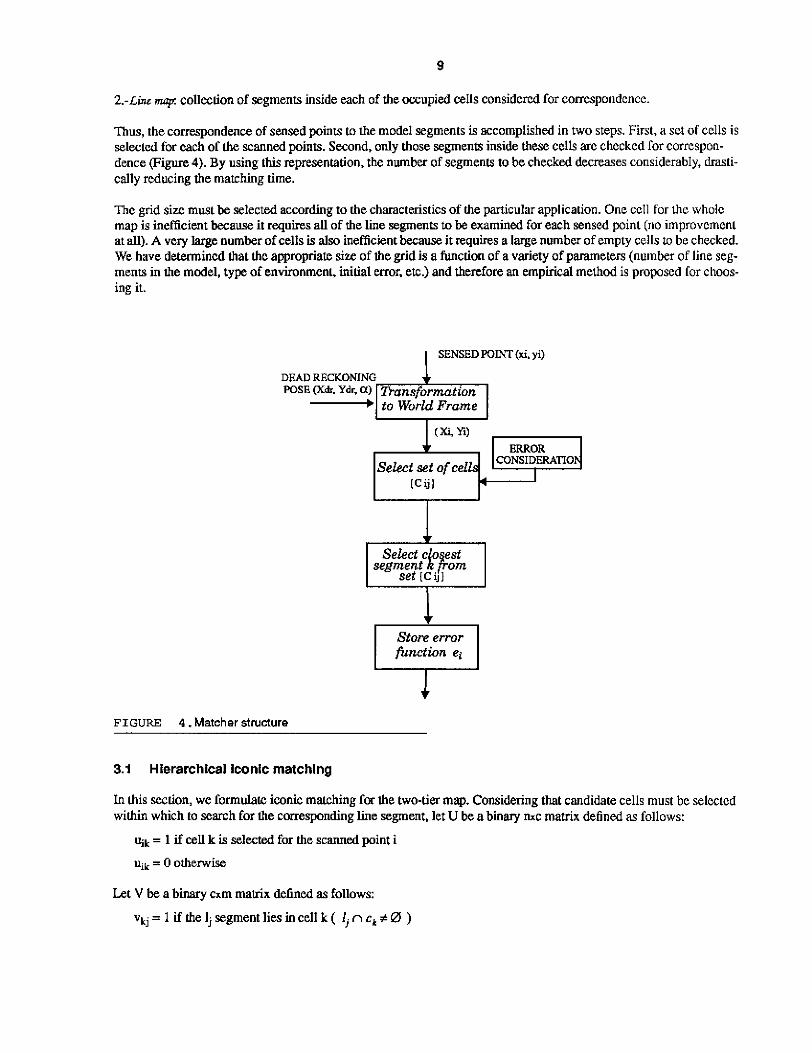
Thus, the correspondence of sensed points to the model segments is accomplished in two steps. First, a set of cells i s selected for each of the scanned points. Second, only those segments inside these cells are checked for correspondence ( F i i 4). By using this representation, the number of segments to be checked decreases considerably, dmsti- cally reducing the matching time.

The grid size must he selected according to the characteristics of the particular application. One ccll for the wholc map is inefficient because it requires all of the l i e segments to be examined for each sensed point (no improvement at all). A very large number of cells is also inef6cient because it requires a large number of empty cells to be checked. We have determined that the appropriate size of the grid is a function of a variety of parameters (number of line segments in the model. type of environment, initial mor. etc.) and therefore an empirical method is proposed for choos- ing it.

I SENSED POINT (xi, yi)

DEAD RECKONING

*- Select set of eel

function ei

+ FIGURE 4 . Matcher structure

3.1 Hierarchical iconic matching

In this section, we formulate iconic matching for the two-tier map. Considering that candidate cells must be selectcd within which to search for the corresponding line segment, let U be a binary llxc marrix defined as follows:

uik = 1 if cell k is selected for the scanned point i

Q = 0 otherwise

Let V be a binary cxm matrix defined as follows:

vk, = 1 if the lj segment lies incell k ( rjn ct #0 )

10

vkj = 0 otherwise

Consider the mm mahix W' given by the product UxV. The elements w'ij are given by:

k = l

Consider the mahix W defined as follows:

wij = 1 if w'- > 0 'J

w-.=Oifw'.--O 1J IJ -

Thus. a generic element wij from the matrix W indicates whether the segment 11 lies in any of the cells selected for the point Pi or not, and therefore if the distance between Ij and Pi must be computed or not.

For a given point Pi, assuming both U and V have been obtained, the number of distances to be computed reduces from m to m'i, where:

Although the matrix U must be calculated for each mmputed estimate, the matrix V is computed just once, when the map is built.

Notice that in the extreme case given above in which the number of cells considered for the ulmrrp (c) is very high (c >> in), the computation of matrix U (mc) could become more expensive that the straightforward approach of computing matrix D (O(mm)). In the following section the methodology to obtain the matrix U is presented.

3.2 Cell selection

After the scanned points have been transformed to the World Frame, a set of occupied cells must be selected for each of them (Figure 4). Due to mors in both dead reckoning and the sensor. in a significant number of cases, the points Pi are located in empty cells. We analyze these errors in more detail below.

3.2.1 Dead Reckonlng errors

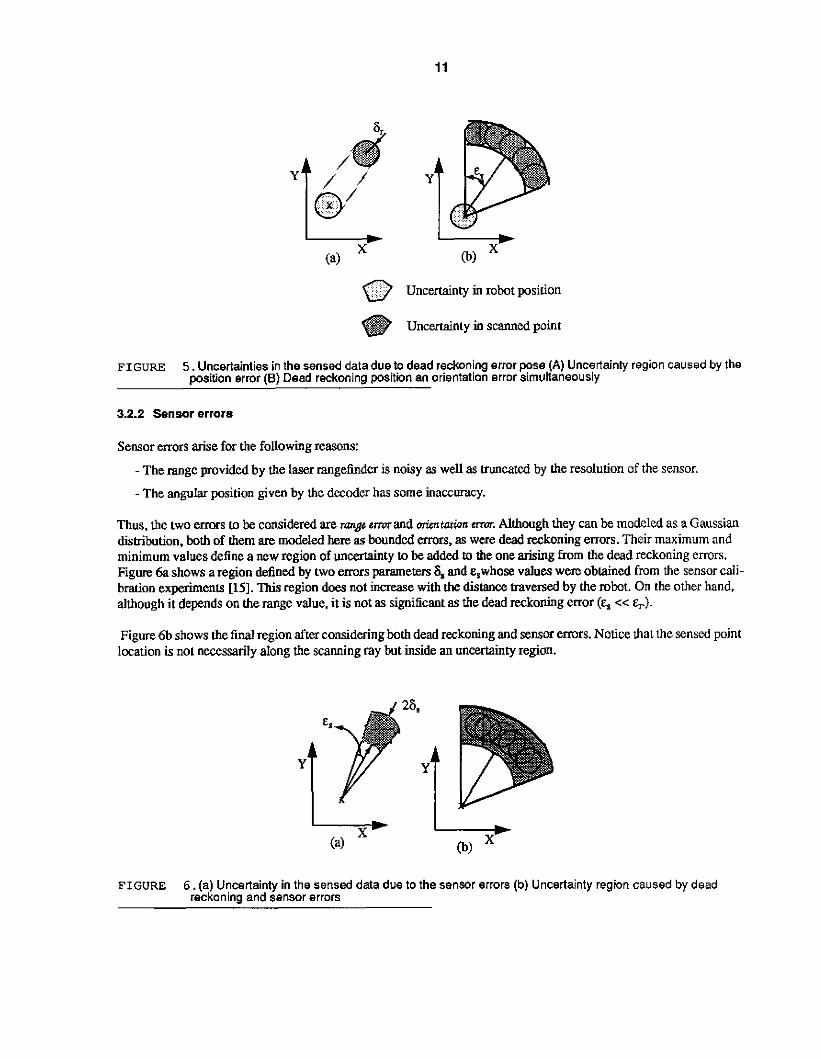
Dead reckoning is intrinsically vulnerable to bad calibration. imperfect wheel contact. upsetting events, etc. Thus, a bounded confidence region in which the actual location is likely to be found is used. This region is assumed to be a circle of radius S, proporbond to the traversed distance. This uncertainty in the robot position propagates in such a way that an identical uncertainty region centered at the sensed point can be considered (Figure 5a).

In a similar way, the heading error is assumed to be bounded by R, degrees. This error is also considend to be pro- portional to the traversed distance. Notice that the effect of this error over the uncertainty region depends on the range-the bigger the range the larger the uncertainty region (Figure 5b).

11

0 Uncertamty in robot position

Uncertainty in scanned point

FIGURE 5. Uncertainties in the sensed datadue to dead reckoning error pose (A) Uncertainty region caused by the position error (6) Dead reckoning p i t i o n an orientation error simultaneously

3.2.2 Sensor errors

Sensor errors arise for the following reasons:

- The range provided by the laser rangefinder is noisy as well as truncated by the resolution of the sensor.

- The angular position given by the decoder has some inaccuracy.

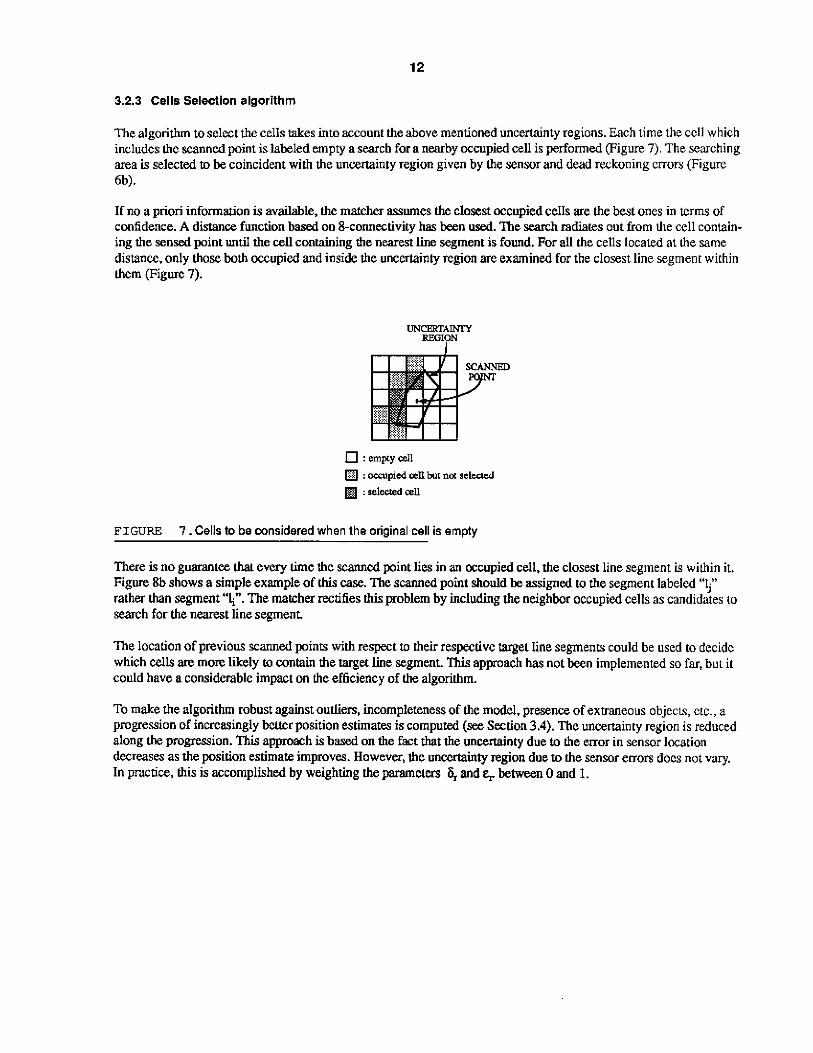
Thus, the two e m s to be considered are mngr rrmrand mientation m. Although they can be modeled as a Gaussian distribution, both of them are modeled here BS bounded m s , as were dead reckoning errors. Their maximum and minimum values define a new region of uncertainty to be added to the one arising from the dead reckoning errors. Figure 6a shows a region defined by two errors parameters S, and &,whose values were. obtained from the sensor cdi- bration experiment8 [15]. This region does not i n m e with the distance traversed by the robot. On the other hand, although it depends on the range value. it is not as significant as the dead redconhg error (Es << &I.

Figure 6b shows the final region after considering both dead reckoning and sensor errors. Notice that the sensed point location is not necessarily along the scanning ray but inside an uncertainty region.

FIGURE 6 . (a) Uncertainty in the sensed data due to the 9en5or errors (b) Uncertainty region caused by dead reckoning and sensor errors

12

3.2.3 Cells Selectlon algorithm

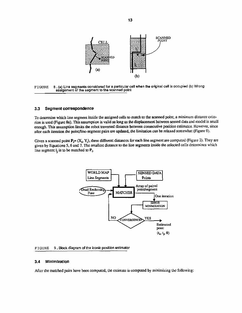
The algorithm to select the cells takes into account the above mentioned uncertainty regions. Each time the cell which includes the scanned point is labeled empty a search for a nearby occupied cell is performed (Figure 7). The searching area is selected m be coincident with the uncertainty region given by the sensor and dead reckoning errors (Figure a). If no a priori information is available, the matcher asrumes the closest occupied cells are the best ones in tcrms of confidence. A distance function based on &connectivity has been used. I h e seanh radiates out from the cell contain. ing the sensed point until the cell containing the nearest line segment is found. For all the cells located at the same distance, only those both occupied and inside the uncertainly region are examined for the closest line segment within them (Figure. 7).

FIGURE

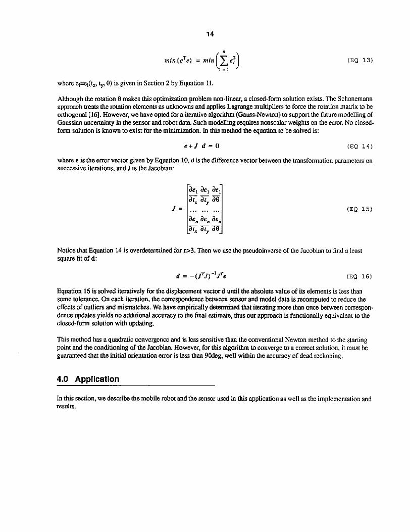
There is no guarantee that every time the scanned point lies in an occupied cell, the closest line segment is within it. Figure 8b shows a simple example of this case. The scanned point should be assigned to the segment labeled "$" rather than segment "4". The matcher rectifies this problem by including the neighbor occupied cells as candidates to search for the nearat line segment.

The location of previous scanned points with respect to their respective target line segments could be used to decide which cells are more likely to contain the target line segment. This approach has not been implemenred so far, but it could have a considerable impact on the efficiency of the algorithm.

To make the algorithm robust against outliers, incompleteness of the model. presence of extraneous objecu, cic., a progression of increasingly beuer position estimates is computed (see Section 3.4). The uncertainty region is reduced along the progresrion. This approach is based on the fact that the uncertainty due to the error in sensor lacation decreases as the position estimate improves. However, the uncertainty region due to the sensor errors does not vary. In practice, this is accomplished by weighting the parameters 6, and q between 0 and 1.

7 .Cells to be mnsidered when the original cell is empty

13

FIGURE 8 . (a) Line segments considered for a pan'c. ar cell when the orig nal cell is occ-pea (0) Wrong assignment 01 the segment to the scanned point

3.3 Segment correspondence

To determine which line segment inside the assigned cells to match to the scanned point, a minimum dislancc criterion is used (Figure Sa). This assumption is valid as long as the displacement between sensed data and model is small enough. This assumption limits the robot traversed & a c e between consecutive position estimates. However, since after each iteration the point/line-segment pairs are update& the limitation can be relaxed somewhat (Figure 9).

Given a scanned point Pi= (Xi, Yi), three different distances for each line segment are computed (Figure 2). They are given by Equations 5.6 and 7. The smallest distance to the line segments inside the selected cells determines which line segment I, is to be matched to Pi.

Estimated pose:

FIGURE 9. Bbck diagram of the iconic position estimator

3.4 Mlnlmlzatlon

After the matched pairs have been computed. the estimate is computed by minimizing the following:

rnin(eTe) = min Cei c:, (EQ 13)

where ei=q(&, $, (3) is given in Section 2 by Equation 11.

Although the rotation 0 makes this optimization problem non-linear, a closed-form solution exists. The Schonemann approach treats the rotation elements as unknow and applies Lagrange multipliers to force the rotation matrix to be orthogonal [ 161. However, we have opted for a iterative algorithm (Gauss-Newton) to support the future modelling of Gaussian uncertainly in the sensor and robot data Such modelling requires nonscalar weights on the error. No closed. form solution is hown to exist for the minimization. In this method the equation to be solved is:

e c I d = 0 (EQ 1 4 )

where e is the ermr vector given by Equation 10, d is the difference vector between the transformation parameters on successive iterations, and J is the Jacobian:

I = ... ... ... (EQ 1 5 )

Notice that Equation 14 is overdetermined for -3. Then we use the pseudoinverse of the Jacobian to find a least square fit of d:

LEQ 16) T -1 T d = - ( I J ) / e

Equation 16 is solved iteratively for the displacement vector d until the absolute value of its elements is less than some tolerance. On each iteration, the correspondence between se11s01 and model data is recomputed to reduce the effects of outliers and mismatches. We have empirically determined that iterating more than once between correspondence updates yields no additional accuracy to the final estimate, thus our approach is functionally equivalent io the closed-form solution with updating.

This method has a quadratic convergence and is less sensitive than the conventional Newton method lo the skuting point and the conditioning of the Jacobian. However, for this algorithm to converge to a c o m t solution, it must be guaranteed that the initial Orientation ermr is less than 90deg. well within the accuracy of dead reckoning.

4.0 Application

In this section, we describe the mobile robot and the sensor used in this application as well as the implementation and results.

15

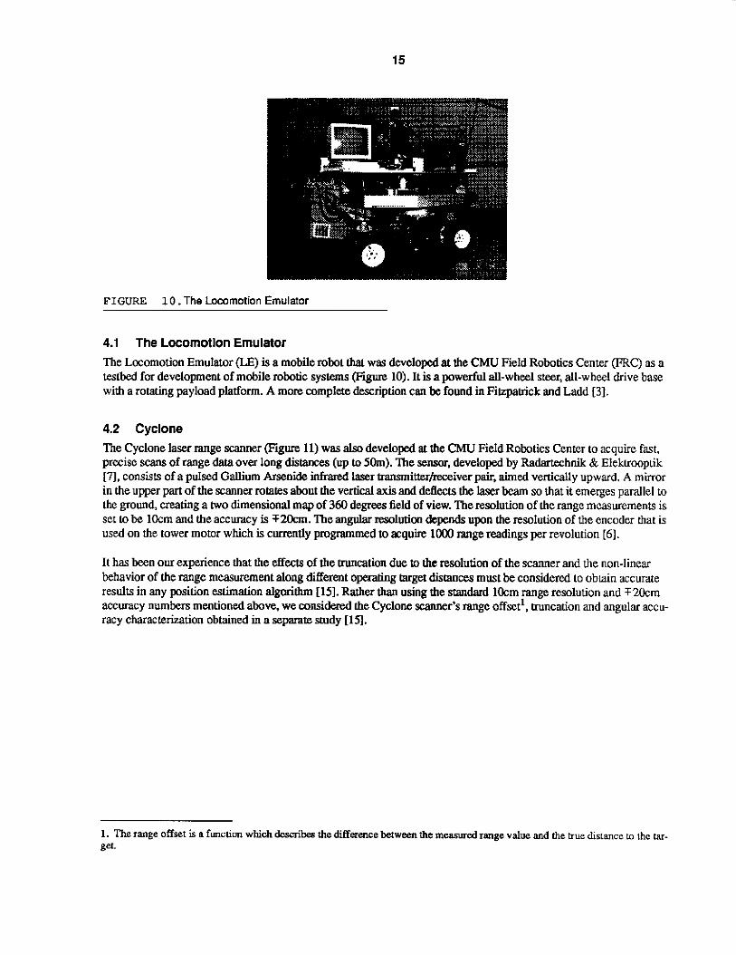
FIGURE 10 .The Locomotion Emulator

4.1 The Locomotion Emulator The Locomotion Emulator &E) is a mobile robot that was developed at the CMU Field Robotics Center as a testbed for development of mobile robotic systems (Figure IO). It is a powerful &-wheel steer, all-wheel drive base with a rotaring payload plalform. A more complete description can be found in Fiizpahick and Ladd [3].

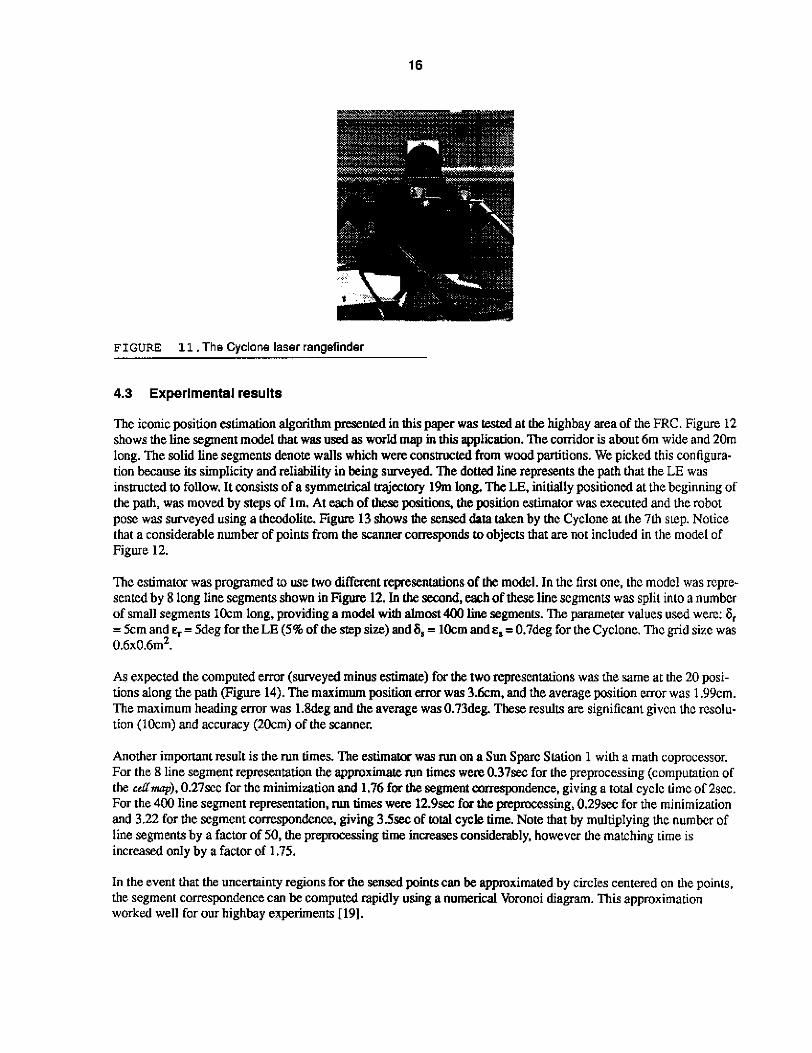
4.2 Cyclone The Cyclone laser range scanner (Figure 11) was also developed at the CMU Field Robotics Center to acquire fast, precise scans of range data o v a long distances (up to 5Om). The sensor, developed by Radamchnik & Elektrooptik [7]. consists of a pulsed Gallium Arsenide infrared laser transmitterbiver pair, aimed vertically upward. A mirror in the upper part of the scanner rotates about the vertical axis and ddects the l a w beam so that it emerges parallel to the ground, Creating a two dimensional map of 360 degrees field of view. Theresolution of the range measurements is set to be lOcm and the accuracy is TZOrm. The angular resoluticm depends upon the resolution of the encoder that is used on the tower rnomr which is currently programmed to acquire loo0 range. readings per revolution [6].

It has been our experience that the effects of the truncation due to the resolution of the scanner and the non-linear behavior of the range measurement along different operating distances must be considered to obtain accurate results in any position estimation algorithm [Is]. Rather than using the standard lOcm range resolution and T2Ocm accuracy numbers mentioned above, we consideaed the Cyclone scanner's range offset', mncation and angular accuracy characterization obtained in a separate study [la.

1. The range offset is a function which desnibes the difference between the m e m e 3 range value and the tme distance u1 Ihc target.

16

FIGURE 11 .The Cvclons laser ranaefinder

4.3 Experlrnental results

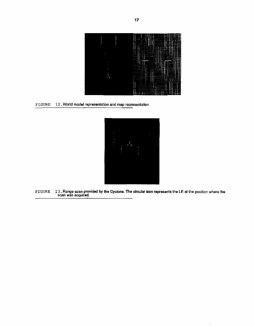
The iconic position estimation algorithm presented in h is paper was tested at the highbay area of the FRC. Figure 12 shows the line segment model that was used as world map m this a p p l i c h n . The conidor is a b u t 6 m wide and 2Om long. The solid line segments denote walls which were constructed from wood partitions. We picked this configura- tion because its simplicity and reliability in being surveyed. The dotted line represents the path that the LE was insmcted to follow. It consists of a symmeuical trajectory 1% long. The LE, initially positioned at the beginning of the path, was moved by steps of lrn. At each of these positiWs, the position estimator was executed and the robot pose was surveyed using a theodolite. Figure 13 shows the sensed data taken by the Cyclone at the 7th step. Notice that a considerable number of pints from the wamer cmresponds to objects that are not included in the model of Figure 12.

?he estimator was propmed to use two different representations of the model. In the first one, the model was represented by 8 long line segments shown in Figure 12. In the second, each of these line segments was split into a number of small segments lOcm long, providing a model with almost400 line segments. The parameter values used were: 6, = 5cm and &= Meg for the LE(58 of the step size) and& = lkrn and&,= 0.7deg forthe Cyclone. The grid sue w& 0.6x0.6mz.

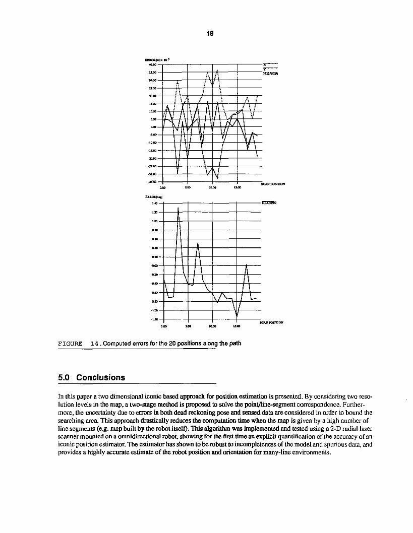
As expected the computed e m (surveyed minus estimate) for the two representations was the Same at the 20 positions along the path (Figure 14). The maximum position erro~ was 3.6cm. and the average p i t i o n error was 1.99cm. The maximum heading error was 1.8deg and the average was 0.73deg These results are significant given thc resolution (1Ckm) and accuracy (2orm) of the scanner.

Another important result is the run times. The estimatn wa m on a Sun Sparc Station 1 with a math coprocessor. For the 8 line segment representation the approximate run times wen?, 0 . 3 7 s for the preprocessing (compumtion of the cdmup) , 0 . 2 7 ~ for the minimization and 1.76 for the segment oorrespondence. giving a total cycle time of 2sec. For the 400 line segment representation, m times were 1 2 . 9 ~ for the preprocessing, 0 . 2 9 . ~ for the minimization and 3.22 for the segment correspondence. giving 3 . 5 ~ ~ of total cycle time. Note that by multiplying the number of line segments by a factor of 50, the preprocessing time increases considerably, however the matching time is increased only by a factor of 1.75.

In the event that the uncertainty regions for the &points can be appmximated by circles centered on the points, the segment correspondence can be computed rapidly using a numerical Vomnoi diagram. This approximation worked well for our highbay experiments [191.

17

FIGURE 12. World model representation and map representatin

FIGURE 13. Range scan provided by the Cycbne. The arcular icon represents the LE at the position where the scan was acauired.

18

FIGURE 14. Computed errors for the 20 positions along the path

5.0 Conclusions

In this paper a two dimensional iumic based approach for position estimation is presented. By considering two resolution levels in the map. a two-stage method is prop0tx.d m solve me point/linesegment correspondence. Further- more, the uncertainty due to errors in both dead teclroning pose and s m d data are considered in order to bound the searching ma This approach drastiEaUy reduces the computation time when the map is given by a high number of line segments (e.g. map built by the robot itself). ?his algorithm was implemented and tested using a 2-D radial laser Scanner mounted on a omnidirectional robot, showing fcf the 6rsl time an explicit quantilication of the accuracy of an iconic position estimator. The estimator has shown to berobust to incompleteness of the model and spurious data, and provides a highly accurate estimate of the robot position and orientation for many-line environments.

19

Future work includes the comparison of this method with a f e a m - W position estimation method by considering different memcs as accuracy. robusmess, starting point dependency, etc. and the development of a more complete navigation system including map building capability and a Gaussian uncertainty model for both the sensor and the robot motion.

Acknowledgements

We wish to thank to Gary Shaffer for his collaboration in the experiment and contribution to the development of the programs, Kerien Fitzpatrick for facilitating the testing, In So Kweon for suggesting the use of small line segments, and Sergio Sedas and Martial Hebert for their valuable comment!. and discussions.

References

[I] G. ShaFfer. A. Stentz, W. Whittaker, K. Fitzpatrick. ‘Tosition Estimator for Underground Mine Equipment”. In Proc. 10th WW International Mining Elecmtechnology Conference. Morgantown. W. VA, July 1990.

121 I. C. Cox. “Blanche-An Experiment in Guidance and Navigation of an Autonomous Robot Vehicle”. IEEE Trans- actions on Robotics and Automation, MI. 7. no. 2. April 1991.

[31 K. W. Fitzparrick and J.L. Law. “Locomotion Emulator: A testbed for navigation research”. In 1989 World Con- ference on Robotics Research The Next Five Years and Beyond, May 1989.

[41 H. P. Moravec and A. Elfes. ”High resolution maps from wide-angle sonar“. In Proc. IEEE International Confer- ence on Robotics Automation”, March 1985.

[51 J. L. Crowley. *‘Navigation for an intelligent mobilerobot”. IEEE Journal of Robotics and Automation, vol. RA-I, no. 1, March 1985.

[61 S. Singh, J. West, “Cyclone: A Laser Rangetinder for Mobile Robot Navigation”. Technical Report, CMU-RI-TR- 91 1991.

[7] -0, Laser-Rangefinder. Referenm Manual. RadarteChniCk&Elekuoopijlc, A-3754 Tabenreith 35, Austria.

[8] B. C. Bloom. W s e of landmarks for mobile robot navigation“. Io Proc. SPIE Conference on Intelligenl Robots and Computer Vision, vol. 579,1985.

[9] Z. L. Cao, JJ. Roning and E. L. Hall. “Omnidirectional vision navigation integrating beacon recognition with positioning”. In Proc. SPIE Conference on Intelligent Robots and Computer Vision, vol. 727, 1986.

[lo] M. P. Case. “Single landmark navigation by mobile robots“. In Proc. SPIE Conference on Intelligent Robots and Computer Vision. vol. 727,1986.

[I 11 E. Kmtkov. “Mobile robot localization using a single image”. In Roc. IEFZ Robotics and Aulomation Confer- ence. May 1989.

[121 H. P. Moravec. ”Robot Rover Viual Navigation”. Ann Arbor, MtUMI Research Press, 1981

[131 M. Hebert, T. Kanade. I. Kweon. “3-D Vision Techniques for Autonornous Vehicles”. Technical Report CMU- RI-TR-88-12. 1988.

t141 M. Dnunheller. “Mobile robot localization using sonar”. IEEE Tkansactions on Pattern Analysis and Machine Intelligence, vol. PAMI-9, no. 2, March 1987.

20

[Is] S. Sedas and J. Gonzalez. “Analytical and Experimental Characterization of a Radial Laser RangeFinder”.Tech- nicd Report CMU-RI-TR-91 1991.

[16] P. H. Schonemann and R. M. Carroll. “Fitting one matrix to another under choice of a central dilation and a rigid motion”, Psychomenika, vol. 35.p~. 245-255. June 1970.

[17] C. M. Wang, ‘location estimation and uncertainty analysis for mobile robots”, in Roc. IEEE Int. Conf. on Robotics and Automation, pp. 1230-1235,1988.

[18] A. Elfes. ‘5onar-basedreaLworld mapping and navigation”. IEEE Journal of Robotics and Automation, vol. RA-3, no. 3, June 1987.

[19] G. Shaffer and A. Stentz. “Automated Surveying of Mines Using a Scanning Laser Rangefinder”. IO be submit- ted to the SME Annual Meeting Symposium on Robotics and Automablon, February, 1993.

[201 C. D. MacGillem and T. S. Rappaport. “Infra-Red Location System for Navigation for Navigation of Autonomous Vehicles”. in Pnx. IEEE Int. Conf. on Robotics and Automation, pp. 12361238,1988.

An iconic position estimator for a 2D laser rangefinder

Documents