Sponsoring Committee: Professor Juan P. Bello, Chairperson Professor Yann LeCun Professor Panayotis Mavromatis AN EXPLORATION OF DEEP LEARNING IN CONTENT-BASED MUSIC INFORMATICS Eric J. Humphrey Program in Music Technology Department of Music and Performing Arts Professions Submitted in partial fulfillment of the requirements for the degree of Doctor of Philosophy in the Steinhardt School of Culture, Education, and Human Development New York University 2015

Welcome message from author
This document is posted to help you gain knowledge. Please leave a comment to let me know what you think about it! Share it to your friends and learn new things together.
Transcript
Sponsoring Committee: Professor Juan P. Bello, ChairpersonProfessor Yann LeCunProfessor Panayotis Mavromatis
AN EXPLORATION OF DEEP LEARNING IN CONTENT-BASED
MUSIC INFORMATICS
Eric J. Humphrey
Program in Music TechnologyDepartment of Music and Performing Arts Professions
Submitted in partial fulfillmentof the requirements for the degree of
Doctor of Philosophy in theSteinhardt School of Culture, Education, and Human Development
New York University2015

ACKNOWLEDGMENTS
There once was a time I thought it was some happy accident that I kept
finding myself in exactly the right place. Be it college, career, or concert, it
always felt like gravity, quietly inevitable, pulling me into the things I should
do, the places I should go, the opportunities I should pursue. But now, on
the backside of this arc, I can see quite plainly that I always had the direction
wrong; it was never a pull, but a push. Come to think of it, for as long as I
can seem to recall, I have been lucky enough to be surrounded by those who
would inspire, encourage, force, drag, and challenge me to always be better.
I am nothing short of blessed to be graced by the company and influence of
such wonderful human beings, and will try my best to thank as many of you
as I can here.
First and foremost, I am forever grateful to my grandparents —Glendolyn
& Norman, Elizabeth & Frank— for their myriad contributions, both concrete
and intangible. It is only for their love, diligence and sacrifice that any of
this is possible (but what I wouldn’t give to see your reactions now). This
goes doubly so for my parents, Sharon & Branden, who took a computer-
tinkering, dinosaur-building, saxophone-wielding dreamer and turned him into
a computer-sciencing, wood-working, guitar-wielding dreamer. Good job, guys.
An extra special thanks goes to my brothers, Steve & Tim, for all adventures,
past, present, and future, as we continue down the strangest of trails.
To those who had a most profound impact on my younger self: Paul
iii
Andersen, who helped introduce me to music, and more importantly, impro-
visation; Mary Bolton, who truly was “Mary E. Best”, and is near entirely to
thank (or blame) for my egregious use of analogy; Matt McGuire, who instilled
the virtues of hard work, effort, and discipline, and earned my deepest respect
for it; and Jayant Datta, who saw something in a kid with long hair and an
unhealthy love of delay pedals, and happily pushed him down the rabbit hole
of higher education.
To my professors and colleagues from my time in Miami for helping
me grow into a proper MuE. I cannot thank Corey Cheng and Colby Leider
enough, the former for his focused direction and the latter for the opposite. To
my classmates, you have influenced more than you know, both then and now:
without the positive influence of Chris Santoro I would be a different person
I am today; Estefania Cano, for setting the highest bars of scientific prowess,
musicality, and humility; Glen Deslauriers, who brought the creativity, heart,
and synths in spades; and to Patrick O’Keefe and Reid Draper, who helped
stoke the coals of ambition into a blaze.
To my friends and mentors —and those that are both— from NYU:
thanks to Aron Glennon, for conversations that always pushed the boundaries
of what either of us understood; to Areti Andreopoulou, Taemin Cho, Jon
Forsyth, whose experience and knowledge helped guide me through the deep,
dark forest of doctoral studies. thanks to Oriol Nieto and Braxton Boren,
without whom I cannot imagine getting this far, nor do I want to; to Finn
Upham, Michael Musick, Rachel Bittner, and Andrew Telichan, for your di-
verse perspectives, curious minds, and consistently sunny dispositions; and, to
Brian McFee and Justin Salamon, who even now continue to push me out into
deeper waters to swim alongside them.
iv

A special thanks to Ron Weiss, Ryan Rifkin, and Dick Lyon for the op-
portunity of a lifetime; working with you was as enjoyable as it was formative,
and I am forever in your debt.
Finally, a special thank you to my committee: to Panayotis Mavromatis,
whose expertise across various facets of music has been instrumental in the
course of my studies; to Yann LeCun, for sharing your wisdom and knowledge,
and showing me the ways of the Force; and to Juan Pablo Bello, for taking
me under his wing, being the perfect counterweight, and showing me how to
devine clarity from chaos. You have been a fantastic advisor and friend, and
I can only hope the things I’ve learned will generalize in the wild.
v
TABLE OF CONTENTS
LIST OF TABLES ix
LIST OF FIGURES xi
CHAPTER
I INTRODUCTION 1
1 Scope of this Study 52 Motivation 73 Dissertation Outline 94 Contributions 95 Associated Publications by the Author 10
5.1 Peer-Reviewed Articles 105.2 Peer-Reviewed Conference Papers 11
II CONTEXT 13
1 Reassessing Common Practice in Automatic Music Descrip-tion 161.1 A Concise Summary of Current Obstacles 22
2 Deep Learning: A Slightly Different Direction 232.1 Deep Architectures 242.2 Feature Learning 262.3 Previous Deep Learning Efforts in Music Informatics 30
3 Discussion 31
III DEEP LEARNING 33
1 A Brief History of Neural Networks 331.1 Origins (pre-1980) 341.2 Scientific Milestones (1980–2010) 391.3 Modern Rennaissance (post-2010) 45
2 Core Concepts 462.1 Modular Architectures 472.2 Automatic Learning 56
vi
2.3 Tricks of the Trade 623 Summary 69
IV TIMBRE SIMILARITY 70
1 Context 701.1 Psychoacoustics 711.2 Computational Modeling of Timbre 741.3 Motivation 761.4 Limitations 78
2 Learning Timbre Similarity 782.1 Time-Frequency Representation 802.2 Deep Convolutional Networks for Timbre Embedding 812.3 Pairwise Training 83
3 Methodology 863.1 Data 873.2 Margin Ratios 883.3 Comparison Algorithm 893.4 Experimental Results 91
4 Conclusions 102
V AUTOMATIC CHORD ESTIMATION 104
1 Context 1041.1 Musical Foundations 1051.2 What is a “chord”? 1091.3 Chord Syntax 1131.4 Motivation 1151.5 Limitations 117
2 Previous Research in Automatic Chord Estimation 1182.1 Problem Formulation 1182.2 Computational Approaches 1192.3 Evaluation Methodology 122
3 Pilot Study 1273.1 Experimental Setup 1273.2 Quantitative Results 1303.3 Qualitative Analysis 1313.4 Conclusions 137
4 Large Vocabulary Chord Estimation 1384.1 Data Considerations 1394.2 Experimental Setup 1424.3 Experimental Results 1504.4 Rock Corpus Analysis 161
vii
4.5 Conclusions & Future Work 1685 Summary 172
VI FROM MUSIC AUDIO TO GUITAR TABLATURE 174
1 Context 1752 Proposed System 178
2.1 Designing a Fretboard Model 1792.2 Guitar Chord Templates 1802.3 Decision Functions 182
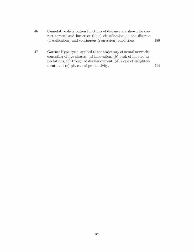
3 Experimental Method 1833.1 Training Strategy 1833.2 Quantitative Evaluation 184
4 Discussion 189
VII WORKFLOWS FOR REPRODUCIBLE RESEARCH 191
1 jams 1921.1 Core Design Principles 1941.2 The JAMS Schema 1961.3 Python API 197
2 biggie 1983 optimus 1994 mir_eval 2015 dl4mir 2036 Summary 203
VIII CONCLUSION 205
1 Summary 2052 Perspectives on Future Work 208
2.1 Architectural Design in Deep Learning 2082.2 Practical Advice for Fellow Practitioners 2112.3 Limitations, Served with a Side of Realism 2132.4 On the Apparent Rise of Glass Ceilings in Music
Informatics 216
BIBLIOGRAPHY 219
viii
LIST OF TABLES
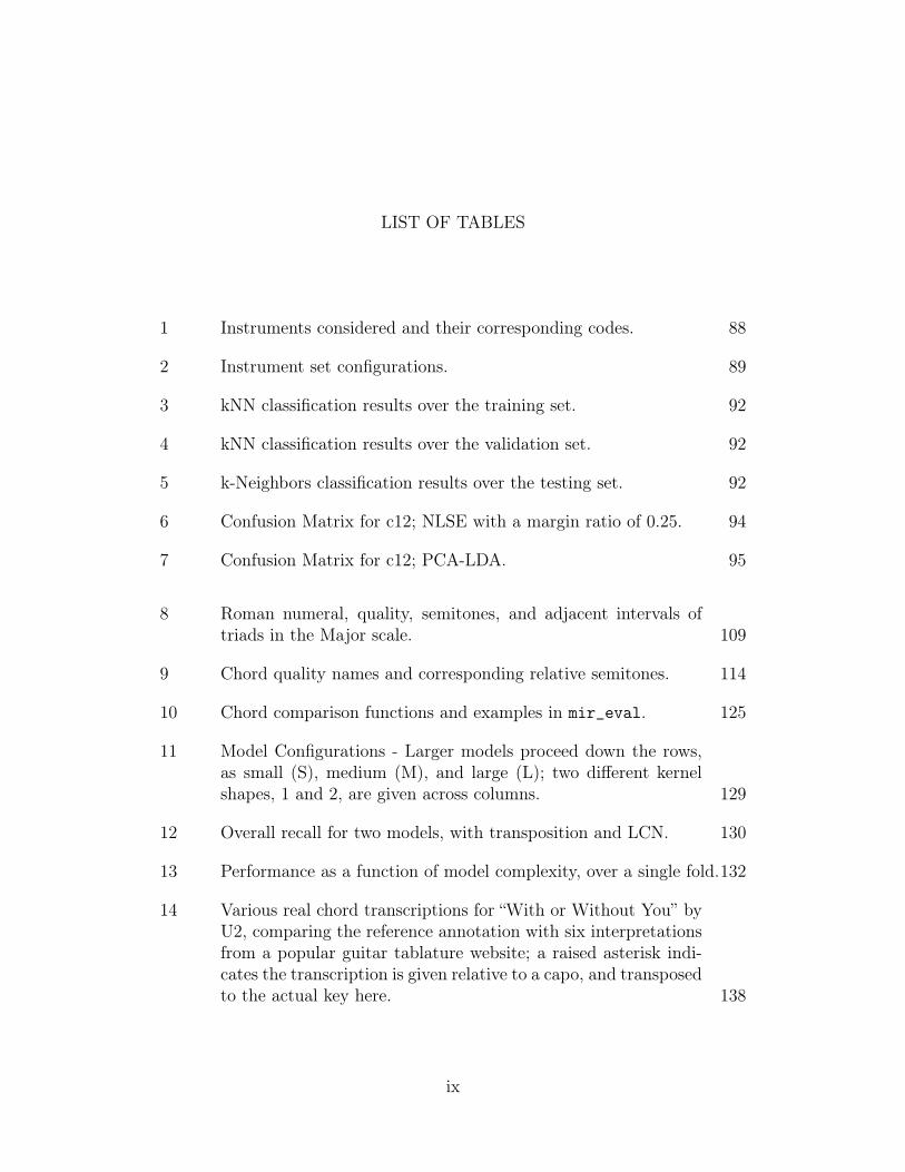
1 Instruments considered and their corresponding codes. 88
2 Instrument set configurations. 89
3 kNN classification results over the training set. 92
4 kNN classification results over the validation set. 92
5 k-Neighbors classification results over the testing set. 92
6 Confusion Matrix for c12; NLSE with a margin ratio of 0.25. 94
7 Confusion Matrix for c12; PCA-LDA. 95
8 Roman numeral, quality, semitones, and adjacent intervals oftriads in the Major scale. 109
9 Chord quality names and corresponding relative semitones. 114
10 Chord comparison functions and examples in mir_eval. 125
11 Model Configurations - Larger models proceed down the rows,as small (S), medium (M), and large (L); two different kernelshapes, 1 and 2, are given across columns. 129
12 Overall recall for two models, with transposition and LCN. 130
13 Performance as a function of model complexity, over a single fold.132
14 Various real chord transcriptions for “With or Without You” byU2, comparing the reference annotation with six interpretationsfrom a popular guitar tablature website; a raised asterisk indi-cates the transcription is given relative to a capo, and transposedto the actual key here. 138
ix
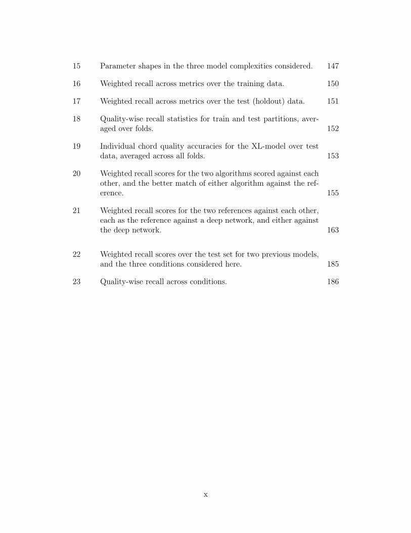
15 Parameter shapes in the three model complexities considered. 147
16 Weighted recall across metrics over the training data. 150
17 Weighted recall across metrics over the test (holdout) data. 151
18 Quality-wise recall statistics for train and test partitions, aver-aged over folds. 152
19 Individual chord quality accuracies for the XL-model over testdata, averaged across all folds. 153
20 Weighted recall scores for the two algorithms scored against eachother, and the better match of either algorithm against the ref-erence. 155
21 Weighted recall scores for the two references against each other,each as the reference against a deep network, and either againstthe deep network. 163
22 Weighted recall scores over the test set for two previous models,and the three conditions considered here. 185
23 Quality-wise recall across conditions. 186
x
LIST OF FIGURES
1 Losing Steam: The best performing systems at MIREX since2007 are plotted as a function of time for Chord Estimation (bluediamonds), Genre Recognition (red circles), and Mood Predic-tion (green triangles). 14
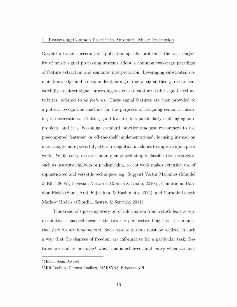
2 What story do your features tell? Sequences of MFCCs areshown for a real music excerpt (left), a time-shuffled versionof the same sequence (middle), and an arbitrarily generated se-quence of the same shape (right). All three representations haveequal mean and variance along the time axis, and could thereforebe modeled by the exact same distribution. 17
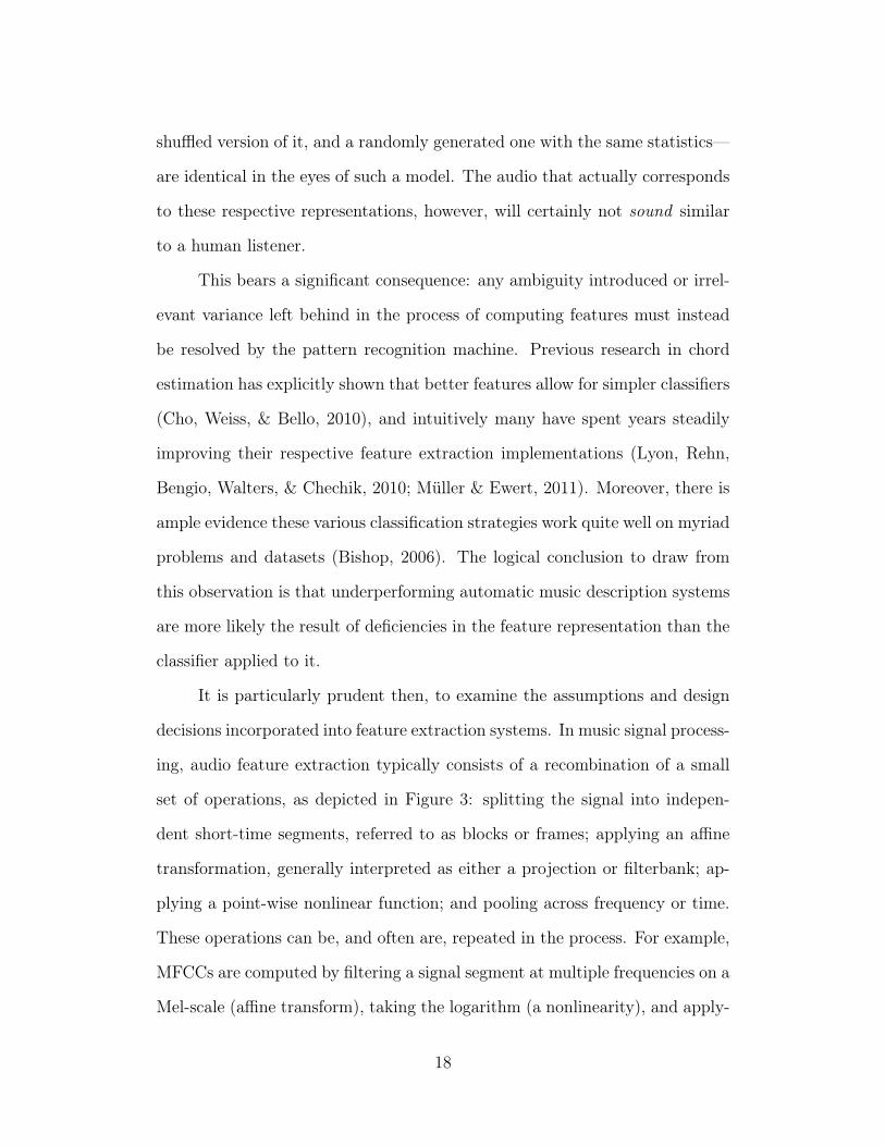
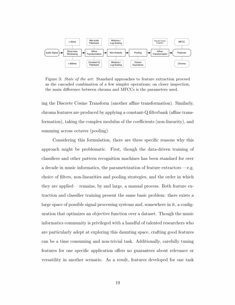
3 State of the art : Standard approaches to feature extraction pro-ceed as the cascaded combination of a few simpler operations;on closer inspection, the main difference between chroma andMFCCs is the parameters used. 19
4 Low-order approximations of highly non-linear data: The log-magnitude spectra of a violin signal (black) is characterized bya channel vocoder (blue) and cepstrum coefficients (green). Thelatter, being a higher-order function, is able to more accuratelydescribe the contour with the same number of coefficients. 21
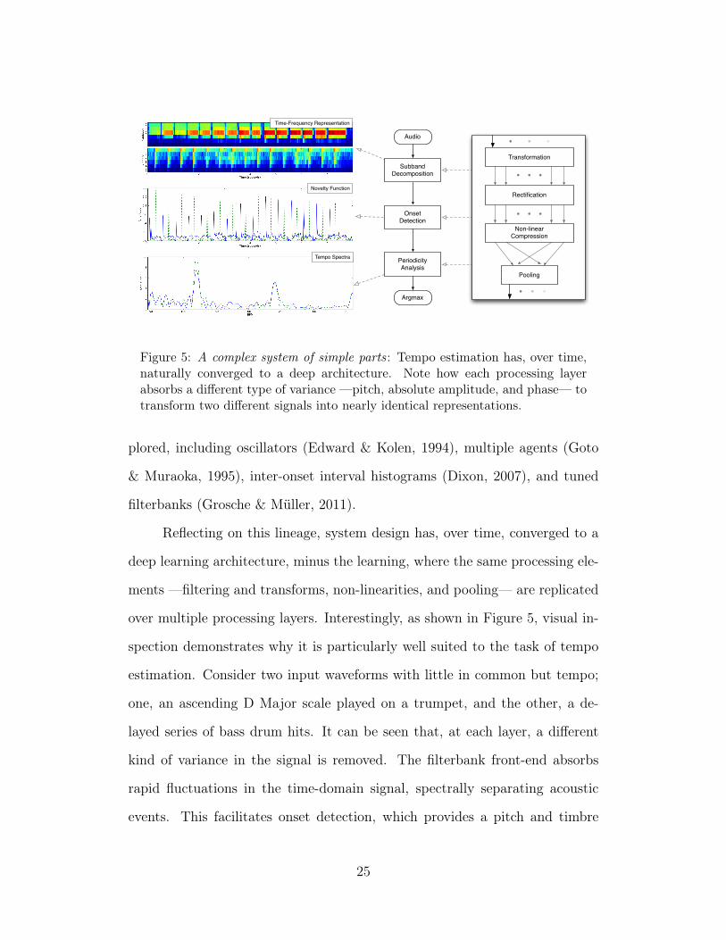
5 A complex system of simple parts : Tempo estimation has, overtime, naturally converged to a deep architecture. Note how eachprocessing layer absorbs a different type of variance —pitch, ab-solute amplitude, and phase— to transform two different signalsinto nearly identical representations. 25
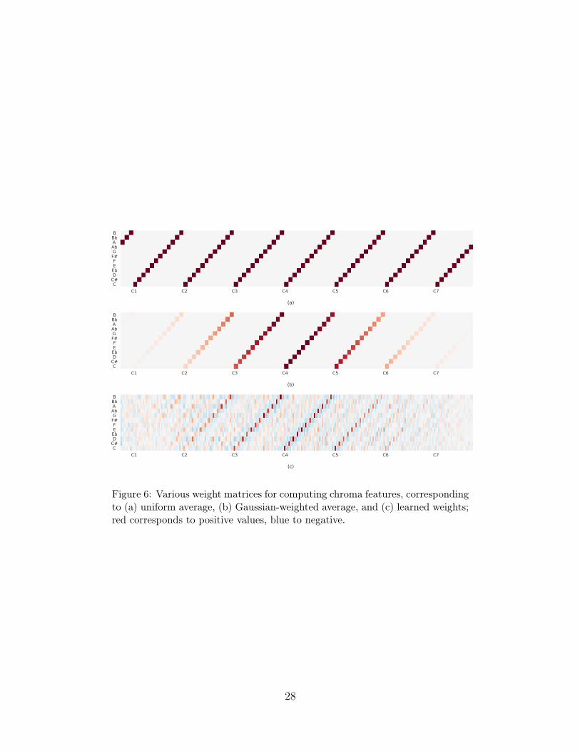
6 Various weight matrices for computing chroma features, corre-sponding to (a) uniform average, (b) Gaussian-weighted average,and (c) learned weights; red corresponds to positive values, blueto negative. 28
xi
7 Comparison of manually designed (top) versus learned (bottom)chroma features. 29
8 Linearly separable data classified by a trained perceptron. 37
9 Demonstration of the decision boundaries for a multi-layer per-ceptron. 39
10 Hill-climbing analogy of gradient descent. 60
11 The resulting MDS model developed in the work of Grey. 73
12 Screenshot of the Freesound homepage. Immediately visible areboth the semantic descriptors ascribed to a particular sound(left), and the primary search mechanism, a text field (right). 77
13 Diagram of the proposed system: a flexible neural network istrained in a pairwise manner to minimize the distance betweensimilar inputs, and the inverse of dissimilar ones. 80
14 Distribution of instrument samples in the Vienna SymphonicLibrary. 89
15 Loss contours for different margin ratios. 90
16 Embeddings of clarinet (blue circles), oboe (green diamonds),and cello (red squares) observations across models trained withthe “c5” instrument configurations. 96
17 Embeddings of clarinet (blue circles), oboe (green diamonds),and cello (red squares) observations across models trained withthe “c8” (top) and “c8” (bottom) instrument configurations. 97
18 Embeddings of clarinet (blue circles), oboe (green diamonds),and cello (red squares) observations across models trained withthe “c12” instrument configurations. 98
19 Embeddings of clarinet (blue circles), oboe (green diamonds),and cello (red squares) observations across models trained withthe “c24” instrument configurations. 99
20 Recall-Precision curves over the four instrument configurations. 100
xii
21 A stable F major chord played out over three time scales, asa true simultaneity, an arpeggiation, and four non-overlappingquarter notes. 111
22 A stable C major chord is embellished by passing non-chord tones.111
23 A sample harmonic analysis of a piano piece, performed as amusic theory exercise. 112
24 Block-diagram of the common building blocks in modern auto-matic chord estimation systems. 120
25 Accuracy differential between training and test as a function ofchord class, ordered along the x-axis from most to least commonin the dataset for As-Is (blue) and Transposed (green) conditions.132
26 Effects of transposition on classification accuracy as a functionexplicitly labeled Major-Minor chords (dark bars), versus otherchord types (lighter bars) that have been resolved to their nearestMajor-Minor equivalent, for training (blue) and test (green) inAs-Is (left) and Transposed (right) conditions. 133
27 Histograms of track-wise recall differential between As-Is andTransposed data conditions, for training (blue), validation (red)and test (green) datasets. 135
28 Histogram of chord qualities in the merged data collection. 141
29 The visible effects of octave-dependent LCN, before (left) andafter (right). 143
30 A Fully Convolutional Chord Estimation Architecture. 145
31 Track-wise agreement between algorithms versus the best matchbetween either algorithm and the ground truth data. 156
32 Reference and estimated chord sequences for a track in QuadrantI, where both algorithms agree with the reference. 158
33 Reference and estimated chord sequences for a track in Quad-rant II, the condition where algorithms disagree sharply, but oneagrees strongly with the reference. 159
xiii
34 Reference and estimated chord sequences for a track in Quad-rant III, the condition where neither algorithm agrees with thereference, nor each other. 160
35 Reference and estimated chord sequences for a track in QuadrantIV, the condition where both algorithms agree with each other,but neither agrees with the reference. 161
36 Track-wise agreement between annotators versus the best matchbetween either annotator and the best performing deep network. 164
37 Reference and estimated chord sequences for a track in QuadrantI, where the algorithm agrees with both annotators. 165
38 Reference and estimated chord sequences for a track in QuadrantII, the condition where the annotators disagree sharply, but oneagrees strongly with the algorithm. 166
39 Reference and estimated chord sequences for a track in Quad-rant III, the condition where neither annotator agrees with thealgorithm, nor each other. 167
40 Reference and estimated chord sequences for a track in QuadrantIV, the condition where both annotators agree with each other,but neither agrees with the algorithm. 168
41 A possible chord hierarchy for structured prediction of classes.Decisions blocks are rectangular, with the result of the previousnode shown in parentheses, the semantic meaning of the nodeis given before a colon, and the set of valid responses is pipe-separated. Stopping conditions are given as octagons. 170
42 A chord sequence (top), traditional staff notation (middle), andguitar tablature (bottom) of the same musical information, indecreasing levels of abstraction. 175
43 Visitor statistics for the tab website Ultimate Guitar, as of Jan-uary 2015. 177
44 Full diagram of the proposed network during training. 181
45 Understanding misclassification as quantization error, given atarget (top), estimation (middle), and nearest template (bottom).187
xiv
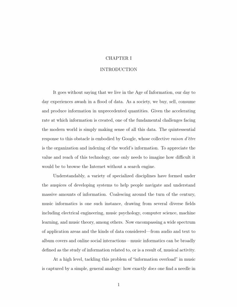
46 Cumulative distribution functions of distance are shown for cor-rect (green) and incorrect (blue) classification, in the discrete(classification) and continuous (regression) conditions. 188
47 Gartner Hype cycle, applied to the trajectory of neural networks,consisting of five phases: (a) innovation, (b) peak of inflated ex-pectations, (c) trough of disillusionment, (d) slope of enlighten-ment, and (e) plateau of productivity. 214
xv

xvi

“What’s it matter? Does it matter,If we’re all matter when we’re done,When the sky is full of zeros and ones?”
-Andrew Bird, Masterfade
xvii
CHAPTER I
INTRODUCTION
It goes without saying that we live in the Age of Information, our day to
day experiences awash in a flood of data. As a society, we buy, sell, consume
and produce information in unprecedented quantities. Given the accelerating
rate at which information is created, one of the fundamental challenges facing
the modern world is simply making sense of all this data. The quintessential
response to this obstacle is embodied by Google, whose collective raison d’être
is the organization and indexing of the world’s information. To appreciate the
value and reach of this technology, one only needs to imagine how difficult it
would be to browse the Internet without a search engine.
Understandably, a variety of specialized disciplines have formed under
the auspices of developing systems to help people navigate and understand
massive amounts of information. Coalescing around the turn of the century,
music informatics is one such instance, drawing from several diverse fields
including electrical engineering, music psychology, computer science, machine
learning, and music theory, among others. Now encompassing a wide spectrum
of application areas and the kinds of data considered—from audio and text to
album covers and online social interactions—music informatics can be broadly
defined as the study of information related to, or is a result of, musical activity.
At a high level, tackling this problem of “information overload” in music
is captured by a simple, general analogy: how exactly does one find a needle in
1
a haystack? To answer this question, any system, computational or otherwise,
must solve two related problems: first, it is necessary to describe the intrinsic
qualities of the item of interest, e.g. a needle is metal, sharp, thin, etc; and
second, it is necessary to evaluate the extrinsic relationships between items
to determine relevance. A piece of hay is certainly not a needle, for example,
but is a pin close enough? Along what criteria might we gauge similarity, or
classify objects into groups? Emphasizing the distinction, description focuses
on absolute representation, whereas comparison is concerned with relative as-
sociations.
To date, the most successful approaches to large-scale information sys-
tems leverage human-provided signals to achieve rich content descriptions.
Building on top of robust representations simplifies the problem greatly, and
good progress has been made toward the development of useful applications.
For example, the Netflix Prize challenge1 —an open contest to find the best
system for automatically predicting a user’s enjoyment of a movie— was built
exclusively on movie ratings contributed by a large collection of other users.
Similarly, Google’s PageRank algorithm associates websites based on how users
have linked different pages together, thus facilitating the process of traversing
the Internet (Page, Brin, Motwani, & Winograd, 1999).
While this strategy of leveraging manual content description has proven
successful in large-scale music recommendation, such as Pandora Radio2, its
application to more general music information problems is fundamentally lim-
ited, manifesting in three related ways. First, human-provided information
1http://www.netflixprize.com/2http://www.pandora.com/
2
commonly used in such systems —clicks, likes, listens or shares— are easily
captured from, or as a natural by-product of, a user’s listening to music. It
is one thing to obtain a “thumbs up” for a song; it is quite another to ask
that same user to provide a chord transcription of it. Second, manual music
description may require a high degree of expertise or effort to perform. The
average music listener is not truly capable of transcribing chords from a sound
recording, whether or not she possesses the time or willingness to attempt
it. Finally, even given the skill, motivation, and infrastructure to manually
describe music, this approach cannot scale to all music content, now or in the
future. The Music Genome Project1, for example, has resulted in the manual
annotation of some 1M commercial recordings, at a pace of 20-30 minutes per
track; the iTunes Music Store, however, now offers over 43M tracks world-
wide2. To illustrate how vast this discrepancy is, consider the following: even
assuming the lower bound of 20 minutes, it would still take one sad individ-
ual 1,600 years of non-stop annotation to close that gap. More importantly,
this only considers commercial music recordings, neglecting amateur or un-
published content from websites like YouTube3 or Soundcloud4, the addition
of which makes this goal even more insurmountable. Given the sheer impossi-
bility for humans to meaningfully describe all recorded music, now and in the
future, truly scalable music information systems will require good automatic
systems to perform this task.
Thus, the development of computational systems to describe music sig-
1https://www.pandora.com/about/mgp2According to http://www.apple.com/itunes/music/, accessed 20 April, 2015.3https://www.youtube.com/4https://soundcloud.com/
3
nals, a flavor of computer audition referred to as content-based music infor-
matics, is both a valuable and fascinating problem. In addition to facilitating
the search and retrieval of large music collections, automatic systems capable
of expert-level music description are invaluable to users who are unable to
perform the task themselves, e.g. music transcription. Notably, this problem
is also very much unsolved, and given an apparent deceleration of progress,
some in the field of music informatics have begun to question the efficacy of
traditional research methods. Simultaneously, in the related fields of com-
puter vision and automatic speech recognition, a branch of machine learning,
referred to as deep learning, has shown great performance in various domains,
toppling many long-standing benchmarks. On closer inspection, one recog-
nizes considerable conceptual overlap between deep learning and conventional
music signal processing systems, further encouraging this promising union.
Synthesizing these observations, this study explores deep learning as a
general approach to the design of computer audition systems for music de-
scription applications. More specifically, the proposed research method pro-
ceeds thusly: first, methods and trends in content-based music informatics
are reviewed in an effort to understand why progress in this domain may be
decellerating, and, in doing so, identify possible deficiencies in this method-
ology; standard approaches to music signal processing are then reformulated
in the language and concepts of deep learning, and subsequently applied to
classic music informatics problems; finally, the behavior of these deep learning
systems is deconstructed in order to illustrate the advantages and challenges
inherent to this paradigm.
4
1 Scope of this Study
This study explores the use of deep learning in the development of systems for
automatic music description. Consistent with the larger body of machine per-
ception research, the work presented here aims to computationally model the
relationship between stimuli and observations made by an intelligent agent. In
this case, “stimuli” are digital signals representing acoustic waves, e.g. sound,
“observations” are semantic descriptions in a particular namespace, e.g. tim-
bre or harmony, and the agent being modeled is an intelligent human, e.g. an
expert music listener. In practice, the namespace of descriptions considered is
constrained to a particular task or application, such as instrument recognition
or chord estimation.
Furthermore, if the relationship between stimuli and observation is not
a function of the agent, this mapping is said to be “objective”. Objective rela-
tionships are those that are true absolutely by definition, such as the statement
“A C Major triad consists of the pitches C, E, and G.” Elaborating, all suffi-
ciently capable agents should always produce the same output given the same
input. Discrepancies between observations of the same stimuli are understood
as one or more of these perspectives being erroneous, resulting from either
simple error, bias, or a deficiency of knowledge. For objective relationships,
the quality of a model is determined by how often it is able to produce “right”
answers, often referred to as “ground truth”, to the questions being asked.
Conversely, input-output relationships that are a meaningful function of
the agent are said to be “subjective”. In contrast to the objective case, which
is fundamentally concerned with facts, a subjective observation is ultimately
an opinion. As such, an opinion can only be true or false insofar as it is
5
held by a competent agent. This is embodied, for example, in the statement
“That sounds like a saxophone.” Whether or not the stimuli originated from
a saxophone is actually irrelevant; a rational agent has made the observation,
and thus it is in some sense valid. Assessing the quality of a computational
model at a subjective task must therefore take one of two slightly different
formulations. The first transforms a subjective problem to an objective one
by considering the perspective of single agent as truth, and thus the quality
of a model is a function of how well it can mimic the behavior of that one
agent. Alternatively, the other approach attempts to determine whether or
not a model makes observations on par with other competent agents. In this
view, a computational system’s capacity to perform some intelligent task is
measured by its ability to convince humans that it is competent (or not) in
human ways, e.g. the Turing test (Turing, 1950).
The notions of, and inherent conflict between, objectivity and subjectiv-
ity in audition and music perception are central to the challenge posed by the
computational modeling of it. Arguably most facets of music perception are
subjective and vary in degree from task to task. However, while subjective
evaluation might be better suited toward measuring the quality or usability
of some computational system, the human involvement required by such as-
sessments make them prohibitively costly in both time and money to conduct
with any regularity. As a result, conventional research methodology in engi-
neering and computer science greatly prefers quantitative evaluation as a proxy
to qualitative responses collected from human subjects. Typically quantitative
methods proceed by collecting some number of input-output pairs from one or
more human subjects beforehand, and treating this data sample as objective
6
truth. Thus, regardless of whether or not a given task is indeed objective, it
is a significant simplification in methodology to treat it as one.
This is all to say that the validity and quality of a music description
is often determined by an objective fitness measure, not necessarily out of
correctness but rather tractability. Therefore, any quantitative measure is
only valid insofar as the assumption of objectivity is as well.
2 Motivation
The proposed research is primarily motivated by two complementary observa-
tions: one, large scale music signal processing systems are becoming necessary
to help humans navigate and make sense of an ever-increasing volume of mu-
sic information; two —and, more notably, the specific problem this work seeks
to address— the conventional research tradition in content-based music infor-
mation retrieval is yielding diminishing returns, despite many research areas
remaining unsolved.
In the most immediate sense, the proposed research will develop systems
to tackle various applications in music informatics. This will at least serve to
explore an alternative approach to conventional problems in the field. Based
on preliminary results, there is good reason to believe that deep learning may
in fact push the state of the art in some, if not most, applications in automatic
music description. Sufficiently advanced systems could be deployed in end-user
applications, such as navigating music libraries or computer-aided composition
and performance.
A thorough exploration and successful extension of deep learning to mu-
sic signal processing has the potential to encourage a broader study of these
7
methods. The impacts of such a development could be far reaching, but there
are two of particular note. First and foremost, drawing attention to a promis-
ing, but otherwise uncharted, research area opens new opportunities for fresh
ideas and perspectives. Additionally, deep learning automatically optimizes a
system to the data on hand, accelerating research and simplifying the overall
design problem. Therefore these methods yield flexible systems that can easily
adapt to new data as well as new problems, allowing researchers to seek out
novel, exciting applications.
Beyond the scope of music informatics, deep learning research in the
context of a different domain, with its own unique challenges, is likely to
produce discoveries beneficial to the broad audience of computer science and
information processing. One such area where this is likely to occur is in the
handling of time-domain signals and sequences. Computer vision, the field
in which most breakthroughs in deep learning have occurred, has invested
considerable effort in the study of static, 2D images. Certainly some have
extended these techniques to image sequences and video, but this is far more
the exception than the rule. Other sequential data, such as natural language,
in the form of text, speech signals, and motion capture data have also seen a
deal of study in deep learning circles. The tradition of music signal processing
draws heavily from digital signal theory, a field of study with a considerable
focus on an analytical understanding of time.
Therefore, this work offers several potential contributions, both theoret-
ical and practical, to a diverse audience, spanning users of technology, music
informatics, and the deep learning community on the whole.
8
3 Dissertation Outline
Chapter II reviews the current state of affairs in music informatics research,
providing context for this work.
Chapter III surveys the body of literature in deep learning, outlining core
concepts and definitions.
Chapter IV explores the application of deep learning toward the development
of objective timbre similarity spaces.
Chapter V considers the application of deep learning toward automatic chord
estimation, as a means to both improve the state of the art and better
understand the task at hand.
Chapter VI extends this chord estimation efforts to directly estimate human-
readable representations in the form of guitar tablature.
Chapter VII documents the software contributions resulting from this study,
contributing to the greater cause of reproducible research efforts.
Chapter VIII concludes this thesis, summarizing the work presented and of-
fering perspectives for future work and outstanding challenges.
4 Contributions
The primary contributions of this dissertation are listed below:
• Demonstrates an objective approach to the development of tim-bre similarity embeddings. The proposed approach extends previousefforts in using pairwise training of deep architectures by relaxing con-straints on the output space and generalizing the use of margins as a
9
ratio, rather than an absolute parameter; in addition to realizing a farmore discriminative instrument embedding than a shallow comparisonsystem overall, the margin ratio improves performance slightly over theoriginal pairwise training approach.
• Advances the state of the art in large vocabulary automaticchord estimation, while illustrating methodological limitationsin the current formulation of the task. Comprehensive error analy-sis is performed both by comparing two state of the systems against thereference chord transcriptions, as well as the proposed system againstanother dataset with multiple annotators. The insight gleaned from thisstudy is used to offer perspective on future directions for the task atlarge.
• Leveraged traditional chord transcriptions to develop an auto-matic guitar chord estimation system, which directly maps mu-sic audio to fingerings on a fretboard. Not only does this approachimprove some measures over the other large-vocabulary chord estimationsystem presented here, but it provides a user-friendly interface for bothlearning and soliciting feedback on system errors.
• Contributes, in whole or part, to several open source projectsto facilitate future efforts. In addition to a suite of tools that mayhelp serve the larger research community, this includes a framework toreproduce the experimental results and analysis contained herein.
5 Associated Publications by the Author
This thesis covers much of the work presented in the publications listed below:
5.1 Peer-Reviewed Articles
• Humphrey, E. J., Bello, J. P., and LeCun, Y. (2013) “Feature learningand deep architectures: new directions for music informatics.”Journal ofIntelligent Information Systems. 41 (3), 461–481.
10
5.2 Peer-Reviewed Conference Papers
• Humphrey, E. J., Salamon, J. Nieto, O., Forsyth, J., Bittner, R. M., andBello, J. P. “JAMS: A JSON Annotated Music Specification for Repro-ducible MIR Research.”Proceedings of the 15th International Society ofMusic Information Retrieval (ISMIR), Taipei, Taiwan, October 2014.
• Raffel, C., McFee, B., Humphrey, E. J., Salamon, J. Nieto, O., Liang,D., and Ellis, D. P. W. “mir eval: A Transparent Implementation ofCommon MIR Metrics”Proceedings of the 15th International Society ofMusic Information Retrieval (ISMIR), Taipei, Taiwan, October 2014.
• Humphrey, E. J. and Bello, J.P. “From Music Audio to Guitar Tablature:Teaching Deep Convolutional Networks to Play Guitar.” Proceedings ofthe International Conference on Acoustic Signals and Speech Processing(ICASSP), Florence, Italy, May 2014.
• Humphrey, E. J., Nieto, O., and Bello, J. P. “Data Driven and Discrim-inative Projections for Large Scale Cover Song Identification.”to appearin Proceedings of the 14th International Society of Music InformationRetrieval (ISMIR), Curitiba, Brazil, November 2013.
• Humphrey, E. J., Nieto, O., and Bello, J. P. “Data Driven and Discrimi-native Projections for Large Scale Cover Song Identification.”to appear inProceedings of the International Society of Music Information Retrieval(ISMIR), Curitiba, Brazil, November 2013.
• Humphrey, E. J. and Bello, J.P., “Rethinking Automatic Chord Recog-nition with Convolutional Neural Networks.” Proceedings of the Inter-national Conference on Machine Learning and Applications (ICMLA),Boca Raton, FL, December 2012.
• Humphrey, E. J., Bello, J. P., and LeCun, Y. “Moving Beyond FeatureDesign: Deep Architectures and Automatic Feature Learning in MusicInformatics.” Proceedings of the International Society of Music Informa-tion Retrieval (ISMIR), Porto, Portugal, October 2012.
11
• Nieto, O., Humphrey, E. J., and Bello, J. P. “Compressing Music Record-ings into Audio Summaries.”in Proceedings of the International Societyof Music Information Retrieval (ISMIR), Porto, Portugal, October 2012.
• Humphrey, E. J., Cho, T. and Bello, J.P. “Learning a Robust Tonnetz-space Transform for Automatic Chord Recognition.” Proceedings ofthe International Conference on Acoustic Signals and Speech Processing(ICASSP), Kyoto, Japan, March 2012.
• Humphrey, E. J., Glennon, A. and Bello, J.P., “Non-Linear Semantic Em-bedding for Organizing Large Instrument Sample Libraries.” Proceedingsof the International Conference on Machine Learning and Applications(ICMLA), Honolulu, HI, December 2011.
12
CHAPTER II
CONTEXT
From its inception, many fundamental challenges in music informatics,
and in particular those that focus on music audio signals, have received a
considerable and sustained research effort from the community. Referred to
here as automatic music description, this area of study is based on the premise
that if a human expert can experience or observe some musical event from an
audio signal, it should be possible to make a machine respond similarly. As the
field of music informatics continues into its second decade, there are a growing
number of resources that comprehensively review the state of the art in music
signal processing across a variety of different application areas (A. Klapuri &
Davy, 2006; Casey, Veltkamp, et al., 2008; Müller, Ellis, Klapuri, & Richard,
2011), including melody extraction, chord estimation, beat tracking, tempo
estimation, instrument identification, music similarity, genre classification, and
mood prediction, to name only a handful of the most prominent topics.
After years of diligent effort however, many well-worn problems in content-
based music informatics lack satisfactory solutions and remain unsolved. Ob-
serving this larger research trajectory at a distance, it would seem progress is
decelerating, if not altogether stalled. For example, a review of recent MIREX∗
results motivates the conclusion quantitatively, as shown in Figure 1. The
∗Music Information Retrieval Evaluation eXchange (MIREX): http://www.music-ir.org/mirex/
13
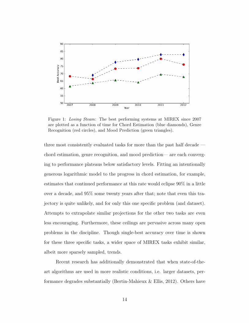
Figure 1: Losing Steam: The best performing systems at MIREX since 2007are plotted as a function of time for Chord Estimation (blue diamonds), GenreRecognition (red circles), and Mood Prediction (green triangles).
three most consistently evaluated tasks for more than the past half decade —
chord estimation, genre recognition, and mood prediction— are each converg-
ing to performance plateaus below satisfactory levels. Fitting an intentionally
generous logarithmic model to the progress in chord estimation, for example,
estimates that continued performance at this rate would eclipse 90% in a little
over a decade, and 95% some twenty years after that; note that even this tra-
jectory is quite unlikely, and for only this one specific problem (and dataset).
Attempts to extrapolate similar projections for the other two tasks are even
less encouraging. Furthermore, these ceilings are pervasive across many open
problems in the discipline. Though single-best accuracy over time is shown
for these three specific tasks, a wider space of MIREX tasks exhibit similar,
albeit more sparsely sampled, trends.
Recent research has additionally demonstrated that when state-of-the-
art algorithms are used in more realistic conditions, i.e. larger datasets, per-
formance degrades substantially (Bertin-Mahieux & Ellis, 2012). Others have
14
gone as far as to challenge the very notion that any progress has been made at
all, due to issues of problem formulation and validity (Sturm, 2014b). While
the truth of the matter likely falls somewhere between “erroneous results” and
“sound science”, these varied observations encourage a critical reassessment
of content-based music informatics. Does content really matter, especially
when human-provided information has proven to be more useful than rep-
resentations derived from the content itself (Slaney, 2011)? If so, what can
be learned by analyzing recent approaches to content-based analysis (Flexer,
Schnitzer, & Schlueter, 2012)? Do applications in content-based music infor-
matics lack adequate formalization and rigorous validation (Sturm & Collins,
2014)? Is the community considering all possible approaches to solve these
problems (Humphrey, Bello, & LeCun, 2012)?
Building on the premise that automatic music description is indeed valu-
able, this chapter is an attempt to answer the remainder of these questions.
Section 1 critically reviews conventional approaches to content-based analysis
and identifies three major deficiencies of current systems: the sub-optimality
of hand-designing features, the limitations of shallow architectures, and the
short temporal scope of conventional signal processing. Section 2 then intro-
duces the ideas of deep architectures and feature learning in terms of music
signal processing, two complementary approaches to system design that may
alleviate these issues, and surveys the application of these methods in this
domain. Finally, Section 3 summarizes the concepts covered herein, and dis-
cusses why it is critical point in time for the music informatics community to
consider alternative approaches.
15
1 Reassessing Common Practice in Automatic Music Description
Despite a broad spectrum of application-specific problems, the vast major-
ity of music signal processing systems adopt a common two-stage paradigm
of feature extraction and semantic interpretation. Leveraging substantial do-
main knowledge and a deep understanding of digital signal theory, researchers
carefully architect signal processing systems to capture useful signal-level at-
tributes, referred to as features. These signal features are then provided to
a pattern recognition machine for the purposes of assigning semantic mean-
ing to observations. Crafting good features is a particularly challenging sub-
problem, and it is becoming standard practice amongst researchers to use
precomputed features∗ or off-the-shelf implementations†, focusing instead on
increasingly more powerful pattern recognition machines to improve upon prior
work. While early research mainly employed simple classification strategies,
such as nearest-neighbors or peak-picking, recent work makes extensive use of
sophisticated and versatile techniques, e.g. Support Vector Machines (Mandel
& Ellis, 2005), Bayesian Networks (Mauch & Dixon, 2010a), Conditional Ran-
dom Fields (Sumi, Arai, Fujishima, & Hashimoto, 2012), and Variable-Length
Markov Models (Chordia, Sastry, & Sentürk, 2011).
This trend of squeezing every bit of information from a stock feature rep-
resentation is suspect because the two-tier perspective hinges on the premise
that features are fundamental. Such representations must be realized in such
a way that the degrees of freedom are informative for a particular task; fea-
tures are said to be robust when this is achieved, and noisy when variance
∗Million Song Dataset†MIR Toolbox, Chroma Toolbox, MARSYAS, Echonest API
16
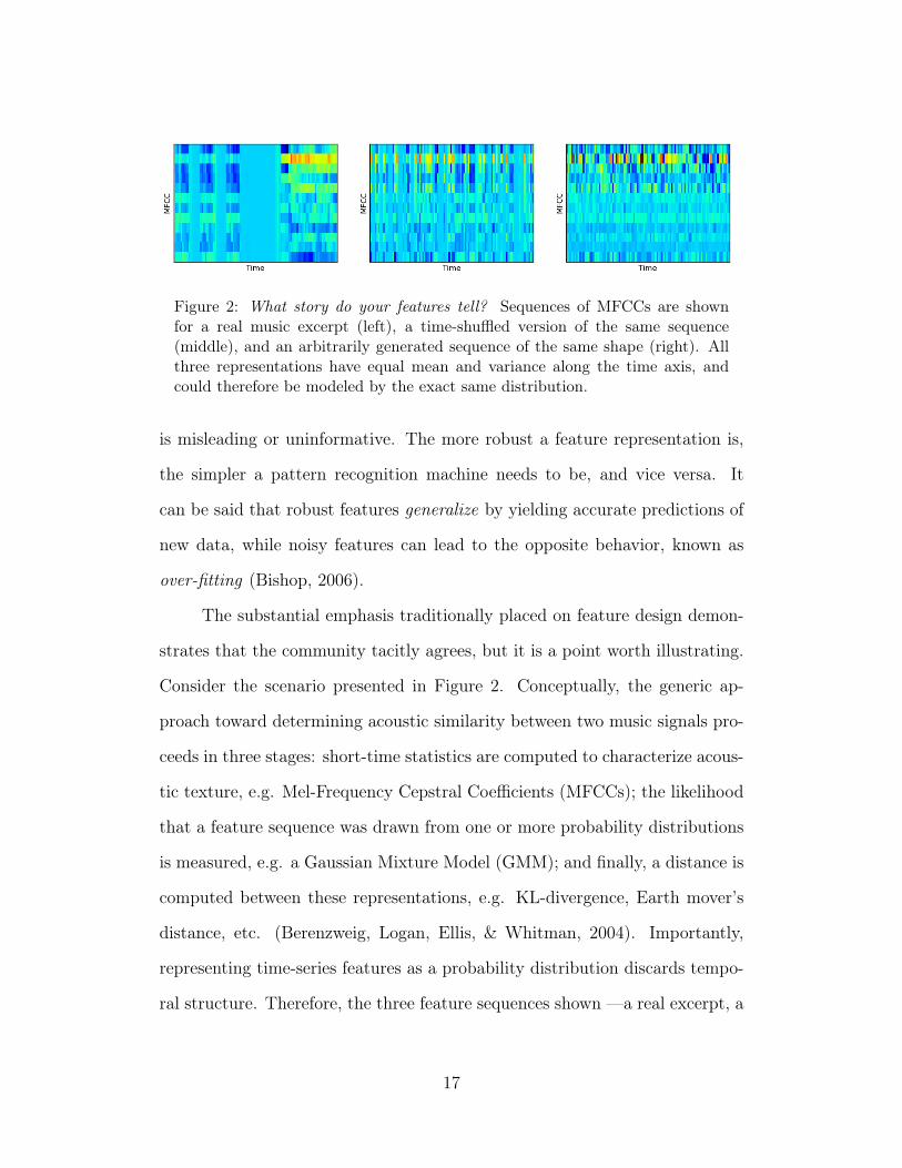
Figure 2: What story do your features tell? Sequences of MFCCs are shownfor a real music excerpt (left), a time-shuffled version of the same sequence(middle), and an arbitrarily generated sequence of the same shape (right). Allthree representations have equal mean and variance along the time axis, andcould therefore be modeled by the exact same distribution.
is misleading or uninformative. The more robust a feature representation is,
the simpler a pattern recognition machine needs to be, and vice versa. It
can be said that robust features generalize by yielding accurate predictions of
new data, while noisy features can lead to the opposite behavior, known as
over-fitting (Bishop, 2006).
The substantial emphasis traditionally placed on feature design demon-
strates that the community tacitly agrees, but it is a point worth illustrating.
Consider the scenario presented in Figure 2. Conceptually, the generic ap-
proach toward determining acoustic similarity between two music signals pro-
ceeds in three stages: short-time statistics are computed to characterize acous-
tic texture, e.g. Mel-Frequency Cepstral Coefficients (MFCCs); the likelihood
that a feature sequence was drawn from one or more probability distributions
is measured, e.g. a Gaussian Mixture Model (GMM); and finally, a distance is
computed between these representations, e.g. KL-divergence, Earth mover’s
distance, etc. (Berenzweig, Logan, Ellis, & Whitman, 2004). Importantly,
representing time-series features as a probability distribution discards tempo-
ral structure. Therefore, the three feature sequences shown —a real excerpt, a
17
shuffled version of it, and a randomly generated one with the same statistics—
are identical in the eyes of such a model. The audio that actually corresponds
to these respective representations, however, will certainly not sound similar
to a human listener.
This bears a significant consequence: any ambiguity introduced or irrel-
evant variance left behind in the process of computing features must instead
be resolved by the pattern recognition machine. Previous research in chord
estimation has explicitly shown that better features allow for simpler classifiers
(Cho, Weiss, & Bello, 2010), and intuitively many have spent years steadily
improving their respective feature extraction implementations (Lyon, Rehn,
Bengio, Walters, & Chechik, 2010; Müller & Ewert, 2011). Moreover, there is
ample evidence these various classification strategies work quite well on myriad
problems and datasets (Bishop, 2006). The logical conclusion to draw from
this observation is that underperforming automatic music description systems
are more likely the result of deficiencies in the feature representation than the
classifier applied to it.
It is particularly prudent then, to examine the assumptions and design
decisions incorporated into feature extraction systems. In music signal process-
ing, audio feature extraction typically consists of a recombination of a small
set of operations, as depicted in Figure 3: splitting the signal into indepen-
dent short-time segments, referred to as blocks or frames; applying an affine
transformation, generally interpreted as either a projection or filterbank; ap-
plying a point-wise nonlinear function; and pooling across frequency or time.
These operations can be, and often are, repeated in the process. For example,
MFCCs are computed by filtering a signal segment at multiple frequencies on a
Mel-scale (affine transform), taking the logarithm (a nonlinearity), and apply-
18
Affine Transformation
Constant-Q Filterbank
Mel-scaleFilterbank
Non-linearity
Modulus /Log-Scaling
Modulus /Log-Scaling
Pooling
Octave Equivalnce
Affine Transformation
Discrete Cosine Projection
Features
Chroma
MFCC
Short-timeWindowingAudio Signal
≈ 800ms
≈ 50ms
Figure 3: State of the art : Standard approaches to feature extraction proceedas the cascaded combination of a few simpler operations; on closer inspection,the main difference between chroma and MFCCs is the parameters used.
ing the Discrete Cosine Transform (another affine transformation). Similarly,
chroma features are produced by applying a constant-Q filterbank (affine trans-
formation), taking the complex modulus of the coefficients (non-linearity), and
summing across octaves (pooling).
Considering this formulation, there are three specific reasons why this
approach might be problematic. First, though the data-driven training of
classifiers and other pattern recognition machines has been standard for over
a decade in music informatics, the parametrization of feature extractors —e.g.
choice of filters, non-linearities and pooling strategies, and the order in which
they are applied— remains, by and large, a manual process. Both feature ex-
traction and classifier training present the same basic problem: there exists a
large space of possible signal processing systems and, somewhere in it, a config-
uration that optimizes an objective function over a dataset. Though the music
informatics community is privileged with a handful of talented researchers who
are particularly adept at exploring this daunting space, crafting good features
can be a time consuming and non-trivial task. Additionally, carefully tuning
features for one specific application offers no guarantees about relevance or
versatility in another scenario. As a result, features developed for one task
19
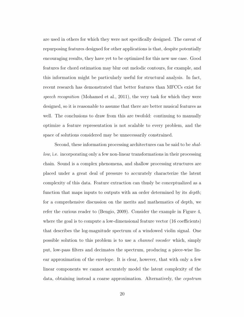
are used in others for which they were not specifically designed. The caveat of
repurposing features designed for other applications is that, despite potentially
encouraging results, they have yet to be optimized for this new use case. Good
features for chord estimation may blur out melodic contours, for example, and
this information might be particularly useful for structural analysis. In fact,
recent research has demonstrated that better features than MFCCs exist for
speech recognition (Mohamed et al., 2011), the very task for which they were
designed, so it is reasonable to assume that there are better musical features as
well. The conclusions to draw from this are twofold: continuing to manually
optimize a feature representation is not scalable to every problem, and the
space of solutions considered may be unnecessarily constrained.
Second, these information processing architectures can be said to be shal-
low, i.e. incorporating only a few non-linear transformations in their processing
chain. Sound is a complex phenomena, and shallow processing structures are
placed under a great deal of pressure to accurately characterize the latent
complexity of this data. Feature extraction can thusly be conceptualized as a
function that maps inputs to outputs with an order determined by its depth;
for a comprehensive discussion on the merits and mathematics of depth, we
refer the curious reader to (Bengio, 2009). Consider the example in Figure 4,
where the goal is to compute a low-dimensional feature vector (16 coefficients)
that describes the log-magnitude spectrum of a windowed violin signal. One
possible solution to this problem is to use a channel vocoder which, simply
put, low-pass filters and decimates the spectrum, producing a piece-wise lin-
ear approximation of the envelope. It is clear, however, that with only a few
linear components we cannot accurately model the latent complexity of the
data, obtaining instead a coarse approximation. Alternatively, the cepstrum
20

Figure 4: Low-order approximations of highly non-linear data: The log-magnitude spectra of a violin signal (black) is characterized by a channel vocoder(blue) and cepstrum coefficients (green). The latter, being a higher-order func-tion, is able to more accurately describe the contour with the same number ofcoefficients.
method transforms the log-magnitude spectrum before low-pass filtering. In
this case, the increase in depth allows the same number of coefficients to more
accurately represent the envelope. Obviously, powerful pattern recognition
machines can be used in an effort to compensate for the deficiencies of a fea-
ture representation. However, shallow, low-order functions are fundamentally
limited in the kinds of behavior they can characterize, and this is problematic
when the complexity of the data greatly exceeds the complexity of the model.
Third, short-time signal analysis is intuitively problematic because the
vast majority of our musical experiences do not live in hundred millisecond
intervals, but at least on the order of seconds or minutes. Conventionally,
features derived from short-time signals are limited to the information content
contained within each segment. As a result, if some musical event does not
occur within the span of an observation —a motif that does not fit within a
single frame— then it simply cannot be described by that feature vector alone.
This is clearly an obstacle to capturing high-level information that unfolds over
longer durations, noting that time is extremely, if not fundamentally, impor-
tant to how music is perceived. Admittedly, it is not immediately obvious how
21
to incorporate longer, or even multiple, time scales into a feature representa-
tion, with previous efforts often taking one of a few simple forms. Shingling
is one such approach, where a consecutive series of features is concatenated
into a single, high-dimensional vector (Casey, Rhodes, & Slaney, 2008). In
practice, shingling can be fragile to even slight translations that may arise
from tempo or pitch modulations. Alternatively, bag-of-frames (BoF) models
consider patches of features, fitting the observations to a probability distribu-
tion. As addressed earlier with Figure 2, bagging features discards temporal
structure, such that any permutation of the feature sequence yields the same
distribution. The most straightforward technique is to ignore longer time scales
at the feature level altogether, relying on post-filtering after classification to
produce more musically plausible results. For this to be effective though, the
musical object of interest must live at the time-scale of the feature vector or it
cannot truly be encoded. Ultimately, none of these approaches are well suited
to characterizing structure over musically meaningful time-scales.
1.1 A Concise Summary of Current Obstacles
In an effort to understand why progress in content-based music informatics
may be plateauing, the standard approach to music signal processing and
feature design has been reviewed, deconstructing assumptions and motivations
behind various decisions. As a result, three potential areas of improvement are
identified. So that each may be addressed in turn, it is useful to succinctly
restate the main points of this section:
• Hand-crafted feature design is neither scalable nor sustainable:
Framing feature design as a search in a solution space, the goal is to
22
discover the configuration that optimizes an objective function. Even
conceding that some gifted researchers might be able to achieve this on
their own, they are too few and the process too time-consuming to real-
istically solve every feature design challenge that will arise.
• Shallow processing architectures struggle to describe the latent
complexity of real-world phenomena: Feature extraction is similar
in principle to compactly approximating functions. Real data, however,
lives on a highly non-linear manifold and shallow, low-order functions
have difficulty describing this information accurately.
• Short-time analysis cannot naturally capture higher level in-
formation: Despite the importance of long-term structure in music,
features are predominantly derived from short-time segments. These
statistics cannot capture information beyond the scope of its observa-
tion, and common approaches to characterizing longer time scales are
ill-suited to music.
2 Deep Learning: A Slightly Different Direction
Looking toward how the research community might begin to address these
specific shortcomings in modern music signal processing, there is an important
development currently underway in computer science. Deep learning is riding a
wave of promise and excitement in multiple domains, toppling a variety of long-
standing benchmarks (Krizhevsky, Sutskever, & Hinton, 2012; G. Hinton et
23
al., 2012), while slowly permeating the public lexicon(Brumfiel, 2014; Markoff,
2012). Despite all the attention, however, this approach to solving machine
perception problems has yet to gain significant traction in content-based music
informatics. Before attempting to formally define deep learning, though, it is
useful to break down the ideas behind the very name itself and develop an
intuition as to why this area is of particular interest.
2.1 Deep Architectures
It was previously shown that deeper processing structures are better suited to
characterize complex data. Such systems can be difficult to design, however,
as it can be challenging to decompose an abstract music intelligence task into
a logical cascade of operations. That said, the evolution of tempo estima-
tion systems is a perfect example of a deep signal processing structure that
developed naturally in the due course of research.
The high-level design intuition behind a tempo tracking system is rela-
tively straightforward and, as evidenced by various approaches, widely agreed
upon. First, the occurrence of musical events, or onsets, are identified, and
then the underlying periodicity is estimated. The earliest efforts in tempo
analysis tracked symbolic events (Dannenberg, 1984), but it was soon shown
that a time-frequency representation of sound was useful in encoding rhythmic
information (Scheirer, 1998). This led to in-depth studies of onset detection
(Bello et al., 2005), based on the idea that “good” impulse-like signals, referred
to as novelty functions, would greatly simplify periodicity analysis. Along the
way, it was also discovered that applying non-linear compression to a nov-
elty function produced noticeably better results (A. P. Klapuri, Eronen, &
Astola, 2006). Various periodicity tracking methods were simultaneously ex-
24
SubbandDecomposition
OnsetDetection
PeriodicityAnalysis
Audio
Transformation
Rectification
Non-linearCompression
Pooling
Time-Frequency Representation
Novelty Function
Tempo Spectra
Argmax
Figure 5: A complex system of simple parts: Tempo estimation has, over time,naturally converged to a deep architecture. Note how each processing layerabsorbs a different type of variance —pitch, absolute amplitude, and phase— totransform two different signals into nearly identical representations.
plored, including oscillators (Edward & Kolen, 1994), multiple agents (Goto
& Muraoka, 1995), inter-onset interval histograms (Dixon, 2007), and tuned
filterbanks (Grosche & Müller, 2011).
Reflecting on this lineage, system design has, over time, converged to a
deep learning architecture, minus the learning, where the same processing ele-
ments —filtering and transforms, non-linearities, and pooling— are replicated
over multiple processing layers. Interestingly, as shown in Figure 5, visual in-
spection demonstrates why it is particularly well suited to the task of tempo
estimation. Consider two input waveforms with little in common but tempo;
one, an ascending D Major scale played on a trumpet, and the other, a de-
layed series of bass drum hits. It can be seen that, at each layer, a different
kind of variance in the signal is removed. The filterbank front-end absorbs
rapid fluctuations in the time-domain signal, spectrally separating acoustic
events. This facilitates onset detection, which provides a pitch and timbre
25
invariant estimate of events in the signal, reducing information along the fre-
quency dimension. Lastly, periodicity analysis eliminates shifts in the pulse
train by discarding phase information. At the output of the system, these
two acoustically different inputs have been transformed into nearly identical
representations. Therefore, the most important lesson demonstrated by this
example is how invariance can be achieved by distributing complexity over
multiple processing layers.
As mentioned, not all tasks share the same capacity for intuition. Multi-
level wavelet filterbanks, referred to as scattering transforms, have also shown
promise as a general deep architecture for audio classification by capturing
information over not only longer, but also multiple, time-scales (Andén &
Mallat, 2011). Recognizing MFCCs as a first-order statistic, this second-order
system yielded better classification results over the same observation length
while also achieving convincing reconstruction of the original signals. The au-
thors demonstrate their approach to be a multi-layer generalization of MFCCs,
and exhibit strong parallels to certain deep network architectures, although the
parameterization here is not learned but defined. Perhaps a more intriguing
observation to draw from this work though is the influence a fresh perspec-
tive can have on designing deep architectures. Rather than propagating all
information upwards through the structure, the system keeps summary statis-
tics at each timescale, demonstrating better performance in the applications
considered.
2.2 Feature Learning
In traditional music informatics systems, features are tuned manually, lever-
aging human insight and intuition, and classifiers are tuned automatically,
26
leveraging an objective criterion and numerical optimization. For this reason,
the quality of hand-crafted features is a crucial aspect of system design, as nu-
merical optimization occurs downstream of manual feature design. Many are
well aware of the value inherent to good representations, and feature tuning
has become a common, if tedious, component in music informatics research.
One such instance where this has occurred is in the tuning of chroma features.
Developed by Fujishima around the turn of the century (Fujishima, 1999),
the last decade and a half has seen consistent iteration and improvement on
the same basic concept; estimate the contribution of each pitch class over a
short-time observation of audio. Though initially devised for chord estimation,
chroma features have been used in a variety of applications, such as struc-
tural segmentation (Levy, Noland, & Sandler, 2007) or version identification
(Salamon, Serra, & Gómez, 2013).
The fundamental goal in computing chroma features is to consolidate
the energies of each pitch class according to a particular magnitude frequency
representation. One of the simplest ways to do so, given in Figure 6-(a), shows
the averaging of pitch classes in a constant-Q filterbank, e.g. frequencies are
spaced like the keys of a piano. Later developments found that weighting the
contributions of each frequency with a Gaussian window led to better perfor-
mance, as shown in Figure 6-(b) (Cho, 2014). This improvement still took
time to develop, further motivating the notion that other simple modifications
remain undiscovered. That said, this knowledge is attained by maximizing a
known objective measure, such as classification accuracy in a chord estimation
task. Reflecting, this begs an obvious question: perhaps the parameters of a
chroma estimation function could instead be learned via numerical optimiza-
tion?
27
(a)
C1 C2 C3 C4 C5 C6 C7
CC#DEbEF
F#GAbABbB
(b)
C1 C2 C3 C4 C5 C6 C7
CC#DEbEF
F#GAbABbB
(c)
C1 C2 C3 C4 C5 C6 C7
CC#DEbEF
F#GAbABbB
Figure 6: Various weight matrices for computing chroma features, correspondingto (a) uniform average, (b) Gaussian-weighted average, and (c) learned weights;red corresponds to positive values, blue to negative.
28
Manual
CC#DEbEF
F#GAbABbB
Time
Learn
ed
CC#DEbEF
F#GAbABbB
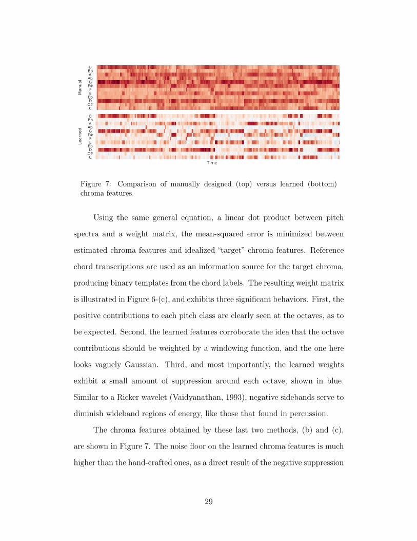
Figure 7: Comparison of manually designed (top) versus learned (bottom)chroma features.
Using the same general equation, a linear dot product between pitch
spectra and a weight matrix, the mean-squared error is minimized between
estimated chroma features and idealized “target” chroma features. Reference
chord transcriptions are used as an information source for the target chroma,
producing binary templates from the chord labels. The resulting weight matrix
is illustrated in Figure 6-(c), and exhibits three significant behaviors. First, the
positive contributions to each pitch class are clearly seen at the octaves, as to
be expected. Second, the learned features corroborate the idea that the octave
contributions should be weighted by a windowing function, and the one here
looks vaguely Gaussian. Third, and most importantly, the learned weights
exhibit a small amount of suppression around each octave, shown in blue.
Similar to a Ricker wavelet (Vaidyanathan, 1993), negative sidebands serve to
diminish wideband regions of energy, like those that found in percussion.
The chroma features obtained by these last two methods, (b) and (c),
are shown in Figure 7. The noise floor on the learned chroma features is much
higher than the hand-crafted ones, as a direct result of the negative suppression
29
in the learned weights. While the idea of adjacent pitch energy suppression is
novel, it is important to recognize a few things about this example. Most im-
portantly, it is curious to consider what other design aspects “learning” might
help tease out from data. The function considered here, a linear dot product,
is very constrained, and “better” features are likely possible through more com-
plex models. Additionally, it is possible to directly inspect the learned weights
because the system is straightforward; more complex models, however, will
make this process far more difficult.
2.3 Previous Deep Learning Efforts in Music Informatics
While far from widespread, an increasing number of researchers have begun
investigating deep learning to challenges in content-based music informatics.
The most common form of deep learning explored for music applications fo-
cuses on such models to single frames of a music signal for genre recogni-
tion (Hamel, Wood, & Eck, 2009), mood estimation (Schmidt & Kim, 2011),
note transcription (Nam, Ngiam, Lee, & Slaney, 2011), and artist recognition
(Dieleman, Brakel, & Schrauwen, 2011). Meanwhile, the earliest instance of
modern deep learning methods applied to music signals is found in the use
of convolutional networks for the detection of onsets (Lacoste & Eck, 2007).
More recently, convolutional networks have also been explored for genre recog-
nition (Li, Chan, & Chun, 2010), instrument similarity (Humphrey, Glennon,
& Bello, 2011), chord estimation (Humphrey, Cho, & Bello, 2012; Humphrey
& Bello, 2012), onset detection (Schluter & Bock, 2014), and structural seg-
mentation (Ullrich, Schlüter, & Grill, 2014). Recursive neural networks, a
powerful, if troublesome, model for sequential data, have also found success in
chord transcription (Boulanger-Lewandowski, Bengio, & Vincent, 2013) and
30
polyphonic pitch analysis (Sigtia et al., 2014). Additionally, predictive sparse
decomposition (PSD) and other methods inspired by sparse coding have also
seen a spike in interest (Henaff, Jarrett, Kavukcuoglu, & LeCun, 2011; Nam,
Herrera, Slaney, & Smith, 2012), but while they make use of learning, neither
of these systems are particularly deep. Regardless, it is worthwhile to note
that many, if not all, of these works have attained state of the art performance
on their respective tasks, often in the first application of the method to the
area.
3 Discussion
Recognizing slowing progress across various application areas in content-based
music informatics, this chapter has attempted to develop an understanding as
to why this might be the case. Revisiting common approaches to the design of
music signal processing systems revealed three possible shortcomings: manual
feature design cannot scale to every problem the field will need to solve; many
architectures are too shallow to adequately model the complexity of the data;
and there currently are not many good answers for handling longer time-scales.
In looking to other related disciplines, it seems deep learning may help
address some, if not all, of these challenges. Deep architectures are able to
distribute complexity across multiple processing layers, thus being able to
model more complex data. Feature learning, on the other hand, allows for
the automatic optimization of known objective functions, making it easier to
discover signal-level characteristics relevant to a given task faster. In fact, a
handful of previous deep learning efforts within music informatics have already
begun to demonstrate the promise of such methods.
31
Notably, these are crucial observations to make now for a variety of
reasons. From a practical standpoint, many in the research community are
investing considerable effort in the curation of datasets. While some, like
(Bittner et al., 2014), have gone to great lengths to clear licenses for the
source audio signals, most use commercial recordings and thus sharing the
original content is problematic. As a result, it is becoming standard practice
to apply a respected, but non-invertible, feature extraction algorithm over the
original audio content and share the extracted statistics with the community,
e.g. the Million Song Dataset (Bertin-Mahieux, Ellis, Whitman, & Lamere,
2011). While these efforts are commendable, such datasets are ultimately
limited by the feature extraction algorithm employed.
32
CHAPTER III
DEEP LEARNING
Deep learning descends from a long and, at times, rocky history of ar-
tificial intelligence, information theory, and computer science. The goals of
the this chapter are two-fold: Section 2 first offers a concise summary of the
history of deep learning in three parts, detailing the origins, critical advances,
and current state of the art of neural networks. Afterwards, a formal treat-
ment of deep learning is addressed in three parts: Section 2.1 introduces the
architectural components of deep networks; Section 2.2 introduces the process
of automatic learning, covering the design of loss functions and basic theory
of gradient-based optimization; and Section 2.3 outlines various tricks of the
trade and other practical considerations in the use of deep learning. Finally,
the concepts introduced in this chapter are briefly summarized in Section 3.
1 A Brief History of Neural Networks
Despite the recent wave of interest and excitement surrounding it, the core
principles of deep learning were originally devised halfway through the 20th
century, grounded in mathematics established even earlier. As a direct descen-
dant of neural networks —computational models with an ambitious moniker
burdened by a tumultuous past— the very mention of deep learning often el-
licts several warranted, if suspicious, questions: What’s the difference? What’s
changed? Why do they suddenly work now? Thus, before diving into a formal
33
review of the deep learning and its various components, it is worthwhile to
contextualize the research trajectory that has led to today.
1.1 Origins (pre-1980)
For Western Europe and those in its sphere of influence, the Age of Enlighten-
ment marked a golden era of human knowledge, consisting of great advances
in many diverse fields, such as mathematics, philosophy, and the physical
sciences. Long had humanity contemplated the notions of consciousness and
reasoning, but here brilliant thinkers began to return to and explore these con-
cepts with resolve. From the efforts of scholars like Gottfried Leibnitz, Thomas
Hobbes, and George Boole, formal logic blossomed into its own mathemati-
cal discipline. In doing so, it became possible to symbolically express the
act of reasoning, whereby rational thought could be described by a system of
equations to be transformed or even solved.
It was this critical development —the idea of logical computation— that
encouraged subsequent generations to speculate on the apparent feasibility of
artificial intelligence. And, coinciding with the advent of electricity in the 20th
century, mathematicians, philosophers, and scientists of the modern era sought
to create machines that could think. While the space of relevant contributions
is too great to enumerate here, there were a handful of breakthroughs that
would prove integral to the field of computer science. In 1936, Alan Turing
devised the concept of a “universal machine”, which would lead to the proof
that a system of binary states, e.g. true and false, could be used to perform
any mathematical operation (Turing, 1936). Only shortly thereafter, Claude
Shannon demonstrated in his master’s thesis that Boolean logic could be im-
plemented in electrical circuits via switches and relays, forming the basis of
34
the modern computer (Shannon, 1938). Shortly thereafter, in 1943, McCulloch
and Pitts constructed the first artificial neuron, a simple computational model
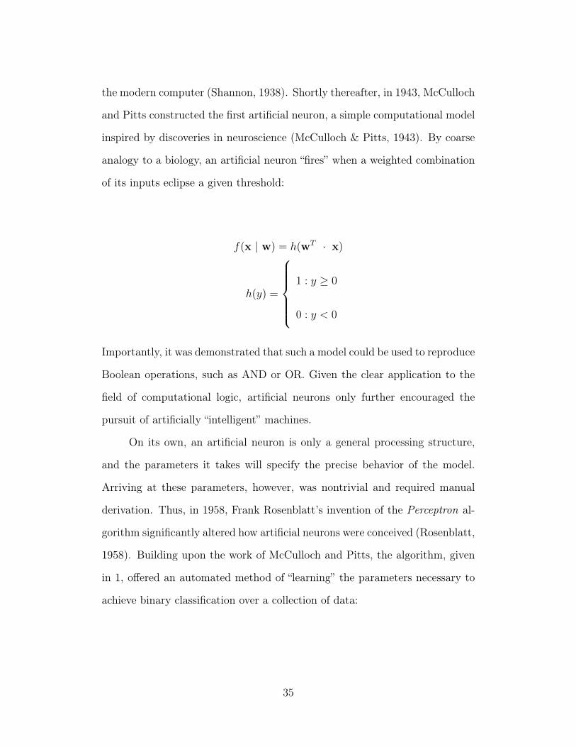
inspired by discoveries in neuroscience (McCulloch & Pitts, 1943). By coarse
analogy to a biology, an artificial neuron “fires” when a weighted combination
of its inputs eclipse a given threshold:
f(x | w) = h(wT · x)
h(y) =
1 : y ≥ 0
0 : y < 0
Importantly, it was demonstrated that such a model could be used to reproduce
Boolean operations, such as AND or OR. Given the clear application to the
field of computational logic, artificial neurons only further encouraged the
pursuit of artificially “intelligent” machines.
On its own, an artificial neuron is only a general processing structure,
and the parameters it takes will specify the precise behavior of the model.
Arriving at these parameters, however, was nontrivial and required manual
derivation. Thus, in 1958, Frank Rosenblatt’s invention of the Perceptron al-
gorithm significantly altered how artificial neurons were conceived (Rosenblatt,
1958). Building upon the work of McCulloch and Pitts, the algorithm, given
in 1, offered an automated method of “learning” the parameters necessary to
achieve binary classification over a collection of data:
35
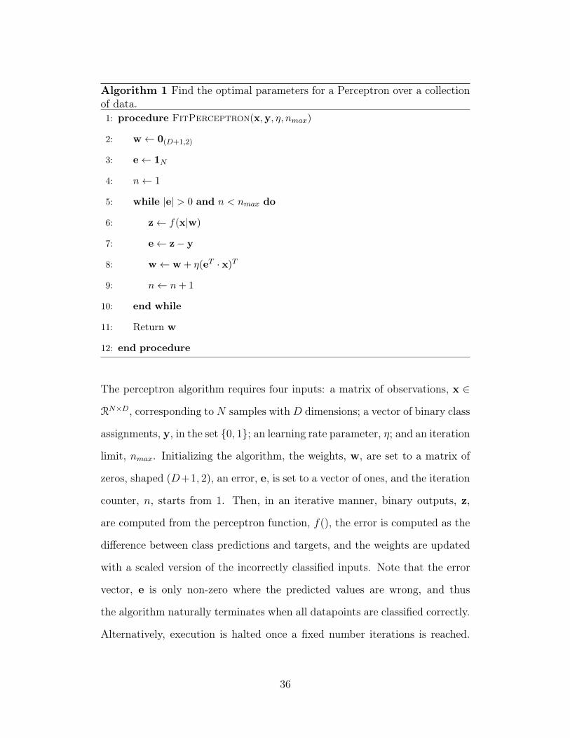
Algorithm 1 Find the optimal parameters for a Perceptron over a collectionof data.1: procedure FitPerceptron(x,y, η, nmax)
2: w← 0(D+1,2)
3: e← 1N
4: n← 1
5: while |e| > 0 and n < nmax do
6: z← f(x|w)
7: e← z− y
8: w← w + η(eT · x)T
9: n← n+ 1
10: end while
11: Return w
12: end procedure
The perceptron algorithm requires four inputs: a matrix of observations, x ∈
RN×D, corresponding to N samples withD dimensions; a vector of binary class
assignments, y, in the set {0, 1}; an learning rate parameter, η; and an iteration
limit, nmax. Initializing the algorithm, the weights, w, are set to a matrix of
zeros, shaped (D+1, 2), an error, e, is set to a vector of ones, and the iteration
counter, n, starts from 1. Then, in an iterative manner, binary outputs, z,
are computed from the perceptron function, f(), the error is computed as the
difference between class predictions and targets, and the weights are updated
with a scaled version of the incorrectly classified inputs. Note that the error
vector, e is only non-zero where the predicted values are wrong, and thus
the algorithm naturally terminates when all datapoints are classified correctly.
Alternatively, execution is halted once a fixed number iterations is reached.
36
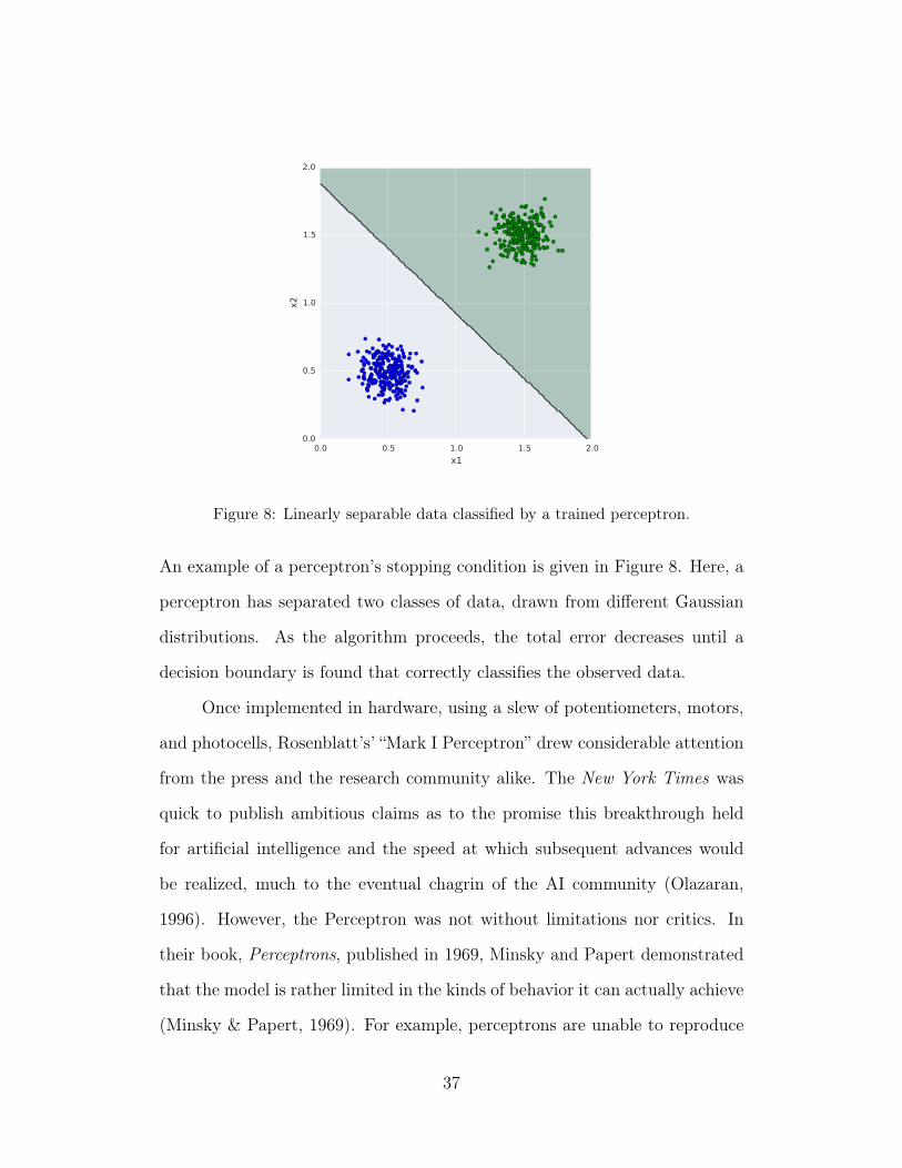
0.0 0.5 1.0 1.5 2.0
x1
0.0
0.5
1.0
1.5
2.0
x2
Figure 8: Linearly separable data classified by a trained perceptron.
An example of a perceptron’s stopping condition is given in Figure 8. Here, a
perceptron has separated two classes of data, drawn from different Gaussian
distributions. As the algorithm proceeds, the total error decreases until a
decision boundary is found that correctly classifies the observed data.
Once implemented in hardware, using a slew of potentiometers, motors,
and photocells, Rosenblatt’s’ “Mark I Perceptron” drew considerable attention
from the press and the research community alike. The New York Times was
quick to publish ambitious claims as to the promise this breakthrough held
for artificial intelligence and the speed at which subsequent advances would
be realized, much to the eventual chagrin of the AI community (Olazaran,
1996). However, the Perceptron was not without limitations nor critics. In
their book, Perceptrons, published in 1969, Minsky and Papert demonstrated
that the model is rather limited in the kinds of behavior it can actually achieve
(Minsky & Papert, 1969). For example, perceptrons are unable to reproduce
37
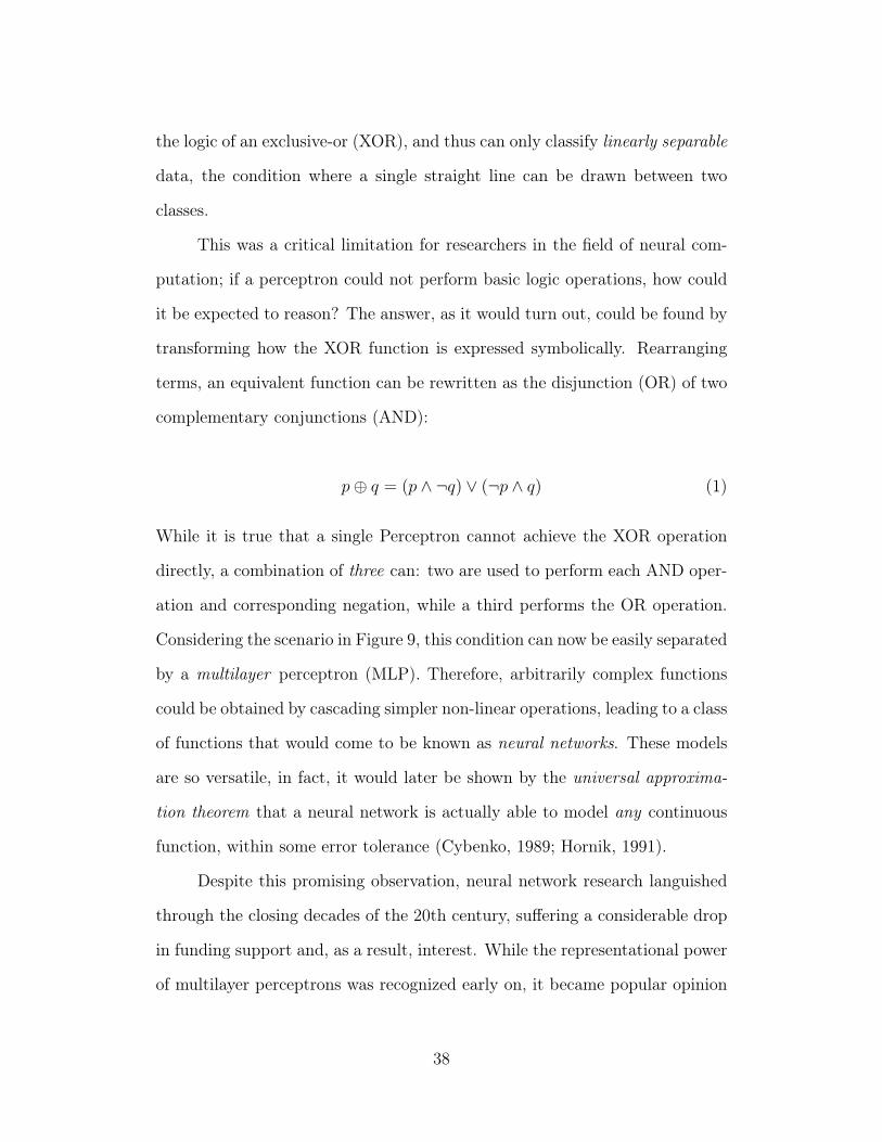
the logic of an exclusive-or (XOR), and thus can only classify linearly separable
data, the condition where a single straight line can be drawn between two
classes.
This was a critical limitation for researchers in the field of neural com-
putation; if a perceptron could not perform basic logic operations, how could
it be expected to reason? The answer, as it would turn out, could be found by
transforming how the XOR function is expressed symbolically. Rearranging
terms, an equivalent function can be rewritten as the disjunction (OR) of two
complementary conjunctions (AND):
p⊕ q = (p ∧ ¬q) ∨ (¬p ∧ q) (1)
While it is true that a single Perceptron cannot achieve the XOR operation
directly, a combination of three can: two are used to perform each AND oper-
ation and corresponding negation, while a third performs the OR operation.
Considering the scenario in Figure 9, this condition can now be easily separated
by a multilayer perceptron (MLP). Therefore, arbitrarily complex functions
could be obtained by cascading simpler non-linear operations, leading to a class
of functions that would come to be known as neural networks. These models
are so versatile, in fact, it would later be shown by the universal approxima-
tion theorem that a neural network is actually able to model any continuous
function, within some error tolerance (Cybenko, 1989; Hornik, 1991).
Despite this promising observation, neural network research languished
through the closing decades of the 20th century, suffering a considerable drop
in funding support and, as a result, interest. While the representational power
of multilayer perceptrons was recognized early on, it became popular opinion
38
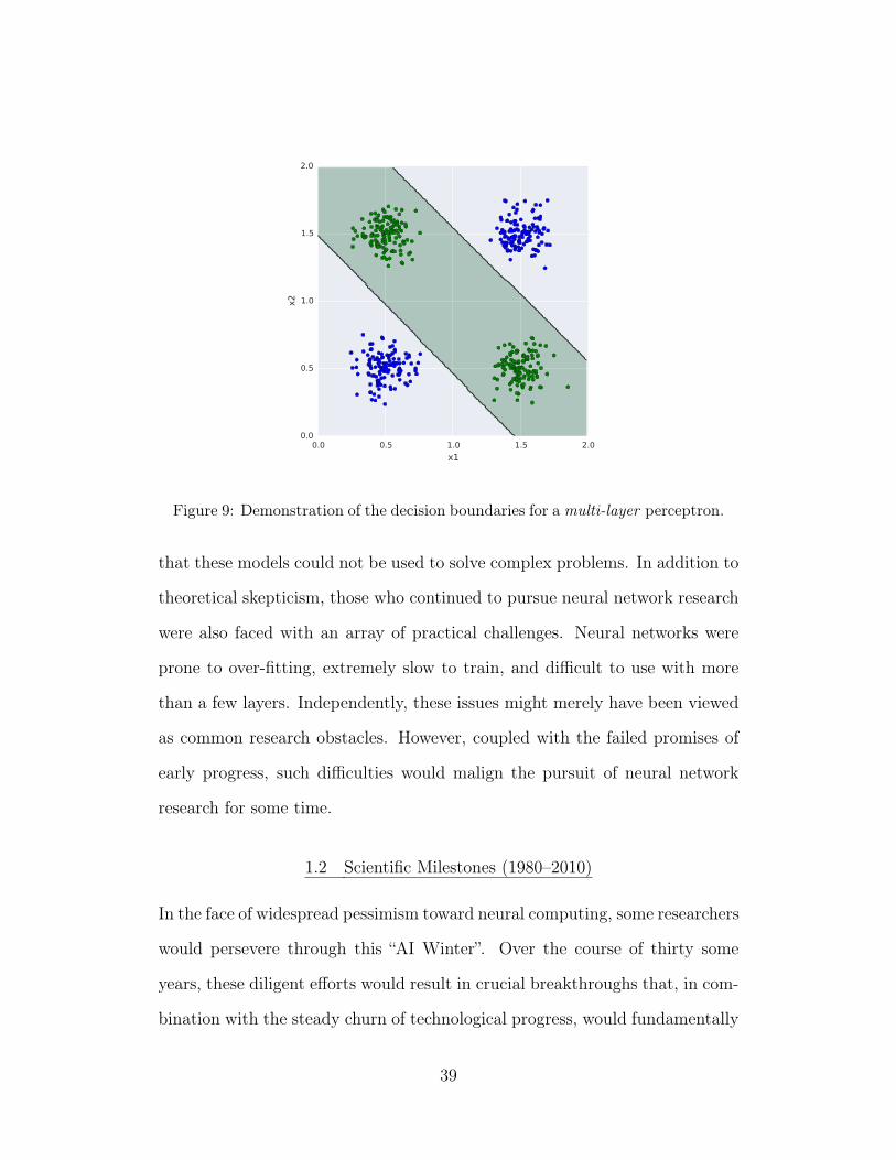
0.0 0.5 1.0 1.5 2.0
x1
0.0
0.5
1.0
1.5
2.0
x2
Figure 9: Demonstration of the decision boundaries for a multi-layer perceptron.
that these models could not be used to solve complex problems. In addition to
theoretical skepticism, those who continued to pursue neural network research
were also faced with an array of practical challenges. Neural networks were
prone to over-fitting, extremely slow to train, and difficult to use with more
than a few layers. Independently, these issues might merely have been viewed
as common research obstacles. However, coupled with the failed promises of
early progress, such difficulties would malign the pursuit of neural network
research for some time.
1.2 Scientific Milestones (1980–2010)
In the face of widespread pessimism toward neural computing, some researchers
would persevere through this “AI Winter”. Over the course of thirty some
years, these diligent efforts would result in crucial breakthroughs that, in com-
bination with the steady churn of technological progress, would fundamentally
39
change the landscape of neural network research. While no one facet can truly
be credited with reviving the field, each would play an integral role in helping
the research community again warm up to neural networks.
1.2.1 Efficient Error Backpropagation
Via the perceptron algorithm, a machine effectively “learns” to classify data
by finding parameters that optimize a given objective function. This learning
strategy must be modified in the multilayer case, as it is not possible to directly
update the parameters through the heaviside, or unit step, function. Early re-
searchers noted that if the discontinuous activation function is replaced with a
logistic, or sigmoid, the composite multilayer network is differentiable. Thus,
as will be discussed in more detail in Section 2.2.2, it is possible to use this
gradient information to optimize the parameters of a network given an ob-
jective fitness measure, effectively back-propagating error through the network
(G. E. Hinton, 1986).
This approach was not without its deficiencies, however. First and fore-
most, the error term was typically computed over the entire dataset, which
often proved computationally expensive for sufficiently large collections. Ad-
ditionally, early efforts found this particular approach often resulted in poor
answers, and struggled to update parameters of networks with many layers. In
time, a stochastic variant of this algorithm was shown to be far more efficient,
and even circumvented some of these issues (Y. A. LeCun, Bottou, Orr, &
Müller, 1998). Whereas conventional optimization occurs over an entire col-
lection of datapoints, this efficient version randomly subsamples the training
set and computes the error term over fewer datapoints. Though the error es-
40
timate is much noisier, the strategy is still effective, significantly faster, and
may even be less susceptible to bad parameters as a result.
1.2.2 Convolutional Neural Networks
Though equal parts remarkable and encouraging, the universal approximation
theorem has significant practical limitations. First, the theorem only holds
for a sufficiently, and perhaps infinitely, wide network. Additionally, it says
nothing about how one might parameterize such a function in order to achieve
some desired behavior. Thus, despite such overwhelming promise, early neural
networks often resulted in poor approximations of the functions being mod-
eled, because the flexibility of the model vastly surpassed the amount of data
available to train it. This flexibility was apparent in computer vision tasks, as
multilayer perceptrons struggled to cope with simple homographic deforma-
tions, such as translation, scaling, or rotation.
Natural vision systems, on the other hand, are quite robust to these
kinds of variation, and, as before, researchers looked to biology for inspira-
tion in modeling these processes. One particularly insightful study was that
of Hubel and Wiesel in 1959, who experimented on the neural behavior of
the feline visual cortex (Hubel & Wiesel, 1959). By presenting visual stimuli
while probing the brain with electrodes, they discovered two different kinds
of neurons —simple cells and complex cells— organized hierarchically. Ex-
perimental results indicated that the former is responsible for local feature
extraction, while the latter combines the inputs of simple cells to absorb small
amounts of variation in the observed stimuli.
These ideas were first incorporated in the Neocognitron of (Fukushima,
1988), and later realized successfully as a convolutional neural network for
41
shape recognition and handwritten digit classification (LeCun, Bottou, Ben-
gio, & Haffner, 1998), offering three key design features. Local receptive fields,
where compute features from a small neighborhood of pixels, exploiting the
observation that nearby pixel values tend to be highly correlated. Smaller
receptive fields require fewer parameters, thus reducing the overall size of the
model and the amount of data needed to train it. Applying local receptive
fields as a convolution results in effectively sharing the weights over all posi-
tions in an image. Thus weight sharing reduces the number of parameters even
further, while allowing the network to identify features regardless of position
in an image. Finally, max-pooling reduces small neighborhoods to the largest
value within it, introducing not only shift but a small amount of scale and
rotation invariance. Taken together, these advantageous attributes directly
resolved many of the issues plaguing multilayer perceptrons, and proved to be
the most successful instance of neural computing for nearly two decades.
1.2.3 Proliferation of Digital Data
Given the ubiquity of digital information in the modern era, it is easy to
forget that neural networks were first developed in a considerably different
day and age. The very existence of digital audio and images, for example,
did not become commonplace until the end of the 20th century. Even then,
these signals were costly to create, cumbersome to work with, and generally
difficult to share. Furthermore, once obtained, the process of annotating this
information for use in supervised learning requires a great deal of time and
effort. Thus, in the vein of speech recognition or computer vision for example,
machine perception research was forced to work with small datasets as a result.
Given the versatility of neural networks to model complex data, it was typically
42
trivial to over-fit these small training, while failing to generalize to new data.
Neural networks developed the reputation of being “data hungry”, requiring a
large amount of training data in order to do anything useful in practice.
While this was, and in some cases still is, a valid consideration for neural
networks, the problem of data scarcity is far less of an issue now. For many
well worn tasks, researchers have had ample time to curate massive labeled
datasets. In the late 1980s, LeCun et al oversaw the development of a hand-
written digit dataset, comprised of 60k 28x28 pixel images (Y. LeCun, Cortes,
& Burges, 1998); for comparison, the ImageNet dataset consists of millions
of tagged, high resolution images (Deng et al., 2009). Similar efforts have
been undertaken in the fields of speech recognition (Fisher, Doddington, &
Goudie-Marshall, 1986), face recognition (Huang, Ramesh, Berg, & Learned-
Miller, 2007), or natural language processing (Lewis, Yang, Rose, & Li, 2004),
to name only a few. Additionally, given the rise of the Internet, it became
possible to leverage a variety of information sources to obtain labeled data,
such as user-generated content, via Last.fm∗ or Twitter†, weak feedback sig-
nals, e.g. Pandora Radio‡, or even as a means of distributing the annotation
effort (Von Ahn, Blum, Hopper, & Langford, 2003). Combined, the range
of information available for large-scale supervised learning grew considerably,
diminishing the issues posed by data-hungry algorithms.
As a by-product of the global transition to the digital realm though, an
even larger portion of unlabeled data was at the disposal of machine learning
researchers. Coupling the easy availability of digital information with the idea
∗http://www.last.fm/†http://www.twitter.com/‡http://www.pandora.com/
43
that “the human brain isn’t really supervised”, much effort was invested in the
space of unsupervised learning algorithms. Finally, in 2006, one such method,
referred as contrastive divergence, was able to successfully exploit unlabeled
data to improve the performance of a neural network (G. E. Hinton, Osindero,
& Teh, 2006). Using a cascade of of undirected models, known as a Restricted
Boltzmann machine (RBM), a neural network was trained in a greedy, layer-
wise manner to reproduce realistic data. After this process of learning how
real data behaves, the model could be “fine-tuned” with a smaller amount of
labeled data to realize impressive, state of the art performance. Referred to
as “pre-training”, learning on unsupervised data allowed the model to discover
parameters closer to a good final solution. Though later discoveries would
demonstrate pre-training to be unnecessary under certain conditions (Zeiler et
al., 2013), this breakthrough was perhaps the first to forcefully recapture the
attention of the machine learning community.
1.2.4 Advances in Computing Technology
While enough cannot be said about the scientific contributions of neural net-
work researchers over the last 40 years, it is critical to appreciate how com-
puting technology has evolved over that time span. In the days of Rosenblatt
and Minsky, computers consisted of transistors visible to the naked eye, filled
entire rooms, and cost a small fortune. More recently, personal computers of
the 1980s had kilobytes of memory, central processing units (CPUs) operated
in the range of tens of megahertz, and were still far too expensive for all but
the elite or dedicated. Computation was still quite slow as a result, and thus
the process of training neural networks took an impressive amount of time. To
combat these difficulties, researchers often attempted to cut corners by using
44
smaller models, smaller datasets, and training with fewer iterations. Some-
what unsurprisingly, the common experience with neural networks was quite
unfavorable.
Eventually, technology would catch up to the theory. Hardware became
increasingly smaller, memory grew to the size of gigabytes, processors acceler-
ated for a time seemingly without bound, and the cost of computers dropped to
the point of near ubiquity. On the heels of these developments, other hardware
and tools were adapted to facilitate neural network research, such as paral-
lel computing with graphics processing units (GPUs) and accessible software
tools, e.g. Theano (Bergstra et al., 2010) or Torch (Collobert, Kavukcuoglu,
& Farabet, 2011). Combined, significantly better technology directly enabled
research at unprecedented scale, accelerating progress and relaxing computa-
tional constraints imposed by technical limitations.
1.3 Modern Rennaissance (post-2010)
Following the many key advances named above, deep learning quickly acceler-
ated into the academic, industrial, and public lexicon. It did not take long to
convince some research communities of the newfound promise of neural net-
works. In hardly any time at all, deep neural networks surpassed the state
of the art in automatic speech recognition, systems tuned over the course of
several decades (G. Hinton et al., 2012). Similarly compelling results were ob-
tained in computer vision (Krizhevsky et al., 2012) and natural language pro-
cessing (Sutskever, Martens, & Hinton, 2011). Acknowledging the usefulness
of such high-performing systems, companies like Google, Facebook, Microsoft,
IBM, and Baidu began investing in industrial strength deep learning teams
and infrastructure (Dean et al., 2012).
45
Complementing the migration of ideas and individuals from academia to
industry, the idea of “deep learning” and thinking machines has again struck
a chord with both the press and general public. Google’s research efforts
in 2012, for example, yielded a deep network that automatically learned the
concepts of “cats” and “human faces”, trained on millions of still video frames
from YouTube (Q. Le et al., 2012). Understandably, the story was picked
up by The New York Times and WIRED, among countless others, drawing
widespread attention. Coupled with charismatic interviews from many of the
field’s preeminent leaders, neural networks have been thrust back into the
limelight.
2 Core Concepts
Reflecting on the historical lineage of neural networks, it becomes apparent
that deep learning is not one single thing, but rather a collection of ideas
and approaches toward neural computing. Thus, to help define the scope and
limits of this work, this section introduces the fundamental components that
contribute to a modern definition of the topic. Here, “deep learning” is defined
as an approach to designing complex information processing systems, exhibit-
ing two key traits; one, discussed in Subsection 2.1, the system architecture
can be expressed as a composite nonlinear function, composed of many sim-
pler operations; and two, presented in Subsection 2.2, the parameters of this
function can be “learned” by combining an objective function with numerical
optimzation methods. Finally, modern neural network research has produced
a useful array of “tricks of the trade”, detailed in Subection 2.3, which often
help squeeze every last bit of performance from a model.
46
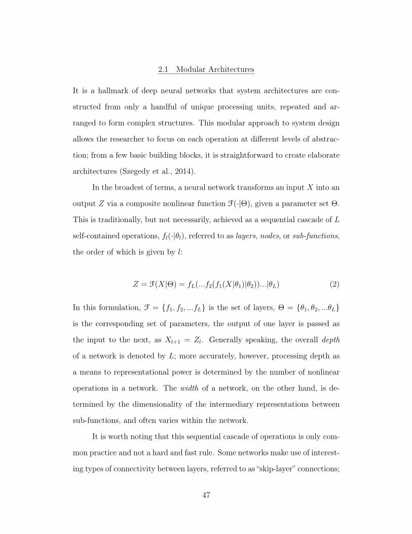
2.1 Modular Architectures
It is a hallmark of deep neural networks that system architectures are con-
structed from only a handful of unique processing units, repeated and ar-
ranged to form complex structures. This modular approach to system design
allows the researcher to focus on each operation at different levels of abstrac-
tion; from a few basic building blocks, it is straightforward to create elaborate
architectures (Szegedy et al., 2014).
In the broadest of terms, a neural network transforms an input X into an
output Z via a composite nonlinear function F(·|Θ), given a parameter set Θ.
This is traditionally, but not necessarily, achieved as a sequential cascade of L
self-contained operations, fl(·|θl), referred to as layers, nodes, or sub-functions,
the order of which is given by l:
Z = F(X|Θ) = fL(...f2(f1(X|θ1)|θ2))...|θL) (2)
In this formulation, F = {f1, f2, ...fL} is the set of layers, Θ = {θ1, θ2, ...θL}
is the corresponding set of parameters, the output of one layer is passed as
the input to the next, as Xl+1 = Zl. Generally speaking, the overall depth
of a network is denoted by L; more accurately, however, processing depth as
a means to representational power is determined by the number of nonlinear
operations in a network. The width of a network, on the other hand, is de-
termined by the dimensionality of the intermediary representations between
sub-functions, and often varies within the network.
It is worth noting that this sequential cascade of operations is only com-
mon practice and not a hard and fast rule. Some networks make use of interest-
ing types of connectivity between layers, referred to as “skip-layer” connections;
47
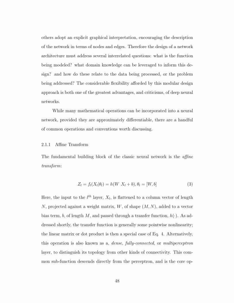
others adopt an explicit graphical interpretation, encouraging the description
of the network in terms of nodes and edges. Therefore the design of a network
architecture must address several interrelated questions: what is the function
being modeled? what domain knowledge can be leveraged to inform this de-
sign? and how do these relate to the data being processed, or the problem
being addressed? The considerable flexibility afforded by this modular design
approach is both one of the greatest advantages, and criticisms, of deep neural
networks.
While many mathematical operations can be incorporated into a neural
network, provided they are approximately differentiable, there are a handful
of common operations and conventions worth discussing.
2.1.1 Affine Transform
The fundamental building block of the classic neural network is the affine
transform:
Zl = fl(Xl|θl) = h(W Xl + b), θl = [W, b] (3)
Here, the input to the lth layer, Xl, is flattened to a column vector of length
N , projected against a weight matrix, W , of shape (M,N), added to a vector
bias term, b, of lengthM , and passed through a transfer function, h(·). As ad-
dressed shortly, the transfer function is generally some pointwise nonlinearity;
the linear matrix or dot product is then a special case of Eq. 4. Alternatively,
this operation is also known as a, dense, fully-connected, or multiperceptron
layer, to distinguish its topology from other kinds of connectivity. This com-
mon sub-function descends directly from the perceptron, and is the core op-
48
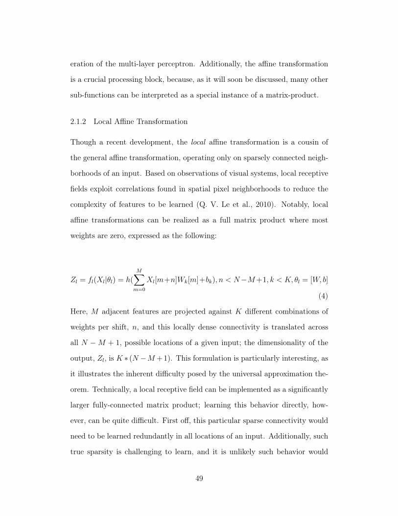
eration of the multi-layer perceptron. Additionally, the affine transformation
is a crucial processing block, because, as it will soon be discussed, many other
sub-functions can be interpreted as a special instance of a matrix-product.
2.1.2 Local Affine Transformation
Though a recent development, the local affine transformation is a cousin of
the general affine transformation, operating only on sparsely connected neigh-
borhoods of an input. Based on observations of visual systems, local receptive
fields exploit correlations found in spatial pixel neighborhoods to reduce the
complexity of features to be learned (Q. V. Le et al., 2010). Notably, local
affine transformations can be realized as a full matrix product where most
weights are zero, expressed as the following:
Zl = fl(Xl|θl) = h(M∑
m=0
Xl[m+n]Wk[m]+bk), n < N−M+1, k < K, θl = [W, b]
(4)
Here, M adjacent features are projected against K different combinations of
weights per shift, n, and this locally dense connectivity is translated across
all N −M + 1, possible locations of a given input; the dimensionality of the
output, Zl, is K ∗ (N −M + 1). This formulation is particularly interesting, as
it illustrates the inherent difficulty posed by the universal approximation the-
orem. Technically, a local receptive field can be implemented as a significantly
larger fully-connected matrix product; learning this behavior directly, how-
ever, can be quite difficult. First off, this particular sparse connectivity would
need to be learned redundantly in all locations of an input. Additionally, such
true sparsity is challenging to learn, and it is unlikely such behavior would
49
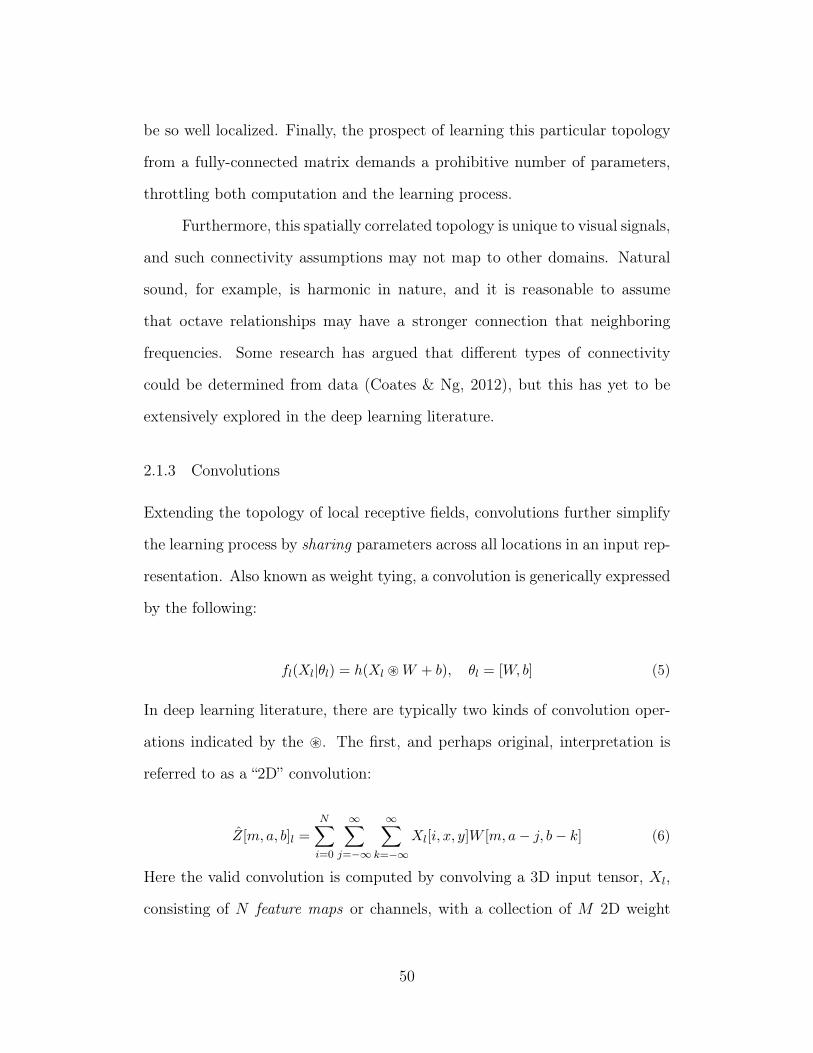
be so well localized. Finally, the prospect of learning this particular topology
from a fully-connected matrix demands a prohibitive number of parameters,
throttling both computation and the learning process.
Furthermore, this spatially correlated topology is unique to visual signals,
and such connectivity assumptions may not map to other domains. Natural
sound, for example, is harmonic in nature, and it is reasonable to assume
that octave relationships may have a stronger connection that neighboring
frequencies. Some research has argued that different types of connectivity
could be determined from data (Coates & Ng, 2012), but this has yet to be
extensively explored in the deep learning literature.
2.1.3 Convolutions
Extending the topology of local receptive fields, convolutions further simplify
the learning process by sharing parameters across all locations in an input rep-
resentation. Also known as weight tying, a convolution is generically expressed
by the following:
fl(Xl|θl) = h(Xl ~W + b), θl = [W, b] (5)
In deep learning literature, there are typically two kinds of convolution oper-
ations indicated by the ~. The first, and perhaps original, interpretation is
referred to as a “2D” convolution:
Z[m, a, b]l =N∑i=0
∞∑j=−∞
∞∑k=−∞
Xl[i, x, y]W [m, a− j, b− k] (6)
Here the valid convolution is computed by convolving a 3D input tensor, Xl,
consisting of N feature maps or channels, with a collection of M 2D weight
50
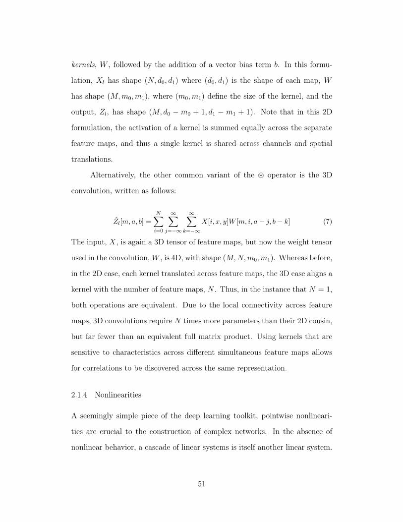
kernels, W , followed by the addition of a vector bias term b. In this formu-
lation, Xl has shape (N, d0, d1) where (d0, d1) is the shape of each map, W
has shape (M,m0,m1), where (m0,m1) define the size of the kernel, and the
output, Zl, has shape (M,d0 − m0 + 1, d1 − m1 + 1). Note that in this 2D
formulation, the activation of a kernel is summed equally across the separate
feature maps, and thus a single kernel is shared across channels and spatial
translations.
Alternatively, the other common variant of the ~ operator is the 3D
convolution, written as follows:
Zl[m, a, b] =
N∑i=0
∞∑j=−∞
∞∑k=−∞
X[i, x, y]W [m, i, a− j, b− k] (7)
The input, X, is again a 3D tensor of feature maps, but now the weight tensor
used in the convolution,W , is 4D, with shape (M,N,m0,m1). Whereas before,
in the 2D case, each kernel translated across feature maps, the 3D case aligns a
kernel with the number of feature maps, N . Thus, in the instance that N = 1,
both operations are equivalent. Due to the local connectivity across feature
maps, 3D convolutions require N times more parameters than their 2D cousin,
but far fewer than an equivalent full matrix product. Using kernels that are
sensitive to characteristics across different simultaneous feature maps allows
for correlations to be discovered across the same representation.
2.1.4 Nonlinearities
A seemingly simple piece of the deep learning toolkit, pointwise nonlineari-
ties are crucial to the construction of complex networks. In the absence of
nonlinear behavior, a cascade of linear systems is itself another linear system.
51
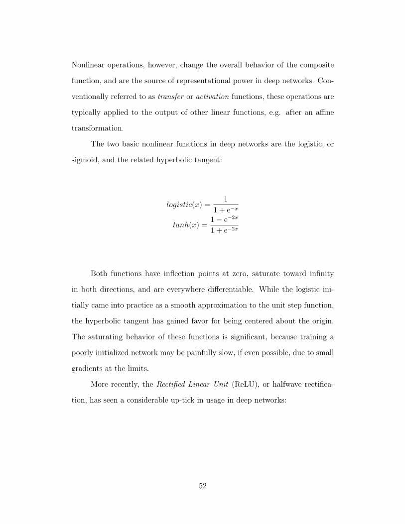
Nonlinear operations, however, change the overall behavior of the composite
function, and are the source of representational power in deep networks. Con-
ventionally referred to as transfer or activation functions, these operations are
typically applied to the output of other linear functions, e.g. after an affine
transformation.
The two basic nonlinear functions in deep networks are the logistic, or
sigmoid, and the related hyperbolic tangent:
logistic(x) =1
1 + e−x
tanh(x) =1− e−2x
1 + e−2x
Both functions have inflection points at zero, saturate toward infinity
in both directions, and are everywhere differentiable. While the logistic ini-
tially came into practice as a smooth approximation to the unit step function,
the hyperbolic tangent has gained favor for being centered about the origin.
The saturating behavior of these functions is significant, because training a
poorly initialized network may be painfully slow, if even possible, due to small
gradients at the limits.
More recently, the Rectified Linear Unit (ReLU), or halfwave rectifica-
tion, has seen a considerable up-tick in usage in deep networks:
52
relu(x) = max(x, 0) = x ∗ (x > 0)
Notably, it was demonstrated in (Zeiler et al., 2013) that, with sufficient data,
rectified linear units could achieve state of the art performance without unsu-
pervised pretraining. Though the theory is still catching up to the practice,
there are two widely held rationalizations of this behavior. Most importantly,
the function does not saturate in the positive region, and thus gradients propa-
gate freely through an arbitrarily deep network. Additionally, the hard thresh-
old results in naturally sparse representations, an advantageous property for
classification systems (Bengio & LeCun, 2007). Noting that no information
flows in the negative mode, others have extended this idea into the “leaky
ReLU”, but these have seen far less use in practice as they undermine the
benefits of sparsity (Maas, Hannun, & Ng, 2013).
2.1.5 Pooling
In a broad sense, pooling operations compute local statistics over represen-
tations. This can be understood as a form of summarization, which trades
accuracy of locality for various forms of invariance. Original drawing inspi-
ration from the Hubel and Weisel experiments, the most common pooling
operation is max-pooling, which mimics the behavior of complex cells in the
visual cortex by passing only the largest value within a local neighborhood.
This offers, depending on the size of the neighborhood, invariance to scale,
translation, and rotation in visual tasks, and contributes significantly to the
53
success of convolutional networks. the parameter p0, p1 is a two-element tuple
that defines the neighborhood of the max operator along these dimensions:
Z[x, y] = max(1Pp=01Qq=0X[x+ p, y + q]) (8)
Other forms of pooling exist, though less common in practice. Similar
in nature, L2-pooling computes the magnitude vector of a neighborhood in
Euclidean space (Sermanet, Chintala, & LeCun, 2012). This can be interpreted
as a softer form of max-pooling, where all inputs contribute to the output,
albeit dominated by the maxima. Finally, other normalized statistics like
the mean, min, or standard deviation have found use in temporal pooling
(Hamel, Lemieux, Bengio, & Eck, 2011). It is a particular advantage of these
pooling functions that they can be applied globally to variable length inputs
as a means of producing equivalently-shaped summary statistics, a common
challenge faced in processing music signals, e.g. songs, of different durations.
2.1.6 Classification Functions
While the system components named previously are sufficient for modeling
continuous variables, classification systems require a decision function to select
a discrete class as the “winner”. Perhaps the simplest decision rule identifies
the position of a global optima in a representation, i.e. the argmax or argmin,
which return the index of the largest or smallest value, respectively. These two
functions are often used in two semantically opposite conditions: the former is
used in systems that estimate similarity or likelihood, where larger values are
better; and inversely, the latter is used in systems that estimate dissimilarity
or distance, where smaller values are better.
54
One common approach to obtaining a likelihood estimate from a neural
network is to flatten the output of the final, often linear, layer and pass it
through the softmax function, defined as follows:
σ(Z|β) =exp(βZ)∑K
k=1 exp (βZk)(9)
Here, Z is the output of the final layer, fL, K is the dimensionality of the clas-
sifier, equal to the number of classes in the problem, and β is a hyperparameter
that controls the dynamic range sensitivity of the function. For β → 0+, all
classes trend to a uniform probability, while the inverse is true for β → inf.
Geometrically, the softmax operation can be understood as continuous map-
ping of coordinate points to the surface of a K-dimensional simplex, and thus
its outputs have unit magnitude in L1 space.
The other common approach to classification in neural networks is to
identify the nearest target, template, or centroid to the output, given some
notion of distance. In this case, not only is the network itself a variable,
but also the representations used for computing distance. Thus, it may be
advantageous to incorporate these target representations into the network itself
and take the winning class to be the one with the lowest energy, via the radial
basis function:
f(x|θ) =∑
(x−w)2, θ = [w] (10)
Functionally equivalent to template matching or nearest centroid classification
in Euclidean space, the advantage of incorporating the radial basis function
in a network is two-fold: first, parameters can be optimized to a set of chosen
targets, which may have semantic importance, as in (LeCun et al., 1998);
55
and second, these class targets can be learned from the data. Care must be
exercised when attempting to learn these bases though, as a trivial solution
exists at the point where all distances are zero. Without additional constraints
on the learning problem, a network may learn to drive the input to the radial
basis function to zero, thus making all distances arbitrarily small.
2.2 Automatic Learning
Recall that the overarching goal here is to model the relationship between a
collection of input data and desired outputs. The building blocks described
previously are used to construct powerful, complex functions, but this is only
half the design problem; it is then necessary to find the parameters that en-
able this general function to perform some specific behavior. Analogously to
objected oriented programming, a network’s equation family defines its class,
whereas the parameters define its instance.
Importantly, assuming the desired outputs are known, it is possible to
measure how well a given function approximates this relationship. Now con-
sider that there exists a hypothetical space of all possible solutions and, in it, at
least one function that optimally satisfies this measure. In this interpretation,
the process of finding such a function can be thought of as a search, and thus
the ideas of “learning” and “searching” can be used interchangeably. Unfortu-
nately, the space of all possible solutions is effectively infinite and cannot be
explored exhaustively, automatically or otherwise. However, conceptualizing
functions in terms of classes and instances provides an elegant way of making
this search significantly more manageable: a function’s class, which can be
purposefully designed, greatly reduces the space of all possible instances to a
much smaller subspace that can be explored.
56
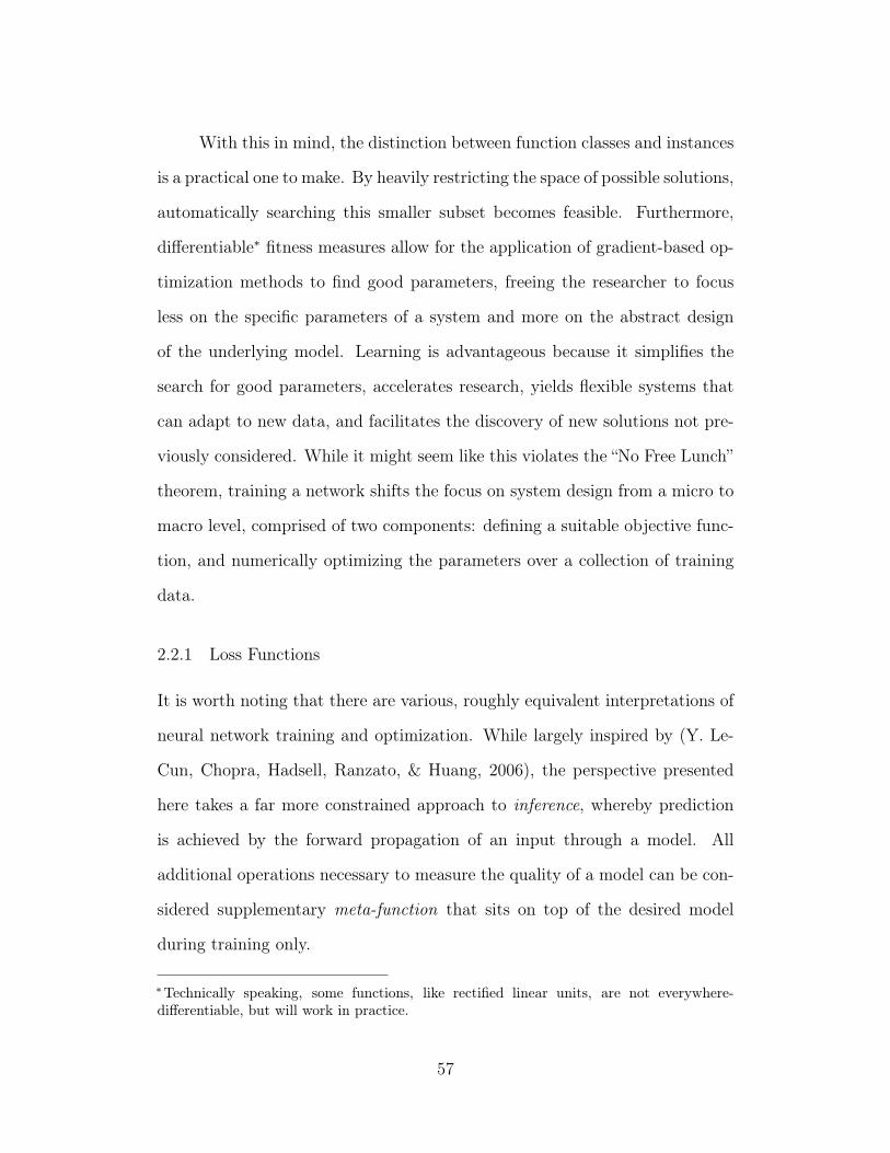
With this in mind, the distinction between function classes and instances
is a practical one to make. By heavily restricting the space of possible solutions,
automatically searching this smaller subset becomes feasible. Furthermore,
differentiable∗ fitness measures allow for the application of gradient-based op-
timization methods to find good parameters, freeing the researcher to focus
less on the specific parameters of a system and more on the abstract design
of the underlying model. Learning is advantageous because it simplifies the
search for good parameters, accelerates research, yields flexible systems that
can adapt to new data, and facilitates the discovery of new solutions not pre-
viously considered. While it might seem like this violates the “No Free Lunch”
theorem, training a network shifts the focus on system design from a micro to
macro level, comprised of two components: defining a suitable objective func-
tion, and numerically optimizing the parameters over a collection of training
data.
2.2.1 Loss Functions
It is worth noting that there are various, roughly equivalent interpretations of
neural network training and optimization. While largely inspired by (Y. Le-
Cun, Chopra, Hadsell, Ranzato, & Huang, 2006), the perspective presented
here takes a far more constrained approach to inference, whereby prediction
is achieved by the forward propagation of an input through a model. All
additional operations necessary to measure the quality of a model can be con-
sidered supplementary meta-function that sits on top of the desired model
during training only.
∗Technically speaking, some functions, like rectified linear units, are not everywhere-differentiable, but will work in practice.
57
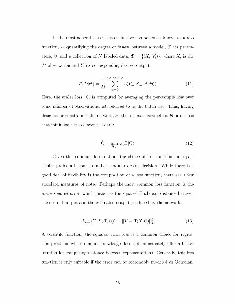
In the most general sense, this evaluative component is known as a loss
function, L, quantifying the degree of fitness between a model, F, its param-
eters, Θ, and a collection of N labeled data, D = {(Xi, Yi)}, where Xi is the
ith observation and Yi its corresponding desired output:
L(D|Θ) =1
M
1≤ M≤ N∑m=0
L(Ym|Xm,F,Θ)) (11)
Here, the scalar loss, L, is computed by averaging the per-sample loss over
some number of observations, M , referred to as the batch size. Thus, having
designed or constrained the network, F, the optimal parameters, Θ, are those
that minimize the loss over the data:
Θ = minΘ∈
L(D|Θ) (12)
Given this common formulation, the choice of loss function for a par-
ticular problem becomes another modular design decision. While there is a
good deal of flexibility is the composition of a loss function, there are a few
standard measures of note. Perhaps the most common loss function is the
mean squared error, which measures the squared Euclidean distance between
the desired output and the estimated output produced by the network:
Lmse(Y |X,F,Θ)) = ||Y − F(X|Θ)||22 (13)
A versatile function, the squared error loss is a common choice for regres-
sion problems where domain knowledge does not immediately offer a better
intution for computing distance between representations. Generally, this loss
function is only suitable if the error can be reasonably modeled as Gaussian.
58
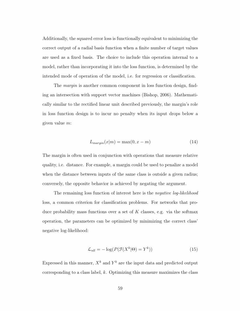
Additionally, the squared error loss is functionally equivalent to minimizing the
correct output of a radial basis function when a finite number of target values
are used as a fixed basis. The choice to include this operation internal to a
model, rather than incorporating it into the loss function, is determined by the
intended mode of operation of the model, i.e. for regression or classification.
The margin is another common component in loss function design, find-
ing an intersection with support vector machines (Bishop, 2006). Mathemati-
cally similar to the rectified linear unit described previously, the margin’s role
in loss function design is to incur no penalty when its input drops below a
given value m:
Lmargin(x|m) = max(0, x−m) (14)
The margin is often used in conjunction with operations that measure relative
quality, i.e. distance. For example, a margin could be used to penalize a model
when the distance between inputs of the same class is outside a given radius;
conversely, the opposite behavior is achieved by negating the argument.
The remaining loss function of interest here is the negative log-likelihood
loss, a common criterion for classification problems. For networks that pro-
duce probability mass functions over a set of K classes, e.g. via the softmax
operation, the parameters can be optimized by minimizing the correct class’
negative log-likelihood:
Lnll = − log(P (F(Xk|Θ) = Y k)) (15)
Expressed in this manner, Xk and Y k are the input data and predicted output
corresponding to a class label, k. Optimizing this measure maximizes the class
59
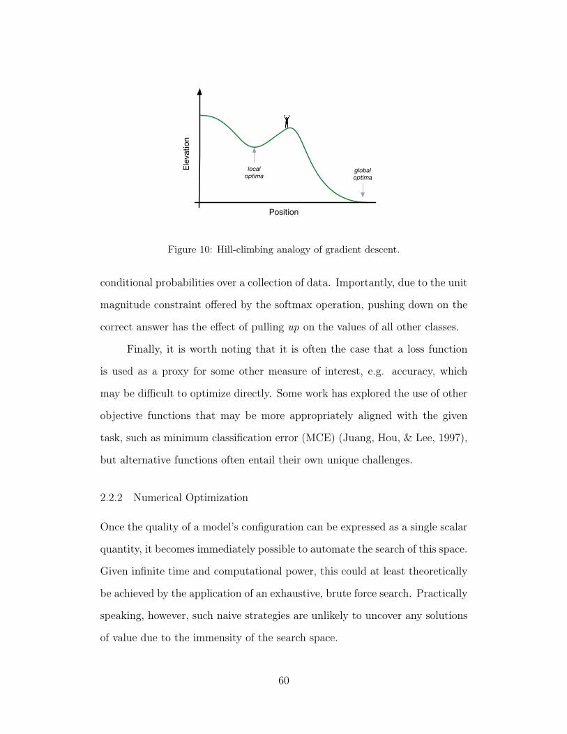
Elev
ation
Position
localoptima
globaloptima
Figure 10: Hill-climbing analogy of gradient descent.
conditional probabilities over a collection of data. Importantly, due to the unit
magnitude constraint offered by the softmax operation, pushing down on the
correct answer has the effect of pulling up on the values of all other classes.
Finally, it is worth noting that it is often the case that a loss function
is used as a proxy for some other measure of interest, e.g. accuracy, which
may be difficult to optimize directly. Some work has explored the use of other
objective functions that may be more appropriately aligned with the given
task, such as minimum classification error (MCE) (Juang, Hou, & Lee, 1997),
but alternative functions often entail their own unique challenges.
2.2.2 Numerical Optimization
Once the quality of a model’s configuration can be expressed as a single scalar
quantity, it becomes immediately possible to automate the search of this space.
Given infinite time and computational power, this could at least theoretically
be achieved by the application of an exhaustive, brute force search. Practically
speaking, however, such naive strategies are unlikely to uncover any solutions
of value due to the immensity of the search space.
60
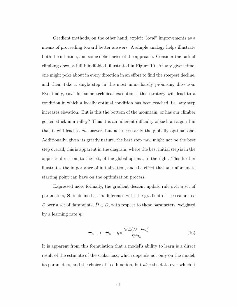
Gradient methods, on the other hand, exploit “local” improvements as a
means of proceeding toward better answers. A simple analogy helps illustrate
both the intuition, and some deficiencies of the approach. Consider the task of
climbing down a hill blindfolded, illustrated in Figure 10. At any given time,
one might poke about in every direction in an effort to find the steepest decline,
and then, take a single step in the most immediately promising direction.
Eventually, save for some technical exceptions, this strategy will lead to a
condition in which a locally optimal condition has been reached, i.e. any step
increases elevation. But is this the bottom of the mountain, or has our climber
gotten stuck in a valley? Thus it is an inherent difficulty of such an algorithm
that it will lead to an answer, but not necessarily the globally optimal one.
Additionally, given its greedy nature, the best step now might not be the best
step overall; this is apparent in the diagram, where the best initial step is in the
opposite direction, to the left, of the global optima, to the right. This further
illustrates the importance of initialization, and the effect that an unfortunate
starting point can have on the optimization process.
Expressed more formally, the gradient descent update rule over a set of
parameters, Θ, is defined as its difference with the gradient of the scalar loss
L over a set of datapoints, D ∈ D, with respect to these parameters, weighted
by a learning rate η:
Θn+1 ← Θn − η ∗∇L(D | Θn)
∇Θn
(16)
It is apparent from this formulation that a model’s ability to learn is a direct
result of the estimate of the scalar loss, which depends not only on the model,
its parameters, and the choice of loss function, but also the data over which it
61
is measured. While early applications of gradient descent for training neural
networks would compute parameter updates using the entire collection of dat-
apoints available for training, deep learning typically leverages batch methods
to approximate the overall loss.
Though the work presented here will focus exclusively on stochastic gra-
dient descent as the numerical optimization method of choice, it is worth
noting that there are alternative methods and extensions one could employ.
In addition to known issues regarding poor local minima, there are also de-
generate cases in which a first-order method like this may be very slow to
converge. In practice however, gradient descent is often sufficient with some
slight modifications, such as the use of slight Nesterov momentum (Sutskever,
Martens, Dahl, & Hinton, 2013). Alternatively, Quasi-Newton methods com-
pute approximations to higher order partial derivatives, which may help the
optimization process recover from problematic regions in the loss surface and
aid in convergence (Liu & Nocedal, 1989). These higher order methods often
entail a higher computational cost, however, and it is not uncommon to em-
ploy them, or their approximations, in tandem with stochastic gradient descent
(Kavukcuoglu et al., 2010).
2.3 Tricks of the Trade
Armed with versatile complex functions and a means to automatically learn
parameters, deep learning seems perfectly posed to tackle a vast array of infor-
mation processing problems. For some time however, however, only a handful
of researchers were able to get positive results, thus earning it its reputation
as a “dark art.” As with many things, the devil is truly in the details, and over
62
time the various tricks and less principled practices necessary for success have
been consolidated into a set of common strategies (Bengio, 2012).
2.3.1 Penalizing Bad Behavior
The goal of architecting a deep network is adjust the representational power of
the model to a given problem, incorporating known constraints where possible.
More often than not, however, a the inherent complexity of a particular model
vastly exceeds the latent complexity of the data at hand. As a result, the
learning process will result in parameter configurations that perform well on
the training data, but fail to generalize to unseen data. Conceptually, this
can be understood as the model having too many options when achieving its
goal state, and happening to pick one that is bad for reasons that do not
factor into its objective function. It can be said that the learning problem is
under-determined, and thus additional penalties can be added to the overall
loss. Interestingly enough, this penalty-based approach is common practice
in other greedy optimization systems, like capitalistic markets, where taxes
and fines serve to discourage certain outcomes, e.g. dumping industrial by-
products in a river.
While it is conceivable that any number of undesirable system behaviors
could be quantified by some scalar measure, there are two general approaches
common across deep learning. The first, referred to as weight decay, ridge
regression, or L2-regularization, is classic across machine learning, and finds
use in a variety of learning algorithms:
Ldecay =∑i
λ ||Θi||22 (17)
63
Here, the vector magnitude of the ith parameter, Θi, is weighted by a
hyperparameter, λi, and summed together as a scalar penalty. Convention-
ally, the same weight is applied to all parameters, although differently shaped
parameters will bias the cumulative term. During optimization, this has the
effect of driving parameters toward, but not exactly, zero, providing an intu-
itive interpretation consistent with Occam’s razor, i.e. prefer simpler solutions.
This often prevents the network from overfitting the training data exactly, and
resulting in solutions that generalize better.
Whereas weight decay is applied to the parameters of network, sparsity
penalties are applied over intermediary representations in a network, taking
the form of a cumulative weighted vector magnitude in L1 space:
Lsparsity =∑i
λ ||Zi||1 (18)
Ideally, it would be more preferable to optimize the L0 loss. This this problem
is generally np-hard, however, and the L1 loss, its convex envelope, serves as
a differentiable approximation. While it is not guaranteed that the solutions
of each may coincide, optimizing the L1 generally yields good results in prac-
tice. As a result, this penalty will prefer sparse representations, which help
disentangle factors of variation in the data (Bengio, 2009).
2.3.2 Parameter Initialization
As shown previously in the discussion of gradient descent, poor initial condi-
tions can delay, or in some cases even prevent, an optimization algorithm
from finding good solutions. Attempts to train deep networks with error
back-propagation can compound this issue, as an error signal can become
64
insignificantly small after several layers under certain conditions. While this
is somewhat sensitive to the architectural decisions made, such as the choice
of non-linearities used, all networks are sensitive to parameter initialization.
In general, sampling coefficients from appropriately tuned random dis-
tributions leads to reasonably good results. There is little consensus on the
advantages of a uniform versus normal distribution for initialization, but the
primary factor to control in either case is the dynamic range or scale. As a
rule of thumb, this can be automated somewhat by using the fan-in, or dimen-
sionality of the input, to keep the activations of within the operating region
of saturating transfer functions, i.e. sigmoid or hyperbolic tanget. Rectified
linear units, on the other hand, are far less sensitive to the choice of initializa-
tion, as half of its operating region is non-saturating, contributing to their rise
in popularity. As a result, sufficiently small, centered normal distributions,
N(µ = 0, σ ≈ 0.01), work well in practice.
Alternatively, unsupervised pre-training methods, credited with effec-
tively jump-starting the rennaisance of deep learning, can be used to initialize
networks in a data-driven manner. Though there are different perspectives on
how this can be achieved, the core concept is the same: using a large amount
of unlabeled data, train a deep network to reconstruct realistic observations
in a greedy, layer-wise manner. Then, once all layers have been initialized,
conventional supervised training can be applied. In theory, this data-driven
process works by getting the parameters of the network closer to a good solu-
tion. As mentioned previously, the first successful realization of this idea used
restricted Boltzmann machines (RBMs) (G. E. Hinton et al., 2006), leveraging
Gibbs sampling and contrastive divergence to produce realistic samples from
the model. The deterministic variant is the autoencoder, which use data aug-
65
mentation, sparsity, or weight tying to train a pair of deep, invertible functions
(Bengio, Courville, & Vincent, 2013). Most recently, unsupervised pre-training
has fallen out of favor somewhat, as comparable results can be obtained with
rectified linear units and randomized weights, provided there is sufficient la-
beled data. That said, this strategy may still prove useful for problems in
which it is difficult to obtain a large amount of labeled information, such as
personalized systems.
2.3.3 Dropout
Another recent addition to canon of deep learning practicum is the training
strategy known as dropout (G. E. Hinton, Srivastava, Krizhevsky, Sutskever, &
Salakhutdinov, 2012). As the name suggests, some percentage of parameters
in a network are randomly “dropped” during training in estimating the loss
and computing an update step. The details of how exactly this is done vary
slightly from sub-function to sub-function, but a description in terms of an
affine transformation is sufficiently illustrative:
Z = f(Z|p) =1
(1− p)ZB(1, p)M
Here, the activations of an affine transformation, Z, a column vector of length
M , are masked by a Bernoulli distribution, B, with probability p. To offset
the effect of smaller magnitudes resulting from fewer units being active during
training, these outputs are scaled by one minus the probability parameter,
such that, in expectation over B, the use of dropout matches the original
function. Applied in this manner, this prevents rows, or bases, in the matrix
66
projection from contributing to the final output, inhibiting the co-adaptation
of parameters. Thus dropout is effective because the parameters are unable
to depend on one another for effectiveness, and tend to learn independently
good features.
Additionally, dropout has an interesting relationship with model aver-
aging, or bagging. Masking parameters has the effect of selecting a subset of
parameters from the given model, and therefore one of many complementary
models is updated at each training iteration. This reduces the theoretical
bound on generalization error, and has been proven to greatly improve results
for models prone to overfitting.
2.3.4 Data Augmentation
A common strategy among deep learning practitioners is to leverage domain
knowledge wherever possible. While this has an obvious connection to the
architectural design and choice of loss function, another oft exploited, though
less documented, opportunity is through the application of data augmentation.
The main idea here is that a collection of labeled data can be manipulated
in varying degrees of realism. This exploits the common scenario that model-
ing the synthesis process is typically easier than the analysis process. While
the most effective distortions are rather domain specific, common deformations
include operations such as translation, scaling, additive noise, nonlinear distor-
tion. In this space of music, this could range from signal-level attributes, like
perceptual codecs or production effects, to musically inspired augmentations,
such as pitch shifting or time-stretching.
67
2.3.5 Normalization
Finally, enough cannot be said about the importance of proper data normal-
ization. The simplest form of data normalization is maximum scaling, such
that all datapoints are bounded on the same input region. Another form of dy-
namic range control is achieved by normalizing inputs to have unit magnitude
in some Lp-space, e.g. Euclidean. Alternatively, coefficient-wise standardiza-
tion is strongly advocated, e.g. subtract the mean and divide by standard
deviation. This can be extended via principal components analysis (PCA),
which offers the added benefit of dimensionality reduction, or PCA-whitening
(alternatively, ZCA), which “whitens” the data by scaling coefficients by their
eigenvalues. Lastly, local contrast normalization (LCN) has proven to be a
particularly useful approach to data normalization (Sermanet, Kavukcuoglu,
Chintala, & LeCun, 2013). Finding inspiration from biological processes, LCN
performs a form of automatic gain control over local neighborhoods, and can
lead to surprisingly discriminative features even in the absence of training
(Kavukcuoglu et al., 2010).
In addition to constraining the input space, it is also common to con-
strain the parameters within a network, often taking two forms. In some
cases, like (G. E. Hinton et al., 2012), parameters are simply constrained in-
side the volume of the given hypersphere, such that any time parameters are
updated to values that result in a magnitude larger than 1, they are rescaled.
This constraint gives parameters freedom to adapt to the nuances of the data
without growing arbitrarily large to offset the contributions of small weights.
Bounding parameters shares a loose connection to weight decay, in parameters
are prevented from growing arbitrarily large, without the need for additional
68
penalties or hyperparameters. Alternatively, there are also successful instances
of weights being constrained to the surface of the L2 hypersphere, a common
approach in various forms of sparse coding.
3 Summary
Building upon formal logic and biological analogy, neural networks were de-
vised in the 1960s as an approach to information processing. However, after
initial promise, they were largely met with skepticism, indifference, or worse
through the remainder of the century. The few who persevered made vari-
ous discoveries that, coupled with steady advances in computing technology,
would eventually return neural computation to the fore: mini-batch stochastic
gradient descent made optimization computationally efficient and less suscep-
tible to poor local minima, and encouraged further exploration of numerical
optimization methods; convolutional networks reduced model complexity and
over-fitting through scale and translation invariance; and lastly, larger labeled
datasets reduced overfitting, and abundant unlabeled data could be used to
better initialize networks in an unsupervised manner.
Deep learning is therefore based on two principles: first, that complex
problems can be decomposed into a series of simpler subproblems; and second,
what exactly these simpler subproblems are or should be can be discovered
from a corpus of data.
69
CHAPTER IV
TIMBRE SIMILARITY
Timbre has proven to be a difficult attribute to define in acoustic percep-
tion, and there is little concensus as result in its underpinnings or the efforts
to model it computationally. Psychoacoustics has long sought to better under-
stand the space of timbre using subjective pairwise ratings between acoustic
stimuli, but this information is costly to obtain and the generalizability of
conclusions ultimately dependent on the palette of sounds considered. This
chapter explores an objective, data-driven approach to the development of
relative timbre spaces as a scalable alternative to this line of research. Here,
instrument taxonomies are used to as a proxy for timbre similarity, and a
deep convolutional network is used to project time-frequency representations
of audio into a low-dimensional, semantically organized space. The quality
of the resulting embeddings is demonstrated through a series of experiments,
indicating that this approach shows significant promise for organizing large
collections of audio samples by timbre.
1 Context
Despite its common usage in the various forms of music for centuries, a satis-
factory definition of timbre remains elusive to this day; in fact, the one adopted
by the American National Standards Institute embodies this challenge, arriv-
ing at a concept through the exclusion of others (Sonn, Martin, 1973):
70
Timbre is that attribute of auditory sensation in terms of which a
subject can judge that two sounds similarly presented and having
the same loudness and pitch are dissimilar.
As evidenced by this definition, the very notion of “timbre” is still an open
research topic in psychoacoustics. This reality is captured quite succinctly
by Phillipe Manoury, who offered the following insight (Manoury, 1991), as
translated by (Donnadieu, 2007):
One of the most striking paradoxes concerning timbre is that when
we knew less about it, it didn’t pose much of a problem.
There are many advantages to developing a deeper understanding of
timbre, from both an artistic and scientific perspective. Of particular interest
to this work, however, the absence of a constructive definition —timbre is
a result of X, Y, and Z— makes it difficult to directly build computational
systems to characterize and compare timbres. Thus, before proceeding, it is
valuable to review what is known of timbre, and prior efforts to transfer this
knowledge into engineering systems.
1.1 Psychoacoustics
The perception of timbre falls under the umbrella of psychoacoustics, a topic
of study that sits at the boundary between acoustics and psychology. Some of
the earliest research in psychoacoustics was pioneered by von Helmholtz in his
inquiries into the sensations of pitch and loudness (Bregman, 1994). Inquiries
specific to timbre would not come until much later, due to two difficulties
in experimental design. One, whereas pitch and loudness can be ranked on
71
a one dimensional scale, it is unclear from personal introspection what the
salient dimensions of timbre might be. Instead, it is often necessary to use
metaphors as a means of comparing and relating the perception of timbre,
such as describing a sound as “bright” or “muddy”. Additionally, researchers
were limited by the kinds of stimuli they could create and use in perceptual
experimentation, and thus were constrained in the space of possible parameters
to explore.
With the advent of computers and continued scientific advances through
the 20th century, these issues could be addressed directly, and several re-
searchers set out to identify the existence of fundamental dimensions. This
work, performed by Plomp (Plomp, 1976) and Grey (Grey, 1977), among oth-
ers, adopted a similar experimental design. Human subjects are presented
pairs of sound stimuli and asked to rate the similarity between the two. Hav-
ing collected an exhaustive set of pairwise ratings from a number of partic-
ipants, multi-dimensional scaling is then used to project the stimuli into a
low-dimensional space such that the reported relationships between these dat-
apoints are minimally distorted (Grey, 1977); an example space is shown in
Figure 11. Using this similarity model, the researcher then considers a wide
array of time-frequency signal statistics, or features, in order to identify those
that best correlate with the different dimensions. This approach has produced
a useful, albeit large, set of features on which computational models have been
constructed. Among the earliest were those of log-attack time, spectral cen-
troid, and spectral spread, and were later corroborated by other researchers,
as in the work of (McAdams, Winsberg, Donnadieu, De Soete, & Krimphoff,
1995).
More recently, however, some have begun to recognize a few shortcom-
72
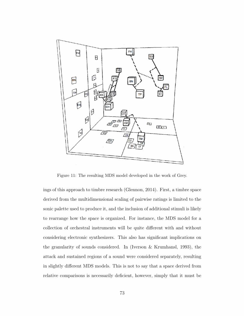
Figure 11: The resulting MDS model developed in the work of Grey.
ings of this approach to timbre research (Glennon, 2014). First, a timbre space
derived from the multidimensional scaling of pairwise ratings is limited to the
sonic palette used to produce it, and the inclusion of additional stimuli is likely
to rearrange how the space is organized. For instance, the MDS model for a
collection of orchestral instruments will be quite different with and without
considering electronic synthesizers. This also has significant implications on
the granularity of sounds considered. In (Iverson & Krumhansl, 1993), the
attack and sustained regions of a sound were considered separately, resulting
in slightly different MDS models. This is not to say that a space derived from
relative comparisons is necessarily deficient, however, simply that it must be
73
adapted in the presence of new or different information. Second, the process
of finding well-correlated features to explain the resulting MDS model is dif-
ficult and time consuming. A researcher must repeat the involved process of
feature exploration for every model obtained through a different combination
of stimuli. Furthermore, as noted by Caclin et al., “Given the multiplicity
of acoustical parameters that could be proposed to explain perceptual dimen-
sions, one can never be sure that the selected parameters do not merely covary
with the true underlying parameters.” (Caclin, McAdams, Smith, &Winsberg,
2005). In other words, correlation does not imply causation, and features iden-
tified by inspection entail some degree of uncertainty. Finally, the process of
collecting subjective pairwise ratings is especially costly, because the number
of possible comparisons increases quadratically with number of unique stimuli
considered. This places a practical constraint on the generality of a timbre
space, as it quickly becomes impossible for subjects to exhaustively rate all
combinations. In the absence of complete information, statistical methods,
such as imputation, are necessary to interpolate a sparse set of responses.
1.2 Computational Modeling of Timbre
Most previous approaches to computationally modeling timbre instantaneously
can be grouped into one of two categories: signal statistics and basis projec-
tions. The first follows from the perceptual research described above, whereby
specific features are designed to encode some high level semantic concept, e.g.
log-attack time or spectral brightness. Initially these corresponded to the fea-
tures named by in the work of Grey or Krumhansl, but have expanded over
time to include a wide array of creative and clever measures. The interested
74
reader is directed to (Essid, Richard, & David, 2006) for a comprehensive space
of possible features.
From an often complementary perspective, other music researchers have
utilised transform-based approaches to project signals into representations
with various desirable properties. One of the earliest and most common ap-
proaches is the use of Mel-frequency Cepstral Coefficients (MFCCs) for timbre-
oriented tasks. Originally designed for speech coding in the 1980s (Davis &
Mermelstein, 1980), the first significant contribution in MIR to call atten-
tion to MFCCs as useful music features was that of Logan in 2000 (Logan,
2000). MFCCs have, at least in practice, become nearly synonymous with
timbre-centric MIR, now being used in a wide array of systems for instrument
classification (Herrera-Boyer, Peeters, & Dubnov, 2003), tagging (Barrington,
Yazdani, Turnbull, & Lanckriet, 2008), genre prediction (Tzanetakis & Cook,
2002), mood estimation (Schmidt & Kim, 2010) or structural analysis (Paulus,
Müller, & Klapuri, 2010), to name only a few works. As described in detail
in Chapter II, the general process of computing MFCCs proceeds as follows:
an input audio signal is divided into overlapping, short-time frames, on the
order of tens to hundreds of milliseconds; a filterbank, perceptually scaled
in frequency, is then applied to each short-time frame and log-compressed;
finally, a discrete cosine transform (DCT) is applied to these frequency co-
efficients, characterizing the shape of the spectrum (or the spectrum of the
spectrum, referred to as the cepstrum). Only the first dozen or so coefficients
are used, based on the principle that they compactly describe the spectral
contour, though this is more convention than rule. Some have even gone so far
as to literally equate MFCCs and timbre, concluding that specific coefficients
75
are responsible for various perceptual dimensions (Terasawa, Slaney, & Berger,
2005).
Similar in principle, though less widely adopted, is to instead learn the
set of bases against which a time-frequency representation is projected. One
such instance is observed in (Jehan, 2005), which preserves the first 12 coef-
ficients of a trained PCA decomposition. In this scenario, the projection into
the PCA subspace serves to decorrelate the principal axes of the data in the
input space, much like the Discrete Cosine Transform. The primary difference
here, however, is that the bases are learned from a sample of observations,
rather than defined analytically.
1.3 Motivation
While many computational approaches have proven useful for various classifi-
cation or recognition tasks, none directly result in a notion of timbre similarity,
a useful concept with a variety of applications. One notable instance is the
difficulty faced in the search and navigation of large sound sample libraries.
Queries are predominantly forced to take the form of text, as in the Freesound∗
archive shown in Figure 12, which is problematic for at least two reasons. On
one hand, it can challenging to describe a specific query semantically, and of-
ten metaphors and figurative language are used to relate the experience of a
sound; a distorted guitar might be referred to as ‘crunchy’, or a trumpet as
‘bright.’ Conversely, this kind of descriptive language is far from standardized
and varies in meaning from one individual to the next. Furthermore, such
descriptions are not always associated with every sound in a collection, and
∗http://www.freesound.org/
76
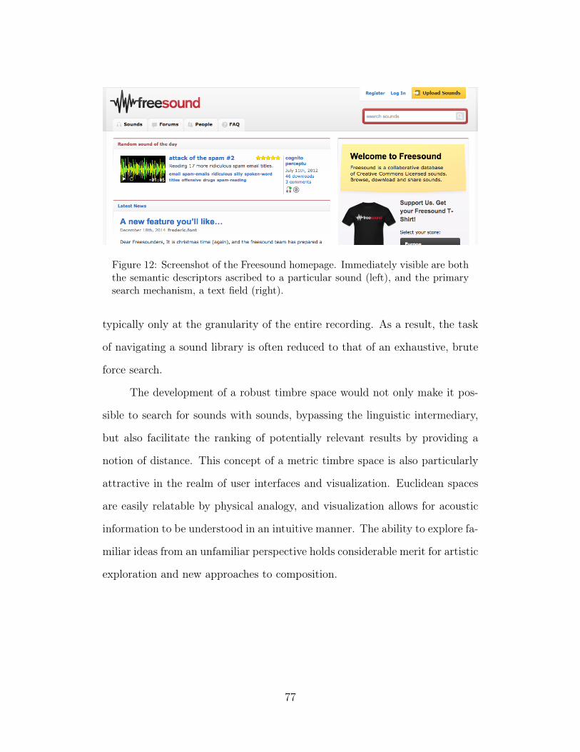
Figure 12: Screenshot of the Freesound homepage. Immediately visible are boththe semantic descriptors ascribed to a particular sound (left), and the primarysearch mechanism, a text field (right).
typically only at the granularity of the entire recording. As a result, the task
of navigating a sound library is often reduced to that of an exhaustive, brute
force search.
The development of a robust timbre space would not only make it pos-
sible to search for sounds with sounds, bypassing the linguistic intermediary,
but also facilitate the ranking of potentially relevant results by providing a
notion of distance. This concept of a metric timbre space is also particularly
attractive in the realm of user interfaces and visualization. Euclidean spaces
are easily relatable by physical analogy, and visualization allows for acoustic
information to be understood in an intuitive manner. The ability to explore fa-
miliar ideas from an unfamiliar perspective holds considerable merit for artistic
exploration and new approaches to composition.
77
1.4 Limitations
It is valuable to note that despite the difficulty inherent to defining timbre,
all computational research must adopt some working concept of it, implicitly
or otherwise. Generally two facets to timbre; sound quality and sound source.
They are related but not exactly equal. The work presented here operates on
the assumption that the perception of timbre is tightly coupled with the expe-
rience of discriminating between unique sound sources. This is not intended
to be a true equivalence with timbre, but a functional approximation that al-
lows the research to proceed. Compromise and simplification; You’ll pay out
somewhere. Human judgments of similarity absolve you assumptions about
the relationship between source and quality, but costly to curate at scale. A
data-driven approach, on the other hand, offers the opposite scenario; it is
relatively simple to collect this data, but requires that assumptions be made
regarding the quality being related.
Ensemble versus solo. Here focus entirely on the latter.
2 Learning Timbre Similarity
From the previous review of psychoacoustics research and efforts to computa-
tionally explain timbre, there is an important series of observations to consider.
Classic timbre features are discovered through an involved process of design-
ing a number of signal-level statistics and identifying which correlate with the
dimensions of a model. Importantly, those statistics that best explain a timbre
space are only valid in the context of the sound sources considered, and thus
the process should be repeated for different sonic palettes. Additionally, the
subjective ratings necessary to conduct this kind of research are costly to ob-
78
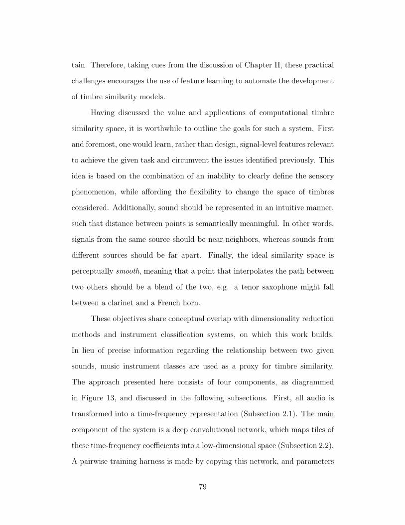
tain. Therefore, taking cues from the discussion of Chapter II, these practical
challenges encourages the use of feature learning to automate the development
of timbre similarity models.
Having discussed the value and applications of computational timbre
similarity space, it is worthwhile to outline the goals for such a system. First
and foremost, one would learn, rather than design, signal-level features relevant
to achieve the given task and circumvent the issues identified previously. This
idea is based on the combination of an inability to clearly define the sensory
phenomenon, while affording the flexibility to change the space of timbres
considered. Additionally, sound should be represented in an intuitive manner,
such that distance between points is semantically meaningful. In other words,
signals from the same source should be near-neighbors, whereas sounds from
different sources should be far apart. Finally, the ideal similarity space is
perceptually smooth, meaning that a point that interpolates the path between
two others should be a blend of the two, e.g. a tenor saxophone might fall
between a clarinet and a French horn.
These objectives share conceptual overlap with dimensionality reduction
methods and instrument classification systems, on which this work builds.
In lieu of precise information regarding the relationship between two given
sounds, music instrument classes are used as a proxy for timbre similarity.
The approach presented here consists of four components, as diagrammed
in Figure 13, and discussed in the following subsections. First, all audio is
transformed into a time-frequency representation (Subsection 2.1). The main
component of the system is a deep convolutional network, which maps tiles of
these time-frequency coefficients into a low-dimensional space (Subsection 2.2).
A pairwise training harness is made by copying this network, and parameters
79
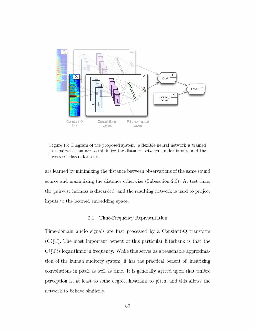
fifj
Z2X2
Constant-QTFR
ConvolutionalLayers
Fully-connectedLayers
fifj
Cost
Loss
SimilarityScore
X1Z1
D
Y
L
Figure 13: Diagram of the proposed system: a flexible neural network is trainedin a pairwise manner to minimize the distance between similar inputs, and theinverse of dissimilar ones.
are learned by minimizing the distance between observations of the same sound
source and maximizing the distance otherwise (Subsection 2.3). At test time,
the pairwise harness is discarded, and the resulting network is used to project
inputs to the learned embedding space.
2.1 Time-Frequency Representation
Time-domain audio signals are first processed by a Constant-Q transform
(CQT). The most important benefit of this particular filterbank is that the
CQT is logarithmic in frequency. While this serves as a reasonable approxima-
tion of the human auditory system, it has the practical benefit of linearizing
convolutions in pitch as well as time. It is generally agreed upon that timbre
perception is, at least to some degree, invariant to pitch, and this allows the
network to behave similarly.
80
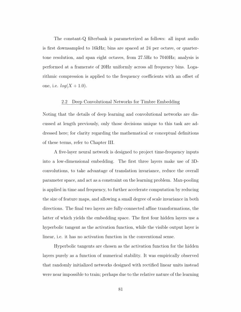
The constant-Q filterbank is parameterized as follows: all input audio
is first downsampled to 16kHz; bins are spaced at 24 per octave, or quarter-
tone resolution, and span eight octaves, from 27.5Hz to 7040Hz; analysis is
performed at a framerate of 20Hz uniformly across all frequency bins. Loga-
rithmic compression is applied to the frequency coefficients with an offset of
one, i.e. log(X + 1.0).
2.2 Deep Convolutional Networks for Timbre Embedding
Noting that the details of deep learning and convolutional networks are dis-
cussed at length previously, only those decisions unique to this task are ad-
dressed here; for clarity regarding the mathematical or conceptual definitions
of these terms, refer to Chapter III.
A five-layer neural network is designed to project time-frequency inputs
into a low-dimensional embedding. The first three layers make use of 3D-
convolutions, to take advantage of translation invariance, reduce the overall
parameter space, and act as a constraint on the learning problem. Max-pooling
is applied in time and frequency, to further accelerate computation by reducing
the size of feature maps, and allowing a small degree of scale invariance in both
directions. The final two layers are fully-connected affine transformations, the
latter of which yields the embedding space. The first four hidden layers use a
hyperbolic tangent as the activation function, while the visible output layer is
linear, i.e. it has no activation function in the conventional sense.
Hyperbolic tangents are chosen as the activation function for the hidden
layers purely as a function of numerical stability. It was empirically observed
that randomly initialized networks designed with rectified linear units instead
were near impossible to train; perhaps due to the relative nature of the learning
81
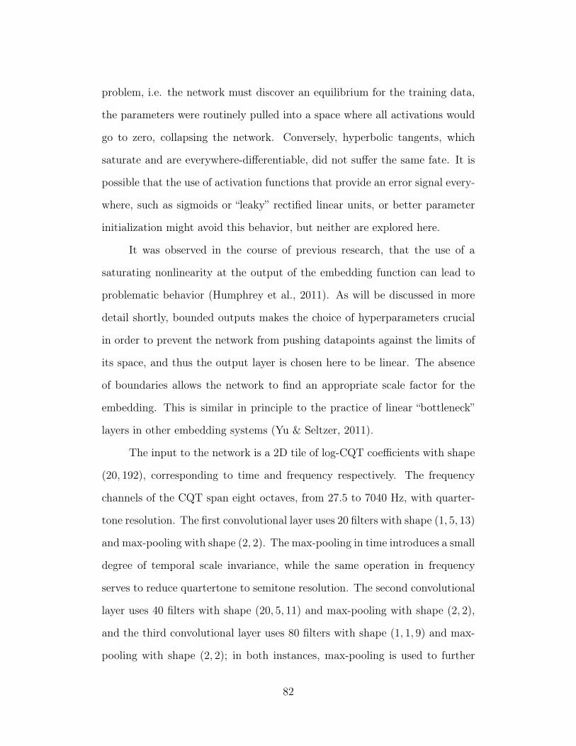
problem, i.e. the network must discover an equilibrium for the training data,
the parameters were routinely pulled into a space where all activations would
go to zero, collapsing the network. Conversely, hyperbolic tangents, which
saturate and are everywhere-differentiable, did not suffer the same fate. It is
possible that the use of activation functions that provide an error signal every-
where, such as sigmoids or “leaky” rectified linear units, or better parameter
initialization might avoid this behavior, but neither are explored here.
It was observed in the course of previous research, that the use of a
saturating nonlinearity at the output of the embedding function can lead to
problematic behavior (Humphrey et al., 2011). As will be discussed in more
detail shortly, bounded outputs makes the choice of hyperparameters crucial
in order to prevent the network from pushing datapoints against the limits of
its space, and thus the output layer is chosen here to be linear. The absence
of boundaries allows the network to find an appropriate scale factor for the
embedding. This is similar in principle to the practice of linear “bottleneck”
layers in other embedding systems (Yu & Seltzer, 2011).
The input to the network is a 2D tile of log-CQT coefficients with shape
(20, 192), corresponding to time and frequency respectively. The frequency
channels of the CQT span eight octaves, from 27.5 to 7040 Hz, with quarter-
tone resolution. The first convolutional layer uses 20 filters with shape (1, 5, 13)
and max-pooling with shape (2, 2). The max-pooling in time introduces a small
degree of temporal scale invariance, while the same operation in frequency
serves to reduce quartertone to semitone resolution. The second convolutional
layer uses 40 filters with shape (20, 5, 11) and max-pooling with shape (2, 2),
and the third convolutional layer uses 80 filters with shape (1, 1, 9) and max-
pooling with shape (2, 2); in both instances, max-pooling is used to further
82
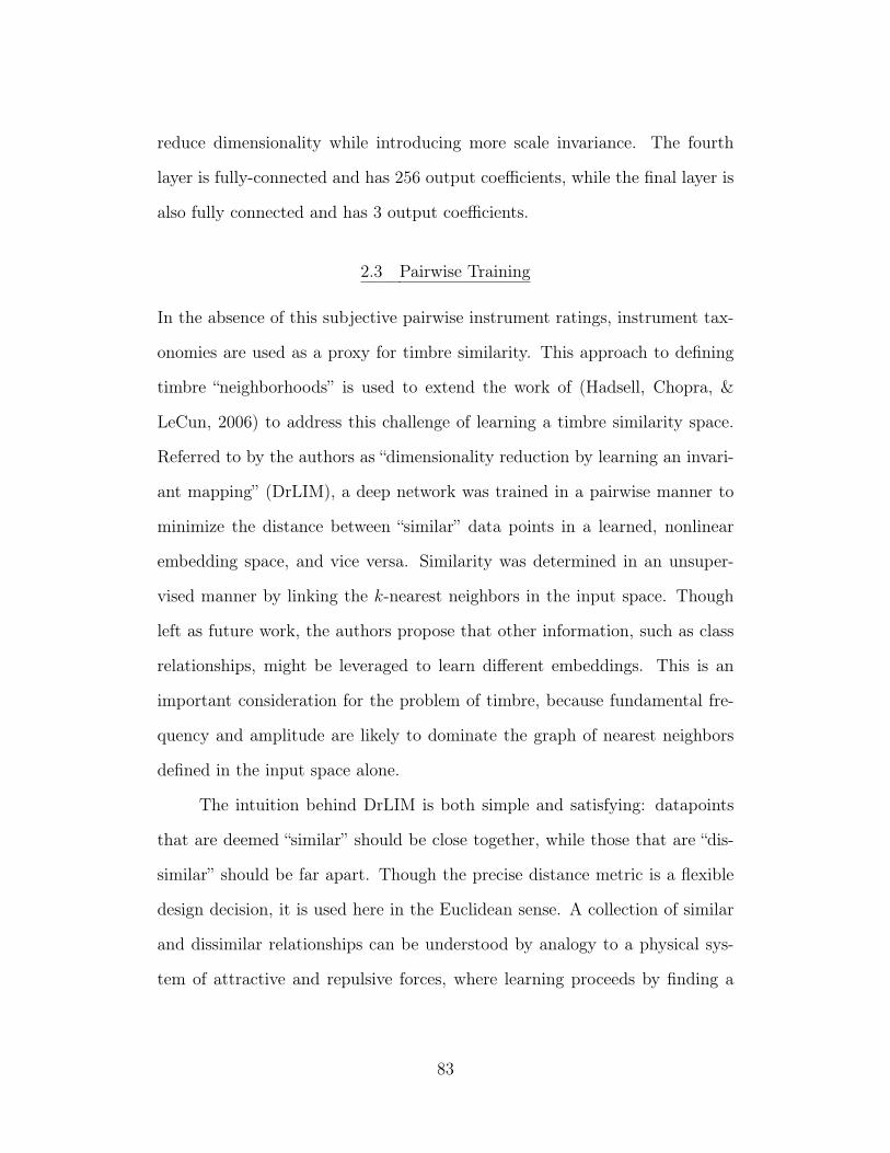
reduce dimensionality while introducing more scale invariance. The fourth
layer is fully-connected and has 256 output coefficients, while the final layer is
also fully connected and has 3 output coefficients.
2.3 Pairwise Training
In the absence of this subjective pairwise instrument ratings, instrument tax-
onomies are used as a proxy for timbre similarity. This approach to defining
timbre “neighborhoods” is used to extend the work of (Hadsell, Chopra, &
LeCun, 2006) to address this challenge of learning a timbre similarity space.
Referred to by the authors as “dimensionality reduction by learning an invari-
ant mapping” (DrLIM), a deep network was trained in a pairwise manner to
minimize the distance between “similar” data points in a learned, nonlinear
embedding space, and vice versa. Similarity was determined in an unsuper-
vised manner by linking the k-nearest neighbors in the input space. Though
left as future work, the authors propose that other information, such as class
relationships, might be leveraged to learn different embeddings. This is an
important consideration for the problem of timbre, because fundamental fre-
quency and amplitude are likely to dominate the graph of nearest neighbors
defined in the input space alone.
The intuition behind DrLIM is both simple and satisfying: datapoints
that are deemed “similar” should be close together, while those that are “dis-
similar” should be far apart. Though the precise distance metric is a flexible
design decision, it is used here in the Euclidean sense. A collection of similar
and dissimilar relationships can be understood by analogy to a physical sys-
tem of attractive and repulsive forces, where learning proceeds by finding a
83
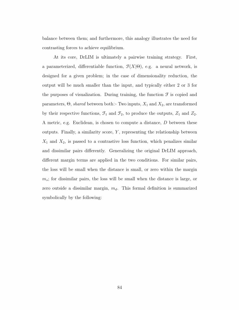
balance between them; and furthermore, this analogy illustrates the need for
contrasting forces to achieve equilibrium.
At its core, DrLIM is ultimately a pairwise training strategy. First,
a parameterized, differentiable function, F(X|Θ), e.g. a neural network, is
designed for a given problem; in the case of dimensionality reduction, the
output will be much smaller than the input, and typically either 2 or 3 for
the purposes of visualization. During training, the function F is copied and
parameters, Θ, shared between both> Two inputs, X1 andX2, are transformed
by their respective functions, F1 and F2, to produce the outputs, Z1 and Z2.
A metric, e.g. Euclidean, is chosen to compute a distance, D between these
outputs. Finally, a similarity score, Y , representing the relationship between
X1 and X2, is passed to a contrastive loss function, which penalizes similar
and dissimilar pairs differently. Generalizing the original DrLIM approach,
different margin terms are applied in the two conditions. For similar pairs,
the loss will be small when the distance is small, or zero within the margin
ms; for dissimilar pairs, the loss will be small when the distance is large, or
zero outside a dissimilar margin, md. This formal definition is summarized
symbolically by the following:
84
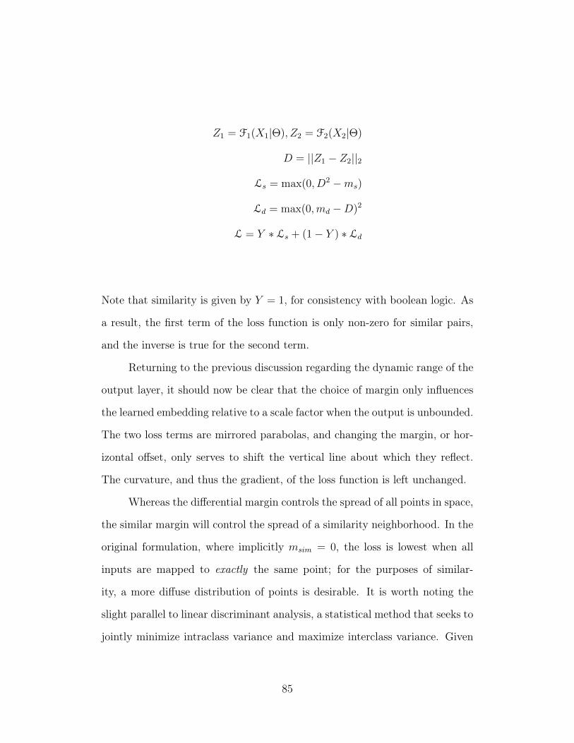
Z1 = F1(X1|Θ), Z2 = F2(X2|Θ)
D = ||Z1 − Z2||2
Ls = max(0, D2 −ms)
Ld = max(0,md −D)2
L = Y ∗ Ls + (1− Y ) ∗ Ld
Note that similarity is given by Y = 1, for consistency with boolean logic. As
a result, the first term of the loss function is only non-zero for similar pairs,
and the inverse is true for the second term.
Returning to the previous discussion regarding the dynamic range of the
output layer, it should now be clear that the choice of margin only influences
the learned embedding relative to a scale factor when the output is unbounded.
The two loss terms are mirrored parabolas, and changing the margin, or hor-
izontal offset, only serves to shift the vertical line about which they reflect.
The curvature, and thus the gradient, of the loss function is left unchanged.
Whereas the differential margin controls the spread of all points in space,
the similar margin will control the spread of a similarity neighborhood. In the
original formulation, where implicitly msim = 0, the loss is lowest when all
inputs are mapped to exactly the same point; for the purposes of similar-
ity, a more diffuse distribution of points is desirable. It is worth noting the
slight parallel to linear discriminant analysis, a statistical method that seeks to
jointly minimize intraclass variance and maximize interclass variance. Given
85
the relative nature of this trade-off, it is sufficient to pick a single ratio between
the margins, eliminating the need to vary both hyperparameters separately.
In practice, training proceeded via minibatch stochastic gradient descent
with a constant learning rate, set at 0.02 for 25k iterations, or until a batch
returned a total loss of zero. Batches consisted of 100 comparisons, drawn
such that a datapoint was paired with both a positive and negative example.
3 Methodology
To assess the viability of data-driven nonlinear semantic embeddings for timbre
similarity, and thus address the goals outlined at the outset of Section 2, two
experiments are used to quantify different performance criteria. First, the
local structure and class boundaries of the learned embeddings are explored
with a classification task. Second, global organization of the space is measured
by a ranked retrieval task. Additionally, in lieu of a subjective evaluation of
perceptual “smoothness” of the resulting timbre space, the learned embeddings
are investigated through confusion analysis and visualization. In each instance,
the approach presented here is compared to a conceptually similar, albeit
admittedly simpler, system.
Finally, the formulation described in the previous section presents two
system variables, thus giving rise to two additional considerations:
1. What is the effect of using different margin ratios?
2. How does the sonic palette considered impact the learned embedding?
86
3.1 Data
The data source used herein is drawn from the Vienna Symphonic Library
(VSL), a truly massive collection of studio-grade orchestral instrument samples
recorded over a variety of performance techniques∗. In aggregate, the VSL
contains over 400k sound recordings from more than 40 different instruments,
both pitched and percussive. Sorting instrument classes by sample count yields
27 instruments with at least 5k samples; three of these instruments, however,
are not reasonably distinct from other sources, e.g. “flute-1” and “flute-2”, and
discarded rather than risk introducing conflicting information. This decision
yields the set of instruments contained in Table 1 for experimentation.
The distribution of sound files for these instruments, grouped by class,
is given in Figure 14. As discussed previously, it is an inherent difficulty of
pairwise similarity models that the resulting relationships are limited by the
number of unique classes considered. Fortunately, there is no added cost to
considering a wider palette of sound sources here because the label information
is objective. Therefore, building upon previous work (Humphrey et al., 2011),
three configuration subsets are repeated from the pilot study as well as a fourth
consisting of all 24 classes, given in Table 2.
For each instrument class, 5k samples are drawn, without replacement, to
build a uniformly distributed collection. This step simplifies the process of data
sampling during stochastic training of the network, which may be sensitive
to class imbalances. The collection of instrument samples is stratified into
five equal partitions for cross validation, used at a ratio of 3-1-1 for training,
∗https://vsl.co.at/en
87
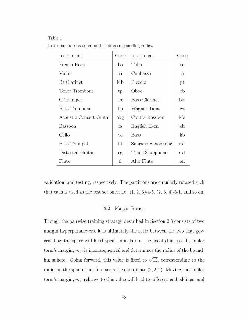
Table 1
Instruments considered and their corresponding codes.
Instrument Code Instrument Code
French Horn ho Tuba tu
Violin vi Cimbasso ci
B[ Clarinet klb Piccolo pt
Tenor Trombone tp Oboe ob
C Trumpet trc Bass Clarinet bkl
Bass Trombone bp Wagner Tuba wt
Acoustic Concert Guitar akg Contra Bassoon kfa
Bassoon fa English Horn eh
Cello vc Bass kb
Bass Trumpet bt Soprano Saxophone sxs
Distorted Guitar eg Tenor Saxophone sxt
Flute fl Alto Flute afl
validation, and testing, respectively. The partitions are circularly rotated such
that each is used as the test set once, i.e. (1, 2, 3)-4-5, (2, 3, 4)-5-1, and so on.
3.2 Margin Ratios
Though the pairwise training strategy described in Section 2.3 consists of two
margin hyperparameters, it is ultimately the ratio between the two that gov-
erns how the space will be shaped. In isolation, the exact choice of dissimilar
term’s margin, md, is inconsequential and determines the radius of the bound-
ing sphere. Going forward, this value is fixed to√
12, corresponding to the
radius of the sphere that intersects the coordinate (2, 2, 2). Moving the similar
term’s margin, ms, relative to this value will lead to different embeddings, and
88
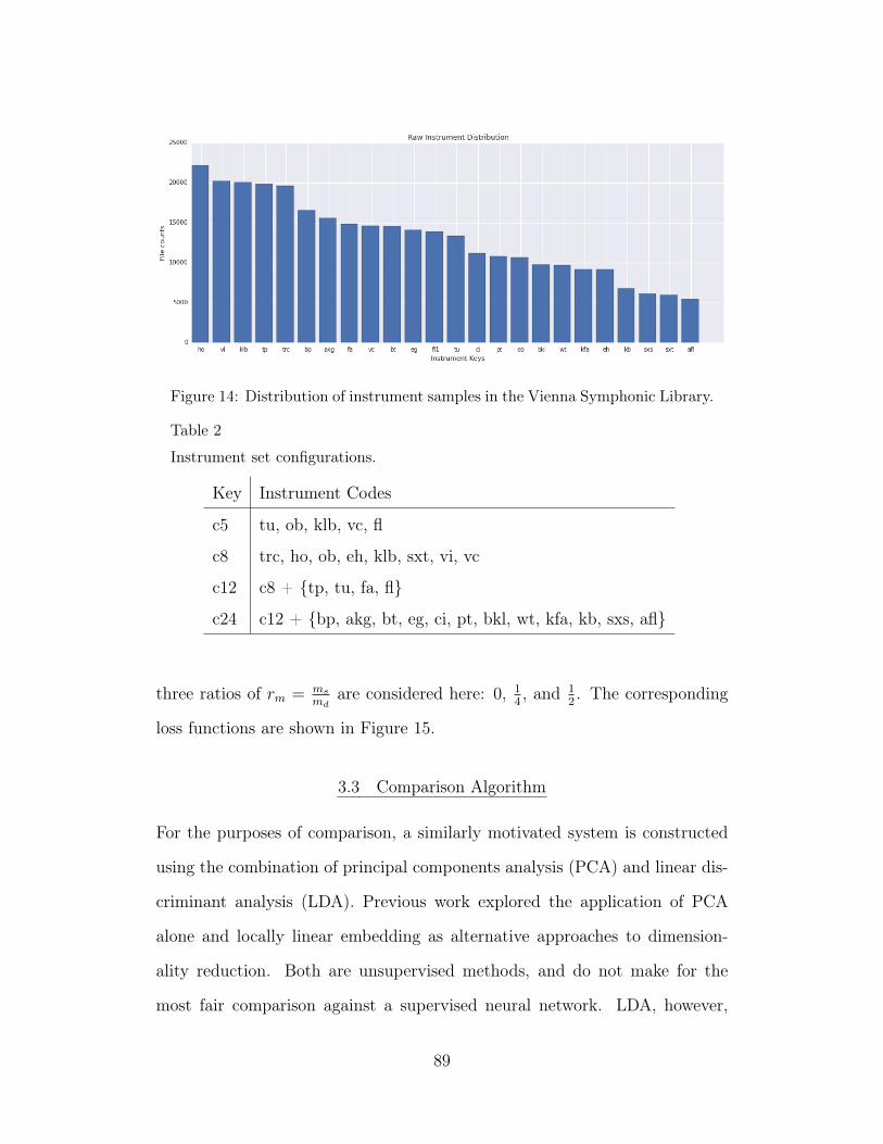
Figure 14: Distribution of instrument samples in the Vienna Symphonic Library.
Table 2
Instrument set configurations.
Key Instrument Codes
c5 tu, ob, klb, vc, fl
c8 trc, ho, ob, eh, klb, sxt, vi, vc
c12 c8 + {tp, tu, fa, fl}
c24 c12 + {bp, akg, bt, eg, ci, pt, bkl, wt, kfa, kb, sxs, afl}
three ratios of rm = ms
mdare considered here: 0, 1
4, and 1
2. The corresponding
loss functions are shown in Figure 15.
3.3 Comparison Algorithm
For the purposes of comparison, a similarly motivated system is constructed
using the combination of principal components analysis (PCA) and linear dis-
criminant analysis (LDA). Previous work explored the application of PCA
alone and locally linear embedding as alternative approaches to dimension-
ality reduction. Both are unsupervised methods, and do not make for the
most fair comparison against a supervised neural network. LDA, however,
89
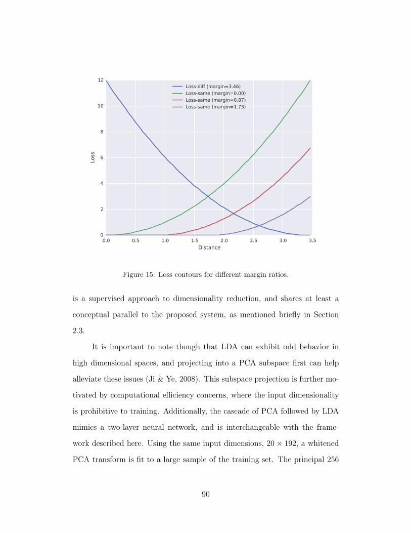
0.0 0.5 1.0 1.5 2.0 2.5 3.0 3.5
Distance
0
2
4
6
8
10
12
Loss
Loss-diff (margin=3.46)
Loss-same (margin=0.00)
Loss-same (margin=0.87)
Loss-same (margin=1.73)
Figure 15: Loss contours for different margin ratios.
is a supervised approach to dimensionality reduction, and shares at least a
conceptual parallel to the proposed system, as mentioned briefly in Section
2.3.
It is important to note though that LDA can exhibit odd behavior in
high dimensional spaces, and projecting into a PCA subspace first can help
alleviate these issues (Ji & Ye, 2008). This subspace projection is further mo-
tivated by computational efficiency concerns, where the input dimensionality
is prohibitive to training. Additionally, the cascade of PCA followed by LDA
mimics a two-layer neural network, and is interchangeable with the frame-
work described here. Using the same input dimensions, 20× 192, a whitened
PCA transform is fit to a large sample of the training set. The principal 256
90
components are preserved, based on an empirical exploration of the explained
variance as well as a midway point in the dimensionality reduction of the sys-
tem, i.e. the number of coefficients decreases near-equally between the PCA
and LDA stages. After applying the PCA transform to the training sample,
an LDA transform is fit to the same data and its corresponding instrument
classes, yielding a 3-dimensional embedding.
3.4 Experimental Results
As an initial quantitative inquiry, trained models are tested on a classification
task using the k-Nearest Neighbors classifier in scikit-learn∗. First, networks
are trained across the 4 instrument configurations, 3 margin ratios, and 5
folds, and all data are projected into the resulting embedding space. From
here, a collection of points are sampled from each partition —50k, 10k, 25k—
for training, validation, and test, respectively. The training set is used to fit
the classifier, while the validation set is used to identify an optimal setting for
the parameter k, corresponding to the number of neighbors considered in the
decision rule. Classification accuracy is then computed across all three sets,
and tallied across folds to produce averages and standard deviations across the
various conditions; these results are given in Tables 3-5.
A few conclusions are immediately obvious from these results. Most
striking is the performance discrepancy between the NLSE and the PCA-LDA
models. Previous work demonstrated a significant margin between the un-
supervised dimensionality reduction methods, and this result shows that the
difference is indeed a function of complexity, not just the supervised learning
∗http://scikit-learn.org/
91
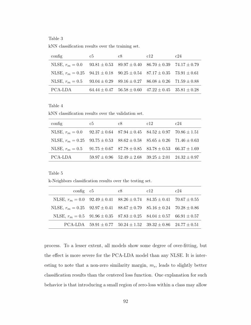
Table 3
kNN classification results over the training set.
config c5 c8 c12 c24
NLSE, rm = 0.0 93.81± 0.53 89.97± 0.40 86.70± 0.39 74.17± 0.79
NLSE, rm = 0.25 94.21± 0.18 90.25± 0.54 87.17± 0.35 73.91± 0.61
NLSE, rm = 0.5 93.04± 0.29 89.16± 0.27 86.08± 0.26 71.59± 0.88
PCA-LDA 64.44± 0.47 56.58± 0.60 47.22± 0.45 35.81± 0.28
Table 4
kNN classification results over the validation set.
config c5 c8 c12 c24
NLSE, rm = 0.0 92.37± 0.64 87.94± 0.45 84.52± 0.97 70.86± 1.51
NLSE, rm = 0.25 93.75± 0.53 88.62± 0.58 85.65± 0.26 71.46± 0.63
NLSE, rm = 0.5 91.75± 0.67 87.78± 0.85 83.78± 0.53 66.37± 1.69
PCA-LDA 59.97± 0.96 52.49± 2.68 39.25± 2.01 24.32± 0.97
Table 5
k-Neighbors classification results over the testing set.
config c5 c8 c12 c24
NLSE, rm = 0.0 92.49± 0.41 88.26± 0.74 84.35± 0.41 70.67± 0.55
NLSE, rm = 0.25 92.97± 0.41 88.67± 0.79 85.16± 0.24 70.28± 0.86
NLSE, rm = 0.5 91.96± 0.35 87.83± 0.25 84.04± 0.57 66.91± 0.57
PCA-LDA 59.91± 0.77 50.24± 1.52 39.32± 0.86 24.77± 0.51
process. To a lesser extent, all models show some degree of over-fitting, but
the effect is more severe for the PCA-LDA model than any NLSE. It is inter-
esting to note that a non-zero similarity margin, ms, leads to slightly better
classification results than the centered loss function. One explanation for such
behavior is that introducing a small region of zero-loss within a class may allow
92
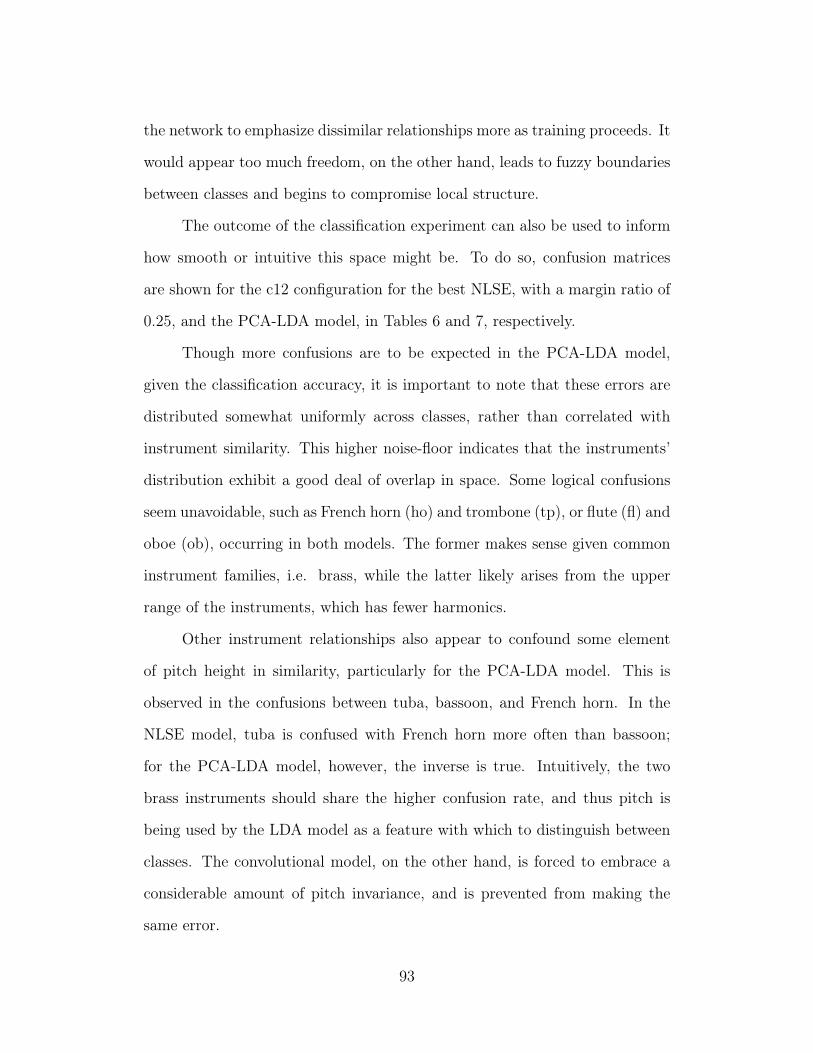
the network to emphasize dissimilar relationships more as training proceeds. It
would appear too much freedom, on the other hand, leads to fuzzy boundaries
between classes and begins to compromise local structure.
The outcome of the classification experiment can also be used to inform
how smooth or intuitive this space might be. To do so, confusion matrices
are shown for the c12 configuration for the best NLSE, with a margin ratio of
0.25, and the PCA-LDA model, in Tables 6 and 7, respectively.
Though more confusions are to be expected in the PCA-LDA model,
given the classification accuracy, it is important to note that these errors are
distributed somewhat uniformly across classes, rather than correlated with
instrument similarity. This higher noise-floor indicates that the instruments’
distribution exhibit a good deal of overlap in space. Some logical confusions
seem unavoidable, such as French horn (ho) and trombone (tp), or flute (fl) and
oboe (ob), occurring in both models. The former makes sense given common
instrument families, i.e. brass, while the latter likely arises from the upper
range of the instruments, which has fewer harmonics.
Other instrument relationships also appear to confound some element
of pitch height in similarity, particularly for the PCA-LDA model. This is
observed in the confusions between tuba, bassoon, and French horn. In the
NLSE model, tuba is confused with French horn more often than bassoon;
for the PCA-LDA model, however, the inverse is true. Intuitively, the two
brass instruments should share the higher confusion rate, and thus pitch is
being used by the LDA model as a feature with which to distinguish between
classes. The convolutional model, on the other hand, is forced to embrace a
considerable amount of pitch invariance, and is prevented from making the
same error.
93
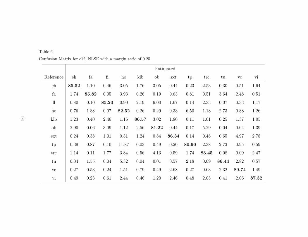
Table 6
Confusion Matrix for c12; NLSE with a margin ratio of 0.25.
Estimated
Reference eh fa fl ho klb ob sxt tp trc tu vc vi
eh 85.52 1.10 0.46 3.05 1.76 3.05 0.44 0.23 2.53 0.30 0.51 1.64
fa 1.74 85.82 0.05 3.93 0.26 0.19 0.63 0.81 0.51 3.64 2.48 0.51
fl 0.80 0.10 85.20 0.90 2.19 6.00 1.67 0.14 2.33 0.07 0.33 1.17
ho 0.76 1.88 0.07 82.52 0.26 0.29 0.33 6.50 1.18 2.73 0.88 1.26
klb 1.23 0.40 2.46 1.16 86.57 3.02 1.80 0.11 1.01 0.25 1.37 1.05
ob 2.90 0.06 3.09 1.12 2.56 81.22 0.44 0.17 5.29 0.04 0.04 1.39
sxt 0.24 0.38 1.01 0.51 1.24 0.84 86.34 0.14 0.48 0.65 4.97 2.78
tp 0.39 0.87 0.10 11.87 0.03 0.49 0.20 80.96 2.38 2.73 0.95 0.59
trc 1.14 0.11 1.77 3.84 0.56 4.13 0.59 1.74 83.45 0.08 0.09 2.47
tu 0.04 1.55 0.04 5.32 0.04 0.01 0.57 2.18 0.09 86.44 2.82 0.57
vc 0.27 0.53 0.24 1.51 0.79 0.49 2.68 0.27 0.63 2.32 89.74 1.49
vi 0.49 0.23 0.61 2.44 0.46 1.20 2.46 0.48 2.05 0.41 2.06 87.32
94
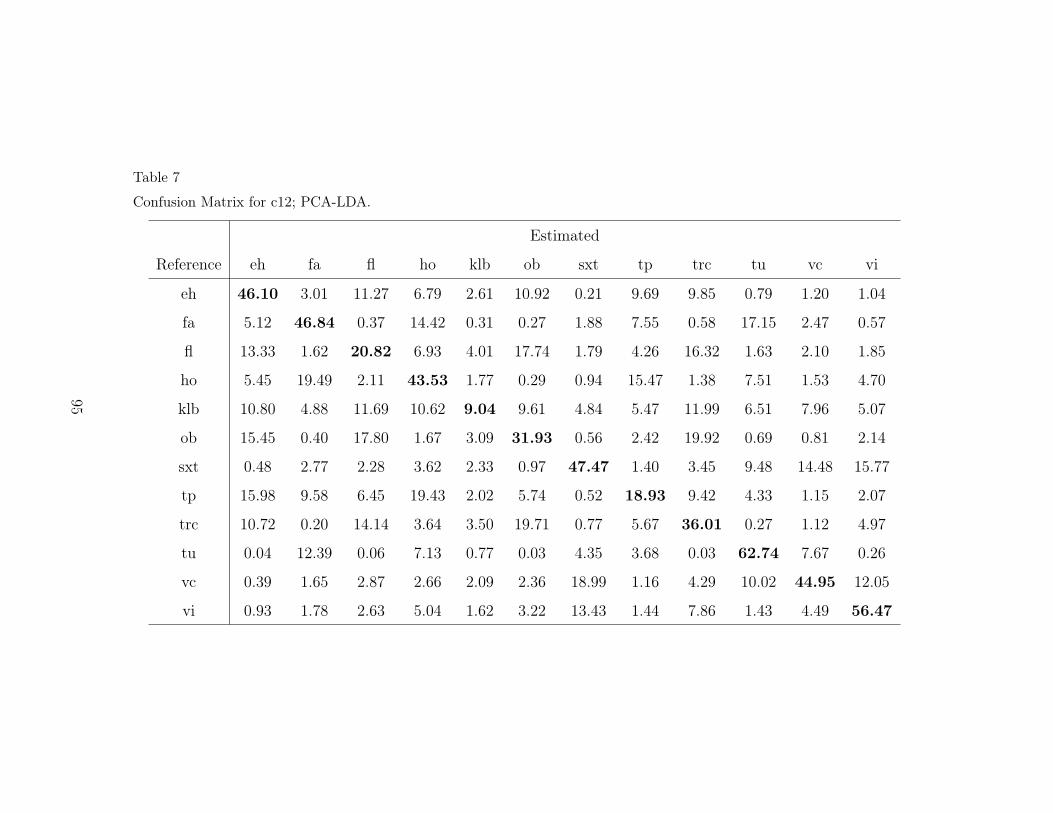
Table 7
Confusion Matrix for c12; PCA-LDA.
Estimated
Reference eh fa fl ho klb ob sxt tp trc tu vc vi
eh 46.10 3.01 11.27 6.79 2.61 10.92 0.21 9.69 9.85 0.79 1.20 1.04
fa 5.12 46.84 0.37 14.42 0.31 0.27 1.88 7.55 0.58 17.15 2.47 0.57
fl 13.33 1.62 20.82 6.93 4.01 17.74 1.79 4.26 16.32 1.63 2.10 1.85
ho 5.45 19.49 2.11 43.53 1.77 0.29 0.94 15.47 1.38 7.51 1.53 4.70
klb 10.80 4.88 11.69 10.62 9.04 9.61 4.84 5.47 11.99 6.51 7.96 5.07
ob 15.45 0.40 17.80 1.67 3.09 31.93 0.56 2.42 19.92 0.69 0.81 2.14
sxt 0.48 2.77 2.28 3.62 2.33 0.97 47.47 1.40 3.45 9.48 14.48 15.77
tp 15.98 9.58 6.45 19.43 2.02 5.74 0.52 18.93 9.42 4.33 1.15 2.07
trc 10.72 0.20 14.14 3.64 3.50 19.71 0.77 5.67 36.01 0.27 1.12 4.97
tu 0.04 12.39 0.06 7.13 0.77 0.03 4.35 3.68 0.03 62.74 7.67 0.26
vc 0.39 1.65 2.87 2.66 2.09 2.36 18.99 1.16 4.29 10.02 44.95 12.05
vi 0.93 1.78 2.63 5.04 1.62 3.22 13.43 1.44 7.86 1.43 4.49 56.47
95
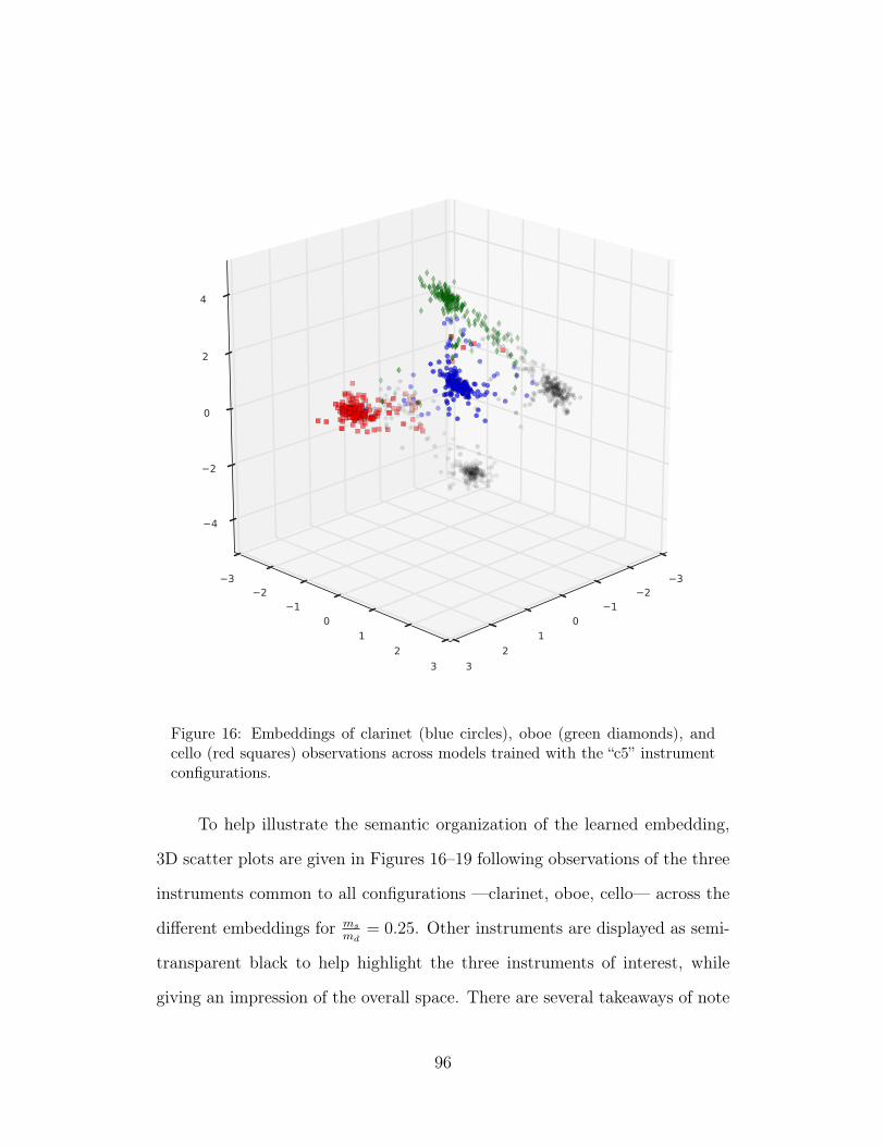
32
10
1
2
3
32
10
1
2
3
4
2
0
2
4
Figure 16: Embeddings of clarinet (blue circles), oboe (green diamonds), andcello (red squares) observations across models trained with the “c5” instrumentconfigurations.
To help illustrate the semantic organization of the learned embedding,
3D scatter plots are given in Figures 16–19 following observations of the three
instruments common to all configurations —clarinet, oboe, cello— across the
different embeddings for ms
md= 0.25. Other instruments are displayed as semi-
transparent black to help highlight the three instruments of interest, while
giving an impression of the overall space. There are several takeaways of note
96
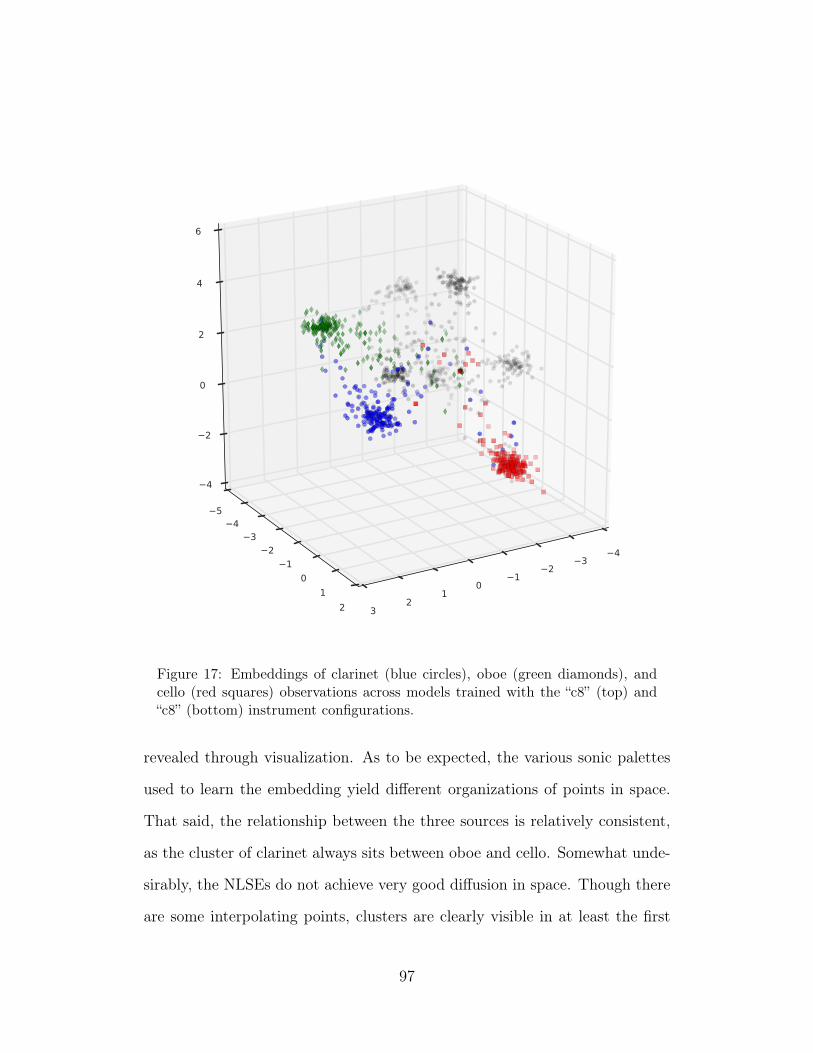
43
21
01
23
54
3
2
1
0
1
2
4
2
0
2
4
6
Figure 17: Embeddings of clarinet (blue circles), oboe (green diamonds), andcello (red squares) observations across models trained with the “c8” (top) and“c8” (bottom) instrument configurations.
revealed through visualization. As to be expected, the various sonic palettes
used to learn the embedding yield different organizations of points in space.
That said, the relationship between the three sources is relatively consistent,
as the cluster of clarinet always sits between oboe and cello. Somewhat unde-
sirably, the NLSEs do not achieve very good diffusion in space. Though there
are some interpolating points, clusters are clearly visible in at least the first
97
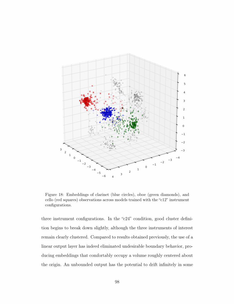
65
43
21
01
23
43
21
01
23
4
3
2
1
0
1
2
3
4
5
6
Figure 18: Embeddings of clarinet (blue circles), oboe (green diamonds), andcello (red squares) observations across models trained with the “c12” instrumentconfigurations.
three instrument configurations. In the “c24” condition, good cluster defini-
tion begins to break down slightly, although the three instruments of interest
remain clearly clustered. Compared to results obtained previously, the use of a
linear output layer has indeed eliminated undesirable boundary behavior, pro-
ducing embeddings that comfortably occupy a volume roughly centered about
the origin. An unbounded output has the potential to drift infinitely in some
98
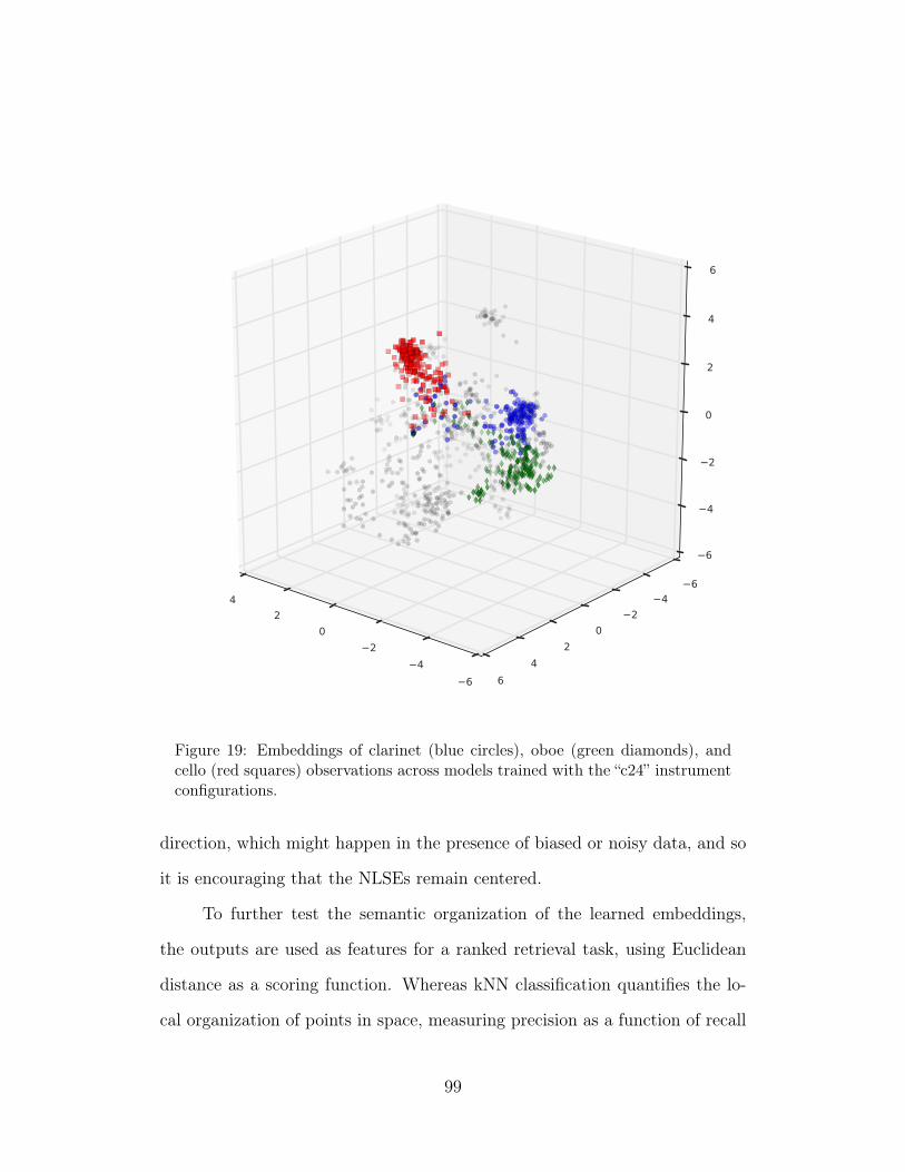
6
4
2
0
2
4
6
4
2
0
2
4
6
6
4
2
0
2
4
6
Figure 19: Embeddings of clarinet (blue circles), oboe (green diamonds), andcello (red squares) observations across models trained with the “c24” instrumentconfigurations.
direction, which might happen in the presence of biased or noisy data, and so
it is encouraging that the NLSEs remain centered.
To further test the semantic organization of the learned embeddings,
the outputs are used as features for a ranked retrieval task, using Euclidean
distance as a scoring function. Whereas kNN classification quantifies the lo-
cal organization of points in space, measuring precision as a function of recall
99
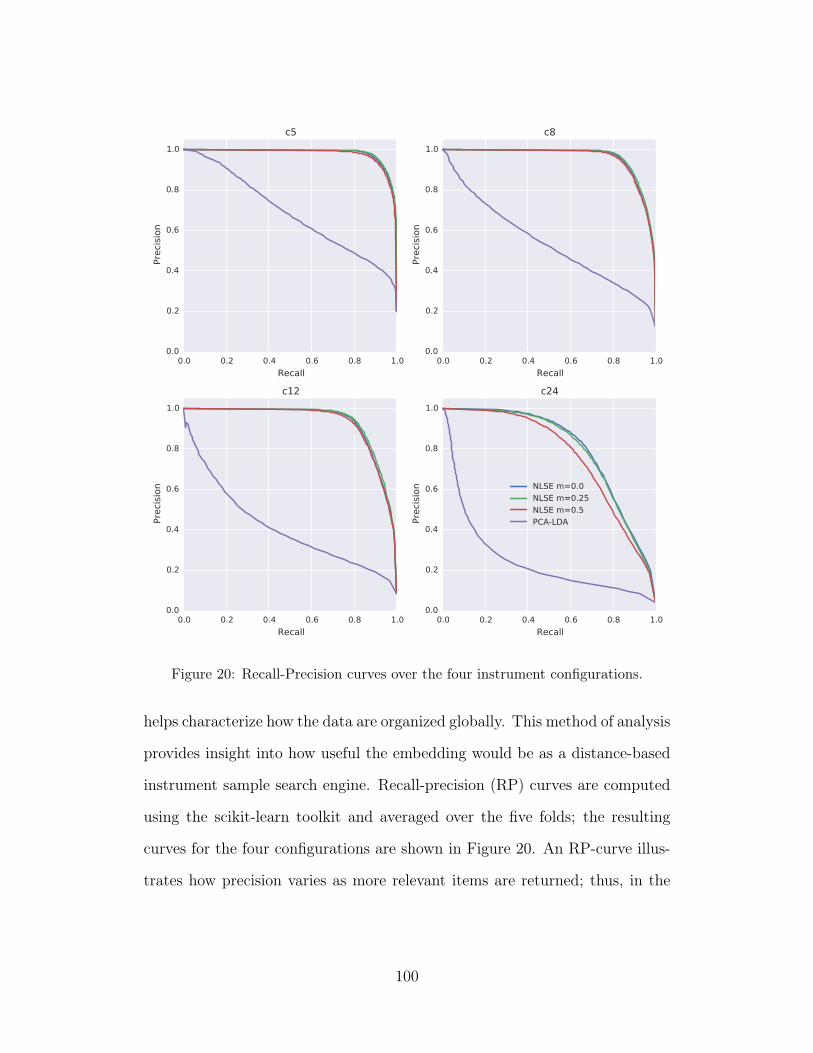
0.0 0.2 0.4 0.6 0.8 1.0
Recall
0.0
0.2
0.4
0.6
0.8
1.0Pre
cisi
on
c5
0.0 0.2 0.4 0.6 0.8 1.0
Recall
0.0
0.2
0.4
0.6
0.8
1.0
Pre
cisi
on
c8
0.0 0.2 0.4 0.6 0.8 1.0
Recall
0.0
0.2
0.4
0.6
0.8
1.0
Pre
cisi
on
c12
0.0 0.2 0.4 0.6 0.8 1.0
Recall
0.0
0.2
0.4
0.6
0.8
1.0Pre
cisi
on
c24
NLSE m=0.0
NLSE m=0.25
NLSE m=0.5
PCA-LDA
Figure 20: Recall-Precision curves over the four instrument configurations.
helps characterize how the data are organized globally. This method of analysis
provides insight into how useful the embedding would be as a distance-based
instrument sample search engine. Recall-precision (RP) curves are computed
using the scikit-learn toolkit and averaged over the five folds; the resulting
curves for the four configurations are shown in Figure 20. An RP-curve illus-
trates how precision varies as more relevant items are returned; thus, in the
100
ideal condition, an RP-curve approaches the upper-right corner of the plot,
versus the lower-left in the worst-case scenario.
Given the classification accuracy and confusion matrices above, the per-
formance gap between the NLSE and PCA-LDA models is unsurprising. Still,
it is interesting to consider what the shape of these recall-precision curves indi-
cates. The two characteristics to observe are the concavity of the contour and
the “knee” at which it breaks downward. In all instrument configurations, with
the slight exception of “c5”, the NLSE models and the PCA-LDA model exhibit
opposite second-derivatives. This behavior can be understood as the acceler-
ation with which precision changes as a function of recall. For the NLSEs,
precision degrades slowly until reaching a crossover point, referred to here as
the knee, where precision drops off rapidly. The PCA-LDA model does the op-
posite, where precision drops quickly close to a query point, and slows as recall
increases. Therefore, as encouraged by the visualizations, the NLSEs contain
better separated class clusters than the PCA-LDA embeddings. Furthermore,
the knee of a recall-precision curves belies an interesting region in the docu-
ment space, indicating that the edge of a cluster has been reached. This is
a useful observation for determining early-stopping criteria in the display of
ranked results, as well as identifying boundary regions in the embedding that
may present interesting opportunities for sonic exploration.
Looking to differences between NLSEs, there are two variables to con-
sider: instrument configuration and margin ratio. For the first three instru-
ment configurations, precision is roughly 100% out past a recall of 0.6; this
can be understood as the top 60% of results for a given query will correctly
match that instrument. In the final condition though, “c24”, this break occurs
just past a recall of 0.2, at which point other instrument samples would start
101
to appear in the list of results. This is still quite good from the perspective
of precision at the top of the ranked list, but it illustrates the point at which
the embedding space is beginning to get crowded. A higher dimensional em-
bedding might alleviate this at the expense of visualization, but would still
be suitable for a retrieval system. With respect to the margin ratio, the first
three instrument conditions are again roughly equivalent, whereas “c24” begins
to show more contrast between the embeddings. In all conditions ms
md= 0.5
yields the lowest performing NLSE, and is most pronounced in the final con-
dition. This is consistent with expectation, because the larger value of ms
de-emphasizes the tightness of instrument clusters, causing more overlap be-
tween the different classes.
4 Conclusions
In this chapter, an approach to building a computational model of timbre sim-
ilarity was presented, which achieved three goals. First, the system is able to
automatically learn relevant signal level features, circumventing the challenge
posed by the lack of a constructive definition of timbre. Second, the resulting
timbre space is semantically well-organized, as demonstrated by classification
and ranked retrieval measures, and intuitive, based on a Euclidean notion of
distance in a dimensionality that can be easily visualized. Lastly, the space
is quantitatively smooth, such that what confusions exist correspond to in-
strument families or other like sounds. This was made possible by leveraging
objective information about a collection of sound sources, eliminating the need
for costly subjective ratings. Together, this approach to learning a timbre
102
space shows promise for visualization and user-facing applications, such as the
search and navigation of large sound libraries.
That said, there is considerable future work to be considered. All evalu-
ation performed here is quantitative, and arguably disconnected from all sub-
jective experience. User studies would serve to further investigate the ideas of
perceptual smoothness and if or how is obtained by the learned space. Efforts
to analyze the learned features may further help elucidate the latent factors
that contribute to the percept of timbre. Additionally, though this approach
is able to make use of objective instrument taxonomies, any similarity space
obtained through pairwise comparisons is always limited by the range of in-
puts considered. Therefore, in order to obtain a more general timbre space,
a much wider set of sound sources would need to be considered. Conversely,
the intended use case of such a system may provide a constrained palette with
which to operate, e.g. instrument sounds for recording engineers and environ-
mental sounds for acoustic ecologists. Finally, there are at least two other ways
the sound source information could be used to train a system in a supervised
manner. One, it may be advantageous to obtain subjective pairwise ratings
not between all possible sounds, but rather groups or classes of sounds. These
pairwise ratings could be used to train a system with soft, continuous-valued
similarity ratings, rather than the binary comparison scores used here. Two,
rather than defining an entire class to be similar, a hybrid approach to simi-
larity based on distance-based neighborhoods in the input space constrained
to a single class may also lead to interesting embeddings. It is unlikely such an
embedding would exhibit spherical clusters as was produced here, but points
are likely to be more uniformly distributed, or diffuse, in space.
103
CHAPTER V
AUTOMATIC CHORD ESTIMATION
The focus of this study now turns to automatic chord estimation (ACE),
one of the oldest subtopics in the field of content-based MIR. Complementing
the previous chapter, ACE presents a more challenging, well-worn problem
with a long research lineage and myriad applications. In addition to the stan-
dard objective of advancing the state of the art in a given application domain,
this chapter also aims to use deep learning to explore challenges inherent to
complex music intelligence tasks. Adopting a similar approach as before, deep
convolutional neural networks are used to estimate the likelihoods of different
chord classes from time-frequency representations of audio. A thorough inves-
tigation serves to not only offer insight into the application of deep learning
methods to future problems in content-based MIR, but also culminate in a
better understanding of the chord estimation task itself.
1 Context
In this section, the prerequisite knowledge relevant to a thorough treatment
of automatic chord estimation systems is addressed. First, a basic review
of Western tonal theory introduces core music concepts, and thus provides a
language with which to discuss the problem. This is followed by a brief outline
of the syntax used here to compactly notate chords. The problem domain is
then jointly motivated by potential use-cases and the observed needs of modern
104
musicians. Finally, known limitations are detailed to identify assumptions and
subsequently contextualize any conclusions drawn from this work.
1.1 Musical Foundations
To understand the chord estimation task is to understand the concepts on
which it is built. Therefore, given the significant emphasis on signal processing
and machine learning in this work, it is therefore valuable to provide a basic
review of chords and harmony for the benefit of the technical reader unfamiliar
with music theory.
The most atomic unit in the acoustic realm of chords is a tone, defined
here as a pitched sound object. Pitch is defined as the perceptual phenomena
whereby a sound stimulus can be matched to the frequency of a pure sinusoid,
known as the fundamental frequency (Krumhansl, 1979). As a result, sounds
can be naturally ordered by fundamental frequency on a scale from low to
high. An octave is defined as the doubling of a quantity, and exhibits a special
relationship in human perception by which two tones, differing in fundamen-
tal frequency by an integer power of 2, are perceived as being similar; this
phenomena is referred to as octave equivalence.
A note is the musical counterpart of a tone, and the two are related by
way of a tuning system. While there are a multiplicity of tuning systems, this
work will exclusively consider 12-Tone Equal Temperament, or 12-TET, named
for the 12 discrete, equally spaced tones within an octave. The relationship
between notes and tones in 12-TET is defined by the following:
fpitch = ftuning ∗ 2 exp(nindex − 48
N) (19)
105
where N is the number of notes per octave, nindex is an integer note index,
ftuning is a reference tuning frequency, in Hertz, and fpitch is the fundamental
frequency, in Hertz, of the corresponding tone. Standard contemporary tuning
equates A4 = 440Hz, although it should be noted that this is more convention
than rule and is subject to change. In 12-TET, the unique pitch classes within
an octave are named, given by the ordered set, P:
P = {C,C]/D[,D,D]/E[, E, F, F ]/G[,G,G]/A[,A,A]/B[,B} (20)
Here, sharps, ], and flats, [, are symbols used to indicate the raising
or lowering of a note by one semitone, respectively. Due to this particular
tuning system, some pitch classes can be spelled with either a sharp or a flat,
e.g. A] = B[, a property known as enharmonic equivalence. An absolute
note name, consisting of a pitch class, p, and an octave, o, is given by the
following as a function of absolute note index, such that nindex = 0 → C0,
nindex = 12 → C1, etc.:
p = P[mod(nindex, 12)]
o = b nindex/12 c
Most real music combines different notes, and thus it is useful to define
an interval as the relative semitone distance between two notes. Intervals are
critical in the understanding of harmony because they are generally perceived
as similar regardless of absolute pitch height. For example, the interval from
106
C5 to G5 sounds the same as the interval from F3 to C4, both being seven
semitones.
From here, three interdependent harmonic concepts are built through
the simultaneous and sequential combination of intervals: scales, chords, and
keys. It is crucial to recognize that each is an emergent quality of intervalic
relationships, and efforts to define one purely in terms of another are somewhat
circular. That said, an ordered set of intervals in known as a scale, of which
the diatonic is the most widely used in common practice music. It consists of
seven intervals, given by the following:
{+2,+2,+1,+2,+2,+2,+1}
Rotating this sequence circularly results in different modes, of which two
are common in contemporary popular music: major, with a rotation of 0; and
minor ∗, with a rotation to the right of 3. Each scales’ degrees are expressed
by the following, shown here as a semitone distance from a starting note:
major = {0, 2, 4, 5, 7, 9, 11, 12}
minor = {0, 2, 3, 5, 7, 8, 10, 12}
∗More accurately, this is the natural minor scale, but the distinction is not terribly importanthere.
107
The pitch class on which the scale starts is referred to the tonic, and
lends its name to the scale. The sequences in (1.1) can be used to recover a
scale by circularly indexing the set of pitch classes given in (20). To illustrate,
a C Major and A minor scale are given by the following:
Cmajor = {C,D,E, F,G,A,B}
Aminor = {A,B,C,D,E, F,G}
It should be noted that these two scales, despite different modes and tonics, are
composed of identical notes. These scales are known as each other’s relative
major and minor, respectively, and share a strong perceptual affinity.
Proceeding from scales, a chord is classically conceived as a simultane-
ous grouping of notes. One of the most important chord types in Western
tonal theory is the triad, on which many other theoretical constructs are built.
Comprised of three notes, a triad is built by taking the third and fifth scale
degrees from a chosen starting point, referred to as the root. For example, this
expansion is given for the major scale in Table 8.
For a given chord, the root is defined as the home note on which the
intervals are stacked, and the quality determined by the relationship of the
intervals to the root. An interval of 4 semitones is known as a major third and
3 semitones a minor third, sharing a commonality with the third scale degree
of the major and minor scales, respectively. Therefore, the qualities of the first
six chords in the table are named for their relationship with the corresponding
108
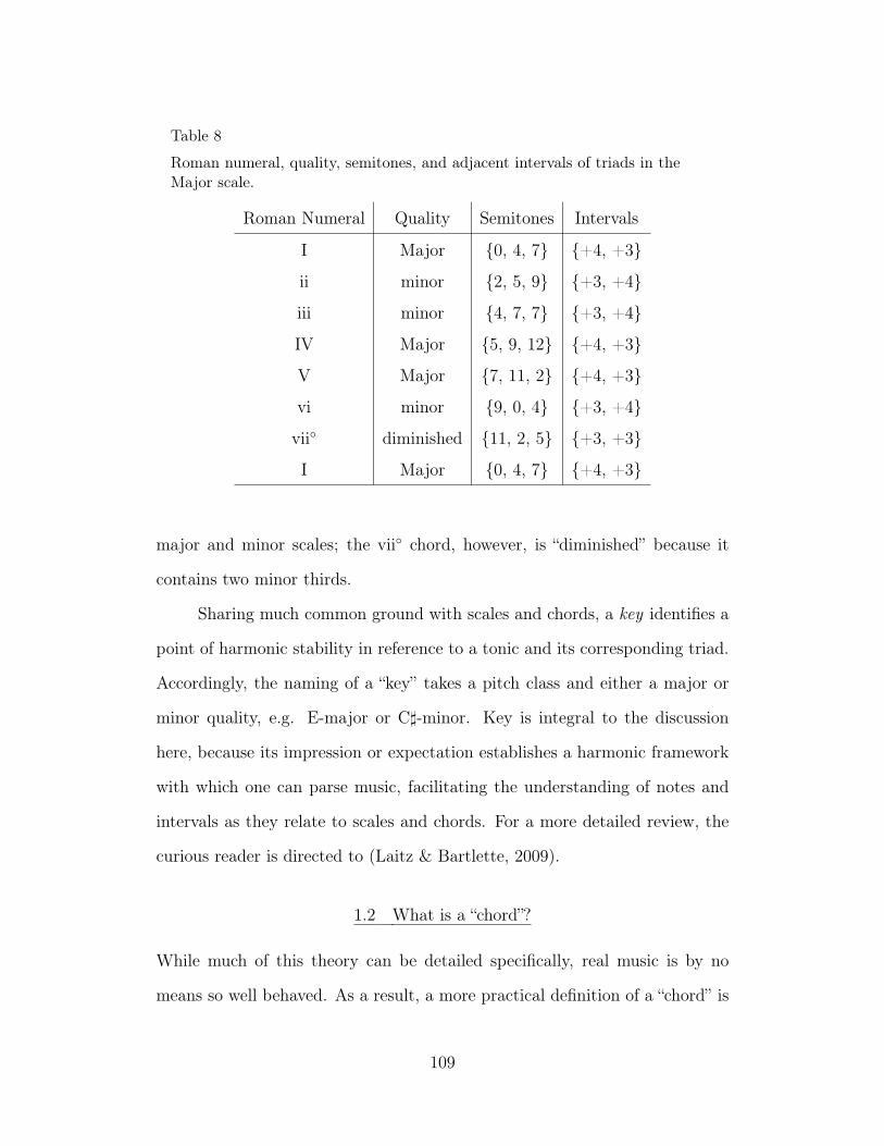
Table 8
Roman numeral, quality, semitones, and adjacent intervals of triads in theMajor scale.
Roman Numeral Quality Semitones Intervals
I Major {0, 4, 7} {+4, +3}
ii minor {2, 5, 9} {+3, +4}
iii minor {4, 7, 7} {+3, +4}
IV Major {5, 9, 12} {+4, +3}
V Major {7, 11, 2} {+4, +3}
vi minor {9, 0, 4} {+3, +4}
vii◦ diminished {11, 2, 5} {+3, +3}
I Major {0, 4, 7} {+4, +3}
major and minor scales; the vii◦ chord, however, is “diminished” because it
contains two minor thirds.
Sharing much common ground with scales and chords, a key identifies a
point of harmonic stability in reference to a tonic and its corresponding triad.
Accordingly, the naming of a “key” takes a pitch class and either a major or
minor quality, e.g. E-major or C]-minor. Key is integral to the discussion
here, because its impression or expectation establishes a harmonic framework
with which one can parse music, facilitating the understanding of notes and
intervals as they relate to scales and chords. For a more detailed review, the
curious reader is directed to (Laitz & Bartlette, 2009).
1.2 What is a “chord”?
While much of this theory can be detailed specifically, real music is by no
means so well behaved. As a result, a more practical definition of a “chord” is
109
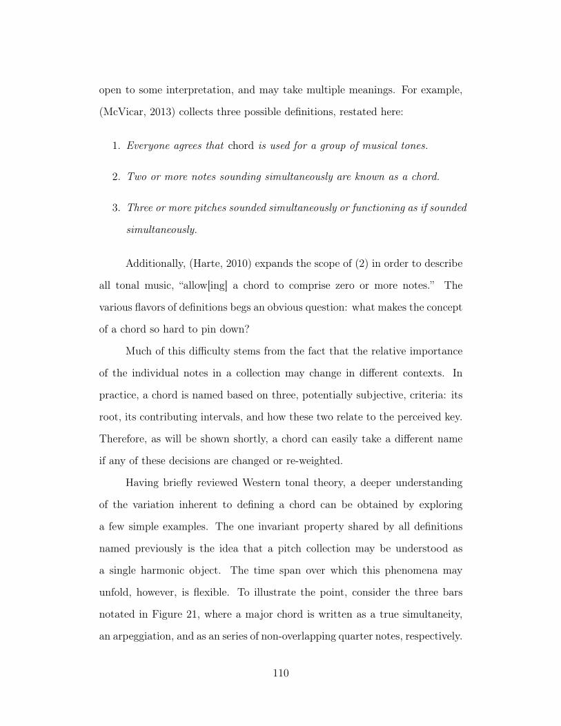
open to some interpretation, and may take multiple meanings. For example,
(McVicar, 2013) collects three possible definitions, restated here:
1. Everyone agrees that chord is used for a group of musical tones.
2. Two or more notes sounding simultaneously are known as a chord.
3. Three or more pitches sounded simultaneously or functioning as if sounded
simultaneously.
Additionally, (Harte, 2010) expands the scope of (2) in order to describe
all tonal music, “allow[ing] a chord to comprise zero or more notes.” The
various flavors of definitions begs an obvious question: what makes the concept
of a chord so hard to pin down?
Much of this difficulty stems from the fact that the relative importance
of the individual notes in a collection may change in different contexts. In
practice, a chord is named based on three, potentially subjective, criteria: its
root, its contributing intervals, and how these two relate to the perceived key.
Therefore, as will be shown shortly, a chord can easily take a different name
if any of these decisions are changed or re-weighted.
Having briefly reviewed Western tonal theory, a deeper understanding
of the variation inherent to defining a chord can be obtained by exploring
a few simple examples. The one invariant property shared by all definitions
named previously is the idea that a pitch collection may be understood as
a single harmonic object. The time span over which this phenomena may
unfold, however, is flexible. To illustrate the point, consider the three bars
notated in Figure 21, where a major chord is written as a true simultaneity,
an arpeggiation, and as an series of non-overlapping quarter notes, respectively.
110
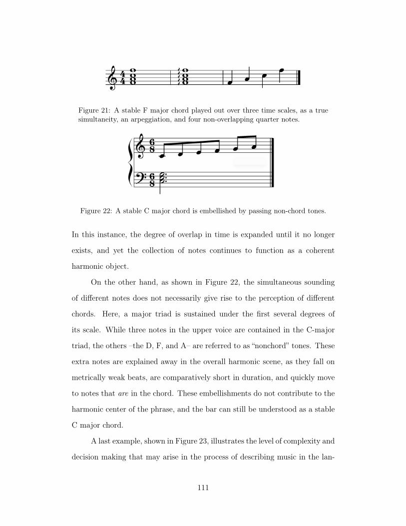
Figure 21: A stable F major chord played out over three time scales, as a truesimultaneity, an arpeggiation, and four non-overlapping quarter notes.
Figure 22: A stable C major chord is embellished by passing non-chord tones.
In this instance, the degree of overlap in time is expanded until it no longer
exists, and yet the collection of notes continues to function as a coherent
harmonic object.
On the other hand, as shown in Figure 22, the simultaneous sounding
of different notes does not necessarily give rise to the perception of different
chords. Here, a major triad is sustained under the first several degrees of
its scale. While three notes in the upper voice are contained in the C-major
triad, the others –the D, F, and A– are referred to as “nonchord” tones. These
extra notes are explained away in the overall harmonic scene, as they fall on
metrically weak beats, are comparatively short in duration, and quickly move
to notes that are in the chord. These embellishments do not contribute to the
harmonic center of the phrase, and the bar can still be understood as a stable
C major chord.
A last example, shown in Figure 23, illustrates the level of complexity and
decision making that may arise in the process of describing music in the lan-
111
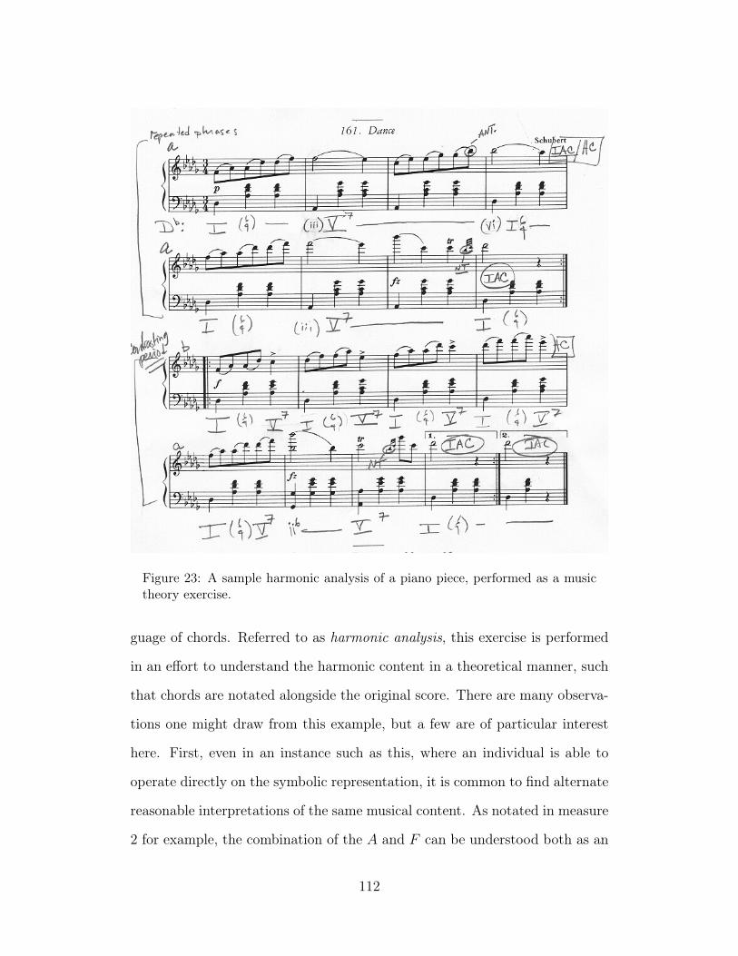
Figure 23: A sample harmonic analysis of a piano piece, performed as a musictheory exercise.
guage of chords. Referred to as harmonic analysis, this exercise is performed
in an effort to understand the harmonic content in a theoretical manner, such
that chords are notated alongside the original score. There are many observa-
tions one might draw from this example, but a few are of particular interest
here. First, even in an instance such as this, where an individual is able to
operate directly on the symbolic representation, it is common to find alternate
reasonable interpretations of the same musical content. As notated in measure
2 for example, the combination of the A and F can be understood both as an
112
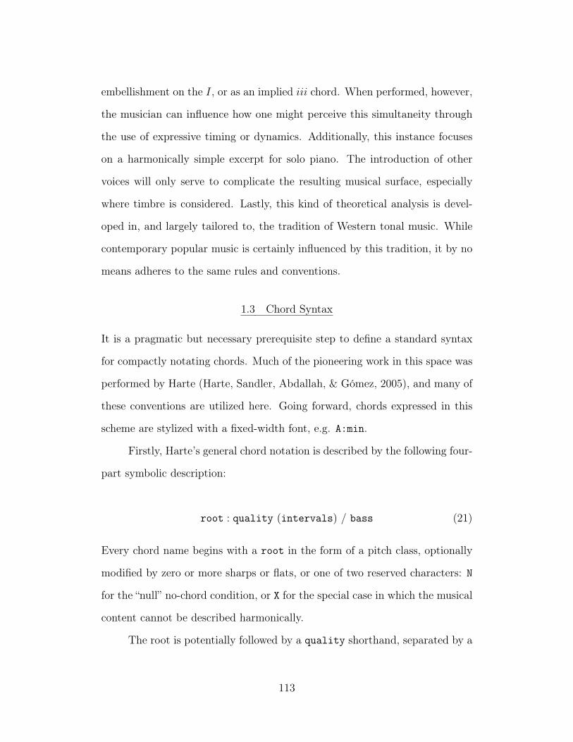
embellishment on the I, or as an implied iii chord. When performed, however,
the musician can influence how one might perceive this simultaneity through
the use of expressive timing or dynamics. Additionally, this instance focuses
on a harmonically simple excerpt for solo piano. The introduction of other
voices will only serve to complicate the resulting musical surface, especially
where timbre is considered. Lastly, this kind of theoretical analysis is devel-
oped in, and largely tailored to, the tradition of Western tonal music. While
contemporary popular music is certainly influenced by this tradition, it by no
means adheres to the same rules and conventions.
1.3 Chord Syntax
It is a pragmatic but necessary prerequisite step to define a standard syntax
for compactly notating chords. Much of the pioneering work in this space was
performed by Harte (Harte, Sandler, Abdallah, & Gómez, 2005), and many of
these conventions are utilized here. Going forward, chords expressed in this
scheme are stylized with a fixed-width font, e.g. A:min.
Firstly, Harte’s general chord notation is described by the following four-
part symbolic description:
root : quality (intervals) / bass (21)
Every chord name begins with a root in the form of a pitch class, optionally
modified by zero or more sharps or flats, or one of two reserved characters: N
for the “null” no-chord condition, or X for the special case in which the musical
content cannot be described harmonically.
The root is potentially followed by a quality shorthand, separated by a
113
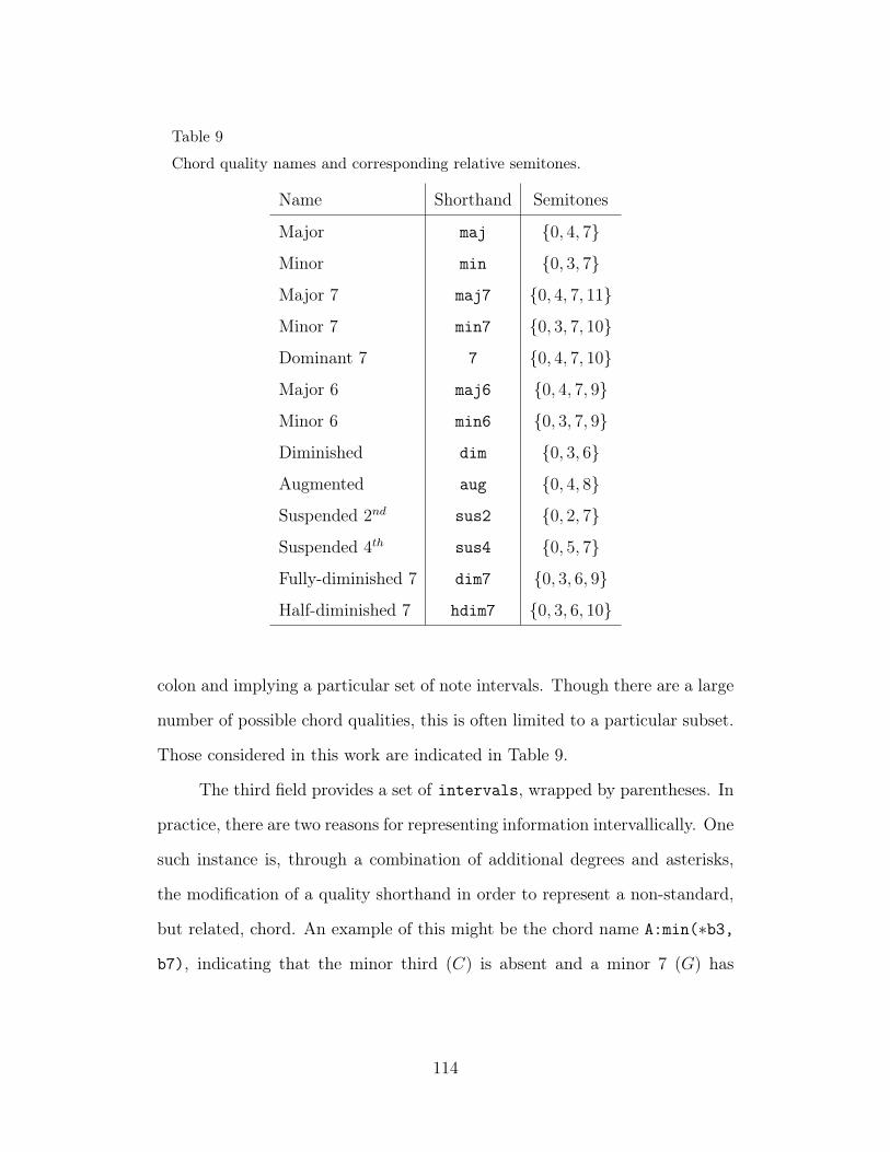
Table 9
Chord quality names and corresponding relative semitones.
Name Shorthand Semitones
Major maj {0, 4, 7}
Minor min {0, 3, 7}
Major 7 maj7 {0, 4, 7, 11}
Minor 7 min7 {0, 3, 7, 10}
Dominant 7 7 {0, 4, 7, 10}
Major 6 maj6 {0, 4, 7, 9}
Minor 6 min6 {0, 3, 7, 9}
Diminished dim {0, 3, 6}
Augmented aug {0, 4, 8}
Suspended 2nd sus2 {0, 2, 7}
Suspended 4th sus4 {0, 5, 7}
Fully-diminished 7 dim7 {0, 3, 6, 9}
Half-diminished 7 hdim7 {0, 3, 6, 10}
colon and implying a particular set of note intervals. Though there are a large
number of possible chord qualities, this is often limited to a particular subset.
Those considered in this work are indicated in Table 9.
The third field provides a set of intervals, wrapped by parentheses. In
practice, there are two reasons for representing information intervallically. One
such instance is, through a combination of additional degrees and asterisks,
the modification of a quality shorthand in order to represent a non-standard,
but related, chord. An example of this might be the chord name A:min(∗b3,
b7), indicating that the minor third (C) is absent and a minor 7 (G) has
114
been added. The other instance occurs when the intervals are certain but the
quality is ambiguous, such as C:(1, 5).
The final field of this chord syntax is the bass interval, which indicates
the scale degree of the lowest contributing pitch. Typically this is also the root
of the chord, and is implied as such in the absence of an explicit bass interval.
However, it is necessary to state that the scale degrees of the chord —given by
the quality shorthand and the interval set— can be further augmented by the
inclusion of a bass interval. For example, the chords C:maj/b7 and C:7 would
be understood as containing the same pitch classes, but are spelled differently.
1.4 Motivation
Even from the earliest efforts in content-based MIR, automatic music tran-
scription has stood as one of the Holy Grails of the field. Time would prove
this to be an exceptionally difficult problem, and fracture this common cause
into a variety of smaller, and hopefully more manageable, subtopics. Auto-
matic chord estimation materialized as one such task, now receiving healthy
attention for more than a decade, and is established as a benchmark challenge
at the annual MIReX event∗.
Given the prerequisite skill necessary to produce chord transcriptions
manually from recorded audio, there is considerable motivation to develop
automated systems capable of reliably performing this task. As evidenced
by large online communities surrounding websites like e-chords† or Ultimate
Guitar‡, countless individuals invest considerable time and effort in the cura-
∗http://www.music-ir.org/mirex/wiki/MIREX_HOME†http://www.e-chords.com‡http://www.ultimate-guitar.com
115
tion and consumption of popular music transcriptions. Often this is driven
by desire to learn and perform music for which symbolic notation does not
exist. Conversely, automatic chord estimation systems would be particularly
useful in the areas of composition, recording, and production. Furthermore,
the curation of this content would enable large-scale musicological analysis of
contemporary music.
In addition to the concerns of individual users, computational systems
capable of reliable chord estimation are directly useful inside the domain of
content-based MIR. Chords can serve as a robust mid-level representation with
which to build systems and extract higher level musical knowledge, and have
been used for cover song retrieval (Bello, 2007) and genre recognition (Anglade,
Ramirez, & Dixon, 2009). Such systems would also facilitate data collection
for other tasks, aiding in visualization and other facets of music transcription.
From a more philosophical perspective, the identification of chords is
also intriguing as an intelligent musical behavior, being a high level cognitive
process that is often open to multiple interpretations between knowledgeable
experts. Experiential bias of the annotator may manifest in the subjective
decisions made by an observer, where a pianist may arrive at a different har-
monic analysis than that of a guitarist due to how a collection of notes might
be produced. Finally, the knowledge and skill of the one recognizing chords
in music will affect the resulting interpretations. Beginners will likely prefer
simple or more common descriptions, whereas experts will be more aware of
complex nuances and have better command over a larger harmonic vocabulary.
116
1.5 Limitations
It should be acknowledged that this inquiry is subject to the limitations of
tonal theory and chords as a language with which to describe a piece of music.
Primarily, this work is interested in the tradition of tonal Western music, with
a particular focus on popular contemporary music from the last century, in
12-TET. Within this large body of music content, the use of harmony and
chords has steadily evolved over time. Classically, music theorists have long
sought to characterize musical works via analysis and reduction as a means
to understanding, typically operating from a symbolic representations, i.e. a
score. As a result, the language of “chords” developed as an expressive, yet
compact, language with which one might describe a piece of music harmoni-
cally. However, Western “pop music”, infused with elements of folk, blues, jazz,
rock and countless other influences, is not to required to adhere to or consider
the rules of traditional tonal theory (Tagg, 1982). Thus efforts to understand
the former in the language of the latter is ultimately limited by the validity in
doing so.
Even in the constrained space of Western tonal music set forth here, not
all musical works will be well-described by the language of harmonic analysis,
and thus chords may be a clumsy language with which to describe such music.
An alternative approach to analysis, such as voice leading, might make more
sense in this instance; in others, such as “math rock”, a lack of clearly structured
harmonic content may arguably render the goal of harmonic analysis irrelevant
(Cateforis, 2002). As genre is itself an amorphous and ill-defined concept, the
degree to which a piece of music might be understood harmonically will vary,
both absolutely and internally.
117
2 Previous Research in Automatic Chord Estimation
Building upon the conceptual foundations addressed previously, automatic
chord estimation research can be described in three parts. First, an effort is
made to formally define the goals of computational systems. The research
lineage is then surveyed, identifying commonalities between this work and
highlighting the state of the art. Approaches to evaluation methodology are
discussed last, including a review of data used to benchmark the research
presented here.
2.1 Problem Formulation
Following the motivations outlined in 1.4, the goal of an automatic chord
estimation (ACE) system is –or, at least, has been– to produce “good” time-
aligned sequence of chords from a given music signal. As discussed in 1.3, it is
a particular nuance of chord notation that the space of valid spellings is effec-
tively infinite. To constrain the complexity of the task at hand, ACE systems
are traditionally designed to estimate chords from a finite vocabulary, defined
a priori. This simplification reduces the chord estimation to a classification
problem, where all observations are assigned to one of K chord classes.
Historically, the choice of chord vocabulary has been anything but stan-
dard, influenced primarily by the data available to a researcher. Supervised
machine learning approaches, for example, can be sensitive to the amount of
labeled data available for training, in which case it might be advantageous
to only consider sufficiently represented chord classes. Furthermore, not all
researchers have access to the same data, introducing another degree of vari-
118
ability. As a result, it can be challenging, if not impossible, to compare the
performance of systems designed for different chord vocabularies.
To address this challenge, one common strategy employed by the research
community is that of Major-Minor chord resolution. Based on the common
24 Major and minor keys, this formulation proceeds by mapping all chords in
a collection to either a Major or Minor chord with the same root (McVicar,
2013). While this results in some musically reasonable chord mappings, e.g.
maj7 → maj, others are more difficult to justify, e.g. dim7 → min or aug →
maj.
Having framed chord estimation as a classification problem, there are two
critical assumptions to note going forward. First, the classification paradigm
operates on the notion that the relationship between an observation and its cor-
responding class is stable. Chord estimation research has classically leveraged
expert musicians in the spirit of achieving objectivity, but this is ultimately an
approximation to some unknown degree. Second, flat classification problems
—those in which different classes are conceptually independent— are built on
the assumption of mutually exclusive relationships. In other words, assignment
to one class precludes the valid assignment to any other classes considered. For
example, “cat” and “dog” are mutually exclusive classes of “animal”, but “cat”
and “mammal” are not. Returning to chords, C:dim7 and C:maj are clearly
mutually exclusive classes, but it is difficult to say the same of C:maj7 and
C:maj, as the former contains the latter.
2.2 Computational Approaches
Considering the space of ACE research, it is observed by (Cho, 2014) all ap-
proaches to the task adopt the same basic architecture, diagrammed in Fig-
119
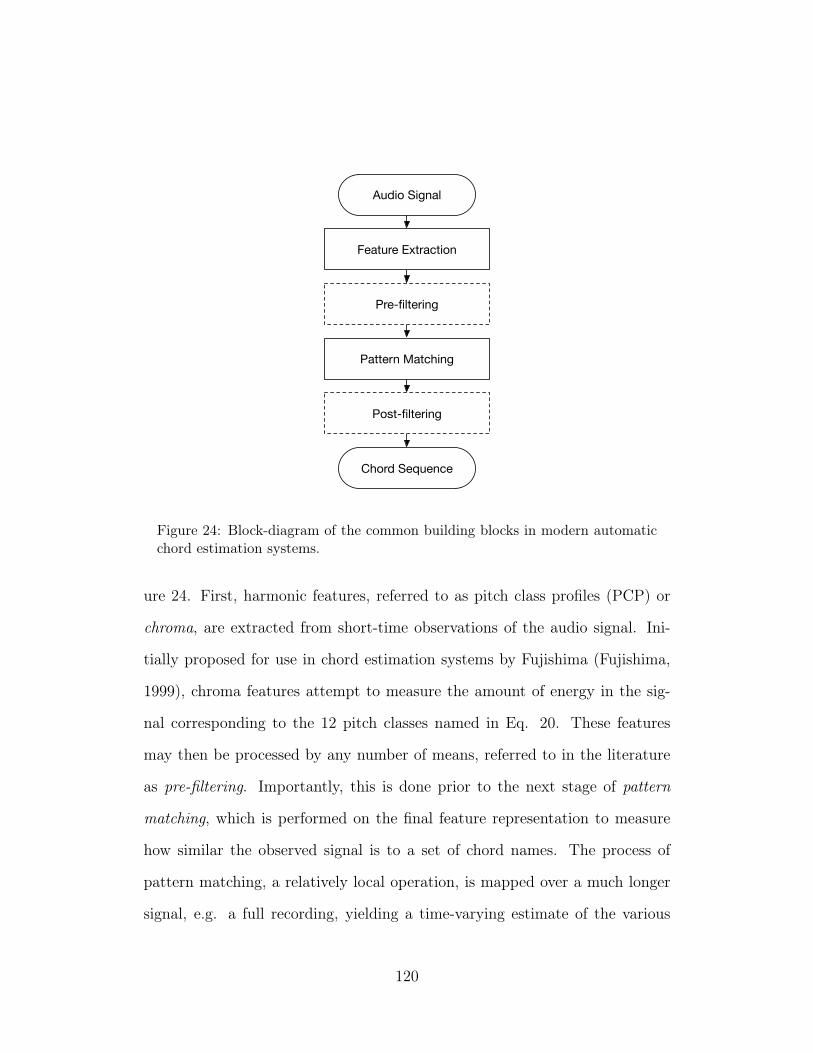
Feature Extraction
Audio Signal
Pattern Matching
Pre-filtering
Chord Sequence
Post-filtering
Figure 24: Block-diagram of the common building blocks in modern automaticchord estimation systems.
ure 24. First, harmonic features, referred to as pitch class profiles (PCP) or
chroma, are extracted from short-time observations of the audio signal. Ini-
tially proposed for use in chord estimation systems by Fujishima (Fujishima,
1999), chroma features attempt to measure the amount of energy in the sig-
nal corresponding to the 12 pitch classes named in Eq. 20. These features
may then be processed by any number of means, referred to in the literature
as pre-filtering. Importantly, this is done prior to the next stage of pattern
matching, which is performed on the final feature representation to measure
how similar the observed signal is to a set of chord names. The process of
pattern matching, a relatively local operation, is mapped over a much longer
signal, e.g. a full recording, yielding a time-varying estimate of the various
120
chord types the model can represent. Finally, post-filtering is applied to the
output of the pattern matching stage, resulting in a sequence of chord names
over time.
Though the implementation details have continued to evolve over the
last decade, the brunt of chord estimation research has concentrated not on
the fundamental system per se, but rather the tuning of its components. In
particular, much time and energy has been invested in developing not just bet-
ter features, but specifically better chroma features (Müller & Ewert, 2010).
Complementing chroma features, others have explored the use of multi-band
chroma to model bass frequencies separately (Mauch & Dixon, 2010b) or a
Tonnetz representation in an effort to better encode harmonic relationships
between chords (Lee & Slaney, 2007). Acknowledging the challenges inherent
to designing good features, Pachet et al pioneered work in automatic feature
optimization (Cabral & Pachet, 2006), and more recently deep learning meth-
ods have been employed to learn robust Tonnetz features (Humphrey, Cho, &
Bello, 2012). Early methods focused on local smoothing, such as low-pass or
median filtering as a form of pre-filtering (Cho et al., 2010), but more recently
some methods have attempted to leverage the repeated nature of music to
yield more stable estimates of the harmonic composition at a given point in
time (Cho & Bello, 2011). Various classification strategies have been inves-
tigated such as binary templates (Oudre, Grenier, & Févotte, 2009), Dirich-
let distribution models (Burgoyne & Saul, 2005), or Support Vector Machines
(SVMs) (Weller, Ellis, & Jebara, 2009), but Gaussian Mixture Models (GMM)
are by and large the most common feature modeling approach (Cho, 2014).
The choice of post-filtering methods has been shown to significantly impact
system performance, and much research has focused on properly tuning Hid-
121
den Markov Models (HMMs) (Cho et al., 2010), first introduced by (Sheh
& Ellis, 2003). Recently, in an effort to continue to advance the state of
the art, researchers have begun exploring more complex post-filtering meth-
ods such as Dynamic Bayesian Networks (DBNs) (Mauch & Dixon, 2010a),
Conditional Random Fields (Sumi et al., 2012), and Variable-Length Markov
Models (Chordia et al., 2011).
It is worth noting that in this lineage, the systems that do make use of
data-driven learning typically only do so in disjoint stages. More often than
not, machine learning is only performed at the pattern matching stage, where
increasingly powerful models are fit to hand-crafted features. A few works do
attempt to learn features, such as (Mauch & Dixon, 2010a; Humphrey, Cho,
& Bello, 2012), but the different stages are optimized independently. Though
it is standard practice to train a GMM/HMM jointly, some have observed
that learning the parameters of the HMM, i.e. the transition probabilities,
yields no significant benefit over a uniform probabilities with a strong self-
transition affinity (Cho, 2014). One notable work that attempts to jointly
optimize multiple stages is that of (Cho, Kim, & Bello, 2012), which optimizes
the GMM to a minimum frame classification error, rather than a conventional
maximum likelihood formulation.
2.3 Evaluation Methodology
In order to objectively measure the quality of a proposed ACE system, it is
necessary to address two related components: the collection of ground-truth
data, and the manner in which estimations are compared to this reference
data.
The first major effort to curate ground truth chord transcriptions was
122
led by Harte in the mid-2000s, referred to as the Isophonics dataset∗, where
a small team of researchers transcribed the entire discography of The Beatles.
Containing chord annotations for 180 tracks, this was a landmark dataset
in the field of MIR and shaped years of ACE research. Importantly, this
transcription effort leveraged professional transcriptions of the music under
consideration, and was verified for accuracy multiple times. However, despite
this rigor, the data is drawn from a single artist and very well known to
the research community; some have argued that ACE research has begun to
manually overfit this collection.
To combat these issues, two datasets were released following the 2011
Conference of the International Society of Music Information Retrieval (IS-
MIR), one of over 700 tracks led by J. Ashley Burgoyne (Burgoyne, Wild, &
Fujinaga, 2011) and another of 295 tracks led by Tae Min Cho, from the Music
and Audio Research Lab at NYU†; here, the former is referred to as “Billboard”
and the latter as “MARL-Chords”, corresponding to their related projects. In
parallel, an additional, comparatively small, dataset was released, containing
20 tracks by the band Queen, provided by Matthias Mauch as an extension to
the Isophonics set. In all four cases, the chord transcriptions are provided as
“ground truth”, on the premise that the data corresponds to the expert per-
spective. To help prevent errors and resolve judgment calls, these additional
annotation efforts employed a review process, where the transcriptions of one
or more annotators were verified by a different individual.
Leveraging this ground truth data, it is possible to quantitatively assess
∗http://isophonics.net/content/reference-annotations†https://github.com/tmc323/Chord-Annotations
123
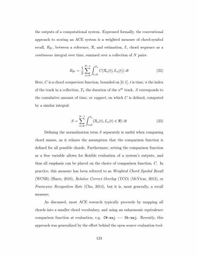
the outputs of a computational system. Expressed formally, the conventional
approach to scoring an ACE system is a weighted measure of chord-symbol
recall, RW , between a reference, R, and estimation, E, chord sequence as a
continuous integral over time, summed over a collection of N pairs:
RW =1
S
N−1∑n=0
∫ Tn
t=0
C(Rn(t),En(t)) dt (22)
Here, C is a chord comparison function, bounded on [0, 1], t is time, n the index
of the track in a collection, Tn the duration of the nth track. S corresponds to
the cumulative amount of time, or support, on which C is defined, computed
by a similar integral:
S =N−1∑n=0
∫ Tn
t=0
(Rn(t),En(t) ∈ <) dt (23)
Defining the normalization term S separately is useful when comparing
chord names, as it relaxes the assumption that the comparison function is
defined for all possible chords. Furthermore, setting the comparison function
as a free variable allows for flexible evaluation of a system’s outputs, and
thus all emphasis can be placed on the choice of comparison function, C. In
practice, this measure has been referred to as Weighted Chord Symbol Recall
(WCSR) (Harte, 2010), Relative Correct Overlap (TCO) (McVicar, 2013), or
Framewise Recognition Rate (Cho, 2014), but it is, most generally, a recall
measure.
As discussed, most ACE research typically proceeds by mapping all
chords into a smaller chord vocabulary, and using an enharmonic equivalence
comparison function at evaluation, e.g. C#:maj == Db:maj. Recently, this
approach was generalized by the effort behind the open source evaluation tool-
124
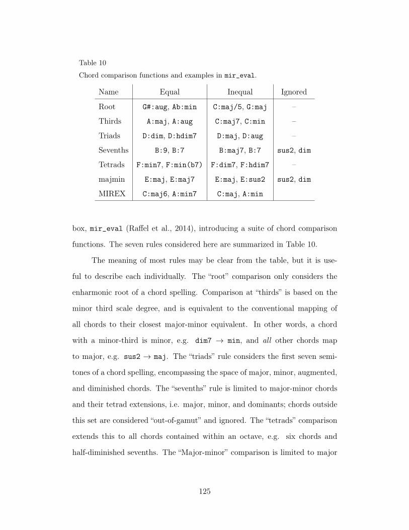
Table 10
Chord comparison functions and examples in mir_eval.
Name Equal Inequal Ignored
Root G#:aug, Ab:min C:maj/5, G:maj –
Thirds A:maj, A:aug C:maj7, C:min –
Triads D:dim, D:hdim7 D:maj, D:aug –
Sevenths B:9, B:7 B:maj7, B:7 sus2, dim
Tetrads F:min7, F:min(b7) F:dim7, F:hdim7 –
majmin E:maj, E:maj7 E:maj, E:sus2 sus2, dim
MIREX C:maj6, A:min7 C:maj, A:min
box, mir_eval (Raffel et al., 2014), introducing a suite of chord comparison
functions. The seven rules considered here are summarized in Table 10.
The meaning of most rules may be clear from the table, but it is use-
ful to describe each individually. The “root” comparison only considers the
enharmonic root of a chord spelling. Comparison at “thirds” is based on the
minor third scale degree, and is equivalent to the conventional mapping of
all chords to their closest major-minor equivalent. In other words, a chord
with a minor-third is minor, e.g. dim7 → min, and all other chords map
to major, e.g. sus2 → maj. The “triads” rule considers the first seven semi-
tones of a chord spelling, encompassing the space of major, minor, augmented,
and diminished chords. The “sevenths” rule is limited to major-minor chords
and their tetrad extensions, i.e. major, minor, and dominants; chords outside
this set are considered “out-of-gamut” and ignored. The “tetrads” comparison
extends this to all chords contained within an octave, e.g. six chords and
half-diminished sevenths. The “Major-minor” comparison is limited to major
125
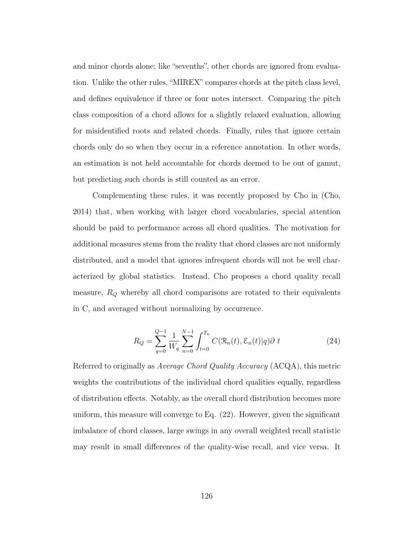
and minor chords alone; like “sevenths”, other chords are ignored from evalua-
tion. Unlike the other rules, “MIREX” compares chords at the pitch class level,
and defines equivalence if three or four notes intersect. Comparing the pitch
class composition of a chord allows for a slightly relaxed evaluation, allowing
for misidentified roots and related chords. Finally, rules that ignore certain
chords only do so when they occur in a reference annotation. In other words,
an estimation is not held accountable for chords deemed to be out of gamut,
but predicting such chords is still counted as an error.
Complementing these rules, it was recently proposed by Cho in (Cho,
2014) that, when working with larger chord vocabularies, special attention
should be paid to performance across all chord qualities. The motivation for
additional measures stems from the reality that chord classes are not uniformly
distributed, and a model that ignores infrequent chords will not be well char-
acterized by global statistics. Instead, Cho proposes a chord quality recall
measure, RQ whereby all chord comparisons are rotated to their equivalents
in C, and averaged without normalizing by occurrence.
RQ =
Q−1∑q=0
1
Wq
N−1∑n=0
∫ Tn
t=0
C(Rn(t),En(t)|q)∂ t (24)
Referred to originally as Average Chord Quality Accuracy (ACQA), this metric
weights the contributions of the individual chord qualities equally, regardless
of distribution effects. Notably, as the overall chord distribution becomes more
uniform, this measure will converge to Eq. (22). However, given the significant
imbalance of chord classes, large swings in any overall weighted recall statistic
may result in small differences of the quality-wise recall, and vice versa. It
126
should also be noted that the only comparison function on which quality-wise
recall is well defined is strict equivalence.
3 Pilot Study
Here, a preliminary study conducted by the author in 2012, and presented at
the International Conference of Machine Learning and Applications (ICMLA
2012), is revisited and expanded upon to frame subsequent work (Humphrey
& Bello, 2012). Approaching ACE from the perspective of classifying music
audio among the standard 24 Major-Minor classes, in addition to a no-chord
estimator, a deep convolutional network is explored as a means to realize a
full chord estimation system. Doing so not only addresses the questions of
relevance or quality toward chroma as a representation, but error analysis
of an end-to-end data-driven approach can be used to gain insight into the
data itself. This observation gives rise to two related questions: one, how
does performance change as a function of model complexity, and two, in what
instances can the model not overfit the training data?
3.1 Experimental Setup
Audio signals are downsampled to 7040Hz and transformed to a constant-Q
time-frequency representation. This transform consists of 36 bins per octave,
resulting in 252 filters spanning 27.5–1760Hz, and is applied at a framerate
of 40Hz. The high time-resolution of the constant-Q spectra is further re-
duced to a framerate of 4Hz by mean-filtering each frequency coefficient with
a 15-point window and decimating in time by a factor of 10. As discussed
previously, a constant-Q filterbank front-end provides the dual benefits of a
127
reduced input dimensionality, compared to the raw audio signal, and produces
a time-frequency representation that is linear in pitch, allowing for convolu-
tions to learn pitch-invariant features.
The input to the network is defined as a 20-frame time-frequency patch,
corresponding to 5 seconds. A long input duration is chosen in an effort
to learn context, thereby reducing the need for post-filtering. Local-contrast
normalization is applied to the constant-Q representation, serving as a form
of automatic gain control, and somewhat similar in principle to log-whitening
used previously in chord estimation (Cho et al., 2010). As an experimental
variable, data are augmented by applying random circular shifts along the
frequency axis during training within an octave range. The linearity of pitch
in a constant-Q representation affords the ability to “transpose” an observation
as if it were a chord of a different root by shifting the pitch tile and changing
the label accordingly. Every data point in the training set then contributes
to each chord class of the same quality (Major or minor), having the effect of
inflating the dataset by a factor of 12. The two conditions —before and after
augmentation— are referred to henceforth as “As-Is” and “Transposed”.
A five-layer 3D convolutional network is used as the general model, con-
sisting of three convolutional layers and two fully-connected layers. Six differ-
ent model complexities are explored by considering two high-level variables,
given in Table 11. The width of each layer, as the number of kernels or units,
increases over a small (S), medium (M), and large (L) configuration. Two
different kernel shapes are considered, referred to as 1 and 2. Note that only
the first convolutional layer makes use of pooling, and only in the frequency
dimension, by a factor of three in an effort to learn slight tuning invariance.
128
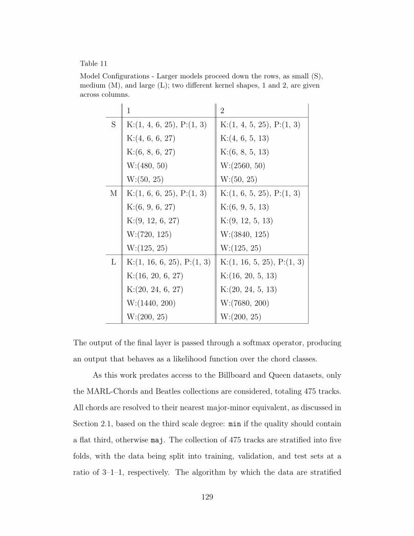
Table 11
Model Configurations - Larger models proceed down the rows, as small (S),medium (M), and large (L); two different kernel shapes, 1 and 2, are givenacross columns.
1 2
S K:(1, 4, 6, 25), P:(1, 3) K:(1, 4, 5, 25), P:(1, 3)
K:(4, 6, 6, 27) K:(4, 6, 5, 13)
K:(6, 8, 6, 27) K:(6, 8, 5, 13)
W:(480, 50) W:(2560, 50)
W:(50, 25) W:(50, 25)
M K:(1, 6, 6, 25), P:(1, 3) K:(1, 6, 5, 25), P:(1, 3)
K:(6, 9, 6, 27) K:(6, 9, 5, 13)
K:(9, 12, 6, 27) K:(9, 12, 5, 13)
W:(720, 125) W:(3840, 125)
W:(125, 25) W:(125, 25)
L K:(1, 16, 6, 25), P:(1, 3) K:(1, 16, 5, 25), P:(1, 3)
K:(16, 20, 6, 27) K:(16, 20, 5, 13)
K:(20, 24, 6, 27) K:(20, 24, 5, 13)
W:(1440, 200) W:(7680, 200)
W:(200, 25) W:(200, 25)
The output of the final layer is passed through a softmax operator, producing
an output that behaves as a likelihood function over the chord classes.
As this work predates access to the Billboard and Queen datasets, only
the MARL-Chords and Beatles collections are considered, totaling 475 tracks.
All chords are resolved to their nearest major-minor equivalent, as discussed in
Section 2.1, based on the third scale degree: min if the quality should contain
a flat third, otherwise maj. The collection of 475 tracks are stratified into five
folds, with the data being split into training, validation, and test sets at a
ratio of 3–1–1, respectively. The algorithm by which the data are stratified
129
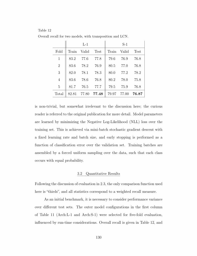
Table 12
Overall recall for two models, with transposition and LCN.
L-1 S-1
Fold Train Valid Test Train Valid Test
1 83.2 77.6 77.8 79.6 76.9 76.8
2 83.6 78.2 76.9 80.5 77.0 76.8
3 82.0 78.1 78.3 80.0 77.2 78.2
4 83.6 78.6 76.8 80.2 78.0 75.8
5 81.7 76.5 77.7 79.5 75.9 76.8
Total 82.81 77.80 77.48 79.97 77.00 76.87
is non-trivial, but somewhat irrelevant to the discussion here; the curious
reader is referred to the original publication for more detail. Model parameters
are learned by minimizing the Negative Log-Likelihood (NLL) loss over the
training set. This is achieved via mini-batch stochastic gradient descent with
a fixed learning rate and batch size, and early stopping is performed as a
function of classification error over the validation set. Training batches are
assembled by a forced uniform sampling over the data, such that each class
occurs with equal probability.
3.2 Quantitative Results
Following the discussion of evaluation in 2.3, the only comparison function used
here is “thirds”, and all statistics correspond to a weighted recall measure.
As an initial benchmark, it is necessary to consider performance variance
over different test sets. The outer model configurations in the first column
of Table 11 (Arch:L-1 and Arch:S-1) were selected for five-fold evaluation,
influenced by run-time considerations. Overall recall is given in Table 12, and
130
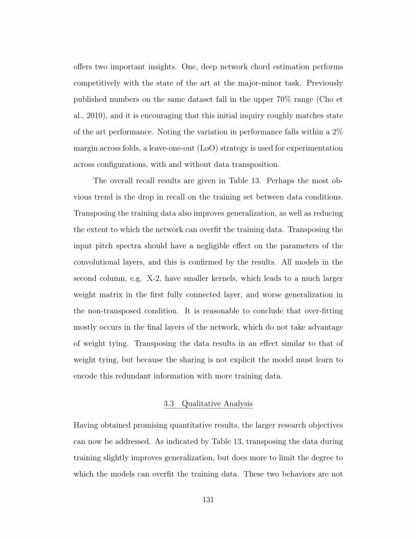
offers two important insights. One, deep network chord estimation performs
competitively with the state of the art at the major-minor task. Previously
published numbers on the same dataset fall in the upper 70% range (Cho et
al., 2010), and it is encouraging that this initial inquiry roughly matches state
of the art performance. Noting the variation in performance falls within a 2%
margin across folds, a leave-one-out (LoO) strategy is used for experimentation
across configurations, with and without data transposition.
The overall recall results are given in Table 13. Perhaps the most ob-
vious trend is the drop in recall on the training set between data conditions.
Transposing the training data also improves generalization, as well as reducing
the extent to which the network can overfit the training data. Transposing the
input pitch spectra should have a negligible effect on the parameters of the
convolutional layers, and this is confirmed by the results. All models in the
second column, e.g. X-2, have smaller kernels, which leads to a much larger
weight matrix in the first fully connected layer, and worse generalization in
the non-transposed condition. It is reasonable to conclude that over-fitting
mostly occurs in the final layers of the network, which do not take advantage
of weight tying. Transposing the data results in an effect similar to that of
weight tying, but because the sharing is not explicit the model must learn to
encode this redundant information with more training data.
3.3 Qualitative Analysis
Having obtained promising quantitative results, the larger research objectives
can now be addressed. As indicated by Table 13, transposing the data during
training slightly improves generalization, but does more to limit the degree to
which the models can overfit the training data. These two behaviors are not
131
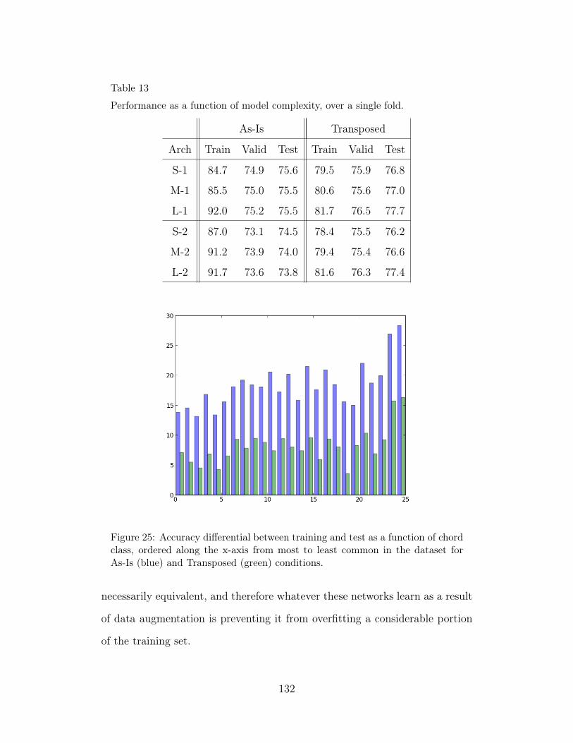
Table 13
Performance as a function of model complexity, over a single fold.
As-Is Transposed
Arch Train Valid Test Train Valid Test
S-1 84.7 74.9 75.6 79.5 75.9 76.8
M-1 85.5 75.0 75.5 80.6 75.6 77.0
L-1 92.0 75.2 75.5 81.7 76.5 77.7
S-2 87.0 73.1 74.5 78.4 75.5 76.2
M-2 91.2 73.9 74.0 79.4 75.4 76.6
L-2 91.7 73.6 73.8 81.6 76.3 77.4
Figure 25: Accuracy differential between training and test as a function of chordclass, ordered along the x-axis from most to least common in the dataset forAs-Is (blue) and Transposed (green) conditions.
necessarily equivalent, and therefore whatever these networks learn as a result
of data augmentation is preventing it from overfitting a considerable portion
of the training set.
132
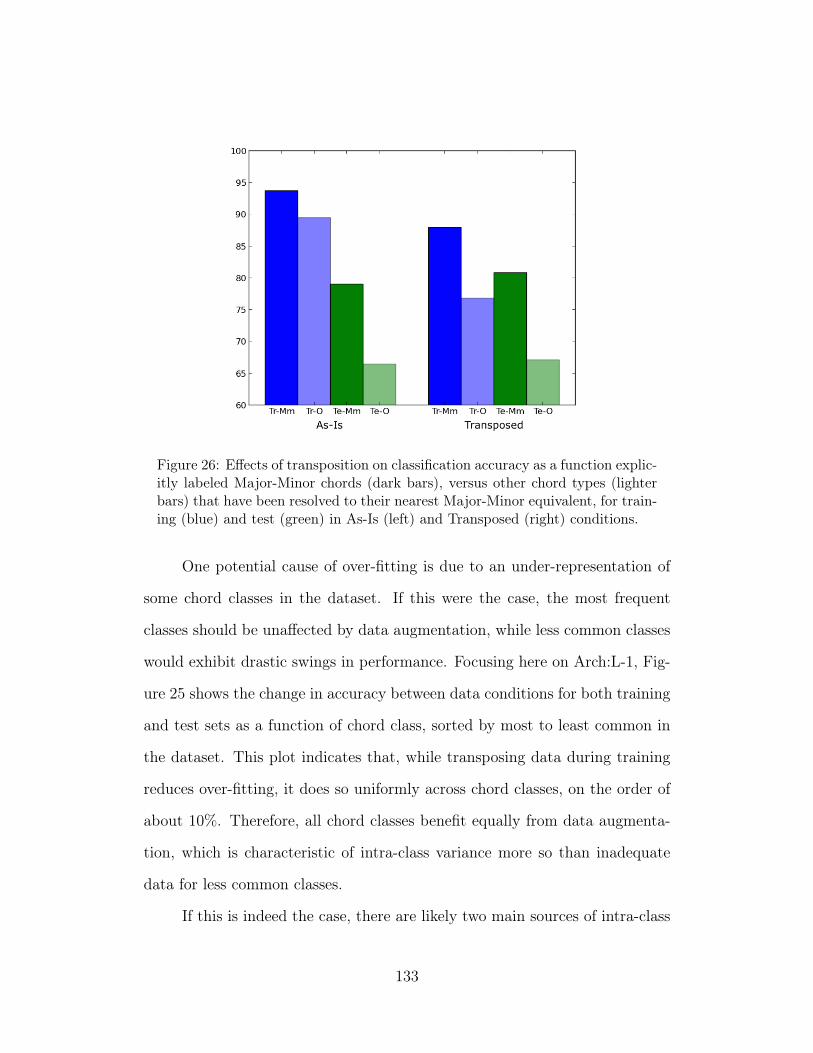
Figure 26: Effects of transposition on classification accuracy as a function explic-itly labeled Major-Minor chords (dark bars), versus other chord types (lighterbars) that have been resolved to their nearest Major-Minor equivalent, for train-ing (blue) and test (green) in As-Is (left) and Transposed (right) conditions.
One potential cause of over-fitting is due to an under-representation of
some chord classes in the dataset. If this were the case, the most frequent
classes should be unaffected by data augmentation, while less common classes
would exhibit drastic swings in performance. Focusing here on Arch:L-1, Fig-
ure 25 shows the change in accuracy between data conditions for both training
and test sets as a function of chord class, sorted by most to least common in
the dataset. This plot indicates that, while transposing data during training
reduces over-fitting, it does so uniformly across chord classes, on the order of
about 10%. Therefore, all chord classes benefit equally from data augmenta-
tion, which is characteristic of intra-class variance more so than inadequate
data for less common classes.
If this is indeed the case, there are likely two main sources of intra-class
133
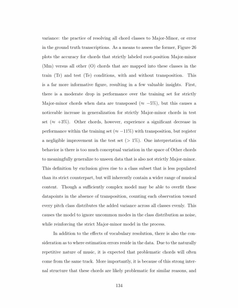
variance: the practice of resolving all chord classes to Major-Minor, or error
in the ground truth transcriptions. As a means to assess the former, Figure 26
plots the accuracy for chords that strictly labeled root-position Major-minor
(Mm) versus all other (O) chords that are mapped into these classes in the
train (Tr) and test (Te) conditions, with and without transposition. This
is a far more informative figure, resulting in a few valuable insights. First,
there is a moderate drop in performance over the training set for strictly
Major-minor chords when data are transposed (≈ −5%), but this causes a
noticeable increase in generalization for strictly Major-minor chords in test
set (≈ +3%). Other chords, however, experience a significant decrease in
performance within the training set (≈ −11%) with transposition, but register
a negligible improvement in the test set (> 1%). One interpretation of this
behavior is there is too much conceptual variation in the space of Other chords
to meaningfully generalize to unseen data that is also not strictly Major-minor.
This definition by exclusion gives rise to a class subset that is less populated
than its strict counterpart, but will inherently contain a wider range of musical
content. Though a sufficiently complex model may be able to overfit these
datapoints in the absence of transposition, counting each observation toward
every pitch class distributes the added variance across all classes evenly. This
causes the model to ignore uncommon modes in the class distribution as noise,
while reinforcing the strict Major-minor model in the process.
In addition to the effects of vocabulary resolution, there is also the con-
sideration as to where estimation errors reside in the data. Due to the naturally
repetitive nature of music, it is expected that problematic chords will often
come from the same track. More importantly, it is because of this strong inter-
nal structure that these chords are likely problematic for similar reasons, and
134
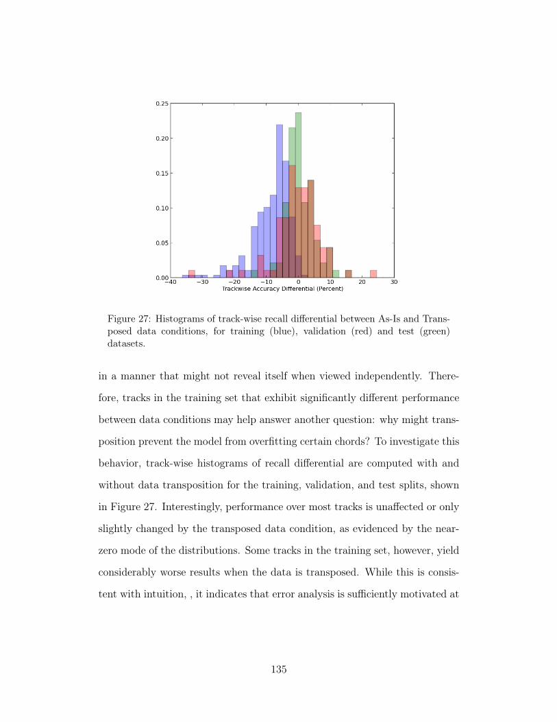
Figure 27: Histograms of track-wise recall differential between As-Is and Trans-posed data conditions, for training (blue), validation (red) and test (green)datasets.
in a manner that might not reveal itself when viewed independently. There-
fore, tracks in the training set that exhibit significantly different performance
between data conditions may help answer another question: why might trans-
position prevent the model from overfitting certain chords? To investigate this
behavior, track-wise histograms of recall differential are computed with and
without data transposition for the training, validation, and test splits, shown
in Figure 27. Interestingly, performance over most tracks is unaffected or only
slightly changed by the transposed data condition, as evidenced by the near-
zero mode of the distributions. Some tracks in the training set, however, yield
considerably worse results when the data is transposed. While this is consis-
tent with intuition, , it indicates that error analysis is sufficiently motivated at
135

the track, rather than instance, level, and may offer insight into future areas
of improvement.
One such problem track is “With or Without You” by U2. Here, the
ground truth transcription consists primarily of four chords: D:maj, D:maj/5,
D:maj6/6, and D:maj(4)/4. When resolved to the Major-minor vocabulary,
the transcription is reduced entirely to D:maj. In the As-Is data condition,
the model is able to call nearly the entire track D:maj; when training data
are transposed, however, the model is unable to reproduce the ground truth
transcription and instead tracks the bass motion, producing D:maj, A:maj,
B:min, and G:maj, a very common harmonic progression in popular music. As
far as quantitative evaluation is concerned, this second estimation exhibits a
high degree of mismatch with the reference transcription, but is qualitatively
reasonable and arguably far more useful to a musician. Importantly, this
illustrates that the process of mapping chords to a reduced vocabulary can
cause objective measures to deviate considerably from subjective experience,
and thus confounding evaluation.
However, perhaps even more critically, the reliability of the reference
annotation is somewhat dubious. Returning to the original song, one finds
reasonably ambiguous harmonic content, consisting of a vocal melody, the
moving bass line mentioned previously, a string pad sustaining a high-pitched
D, and a moving guitar riff. Therefore, as a point of comparison, an Internet
search yields six guitar chord transcriptions from the website Ultimate Gui-
tar∗. These alternative interpretations are consolidated in Table 14, alongside
the reference, noting both the average and number of ratings, as well as the
∗http://tabs.ultimate-guitar.com/u/u2/with_or_without_you_crd.htm, accessed 19April 2015.
136
number of views the tab has received. Though the view count is not directly
indicative of a transcription’s accuracy, it does provide a weak signal indicat-
ing that a large number of users did not rate it negatively. In considering this
particular example, there are a handful of takeaways to note. First, all but the
sixth of the user-generated chord transcriptions are equivalent by the conven-
tional major-minor mapping rules, which is, interestingly enough, the same one
produced by the model presented here. Second, this rather large community
of musicians shows, at least for this song, a strong preference for root position
chords. While it is difficult to determine why an annotator might choose one
interpretation than another, it would appear general, root-position chords are
preferred to nuanced chord spellings, e.g. G:maj over D:maj(4)/4. Finally,
this raises questions surrounding the practice of using such precise chord labels
for annotation. If nothing else, the flexibility afforded by this particular chord
syntax allows annotators to effectively “build” their own chords through non-
standard intervals or various bass intervals, amplifying the role subjectivity can
play in transcription. This is not only problematic from a practical standpoint
—are various annotators using this syntax consistently?— but atypical chord
spellings are most likely to appear when the music content being described is
especially ambiguous.
3.4 Conclusions
Following this initial inquiry, there are a few important conclusions to draw
that should influence subsequent work. First and foremost, the common prac-
tice of major-minor chord resolution is responsible for a significant amount of
error, both in training and test. While this approach simplifies the problem
being addressed, it appears to introduce uninformative variation to classes
137
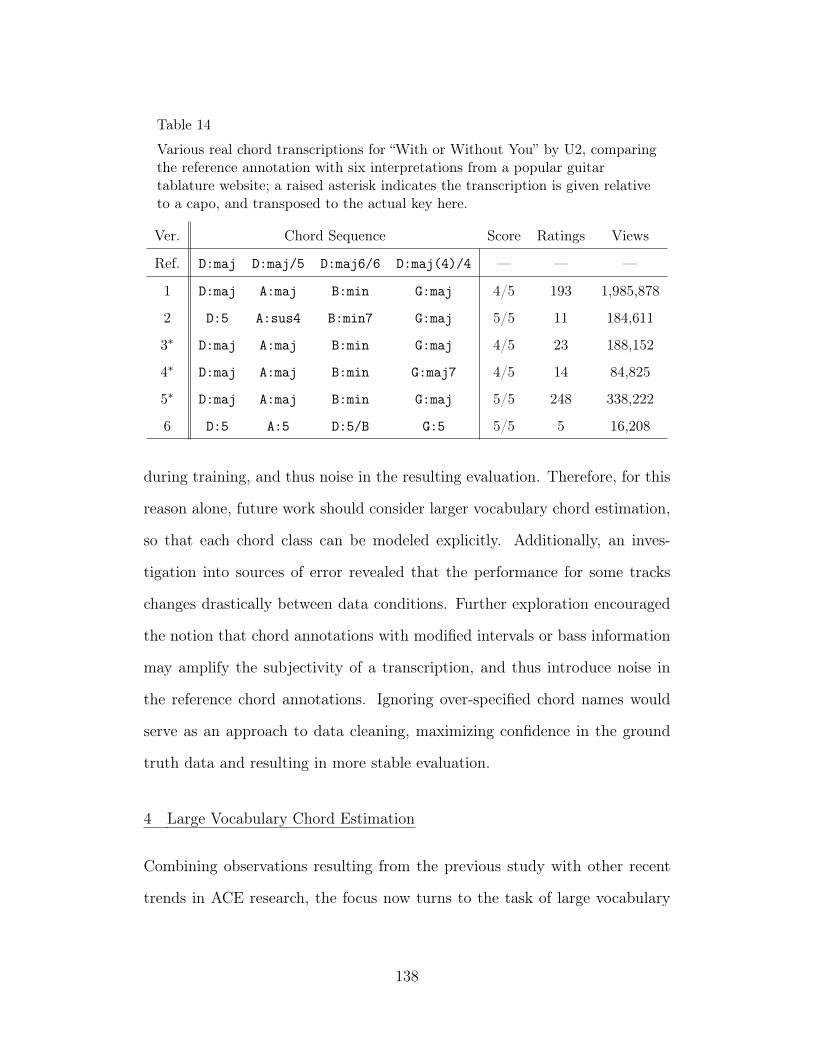
Table 14
Various real chord transcriptions for “With or Without You” by U2, comparingthe reference annotation with six interpretations from a popular guitartablature website; a raised asterisk indicates the transcription is given relativeto a capo, and transposed to the actual key here.
Ver. Chord Sequence Score Ratings Views
Ref. D:maj D:maj/5 D:maj6/6 D:maj(4)/4 — — —
1 D:maj A:maj B:min G:maj 4/5 193 1,985,878
2 D:5 A:sus4 B:min7 G:maj 5/5 11 184,611
3∗ D:maj A:maj B:min G:maj 4/5 23 188,152
4∗ D:maj A:maj B:min G:maj7 4/5 14 84,825
5∗ D:maj A:maj B:min G:maj 5/5 248 338,222
6 D:5 A:5 D:5/B G:5 5/5 5 16,208
during training, and thus noise in the resulting evaluation. Therefore, for this
reason alone, future work should consider larger vocabulary chord estimation,
so that each chord class can be modeled explicitly. Additionally, an inves-
tigation into sources of error revealed that the performance for some tracks
changes drastically between data conditions. Further exploration encouraged
the notion that chord annotations with modified intervals or bass information
may amplify the subjectivity of a transcription, and thus introduce noise in
the reference chord annotations. Ignoring over-specified chord names would
serve as an approach to data cleaning, maximizing confidence in the ground
truth data and resulting in more stable evaluation.
4 Large Vocabulary Chord Estimation
Combining observations resulting from the previous study with other recent
trends in ACE research, the focus now turns to the task of large vocabulary
138
ACE. There is a small body of research pertaining to vocabularies beyond the
major-minor formulation, exploring different mixtures of chord classes and in-
versions (Mauch & Dixon, 2010b; Ni, McVicar, Santos-Rodriguez, & De Bie,
2012). However, for the same reasons discussed in 2.1, comparing new en-
deavors to these efforts is problematic due to differences in the vocabularies
considered and data used. Perhaps the most advanced large-vocabulary ACE
systems to date is the recent work of Cho (Cho, 2014). The design of this
system is largely consistent with the previous overview of ACE research. A
multiband chroma representation is computed from beat-synchronous audio
analysis, producing four parallel chroma features. Each is modeled by a sep-
arate Gaussian Mixture Model, yielding four separate observation likelihoods
as a function of time. These four posteriors are then decoded jointly, using
a k-stream HMM, resulting in a time-aligned chord sequence. In addition to
being one of the highest performing systems at the recent iteration of MIReX,
a software implementation was obtained, thereby enabling direct comparisons
with this work. It also considers the largest vocabulary, and presents an even
greater challenge to the application of deep learning to ACE.
4.1 Data Considerations
Following the previous work of Cho (Cho, 2014), thirteen chord qualities, given
in Table 9, in all twelve pitch classes and one no-chord class are considered
here, for a total of 157 chord classes. Having all four datasets at hand, these
collections are merged into the largest collection of chord transcriptions used to
date, totaling 1235 tracks. Given that the collections were curated in isolation
of each other, it is a necessary first step to identify and remove duplicates to
avoid data contamination during cross validation. To these ends, each record-
139
ing is checked against the EchoNest Analyze API∗ and associated with its
track and song identifiers, corresponding to the recording and work, respec-
tively. Though multiple track IDs will map to the same song ID, uniqueness is
defined at the level of a song to ensure duplicates are removed. This identifies
18 redundant songs, and all but one is dropped for each collision from the total
collection, resulting in a final count of 1217 unique tracks.
Based on conclusions of the pilot study, the decision is made to ignore
all chord labels that do not strictly match one of the considered qualities,
i.e. chords that specify interval modifications, e.g. A:min(*b3), or non-root
inversions, e.g. C:maj/5. The motivation for doing so is two-fold. First, the
increased number of chord qualities makes it difficult to map certain chords
into one class or another, such as D:sus4(b7), which sits halfway between a
D:sus4 and a D:7. Second, cleaning the reference data on this criteria can
only improve annotation consistency; considering that the cumulative data is
compiled from multiple sources and several dozen annotators over the course
of a decade, it is quite unlikely that such nuanced conventions were used
identically by all subjects involved. This ignored subset comprises only a small
percentage of the overall data, and helps filter out suspicious chord spellings,
such as D:maj(1)/]1 or A:maj(2,∗3)/2.
Unsurprisingly, as the data is collected from real music, the distribu-
tion of absolute chord classes is extremely imbalanced. In fact, some chord
qualities do not occur in every root, and stratifying the data for training, vali-
dation, and testing only exacerbates the issue. Much previous work, including
the previous discussion, has demonstrated that chord names can be rotated
∗http://developer.echonest.com/docs/v4
140
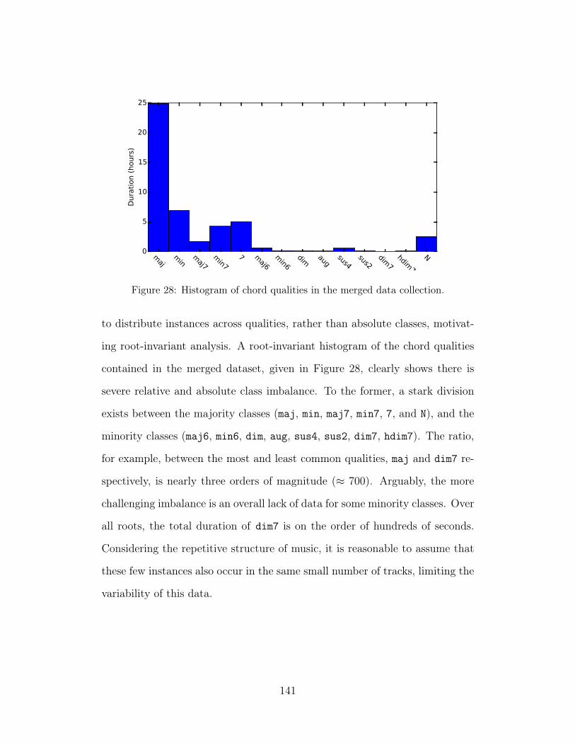
maj
min
maj7
min7
7 maj6
min6
dimaug
sus4sus2
dim7
hdim7
N0
5
10
15
20
25
Dura
tion (
hours
)
Figure 28: Histogram of chord qualities in the merged data collection.
to distribute instances across qualities, rather than absolute classes, motivat-
ing root-invariant analysis. A root-invariant histogram of the chord qualities
contained in the merged dataset, given in Figure 28, clearly shows there is
severe relative and absolute class imbalance. To the former, a stark division
exists between the majority classes (maj, min, maj7, min7, 7, and N), and the
minority classes (maj6, min6, dim, aug, sus4, sus2, dim7, hdim7). The ratio,
for example, between the most and least common qualities, maj and dim7 re-
spectively, is nearly three orders of magnitude (≈ 700). Arguably, the more
challenging imbalance is an overall lack of data for some minority classes. Over
all roots, the total duration of dim7 is on the order of hundreds of seconds.
Considering the repetitive structure of music, it is reasonable to assume that
these few instances also occur in the same small number of tracks, limiting the
variability of this data.
141
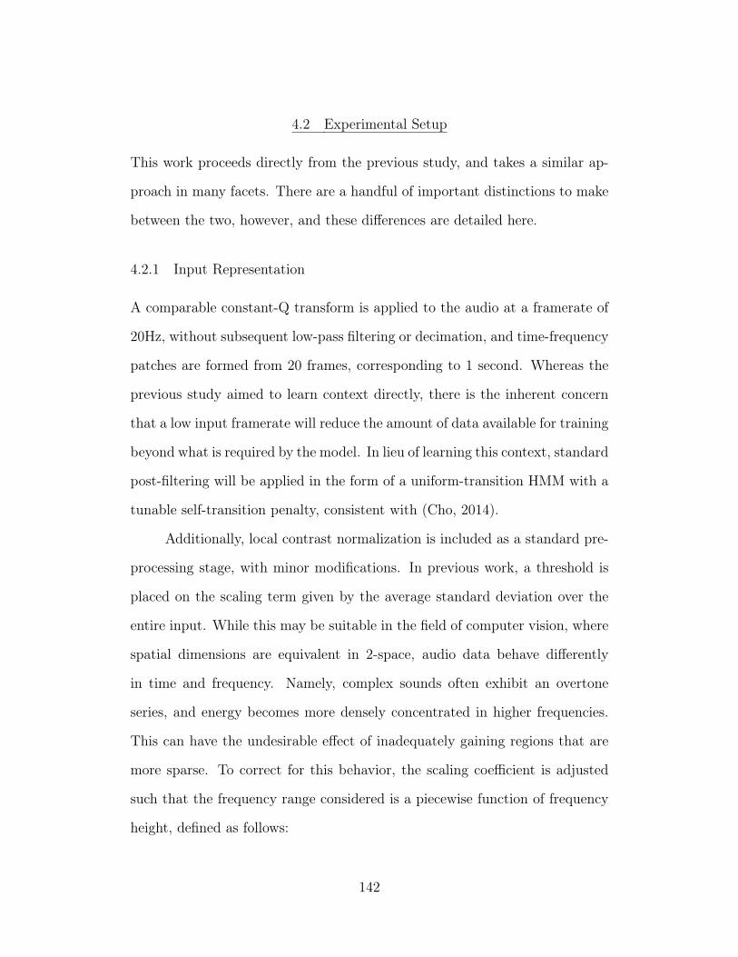
4.2 Experimental Setup
This work proceeds directly from the previous study, and takes a similar ap-
proach in many facets. There are a handful of important distinctions to make
between the two, however, and these differences are detailed here.
4.2.1 Input Representation
A comparable constant-Q transform is applied to the audio at a framerate of
20Hz, without subsequent low-pass filtering or decimation, and time-frequency
patches are formed from 20 frames, corresponding to 1 second. Whereas the
previous study aimed to learn context directly, there is the inherent concern
that a low input framerate will reduce the amount of data available for training
beyond what is required by the model. In lieu of learning this context, standard
post-filtering will be applied in the form of a uniform-transition HMM with a
tunable self-transition penalty, consistent with (Cho, 2014).
Additionally, local contrast normalization is included as a standard pre-
processing stage, with minor modifications. In previous work, a threshold is
placed on the scaling term given by the average standard deviation over the
entire input. While this may be suitable in the field of computer vision, where
spatial dimensions are equivalent in 2-space, audio data behave differently
in time and frequency. Namely, complex sounds often exhibit an overtone
series, and energy becomes more densely concentrated in higher frequencies.
This can have the undesirable effect of inadequately gaining regions that are
more sparse. To correct for this behavior, the scaling coefficient is adjusted
such that the frequency range considered is a piecewise function of frequency
height, defined as follows:
142
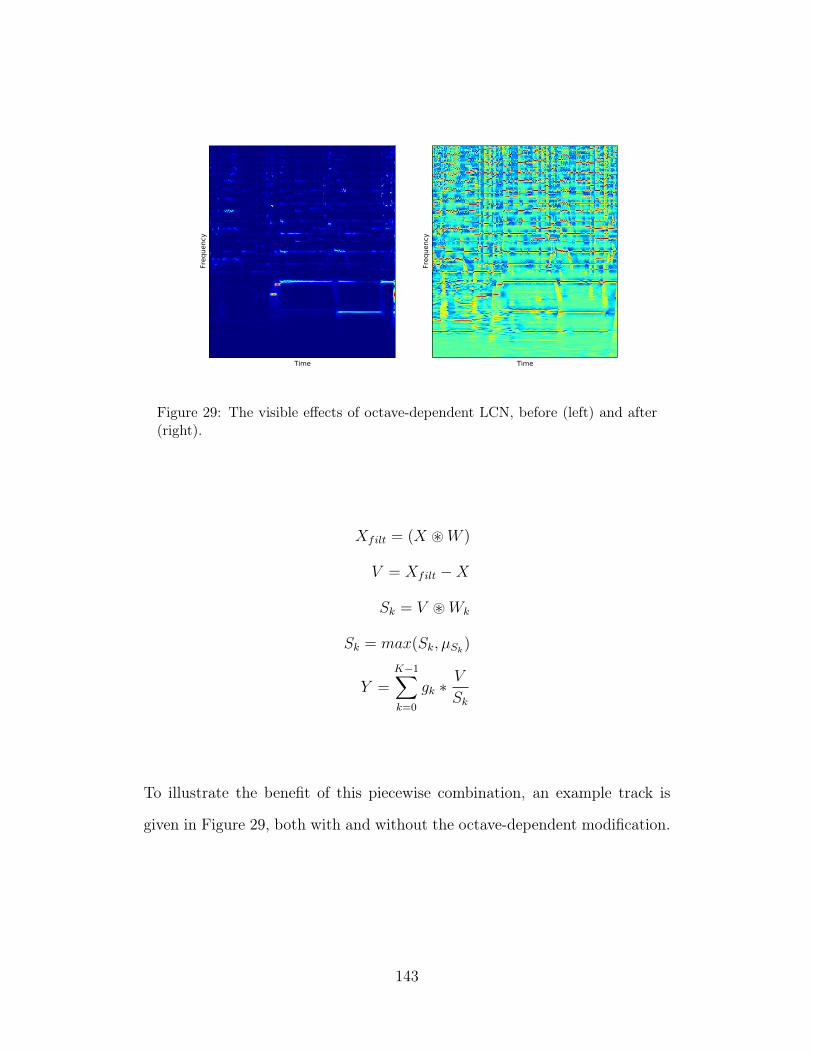
Time
Frequency
Time
Frequency
Figure 29: The visible effects of octave-dependent LCN, before (left) and after(right).
Xfilt = (X ~W )
V = Xfilt −X
Sk = V ~Wk
Sk = max(Sk, µSk)
Y =K−1∑k=0
gk ∗V
Sk
To illustrate the benefit of this piecewise combination, an example track is
given in Figure 29, both with and without the octave-dependent modification.
143
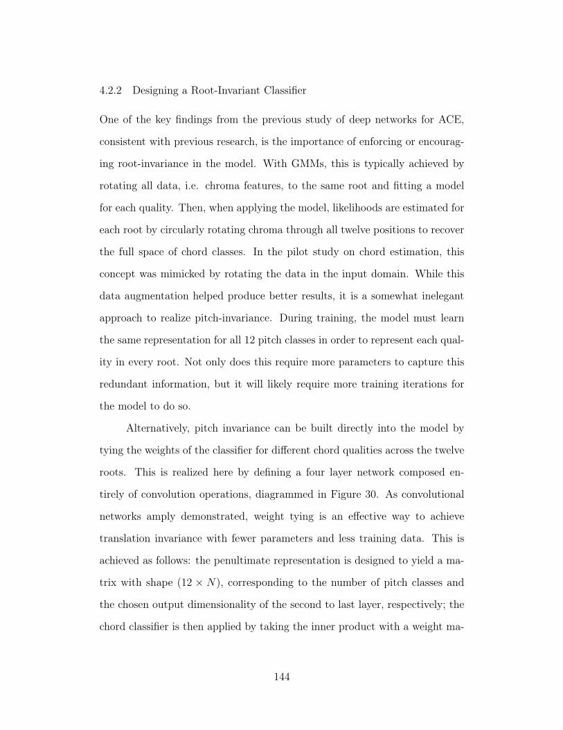
4.2.2 Designing a Root-Invariant Classifier
One of the key findings from the previous study of deep networks for ACE,
consistent with previous research, is the importance of enforcing or encourag-
ing root-invariance in the model. With GMMs, this is typically achieved by
rotating all data, i.e. chroma features, to the same root and fitting a model
for each quality. Then, when applying the model, likelihoods are estimated for
each root by circularly rotating chroma through all twelve positions to recover
the full space of chord classes. In the pilot study on chord estimation, this
concept was mimicked by rotating the data in the input domain. While this
data augmentation helped produce better results, it is a somewhat inelegant
approach to realize pitch-invariance. During training, the model must learn
the same representation for all 12 pitch classes in order to represent each qual-
ity in every root. Not only does this require more parameters to capture this
redundant information, but it will likely require more training iterations for
the model to do so.
Alternatively, pitch invariance can be built directly into the model by
tying the weights of the classifier for different chord qualities across the twelve
roots. This is realized here by defining a four layer network composed en-
tirely of convolution operations, diagrammed in Figure 30. As convolutional
networks amply demonstrated, weight tying is an effective way to achieve
translation invariance with fewer parameters and less training data. This is
achieved as follows: the penultimate representation is designed to yield a ma-
trix with shape (12 × N), corresponding to the number of pitch classes and
the chosen output dimensionality of the second to last layer, respectively; the
chord classifier is then applied by taking the inner product with a weight ma-
144
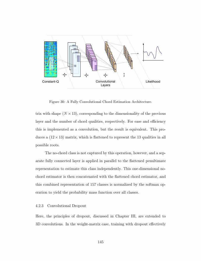
ConvolutionalLayers
Constant-Q Likelihood
Figure 30: A Fully Convolutional Chord Estimation Architecture.
trix with shape (N × 13), corresponding to the dimensionality of the previous
layer and the number of chord qualities, respectively. For ease and efficiency
this is implemented as a convolution, but the result is equivalent. This pro-
duces a (12× 13) matrix, which is flattened to represent the 13 qualities in all
possible roots.
The no-chord class is not captured by this operation, however, and a sep-
arate fully connected layer is applied in parallel to the flattened penultimate
representation to estimate this class independently. This one-dimensional no-
chord estimator is then concatenated with the flattened chord estimator, and
this combined representation of 157 classes is normalized by the softmax op-
eration to yield the probability mass function over all classes.
4.2.3 Convolutional Dropout
Here, the principles of dropout, discussed in Chapter III, are extended to
3D convolutions. In the weight-matrix case, training with dropout effectively
145
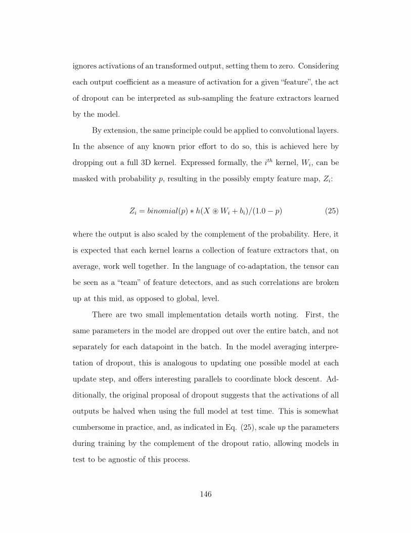
ignores activations of an transformed output, setting them to zero. Considering
each output coefficient as a measure of activation for a given “feature”, the act
of dropout can be interpreted as sub-sampling the feature extractors learned
by the model.
By extension, the same principle could be applied to convolutional layers.
In the absence of any known prior effort to do so, this is achieved here by
dropping out a full 3D kernel. Expressed formally, the ith kernel, Wi, can be
masked with probability p, resulting in the possibly empty feature map, Zi:
Zi = binomial(p) ∗ h(X ~Wi + bi)/(1.0− p) (25)
where the output is also scaled by the complement of the probability. Here, it
is expected that each kernel learns a collection of feature extractors that, on
average, work well together. In the language of co-adaptation, the tensor can
be seen as a “team” of feature detectors, and as such correlations are broken
up at this mid, as opposed to global, level.
There are two small implementation details worth noting. First, the
same parameters in the model are dropped out over the entire batch, and not
separately for each datapoint in the batch. In the model averaging interpre-
tation of dropout, this is analogous to updating one possible model at each
update step, and offers interesting parallels to coordinate block descent. Ad-
ditionally, the original proposal of dropout suggests that the activations of all
outputs be halved when using the full model at test time. This is somewhat
cumbersome in practice, and, as indicated in Eq. (25), scale up the parameters
during training by the complement of the dropout ratio, allowing models in
test to be agnostic of this process.
146
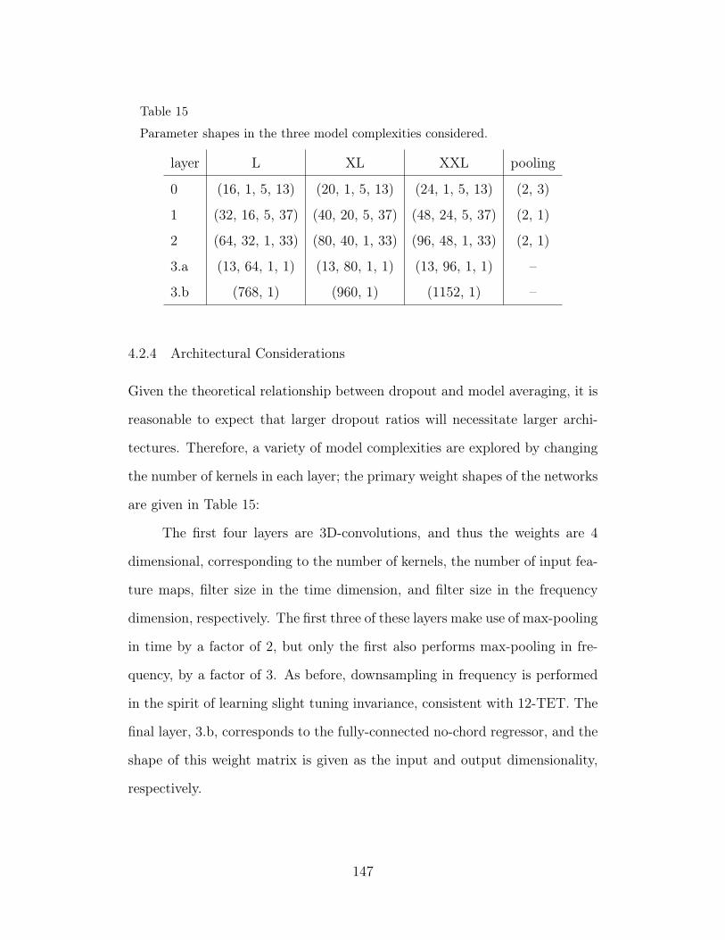
Table 15
Parameter shapes in the three model complexities considered.
layer L XL XXL pooling
0 (16, 1, 5, 13) (20, 1, 5, 13) (24, 1, 5, 13) (2, 3)
1 (32, 16, 5, 37) (40, 20, 5, 37) (48, 24, 5, 37) (2, 1)
2 (64, 32, 1, 33) (80, 40, 1, 33) (96, 48, 1, 33) (2, 1)
3.a (13, 64, 1, 1) (13, 80, 1, 1) (13, 96, 1, 1) –
3.b (768, 1) (960, 1) (1152, 1) –
4.2.4 Architectural Considerations
Given the theoretical relationship between dropout and model averaging, it is
reasonable to expect that larger dropout ratios will necessitate larger archi-
tectures. Therefore, a variety of model complexities are explored by changing
the number of kernels in each layer; the primary weight shapes of the networks
are given in Table 15:
The first four layers are 3D-convolutions, and thus the weights are 4
dimensional, corresponding to the number of kernels, the number of input fea-
ture maps, filter size in the time dimension, and filter size in the frequency
dimension, respectively. The first three of these layers make use of max-pooling
in time by a factor of 2, but only the first also performs max-pooling in fre-
quency, by a factor of 3. As before, downsampling in frequency is performed
in the spirit of learning slight tuning invariance, consistent with 12-TET. The
final layer, 3.b, corresponds to the fully-connected no-chord regressor, and the
shape of this weight matrix is given as the input and output dimensionality,
respectively.
147
4.2.5 Correcting Class Imbalance with Scaled Likelihood Estimation
Having defined the output of the model as a probability function, it is straight-
forward to again optimize the parameters to the negative log-likelihood over
the dataset. However, there are two difficulties that prohibit the uniform pre-
sentation of classes, as in previous work. First, due to the increased number of
classes, mini-batches would either need to consist of many datapoints, increas-
ing the processing time of each batch, or the learning rate would need to be
smaller or diminishing over time to prevent oscillation, increasing the number
of iterations necessary to converge. To the latter point, it is easy to imagine
scenarios where gradient descent wobbles back and forth between updates, as
each batch pulls the parameters in a slightly different direction. The other
challenge this raises is a result of the considerable class imbalance, where uni-
form presentation would both spend too much time on minority classes and
inhibit the speed at which the model could learn the full extent of the majority
classes.
The solution to this problem is found in Bayes’ theorem, where the net-
work is understood as yielding a class posterior probability, P (Y |x), for the
chord class, Y , given the observation, x:
P (x|Y ) =P (Y |x)P (x)
P (Y )(26)
The observation likelihood, P (x|Y ), is then a function of the posterior,
the class prior, P (Y ), and probability of the observation itself, P (x). This
final quantity is independent and thus can be ignored:
P (x|Y ) ∝P (Y |x)
P (Y )(27)
148

While the deep network is trained to produce the class posterior, the
class prior can be measured empirically over the training set, and divided out
after the fact. Referred to as scaled likelihood estimation, this strategy has
proven effective at reducing the effects of class imbalances in the functionally
related domain of automatic speech recognition (Dahl, Yu, Deng, & Acero,
2012). Notably, scaled likelihood estimation is particularly attractive here
because it scales well with the number of estimated classes.
As a final comment, a possible pitfall when applying likelihood scaling
is a matter of numerical stability arising from the least represented classes, or
classes that might not even occur in the training set. Whereas this can be
mitigated with pseudo-counting —setting a heuristically determined, non-zero
lower bound— the class prior here is computed by counting each observation
toward the same quality in all roots. Though this prior could be seen as
a coefficient vector to optimize in a more direct way, this approach works
reasonably well in practice.
4.2.6 Training and Early Stopping
In contrast to the previous study, which converged to a stable result in a few
thousand iterations, it takes considerably more effort to train models for this
task, on the order of hundreds of thousands of iterations. Given the lengthy run
time, parameters are saved every 1k iterations during training, and frame the
problem of early stopping as a brute-force search over a finite set of parameter
configurations. Due to the application of Viterbi and the coupling with the
self transition penalty, validation is non-trivial and computationally expensive.
Therefore, exhaustive validation is performed every 10k iterations, starting
at 5k. The best model and self-transition penalty are chosen by finding the
149
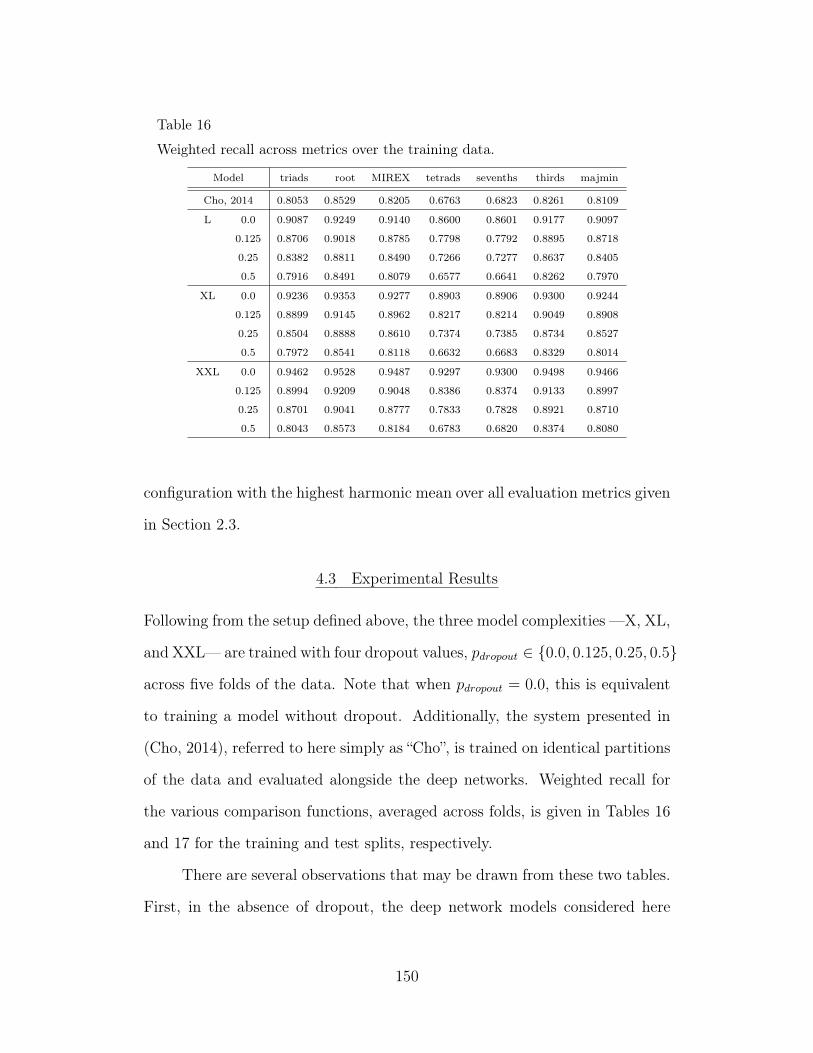
Table 16
Weighted recall across metrics over the training data.
Model triads root MIREX tetrads sevenths thirds majmin
Cho, 2014 0.8053 0.8529 0.8205 0.6763 0.6823 0.8261 0.8109
L 0.0 0.9087 0.9249 0.9140 0.8600 0.8601 0.9177 0.9097
0.125 0.8706 0.9018 0.8785 0.7798 0.7792 0.8895 0.8718
0.25 0.8382 0.8811 0.8490 0.7266 0.7277 0.8637 0.8405
0.5 0.7916 0.8491 0.8079 0.6577 0.6641 0.8262 0.7970
XL 0.0 0.9236 0.9353 0.9277 0.8903 0.8906 0.9300 0.9244
0.125 0.8899 0.9145 0.8962 0.8217 0.8214 0.9049 0.8908
0.25 0.8504 0.8888 0.8610 0.7374 0.7385 0.8734 0.8527
0.5 0.7972 0.8541 0.8118 0.6632 0.6683 0.8329 0.8014
XXL 0.0 0.9462 0.9528 0.9487 0.9297 0.9300 0.9498 0.9466
0.125 0.8994 0.9209 0.9048 0.8386 0.8374 0.9133 0.8997
0.25 0.8701 0.9041 0.8777 0.7833 0.7828 0.8921 0.8710
0.5 0.8043 0.8573 0.8184 0.6783 0.6820 0.8374 0.8080
configuration with the highest harmonic mean over all evaluation metrics given
in Section 2.3.
4.3 Experimental Results
Following from the setup defined above, the three model complexities —X, XL,
and XXL— are trained with four dropout values, pdropout ∈ {0.0, 0.125, 0.25, 0.5}
across five folds of the data. Note that when pdropout = 0.0, this is equivalent
to training a model without dropout. Additionally, the system presented in
(Cho, 2014), referred to here simply as “Cho”, is trained on identical partitions
of the data and evaluated alongside the deep networks. Weighted recall for
the various comparison functions, averaged across folds, is given in Tables 16
and 17 for the training and test splits, respectively.
There are several observations that may be drawn from these two tables.
First, in the absence of dropout, the deep network models considered here
150
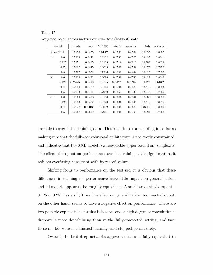
Table 17
Weighted recall across metrics over the test (holdout) data.
Model triads root MIREX tetrads sevenths thirds majmin
Cho, 2014 0.7970 0.8475 0.8147 0.6592 0.6704 0.8197 0.8057
L 0.0 0.7939 0.8442 0.8102 0.6583 0.6725 0.8135 0.8041
0.125 0.7951 0.8465 0.8109 0.6516 0.6616 0.8203 0.8028
0.25 0.7882 0.8445 0.8039 0.6509 0.6592 0.8175 0.7950
0.5 0.7762 0.8372 0.7936 0.6358 0.6442 0.8115 0.7832
XL 0.0 0.7939 0.8432 0.8098 0.6589 0.6736 0.8122 0.8042
0.125 0.7995 0.8493 0.8145 0.6673 0.6788 0.8227 0.8077
0.25 0.7950 0.8479 0.8114 0.6493 0.6580 0.8215 0.8023
0.5 0.7773 0.8401 0.7940 0.6351 0.6430 0.8147 0.7836
XXL 0.0 0.7969 0.8463 0.8130 0.6583 0.6741 0.8136 0.8080
0.125 0.7993 0.8477 0.8140 0.6633 0.6745 0.8215 0.8075
0.25 0.7947 0.8497 0.8092 0.6592 0.6686 0.8241 0.8020
0.5 0.7768 0.8369 0.7941 0.6392 0.6468 0.8121 0.7830
are able to overfit the training data. This is an important finding in so far as
making sure that the fully-convolutional architecture is not overly constrained,
and indicates that the XXL model is a reasonable upper bound on complexity.
The effect of dropout on performance over the training set is significant, as it
reduces overfitting consistent with increased values.
Shifting focus to performance on the test set, it is obvious that these
differences in training set performance have little impact on generalization,
and all models appear to be roughly equivalent. A small amount of dropout –
0.125 or 0.25– has a slight positive effect on generalization; too much dropout,
on the other hand, seems to have a negative effect on performance. There are
two possible explanations for this behavior: one, a high degree of convolutional
dropout is more destabilizing than in the fully-connected setting; and two,
these models were not finished learning, and stopped prematurely.
Overall, the best deep networks appear to be essentially equivalent to
151
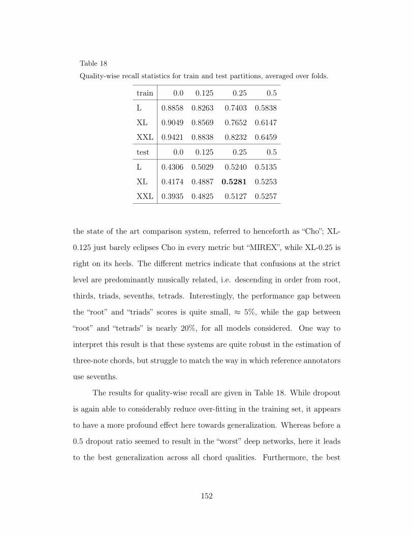
Table 18
Quality-wise recall statistics for train and test partitions, averaged over folds.
train 0.0 0.125 0.25 0.5
L 0.8858 0.8263 0.7403 0.5838
XL 0.9049 0.8569 0.7652 0.6147
XXL 0.9421 0.8838 0.8232 0.6459
test 0.0 0.125 0.25 0.5
L 0.4306 0.5029 0.5240 0.5135
XL 0.4174 0.4887 0.5281 0.5253
XXL 0.3935 0.4825 0.5127 0.5257
the state of the art comparison system, referred to henceforth as “Cho”; XL-
0.125 just barely eclipses Cho in every metric but “MIREX”, while XL-0.25 is
right on its heels. The different metrics indicate that confusions at the strict
level are predominantly musically related, i.e. descending in order from root,
thirds, triads, sevenths, tetrads. Interestingly, the performance gap between
the “root” and “triads” scores is quite small, ≈ 5%, while the gap between
“root” and “tetrads” is nearly 20%, for all models considered. One way to
interpret this result is that these systems are quite robust in the estimation of
three-note chords, but struggle to match the way in which reference annotators
use sevenths.
The results for quality-wise recall are given in Table 18. While dropout
is again able to considerably reduce over-fitting in the training set, it appears
to have a more profound effect here towards generalization. Whereas before a
0.5 dropout ratio seemed to result in the “worst” deep networks, here it leads
to the best generalization across all chord qualities. Furthermore, the best
152
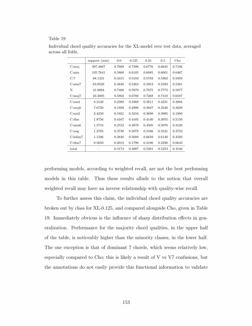
Table 19
Individual chord quality accuracies for the XL-model over test data, averagedacross all folds.
support (min) 0.0 0.125 0.25 0.5 Cho
C:maj 397.4887 0.7669 0.7390 0.6776 0.6645 0.7196
C:min 105.7641 0.5868 0.6105 0.6085 0.6001 0.6467
C:7 68.1321 0.4315 0.5183 0.5783 0.5362 0.5959
C:min7 63.9526 0.4840 0.5263 0.5954 0.5593 0.5381
N 41.6994 0.7408 0.7679 0.7875 0.7772 0.5877
C:maj7 23.3095 0.5802 0.6780 0.7268 0.7410 0.6587
C:sus4 8.3140 0.2380 0.3369 0.3811 0.4231 0.3894
C:maj6 7.6729 0.1929 0.2908 0.3847 0.3540 0.3028
C:sus2 2.4250 0.1921 0.3216 0.3698 0.3995 0.1993
C:dim 1.8756 0.4167 0.4105 0.4140 0.3955 0.5150
C:min6 1.5716 0.2552 0.3870 0.4505 0.5076 0.3129
C:aug 1.2705 0.3730 0.5078 0.5346 0.5521 0.3752
C:hdim7 1.1506 0.3840 0.5688 0.6659 0.6140 0.4593
C:dim7 0.5650 0.2012 0.1790 0.2186 0.2296 0.0643
total – 0.4174 0.4887 0.5281 0.5253 0.4546
performing models, according to weighted recall, are not the best performing
models in this table. Thus these results allude to the notion that overall
weighted recall may have an inverse relationship with quality-wise recall.
To further assess this claim, the individual chord quality accuracies are
broken out by class for XL-0.125, and compared alongside Cho, given in Table
19. Immediately obvious is the influence of sharp distribution effects in gen-
eralization. Performance for the majority chord qualities, in the upper half
of the table, is noticeably higher than the minority classes, in the lower half.
The one exception is that of dominant 7 chords, which seems relatively low,
especially compared to Cho; this is likely a result of V vs V7 confusions, but
the annotations do not easily provide this functional information to validate
153
the hypothesis∗. XXL-0.25 yields near identical weighted recall statistics to
Cho, but achieves a significant increase in quality-wise recall, RQ, 0.5127 to
0.4546 (δ0.0581).
Notably, the only chord quality to decrease in accuracy with dropout is
major, indicating that, with the addition of dropout, the decision boundary
between major and its related classes, e.g. major 7 and dominant 7, shift.
However, because of the significant imbalance in the support of each quality,
given here in minutes, a small drop in accuracy for major yields a consider-
able drop in weighted recall overall. To illustrate, between the 0.125 and 0.25
dropout ratios, major accuracy drops 6%, while dominant 7 and major 7 ac-
curacy increase 6% and 5%, respectively. In terms of overall time though, this
comes at the expense of 24 minutes of major now being classified “incorrectly”,
compared to a combined 5 minutes of dominant and major 7’s now being “cor-
rect”. Therefore, it seems there is a trade-off between these two measures, and
thus the representational power of the model does not really change. Rather,
the decision boundaries between overlapping classes must prefer one over the
other, and thus model selection may ultimately be a function of use-case. For
example, is it better to have a model that predicts simpler chords, i.e. major,
most of the time? Or to have a model that makes use of a wider vocabulary of
chords? Lastly, it is necessary to recognize that, while quality-wise recall pro-
vides a glimpse into more nuanced system behavior, the severe class imbalance
results in a rather volatile metric.
As a final investigation of algorithm performance with this particular
collection of data, having the estimations of two very different computational
∗The Billboard dataset does provide tonic information, and thus this relationship could berecovered from the data; however, it is left here as a fertile area for future work
154
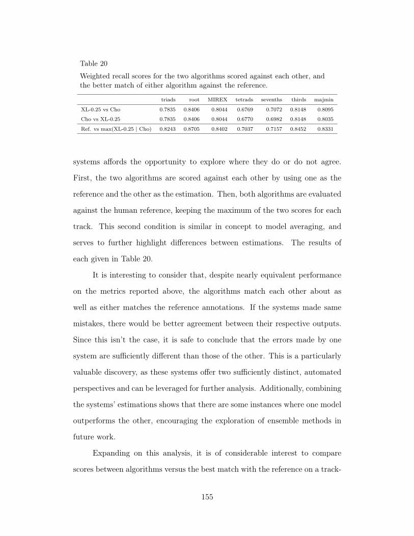
Table 20
Weighted recall scores for the two algorithms scored against each other, andthe better match of either algorithm against the reference.
triads root MIREX tetrads sevenths thirds majmin
XL-0.25 vs Cho 0.7835 0.8406 0.8044 0.6769 0.7072 0.8148 0.8095
Cho vs XL-0.25 0.7835 0.8406 0.8044 0.6770 0.6982 0.8148 0.8035
Ref. vs max(XL-0.25 | Cho) 0.8243 0.8705 0.8402 0.7037 0.7157 0.8452 0.8331
systems affords the opportunity to explore where they do or do not agree.
First, the two algorithms are scored against each other by using one as the
reference and the other as the estimation. Then, both algorithms are evaluated
against the human reference, keeping the maximum of the two scores for each
track. This second condition is similar in concept to model averaging, and
serves to further highlight differences between estimations. The results of
each given in Table 20.
It is interesting to consider that, despite nearly equivalent performance
on the metrics reported above, the algorithms match each other about as
well as either matches the reference annotations. If the systems made same
mistakes, there would be better agreement between their respective outputs.
Since this isn’t the case, it is safe to conclude that the errors made by one
system are sufficiently different than those of the other. This is a particularly
valuable discovery, as these systems offer two sufficiently distinct, automated
perspectives and can be leveraged for further analysis. Additionally, combining
the systems’ estimations shows that there are some instances where one model
outperforms the other, encouraging the exploration of ensemble methods in
future work.
Expanding on this analysis, it is of considerable interest to compare
scores between algorithms versus the best match with the reference on a track-
155
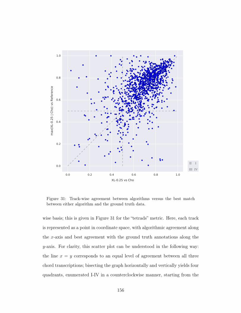
III
III IV
Figure 31: Track-wise agreement between algorithms versus the best matchbetween either algorithm and the ground truth data.
wise basis; this is given in Figure 31 for the “tetrads” metric. Here, each track
is represented as a point in coordinate space, with algorithmic agreement along
the x-axis and best agreement with the ground truth annotations along the
y-axis. For clarity, this scatter plot can be understood in the following way:
the line x = y corresponds to an equal level of agreement between all three
chord transcriptions; bisecting the graph horizontally and vertically yields four
quadrants, enumerated I-IV in a counterclockwise manner, starting from the
156
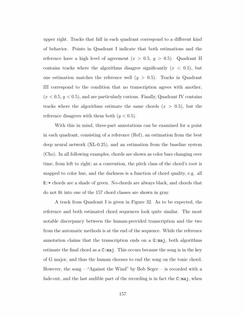
upper right. Tracks that fall in each quadrant correspond to a different kind
of behavior. Points in Quadrant I indicate that both estimations and the
reference have a high level of agreement (x > 0.5, y > 0.5). Quadrant II
contains tracks where the algorithms disagree significantly (x < 0.5), but
one estimation matches the reference well (y > 0.5). Tracks in Quadrant
III correspond to the condition that no transcription agrees with another,
(x < 0.5, y < 0.5), and are particularly curious. Finally, Quadrant IV contains
tracks where the algorithms estimate the same chords (x > 0.5), but the
reference disagrees with them both (y < 0.5).
With this in mind, three-part annotations can be examined for a point
in each quadrant, consisting of a reference (Ref), an estimation from the best
deep neural network (XL-0.25), and an estimation from the baseline system
(Cho). In all following examples, chords are shown as color bars changing over
time, from left to right; as a convention, the pitch class of the chord’s root is
mapped to color hue, and the darkness is a function of chord quality, e.g. all
E:* chords are a shade of green. No-chords are always black, and chords that
do not fit into one of the 157 chord classes are shown in gray.
A track from Quadrant I is given in Figure 32. As to be expected, the
reference and both estimated chord sequences look quite similar. The most
notable discrepancy between the human-provided transcription and the two
from the automatic methods is at the end of the sequence. While the reference
annotation claims that the transcription ends on a G:maj, both algorithms
estimate the final chord as a C:maj. This occurs because the song is in the key
of G major, and thus the human chooses to end the song on the tonic chord.
However, the song —“Against the Wind” by Bob Seger— is recorded with a
fade-out, and the last audible part of the recording is in fact the C:maj, when
157
Ref.
XL-
0.2
5
Time
Cho
G:maj C:maj B:min D:maj E:min N C:maj7 A:min A:min7 C:maj6
Figure 32: Reference and estimated chord sequences for a track in Quadrant I,where both algorithms agree with the reference.
playback volume is adjusted accordingly. Therefore, this is an instance of the
automatic systems being more precise than the human annotator.
Next, a track from Quadrant II —“Smoking Gun” by Robert Cray—
is considered in Figure 33. While the baseline system, Cho, agrees strongly
with the reference that the predominant chord is an E:min7, the deep net-
work, XL-0.25, prefers E:min, and produces a poor “tetrads” score as a result.
This confusion is an understandable one, and highlights an interesting issue in
automatic chord estimation evaluation. Depending on the instance, it could
be argued that some chords are not fundamentally different classes, and thus
“confusions” in the traditional machine learning sense, but rather a subset
of a more specified chord, e.g. E:min7 ⊃ E:min. Traditional 1-of-k classifier
schemes fail to encode this nuance, whereas a hierarchical representation would
better capture this relationship.
The track drawn from Quadrant III —“Nowhere to Run” by Martha
Reeves and the Vandellas— is shown in Figure 34, and especially interesting
for three reasons. First, most of the considerable disagreement between the
reference and both estimated chord sequences can be explained by a tuning
158
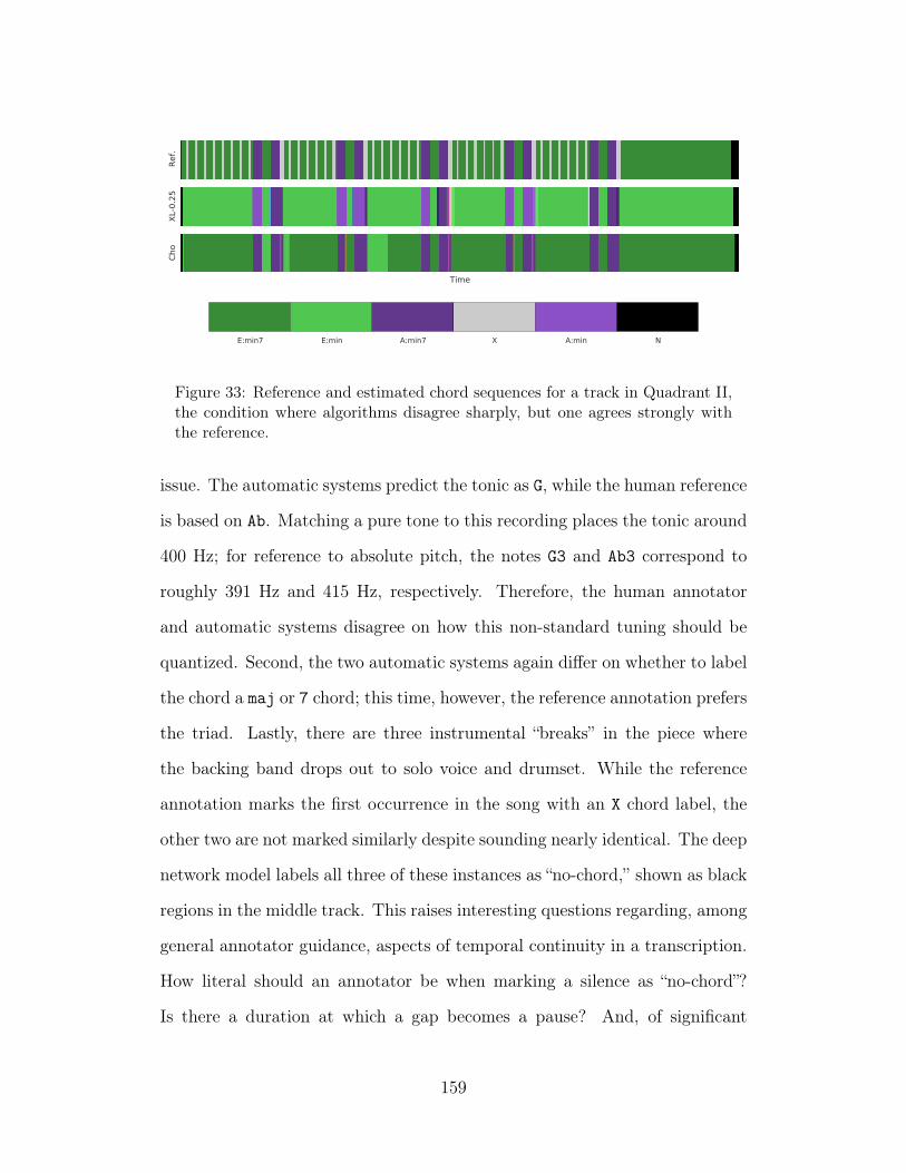
Ref.
XL-
0.2
5
Time
Cho
E:min7 E:min A:min7 X A:min N
Figure 33: Reference and estimated chord sequences for a track in Quadrant II,the condition where algorithms disagree sharply, but one agrees strongly withthe reference.
issue. The automatic systems predict the tonic as G, while the human reference
is based on Ab. Matching a pure tone to this recording places the tonic around
400 Hz; for reference to absolute pitch, the notes G3 and Ab3 correspond to
roughly 391 Hz and 415 Hz, respectively. Therefore, the human annotator
and automatic systems disagree on how this non-standard tuning should be
quantized. Second, the two automatic systems again differ on whether to label
the chord a maj or 7 chord; this time, however, the reference annotation prefers
the triad. Lastly, there are three instrumental “breaks” in the piece where
the backing band drops out to solo voice and drumset. While the reference
annotation marks the first occurrence in the song with an X chord label, the
other two are not marked similarly despite sounding nearly identical. The deep
network model labels all three of these instances as “no-chord,” shown as black
regions in the middle track. This raises interesting questions regarding, among
general annotator guidance, aspects of temporal continuity in a transcription.
How literal should an annotator be when marking a silence as “no-chord”?
Is there a duration at which a gap becomes a pause? And, of significant
159
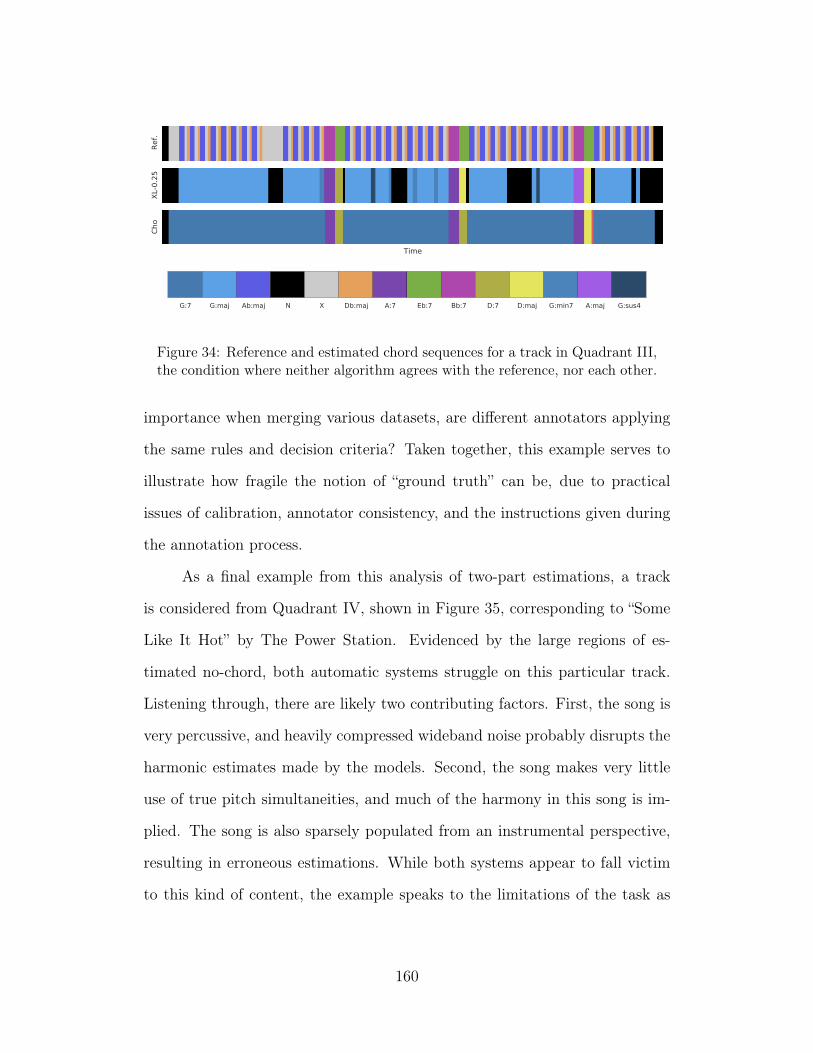
Ref.
XL-
0.2
5
Time
Cho
G:7 G:maj Ab:maj N X Db:maj A:7 Eb:7 Bb:7 D:7 D:maj G:min7 A:maj G:sus4
Figure 34: Reference and estimated chord sequences for a track in Quadrant III,the condition where neither algorithm agrees with the reference, nor each other.
importance when merging various datasets, are different annotators applying
the same rules and decision criteria? Taken together, this example serves to
illustrate how fragile the notion of “ground truth” can be, due to practical
issues of calibration, annotator consistency, and the instructions given during
the annotation process.
As a final example from this analysis of two-part estimations, a track
is considered from Quadrant IV, shown in Figure 35, corresponding to “Some
Like It Hot” by The Power Station. Evidenced by the large regions of es-
timated no-chord, both automatic systems struggle on this particular track.
Listening through, there are likely two contributing factors. First, the song is
very percussive, and heavily compressed wideband noise probably disrupts the
harmonic estimates made by the models. Second, the song makes very little
use of true pitch simultaneities, and much of the harmony in this song is im-
plied. The song is also sparsely populated from an instrumental perspective,
resulting in erroneous estimations. While both systems appear to fall victim
to this kind of content, the example speaks to the limitations of the task as
160
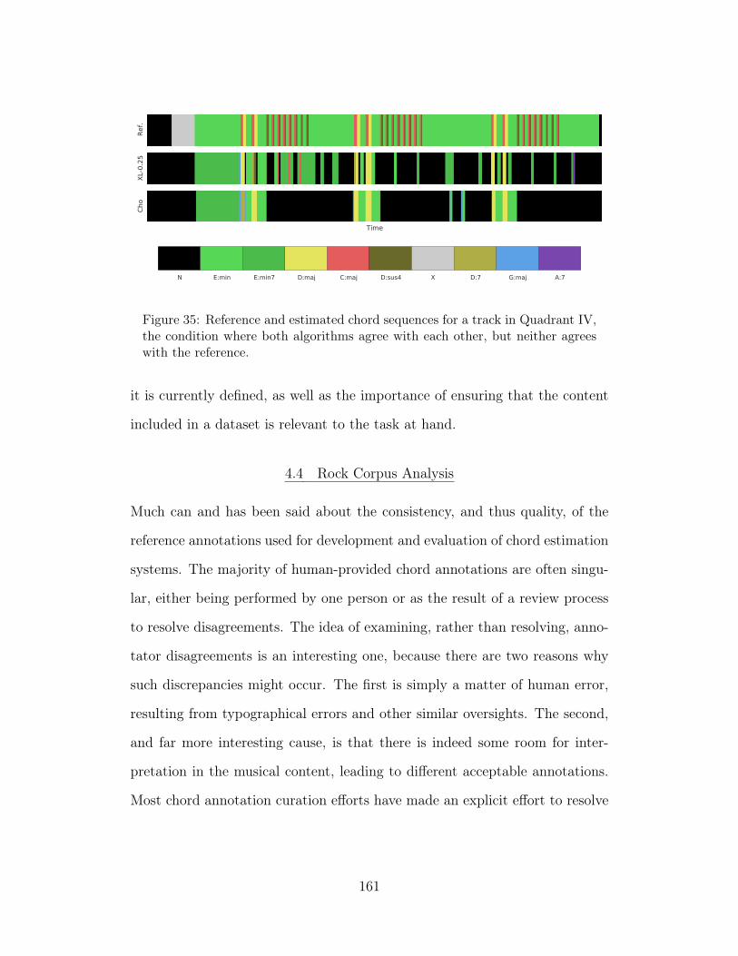
Ref.
XL-
0.2
5
Time
Cho
N E:min E:min7 D:maj C:maj D:sus4 X D:7 G:maj A:7
Figure 35: Reference and estimated chord sequences for a track in Quadrant IV,the condition where both algorithms agree with each other, but neither agreeswith the reference.
it is currently defined, as well as the importance of ensuring that the content
included in a dataset is relevant to the task at hand.
4.4 Rock Corpus Analysis
Much can and has been said about the consistency, and thus quality, of the
reference annotations used for development and evaluation of chord estimation
systems. The majority of human-provided chord annotations are often singu-
lar, either being performed by one person or as the result of a review process
to resolve disagreements. The idea of examining, rather than resolving, anno-
tator disagreements is an interesting one, because there are two reasons why
such discrepancies might occur. The first is simply a matter of human error,
resulting from typographical errors and other similar oversights. The second,
and far more interesting cause, is that there is indeed some room for inter-
pretation in the musical content, leading to different acceptable annotations.
Most chord annotation curation efforts have made an explicit effort to resolve
161
all discrepancies to a canonical transcription, however, and it is not possible
to explore any such instances in the data used so far.
Fortunately, the Rock Corpus dataset, first introduced in (De Clercq
& Temperley, 2011), is a set of 200 popular rock tracks with time-aligned
chord and melody transcriptions performed by two expert musicians: one, a
pianist, and the other, a guitarist. This insight into musical expertise adds an
interesting dimension to the inquiry when attempting to understand alternate
interpretations by the annotators. This collection of chord transcriptions has
seen little use in the ACE literature, as its initial release lacked timing data
for the transcriptions, and the chord names are provided in a Roman Numeral
syntax. A subsequent release fixed the former issue, however, in addition
to doubling the size of the collection. The latter issue is more a matter of
convenience, as key information is provided with the transcriptions and this
format can be translated to absolute chord names, consistent with the syntax
in Section 1.3. This dataset provides a previously uncapitalized opportunity
to explore the behavior of ACE systems as a function of multiple reference
transcriptions.
As an initial step, the two annotators, referred to here as DT and TdC,
are each used as a reference and estimation perspective in order to quantify the
agreement between them. The results, given in Table 21, indicate a high, but
imperfect level of consistency between the two human perspectives. Following
earlier trends, this is also a function of the chord spelling complexity, whereby
equivalence at the “root” is much higher than for “tetrads”. Additionally, it
is worth noting the asymmetry in chord comparisons. Thus, depending on
the perspective used as the reference, a estimation may match better or worse
with it. Finally, it is curious that the “MIREX” score is not perfect, a measure
162
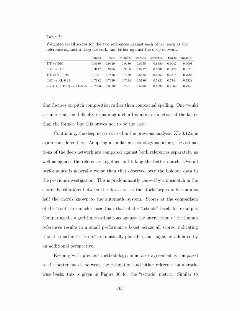
Table 21
Weighted recall scores for the two references against each other, each as thereference against a deep network, and either against the deep network.
triads root MIREX tetrads sevenths thirds majmin
DT vs TdC 0.8986 0.9329 0.9180 0.8355 0.8380 0.9042 0.9008
TdC vs DT 0.9117 0.9465 0.9168 0.8477 0.8537 0.9174 0.9176
DT vs XL-0.25 0.7051 0.7816 0.7180 0.5625 0.5653 0.7314 0.7084
TdC vs XL-0.25 0.7182 0.7939 0.7314 0.5786 0.5822 0.7444 0.7228
max(DT | TdC) vs XL-0.25 0.7306 0.8010 0.7431 0.5998 0.6032 0.7569 0.7348
that focuses on pitch composition rather than contextual spelling. One would
assume that the difficulty in naming a chord is more a function of the latter
than the former, but this proves not to be the case.
Continuing, the deep network used in the previous analysis, XL-0.125, is
again considered here. Adopting a similar methodology as before, the estima-
tions of the deep network are compared against both references separately, as
well as against the references together and taking the better match. Overall
performance is generally worse than that observed over the holdout data in
the previous investigation. This is predominantly caused by a mismatch in the
chord distributions between the datasets, as the RockCorpus only contains
half the chords known to the automatic system. Scores at the comparison
of the “root” are much closer than that of the “tetrads” level, for example.
Comparing the algorithmic estimations against the intersection of the human
references results in a small performance boost across all scores, indicating
that the machine’s “errors” are musically plausible, and might be validated by
an additional perspective.
Keeping with previous methodology, annotator agreement is compared
to the better match between the estimation and either reference on a track-
wise basis; this is given in Figure 36 for the “tetrads” metric. Similar to
163
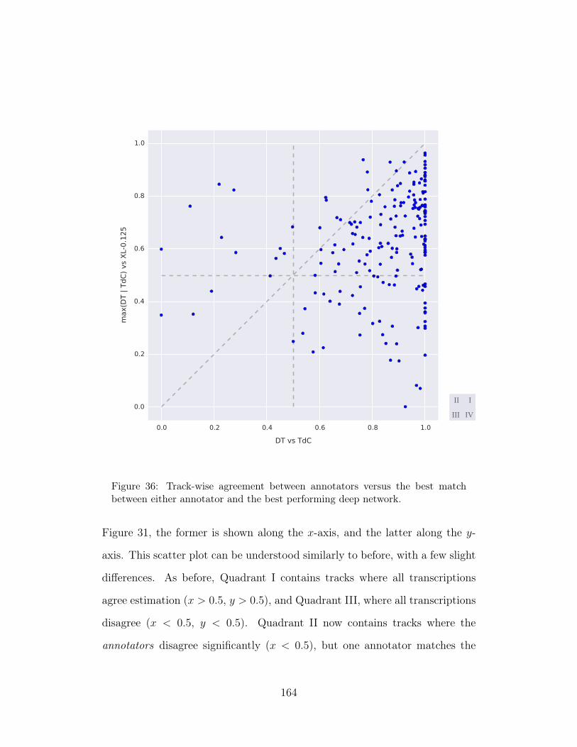
III
I
III IV
Figure 36: Track-wise agreement between annotators versus the best matchbetween either annotator and the best performing deep network.
Figure 31, the former is shown along the x-axis, and the latter along the y-
axis. This scatter plot can be understood similarly to before, with a few slight
differences. As before, Quadrant I contains tracks where all transcriptions
agree estimation (x > 0.5, y > 0.5), and Quadrant III, where all transcriptions
disagree (x < 0.5, y < 0.5). Quadrant II now contains tracks where the
annotators disagree significantly (x < 0.5), but one annotator matches the
164
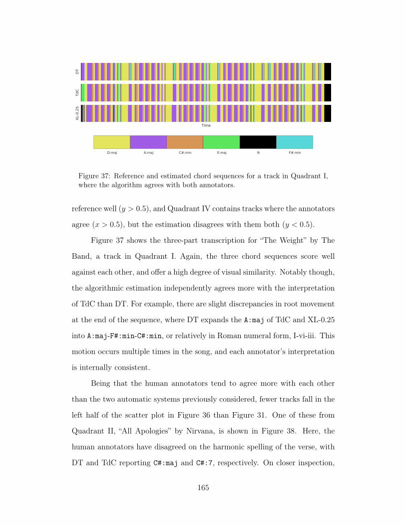
DT
TdC
Time
XL-
0.2
5
D:maj A:maj C#:min E:maj N F#:min
Figure 37: Reference and estimated chord sequences for a track in Quadrant I,where the algorithm agrees with both annotators.
reference well (y > 0.5), and Quadrant IV contains tracks where the annotators
agree (x > 0.5), but the estimation disagrees with them both (y < 0.5).
Figure 37 shows the three-part transcription for “The Weight” by The
Band, a track in Quadrant I. Again, the three chord sequences score well
against each other, and offer a high degree of visual similarity. Notably though,
the algorithmic estimation independently agrees more with the interpretation
of TdC than DT. For example, there are slight discrepancies in root movement
at the end of the sequence, where DT expands the A:maj of TdC and XL-0.25
into A:maj-F#:min-C#:min, or relatively in Roman numeral form, I-vi-iii. This
motion occurs multiple times in the song, and each annotator’s interpretation
is internally consistent.
Being that the human annotators tend to agree more with each other
than the two automatic systems previously considered, fewer tracks fall in the
left half of the scatter plot in Figure 36 than Figure 31. One of these from
Quadrant II, “All Apologies” by Nirvana, is shown in Figure 38. Here, the
human annotators have disagreed on the harmonic spelling of the verse, with
DT and TdC reporting C#:maj and C#:7, respectively. On closer inspection,
165
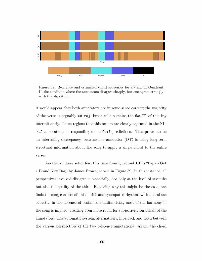
DT
TdC
Time
XL-
0.2
5
C#:maj C#:7 F#:maj Ab:maj N
Figure 38: Reference and estimated chord sequences for a track in QuadrantII, the condition where the annotators disagree sharply, but one agrees stronglywith the algorithm.
it would appear that both annotators are in some sense correct; the majority
of the verse is arguably C#:maj, but a cello sustains the flat-7th of this key
intermittently. These regions that this occurs are clearly captured in the XL-
0.25 annotation, corresponding to its C#:7 predictions. This proves to be
an interesting discrepancy, because one annotator (DT) is using long-term
structural information about the song to apply a single chord to the entire
verse.
Another of these select few, this time from Quadrant III, is “Papa’s Got
a Brand New Bag” by James Brown, shown in Figure 39. In this instance, all
perspectives involved disagree substantially, not only at the level of sevenths
but also the quality of the third. Exploring why this might be the case, one
finds the song consists of unison riffs and syncopated rhythms with liberal use
of rests. In the absence of sustained simultaneities, most of the harmony in
the song is implied, creating even more room for subjectivity on behalf of the
annotators. The automatic system, alternatively, flips back and forth between
the various perspectives of the two reference annotations. Again, the chord
166
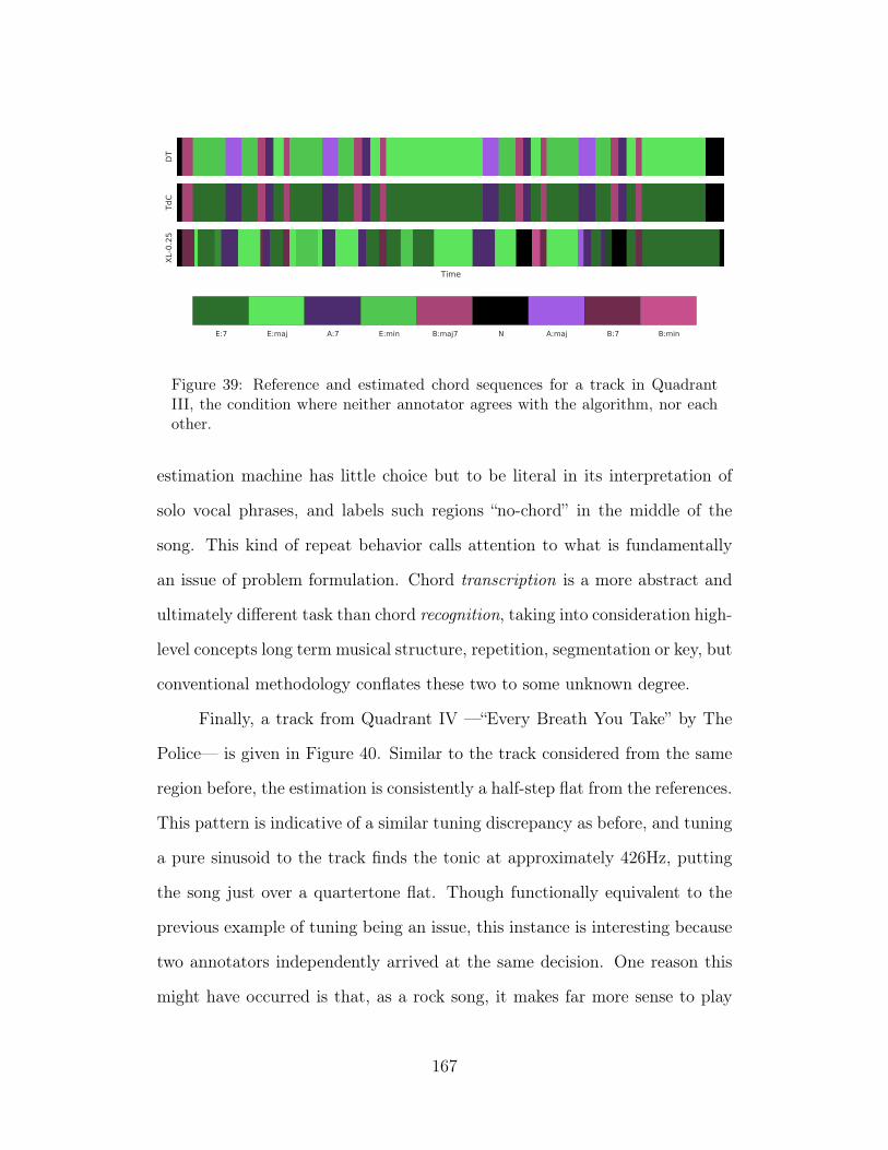
DT
TdC
Time
XL-
0.2
5
E:7 E:maj A:7 E:min B:maj7 N A:maj B:7 B:min
Figure 39: Reference and estimated chord sequences for a track in QuadrantIII, the condition where neither annotator agrees with the algorithm, nor eachother.
estimation machine has little choice but to be literal in its interpretation of
solo vocal phrases, and labels such regions “no-chord” in the middle of the
song. This kind of repeat behavior calls attention to what is fundamentally
an issue of problem formulation. Chord transcription is a more abstract and
ultimately different task than chord recognition, taking into consideration high-
level concepts long term musical structure, repetition, segmentation or key, but
conventional methodology conflates these two to some unknown degree.
Finally, a track from Quadrant IV —“Every Breath You Take” by The
Police— is given in Figure 40. Similar to the track considered from the same
region before, the estimation is consistently a half-step flat from the references.
This pattern is indicative of a similar tuning discrepancy as before, and tuning
a pure sinusoid to the track finds the tonic at approximately 426Hz, putting
the song just over a quartertone flat. Though functionally equivalent to the
previous example of tuning being an issue, this instance is interesting because
two annotators independently arrived at the same decision. One reason this
might have occurred is that, as a rock song, it makes far more sense to play
167
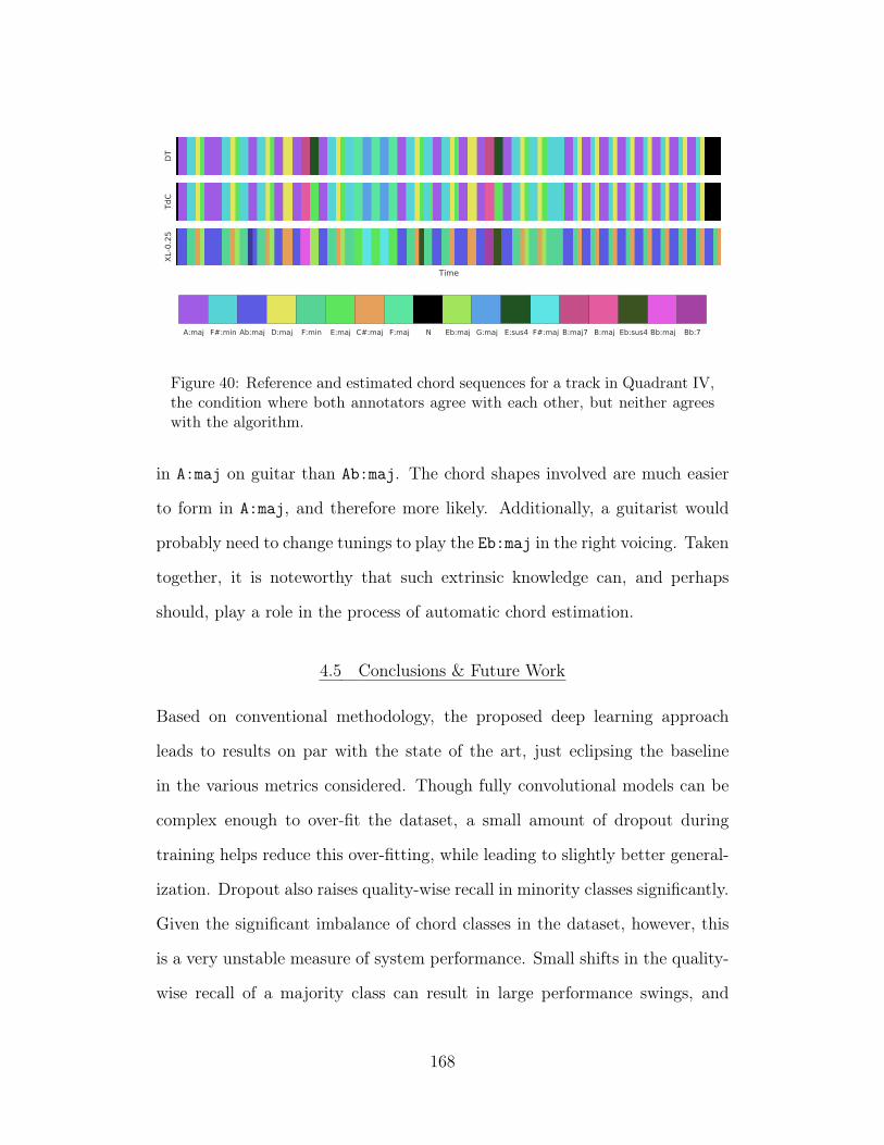
DT
TdC
Time
XL-
0.2
5
A:maj F#:min Ab:maj D:maj F:min E:maj C#:maj F:maj N Eb:maj G:maj E:sus4 F#:maj B:maj7 B:maj Eb:sus4 Bb:maj Bb:7
Figure 40: Reference and estimated chord sequences for a track in Quadrant IV,the condition where both annotators agree with each other, but neither agreeswith the algorithm.
in A:maj on guitar than Ab:maj. The chord shapes involved are much easier
to form in A:maj, and therefore more likely. Additionally, a guitarist would
probably need to change tunings to play the Eb:maj in the right voicing. Taken
together, it is noteworthy that such extrinsic knowledge can, and perhaps
should, play a role in the process of automatic chord estimation.
4.5 Conclusions & Future Work
Based on conventional methodology, the proposed deep learning approach
leads to results on par with the state of the art, just eclipsing the baseline
in the various metrics considered. Though fully convolutional models can be
complex enough to over-fit the dataset, a small amount of dropout during
training helps reduce this over-fitting, while leading to slightly better general-
ization. Dropout also raises quality-wise recall in minority classes significantly.
Given the significant imbalance of chord classes in the dataset, however, this
is a very unstable measure of system performance. Small shifts in the quality-
wise recall of a majority class can result in large performance swings, and
168
vice versa. Thus, the criteria for what makes for a “good” system may be
motivated by use case, to determine which of these metrics correspond to the
desired behavior.
Additionally, the suite of chord comparison functions demonstrate that
most errors between reference and estimation are hierarchical, and increase
with specificity of the chord, e.g. from root to triads to tetrads. One-of-
K classifiers struggle to encode these relationships between certain chords,
e.g. A:maj and A:maj7. By analogy, this is like building a classifier that
discriminates between, among other classes, animals and cats, respectively;
all cats are animals, but not all animals are cats. This is problematic in a
flat classifier, because it is attempting to linearly separate a pocket of density
contained within another. To address this issue, a structured output and
loss function would be better suited to model these relationships. Directly
encoding the knowledge that maj7 chords are a subset of maj, will make it
easier for a machine to learn these boundaries. One such hierarchy for the
chords considered in this work is given in Figure 41. Here, the degree of
specificity increases as the decision tree is traversed to a leaf node, and could
be achieved with more structured output, such as a hierarchical softmax or
conditional estimator.
In comparing the estimations of the two computational systems, deeper
insight is gained into the ground truth data used for development, and the
kinds of behavior, both the good and bad, that such approaches are prone
to exhibit. First, it is observed that they make rather different predictions
and their responses could be combined, motivating the exploration of ensem-
ble methods. Looking at performance at the track-level, alternatively, helps
identify problematic or noisy data in a collection. This is similar in spirit
169
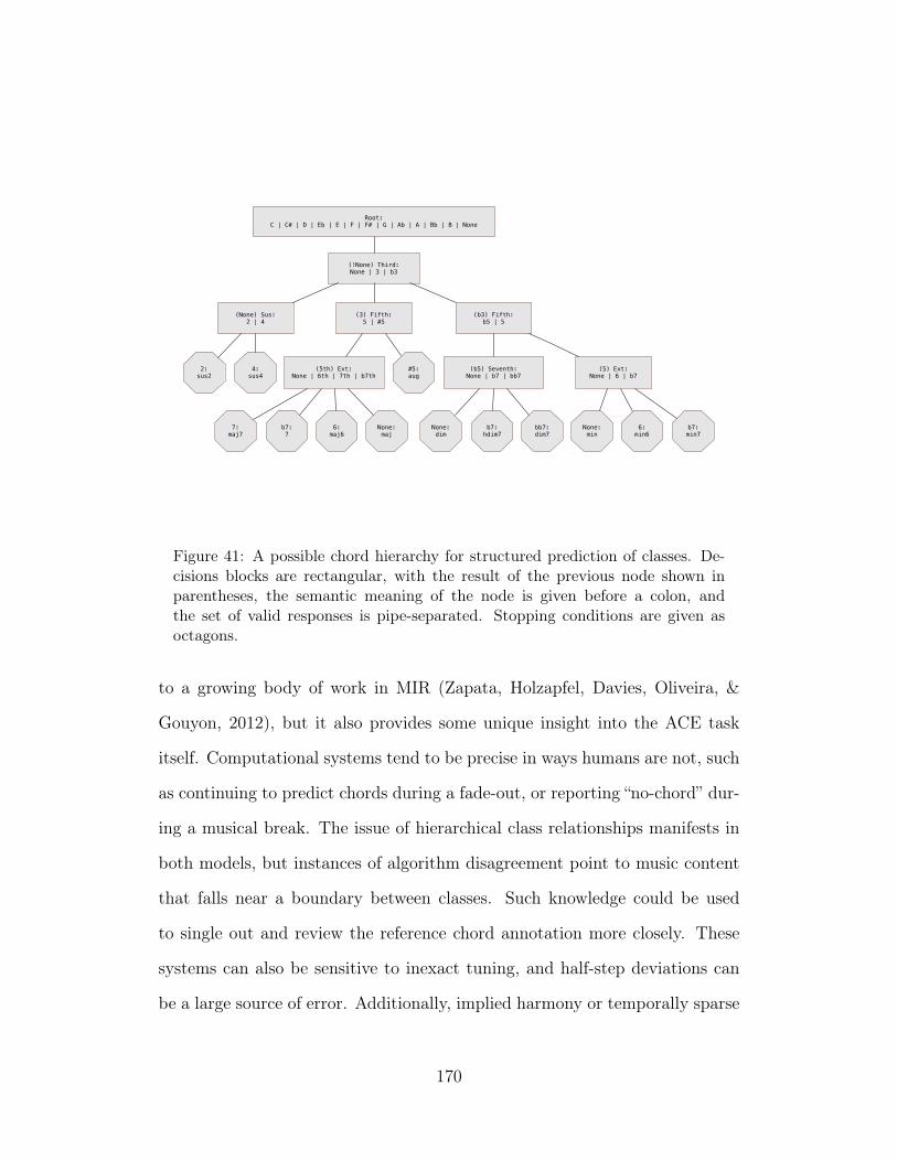
(!None) Third:None | 3 | b3
(5th) Ext: None | 6th | 7th | b7th
7:maj7
(b5) Seventh: None | b7 | bb7
b7:7
None:dim
(None) Sus:2 | 4
2:sus2
6:maj6
4:sus4
(3) Fifth:5 | #5
None:maj
#5:aug
(b3) Fifth:b5 | 5
b7:hdim7
bb7:dim7
(5) Ext:None | 6 | b7
None:min
6:min6
b7:min7
Root:C | C# | D | Eb | E | F | F# | G | Ab | A | Bb | B | None
Figure 41: A possible chord hierarchy for structured prediction of classes. De-cisions blocks are rectangular, with the result of the previous node shown inparentheses, the semantic meaning of the node is given before a colon, andthe set of valid responses is pipe-separated. Stopping conditions are given asoctagons.
to a growing body of work in MIR (Zapata, Holzapfel, Davies, Oliveira, &
Gouyon, 2012), but it also provides some unique insight into the ACE task
itself. Computational systems tend to be precise in ways humans are not, such
as continuing to predict chords during a fade-out, or reporting “no-chord” dur-
ing a musical break. The issue of hierarchical class relationships manifests in
both models, but instances of algorithm disagreement point to music content
that falls near a boundary between classes. Such knowledge could be used
to single out and review the reference chord annotation more closely. These
systems can also be sensitive to inexact tuning, and half-step deviations can
be a large source of error. Additionally, implied harmony or temporally sparse
170
patterns can be especially problematic, resulting in an over-estimation of the
“no-chord” class.
Conversely, leveraging multiple annotations for a given track provides a
deeper understanding of the errors a computational system might make. As
seen here, the assessment of a system will change depending on which in-
terpretation is taken as a reference, and a computational system may agree
with another human’s perspective, consistent with the work of McVicar (Ni,
McVicar, Santos-Rodriguez, & De Bie, 2013). Most important is the recog-
nition that human annotators do not agree all the time, and that describing
some music content in the language of chords is inherently subjective. In such
cases, there is no “ground truth” to speak of, and multiple chord labels may be
acceptable. This is a critical observation, and one that cuts strongly against
the long-standing methodology of curating ground truth references in ACE.
Stated previously, the sole purpose of an objective measure is that it serves as
a reasonable proxy for subjective experience. If the goal of ACE is to produce
a chord annotation on par with that of a qualified human —a musical Turing
test of sorts— then the reference annotation at hand may be only one of many
valid perspectives. As a result, evaluating against a singular perspective is
leading to results that may be inconsistent with subjective experience.
Instead, embracing multiple perspectives, rather than attempting to re-
solve them into a canonical target, would allow for more stable evaluation of
computational models. One such way this could be achieved is by obtaining
multiple chord annotations and creating a time-aligned bag of words reference.
For example, knowing that 97 of 100 annotators labeled a chord as A:7 is very
different from the scenario that 52 did, while the other 48 reported A:maj.
Curating a dataset with so many perspectives is unlikely to happen, but per-
171
haps multiple computational systems could be used to find boundary chords
that do warrant multiple perspectives. Ultimately, this study demonstrates
that future chord datasets should strive to capture the degree of subjectivity
in an annotation, thus enabling objective measures better correspond with
subjective experience.
5 Summary
In this chapter, the application of deep learning to ACE has been thoroughly
explored. By standard evaluation practices, competitive performance is demon-
strated on both a major-minor and large-vocabulary formulation of the task.
Importantly, much effort is invested in understanding both the behavior of
the computational systems discussed, as well as the reference data used to
evaluate performance. Perhaps the most important finding is that the current
state of the art may have truly hit a glass ceiling, due to the conventional
practice of building and testing against “ground truth” datasets for an all too
often subjective task. This challenge is further compounded by approaches to
prediction and evaluation, which attempt to perform flat classification of a hi-
erarchically structured chord taxonomy. Thus, while there is almost certainly
room for improvement, the exploration here indicates that the vast majority
of error in modern chord recognition systems is a result of invalid assumptions
baked into the very task.
Notably, four issues with current chord estimation methodology have
been identified in this work. One, it seems necessary that computational mod-
els embrace structured outputs; one-of-K class encoding schemes introduce
unnecessary complexity between what are naturally hierarchical relationships.
172
Two, the community fundamentally needs to better distinguish between the
two tasks at hand, being chord recognition —I am playing this literal chord
on guitar— and chord transcription —finding the best chord label to describe
this harmonically homogeneous region of music— and how this is articulated
to reference annotation authors. Three, chord transcription requires more ex-
plicit segmentation, rather than letting such boundaries between regions of
harmonic stability result implicitly from post-filtering algorithms. Lastly, the
often subjective nature of chord labeling needs to be acknowledged in the
process of curating reference data, and the human labeling task should com-
bine multiple perspectives rather than attempt to yield a canonical “expert”
reference.
173
CHAPTER VI
FROM MUSIC AUDIO TO GUITAR TABLATURE
In the previous chapter, it was demonstrated that state of the art ACE
systems perform at a relatively high level, often producing reasonable, if not
exact, chord estimations. Deploying these systems in the wild for real users,
however, presents two practical difficulties: one, performing a given chord
sequence requires that the musician knows how to play each chord on their
instrument of choice; and two, the performance of classification-minded chord
estimation systems does not degrade gracefully, especially for those lacking
a good music theory background. Recognizing that guitarists account for a
large majority of the music community, both challenges are addressed here
by designing a deep convolutional network to model the physical constraints
of a guitar’s fretboard, directly producing human-readable representations of
music audio, i.e. tablature.
Approaching chord estimation through the lens of guitar tablature offers
a variety of critical benefits. Guitar chord shapes impose an explicit hierarchy
among notes in a chord family, such that related chords are forced to be
near-neighbors in the output space. This constrains the learning problem in
musically meaningful ways, and enables the model to produce outputs beyond
the lexicon of chords used for training. The human-readable nature of the
system’s output is also valuable from a user perspective, being immediately
useful with minimal prerequisite knowledge. Furthermore, a softer prediction
174
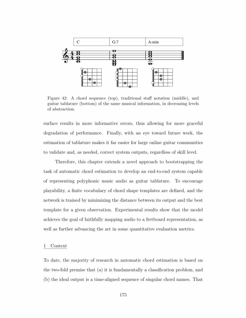
C G:7 A:min
Figure 42: A chord sequence (top), traditional staff notation (middle), andguitar tablature (bottom) of the same musical information, in decreasing levelsof abstraction.
surface results in more informative errors, thus allowing for more graceful
degradation of performance. Finally, with an eye toward future work, the
estimation of tablature makes it far easier for large online guitar communities
to validate and, as needed, correct system outputs, regardless of skill level.
Therefore, this chapter extends a novel approach to bootstrapping the
task of automatic chord estimation to develop an end-to-end system capable
of representing polyphonic music audio as guitar tablature. To encourage
playability, a finite vocabulary of chord shape templates are defined, and the
network is trained by minimizing the distance between its output and the best
template for a given observation. Experimental results show that the model
achieves the goal of faithfully mapping audio to a fretboard representation, as
well as further advancing the art in some quantitative evaluation metrics.
1 Context
To date, the majority of research in automatic chord estimation is based on
the two-fold premise that (a) it is fundamentally a classification problem, and
(b) the ideal output is a time-aligned sequence of singular chord names. That
175
said, it is worthwhile to reconsider how the development of such systems is
motivated by the goal of helping the ambitious musician learn to play a par-
ticular song. Notably, today guitarists comprise one of the largest groups of
musicians attempting to do just that. Over the last century, the guitar, in all
of its forms, has drastically risen in popularity and prevalence, both in profes-
sional and amateur settings. Given the low start-up cost, portability, favorable
learning curve, and —courtesy of musicians like Jimi Hendrix or The Beatles—
an undisputed “cool factor” in Western popular culture, it is unsurprising that
guitars dwarf music instrument sales in the United States. Based on the 2014
annual report of the National Association of Music Merchants (NAMM), a
whopping 2.47M guitars were sold in 2013 in the United States, accounting
for a retail value of $1.07 billion USD (of Music Merchants, 2014); as a point
of comparison, all wind instruments combined —the next largest instrument
category— totaled just over half that figure, at $521M USD.
The fact that guitarists comprise such a large portion of the musician
community is important, as it affects how they might prefer to interact with
a chord estimation system. While most instruments make use of traditional
staff notation, fretted instruments, like lute or guitar, have a long history of
using tablature to notate music. Illustrated in Figure 42, tablature requires
minimal musical knowledge to interpret, and thus offers the advantage that
is easier to read, particularly for beginners. Whereas staff notation explicitly
encodes pitch information, leaving the performer to translate notes to a given
instrument, tablature explicitly encodes performance instructions for a given
instrument. Though it can be difficult to accurately depict rhythmic informa-
tion with tablature, this is seldom an obstacle for guitarists. Chords-centric
176
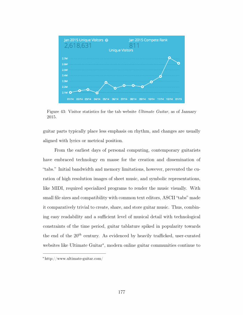
Figure 43: Visitor statistics for the tab website Ultimate Guitar, as of January2015.
guitar parts typically place less emphasis on rhythm, and changes are usually
aligned with lyrics or metrical position.
From the earliest days of personal computing, contemporary guitarists
have embraced technology en masse for the creation and dissemination of
“tabs.” Initial bandwidth and memory limitations, however, prevented the cu-
ration of high resolution images of sheet music, and symbolic representations,
like MIDI, required specialized programs to render the music visually. With
small file sizes and compatibility with common text editors, ASCII “tabs” made
it comparatively trivial to create, share, and store guitar music. Thus, combin-
ing easy readability and a sufficient level of musical detail with technological
constraints of the time period, guitar tablature spiked in popularity towards
the end of the 20th century. As evidenced by heavily trafficked, user-curated
websites like Ultimate Guitar∗, modern online guitar communities continue to
∗http://www.ultimate-guitar.com/
177
place a high demand on tablature. Shown in Figure 43, this website alone
sees, on average, over 2M unique visitors∗ per month in the United States.
Taken together, these observations motivate an obvious conclusion. Gui-
tarists comprise a significant portion of the global music community, and are
actively creating and using tablature as a means of learning music. An au-
tomatic chord estimation system would be extremely valuable to this demo-
graphic, but such a system should be sensitive to the common preference for
tablature. Therefore, this chapter is an effort to steer automatic chord esti-
mation toward a specific application, in order to address a potential use case
for a very real demographic.
2 Proposed System
Building on previous efforts in automatic chord estimation, the best perform-
ing configuration presented in Chapter 5, XL-0.125, is extended here for guitar
chord estimation. As such, many design decisions remain consistent with the
previous description, such as the constant-Q representation, dataset, or eval-
uation methodology, and are omitted from the discussion. There are a few
important differences, however, which are addressed below. First, the archi-
tecture is modified slightly to produce fretboard-like outputs. A strategy is
then discussed for incorporating guitar chord shapes into the model. The
modified objective and decision functions are presented last, detailing how the
model is optimized and use to estimate discrete chord classes.
Finally, it is worth mentioning that, despite the desire to map notes to a
guitar fretboard, this approach is much closer in principle to chord estimation
∗Based on Compete.com analytics data, accessed on 15 March, 2015.
178
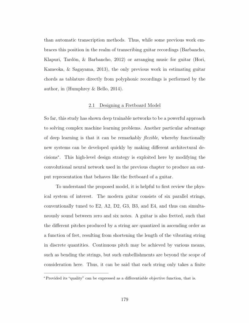
than automatic transcription methods. Thus, while some previous work em-
braces this position in the realm of transcribing guitar recordings (Barbancho,
Klapuri, Tardón, & Barbancho, 2012) or arranging music for guitar (Hori,
Kameoka, & Sagayama, 2013), the only previous work in estimating guitar
chords as tablature directly from polyphonic recordings is performed by the
author, in (Humphrey & Bello, 2014).
2.1 Designing a Fretboard Model
So far, this study has shown deep trainable networks to be a powerful approach
to solving complex machine learning problems. Another particular advantage
of deep learning is that it can be remarkably flexible, whereby functionally
new systems can be developed quickly by making different architectural de-
cisions∗. This high-level design strategy is exploited here by modifying the
convolutional neural network used in the previous chapter to produce an out-
put representation that behaves like the fretboard of a guitar.
To understand the proposed model, it is helpful to first review the phys-
ical system of interest. The modern guitar consists of six parallel strings,
conventionally tuned to E2, A2, D2, G3, B3, and E4, and thus can simulta-
neously sound between zero and six notes. A guitar is also fretted, such that
the different pitches produced by a string are quantized in ascending order as
a function of fret, resulting from shortening the length of the vibrating string
in discrete quantities. Continuous pitch may be achieved by various means,
such as bending the strings, but such embellishments are beyond the scope of
consideration here. Thus, it can be said that each string only takes a finite
∗Provided its “quality” can be expressed as a differentiable objective function, that is.
179
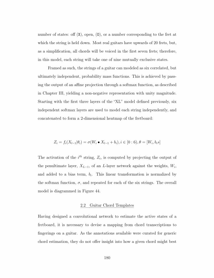
number of states: off (X), open, (O), or a number corresponding to the fret at
which the string is held down. Most real guitars have upwards of 20 frets, but,
as a simplification, all chords will be voiced in the first seven frets; therefore,
in this model, each string will take one of nine mutually exclusive states.
Framed as such, the strings of a guitar can modeled as six correlated, but
ultimately independent, probability mass functions. This is achieved by pass-
ing the output of an affine projection through a softmax function, as described
in Chapter III, yielding a non-negative representation with unity magnitude.
Starting with the first three layers of the “XL” model defined previously, six
independent softmax layers are used to model each string independently, and
concatenated to form a 2-dimensional heatmap of the fretboard:
Zi = fi(Xl−1|θi) = σ(Wi •Xl−1 + bi), i ∈ [0 : 6), θ = [Wi, bis]
The activation of the ith string, Zi, is computed by projecting the output of
the penultimate layer, XL−1, of an L-layer network against the weights, Wi,
and added to a bias term, bi. This linear transformation is normalized by
the softmax function, σ, and repeated for each of the six strings. The overall
model is diagrammed in Figure 44.
2.2 Guitar Chord Templates
Having designed a convolutional network to estimate the active states of a
fretboard, it is necessary to devise a mapping from chord transcriptions to
fingerings on a guitar. As the annotations available were curated for generic
chord estimation, they do not offer insight into how a given chord might best
180
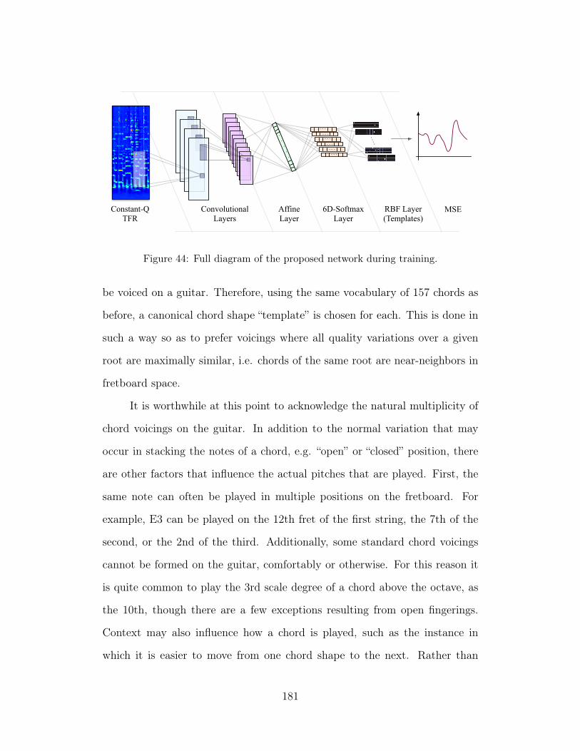
ConvolutionalLayers
AffineLayer
6D-SoftmaxLayer
RBF Layer(Templates)
MSEConstant-QTFR
Figure 44: Full diagram of the proposed network during training.
be voiced on a guitar. Therefore, using the same vocabulary of 157 chords as
before, a canonical chord shape “template” is chosen for each. This is done in
such a way so as to prefer voicings where all quality variations over a given
root are maximally similar, i.e. chords of the same root are near-neighbors in
fretboard space.
It is worthwhile at this point to acknowledge the natural multiplicity of
chord voicings on the guitar. In addition to the normal variation that may
occur in stacking the notes of a chord, e.g. “open” or “closed” position, there
are other factors that influence the actual pitches that are played. First, the
same note can often be played in multiple positions on the fretboard. For
example, E3 can be played on the 12th fret of the first string, the 7th of the
second, or the 2nd of the third. Additionally, some standard chord voicings
cannot be formed on the guitar, comfortably or otherwise. For this reason it
is quite common to play the 3rd scale degree of a chord above the octave, as
the 10th, though there are a few exceptions resulting from open fingerings.
Context may also influence how a chord is played, such as the instance in
which it is easier to move from one chord shape to the next. Rather than
181
attempt to address all of these issues now, the canonical template approach is
chosen as a practical means to simplify overall system design. The choice of
one template over another likely has nontrivial implications for the behavior
of the model, but this is left as a variable to be explored in the future.
2.3 Decision Functions
While estimating frets is sufficient for human interpretation, it is necessary to
design two related decision functions in order to allow the machine to operate
automatically. First, the templates defined above must be incorporated into an
objective function, such that the machine can learn to optimize this measure
over the training data. Finding inspiration in (LeCun et al., 1998), a Radial
Basis Function (RBF) layer is added to the network, given as follows:
E(Z|WT ) =∑
(Zout −WT [k])2 (28)
where Z is the output of the fretboard model, WT is a tensor of chord shape
templates with shape (K, 6, 9), such that K is the number of chord templates,
and k the index of the reference class. Note that these templates will impose
the proper organization on the output of the model, and thus remain fixed
during the learning process. Since these weights are constant, minimizing this
function does not require a contrastive penalty or margin term to prevent it
from collapsing, i.e. making all the squared distances zero.
Additionally, for the purposes of Viterbi post-filtering and fairly compar-
ing with previous results, the energy surface must be inverted into a likelihood
function. This is achieved by negating the energy function, E, and normalizing
as a Gibbs distribution:
182
L(Yk|X,Θ) =exp(−β E(Yk|X,Θ))∑Ki exp(−β E(Yk|X,Θ))
(29)
For the experiments detailed below, β = 1. It is conceivable that the
choice of hyperparameter may impact system behavior when coupled with the
Viterbi algorithm, but this value was empirically observed to give good results
and not explored further.
3 Experimental Method
The focus of this chapter now shifts toward the experimental method adopted
to investigate the behavior of this basic approach. Herein, the training strat-
egy, corresponding variables, and subsequent quantitative results are addressed
in turn.
3.1 Training Strategy
Though it is able to incorporate musical knowledge into the architectural de-
sign, the model proposed here is unable achieve root-invariant weight sharing
as in the previous chapter. This is due to root-dependent chord shapes result-
ing from the nonuniform arrangement of chords on the neck of the guitar. It
is important to consider the effect this has on system performance, as well as
other means of achieving “root invariance”, and thus three different training
strategies are employed here.
As a baseline condition, the model is trained with the natural distribu-
tion of the data (“as-is”). Note that it is reasonable to expect these models to
be deficient, as there may be chord class mismatch between training and test
conditions, i.e. chord classes in the test partition do not occur in the training
183
set. To address the imbalanced learning problem, the second training condi-
tion scales the loss of each training observation by a class-dependent weight
(“scaled”). These weights are determined by computing the root-invariant
prior over the training partition, taking its inverse, and standardizing the co-
efficients to unit mean and standard deviation. The third and final training
condition couples loss scaling with data augmentation, such that during train-
ing each datapoint is circularly shifted in frequency on the interval [−12, 12]
(“augmented”). This allows the variance of each chord quality to be evenly
distributed across classes, and helping prevent any missing class coverage in
the training set.
Identical partitions of the dataset used in the previous chapter are em-
ployed here; the dataset is split 68:12:20, into training, validation, and test,
respectively, and the partitions are rotated so that all data is used as a holdout
set once. All models are trained with mini-batch stochastic gradient descent
at a batch size of 100, learning rate of 0.02, and dropout ratio of 0.125. Train-
ing proceeded for several hundred iterations, ultimately bounded by a ceiling
of 24 hours, and parameters saved every 10k iterations. Model selection was
performed as a brute force search over both the parameter checkpoints and
self-transition penalty for Viterbi, from -20 to -40 in steps of 5. The best model
was chosen by the maximum of the harmonic mean of the chord evaluation
metrics outlined previously.
3.2 Quantitative Evaluation
In the absence of a thorough user study, the proposed approach is evaluated
against the chord estimation task posed in Chapter 5.4. Applying the method-
ology outlined above, the three training conditions were run to completion and
184
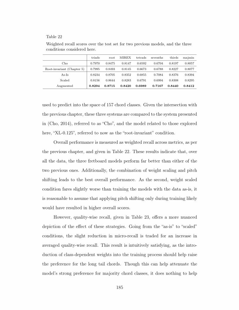
Table 22
Weighted recall scores over the test set for two previous models, and the threeconditions considered here.
triads root MIREX tetrads sevenths thirds majmin
Cho 0.7970 0.8475 0.8147 0.6592 0.6704 0.8197 0.8057
Root-invariant (Chapter 5) 0.7995 0.8493 0.8145 0.6673 0.6788 0.8227 0.8077
As-Is 0.8234 0.8705 0.8352 0.6855 0.7084 0.8376 0.8394
Scaled 0.8156 0.8644 0.8283 0.6791 0.6994 0.8308 0.8295
Augmented 0.8294 0.8715 0.8420 0.6989 0.7167 0.8440 0.8412
used to predict into the space of 157 chord classes. Given the intersection with
the previous chapter, these three systems are compared to the system presented
in (Cho, 2014), referred to as “Cho”, and the model related to those explored
here, “XL-0.125”, referred to now as the “root-invariant” condition.
Overall performance is measured as weighted recall across metrics, as per
the previous chapter, and given in Table 22. These results indicate that, over
all the data, the three fretboard models perform far better than either of the
two previous ones. Additionally, the combination of weight scaling and pitch
shifting leads to the best overall performance. As the second, weight scaled
condition fares slightly worse than training the models with the data as-is, it
is reasonable to assume that applying pitch shifting only during training likely
would have resulted in higher overall scores.
However, quality-wise recall, given in Table 23, offers a more nuanced
depiction of the effect of these strategies. Going from the “as-is” to “scaled”
conditions, the slight reduction in micro-recall is traded for an increase in
averaged quality-wise recall. This result is intuitively satisfying, as the intro-
duction of class-dependent weights into the training process should help raise
the preference for the long tail chords. Though this can help attenuate the
model’s strong preference for majority chord classes, it does nothing to help
185
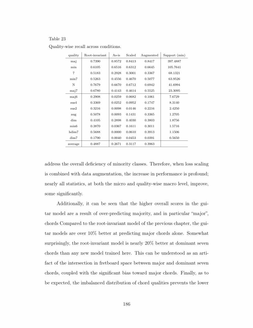
Table 23
Quality-wise recall across conditions.
quality Root-invariant As-is Scaled Augmented Support (min)
maj 0.7390 0.8572 0.8413 0.8417 397.4887
min 0.6105 0.6516 0.6312 0.6645 105.7641
7 0.5183 0.2928 0.3001 0.3367 68.1321
min7 0.5263 0.4556 0.4670 0.5077 63.9526
N 0.7679 0.6670 0.6712 0.6942 41.6994
maj7 0.6780 0.4143 0.4614 0.5525 23.3095
maj6 0.2908 0.0259 0.0682 0.1061 7.6729
sus4 0.3369 0.0252 0.0952 0.1747 8.3140
sus2 0.3216 0.0098 0.0146 0.2216 2.4250
aug 0.5078 0.0093 0.1431 0.3365 1.2705
dim 0.4105 0.2898 0.4030 0.3803 1.8756
min6 0.3870 0.0367 0.1611 0.3011 1.5716
hdim7 0.5688 0.0000 0.0610 0.3913 1.1506
dim7 0.1790 0.0040 0.0453 0.0391 0.5650
average 0.4887 0.2671 0.3117 0.3963
address the overall deficiency of minority classes. Therefore, when loss scaling
is combined with data augmentation, the increase in performance is profound;
nearly all statistics, at both the micro and quality-wise macro level, improve,
some significantly.
Additionally, it can be seen that the higher overall scores in the gui-
tar model are a result of over-predicting majority, and in particular “major”,
chords Compared to the root-invariant model of the previous chapter, the gui-
tar models are over 10% better at predicting major chords alone. Somewhat
surprisingly, the root-invariant model is nearly 20% better at dominant seven
chords than any new model trained here. This can be understood as an arti-
fact of the intersection in fretboard space between major and dominant seven
chords, coupled with the significant bias toward major chords. Finally, as to
be expected, the imbalanced distribution of chord qualities prevents the lower
186
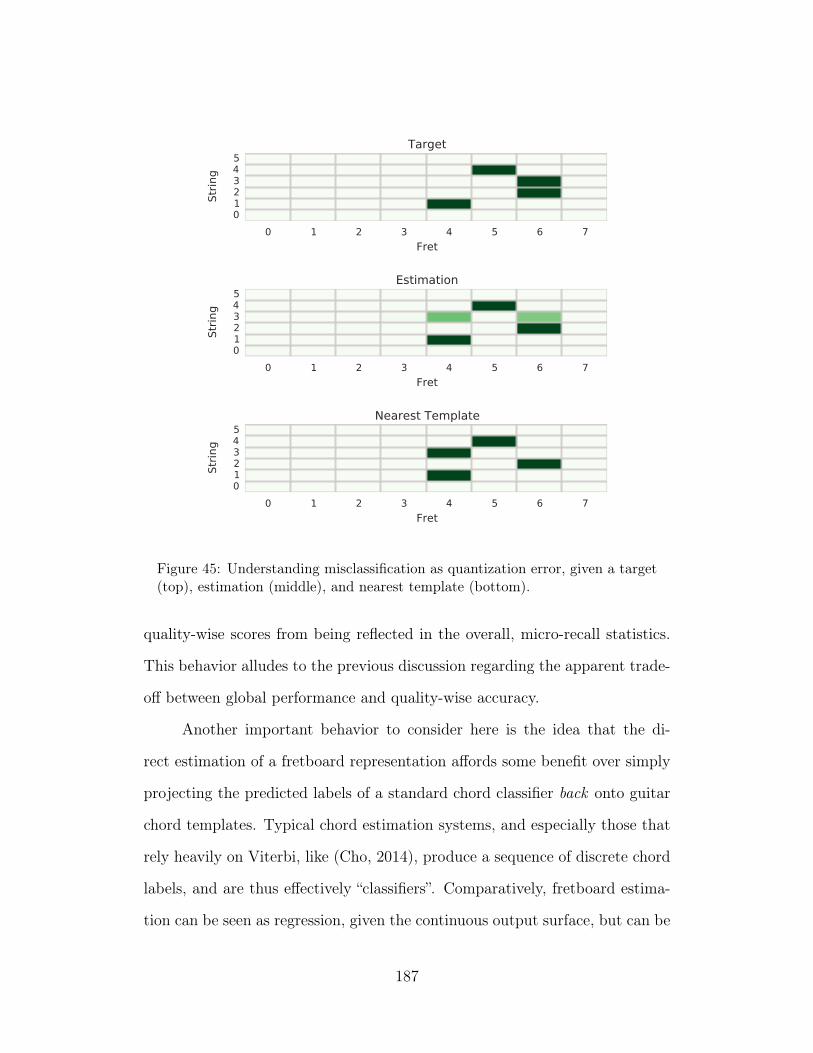
0 1 2 3 4 5 6 7
Fret
012345
Str
ing
Target
0 1 2 3 4 5 6 7
Fret
012345
Str
ing
Estimation
0 1 2 3 4 5 6 7
Fret
012345
Str
ing
Nearest Template
Figure 45: Understanding misclassification as quantization error, given a target(top), estimation (middle), and nearest template (bottom).
quality-wise scores from being reflected in the overall, micro-recall statistics.
This behavior alludes to the previous discussion regarding the apparent trade-
off between global performance and quality-wise accuracy.
Another important behavior to consider here is the idea that the di-
rect estimation of a fretboard representation affords some benefit over simply
projecting the predicted labels of a standard chord classifier back onto guitar
chord templates. Typical chord estimation systems, and especially those that
rely heavily on Viterbi, like (Cho, 2014), produce a sequence of discrete chord
labels, and are thus effectively “classifiers”. Comparatively, fretboard estima-
tion can be seen as regression, given the continuous output surface, but can be
187
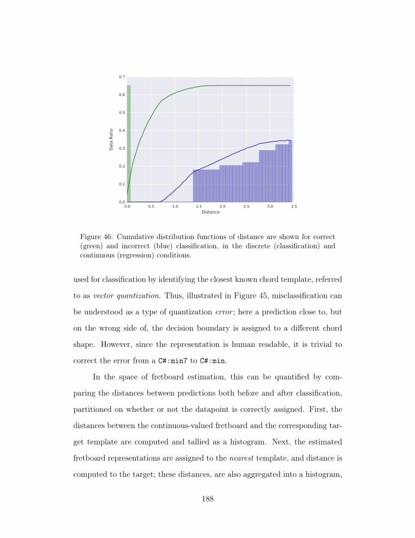
0.0 0.5 1.0 1.5 2.0 2.5 3.0 3.5
Distance
0.0
0.1
0.2
0.3
0.4
0.5
0.6
0.7
Data
Rati
o
Figure 46: Cumulative distribution functions of distance are shown for correct(green) and incorrect (blue) classification, in the discrete (classification) andcontinuous (regression) conditions.
used for classification by identifying the closest known chord template, referred
to as vector quantization. Thus, illustrated in Figure 45, misclassification can
be understood as a type of quantization error ; here a prediction close to, but
on the wrong side of, the decision boundary is assigned to a different chord
shape. However, since the representation is human readable, it is trivial to
correct the error from a C#:min7 to C#:min.
In the space of fretboard estimation, this can be quantified by com-
paring the distances between predictions both before and after classification,
partitioned on whether or not the datapoint is correctly assigned. First, the
distances between the continuous-valued fretboard and the corresponding tar-
get template are computed and tallied as a histogram. Next, the estimated
fretboard representations are assigned to the nearest template, and distance is
computed to the target; these distances, are also aggregated into a histogram,
188
but take only a finite number of values. Both probability density functions
are integrated into continuous distribution functions to illustrate what ratio
of the data lives within the radius of a bounding volume, shown in Figure 46.
Here, it can be seen that classification clearly widens the gap between correct
and incorrect answers. Alternatively, in the regression scenario, nearly 20% of
these errors are closer to their correct class, accounting for well over 80% of
the data. Importantly, the improved proximity of these errors mean that they
should be easier to correct by potential users.
4 Discussion
This chapter has proposed a method of extending a previous automatic chord
estimation by introducing the physical constraints of a guitar. Not only does
this yield a higher performing system, based on overall metrics, but the out-
puts are directly human readable making the system attractive from a user
experience standpoint. While the system seems to struggle more than pre-
vious efforts across all chord qualities, this is arguably an instance in which
performing better over all the data is preferable. The sample sizes of rare
chords in the dataset are at times too small to draw meaningful conclusions
about performance at the class level. Further complicating matters, there is
also some unknown degree of subjectivity in the reference annotations, used
for both training and evaluation. Pragmatically speaking though, consistently
tracking root motion, e.g. being in the right place on the neck, is probably
sufficient for most guitarists to deem such a system useful. The vast majority
of music can be simplified as “power chords”, consisting of the root and the
fifth, and often more detailed chords can be realized by modifying this basic
189
shape. Therefore, while many methodological challenges inherent to chord es-
timation persist in this study, predicting chord shapes as tablature softens the
degree to which they impact usability.
Setting aside the limitations of quantitative evaluation in chord estima-
tion, the proposed system warrants a subjective, user experience study in the
future. Many of the gains identified here can only be qualitatively assessing
how such a system achieves its goals, such as the degree to which performance
does in fact degrade gracefully. Countless instances can be identified where
system “errors” can be reasonably interpreted as the chord name provided, but
only a study with real users will indicate how useful this is.
Perhaps most importantly though, the next logical research step is to
develop an interactive user interface and deploy the system at scale. In addi-
tion to distributed instruction, deploying an “autotabbing” system provides a
means to collect and clean reference annotations. Approaching this task from
the perspective of human-readable representations holds considerable promise
in the space of data curation, as editing a chord transcription is generally a
far simpler task than creating one from scratch. This reality is only amplified
for annotators who lack formal ear training. Importantly though, this reduces
the prerequisite skill level, the amount of time needed to complete the task, or
both, required in the data authoring task. Therefore, this system creates the
potential to include a larger number of musicians across a wide array of skills
in the data collection process. More annotators not only opens the door for
more annotations, but multiple perspectives of the same music content. This
will be critical to the role subjectivity plays in chord estimation research, now
and in the near future.
190
CHAPTER VII
WORKFLOWS FOR REPRODUCIBLE RESEARCH
In recent years, the philosophy of open source software has begun taking
root in scientific research, particularly in the field of computer science. There
are several reasons why open research is beneficial to the greater body of hu-
man knowledge, but three are of particular value here. First, sharing code and
data allows others to reproduce previous results, a fundamental tenet of the
scientific method. Open source implementations are invaluable for sufficiently
complex systems. It may be near impossible to describe every minute detail
in a publication necessary for someone else to replicate the obtained results;
for some works, in fact, the only artifact that can do this unambiguously is
the source code itself. Second, and in a related vein, open research makes it
both easier and faster to build upon and extend the previous work of others.
Even in the instance a researcher is able to recreate a published system, the
time and effort necessary to get to this point is significant and arguably un-
necessary. Granted, while there is an educational component inherent to the
re-implementation of previous work, the situation is akin to long division: it
is certainly valuable to learn how to divide by hand, but no one shuns the
use of a calculator on a day to day basis. Lastly, it is a good and responsible
act to contribute tools and software back to the larger research community.
All research stands on the shoulders of previous efforts, from improving on a
recently published algorithm to the decades-old linear algebra routines doing
191
all its number crunching. The reality is that no one individual has ever truly
solved anything on their own, and sharing the fruits of one’s research endeavors
serves the common good.
With these motivations in mind, this chapter details the several open
source contributions made in the course of this work, culminating in a single
code repository used to produce the results contained herein. These software
tools consist of the following: Section 1 describes jams, a JSON annotated
music specification and python API for rich music descriptions; Section 2 in-
troduces biggie, an HDF5 interface for interacting with notoriously big data;
Section 3 details optimus, a user-friendly library for building and serializing
arbitrary acyclic processing graphs; Section 4 discusses relevant contributions
to mir_eval, a transparent framework for evaluating MIR systems; and finally,
Section 5 outlines dl4mir, the framework used here to complete this research.
1 jams
Music annotations —the collection of observations made by one or more agents
about an acoustic music signal— are an integral component of content-based
music informatics methodology, and are necessary for designing, evaluating,
and comparing computational systems. For clarity, the scope of an annotation
is constrained to time scales at or below the level of a complete song, such as
semantic descriptors (tags) or time-aligned chords labels. Traditionally, the
community has relied on plain text and custom conventions to serialize this
data to a file for the purposes of storage and dissemination, collectively referred
to as “lab-files.” Despite a lack of formal standards, lab-files have been, and
192
continue to be, the preferred file format for a variety of music description tasks,
such as beat or onset estimation, chord estimation, or segmentation.
Meanwhile, the interests and requirements of the community are contin-
ually evolving, thus testing the practical limitations of lab-files. Reflecting on
this tradition, there are three unfolding research trends that are demanding
more of a given annotation format:
• Comprehensive annotation data: Rich annotations, like the Bill-
board dataset(Burgoyne et al., 2011), require new, content-specific con-
ventions, increasing the complexity of the software necessary to decode
it and the burden on the researcher to use it; such annotations can be so
complex, in fact, it becomes necessary to document how to understand
and parse the format(De Haas & Burgoyne, 2012).
• Multiple annotations for a given task: The experience of music can
be highly subjective, at which point the notion of “ground truth” becomes
tenuous. Recent work in automatic chord estimation, both here and in
(Ni et al., 2013), has shown that multiple reference annotations should
be embraced, as they can provide important insight into both system
evaluation and the problem formulation itself.
• Multiple concepts for a given signal: Although systems are clas-
sically developed to describe observations in a single namespace, e.g.
chords, there is ongoing discussion toward integrating information across
various musical concepts (Vincent, Raczynski, Ono, Sagayama, et al.,
2010). This has already yielded measurable benefits for the joint estima-
tion of chords and downbeats (Papadopoulos & Peeters, 2011) or chords
193
and segments (Mauch, Noland, & Dixon, 2009), where leveraging multi-
ple information sources for the same input signal can lead to improved
performance.
It has long been acknowledged that lab-files cannot be used to these ends, and
various formats and technologies have been previously proposed to alleviate
these issues, such as RDF (Cannam, Landone, Sandler, & Bello, 2006), HDF5
(Bertin-Mahieux et al., 2011), or XML (McKay, Fiebrink, McEnnis, Li, & Fu-
jinaga, 2005). However, none of these formats have been widely embraced by
the community. Considering these options, the weak adoption of alternative
formats is likely due to the combination of multiple factors. For example, new
tools can be difficult, if not impossible, to integrate into a research workflow
because of compatibility issues with a preferred development platform or pro-
gramming environment. Additionally, it is a common criticism that the syntax
or data model of these alternative formats is non-obvious, verbose, or otherwise
confusing. This is especially problematic when researchers must handle format
conversions. Therefore, a JSON Annotated Music Specification (JAMS) was
developed to address these various needs.
1.1 Core Design Principles
In order to craft an annotation format that might serve the community into the
foreseeable future, it is worthwhile to consolidate the lessons learned from both
the relative success of lab-files and the challenges faced by alternative formats
into a set of principles that might guide the design of a new format. With this
in mind, it is argued that usability, and thus the likelihood of adoption, is a
function of three criteria: simplicity, structure, and sustainability.
194
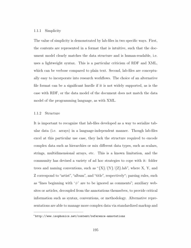
1.1.1 Simplicity
The value of simplicity is demonstrated by lab-files in two specific ways. First,
the contents are represented in a format that is intuitive, such that the doc-
ument model clearly matches the data structure and is human-readable, i.e.
uses a lightweight syntax. This is a particular criticism of RDF and XML,
which can be verbose compared to plain text. Second, lab-files are conceptu-
ally easy to incorporate into research workflows. The choice of an alternative
file format can be a significant hurdle if it is not widely supported, as is the
case with RDF, or the data model of the document does not match the data
model of the programming language, as with XML.
1.1.2 Structure
It is important to recognize that lab-files developed as a way to serialize tab-
ular data (i.e. arrays) in a language-independent manner. Though lab-files
excel at this particular use case, they lack the structure required to encode
complex data such as hierarchies or mix different data types, such as scalars,
strings, multidimensional arrays, etc. This is a known limitation, and the
community has devised a variety of ad hoc strategies to cope with it: folder
trees and naming conventions, such as “{X}/{Y}/{Z}.lab”, where X, Y, and
Z correspond to “artist”, “album”, and “title”, respectively∗; parsing rules, such
as “lines beginning with ‘#’ are to be ignored as comments”; auxiliary web-
sites or articles, decoupled from the annotations themselves, to provide critical
information such as syntax, conventions, or methodology. Alternative repre-
sentations are able to manage more complex data via standardized markup and
∗http://www.isophonics.net/content/reference-annotations
195
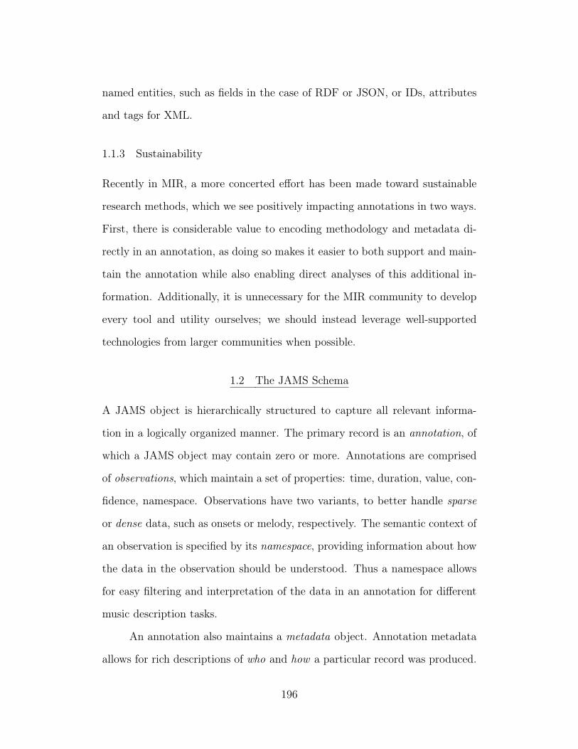
named entities, such as fields in the case of RDF or JSON, or IDs, attributes
and tags for XML.
1.1.3 Sustainability
Recently in MIR, a more concerted effort has been made toward sustainable
research methods, which we see positively impacting annotations in two ways.
First, there is considerable value to encoding methodology and metadata di-
rectly in an annotation, as doing so makes it easier to both support and main-
tain the annotation while also enabling direct analyses of this additional in-
formation. Additionally, it is unnecessary for the MIR community to develop
every tool and utility ourselves; we should instead leverage well-supported
technologies from larger communities when possible.
1.2 The JAMS Schema
A JAMS object is hierarchically structured to capture all relevant informa-
tion in a logically organized manner. The primary record is an annotation, of
which a JAMS object may contain zero or more. Annotations are comprised
of observations, which maintain a set of properties: time, duration, value, con-
fidence, namespace. Observations have two variants, to better handle sparse
or dense data, such as onsets or melody, respectively. The semantic context of
an observation is specified by its namespace, providing information about how
the data in the observation should be understood. Thus a namespace allows
for easy filtering and interpretation of the data in an annotation for different
music description tasks.
An annotation also maintains a metadata object. Annotation metadata
allows for rich descriptions of who and how a particular record was produced.
196
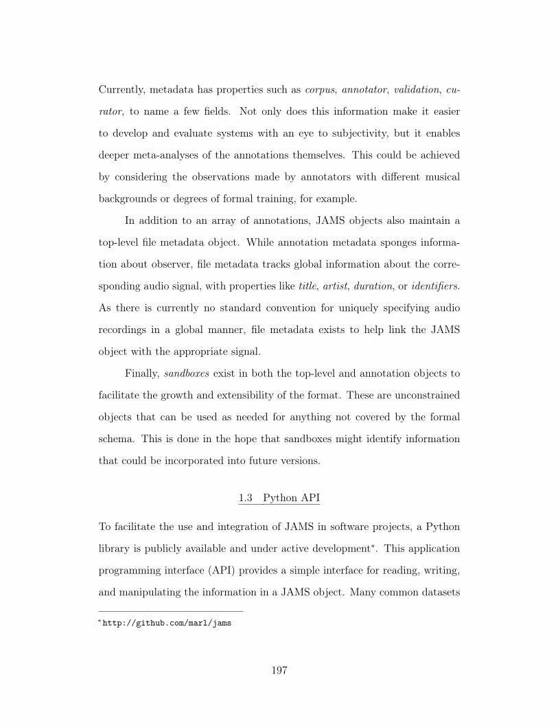
Currently, metadata has properties such as corpus, annotator, validation, cu-
rator, to name a few fields. Not only does this information make it easier
to develop and evaluate systems with an eye to subjectivity, but it enables
deeper meta-analyses of the annotations themselves. This could be achieved
by considering the observations made by annotators with different musical
backgrounds or degrees of formal training, for example.
In addition to an array of annotations, JAMS objects also maintain a
top-level file metadata object. While annotation metadata sponges informa-
tion about observer, file metadata tracks global information about the corre-
sponding audio signal, with properties like title, artist, duration, or identifiers.
As there is currently no standard convention for uniquely specifying audio
recordings in a global manner, file metadata exists to help link the JAMS
object with the appropriate signal.
Finally, sandboxes exist in both the top-level and annotation objects to
facilitate the growth and extensibility of the format. These are unconstrained
objects that can be used as needed for anything not covered by the formal
schema. This is done in the hope that sandboxes might identify information
that could be incorporated into future versions.
1.3 Python API
To facilitate the use and integration of JAMS in software projects, a Python
library is publicly available and under active development∗. This application
programming interface (API) provides a simple interface for reading, writing,
and manipulating the information in a JAMS object. Many common datasets
∗http://github.com/marl/jams
197
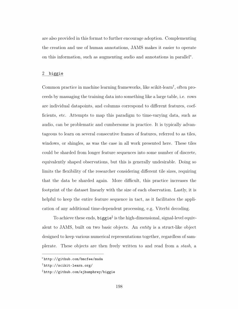
are also provided in this format to further encourage adoption. Complementing
the creation and use of human annotations, JAMS makes it easier to operate
on this information, such as augmenting audio and annotations in parallel∗.
2 biggie
Common practice in machine learning frameworks, like scikit-learn†, often pro-
ceeds by massaging the training data into something like a large table, i.e. rows
are individual datapoints, and columns correspond to different features, coef-
ficients, etc. Attempts to map this paradigm to time-varying data, such as
audio, can be problematic and cumbersome in practice. It is typically advan-
tageous to learn on several consecutive frames of features, referred to as tiles,
windows, or shingles, as was the case in all work presented here. These tiles
could be sharded from longer feature sequences into some number of discrete,
equivalently shaped observations, but this is generally undesirable. Doing so
limits the flexibility of the researcher considering different tile sizes, requiring
that the data be sharded again. More difficult, this practice increases the
footprint of the dataset linearly with the size of each observation. Lastly, it is
helpful to keep the entire feature sequence in tact, as it facilitates the appli-
cation of any additional time-dependent processing, e.g. Viterbi decoding.
To achieve these ends, biggie‡ is the high-dimensional, signal-level equiv-
alent to JAMS, built on two basic objects. An entity is a struct-like object
designed to keep various numerical representations together, regardless of sam-
plerate. These objects are then freely written to and read from a stash, a
∗http://github.com/bmcfee/muda†http://scikit-learn.org/‡http://github.com/ejhumphrey/biggie
198
persistent, i.e. on-disk, key-value store. Here, each entity is given a unique
key, making it easy to align a dictionary of signals with a dictionary of anno-
tations. Leveraging the h5py∗ library under the hood and based on HDF5†,
biggie scales to arbitrarily large datasets; however, though it shares a common
interface with in-memory dictionaries, the footprint of a stash scales grace-
fully with available computational resources by lazily loading data into mem-
ory. Biggie also allows random access and data caching, greatly facilitating
stochastic sampling for on-line learning‡. Perhaps most practically though,
biggie serves as the data interchange format between processing stages in the
larger framework, eliminating the need for filename parsing or content-specific
naming conventions; operations are written to consume and return stashes
with data under the same keys. While biggie helps address similar pain points
as other libraries, like pandas§, the HDF5 back-end is crucial for serializing a
large collection numerical tensors in a simple, Pythonic manner.
3 optimus
Deep learning tools have matured rapidly in the last half decade, with power-
ful choices across several programming languages. Developed under the direc-
tion of Yoshua Bengio at the University of Montreal, Theano¶, is the leading
Python library for deep learning. Boasting a large and growing user base,
Theano offers all the pieces necessary for deep learning research, including
∗http://www.h5py.org/†http://www.hdfgroup.org/HDF5/‡https://github.com/bmcfee/pescador§http://pandas.pydata.org/¶http://deeplearning.net/software/theano/
199
symbolic differentiation, optimized C-implementations, and seamless integra-
tion with GPUs. Though extremely powerful, useful, and expressive, there are
two facets of the library that proved troublesome in the course of this work.
Serialization is can be tricky, especially for networks under active development.
The common approach to saving objects in Python, known as “pickling”, is sen-
sitive to modifications to the code, and thus something pickled previously may
not be recoverable in the future. Additionally, designing neural networks in
Theano can be rather time-consuming, and is not the most user-friendly expe-
rience. This is especially true when constructing non-standard architectures,
such as guitar fretboard models or pairwise training strategies.
Optimus∗ is therefore an effort to address both of these problems in a
maximally versatile and intuitive manner. To simplify the creation, training,
and application of neural networks, common building blocks are provided as
natively serializable objects that can be wired together in a graphical manner.
Arbitrary acyclic, i.e. no loops, directed processing graphs can be architected
from a large collection of nodes, including inputs, functions, like “Affine” or
“Conv3D”, and outputs. While a large space of loss functions can be realized
from these basic building blocks, a handful of standard losses are provided,
simplifying design further. The topology between these parts is given by a
routing table, and passed off to a graph, which connects the dots and returns
a callable function. Furthermore, given the flexibility to define topologies in
a processing graph, it is simple to explore a variety of modifications, such as
layer-wise hyperparameters, tapping various intermediary representations as
outputs, or “cloning” a processing node to create a deep copy of its parameters.
∗http://github.com/ejhumphrey/optimus
200
In addition to the user-facing advantages, robust serialization is achieved
by expressing processing graph definitions as JSON and archives of multidi-
mensional arrays. This offers the additional benefit that it would be straight-
forward to port optimus models, as graph definitions and parameter bundles,
across languages in the future. Finally, as parameter assignments are expressed
through named nodes and fields, it is trivial to not only save parameters but
easily initialize them by arbitrary means, such as pre-training or using super-
vised learning on hand-crafted functions.
4 mir_eval
As addressed at the outset of this work, the conventional formulation of many
music description tasks attempts to model the behavior of an expert human
listener. Framing the problem as a mapping between inputs and outputs allows
for objective quantitative evaluation, thus providing common dimensions on
which to compare algorithms and systems against each other. The particular
dimensions on which an algorithm is evaluated is almost by definition specific
to the application, and different metrics have evolved over time to provide mu-
sically meaningful assessment. Many such scoring functions are nontrivial to
implement, however, and small details can give rise to variability in resulting
metrics. The Music Information Retrieval Evaluation eXchange (MIREX), the
community’s annual algorithm evaluation event, has helped provide common
ground on which to compare different systems. This implementation is seldom
used outside MIREX due to a variety of practical difficulties, however, and in-
stead, researchers often resort to reimplementing the same evaluation metrics.
Unfortunately these personal implementations are not standardized, and may
201
differ in important details, or even contain bugs, confounding comparisons.
Therefore, the mir_eval project aims to address these challenges for a variety
of well-established tasks (Raffel et al., 2014).
Though larger in scope, the contributions to the chord estimation eval-
uation are particularly relevant to this work. Despite being one of the old-
est MIREX tasks, evaluation methodology and metrics for automatic chord
estimation is an ongoing topic of discussion, due to issues with vocabular-
ies, comparison semantics, and other lexicographical challenges unique to the
task (Pauwels & Peeters, 2013). One source of difficulty stems from an in-
herent subjectivity in “spelling” a chord name and the level of detail a human
observer can provide in a reference annotation (Ni et al., 2013). As a result,
a consensus has yet to be reached regarding the single best approach to com-
paring two sequences of chord labels, and instead are often compared over a
set of rules, i.e Root, Major-Minor, and Sevenths, with or without inversions.
To efficiently compare chords, a given chord label is first separated into
its constituent parts, based on the syntax of (Harte, 2010). For example,
the chord label G:maj(6)/5 is mapped to three pieces of information: the
root (“G”), the root-invariant active semitones as determined by the quality
shorthand (“maj”) and scale degrees (“6”), and the bass interval (“5”). Based on
this representation, an estimated chord label can be compare with a reference
by defining a comparison function between these invariant representations.
Any encoded chords that are deemed to be “out of gamut” return a negative
score to be easily filtered. Track-wise scores are computed by weighting each
comparison by the duration of its interval, over all intervals in an audio file.
This is achieved by forming the union of the boundaries in each sequence,
sampling the labels, and summing the time intervals of the “correct” ranges.
202
The cumulative score, referred to as weighted chord symbol recall, is tallied
over a set audio files by discrete summation, where the importance of each
score is weighted by the duration of each annotation (Mauch, 2010).
5 dl4mir
Leveraging these various software components, an aggregate framework repre-
senting all work presented herein is also made available, referred to as dl4mir∗.
At a high level, this resource contains the additional functionality necessary
to reproduce this work. For convenience, the majority of processes can be
executed via a series of shell scripts to perform feature extraction, training,
and evaluation. All reported results and figures provided in this document are
survived in IPython notebooks for both reference and repeatability. Further-
more, dependencies have been minimized to make this framework sufficiently
independent. In addition to the immediate goal of reproducing experimental
results, this is done in the hope that it may facilitate future extensions of this
work. Serialized versions of important network models are also included to
make comparisons against similar work easier, or to simply build them into
other systems. Finally, the source code is provided so that it will serve as an-
other example of how one might architect a flexible deep learning framework.
6 Summary
This chapter has covered the various libraries and programming tools devel-
oped in the course of this work: jams, a JSON format and Python API for
music annotation; biggie, an HDF5 interface for managing large amounts
∗http://github.com/ejhumphrey/dl4mir
203
of numerical data; optimus, a versatile yet intuitive approach to building,
training, and saving deep networks; and mir_eval, an open framework for
evaluation. Not only are many of these components independently useful to
deep learning workflows, but the software necessary to repeat the research
reported here is made publicly available online, in the form of dl4mir. Fol-
lowing the spirit of reproducible research, these efforts aspire to make it easier
to repeat, compare against, and extend the work presented, ultimately serving
the greater music informatics community.
204
CHAPTER VIII
CONCLUSION
This thesis has explored the application of deep learning methods to the
general domain of automatic music description, focusing on timbre similarity
and automatic chord estimation. Encouraging performance is obtained in both
areas, advancing the state of art in the latter, while providing deeper insight
to the tasks at hand. These observations encourage the slight reformulation
of chord estimation as a representation learning, rather than a classification,
problem, resulting in a high performing system with myriad practical bene-
fits. This chapter summarizes the main contributions of this work, and offers
perspectives for the future, including an assessment of outstanding challenges
and the potential impact of continued research in this domain.
1 Summary
Automatic music description is at the heart of content-based music informatics
research. This is necessary for problems where manual annotation does not
scale, such as acoustic similarity, as well as problems where most people lack
the musical expertise to perform the task well, such as transcription. While this
topic is independently valuable, it would seem that progress is decelerating,
and thus any efforts to correct this course must first determine why. In Chapter
II, common practice in automatic music description was revisited, leading to
the identification of three deficiencies worth addressing: hand-crafted feature
205
design is not sustainable, shallow architectures are fundamentally limited, and
short-time analysis alone fails to capture long-term musical structure. Deep
architectures and feature learning were shown to hold promise in music analysis
tasks, evidenced both conceptually and by its growing success, motivating the
exploration of deep learning in automatic music description.
At this point, it was necessary to consider what is “deep learning”, and
why is this an option now? In Chapter III, the history of the field was first
re-examined, showing that after an over-hyped introduction, neural networks
languished through the latter part of the 20th century. This period of skep-
ticism and disinterest gave technology time to catch up to the theory, and
after a serious of significant research contributions, deep learning made a tri-
umphant return to the fore of computer science, toppling longstanding bench-
marks seemingly overnight. While this has brought about a second wave of
hype and interest, it also encouraging the curation of a more established theory
of deep networks. As reviewed, the modern practice of deep learning consists of
a handful of modular processing blocks, strung together in differentiable func-
tions and numerically optimized to an objective function via gradient-based
methods, complemented by a growing suite of practical tricks of the trade.
Having reviewed the modern core of deep learning, this work shifted fo-
cus in Chapter IV to explore these methods directly. As a first inquiry, a deep
convolutional network was applied to the task of timbre similarity, achieving
three goals: the model is able to learn relevant signal-level features that give
rise to source identification; the resulting output space is organized in a se-
mantically meaningful way; and the smoothness of the space is indicated by
error analysis. The approach presented here also offers novel extensions to
previous efforts in pairwise training, achieving extremely robust representa-
206
tions despite a considerable reduction in dimensionality. And perhaps most
importantly, these results are obtained without the need for costly subjective
pairwise ratings of content.
Whereas timbre similarity served as a relatively constrained problem,
Chapter V sought to test the limits of deep learning as applied to automatic
chord estimation, a well-established music informatics challenge. Competitive
performance is achieved with a deep convolutional neural network, evaluated
in both a conventional and large-vocabulary variant of the task. Somewhat
more interestingly, rigorous error analysis reveals that efforts in automatic
chord estimation are converging to a glass ceiling, due in large part to the
objective formulation of an often subjective experience. The problems caused
by the tenuous nature of “ground truth” annotations are exacerbated by efforts
to treat chord estimation as a flat, rather than hierarchical, classification task.
Therefore, the single most critical advancement facing the topic of automatic
chord estimation is a re-evaluation of the task the community is attempting
to solve and the data used to do so.
Despite these difficulties, the chord estimation data is leveraged to ask a
slightly different question: can a model be built to automatically predict chords
as guitar tablature? Therefore, in Chapter VI, again using a deep convolutional
architecture, global performance statistics are improved over the general chord
estimation system, while offering significant practical benefits. In addition to
being a high-performing system, the fretboard estimations are immediately
human-readable and thus attractive from a user experience perspective. Such
a representation is also advantageous from a data collection, correction, and
validation standpoints, significantly reducing the degree of prerequisite skill
necessary to contribute annotations.
207
Finally, the various open source software artifacts developed in the course
of this research are introduced and detailed in Chapter VII: jams, the struc-
tured music annotation format designed for multiplicity of both annotator per-
spective and task namespace; biggie, an approach to managing large collec-
tions of numerical data for training stochastic learning algorithms; optimus, a
user-friendly library for describing and serializing trainable processing graphs;
mir_eval, a suite of evaluation tools for benchmarking music description algo-
rithms; and finally dl4mir, a common framework for the systems and results
presented here.
2 Perspectives on Future Work
Based on the work performed herein and observations made in the process, this
section offers several perspectives on deep learning, music informatics, and the
intersection between them, in the spirit of helping guide future work.
2.1 Architectural Design in Deep Learning
Among the most common questions currently facing the application of deep
learning to any problem is that of architectural design. “How many layers,”
one might ask, “or how many kernels are necessary for this to work? Should
I use convolutions, or matrix products, or something else altogether? And
furthermore, if and when it does actually work, what on earth is it doing?”
Admittedly, the combination of numerical optimization and extremely versa-
tile functions often results in systems with opaque mid-level representations,
earning deep networks the reputation as “black boxes” and the study of them
a “dark art”. However, while these enigmatic functions might cause under-
208
standable confusion, the design of deep architectures is not necessarily devoid
of intuition.
But where to start? The simplest way one might begin to explore deep
learning for some problem of choice is to build some previously published al-
gorithm and use gradient descent to fine-tune the hand crafted weights. There
are countless MIR systems could be reformulated in the deep learning frame-
work, such as onset detection, instrument identification, or pitch estimation.
Most importantly, doing so eliminates the need to compare minor implemen-
tation details, like specific hyperparameters or window coefficients; just learn
it and let it all come out in the wash. Additionally, introducing the process
of learning to classic music informatics systems makes it easier to combine
multiple systems to reap the benefits of model averaging. The key takeaway
here is the notion that good architectures already exist for some problems, and
that better performance can be obtained by using numerical optimization to
expand the space of parameters considered.
Critically, these lessons and practices transcend known problems to new
ones. As demonstrated with the fretboard architecture of Chapter VI, systems
can be quickly constructed by appropriately constraining the behavior. Since
a guitar has six strings, and each can only be active in one place, it makes
sense to model each as a probability surface. That said, there is much more
could be done here. Perhaps transition constraints could be imposed, such
that the model would prefer common chord shapes, or positional constraints,
whereby nearby frets are preferred to large jumps. In this manner, end-to-
end systems can be designed and developed at a high level, and numerical
optimization can be leveraged to work out the fine details. Furthermore, while
learning can discover useful features that were previously overlooked or not
209
considered, this advantage is amplified for new challenges and applications
that do not offer much guiding intuition. For tasks like artist identification or
automatic mixing, it is difficult to comprehend, much less articulate, exactly
what signal attributes are informative to the task and how an implementation
might robustly capture this information.
Thus, deep learning, as an approach to system design, transforms the
challenge from “how do I implement the desired behavior?” to “how do I achieve
the desired behavior?” The nature of this advantage is illustrated by the
relationship between programming in a high-level language, like Python, and
a low-level one, like assembly. Technically speaking, both can be used to the
same ends, but high-level languages allow for faster development of complex
systems by abstracting away the minute details, like memory management or
the laborious task of moving data around registers. In both cases, precise
control is traded for power, leaving the developer to focus on the task at hand
with greater speed and efficiency. Note, however, that abstraction doesn’t
eliminate the need for sound architecture, only the need to worry about certain
facets. The fundamental design challenge is the same, but operating at a higher
level of abstraction allows the deep learning researcher to build bigger systems
faster.
Therefore, it is worthwhile to note that music informatics researchers
are quite proficient at leveraging domain knowledge, engineering acumen, and
a bit of intuition to architect signal processing systems; how many principal
components should one keep of a feature representation? what is a suitable
window size for a Fourier transform? how many subbands should a given
filterbank have? The same intuition can and should be used to design deep
networks, as discussed in the learning of chroma, the design of a tempo es-
210
timation system, or constructing instrument-specific models. Ultimately, the
process of designing a deep architecture is as arbitrary or intentional as one
makes it; it’s only guesswork if you’re guessing.
2.2 Practical Advice for Fellow Practitioners
While the previous discussion hopefully serves to address some of the mystery
inherent to deep learning, it certainly entails the disclaimer of “your mileage
may vary.” The following are a handful of guidelines accumulated in the course
of research; far more suggestion than direction, they have served well in prac-
tice.
1. Data is fundamental: The data-driven researcher will live and die by
the quality of data available. It is widely held that lots of weakly labeled
data will often trump a small amount of strongly labeled data. The
cousin of this sentiment is once you have enough data, everything will
come out in the wash. Take care to note that though this may hold for
training, with caveats, the inverse is true for evaluation. Furthermore,
beware obscure biases in data. Greedy optimization will happily yield
bad solutions because of oversights in the curation of training data. This
is particularly true of regression problems. It is possible to compensate
for biased data in classification via uniform class presentation or like-
lihood scaling, but this can be far less obvious for continuous valued
outputs.
2. Design what you know, learn what you don’t: As mentioned, neu-
ral networks offer the theoretical promise of the universal approximation
theorem, but realizing such general behavior is far from trivial. It is
211
therefore crucial to leverage domain knowledge where possible. This will
typically take two forms: one, simplify the learning problem by remov-
ing degrees of freedom known to be irrelevant to the problem; two, con-
strain the learning problem to encourage musically plausible solutions.
If loudness doesn’t impact one’s ability to recognize chords, for example,
the data should probably be normalized. Music informatics researchers
have a diverse background on which to draw, and this knowledge can be
incorporated into the model or training strategy. Notably, curriculum
learning will likely become a much larger topic in the near future, and
much can be incorporated from music education and pedagogy in this
process.
3. Over-fitting is your friend: Long heralded as the boon of deep net-
works, over-fitting is arguably a good sign, and far more desirable behav-
ior than the inverse. Simply put, if a deep network is unable to over-fit
the training data, something is likely wrong. This is often due to one or
more of the following three issues; one, it is indicative of a problem with
the data, e.g. the observations and targets are uncorrelated or, worse,
conflicting; two, the chosen model lacks the representational power to fit
the training data; or three, and most problematic, the learning problem
is poorly posed and optimization is getting stuck in a bad local minima.
The methods for dealing with such issues are not so well codified, but
consist of data cleaning, exploring “bigger” models, unsupervised pre-
training, changing the loss function, etc.; that said, the efficacy of such
approaches will vary case by case.
4. Get good mileage out of greedy optimization: Gradient descent
212
and other such greedy methods are certainly prone to bad local minima,
but it is not impossible to take active measures to discourage unfortunate
solutions. Additionally, it may be easier to define the kinds of things a
model shouldn’t do than the things it should. For example, a fretboard
prediction network could incorporate a penalty whereby “unplayable”
chord shapes incur significant loss to help keep outputs in a realistic
space.
5. The gap between “real” and synthetic music is closing: As more
modern music transitions to a digital environment, the difference in qual-
ity between a real sound recording and one synthesized for research pur-
poses is converging to zero. Generally speaking, samplers, synthesizers,
and other music production software are underutilized in data-driven
music research. These high quality tools can also be used for data aug-
mentation to make algorithms robust to irrelevant deformations, such as
perceptual codecs, background noise, tempo modulation, or pitch shift-
ing. By generating an unprecedented amount of realistic training data,
can we functionally solve tasks such as onset detection, pitch detection,
or tempo estimation?
2.3 Limitations, Served with a Side of Realism
As some of its forebears recognize and advocate, especially those who perse-
vered through the first AI winter, it is crucial to maintain reasonable expec-
tations for what can be achieved with deep learning. Shown in Figure 47, it is
interesting to consider that, to date, the path of deep learning has roughly fol-
lowed Gartner’s hype cycle for emerging technologies: after a most promising
213
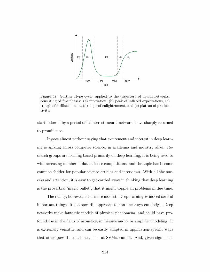
Time1960 1980 2000 2020
Visib
ility
(a) (b) (c) (d) (e)
Figure 47: Gartner Hype cycle, applied to the trajectory of neural networks,consisting of five phases: (a) innovation, (b) peak of inflated expectations, (c)trough of disillusionment, (d) slope of enlightenment, and (e) plateau of produc-tivity.
start followed by a period of disinterest, neural networks have sharply returned
to prominence.
It goes almost without saying that excitement and interest in deep learn-
ing is spiking across computer science, in academia and industry alike. Re-
search groups are forming based primarily on deep learning, it is being used to
win increasing number of data science competitions, and the topic has become
common fodder for popular science articles and interviews. With all the suc-
cess and attention, it is easy to get carried away in thinking that deep learning
is the proverbial “magic bullet”, that it might topple all problems in due time.
The reality, however, is far more modest. Deep learning is indeed several
important things. It is a powerful approach to non-linear system design. Deep
networks make fantastic models of physical phenomena, and could have pro-
found use in the fields of acoustics, immersive audio, or amplifier modeling. It
is extremely versatile, and can be easily adapted in application-specific ways
that other powerful machines, such as SVMs, cannot. And, given significant
214
gains in compute power, the combination of architectural flexibility and nu-
merical optimization makes it an arguably efficient research strategy, at least
more so than graduate students manually tuning parameters.
That said, there are a few important things deep learning is not. It is by
no means the best answer to every problem. Deep learning is, in its current
forms, still relatively data hungry and often computationally expensive. Even
in the case of unsupervised pre-training, sufficient volumes of realistic data
may not be trivial to obtain, as in the case of accelerometers or gyroscopes.
To the latter point, any performance gains obtained with a deep network
could be effectively negated by disproportionate increase in processing time.
Both of these limitations are like to become less important over time, but
remain relevant today. More conceptually, albeit somewhat contentiously, nor
can the modern flavors of deep learning be called “intelligent”; echoing the
ghost of Searle, a system may certainly behave intelligently without truly being
so. Despite the imagery evoked by metaphors and figurative language that
pervade the field, deep learning has as much in common with humanity as a
player piano, and learning is merely a means of programming in a data-driven
manner. This is not to say that deep learning can or will not lead to such
breakthroughs, but care should be taken when differentiating metaphor from
reality.
What should one make of deep learning then? Suffice it to say that deep
learning is just another tool —a powerful tool, but a tool nonetheless— to be
included in the toolbelt of the information science practitioner. Similar to the
trajectories of other, now standard, methods, such as principal components
analysis, Gaussian mixture models, or support vector machines, deep learning
is settling into the final stage of its hype cycle, the point at which it becomes
215
a means to solve a problem. Is deep learning some magic bullet? Of course
not. Is it intelligent? Hardly. But is it useful? Can it accelerate the process
of system design and implementation? Can it allow the clever researcher to
quickly vet ideas and develop complex, robust systems? The answer to all of
these is yes.
2.4 On the Apparent Rise of Glass Ceilings in Music Informatics
One of the motivating factors of this work was to understand and potentially
address the increasing prevalence of diminishing returns in various music de-
scription tasks, like chord estimation, genre classification, or mood prediction.
The main hypothesis resulting from an initial survey was the idea that com-
mon approaches to system design were inadequate, and another approach to
system design, i.e. deep learning, might afford significant performance gains.
However, one of the most significant outcomes of this work is in some sense
the most unexpected: subtle deficiencies in methodology may be contributing
as much or more to unsatisfactory results than the algorithms or approaches
used to achieve them.
This finding reflects a small but growing trend in music informatics of
critically assessing how the scientific method is applied to machine listening
tasks, with meta-analyses of genre recognition (Sturm, 2014a), rhythmic sim-
ilarity (Esparza, Bello, & Humphrey, 2014), and music segmentation (Nieto,
2015), to name a few. Looking to the intersection of these areas, the research
methodology of automatic music description consists of five basic steps:
1. Define the problem.
2. Collect data.
216
3. Build a solution.
4. Evaluate the model.
5. Iterate.
With this method as a common underpinning, the evolution of content-
based music informatics unfolds logically. Though a young field, the majority
of current research has converged to a handful of established tasks, as evi-
denced by those conducted at MIREX. Labeled music data is notorious diffi-
cult to amass in large quantities, but resources have grown steadily for those
well-worn problems. In cases where it has not, researchers are faced with one
of two options: curate the data themselves, or adapt an existing dataset to
their problem. Having developed a solution, it is necessary to benchmark a
proposed algorithm against previous efforts. However, to make such compar-
isons fairly, it is typically necessary to compute the same metrics over the same
data, as the systems themselves are seldom made public. Thus, most research
efforts today focus almost exclusively on (3) and (5), adopting or otherwise
accepting the other three.
It is critical to note, though, that these other methodological stages —
problem formulation, data curation, and evaluation— have developed natu-
rally over time at the community level, based not on globally optimal design
but rather a combination of evolving understanding, inertia, and convenience.
At this point, it serves to return to an initial question posed by this work:
why are music description systems yielding diminishing returns? The findings
of this work, particularly in the space of automatic chord estimation, corrobo-
rate the growing trend that perhaps the biggest problem facing content-based
music informatics is one of methodology.
217
With this in mind, reconsider the case of automatic chord estimation.
What is the scope of the problem being addressed? “Can an agent provide ac-
ceptable chord transcriptions?” is a very different question from “Can an agent
reproduce these chord transcriptions?” Analysis of the Rock Corpus transcrip-
tions showed that comparing the outputs of two expert musicians can achieve
a “yes” and “no” respectively. Does the data reflect these requirements? Chord
annotations consist of single perspectives from several anonymized annotators.
It is doubtful that all annotators are using the chord labels the same way. How
do we know when the problem is solved? Does weighted chord symbol recall
with different comparison rules correspond to subjective experience? Not all
substitutions are equal, as the distance in harmonic function between a I:7
and a I is quite different from a V:7 and a V, for example.
Understandably, it is easy to lose sight of the fact that research is not
just the process of iterative system development, but the entire arc of the
scientific method. At this point in the trajectory of music informatics, it is
conceivable that several well-worn tasks could use a reassessment of what con-
stitutes methodological best practices. This is hardly a novel realization, but
one that warrants greater awareness within the music informatics community.
It is necessary, but ultimately insufficient, to tirelessly pursue better solutions;
we must be as diligent in our pursuit of better problems.
218
BIBLIOGRAPHY
Andén, J., & Mallat, S. (2011). Multiscale scattering for audio classification.In Proceedings of the 12th international society of music informationretrieval conference (ISMIR). 26
Anglade, A., Ramirez, R., & Dixon, S. (2009). Genre classification usingharmony rules induced from automatic chord transcriptions. In Pro-ceedings of the 10th international society of music information retrievalconference (ISMIR) (pp. 669–674). 116
Barbancho, A., Klapuri, A., Tardón, L. J., & Barbancho, I. (2012). Automatictranscription of guitar chords and fingering from audio. Transactions onAudio, Speech & Language Processing , 20 (3), 915–921. 179
Barrington, L., Yazdani, M., Turnbull, D., & Lanckriet, G. R. (2008). Combin-ing feature kernels for semantic music retrieval. In Proceedings of the 9thinternational society of music information retrieval conference (ISMIR)(pp. 614–619). 75
Bello, J. P. (2007). Audio-based cover song retrieval using approximate chordsequences: Testing shifts, gaps, swaps and beats. In Proceedings of the8th international society of music information retrieval conference (IS-MIR) (pp. 239–244). 116
Bello, J. P., Daudet, L., Abdallah, S., Duxbury, C., Davies, M., & Sandler, M.(2005). A tutorial on onset detection in music signals. IEEE Transactionson Audio, Speech and Language Processing , 13 (5), 1035–1047. 24
Bengio, Y. (2009). Learning deep architectures for AI. Foundations and Trendsin Machine Learning , 2 (1), 1–127. 20, 64
Bengio, Y. (2012). Practical recommendations for gradient-based training of
219
deep architectures. In Neural networks: Tricks of the trade (pp. 437–478). Springer. 63
Bengio, Y., Courville, A., & Vincent, P. (2013). Representation learning:A review and new perspectives. Transactions on Pattern Analysis andMachine Intelligence, 35 (8), 1798–1828. 66
Bengio, Y., & LeCun, Y. (2007). Scaling learning algorithms towards AI.Large-Scale Kernel Machines , 34 . 53
Berenzweig, A., Logan, B., Ellis, D. P., & Whitman, B. (2004). A large-scale evaluation of acoustic and subjective music-similarity measures.Computer Music Journal , 28 (2), 63–76. 17
Bergstra, J., Breuleux, O., Bastien, F., Lamblin, P., Pascanu, R., Desjardins,G., . . . Bengio, Y. (2010, June). Theano: a CPU and GPU mathexpression compiler. In Proceedings of the of the python for scientificcomputing conference (SciPy). 45
Bertin-Mahieux, T., Ellis, D. P., Whitman, B., & Lamere, P. (2011). Themillion song dataset. In Proceedings of the 11th international society ofmusic information retrieval conference (ISMIR) (pp. 591–596). 32, 194
Bertin-Mahieux, T., & Ellis, D. P. W. (2012). Large-scale cover song recog-nition using the 2D Fourier transform magnitude. In Proceedings ofthe 13th international society of music information retrieval conference(ISMIR) (p. 241-246). 14
Bishop, C. (2006). Pattern recognition and machine learning. Springer. 17,18, 59
Bittner, R., Salamon, J., Tierney, M., Mauch, M., Cannam, C., & Bello, J.(2014). Medleydb: a multitrack dataset for annotation-intensive mirresearch. In Proceedings of the 15th international society of music infor-mation retrieval conference (ISMIR). 32
Boulanger-Lewandowski, N., Bengio, Y., & Vincent, P. (2013). Audio chordrecognition with recurrent neural networks. In Proceedings of the 14th
220
international society of music information retrieval conference (ISMIR)(pp. 335–340). 30
Bregman, A. S. (1994). Auditory scene analysis: The perceptual organizationof sound. MIT press. 71
Brumfiel, G. (2014). Deep learning: Teaching computers to tellthings apart. Retrieved 2015-04-20, from http://www.npr.org/
blogs/alltechconsidered/2014/02/20/280232074/deep-learning
-teaching-computers-to-tell-things-apart 24
Burgoyne, J. A., & Saul, L. K. (2005). Learning harmonic relationships indigital audio with dirichlet-based hidden markov models. In Proceedingsof the 6th international society of music information retrieval conference(ISMIR) (pp. 438–443). 121
Burgoyne, J. A., Wild, J., & Fujinaga, I. (2011). An expert ground truthset for audio chord recognition and music analysis. In Proceedings ofthe 11th international society of music information retrieval conference(ISMIR) (pp. 633–638). 123, 193
Cabral, G., & Pachet, F. (2006). Recognizing chords with EDS: Part One.Computer Music Modeling and Retrieval , 185–195. 121
Caclin, A., McAdams, S., Smith, B. K., & Winsberg, S. (2005). Acoustic cor-relates of timbre space dimensions: A confirmatory study using synthetictonesa). Journal of the Acoustical Society of America, 118 (1), 471–482.74
Cannam, C., Landone, C., Sandler, M. B., & Bello, J. P. (2006). The sonicvisualiser: A visualisation platform for semantic descriptors from mu-sical signals. In Proceedings of the 7th international society of musicinformation retrieval conference (ISMIR) (pp. 324–327). 194
Casey, M., Rhodes, C., & Slaney, M. (2008). Analysis of minimum distancesin high-dimensional musical spaces. Transactions on Audio, Speech, andLanguage Processing , 16 (5), 1015–1028. 22
221
Casey, M., Veltkamp, R., Goto, M., Leman, M., Rhodes, C., & Slaney, M.(2008). Content-based music information retrieval: Current directionsand future challenges. Proceedings of the IEEE , 96 (4), 668–696. 13
Cateforis, T. (2002). How alternative turned progressive: The strange case ofmath rock. Progressive Rock Reconsidered , 243–260. 117
Cho, T. (2014). Improved techniques for automatic chord recognition frommusic audio signals (Unpublished doctoral dissertation). New York Uni-versity. 27, 119, 121, 122, 124, 126, 139, 142, 150, 185, 187
Cho, T., & Bello, J. P. (2011). A feature smoothing method for chord recog-nition using recurrence plots. In Proceedings of the 12th internationalsociety of music information retrieval conference (ISMIR). 121
Cho, T., Kim, K., & Bello, J. P. (2012). A minimum frame error criterionfor hidden markov model training. In 11th international conference onmachine learning and applications (icmla) (Vol. 2, pp. 363–368). 122
Cho, T., Weiss, R. J., & Bello, J. P. (2010). Exploring common variations instate of the art chord recognition systems. In Proceedings of the soundand music computing conference. 18, 121, 122, 128, 131
Chordia, P., Sastry, A., & Sentürk, S. (2011). Predictive tabla modellingusing variable-length markov and hidden markov models. Journal ofNew Music Research, 40 (2), 105-118. 16, 122
Coates, A., & Ng, A. Y. (2012). Learning feature representations with k-means. In Neural networks: Tricks of the trade (pp. 561–580). Springer.50
Collobert, R., Kavukcuoglu, K., & Farabet, C. (2011). Torch7: A matlab-likeenvironment for machine learning. In Biglearn, nips workshop. 45
Cybenko, G. (1989). Approximation by superpositions of a sigmoidal function.Mathematics of control, signals and systems , 2 (4), 303–314. 38
Dahl, G. E., Yu, D., Deng, L., & Acero, A. (2012). Context-dependent pre-
222
trained deep neural networks for large-vocabulary speech recognition.Transactions on Audio, Speech, and Language Processing , 20 (1), 30–42.149
Dannenberg, R. (1984). An on-line algorithm for real-time accompaniment.In Proceedings of the international computer music conference (ICMC)(pp. 193–198). 24
Davis, S., & Mermelstein, P. (1980). Comparison of parametric represen-tations for monosyllabic word recognition in continuously spoken sen-tences. Transactions on Acoustics, Speech and Signal Processing , 28 (4),357–366. 75
Dean, J., Corrado, G., Monga, R., Chen, K., Devin, M., Mao, M., . . . others(2012). Large scale distributed deep networks. In Advances in neuralinformation processing systems (nips) (pp. 1223–1231). 45
De Clercq, T., & Temperley, D. (2011). A corpus analysis of rock harmony.Popular Music, 30 (01), 47–70. 162
De Haas, W. B., & Burgoyne, J. A. (2012). Parsing the billboard chordtranscriptions. University of Utrecht, Technical Report . 193
Deng, J., Dong, W., Socher, R., Li, L.-J., Li, K., & Fei-Fei, L. (2009). Ima-genet: A large-scale hierarchical image database. In Computer vision andpattern recognition, 2009. cvpr 2009. ieee conference on (pp. 248–255).43
Dieleman, S., Brakel, P., & Schrauwen, B. (2011). Audio-based music clas-sification with a pretrained convolutional network. In Proceedings ofthe 12th international society of music information retrieval conference(ISMIR). 30
Dixon, S. (2007). Evaluation of the audio beat tracking system Beatroot.Journal of New Music Research, 36 (1), 39–50. 25
Donnadieu, S. (2007). Mental representation of the timbre of complex sounds.In Analysis, synthesis, and perception of musical sounds (pp. 272–319).
223
Springer. 71
Edward, W., & Kolen, J. F. (1994). Resonance and the perception of musicalmeter. Connection Science, 6 (2-3), 177–208. 25
Esparza, T. M., Bello, J. P., & Humphrey, E. J. (2014). From genre classifi-cation to rhythm similarity: Computational and musicological insights.Journal of New Music Research, 1–19. 216
Essid, S., Richard, G., & David, B. (2006). Musical Instrument Recognition byPairwise Classification Strategies. IEEE Transactions on Audio, Speechand Language Processing , 14 (4), 1401–1412. 75
Fisher, W. M., Doddington, G. R., & Goudie-Marshall, K. M. (1986). Thedarpa speech recognition research database: Specifications and status.(Tech. Rep.). 43
Flexer, A., Schnitzer, D., & Schlueter, J. (2012). A MIREX meta-analysisof hubness in audio music similarity. In Proceedings of the 13th in-ternational society of music information retrieval conference (ISMIR)(p. 175-180). 15
Fujishima, T. (1999). Realtime chord recognition of musical sound: a systemusing common lisp music. In Proceedings of the international computermusic conference (ICMC). 27, 120
Fukushima, K. (1988). Neocognitron: A hierarchical neural network capableof visual pattern recognition. Neural Networks . 41
Glennon, A. (2014). Evolving synthesis algorithms using a measure of tim-bre sequence similarity (Unpublished doctoral dissertation). New YorkUniversity. 73
Goto, M., & Muraoka, Y. (1995). A real-time beat tracking system for audiosignals. In Proceedings of the international computer music conference(ICMC) (pp. 171–174). 25
Grey, J. M. (1977). Multidimentional perceptual scaling of musical timbre.
224
Journal Acoustical Society of America, 61 , 1270–1277. 72
Grosche, P., & Müller, M. (2011). Extracting predominant local pulse infor-mation from music recordings. IEEE Transactions on Audio, Speech andLanguage Processing , 19 (6), 1688–1701. 25
Hadsell, R., Chopra, S., & LeCun, Y. (2006). Dimensionality reduction bylearning an invariant mapping. In Proceedings of the computer visionand pattern recognition conference (cvpr). IEEE Press. 83
Hamel, P., Lemieux, S., Bengio, Y., & Eck, D. (2011). Temporal pooling andmultiscale learning for automatic annotation and ranking of music audio.In Proceedings of the 12th international society of information retrievalconference (ISMIR). 54
Hamel, P., Wood, S., & Eck, D. (2009). Automatic identification of instru-ment classes in polyphonic and poly-instrument audio. In Proceedings ofthe 10th international society of music information retrieval conference(ISMIR). 30
Harte, C. (2010). Towards automatic extraction of harmony information frommusic signals (Unpublished doctoral dissertation). Department of Elec-tronic Engineering, Queen Mary, University of London. 110, 124, 202
Harte, C., Sandler, M. B., Abdallah, S. A., & Gómez, E. (2005). Symbolic rep-resentation of musical chords: A proposed syntax for text annotations.In Proceedings of the 6th international society of music information re-trieval conference (ISMIR) (Vol. 5, pp. 66–71). 113
Henaff, M., Jarrett, K., Kavukcuoglu, K., & LeCun, Y. (2011). Unsupervisedlearning of sparse features for scalable audio classification. In Proceedingsof the 12th international society of music information retrieval confer-ence(ISMIR). 31
Herrera-Boyer, P., Peeters, G., & Dubnov, S. (2003). Automatic classificationof musical instrument sounds. Journal of New Music Research, 32 (1),3–21. 75
225
Hinton, G., Deng, L., Yu, D., Dahl, G., Mohamed, A.-r., Jaitly, N., . . . Kings-bury, B. (2012). Deep neural networks for acoustic modeling in speechrecognition. IEEE Signal Processing Magazine. 23, 24, 45
Hinton, G. E. (1986). Learning distributed representations of concepts. InProceedings of the 8th conference of the cognitive science society (Vol. 1,p. 12). 40
Hinton, G. E., Osindero, S., & Teh, Y. (2006). A fast learning algorithm fordeep belief nets. Neural Computation, 18 (7), 1527–1554. 44, 65
Hinton, G. E., Srivastava, N., Krizhevsky, A., Sutskever, I., & Salakhutdinov,R. R. (2012). Improving neural networks by preventing co-adaptationof feature detectors. arXiv preprint arXiv:1207.0580 . 66, 68
Hori, G., Kameoka, H., & Sagayama, S. (2013). Input-output hmm applied toautomatic arrangement for guitars. Information and Media Technologies ,8 (2), 477–484. 179
Hornik, K. (1991). Approximation capabilities of multilayer feedforward net-works. Neural networks , 4 (2), 251–257. 38
Huang, G. B., Ramesh, M., Berg, T., & Learned-Miller, E. (2007, October).Labeled faces in the wild: A database for studying face recognition inunconstrained environments (Tech. Rep. No. 07-49). University of Mas-sachusetts, Amherst. 43
Hubel, D. H., & Wiesel, T. N. (1959). Receptive fields of single neurones inthe cat’s striate cortex. The Journal of Physiology , 148 (3), 574–591. 41
Humphrey, E. J., & Bello, J. P. (2012). Rethinking automatic chord recogni-tion with convolutional neural networks. In Proceedings of the interna-tional conference on machine learning and applications. 30, 127
Humphrey, E. J., & Bello, J. P. (2014). From music audio to chord tablature:Teaching deep convolutional networks toplay guitar. In Internationalconference on acoustics, speech and signal processing (icassp) (pp. 6974–6978). 179
226
Humphrey, E. J., Bello, J. P., & LeCun, Y. (2012). Moving Beyond FeatureDesign: Deep Architectures and Automatic Feature Learning in MusicInformatics. In Proceedings of the 13th international society of musicinformation retrieval conference (ISMIR). 15
Humphrey, E. J., Cho, T., & Bello, J. P. (2012). Learning a robust tonnetz-space transform for automatic chord recognition. In International con-ference on acoustics, speech and signal processing (icassp). 30, 121, 122
Humphrey, E. J., Glennon, A. P., & Bello, J. P. (2011). Non-linear semanticembedding for organizing large instrument sample libraries. In Interna-tional conference on machine learning and applications (icmla) (Vol. 2,pp. 142–147). 30, 82, 87
Iverson, P., & Krumhansl, C. L. (1993). Isolating the dynamic attributes ofmusical timbrea). Journal of the Acoustical Society of America, 94 (5),2595–2603. 73
Jehan, T. (2005). Creating Music by Listening (Unpublished doctoral disser-tation). Massachusetts Institute of Technology. 76
Ji, S., & Ye, J. (2008). Generalized linear discriminant analysis: a unifiedframework and efficient model selection. IEEE Transactions on NeuralNetworks , 19 (10), 1768–1782. 90
Juang, B.-H., Hou, W., & Lee, C.-H. (1997). Minimum classification errorrate methods for speech recognition. Transactions on Speech and AudioProcessing , 5 (3), 257–265. 60
Kavukcuoglu, K., Sermanet, P., Boureau, Y., Gregor, K., Mathieu, M., &LeCun, Y. (2010). Learning convolutional feature hierachies for vi-sual recognition. In Advances in neural information processing systems(nips). 62, 68
Klapuri, A., & Davy, M. (2006). Signal processing methods for music tran-scription. Springer. 13
Klapuri, A. P., Eronen, A. J., & Astola, J. T. (2006). Analysis of the meter
227
of acoustic musical signals. IEEE Transactions on Audio, Speech andLanguage Processing , 14 (1), 342–355. 24
Krizhevsky, A., Sutskever, I., & Hinton, G. E. (2012). Imagenet classifica-tion with deep convolutional neural networks. In Advances in neuralinformation processing systems (pp. 1097–1105). 23, 45
Krumhansl, C. L. (1979). The psychological representation of musical pitchin a tonal context. Cognitive Psychology , 11 (3), 346–374. 105
Lacoste, A., & Eck, D. (2007). A supervised classification algorithm for noteonset detection. EURASIP Journal on Applied Signal Processing , 2007 ,1–13. doi: 10.1155/2007/43745 30
Laitz, S. G., & Bartlette, C. (2009). Graduate review of tonal theory: Arecasting of common-practice harmony, form, and counterpoint.109
Le, Q., Monga, R., Devin, M., Corrado, G., Chen, K., Ranzato, M., . . . Ng, A.(2012). Building high-level features using large scale unsupervised learn-ing. Proceedings of the International Conference on Machine Learning(ICML). 46
Le, Q. V., Ngiam, J., Chen, Z., Chia, D., Koh, P. W., & Ng, A. Y. (2010).Tiled convolutional neural networks. Advances in Neural InformationProcessing Systems (NIPS), 23 . 49
LeCun, Y., Bottou, L., Bengio, Y., & Haffner, P. (1998). Gradient-basedlearning applied to document recognition. Proceedings of the IEEE ,86 (11), 2278–2324. 42, 55, 182
LeCun, Y., Chopra, S., Hadsell, R., Ranzato, M., & Huang, F. (2006). Atutorial on energy-based learning. Predicting Structured Data. 57
LeCun, Y., Cortes, C., & Burges, C. J. (1998). Mnist handwritten digitdatabase. Retrieved 2015-04-20, from http://yann.lecun.com/exdb/
mnist/index.html 43
228
LeCun, Y. A., Bottou, L., Orr, G. B., & Müller, K.-R. (1998). Efficientbackprop. In Neural networks: Tricks of the trade. Springer. 40
Lee, K., & Slaney, M. (2007). A unified system for chord transcription andkey extraction using hidden markov models. In Proceedings of the 8thinternational society of music information retrieval conference (ISMIR)(pp. 245–250). 121
Levy, M., Noland, K., & Sandler, M. (2007). A comparison of timbral andharmonic music segmentation algorithms. In International conference onacoustics, speech and signal processing (icassp) (Vol. 4, pp. IV–1433). 27
Lewis, D. D., Yang, Y., Rose, T. G., & Li, F. (2004). Rcv1: A new benchmarkcollection for text categorization research. Journal of Machine LearningResearch, 5 , 361–397. 43
Li, T., Chan, A., & Chun, A. (2010). Automatic musical pattern featureextraction using convolutional neural network. In Proceedings of theimecs. 30
Liu, D. C., & Nocedal, J. (1989). On the limited memory bfgs method forlarge scale optimization. Mathematical programming , 45 (1-3), 503–528.62
Logan, B. (2000). Mel frequency cepstral coefficients for music modeling.In Proceedings of the 1st international symposium of music informationretrieval (ISMIR). 75
Lyon, R., Rehn, M., Bengio, S., Walters, T., & Chechik, G. (2010). Soundretrieval and ranking using sparse auditory representations. Neural com-putation, 22 (9), 2390–2416. 18
Maas, A. L., Hannun, A. Y., & Ng, A. Y. (2013). Rectifier nonlinearities im-prove neural network acoustic models. In Proceedings of the internationalconference on machine learning (ICML) (Vol. 30). 53
Mandel, M., & Ellis, D. (2005). Song-level features and support vector ma-chines for music classification. In Proceedings of the 6th international
229
society of music information retrieval conference (ISMIR). 16
Manoury, P. (1991). Les limites de la notion de ‘timbre’. Le timbre: Métaphorepour la composition, 293–299. 71
Markoff, J. (2012). Scientists see promise in deep-learning programs.Retrieved 2015-04-20, from http://www.nytimes.com/2012/11/24/
science/scientists-see-advances-in-deep-learning-a-part-of
-artificial-intelligence.html 24
Mauch, M. (2010). Automatic chord transcription from audio using compu-tational models of musical context (Unpublished doctoral dissertation).School of Electronic Engineering and Computer Science Queen Mary,University of London. 203
Mauch, M., & Dixon, S. (2010a). Approximate note transcription for theimproved identification of difficult chords. In Proceedings of the 11thinternational society of information retrieval conference (ISMIR). 16,122
Mauch, M., & Dixon, S. (2010b). Simultaneous Estimation of Chords andMusical Context From Audio. IEEE Transactions on Audio, Speech andLanguage Processing , 18 (6), 1280–1289. 121, 139
Mauch, M., Noland, K., & Dixon, S. (2009). Using musical structure toenhance automatic chord transcription. In Proceedings of the 10th inter-national society of music information retrieval conference (pp. 231–236).194
McAdams, S., Winsberg, S., Donnadieu, S., De Soete, G., & Krimphoff, J.(1995). Perceptual scaling of synthesized musical timbres: Common di-mensions, specificities, and latent subject classes. Psychological research,58 (3), 177–192. 72
McCulloch, W. S., & Pitts, W. (1943). A logical calculus of the ideas immanentin nervous activity. The bulletin of mathematical biophysics , 5 (4), 115–133. 35
230
McKay, C., Fiebrink, R., McEnnis, D., Li, B., & Fujinaga, I. (2005). Ace: Aframework for optimizing music classification. In Proceedings of the 6thinternational society of music information retrieval conference (ISMIR)(pp. 42–49). 194
McVicar, M. (2013). A Machine Learning Approach to Automatic ChordExtraction (Unpublished doctoral dissertation). University of Bristol.110, 119, 124
Minsky, M., & Papert, S. (1969). Perceptrons. MIT press. 37
Mohamed, A.-r., Sainath, T. N., Dahl, G., Ramabhadran, B., Hinton, G. E.,& Picheny, M. A. (2011). Deep belief networks using discriminativefeatures for phone recognition. In Acoustics, speech and signal processing(icassp), 2011 ieee international conference on (pp. 5060–5063). 20
Müller, M., Ellis, D. P. W., Klapuri, A., & Richard, G. (2011). Signal pro-cessing for music analysis. Journal Selected Topics in Signal Processing ,5 (6), 1088–1110. 13
Müller, M., & Ewert, S. (2010, March). Towards Timbre-Invariant Au-dio Features for Harmony-Based Music. IEEE Transactions on Au-dio, Speech and Language Processing , 18 (3), 649–662. doi: 10.1109/TASL.2010.2041394 121
Müller, M., & Ewert, S. (2011). Chroma Toolbox: MATLAB implementationsfor extracting variants of chroma-based audio features. In Proceedings ofthe 12th international society of music information retrieval conference(ISMIR). Miami, USA. 18
Nam, J., Herrera, J., Slaney, M., & Smith, J. (2012). Learning sparse featurerepresentations for music annotation and retrieval. In Proceedings of the13th international society of information retrieval conference (ISMIR).31
Nam, J., Ngiam, J., Lee, H., & Slaney, M. (2011). A classification-basedpolyphonic piano transcription approach using learned feature represen-tations. In Proceedings of the 12th international society of music infor-
231
mation retrieval conference (ISMIR). 30
Ni, Y., McVicar, M., Santos-Rodriguez, R., & De Bie, T. (2012). An end-to-end machine learning system for harmonic analysis of music. Trans-actions on Audio, Speech, and Language Processing , 20 (6), 1771–1783.139
Ni, Y., McVicar, M., Santos-Rodriguez, R., & De Bie, T. (2013). Under-standing effects of subjectivity in measuring chord estimation accuracy.Transactions on Audio, Speech, and Language Processing , 21 (12), 2607–2615. 171, 193, 202
Nieto, O. (2015). Discovering structure in music: Automatic approaches andperceptual evaluations (Unpublished doctoral dissertation). New YorkUniversity. 216
of Music Merchants, N. A. (2014). The 2014 namm global report. https://
www.namm.org/files/ihdp-viewer/global-report-2014/. 176
Olazaran, M. (1996). A sociological study of the official history of the percep-trons controversy. Social Studies of Science, 26 (3), 611–659. 37
Oudre, L., Grenier, Y., & Févotte, C. (2009). Template-based chord recog-nition: Influence of the chord types. In Proceedings of the 10th inter-national society of music information retrieval conference (ISMIR) (pp.153–158). 121
Page, L., Brin, S., Motwani, R., & Winograd, T. (1999). The pagerank citationranking: Bringing order to the web.2
Papadopoulos, H., & Peeters, G. (2011). Joint estimation of chords anddownbeats from an audio signal. Transactions on Audio, Speech, andLanguage Processing , 19 (1), 138–152. 193
Paulus, J., Müller, M., & Klapuri, A. (2010). State of the art report: Audio-based music structure analysis. In Proceedings of the 11th internationalsociety of music information retrieval conference (ISMIR) (pp. 625–636).
232
75
Pauwels, J., & Peeters, G. (2013). Evaluating automatically estimated chordsequences. In International conference on acoustics, speech and signalprocessing (ICASSP) (pp. 749–753). 202
Plomp, R. (1976). Aspects of tone sensation: a psychophysical study. AcademicPress. 72
Raffel, C., McFee, B., Humphrey, E. J., Salamon, J., Nieto, O., Liang, D.,& Ellis, D. P. (2014). mir_ eval: A transparent implementation ofcommon mir metrics. In Proceedings of the 15th international society ofmusic information retrieval conference. 125, 202
Rosenblatt, F. (1958). The perceptron: a probabilistic model for informationstorage and organization in the brain. Psychological review , 65 (6), 386.35
Salamon, J., Serra, J., & Gómez, E. (2013). Tonal representations for musicretrieval: from version identification to query-by-humming. InternationalJournal of Multimedia Information Retrieval , 2 (1), 45–58. 27
Scheirer, E. D. (1998). Tempo and beat analysis of acoustic musical signals.Journal Acoustical Society of America, 103 (1), 588–601. 24
Schluter, J., & Bock, S. (2014). Improved musical onset detection with con-volutional neural networks. In Acoustics, speech and signal processing(icassp), 2014 ieee international conference on (pp. 6979–6983). 30
Schmidt, E. M., & Kim, Y. E. (2010). Prediction of time-varying musical mooddistributions from audio. In Proceedings of the 11th international societyof music information retrieval conference (ISMIR) (pp. 465–470). 75
Schmidt, E. M., & Kim, Y. E. (2011). Modeling the acoustic structure ofmusical emotion with deep belief networks. In Proceedings of the neuralinformation processing systems. 30
Sermanet, P., Chintala, S., & LeCun, Y. (2012). Convolutional neural networks
233
applied to house numbers digit classification. In International conferenceon pattern recognition (icpr) (pp. 3288–3291). 54
Sermanet, P., Kavukcuoglu, K., Chintala, S., & LeCun, Y. (2013). Pedestriandetection with unsupervised multi-stage feature learning. In Conferenceon computer vision and pattern recognition (cvpr) (pp. 3626–3633). 68
Shannon, C. (1938). A symbolic analysis of relay and switching circuits.Transactions American Institute of Electrical Engineers . 35
Sheh, A., & Ellis, D. P. W. (2003). Chord segmentation and recognition usingem-trained hidden markov models. In Proceedings of the 4th interna-tional society of information retrieval conference (ISMIR). 122
Sigtia, S., Benetos, E., Cherla, S., Weyde, T., Garcez, A. S. d., & Dixon, S.(2014). An rnn-based music language model for improving automaticmusic transcription. In Proceedings of the 15th international society ofmusic information retrieval conference (ISMIR). 31
Slaney, M. (2011). Web-scale multimedia analysis: does content matter?Multimedia, IEEE , 18 (2), 12–15. 15
Sonn, Martin. (1973). American national standard psychoacoustical terminol-ogy (Tech. Rep. No. S3:20). New York: American National StandardsInstitute (ANSI). 70
Sturm, B. L. (2014a). A simple method to determine if a music informationretrieval system is a “horse”. Transactions on Multimedia, 16 (6), 1636–1644. 216
Sturm, B. L. (2014b). The state of the art ten years after a state of the art:Future research in music information retrieval. Journal of New MusicResearch, 43 (2), 147–172. 15
Sturm, B. L., & Collins, N. (2014). The kiki-bouba challenge: Algorithmiccomposition for content-based MIR research and development. In Pro-ceedings of the 15th international society of music information retrievalconference (ISMIR) (pp. 21–26). 15
234
Sumi, K., Arai, M., Fujishima, T., & Hashimoto, S. (2012). A music retrievalsystem using chroma and pitch features based on conditional randomfields. In International conference on acoustics, speech and signal pro-cessing (icassp) (pp. 1997–2000). 16, 122
Sutskever, I., Martens, J., Dahl, G., & Hinton, G. (2013). On the importanceof initialization and momentum in deep learning. In Proceedings of theinternational conference on machine learning (ICML) (pp. 1139–1147).62
Sutskever, I., Martens, J., & Hinton, G. (2011). Generating text with recur-rent neural networks. In Proceedings of the international conference onmachine learning (icml). 45
Szegedy, C., Liu, W., Jia, Y., Sermanet, P., Reed, S., Anguelov, D., . . . Ra-binovich, A. (2014). Going deeper with convolutions. arXiv preprintarXiv:1409.4842 . 47
Tagg, P. (1982). Analysing popular music: theory, method and practice.Popular music, 2 , 37–67. 117
Terasawa, H., Slaney, M., & Berger, J. (2005). The thirteen colors of timbre.Workshop on Applications of Signal Processing to Audio and Acoustics ,323–326. 76
Turing, A. M. (1936). On computable numbers, with an application to theentscheidungsproblem. Journal of Math, 58 (345-363), 5. 34
Turing, A. M. (1950). Computing machinery and intelligence. Mind , 433–460.6
Tzanetakis, G., & Cook, P. (2002). Musical genre classification of audio signals.Speech and Audio Processing, IEEE transactions on, 10 (5), 293–302. 75
Ullrich, K., Schlüter, J., & Grill, T. (2014). Boundary detection in musicstructure analysis using convolutional neural networks. In Proceedings ofthe 15th international society of music information retrieval conference(ISMIR). 30
235
Vaidyanathan, P. P. (1993). Multirate systems and filter banks. PearsonEducation India. 29
Vincent, E., Raczynski, S. A., Ono, N., Sagayama, S., et al. (2010). A roadmaptowards versatile mir. In Proceedings of the 11th international society ofmusic information retrieval conference (pp. 662–664). 193
Von Ahn, L., Blum, M., Hopper, N. J., & Langford, J. (2003). Captcha: Usinghard ai problems for security. In Advances in cryptology (pp. 294–311).Springer. 43
Weller, A., Ellis, D. P. W., & Jebara, T. (2009). Structured prediction modelsfor chord transcription of music audio. In Machine learning and appli-cations, 2009. icmla’09. international conference on (pp. 590–595). 121
Yu, D., & Seltzer, M. L. (2011). Improved bottleneck features using pretraineddeep neural networks. In Interspeech (Vol. 237, p. 240). 82
Zapata, J. R., Holzapfel, A., Davies, M. E., Oliveira, J. L., & Gouyon, F.(2012). Assigning a confidence threshold on automatic beat annotationin large datasets. In Proceedings of the 13th international society ofmusic information retrieval conference (pp. 157–162). 170
Zeiler, M. D., Ranzato, M., Monga, R., Mao, M., Yang, K., Le, Q. V., . . .others (2013). On rectified linear units for speech processing. In Inter-national conference on acoustics, speech and signal processing (icassp)(pp. 3517–3521). 44, 53
236
Related Documents