An expert enhanced coloured fuzzy Petri net approach to reconfigurable manufacturing systems involving information delays

DOI 10.1007/s00170-003-1890-9

O R I G I N A L A R T I C L E

Int J Adv Manuf Technol (2005) 26: 922–933

Rupesh Kumar · Santosh Kumar · M.K. Tiwari

An expert enhanced coloured fuzzy Petri net approach to reconfigurablemanufacturing systems involving information delays

Received: 7 March 2003 / Accepted: 23 July 2003 / Published online: 17 August 2005© Springer-Verlag London Limited 2005

Abstract In today’s competitive market, manufacturers need toquickly adapt to the changing demands of the customers. Recon-figurable manufacturing system (RMS) is a cost-effective systemthat can easily absorb frequent changes in product demands. Inthis article such a system is modelled using expert enhancedcoloured fuzzy Petri net (EECFPN), which considers the de-mands of customers as a fuzzy parameter and vividly capturesthe reconfigurability aspect of RMS. A fuzzy control strategy(FCS) is proposed to deal with the information delays occurringduring information transfer or decision implementation. After in-tensive computational experimentation, it has been found thatFCS outperforms the alternative priority (AP) heuristic and it isconsidered an effective measure to deal with situations whereconsiderable information delay is involved.

Keywords Alternative priority · Expert enhanced colouredfuzzy Petri net · Fuzzy control · Reconfigurable manufacturingsystem

1 Introduction

In the evolving manufacturing environment, manufacturers havebeen faced with scores of problems: how to accommodate a var-iety of products required by customers, how to enhance produc-tivity and how to minimise production cost. Traditional manufac-turing approaches have manifested their incapability in servingthe purpose. This calls for flexibility in manufacturing systems.Flexible manufacturing systems (FMS) are a class of produc-tion systems that can simultaneously manufacture several jobtypes [1, 2]. It is extremely difficult if not impossible to achievethis milestone by traditional manufacturing systems. Thus, inmost of the real world manufacturing systems, varying levels offlexibility, integration and automation can be witnessed owing to

R. Kumar · S. Kumar · M.K. Tiwari (�)Department of Manufacturing Engineering,National Institute of Foundry and Forge Technology,Ranchi 834003, IndiaE-mail: [email protected]

the excessive cost involved in manufacturing, while consideringhigher levels of these characteristics.

A reconfigurable manufacturing system is designed to ac-commodate flexibility concomitant with comparatively less ex-penditure. This is designed and built to permit convenient re-configuration. This is followed by an operation that allows ad-justments in system configuration, such as rearrangement ofequipment, retooling of machines or allocation of workers. Theconcept of reconfigurability enables manufacturing systems tosolve the aforementioned problems with better efficiency thanthat of non-reconfigurable manufacturing systems [3–5]. Overthe years, it has been observed from the type of products pro-duced by a majority of manufacturing units that product varietyis within a certain range. Thus, it is advisable to have a manufac-turing system that supports the product flexibility in a better wayas compared to dedicated transfer line (DTL) ,but have a poorerproduct flexibility than that of FMS.

It can be concluded that for a limited range of product va-rieties, adoption of FMS will be too costly and the use of DTLmay not meet the requirements. Hence, the concept of RMS isevolved where a family of products can be produced by one con-figuration of the system. Here the reconfiguration means addinga few more manufacturing functions in the system to accommo-date another machine, tooling, loading of new software etc., tomeet the requirements of a group of products. Orders for variousproducts come to the manufacturer with each order demand-ing a single product belonging to a particular group. Maximumnumbers of orders related to a group are constrained becauseof the delays in the form of waiting to meet the manufacturingof ordered products. Thus, the RMS manufactures the orderedproducts that belong to a selected group. Once the manufactur-ing of the product is over, a reward is earned that is related to thegroup to which the product belongs and also with the configu-ration through which it has been produced. Alternatively, it canbe argued that the configuration of a manufacturing system getschanged as and when a different group is selected and there isa changeover cost associated with each configuration change.

A RMS encompasses three prominent issues as given by Xi-aobo et al. [6–8]: the optimal configuration in design, the optimal

923

selection policy in the utilisation and the improvement in theperformance measure. While designing a RMS, several feasibleconfigurations for each group may exist. Different configurationspossess different processing speeds, different changeover costsand different rewards. Of all the feasible configurations, an op-timum configuration is to be selected and the RMS has to beconfigured according to it.

The working of a RMS has been explained by numerousresearchers like Liles and Huff [9], Makino and Aria [10],Sheault et al. [11], Aronson [12], Lee [13] and Koren et al. [14].The products required by the clientele are branched into sev-eral product groups, each group being a set of akin products.Each group corresponds to one configuration of the RMS. Themanufacturing of the products belonging to the same group isproduced by the configuration of a RMS. Orders demandingsingle products belonging to a particular group arrive at themanufacturer. The billboard records the number of orders tothe group. The limits of waiting delays for completing orderedproducts result in limitation of the maximum number of ordersto the groups. Group selection is one of the key problems inproducing components using RMS. A selection policy for thegroups is used to control the action of the manufacturer inthe utilisation period of a RMS. It is an action rule by whichthe manufacturer selects a group for which the RMS will pro-duce the ordered products belonging to the group during thesubsequent time. By means of service levels for the groups,the manufacturer can propose improvement in that performancemeasure, which is desired by the customer. Then, the proposedRMS produces the ordered products belonging to the selectedgroups.

Most of the decisions related to planning and scheduling ofRMSs are affected by the time delays due to the informationhandling activities, e.g. information collection, transfer and pro-cesses. Most of the real world manufacturing systems are floodedwith vague and imprecise information related to the manufac-turing needs of the product requirement and corresponding con-figuration changes to meet the same. Therefore, it is importantto address the issues concerning the configuration of a manufac-turing system keeping in view the presence of the uncertain andimprecise information.

Fuzzy logic has emerged as a powerful tool to representand manipulate the imprecision involved in the design problems.Fuzzy sets or fuzzy numbers can represent the imprecision ade-quately, but when combined with operations on fuzzy numbers,unnecessary increase in imprecision may be involved. Hence al-ternative methods to deal with fuzzy numbers are required.

Modelling a complex system with uncertainty is a challeng-ing problem. Several related works have been carried out wherestochasticity has been linked with RMS [6–8]. In this papera fuzzy control system strategy (FCS) based on rule-based fuzzyassociative memory (FAM) model [15] is considered to tacklethe problems of the information delays in the design and plan-ning of RMS. Average job flow time has been used as a per-formance measure to assess the suitability of the two job controlstrategies viz. FCS and the alternative priority (AP) heuristic forselecting jobs in RMS scheduling.

In this research an attempt has been made to capture vividlythe scheduling function of a RMS using the extended version ofthe Petri net model, which is a powerful, analytical modellingtool for the analysis and representation of both discrete and con-tinuous systems. Keeping in view the fuzziness involved in thescheduling of RMS, an expert enhanced coloured fuzzy Petrinet (EECFPN) model is proposed to encompass the complexitiesassociated with the aforementioned system. An example is repre-sented by the proposed EECFPN model to demonstrate its abilityin modelling the scheduling problems of RMS.

The rest of the paper is organised as follows: Sect. 2 dealswith advantages of the RMS over other manufacturing systems,while the problem description is given in Sect. 3. The EECFPNis discussed in Sect. 4, followed by the explanation of informa-tion delay and its modes in Sect. 5. Fuzzy controlled system andsimulation aspects are also discussed in this section. Section 6concludes the article and suggests various areas for future work.

2 Advantages of RMS over other manufacturingsystems

The quest for manufacturing excellence over the past fewdecades has given rise to several manufacturing systems viz. ded-icated manufacturing lines, intelligent manufacturing systems,agile manufacturing systems, flexible manufacturing systemsetc. These manufacturing systems have achieved a worldwideimportance and are used in almost every industry of the world.However, the dedicated manufacturing lines and the flexiblemanufacturing systems have stolen the majority of the show.

Dedicated manufacturing line (DML) or transfer line

DML consists of dedicated lines in which each line is typic-ally designed to produce a single part. Here, several tools areoperated simultaneously in different stations resulting in a highproduction rate. DMLs are very economical and exhibit immenseproductivity. DMLs are generally used in situations where theycan work at their full capacity, i.e. when the demand is greaterthan supply. Due to their rigid behaviour, DMLs usually fail tooperate at their full efficiency in many situations.

In order to overcome the inability of DMLs to adapt tomany situations, a concept of flexible manufacturing system wasevolved in the 1980s.

Flexible manufacturing system (FMS)

FMS represents a class of manufacturing systems that can sim-ultaneously produce a variety of products with variable compo-sition. FMSs are generally used in cases where several productsare to be manufactured simultaneously. An FMS is a costly affairand it generally consists of a general purpose computer numer-ically controlled (CNC) machine and programmable automa-tions. FMS manifests high equipment cost and low throughput,thereby resulting in a high cost per part. FMSs usually exhibitlower productivity than that of DMLs.

924

Despite their exceptional flexibility, FMSs are facing low lev-els of acceptance because of the high costs associated with them.The failure of FMSs resulted in a crisis in the world of manu-facturing systems. Copious research works were done in order todevelop a manufacturing system that combines the high through-put of DML with the flexibility of FMS. Years of harping over thisissue have resulted in the development of a new class of manufac-turing systems termed as reconfigurable manufacturing systems.

Reconfigurable manufacturing system (RMS)

A RMS is a cost effective response to the market transactions thatnot only concatenates the high throughput of a DML with theflexibility of an FMS, but also has the ability to react to transac-tions quickly and efficiently.

RMSs consist of customised CNC machines and reconfig-urable machine tools (RMTs). A RMT is a modular machine witha changeable structure that allows the adjustment of resources.The machines in a RMS are designed in such a way that they ef-ficiently tackle the rapid changes in hardware, software and struc-ture so as to quickly adjust the production capacity and function-ality with a part family. Koren et al. [14] suggested the followingmeasures through which a RMS can quickly react to changes:

1. System and machine designing for adjustable structure thatenables system scalability in response to market demandsand ability of machining system to adjust to the new products

2. Keeping in view the customised flexibility required for pro-ducing all parts of a given group, design of the manufacturingsystem needs to be changed

The manufacturing systems are basically defined on the basis ofthree Coordinates: capacity, functionality and cost. RMS has anedge over DML and FMS both in terms of capacity and function-ality. Also it is far too inexpensive in comparison to FMS.

The RMS is designed to adjust to situations where the sys-tem’s productivity and ability to adjust to changes is very mo-mentous. This provides an adjustable structure, scalability andflexibility, which gives rise to a responsive system. The RMS isscalable, but at a variable rate depending on initial RMS designand market conditions.

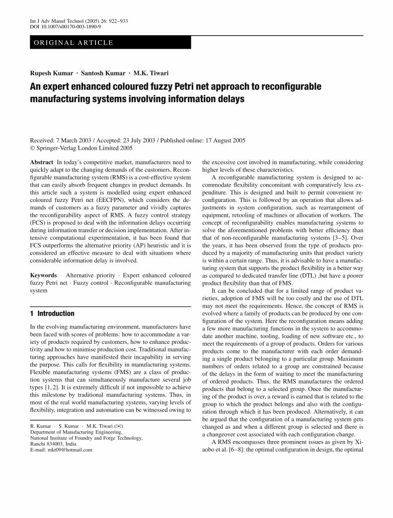
Fig. 1. Manufacturing system cost versus capacity (or production rate)(Adapted from Koren et al. [14])

The system cost vs. capacity graph for FMS and RMS isshown in Fig. 1, where the DMLs remain constant at its max-imum capacity and increase as and when the maximum capacityis increased. Also, the graph for FMS is scalable at a constantrate, i.e. as the machines are added in parallel. On the other hand,a RMS is scalable at a non-constant rate. The rate depends onthe design and market conditions. Table 1 shows a comparisonamong different types of manufacturing systems.

3 Formulation of the problem

The problem described in this paper is related to the machinereconfigurability. Here, each machine simultaneously producestwo parts. Each part is allocated to a dedicated input queue. Theprocessing operation selects a queue from which the next partshould be manufactured, i.e. the sequencing decision is queueselection decision (QSD) and it observes queue selection rule(QSR) as a sequencing rule.

3.1 Main characteristics of the proposed RMS

The main characteristics of the proposed RMS are as follows:

1. The system comprises of a single reconfigurable machineprocessing exactly two part types.

2. The two queues are supposed to be disjoint.3. Arrival rate of the two parts follow Poison distribution.4. Processing times of parts are distributed exponentially with

pre-specified mean parameters.5. Parts leave the system if and only if the processing is com-

pleted on the machines.6. QSD is affected by the control strategy applied which in turn

is affected by QSR.7. System performance is assessed within a pre-determined

time frame.8. Intentionally, a machine is never kept idle.

In order to apply the proposed selection criterion, an example isconsidered where o and o′ are the two orders arriving to the RMSat the same time. Let O be the set of orders and G is the set ofproduction objectives, each objective Gi is associated with a realvalued measurement scale si(o), where

si(o) = {o ∈ O, Gi ∈ G|sGi(o) ∈ Ri ⊆ R(i = 1, 2, 3. . . j)}.Let Df be the decision function that decides which job will beassigned first to a machine. For better makespan, the decisionfunction is designed to maximise the manufacturer’s evaluationfunction E f , which itself is a function of the manufacturer’s pref-erence ni . E f also depends on the real valued measurement scalesi(o) on the real line, R.

si(o) ∈ Ri (1)

si(o) ∈ si(O) (2)

si(o)∩ si(o′) = Φ (3)

Df (o) = maxo∈O

{E f (niψsi(o))}, i = {1, 2, 3. . . j}, (4)

925

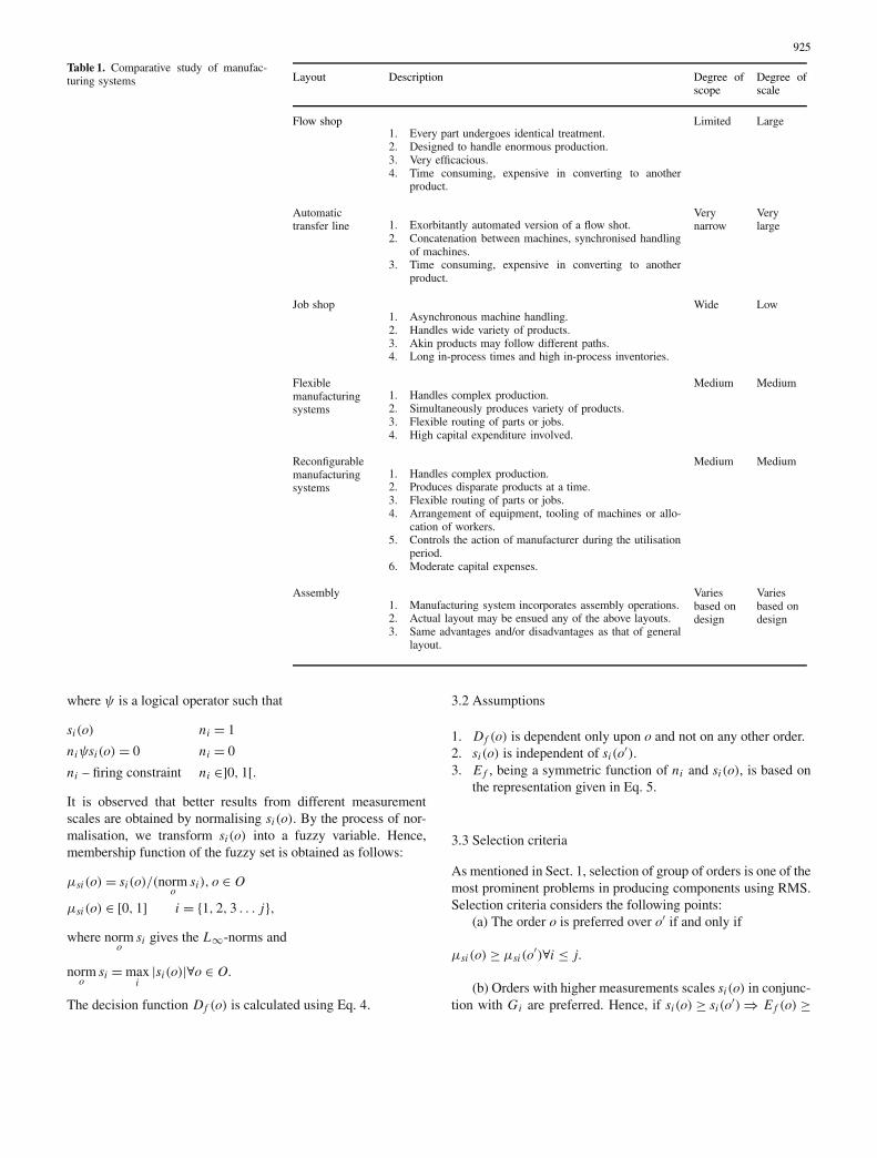
Layout Description Degree ofscope

Degree ofscale

Flow shop1. Every part undergoes identical treatment.2. Designed to handle enormous production.3. Very efficacious.4. Time consuming, expensive in converting to another

product.

Limited Large

Automatictransfer line 1. Exorbitantly automated version of a flow shot.

2. Concatenation between machines, synchronised handlingof machines.

3. Time consuming, expensive in converting to anotherproduct.

Verynarrow

Verylarge

Job shop1. Asynchronous machine handling.2. Handles wide variety of products.3. Akin products may follow different paths.4. Long in-process times and high in-process inventories.

Wide Low

Flexiblemanufacturingsystems

1. Handles complex production.2. Simultaneously produces variety of products.3. Flexible routing of parts or jobs.4. High capital expenditure involved.

Medium Medium

Reconfigurablemanufacturingsystems

1. Handles complex production.2. Produces disparate products at a time.3. Flexible routing of parts or jobs.4. Arrangement of equipment, tooling of machines or allo-

cation of workers.5. Controls the action of manufacturer during the utilisation

period.6. Moderate capital expenses.

Medium Medium

Assembly1. Manufacturing system incorporates assembly operations.2. Actual layout may be ensued any of the above layouts.3. Same advantages and/or disadvantages as that of general

layout.

Variesbased ondesign

Variesbased ondesign

Table 1. Comparative study of manufac-turing systems

where ψ is a logical operator such that

si(o) ni = 1

niψsi(o) = 0 ni = 0

ni – firing constraint ni ∈]0, 1[.It is observed that better results from different measurementscales are obtained by normalising si(o). By the process of nor-malisation, we transform si(o) into a fuzzy variable. Hence,membership function of the fuzzy set is obtained as follows:

µsi(o) = si(o)/(normo

si), o ∈ O

µsi(o) ∈ [0, 1] i = {1, 2, 3 . . . j},where norm

osi gives the L∞-norms and

normo

si = maxi

|si(o)|∀o ∈ O.

The decision function Df (o) is calculated using Eq. 4.

3.2 Assumptions

1. Df (o) is dependent only upon o and not on any other order.2. si(o) is independent of si(o′).3. E f , being a symmetric function of ni and si(o), is based on

the representation given in Eq. 5.

3.3 Selection criteria

As mentioned in Sect. 1, selection of group of orders is one of themost prominent problems in producing components using RMS.Selection criteria considers the following points:

(a) The order o is preferred over o′ if and only if

µsi(o) ≥ µsi(o′)∀i ≤ j.

(b) Orders with higher measurements scales si(o) in conjunc-tion with Gi are preferred. Hence, if si(o) ≥ si(o′) ⇒ E f (o) ≥

926

E f (o′)∀i ≤ j . These two objectives are obtained simultaneouslyby allowing a trade-off for the evaluation of the measurementscales such that the selection order lies between the worst and thebest individual orders.

(c) For any two goals Gi and G ′i of equal importance, i.e.

having similar membership functions µ1 and µ2, an averagingoperator is chosen for aggregations,

E f (µ1, µ2) = (µ1 +µ2)/2.

For any symmetric summation, E f can be represented as:

E f (µ1, µ2, . . .µn) = z(µ1, µ2, . . .µn)

z(µ1, µ2, . . .µn)+ z(1−µ1, 1−µ2, . . .1−µn), (5)

where z(µ1, µ2, . . . µn) is a non-negative, commutative, contin-uous, real mapping. Hence, to select z(µ1, µ2, . . . µn) valuessuch that

z(µ1, µ2, . . .µn) = µ1 +µ2 + . . .µn|z(0, 0, 0, . . ..0) = 0.

Hence,

E f (µ1, µ2, . . .µn) = (µ1 +µ2 + . . .µn)/n

= (Σµn)/n.

The E f is calculated for both the orders and the manufacturerselects the one having higher value.

4 Expert enhanced coloured fuzzy Petri net (EECFPN)

In order to get a better view of the working of the reconfigurablemanufacturing system, it is modelled using EECFPN. Followingare a few definitions that are needed to comprehend the mod-elling capability of EECFPN.

4.1 Definition

The EECFPN is an extension of Petri nets and it is used in thisarticle to model a system having some fuzzy truth values as-signed to various rules affecting the modelling behaviour. TheEECFPN is defined as a septuple:

EECFPN ≡ {P, T, A, W, M, C, R},where(i) P is a set of places satisfying the relation

P = PN ∪ PI ∪ PC ∪ PT ,

where PN is the set of normal places, PI is the set of inhibitorplaces, PC is the set of control places, PT is the set of transitionplaces, PN ∩ PI = φ, PC ∩ PT = φ, PI ∩ PT = φ, PN ∩ PC = φ,PN ∩ PT = φ, and PI ∩ PC = φ. PN ∪ PI �= φ, PC ∪ PT �= φ, PI ∪PT �= φ, PN ∪ PC �= φ, PN ∪ PT �= φ, and PI ∪ PC �= φ.

Normal place (PN): It depicts the feasible parts involved inthe manufacturing process:

PN = {p1, p2, p3, . . . }.

Inhibitor place (PI): It shows the components involvedin manufacturing processes that are not desirable but are stillproduced:

PI = {pi1, pi2, pi3, . . . }.

Control place (PC): These are places associated with flow-control of the manufacturing process. Control place finds itsapplication when there is more than one feasible plan. It selectsthe optimal plan amongst the various feasible plans:

PC = {pC1, pC2, pC3 . . . }.

Transition place (PT ): These are places associated withtransitions having at least one incoming arc. Their function is toavoid refraction (phenomenon of uncontrolled looping betweena transition and a place). The arcs associated with transitionplaces are always directed from transition place to the respectivetransition:

PT = {pT 1, pT 2, pT 3 . . . }.

(ii) T is a set of transitions, such that

T = {t1, t2, t3 . . . }.

(iii) A is a set of arcs, such that

A = I ∪ O

I ∩ O = φ, I ∪ O �= φ, where I is a set of input arcs

and O is a set of output arcs,

I = Ie ∪ II and O = Oe ∪ OI .

Ie is a set of excitant input arcs, and Ii is a set of inhibitorinput arcs:

Ie ∪ Ii �= φ and Ie ∩ Ii = φ.

Oe is a set of excitant output arcs, and OI is a set of inhibitoroutput arcs:

Oe ∪ Oi �= φ and Oe ∩ Oi = φ.

Excitant arcs: These are the arcs connecting places and tran-sitions, where feasible operations take place:

Ae = Ie ∪ Oe

Ie ∪ Oe �= φ and Ie ∩ Oe = φ,

where Ae is the set of excitant arcs.

927

Inhibitor arcs: These are the arcs connecting places andtransitions, where operations taking place are not fruitful:

Ai = Ii ∪ Oi

Ii ∪ Oi �= φ, Ii ∩ Oi = φ,

where Ai is the set of inhibitor arcs.Arc set A can also be classified on the basis of tokens present

in the place linked with the arc:

A = Ag ∪ Ar,

where Ag is a set of arcs associated with places containing greentokens, and Ar is a set of arcs associated with places containingred tokens.(iv) W is a set of weight of the arcs. It is mentioned with the helpof the numbers shown with the arc. In case it is not mentioned, itsvalue is taken as unity.(v) M is a set of marking:

M : P → {0, 1, 2. . .}M = {NT (p1), NT (p2), . . .}and M = Mg ∪ Mr,

where Mg is the marking of places containing green tokens, andMr is the marking of places containing red tokens. A, mx1 ma-trix represents marking M for a set of m places.

State equation: Let Mk be the marking after the kth firing,Mk−1 be the marking after the (k −1)th firing, A be the incidencematrix denoting the change of marking. Then, Mk = Mk−1 +AT Uk, ∀k = 1, 2, 3 . . . , where Uk is a nx1 column matrix, and isknown as a “control vector”. It consists of (n −1) 0’s and a 1 inthe tth position. 1 indicates that transition “t” fire at the kth firing.

Reachibility condition: If Mk is a reachable marking fromM0, through a firing sequence {u1, u2, u3, . . . }, then the condi-tion for reachability is

Mk = M0 + ATk∑

k=1

uk

⇒ Mk − M0 = ATk∑

k=1

uk

∆M = Mk − M0 ≡ change in marking

∆M = ATk∑

k=1

uk.

(vi) C is a set of colours associated with tokens:

C = {g, r},

where “g” stands for green colour, and “r” stands for red colour.Green tokens are associated with occurrence of positive

events. Here, the associated arcs belong to the set of excitantarcs.

Red colour shows the nth occurrence of negative events, i.e.non-occurrence of fruitful events. Here the associated arcs be-long to the set of inhibitor arcs. Red tokens are further classifiedinto two groups, i.e. default red and deduced red. Default redmarking indicates that the occurrence of an event is assumedto be false under close-world assumption (CWA), while the de-duced red indicates that the occurrence of event is proved to befalse.

A transition t ∈ T is enabled under marking M = Mg ∪ Mr

iff,

colour (Lg(p, t)) ∈ Mg(p), ∀p ∈ I, (p, t) ∈ Ag

colour (Lr (p, t)) ∈ Mr(p), ∀p ∈ I, (p, t) ∈ Ar .

After firing of a transition, tokens leave the input places re-sulting in a change in the marking state. Suppose transition t firesunder initial marking Mg. It loses green tokens represented bythe term “colour (Lg(p, t))”.

At the same time, if there is an arc from t to p, some greentokens get added. This is given by the term “colour (Lg(t, p))”.

The new marking M′g(p) is given by

M′g(p) = Mg(p) – colour (Lg(p, t))+ colour (Lg(t, p)), (6)

and

M′r(p) = Mr(p) – Colour (Lr(p, t))+Colour (Lr(t, p)). (7)

(vii) R is a set of fuzzy truth values associated with various tran-sitions. In order to further elucidate the idea behind the needof the EECFPN, the advantages of expert enhanced colouredstochastic Petri net (EECSPN) over normal Petri net (NPN) andexpert Petri net (EPN) are discussed in the Table 2.

4.2 Colouring of the EECFPN model

In order to delineate the procedures that are inherently embed-ded in the EECFPN, the steps involved in the colouring are givenbelow:

1. Initially, every transition place is assigned a green colouredtoken.

2. Every control place, as they are associated with positiveevents, are initially assigned a green token.

3. Every place other than transition place is assigned a defaultred token.

4. With every positive event, a green token is assigned.5. With every negative event that is proved to be false, a de-

duced red token is assigned.6. With every negative event which is assumed to be false, a de-

fault red token is assigned.7. Firing of a transition results in the transfer of tokens from the

incoming place to the outgoing place.8. When an event is proved to be false, which was initially as-

sumed to be false, the token inhibitor place associated withthe event loses a default red token and gains a deduced redtoken.

928

Properties Normal Petri net Expert Petri net Expert enhanced(NPN) (EPN) coloured stochastic

Petri net (EECSPN)Firing of transition Transition enabled An enabled An enabled

as soon as input transition will fire transition fires onlyplaces have tokens when events when rules

associated with the associated with ittransition occur are satisfied

Control over firing No control Control by means Control by meansof control places of control places

Time as a parameter Not considered Considered in terms Considered in termsof timed transitions of timed transitions

Goal places Not defined Defined DefinedProbability of occurrence Not considered Not considered ConsideredColour identification Not considered Not considered ConsideredRule-based labels Not considered Not considered ConsideredRefraction prevention Not considered Not considered ConsideredConsideration of Not considered Not considered Considerednegative events

Table 2. Comparison of normal Petri net(NPN), expert Petri net (EPN) and expertenhanced coloured stochastic Petri net (EEC-SPN)

Let M0 be the initial marking, M0g the initial green marking,

M0dd the initial deduced red marking, and M0

d f the initial defaultred marking.

Clearly,

1. M0g(pTi) = C(ti )

2. M0dd(pTi ) = M0

d f (pTi ) = φ, ∀pTi ∈ PT

3. M0g(p) = M0

dd(p) = φ

4. M0d f (p) = C(p), ∀p ∈ P − PT .

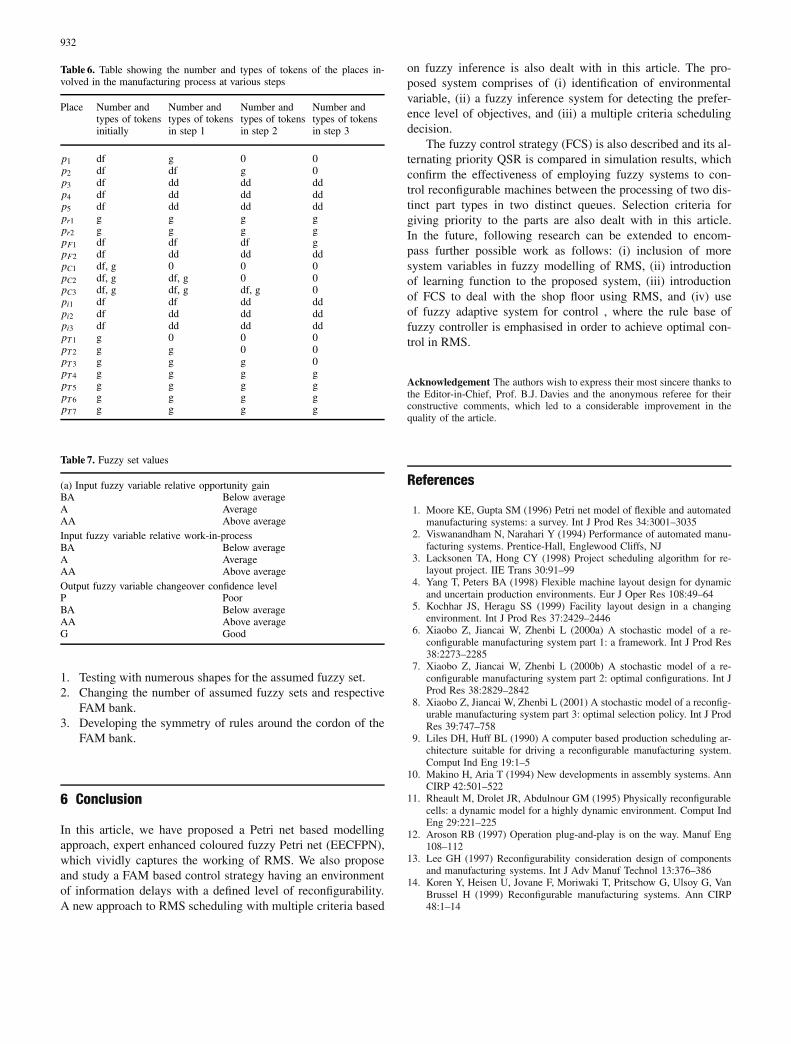
Table 3 shows the marking and colouring of the EECFPNmodel for the two job types at various steps.

Table 3. Designation of places involved in the manufacturing process asshown in Figs. 3, 4, 5 and 6, respectively

Places Designation

p1 Incoming place for first job typep2 Intermediate place after first transition for first job typep3 Incoming place for second job typep4 Intermediate place after first transition for second job typep5 Intermediate place after second transition for second job typepr1 Resource place for first transition of both the job typespr2 Resource place for second transition of both the job typespC1 Control place for the preference of job typespC2 Control place for first transition of both the job typespC3 Control place for second transition of both the job typespF1 Output place for first job typepF2 Output place for second job typepi1 Inhibitor place for first job type after its first transitionpi2 Inhibitor place for first job type after its second transitionpi3 Inhibitor place for second job type after its first transitionpT1 Transition place for selection of first job typepT2 Transition place for first job type after its first transitionpT3 Transition place for first job type after its second transitionpT4 Transition place for selection of second job typepT5 Transition place for second job type after its first transitionpT6 Transition place for second job type after its second transitionpT7 Transition place for second job type after its third transition

Change of marking: When a transition fires, the marking ofthe network gets changed. For instance, let a transition “t” have“m” negative inplaces, some of them being enabled by defaultred colours and the rest by deduced red colours. When t fires, themarking M changes to marking M′.

Clearly,

1.

M′ = M′g ∩ (M′

dd ∩ M′d f )

2.

M′g(p) = Mg(p)− colour (Lg(p, t))+ colour (Lg(t, p))

3.

M′dd(p) = Mdd(p)− colour (Lr(p, t))+ colour (L ′

r (p, t))

+ colour (Lr(t, p)) (8)

4.

M′d f (p) = Md f (p)− colour (Lr (p, t))− colour (Lg(p, t))

+ colour (L ′r (t, p))− colour (L ′

g(t, p))

− colour (Lg(p, t)).

It is worthwhile to note that colour (Lr(p, t)) signifiesthose red colours flowing through the input arcs and the colour(L ′

r(p, t)) denotes the feedback red colours corresponding tothese. Similarly, M′

d f (p, t), colour (Lr(p, t)) signifies those de-fault red colours which had flown through the input arcs andcolour (L ′r(t, p)) denotes the feedback red colours correspond-ing to these.

Therefore

colour (Lr (p, t)) =colour (L ′r(p, t))

for both M′dd(p) and M′

d f (p),

929

where

colour (Lg(p, t)) ⊆ colour (Lg(t, p)).

Hence, the equations mentioned above can be simplified to:

M′g(p) = Mg(p)− colour (Lg(p, t))+ colour (Lg(t, p))

M′dd(p) = Mdd(p)+ colour (Lr(t, p))

M′d f (p) = Md f (p)− colour (Lg(t, p))− colour (Lr(t, p)) (9)

Md f (p)∩ Mdd(p) = φ and Md f (p)∩ Mg(p) = φ.

Any intermediate marking, and hence, any intermediate stageinvolved in the operation can be found out by using the afore-mentioned equations.

4.3 Comparison of EECFPN model with classical Petri netmodel

Here, considering an example of two-part types with differentprocessing Requirements, a comparison is established for thetwo models.

EECFPNs provide a powerful means to specify the systemperformance. EECFPNs are efficacious in determining optimalconfiguration and carry out structural and analytical performanceanalysis. On the other hand, classical PNs are unable to performzero testing [16–18]. This limitation is evinced by the accretionof inhibitor arcs.

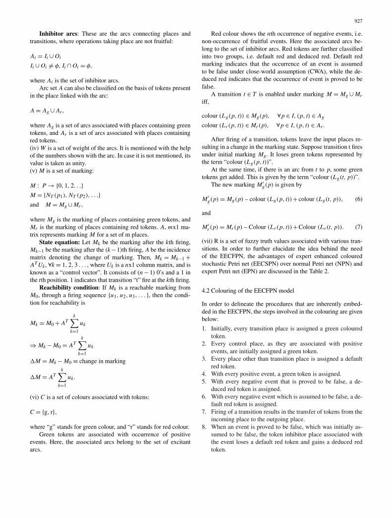
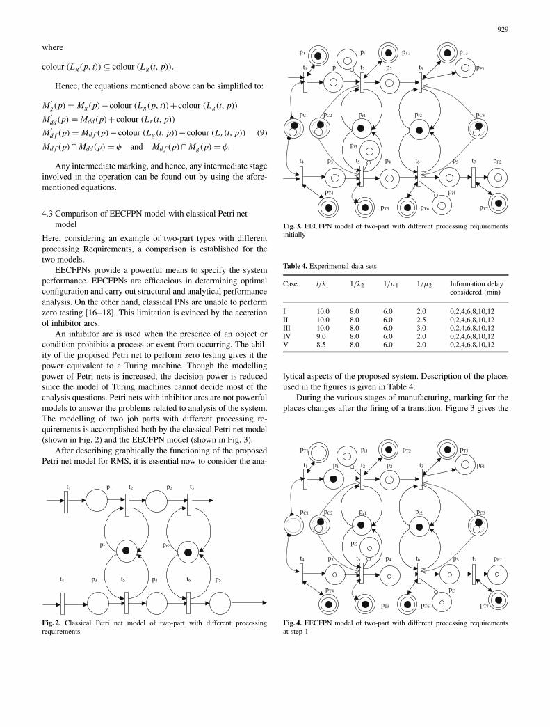
An inhibitor arc is used when the presence of an object orcondition prohibits a process or event from occurring. The abil-ity of the proposed Petri net to perform zero testing gives it thepower equivalent to a Turing machine. Though the modellingpower of Petri nets is increased, the decision power is reducedsince the model of Turing machines cannot decide most of theanalysis questions. Petri nets with inhibitor arcs are not powerfulmodels to answer the problems related to analysis of the system.The modelling of two job parts with different processing re-quirements is accomplished both by the classical Petri net model(shown in Fig. 2) and the EECFPN model (shown in Fig. 3).

After describing graphically the functioning of the proposedPetri net model for RMS, it is essential now to consider the ana-

Fig. 2. Classical Petri net model of two-part with different processingrequirements

Fig. 3. EECFPN model of two-part with different processing requirementsinitially

Table 4. Experimental data sets

Case l/λ1 1/λ2 1/µ1 1/µ2 Information delayconsidered (min)

I 10.0 8.0 6.0 2.0 0,2,4,6,8,10,12II 10.0 8.0 6.0 2.5 0,2,4,6,8,10,12III 10.0 8.0 6.0 3.0 0,2,4,6,8,10,12IV 9.0 8.0 6.0 2.0 0,2,4,6,8,10,12V 8.5 8.0 6.0 2.0 0,2,4,6,8,10,12

lytical aspects of the proposed system. Description of the placesused in the figures is given in Table 4.

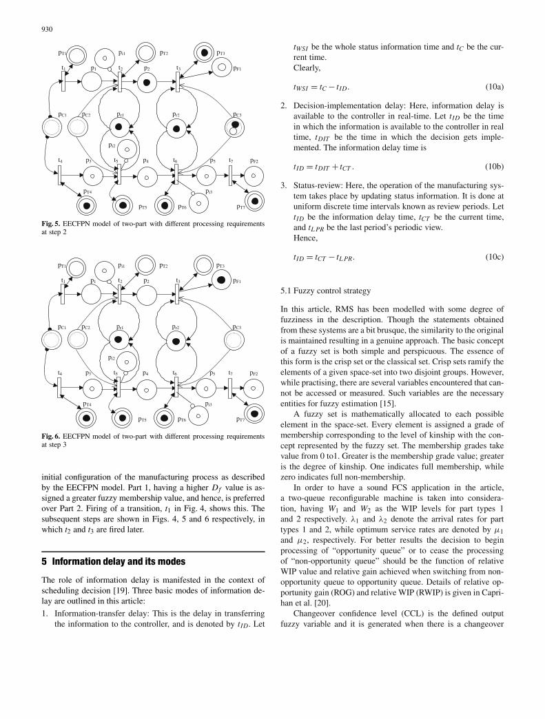
During the various stages of manufacturing, marking for theplaces changes after the firing of a transition. Figure 3 gives the

Fig. 4. EECFPN model of two-part with different processing requirementsat step 1

930

Fig. 5. EECFPN model of two-part with different processing requirementsat step 2

Fig. 6. EECFPN model of two-part with different processing requirementsat step 3

initial configuration of the manufacturing process as describedby the EECFPN model. Part 1, having a higher Df value is as-signed a greater fuzzy membership value, and hence, is preferredover Part 2. Firing of a transition, t1 in Fig. 4, shows this. Thesubsequent steps are shown in Figs. 4, 5 and 6 respectively, inwhich t2 and t3 are fired later.

5 Information delay and its modes

The role of information delay is manifested in the context ofscheduling decision [19]. Three basic modes of information de-lay are outlined in this article:

1. Information-transfer delay: This is the delay in transferringthe information to the controller, and is denoted by tID. Let

tWSI be the whole status information time and tC be the cur-rent time.Clearly,

tWSI = tC − tID. (10a)

2. Decision-implementation delay: Here, information delay isavailable to the controller in real-time. Let tID be the timein which the information is available to the controller in realtime, tDIT be the time in which the decision gets imple-mented. The information delay time is

tID = tDIT + tCT . (10b)

3. Status-review: Here, the operation of the manufacturing sys-tem takes place by updating status information. It is done atuniform discrete time intervals known as review periods. LettID be the information delay time, tCT be the current time,and tL PR be the last period’s periodic view.Hence,

tID = tCT − tL PR. (10c)

5.1 Fuzzy control strategy

In this article, RMS has been modelled with some degree offuzziness in the description. Though the statements obtainedfrom these systems are a bit brusque, the similarity to the originalis maintained resulting in a genuine approach. The basic conceptof a fuzzy set is both simple and perspicuous. The essence ofthis form is the crisp set or the classical set. Crisp sets ramify theelements of a given space-set into two disjoint groups. However,while practising, there are several variables encountered that can-not be accessed or measured. Such variables are the necessaryentities for fuzzy estimation [15].

A fuzzy set is mathematically allocated to each possibleelement in the space-set. Every element is assigned a grade ofmembership corresponding to the level of kinship with the con-cept represented by the fuzzy set. The membership grades takevalue from 0 to1. Greater is the membership grade value; greateris the degree of kinship. One indicates full membership, whilezero indicates full non-membership.

In order to have a sound FCS application in the article,a two-queue reconfigurable machine is taken into considera-tion, having W1 and W2 as the WIP levels for part types 1and 2 respectively. λ1 and λ2 denote the arrival rates for parttypes 1 and 2, while optimum service rates are denoted by µ1and µ2, respectively. For better results the decision to beginprocessing of “opportunity queue” or to cease the processingof “non-opportunity queue” should be the function of relativeWIP value and relative gain achieved when switching from non-opportunity queue to opportunity queue. Details of relative op-portunity gain (ROG) and relative WIP (RWIP) is given in Capri-han et al. [20].

Changeover confidence level (CCL) is the defined outputfuzzy variable and it is generated when there is a changeover

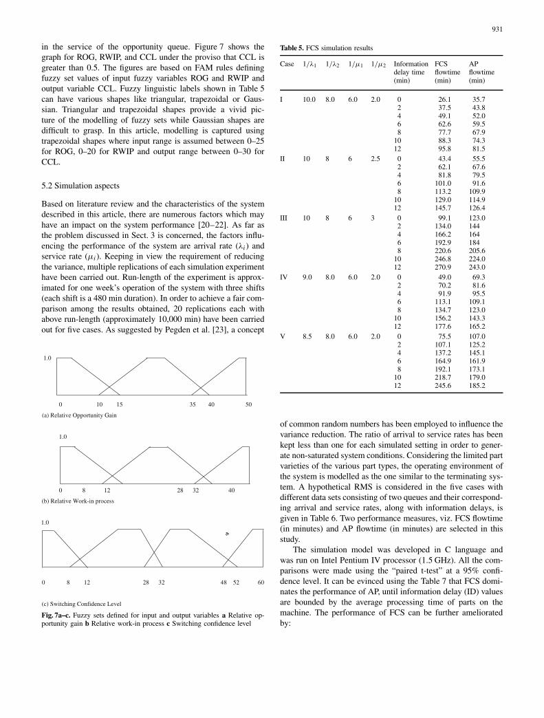
931

in the service of the opportunity queue. Figure 7 shows thegraph for ROG, RWIP, and CCL under the proviso that CCL isgreater than 0.5. The figures are based on FAM rules definingfuzzy set values of input fuzzy variables ROG and RWIP andoutput variable CCL. Fuzzy linguistic labels shown in Table 5can have various shapes like triangular, trapezoidal or Gaus-sian. Triangular and trapezoidal shapes provide a vivid pic-ture of the modelling of fuzzy sets while Gaussian shapes aredifficult to grasp. In this article, modelling is captured usingtrapezoidal shapes where input range is assumed between 0–25for ROG, 0–20 for RWIP and output range between 0–30 forCCL.

5.2 Simulation aspects

Based on literature review and the characteristics of the systemdescribed in this article, there are numerous factors which mayhave an impact on the system performance [20–22]. As far asthe problem discussed in Sect. 3 is concerned, the factors influ-encing the performance of the system are arrival rate (λi ) andservice rate (µi ). Keeping in view the requirement of reducingthe variance, multiple replications of each simulation experimenthave been carried out. Run-length of the experiment is approx-imated for one week’s operation of the system with three shifts(each shift is a 480 min duration). In order to achieve a fair com-parison among the results obtained, 20 replications each withabove run-length (approximately 10,000 min) have been carriedout for five cases. As suggested by Pegden et al. [23], a concept

Fig. 7a–c. Fuzzy sets defined for input and output variables a Relative op-portunity gain b Relative work-in process c Switching confidence level

Table 5. FCS simulation results

Case 1/λ1 1/λ2 1/µ1 1/µ2 Information FCS APdelay time flowtime flowtime(min) (min) (min)

I 10.0 8.0 6.0 2.0 0 26.1 35.72 37.5 43.84 49.1 52.06 62.6 59.58 77.7 67.9

10 88.3 74.312 95.8 81.5

II 10 8 6 2.5 0 43.4 55.52 62.1 67.64 81.8 79.56 101.0 91.68 113.2 109.9

10 129.0 114.912 145.7 126.4

III 10 8 6 3 0 99.1 123.02 134.0 1444 166.2 1646 192.9 1848 220.6 205.6

10 246.8 224.012 270.9 243.0

IV 9.0 8.0 6.0 2.0 0 49.0 69.32 70.2 81.64 91.9 95.56 113.1 109.18 134.7 123.0

10 156.2 143.312 177.6 165.2

V 8.5 8.0 6.0 2.0 0 75.5 107.02 107.1 125.24 137.2 145.16 164.9 161.98 192.1 173.1

10 218.7 179.012 245.6 185.2

of common random numbers has been employed to influence thevariance reduction. The ratio of arrival to service rates has beenkept less than one for each simulated setting in order to gener-ate non-saturated system conditions. Considering the limited partvarieties of the various part types, the operating environment ofthe system is modelled as the one similar to the terminating sys-tem. A hypothetical RMS is considered in the five cases withdifferent data sets consisting of two queues and their correspond-ing arrival and service rates, along with information delays, isgiven in Table 6. Two performance measures, viz. FCS flowtime(in minutes) and AP flowtime (in minutes) are selected in thisstudy.

The simulation model was developed in C language andwas run on Intel Pentium IV processor (1.5 GHz). All the com-parisons were made using the “paired t-test” at a 95% confi-dence level. It can be evinced using the Table 7 that FCS domi-nates the performance of AP, until information delay (ID) valuesare bounded by the average processing time of parts on themachine. The performance of FCS can be further amelioratedby:

932

Table 6. Table showing the number and types of tokens of the places in-volved in the manufacturing process at various steps

Place Number and Number and Number and Number andtypes of tokens types of tokens types of tokens types of tokensinitially in step 1 in step 2 in step 3

p1 df g 0 0p2 df df g 0p3 df dd dd ddp4 df dd dd ddp5 df dd dd ddpr1 g g g gpr2 g g g gpF1 df df df gpF2 df dd dd ddpC1 df, g 0 0 0pC2 df, g df, g 0 0pC3 df, g df, g df, g 0pi1 df df dd ddpi2 df dd dd ddpi3 df dd dd ddpT1 g 0 0 0pT2 g g 0 0pT3 g g g 0pT4 g g g gpT5 g g g gpT6 g g g gpT7 g g g g

Table 7. Fuzzy set values

(a) Input fuzzy variable relative opportunity gainBA Below averageA AverageAA Above averageInput fuzzy variable relative work-in-processBA Below averageA AverageAA Above averageOutput fuzzy variable changeover confidence levelP PoorBA Below averageAA Above averageG Good

1. Testing with numerous shapes for the assumed fuzzy set.2. Changing the number of assumed fuzzy sets and respective

FAM bank.3. Developing the symmetry of rules around the cordon of the

FAM bank.

6 Conclusion

In this article, we have proposed a Petri net based modellingapproach, expert enhanced coloured fuzzy Petri net (EECFPN),which vividly captures the working of RMS. We also proposeand study a FAM based control strategy having an environmentof information delays with a defined level of reconfigurability.A new approach to RMS scheduling with multiple criteria based

on fuzzy inference is also dealt with in this article. The pro-posed system comprises of (i) identification of environmentalvariable, (ii) a fuzzy inference system for detecting the prefer-ence level of objectives, and (iii) a multiple criteria schedulingdecision.

The fuzzy control strategy (FCS) is also described and its al-ternating priority QSR is compared in simulation results, whichconfirm the effectiveness of employing fuzzy systems to con-trol reconfigurable machines between the processing of two dis-tinct part types in two distinct queues. Selection criteria forgiving priority to the parts are also dealt with in this article.In the future, following research can be extended to encom-pass further possible work as follows: (i) inclusion of moresystem variables in fuzzy modelling of RMS, (ii) introductionof learning function to the proposed system, (iii) introductionof FCS to deal with the shop floor using RMS, and (iv) useof fuzzy adaptive system for control , where the rule base offuzzy controller is emphasised in order to achieve optimal con-trol in RMS.

Acknowledgement The authors wish to express their most sincere thanks tothe Editor-in-Chief, Prof. B.J. Davies and the anonymous referee for theirconstructive comments, which led to a considerable improvement in thequality of the article.

References

1. Moore KE, Gupta SM (1996) Petri net model of flexible and automatedmanufacturing systems: a survey. Int J Prod Res 34:3001–3035

2. Viswanandham N, Narahari Y (1994) Performance of automated manu-facturing systems. Prentice-Hall, Englewood Cliffs, NJ

3. Lacksonen TA, Hong CY (1998) Project scheduling algorithm for re-layout project. IIE Trans 30:91–99

4. Yang T, Peters BA (1998) Flexible machine layout design for dynamicand uncertain production environments. Eur J Oper Res 108:49–64

5. Kochhar JS, Heragu SS (1999) Facility layout design in a changingenvironment. Int J Prod Res 37:2429–2446

6. Xiaobo Z, Jiancai W, Zhenbi L (2000a) A stochastic model of a re-configurable manufacturing system part 1: a framework. Int J Prod Res38:2273–2285

7. Xiaobo Z, Jiancai W, Zhenbi L (2000b) A stochastic model of a re-configurable manufacturing system part 2: optimal configurations. Int JProd Res 38:2829–2842

8. Xiaobo Z, Jiancai W, Zhenbi L (2001) A stochastic model of a reconfig-urable manufacturing system part 3: optimal selection policy. Int J ProdRes 39:747–758

9. Liles DH, Huff BL (1990) A computer based production scheduling ar-chitecture suitable for driving a reconfigurable manufacturing system.Comput Ind Eng 19:1–5

10. Makino H, Aria T (1994) New developments in assembly systems. AnnCIRP 42:501–522

11. Rheault M, Drolet JR, Abdulnour GM (1995) Physically reconfigurablecells: a dynamic model for a highly dynamic environment. Comput IndEng 29:221–225

12. Aroson RB (1997) Operation plug-and-play is on the way. Manuf Eng108–112

13. Lee GH (1997) Reconfigurability consideration design of componentsand manufacturing systems. Int J Adv Manuf Technol 13:376–386

14. Koren Y, Heisen U, Jovane F, Moriwaki T, Pritschow G, Ulsoy G, VanBrussel H (1999) Reconfigurable manufacturing systems. Ann CIRP48:1–14

933

15. Kosko B (1992) Neural networks and fuzzy systems: a dynamicalsystems approach to machine intelligence. Prentice-Hall, EnglewoodCliffs, NJ

16. Patil S (1971) Limitation and capabilities of Dijksta’s semaphore primi-tives for coordination among processes. MIT project MAC computationStructure Group Memo 57, MIT, Cambridge, MA

17. Agerwala T, Flynn M (1973) Comments on capabilities, limitations andcorrectness of Petri nets. Proceedings of the 1st Annual Symposium onComputer Architectures ACM, pp 81–86

18. Peterson JL (1981) Petri net theory and the modelling of systems.Prentice-Hall, Englewood Cliffs, NJ

19. Conway RW, Maxwell WL, Miller LW (1967) Theory of scheduling.Addison-Wesley, Reading, MA

20. Caprihan R, Kumar S, Wadhwa S (1997) Fuzzy systems for control offlexible machines operating under information delays. Int J Prod Res5:1331–1348

21. Yu L, Shih HM, Sekiguchi T (1999) Fuzzy inference-based multiplecriteria FMS scheduling. Int J Prod Res 37:2315–2333

22. Desrochers AA (1990) Modelling and control of automated manufac-turing systems. IEEE Computer Society, Washington, DC

23. Pegden CD, Shanon RP, Sadowski RP (1990) Introduction to simulationusing SIMIAN. McGraw-Hill, New York