An evaluation of the estimation of road traffic emission factors from tracer studies

lable at ScienceDirect

Atmospheric Environment 44 (2010) 3814e3822

Contents lists avai

Atmospheric Environment

journal homepage: www.elsevier .com/locate/atmosenv

An evaluation of the estimation of road traffic emission factors from tracer studies

Luis Carlos Belalcazar a,*, Alain Clappier b,c, Nadège Blond b,c, Thomas Flassak d, Joachim Eichhorn e

aAir and Soil Pollution Laboratory (LPAS), Swiss Federal Institute of Technology (EPFL), Station 2, 1015-Lausanne, SwitzerlandbUniversité de Strasbourg, Laboratoire Image Ville Environnement, F-67000 Strasbourg, FrancecCNRS, Laboratoire Image Ville Environnement, F-67000 Strasbourg, Franced Ingenieurbuero Lohmeyer GmbH & Co. KG, D-76229 Karlsruhe, Germanye Theoretical Meteorology Group, Institute for Atmospheric Physics, University of Mainz, Germany

a r t i c l e i n f o

Article history:Received 10 February 2010Received in revised form18 June 2010Accepted 21 June 2010

Keywords:Street canyonComputational Fluids Dynamics (CFD)Tracer studiesModel validationReal-world motor vehicle emissions

* Corresponding author. Tel.: þ41 21 693 57 01; faxE-mail address: [email protected] (L.C. Be

1352-2310/$ e see front matter � 2010 Elsevier Ltd.doi:10.1016/j.atmosenv.2010.06.038

a b s t r a c t

Road traffic emission factors (EFs) are one of the main sources of uncertainties in emission inventories; itis necessary to develop methods to reduce these uncertainties to manage air quality more efficiently.Recently an alternative method has been proposed to estimate the EFs. In that work the emission factorswere estimated from a long term tracer study developed in Ho Chi Minh City (HCMC) Vietnam. A passivetracer was continuously emitted from a finite line source placed in one side of an urban street canyon.Simultaneously, the resulting tracer concentrations were monitored at the other side of the street. Theresults of this experiment were used to calculate the dispersion factors and afterwards, these dispersionfactors were used to estimate the EFs. In this paper we use the Computational Fluids Dynamics (CFD)model WinMISKAM to critically evaluate the proposed methodology.

In a first step, we use the results of the tracer study to validate the CFD model. Results show that themodel is able to simulate quite well the tracer dispersion in most of the cases. The model is then used toevaluate the effect of varying the source configuration and to correct the EFs. A comparison with availablestudies shows that the corrected EFs are within the range of the EFs reported in other studies. Finally, theCFD model is used to find a source configuration that better represents the vehicle emissions and thatmay be used in future studies to estimate the EFs more accurately. Results show that a 200 m line placedin the center of the street would represent very well the vehicle emissions. This work shows that it ispossible to accurately estimate the EFs from tracer studies.

� 2010 Elsevier Ltd. All rights reserved.

1. Introduction

Road traffic emission factors (EFs) are one of the main sources ofuncertainties in emission inventories; it is necessary to reducethese uncertainties to manage air quality more efficiently (Molinaand Molina, 2004). Two different approaches have been devel-oped to estimate vehicle EFs in a city, these approaches are knownas bottom-up and top-down. The most representative bottom-uptechniques are chassis dynamometer and on board emissionsmeasurements. The most used top-down techniques are tunnelstudies and inverse modeling.

Top-down techniques have been developed to overcome thelimitations of the bottom-up techniques; however, existing top-down methods also face limitations and uncertainties.

Inverse modeling has been used to estimate the EFs in differentcities of the world (Palmgren et al., 1999: Gramotnev et al., 2002;

: þ41 21 693 36 26.lalcazar).

All rights reserved.

Ketzel et al., 2003; Kawashima et al., 2006; Zárate et al., 2007).The main advantage of this technique is that it is possible tocalculate the EFs under real urban conditions. On the other hand, itsmain limitation is that the accuracy of the calculations depends onthe ability of the models to accurately reproduce the dispersion ofthe pollutants.

The inverse modeling technique uses a microscale operationalmodel or a Computational Fluids Dynamic (CFD) model to computethe dispersion. Operational models are based on a number ofempirical assumptions and parameters that cannot be applicable toall urban environments (Vardoulakis et al., 2003). While CFDmodels are designed to be used in any urban configuration, most ofthe research conducted to date used theoretical building configu-rations or measurements collected in reduced scale laboratoryexperiments to evaluate these models (Li et al., 2006; Benson et al.,2008; Donnelly et al., 2009). In addition, an important limitation ofCFD model validation in real urban conditions has been theuncertainties in the input information such as the vehicle emissionfactors (Lohmeyer et al., 2002; Vardoulakis et al., 2003; Gidhagenet al., 2004; Dixon et al., 2006; Holmes and Morawska, 2006).

L.C. Belalcazar et al. / Atmospheric Environment 44 (2010) 3814e3822 3815

CFD models also face uncertainties associated to the boundaryconditions, to the turbulence closure used and to the difficultiesassociated to the simulations of complex processes such as thermaleffects and traffic induced turbulence (Li et al., 2006).

Recently an alternative method has been proposed to estimatethe EFs (Belalcazar et al., 2009). In that work the EFs were estimatedfrom a long term tracer study carried out in Ho Chi Minh City(HCMC) Vietnam. In the HCMC tracer experiment, a passive tracersubstance (propane) was continuously emitted from a finite linesource placed in one side of an urban street canyon. Simulta-neously, the resulting tracer concentrations were monitored on-line at the other side of the street. The results of this experimentwere used to calculate the dispersion factors and afterwards, thesedispersion factors were used together with traffic counts androadside pollutant measurements to estimate the EFs. Theproposed method assumes that a finite emission line placed in oneside of the street represents the emissions produced by road traffic.However, traffic emissions are released in the whole area of thestreet, and thus there is an error associated to this assumption.

In this paper, we use the CFD model WinMISKAM to estimatethe error associated with the source position in HCMC and tocorrect the estimated EFs. In a first phase, we use the results of thetracer experiment to validate the CFDmodel. Here the CFDmodel isvalidated using a long term tracer study conducted in real urbanconditions. Moreover, the uncertainty associated with the emis-sions is reduced from the evaluation process because the traceremission rate is known.

Subsequently, the CFD model is used to calculate the dispersionfactors when the tracer is emitted from the line source (in the sameway the tracer was emitted during theHCMC tracer study) and fromthe full length and width of the street (in the same way the trafficemissions are produced). The results of these simulations areused tocompute the error produced by the source position in HCMC and tocorrect the EFs. In a last phase, the CFDmodel is used to evaluate theimpact of different source positions and lengths on the accuracy ofthe calculated vehicle emission factors from tracer studies. The

Fig. 1. Left: (a) satellite Image of the Ba Thang Hai street. 1: emission line; 2: Monitoring sGoogle Earth, downloaded in May 2009). Right: (b) WinMISKAM computational domain, thepoint are also indicated in the center of figure (b).

results of these simulations are used tofind the source configurationthat better approximates the road traffic emission and that may beused in future tracer studies to calculate the EFs more accurately.

2. Methodology

2.1. The Ho Chi Minh City (HCMC) tracer study

In this work we use the results of a long term tracer experimentwhich was conducted from January to March 2007 in the Ba ThangHai (BTH) street, close to the center of HCMC (Belalcazar et al.,2009). The tracer was emitted continuously from 10:00 to 22:00during 25 non-consecutive days. n-propane was used as a passivetracer, it was emitted at a constant rate of 0.105 g s�1 from a 100 mperforated hose. The hose was placed at ground level between thewest sidewalk and the lane at 8 m from the axis of the street (see 1in Fig. 1a).

A mobile air quality monitoring station was placed at the otherside of the street (receptor point) it measured continuously theresulting tracer concentrations together with 15 Volatile OrganicCompounds (VOCs) including n-propane, NO, and PM2.5 (point 2,Fig.1a). Air samples were taken by the top of themonitoring stationat a height of 2.5 m. Weather and traffic data were also continu-ously monitored during the experiment (points 3 and 4 in Fig. 1a).

2.2. Site and computational domain description

The BTH street is a busy two-way street canyonwith three lanesin each direction. Their vehicle fleet is mostly made of light vehicles(motorcycles: 95%; cars and vans: 4.5%), 0.5% of the fleet are busesand trucks. There are 4 m sidewalks each side of the BTH street,resulting in a canyon of 24 m width. There are 28 m trees standingat both sidewalks of the street, see Fig. 1a and b (binomial name:Dipterocarpus Ablauts; family: Dipterocarpaceae). These trees havecrowns of 6 m average diameter and 8 m height.

tation or receptor point; 3: Traffic video recording; 4: Meteorological station (source:vegetation cover is indicated in the respective cells. The emission line and the receptor

L.C. Belalcazar et al. / Atmospheric Environment 44 (2010) 3814e38223816

The domain selected for this work covers part of the BTH street.The axis of the BTH Street is fixed to be near the center of thedomain parallel to the y direction, it is aligned at 30� with respect tothe north. A domain size of 280 � 350 � 300 m in the x, y and zdirection was chosen for the simulations (Fig. 1b). Due to the longtime needed for the simulations, this domain covers only 300 m ofthe length of the street canyon. The impact of this domain size onthe results will be discussed in Section 3.1.

Buildings of 12e16 m height stand beside the west sidewalksof the BTH street (here, to simplify the description of the domain,north will refer to 30�). Between these buildings and the westborder of the domain there is a flat and open terrain partiallyused by some separated warehouses (Fig. 1). Five main structuresstand out at the east of the BTH street. The first one is theMaximark supermarket (at the east of point 2 in Fig. 1a), it isa large rectangular building (52 � 73 � 14 m, x, y, z). There is alsoa 24 m water tower (at the east of point 3 in Fig. 1a), its meandiameter is 20 m. A military base of 24 m height is located atpoint 4; the weather information was collected at the top of thatbuilding at 28 m height. Between the Maximark supermarket andthe water tower there was another large supermarket of52 � 53 � 12 m (x, y, z), but this construction was demolished in2008, one year after the measuring campaign (see Fig. 1a).Buildings of 14e16 m height stand at both sides of the southsidewalks of the BTH street. Between points 2, 3 and 4 and theeast border of the domain there are residential buildings of6e8 m height.

2.3. Estimation of the EFs from a tracer study in HCMC

The results of the HCMC tracer experiment were then used tocalculate the EFs (Belalcazar et al., 2009). Briefly, EFs were esti-mated by using the linear relation between pollutant concentra-tions and the vehicle emissions as shown in equation (1):

Ci ¼ FiNiqþ Cb;i (1)

Where Ci is the concentration of a particular pollutant in thestreet at any time i (mg m�3). In this case, since the availablepollutant concentrations are measured in 30-min intervals,i corresponds to periods of 30 min. Ni is the traffic flow rate alongthe street (veh s�1); Fi is the dispersion factor (s m�2) and Cb,iis the background concentration (mg m�3). q is the EF(mg veh�1 km�1) calculated from the slope of the linear regressionof the Fi*Ni vs. Ci plot. Fi was calculated from the tracer experimentas follows:

Fi ¼ Ct;i=E (2)

Where Ct,i is the concentration of tracer at the receptor point(mg m�3) at the time i. E is the linear constant tracer emission rate,in the case of HCMC an emission rate of 1.05 � 10�3 g m�1 s�1 wasused, corresponding to the emission along the 100 m hose. Suchestimation of Fi assumes that the finite emission line represents theemission produced by traffic in the full length and width of thestreet and therefore there is an error associated to this assumption.Indeed, the tracer source position has an impact on the calculateddispersion factors and therefore on the EFs. Hence, we use the CFDmodel to calculate the error produced by the source position on thecalculated dispersion factors.

2.4. CFD model

2.4.1. WinMISKAMWinMISKAM is the combination of user interfaces and the

Model MISKAM e Microscale Climatic and Dispersion Model e

(Dixon et al., 2006; Eichhorn, 2008; Eichhorn and Kniffka, 2010). Itis a three-dimensional non-hydrostatic flow and dispersion modelfor microscale predictions of wind distribution and concentrationsin urban areas. The model solves the Reynolds Average Naviere-Stokes (RANS) equations with the ke3 turbulent closure. This CFDmodel has been evaluated according to the German VDI guidelines3783/9 (VDI, 2005; Eichhorn and Kniffka, 2010). Other validationshave been carried out by using wind tunnel data (Ketzel et al.,2000; Balczó et al., 2009; Olesen et al., 2009), and with fieldmeasurements collected in street canyons (Ketzel et al., 2000;Dixon et al., 2006).

WinMISKAM uses a staggered discretization grid of the typeArakawa C. Buildings are represented as rectangular block struc-tures. The model first calculates the stationary wind and turbu-lence fields in an Eulerian grid. After that, pollutant dispersion iscalculated by means of an advectionediffusion approach. Win-MISKAM includes a vegetation module which is able to considerthe effect of vegetation on the flow field. This module has beenrecently evaluated with a dataset collected in a wind tunnel(Balczó et al., 2009).

On the other hand, as other CFD codes, WinMISKAM considersneither thermodynamic processes such as energy transformation atthe surface of the road, walls, roofs of buildings, nor thermaldispersion, buoyancy or water balance. This is mainly because itwould significantly increase the computational time. The chemicaltransformation of pollutants is also not considered in the code.Moreover, a rough approach is used to consider the traffic inducedturbulence. Although there are some experimental CFDmodels thatinclude these parameters in their codes, further research is neededto correctly include and validate all these parameters in CFDmodels.

2.4.2. Model set upThe grid selected for the simulations fits the guidelines provided

to evaluate prognostic microscale wind field models (Franke et al.,2007; VDI 3783/9). The domain (280 � 350 � 300 m; x,y,z) isdivided in 104 � 237 � 42 grid cells of different sizes. The smallestsize (1 � 1 m) is used along most of the surface of the BTH street.The dimensions of the cells progressively increase towards theborders of the domain (Fig. 1b). Five additional grid cells are addedat the x, y borders of the domain with the same mesh width of thelast cells (not shown in Fig.1b). In the vertical direction (z) grid cellsof 1 m height are used in the first 20 m of the domain. After, theheight of these cells increases gradually with a stretching factor of1.19. This computational grid is specified in this way to betterrepresent the buildings and the obstacles geometries present in theproximities of the BTH street.

All the simulations were carried out at isothermal stratificationconditions (vq=vz ¼ 0, with q ¼ potential temperature). A groundroughness length of 0.1 m and awall roughness length of 0.01m areused for the simulations. These values have been proven to besuitable for CFD modeling in other studies (Dixon et al., 2006;Benson et al., 2008). The vegetation cover is also included in thecomputational domain (see Fig. 1b). A leaf area density of0.45 m2 m�3 has been used to simulate the Dipterocarpaceae trees(Yoshimura et al., 2006).

Traffic induced turbulence is significant only at lowwind speeds(Kastner-Klein et al., 2003; Gidhagen et al., 2004; Dixon et al.,2006). Since in this case most of the background winds are above2 m s�1 (Fig. 2), this parameter was not considered in thesimulations.

In order to simplify the evaluation process and to reduce thenumber of simulations, normalized concentrations are used. Allthe tracer concentrations have been normalized after (Meroneyet al., 1996):

Fig. 2. Wind rose plot for the HCMC tracer experiment (this plot was made from all thebackground wind directions and wind speeds observed at the measurement siteduring the tracer experiment).

L.C. Belalcazar et al. / Atmospheric Environment 44 (2010) 3814e3822 3817

C*i ¼ Ct;iUiH=E (3)

Where Ci* is the normalized concentration registered at the timei. Since the tracer concentrations are measured in 30-min intervals,i corresponds to periods of 30 min. Ct,i is the measured tracerconcentration (mg m�3), Ui is the measured backgroundwind speed(m s�1), H is the average height of the street canyon (14 m), and E isthe constant tracer emission rate, in the case of HCMC it is1.05 � 10�3 g m�1 s�1. The normalized concentrations are groupedin wind direction bins of 30�. The average normalized concentra-tion and the standard deviation are calculated for each bin.

2.5. CFD simulations

2.5.1. Phase I: validation of the modelAs shown in Fig. 2, almost all the background winds come from

30 to 210�, therefore, the model was run only for these winddirections at intervals of 30�. Since the background wind speedranges from 2 to 6 m s�1 (average: 3.3 m s�1), a single wind speed(U) of 3 m s�1 was used for the model validation. For this phase ofthe work, the tracer emission line and the receptor were set in thedomain at the same position they were during the HCMC tracerexperiment (see Fig. 1b). The CFD model is used to calculate theconcentrations at the receptor point. Modeled concentrations arethen normalized by using equation (3).

2.5.2. Phase II: correction of the HCMC EFsThe CFD model is used to evaluate the effect of the source

configuration used in HCMC on the estimated EFs and to estimatethe resultant error. First, and in order to represent the trafficemissions, the model is used to calculate the tracer concentrationsat the receptor point by using the same conditions used in phase I(meteorology, street geometry, etc.), but assuming the tracer isemitted at ground level from the full street area (full street lengthand width but excluding the sidewalks). Kumar et al. (2009) found

that the emission source height (in the z direction) has an impact onthe modeled concentrations at the lower part of the street canyon.Therefore, we also use a volume source with a height of 2 m(z ¼ 0e2 m). Table 1 summarizes the details about these sourceconfigurations. In the case of the area and the volume sources,these emissions are multiplied by the width and the height (z) ofthe emission source to get the emission rate per length (g m�1 s�1).

Then, the modeled concentrations for both source configura-tions are then used to calculate the normalized concentrations atthe receptor location. The error produced by the source location iscalculated after:

errorWD ¼�C*traffic;WD � C*

HCMC source;WD

�.C*traffic;WD (4)

Where errorWD is the error produced by the source position ata given wind direction bin (WD). Ctraffic,WD

* is the estimatednormalized concentration at the receptor point from the sourcethat better represents the traffic emissions (area or volume). CHCMC

source,WD* is the estimated normalized concentration at the receptor

point from the HCMC source configuration.The error is then used to correct the dispersion factors used to

estimate the EFs in HCMC as follows:

Fi;c ¼ Fi=ð1� errorWD=100Þ (5)

Fi are the dispersions factors belonging to the respectiveWD binand that were initially calculated from the tracer experiment(s m�2). Fi,c are the corrected dispersion factors (s m�2). The cor-rected dispersion factors are then used to recalculate the EFs byusing equation (1) and the procedure described in Section 2.3.

2.5.3. Phase III: other source configurationsHere other hypothetical source configurations are evaluated

(Table 1). These sources may be used in future studies to estimatemore accurately the EFs. Since these emission sources evaluatedhave different lengths, the linear emission rate (E) changesdepending on the source configuration. Here the tracer concen-trations are estimated at the receptor point for each sourceconfiguration and the normalized concentrations are calculatedfrom equation (3). These simulations are also developed at winddirection intervals of 30�.

3. Results

3.1. Phase I: validation of the CFD model

Fig. 3 shows the modeled and the observed normalizedconcentrations as a function of wind directions. As can be seen,WinMISKAM is able to reproduce very well the data collectedduring the HCMC tracer experiment. The modeled concentrationsfollow the same average trend of the observations. The highestconcentrations are observedwhenwinds are from 120 to 180�, withthe maximum being when wind is from 150�, WinMISKAMreproduces this behavior and predicts the highest concentrationat 150�.

The model shows particularly good performance when wind isoblique or perpendicular to the street axis (60e180�). The modeledconcentration at these wind directions agree very well with theaverage observed values (Fig. 3), for these wind directions themodeled concentrations are in average 8% smaller than the obser-vations. Fig. 4 shows that whenwind blows from 120� it enters intothe street and impacts the western side of the canyon, reflecting offthe wall, and forming a helical flow structure. A similar behavior isobserved at 60, 90, 150 and 180�.

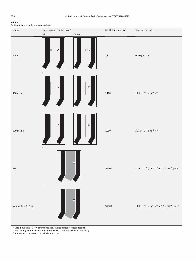
Table 1Emission source configurations evaluated.

Source Source position in the streeta Width, length, x,y (m) Emission rate (E)

Left Center

Point

b

1,1 0.105 g m�1 s�1

100 m line 1,100 1.05 � 10�3 g m�1 s�1

200 m line

c

1,200 5.25 � 10�4 g m�1 s�1

Area

c

16,300 2.19 � 10�5 g m�2 s�1 or 3.5 � 10�4 g m s�1

Volume (z ¼ 0e2 m) 16,300 1.09 � 10�5 g m�3 s�1 or 3.5 � 10�4 g m s�1

a Black: buildings; Grey: source position; White circle: receptor position.b This configuration corresponds to the HCMC tracer experiment (real case).c Sources that represent the vehicle emissions.

L.C. Belalcazar et al. / Atmospheric Environment 44 (2010) 3814e38223818

Fig. 3. Modeled and observed normalized concentrations of tracer as a function ofbackground wind direction. X corresponds to the average observed normalized valuescalculated from all the data available at the indicated wind direction bin. The standarddeviations of the observed values are shown as vertical bars.

Fig. 4. Tracer distributions over the BTH street at the receptor level (z ¼ 2e3 m). The black asimulation. The emission line and the receptor position are indicated in the center of the fi

L.C. Belalcazar et al. / Atmospheric Environment 44 (2010) 3814e3822 3819

Conversely, model performance was significantly poorer whenwind is parallel to the street axis; in particular the modeledconcentration is significantly underestimated at 210�. At thisdirection wind flows parallel to the street and pushes the tracerdownstream, without reaching the receptor point (Fig. 4). As it waspreviously stated in Section 2.2, the selected domain only covers300 m of the BTH street, it only covers part of the buildings that areat the south-west of the domain (Fig. 1). These buildings shelter thestreet and probably change the flow direction which carries thetracer to the receptor (as at 180�, see Fig. 4). A larger domain mayimprove the results at 210� but it may also increase the computa-tion time. The traffic induced turbulence that is not regarded in themodel may also affect the results because it may widen the tracerplume at this wind direction. Wind meandering may also have aneffect on flow variations within the canyon during averaging times.In any case, as most of the HCMC wind direction data (80%) were

rrows at the bottom of each figure indicate the background wind direction used for thegures.

Fig. 5. Normalized concentrations (C*) as a function of wind directions. Left (a) Emission sources at the left of the street (the 100 m line corresponds to the real case of HCMC). Right(b) Emission sources at the center of the street (hypothetical emission sources).

L.C. Belalcazar et al. / Atmospheric Environment 44 (2010) 3814e38223820

between 60 and 180�, the subsequent simulations are carried outusing only these directions.

Dixon et al. (2006) also evaluated the performance of Win-MISKAM in a street canyon in York, UK. In that evaluation themodelwas able to reproduce the qualitative variations of the observationsbut modeled concentrations were overestimated. Moreover, themodel predicted the maximum concentrations at the wrong winddirection; the maximum modeled concentration at the leewardside was 50% higher than the average observed value. Dixon et al.recommend improving the representation of traffic emission toobtain better results. As wementioned before, in this work we havereduced the error produced by the traffic emissions in the valida-tion process because we know the amount of emission released.This highlight the utility of the method presented in this work tovalidate dispersion models.

As it can be seen, WinMISKAM was able to reproduce very wellthe average behavior of the tracer in the street canyon even thoughit doesn’t consider thermodynamic processes such as energytransformation at the surface of the road, walls, roofs of buildings,thermal dispersion, buoyancy or water balance. In the case ofHCMC, the CFD model produced very good results for oblique andperpendicular flows without considering these parameters of thesimulations. It will be necessary to develop similar studies in othercities of the world and to quantify the real impact of this parameteron the simulation results.

3.2. Phase II: correction of the HCMC EFs

Fig. 5 shows the normalized concentrations (C*) calculated fromequation (3) for all these sources. Two of the sources (area and

Table 2ErrorWD (in %) between the sources configurations evaluated and the volume source(the source that represents the vehicle emissions).a

Winddirection(WD)

100 m line at theleft of the streetb

200 m line atthe left of thestreet

100 m line atthe center of thestreet

200 m line atthe center of thestreet

60 96 74 52 1090 91 68 36 6120 58 50 7 �2150 54 44 16 6180 73 48 25 6

a The error is calculated from equation (4).b Real case in the HCMC tracer experiment.

volume) are used to represent the vehicle emissions. There are verysmall differences between the normalized concentrations obtainedfrom these two sources (Fig. 5). The greatest difference is observedat 60�, at this direction the volume source is 7% smaller than thearea source; in the rest of the cases the differences are smaller than5%. Therefore, in this case any of these sources is able to representthe vehicle emissions. In order to simplify the explanations for theremainder of this paper only the volume source is used.

Fig. 5a shows C* calculated from the source configuration usedin HCMC (100 m line at the left). For 120 and 150�, C* calculatedfrom the HCMC source approximates the trends of the volumesource. From 120 to 180� the error calculated from the HCMCsource is 54e73% (see Table 2), whereas from 60 to 90� it is 91e96%.Moreover, the smallest errors are presented at 120 and 150�, thusonly the errors estimated for these two wind directions are used tocorrect the dispersion factors and the EFs. It is important tomention here that if the EFs are corrected by using all the errorsavailable (60e180�), the EFs are nearly similar to the ones esti-mated by using only the errors from the two wind direction bins(120e150�); but the correlation coefficients decrease substantially.This decrease may be attributed to the increase in the error forwinds that are less perpendicular to the street axis.

Fig. 6 shows the corrected propene emission factor. Table 3presents the VOCs EFs estimated before (q) and after the

Fig. 6. Corrected propene vehicle emission factors (the continuous line is the linearregression fit. CI is the 95% confidence interval).

Table 3HCMC VOCs emission factors (mg veh�1 km�1) and comparison with other studies.

Compound HCMCa q (CI) HCMCb Taipeic Chung-Liaod Taipeie

n Cb R qc (CI)

Propene 19.1 (9%) 175 21.1 0.66 7.6 (34%) 11.6 10.4 23Trans-2-Butene 4.9 (17%) 175 6.1 0.47 2.1 (56%) 1.6 0.81-Butene 4.8 (11%) 175 4.8 0.59 1.9 (41%) 8.3 10.7Cis-2-butene 4.6 (17%) 174 5.7 0.47 2.0 (56%) 1.8 1.6i-Pentane 86.8 (14%) 175 102.2 0.51 34.0 (51%) 12.5 40.1 118n-Pentane 27 (11%) 175 28.9 0.57 9.8 (43%) 9.5 19.3 16Trans-2-Pentene 15.8 (15%) 175 19.0 0.52 7.4 (49%) 2.8 4.11-Pentene 5.5 (12%) 173 4.7 0.57 2.3 (42%) 1.6 12-Methyl-2-butene 4.2 (14%) 175 4.6 0.56 1.9 (44%)Cis-2-Pentene 5.3 (12%) 175 4.4 0.55 2.2 (46%) 1.6 1.62,3-Dimethylbutane 15.2 (11%) 174 11.2 0.56 5.2 (44%) 12.72-Methylpentane 14.6 (12%) 174 10.6 0.44 5.6 (61%) 12.6 223-Methylpentane 70.7 (10%) 175 52.3 0.62 27.4 (38%) 5.6 24n-Hexane 116.9 (16%) 175 106.1 0.51 56.2 (50%) 4.18 5.7Benzene 19.1 (13%) 175 16.6 0.51 7.5 (51%) 12.2 5.9 20

LDV: Light Duty Vehicles (gasoline vehicles); HDV: Heavy Duty Vehicles (diesel vehicles); MC: Motorcycles (gasoline vehicles).a Emission factors (q) and the 95% confidence intervals (CI) before the correction (Belalcazar et al., 2009).b This study. n: Available number of data at the selected wind directions (105e165�); Cb: Background concentration (ppbv); R: correlation coefficient; CI: 95% confidence

intervals. LDV: 99.5% (MC: 95%); HDV: 0.5%.c Taipei tunnel study (Hwa et al., 2002). LDV: 93%; HDV: 7%.d Chung-Liao tunnel (Chiang et al., 2007). LDV: 85%; HDV: 15%.e Dynamometer test (Tsai et al., 2003). Emission factors extracted from Fig. 1 (in use 4-strokes motorcycles).

L.C. Belalcazar et al. / Atmospheric Environment 44 (2010) 3814e3822 3821

correction (qc), together with some statistical parameters, anda comparison with other studies. Since the fleet in HCMC ismostly made of light duty vehicles, results obtained here arecompared to studies with a high proportion of light duty vehiclesin the fleet. Results are compared with VOCs EFs estimated invehicular tunnels (Hwa et al., 2002; Chiang et al., 2007), and withVOCs EFs estimated for 4-stoke in use motorcycles in a dyna-mometer (Tsai et al., 2003). As can be seen, qc are well below q,and qc are at the same level of the EFs reported in the otherstudies. This stresses the importance of the position source onthe estimation of EFs from tracer studies and highlights theutility of the CFD model on the correction. Nevertheless, thehexane EF is well above the EFs reported in the other studies.Few studies have estimated the hexane EF; these results indi-cated that it is necessary to include this pollutant in futureestimations of road traffic EF.

The confidence intervals of qc are higher than the confidenceintervals of q. Note that only 33% of the data are used to estimate qc(data available from 105 to 165�). This reduction may explain theincrease on the confidence interval. It is important to mention thatthe confidence intervals of the EFs are typically not reported. In thiswork it is possible to do it because a large dataset was collectedwith the on-line gas chromatograph.

3.3. Phase III: other source configurations

In this section other source configurations are evaluated (seeTable 1 and Fig. 5). Fig. 5 shows that C* strongly depends on winddirection. The smallest differences between all the evaluatedsources and the volume source occur when wind is perpendicularor almost perpendicular to the street axis (90e150�). The largestdifferences occur when wind is oblique to the street axis (60 and180�); at these wind directions the difference is larger for thesources that are at the left of the street.

Fig. 5 shows that the point source is the configuration thatapproximates to the vehicle emissions most poorly. C* calculatedfrom this source are more than 95% below the C* calculated fromthe volume source in all the cases (Fig. 5a and b).

A 200 m line source placed at the left of the street wouldimprove the results obtained at 60 and 180� from the source used in

HCMC (100 m line placed in the left of the street), but at the otherwind directions the error would keep nearly the same.

The sources located in the center of the street produce resultsthat approximate better the volume source configuration. A 100 mline placed in the center of the street produces better results thaneven a 200 m line placed in the left of the street. The source thatrepresents the best the vehicle emissions is the 200m line placed inthe center of the street (see Fig. 5b and Table 2). For almost all thewind directions investigated the difference between the C* calcu-lated from this source and the volume source is smaller than 10%.

4. Conclusions

In this work we use the CFD code WinMISKAM to evaluate theimpact of different source configurations on the estimation of EFsfrom tracer studies. We used the CFD model to calculate the errorproduced by the source configurations on the dispersion factorsand therefore on the estimated EFs. In addition, we also used themodel to find a tracer source configuration that better representsthe vehicle emissions.

In a first step, the results of the tracer experiment were used toevaluate the performance of the CFD model on simulating thedispersion of the tracer. The results of this evaluation indicate thatthe model is able to simulate quite well the tracer dispersion in thisurban environment. The model reproduces the same averagetrends and levels of the observations in most of the cases. There isa very good performance when wind is perpendicular or oblique tothe street axis. However, the model underestimates the concen-trations when wind is parallel to the street axis. This underesti-mation may be attributed to the size of the chosen simulationdomain. The traffic induced turbulence that is not regarded in themodel may also affect the results because it may widen the tracerplume at this wind direction. Wind meandering may also have aneffect on flow variations within the canyon during averaging times.

The model was also used to estimate the error produced by thesource configuration used in HCMC to estimate the EFs. Thecalculations show that the error is smaller when wind is perpen-dicular or almost perpendicular to the street. These errors wereafterwards used to correct the dispersion factors and to recalculatethe HCMC EFs. A comparison with available studies indicates that

L.C. Belalcazar et al. / Atmospheric Environment 44 (2010) 3814e38223822

the corrected EFs are within the range of the EFs reported inother studies.

In order to find the source configuration that better representsthe vehicle emissions, the CFD model was run using the sameconditions (meteorology, street geometry) but changing the sourceconfigurations. Three source configurations placed in two differentpositions are evaluated; they are a point source, a 100 m line sourceand a 200m line source. All these configurations were placed in oneside and in the center of the street. These configurations includedthe one used in the HCMC tracer experiment (100 m line placed inone side of the street). The simulation results show that a 200 mline place in the center of the street would represent very well thevehicle emissions. It would be very interesting to use a 200 memission source to estimate the EFs in a city.

In conclusion, the methods and techniques presented in thiswork may have different practical applications and their use canprovide valuable information for the urban air quality assessment.Results from the tracer study can be used to estimate the EFs underreal urban conditions and to validate dispersion models which inturn can be used in the future to evaluate abatement strategies forsuch streets. Furthermore, concentrations of pollutants are deter-mined at roadside level, as well as their evolution in time, thisinformation may be used for exposure studies.

Acknowledgments

The authors of this study thank the CS-ULP & REALISE and to theEcole Polytechnique Fédérale de Lausanne e EPFL, for the fundingprovided for this project.

References

Balczó, M., Gromke, Ch, Ruck, B., 2009. Numerical modeling of flow and pollutantdispersion in street canyons with tree planting. Meteorologische Zeitschrift 18,197e206.

Belalcazar, L.C., Fuhrer, O., Ho, D., Zarate, E., Clappier, A., 2009. Estimation of roadtraffic emission factors from a long term tracer study in Ho Chi Minh City(Vietnam). Atmospheric Environment 43, 5830e5837.

Benson, J., Ziehn, T., Dixon, N.S., Tomlin, A.S., 2008. Global sensitivity analysis of a 3-dimensional street canyon model e part II: application and physical insightusing sensitivity analysis. Atmospheric Environment 42, 1874e1891.

Chiang, H., Hwu, C., Chen, S., Wu, M., Ma, S., Huang, Y., 2007. Emission factors andcharacteristics of criteria pollutants and volatile organic compounds (VOCs) ina freeway tunnel study. Science of the Total Environment 381, 200e211.

Dixon, N.S., Boddy, J.W.D., Smalley, R.J., Tomlin, A.S., 2006. Evaluation of a turbulentflow and dispersion model in a typical street canyon in York, UK. AtmosphericEnvironment 40, 958e972.

Donnelly, R.P., Lyons, T.J., Flassak, T., 2009. Evaluation of results of a numericalsimulation of dispersion in an idealised urban area for emergency responsemodelling. Atmospheric Environment 43, 4416e4423.

Eichhorn, J., 2008. WinMISKAM for Windows Manual (Version 5.02). Institute forAtmospheric Physics, University of Mainz, Germany.

Eichhorn, J., Kniffka, A., 2010. The numerical flowmodelMISKAM: state of developmentand evaluation of the basic version. Meteorologische Zeitschrift 19 (1), 081e090.

Franke, J., Hellsten, A., Schlünzen, H., Carissimo, B. (Eds.), 2007. Best PracticeGuideline for the CFD Simulation of Flows in the Urban Environment COSTAction 732, Quality Assurance and Improvement of Microscale MeteorologicalModels.

Gidhagen, L., Johansson, C., Langner, J., Olivares, G., 2004. Simulation of NOx andultrafine particles in a street canyon in Stockholm, Sweden. AtmosphericEnvironment 38, 2029e2044.

Gramotnev, G., Brown, R., Ristovski, Z., Hitchins, J., Morawska, L., 2002. Determi-nation of average emission factors for vehicles on a busy road. AtmosphericEnvironment 37, 465e474.

Holmes, N., Morawska, L., 2006. A review of dispersion modeling and its applicationto the dispersion of particles: an overview of different dispersion modelsavailable. Atmospheric Environment 40, 5902e5928.

Hwa, M., Hsieh, C., Wu, T., Chang, L., 2002. Real-world vehicle emissions and VOCsprofile in the Taipei tunnel located at Taiwan Taipei area. Atmospheric Envi-ronment 36, 1993e2002.

Kastner-Klein, P., Fedorovich, E., Ketzel, M., Berkowicz, R., Britter, R., 2003. Themodelling of turbulence from traffic in urban dispersion models e part II:evaluation against laboratory and full-scale concentration measurements instreet canyons. Environmental Fluid Mechanics 3, 145e172.

Kawashima, H., Minami, S., Hanai, Y., Fushimi, A., 2006. Volatile organic compoundemission factors from roadside measurements. Atmospheric Environment 40,2301e2312.

Ketzel, M., Berkowicz, R., Lohmeyer, A., 2000. Comparison of numerical streetdispersion models with results from wind tunnel and field measurements.Environmental Monitoring and Assessment 65, 363e370.

Ketzel, M., Wåhlin, P., Berkowicz, R., Palmgren, F., 2003. Particle and trace gasemission factors under urban driving conditions in Copenhagen based on streetand roof-level observations. Atmospheric Environment 37, 2735e2749.

Kumar, P., Garmory, A., Ketzel, M., Berkowicz, R., Britter, R., 2009. Comparative studyof measured and modelled number concentrations of nanoparticles in an urbanstreet canyon. Atmospheric Environment 43, 949e958.

Li, X., Liu, C., Leung, D., Lam, K., 2006. Recent progress in CFD modelling of windfield and pollutant transport in street canyons. Atmospheric Environment 40,5640e5658.

Lohmeyer, A., Mueller, W.J., Baechlin, W., 2002. A comparison of street canyonconcentration predictions by different modelers: final results now availablefrom the Podbi-exercise. Atmospheric Environment 36, 157e158.

Meroney, R.N., Pavageau, M., Rafailidis, S., Schatzmann, M., 1996. Study of linesource characteristics for 2-D physical modelling of pollutant dispersion instreet canyons. Journal of Wind Engineering and Industrial Aerodynamics 62,37e56.

Molina, M., Molina, L., 2004. Megacities and atmospheric pollution. Air and WasteManagement Association 54, 644e680.

Olesen, H.R., Berkowicz, R., Ketzel, M., Løfstrøm, P., 2009. Validation of OML, AER-MOD/PRIME and MISKAM using the Thompson wind-tunnel dataset for simplestack-building configurations. Boundary-Layer Meteorology 131, 73e83.

Palmgren, F., Berkowicz, R., Ziv, A., Hertel, O., 1999. Actual car fleet emissionsestimated from urban air quality measurements and street pollution models.Science of the Total Environment 235, 101e109.

Tsai, J., Liu, Y., Yang, C., 2003. Volatile organic profiles and photochemical potentialsfrom motorcycle engine exhaust. Air and Waste Management Association 53,516e522.

Vardoulakis, S., Fisher, B.E.A., Pericleous, K., Gonzalez-Flesca, N., 2003. Modelling airquality in street canyons: a review. Atmospheric Environment 37, 155e182.

VDI 3783/9, 2005. Prognostic Microscale Wind Field Models. Evaluation for FlowAround Buildings and Obstacles. Beuth-Verlag, Berlin, 53 pp.

Yoshimura, M., Yamashita, M., Ichie, T., 2006. Light environmental monitoring intropical rainforest. Proceedings of the Asian Conference on Remote Sensing(ACRC).

Zárate, E., Belalcázar, Luis., Clappier, A., Manzi, V., Van den Bergh, H., 2007.Air quality modelling over Bogota, Colombia: combined techniques toestimate and evaluate emission inventories. Atmospheric Environment 41,6302e6318.