An Equilibrium Model of Habitat Conservation under Uncertainty and Irreversibility NOTA DI LAVORO 160.2010 By Luca Di Corato, Department of Economics, Swedish University of Agricultural Sciences Michele Moretto, Department of Economics, University of Padova, Fondazione Eni Enrico Mattei and Centro Studi Levi-Cases, Italy Sergio Vergalli, Department of Economics, University of Brescia and Fondazione Eni Enrico Mattei, Italy

Welcome message from author
This document is posted to help you gain knowledge. Please leave a comment to let me know what you think about it! Share it to your friends and learn new things together.
Transcript
An Equilibrium Model of Habitat Conservation under Uncertainty and Irreversibility
NOTA DILAVORO160.2010
By Luca Di Corato, Department of Economics, Swedish University of Agricultural Sciences Michele Moretto, Department of Economics, University of Padova, Fondazione Eni Enrico Mattei and Centro Studi Levi-Cases, Italy Sergio Vergalli, Department of Economics, University of Brescia and Fondazione Eni Enrico Mattei, Italy
The opinions expressed in this paper do not necessarily reflect the position of Fondazione Eni Enrico Mattei
Corso Magenta, 63, 20123 Milano (I), web site: www.feem.it, e-mail: [email protected]
SUSTAINABLE DEVELOPMENT Series Editor: Carlo Carraro
An Equilibrium Model of Habitat Conservation under Uncertainty and Irreversibility By Luca Di Corato, Department of Economics, Swedish University of Agricultural Sciences Michele Moretto, Department of Economics, University of Padova, Fondazione Eni Enrico Mattei and Centro Studi Levi-Cases, Italy Sergio Vergalli, Department of Economics, University of Brescia and Fondazione Eni Enrico Mattei, Italy Summary In this paper stochastic dynamic programming is used to investigate habitat conservation by a multitude of landholders under uncertainty about the value of environmental services and irreversible development. We study land conversion under competition on the market for agricultural products when voluntary and mandatory measures are combined by the Government to induce adequate participation in a conservation plan. We analytically determine the impact of uncertainty and optimal policy conversion dynamics and discuss different policy scenarios on the basis of the relative long-run expected rate of deforestation. Finally, some numerical simulations are provided to illustrate our findings. Keywords: Optimal Stopping, Deforestation, Payments For Environmental Services, Natural Resources Management JEL Classification: C61, D81, Q24, Q58 Address for correspondence: Luca Di Corato Department of Economics Swedish University of Agricultural Sciences Box 7013, Johan Brauners väg 3, Uppsala, 75007 Sweden Phone: +46018671758 Fax: +46018673502 E-mail: [email protected]
An Equilibrium Model of Habitat Conservation underUncertainty and Irreversibility�
Luca Di Coratoy Michele Morettoz Sergio Vergallix
December 3, 2010
Abstract
In this paper stochastic dynamic programming is used to investigate habitat conservation by a mul-titude of landholders under uncertainty about the value of environmental services and irreversible de-velopment. We study land conversion under competition on the market for agricultural products whenvoluntary and mandatory measures are combined by the Government to induce adequate participation ina conservation plan. We analytically determine the impact of uncertainty and optimal policy conversiondynamics and discuss di¤erent policy scenarios on the basis of the relative long-run expected rate ofdeforestation. Finally, some numerical simulations are provided to illustrate our �ndings.keywords: optimal stopping, deforestation, payments for environmental services, NaturalResources Management.jel classification: C61, D81, Q24, Q58.
1 Introduction
As human population grows, the human-Nature con�ict has become more severe and natural habitats aremore exposed to conversion. On the one hand, clearing land to develop it may lead to the irreversiblereduction or loss of valuable environmental services (hereafter, ES) such as biodiversity conservation, carbonsequestration, watershed control and provision of scenic beauty for recreational activities and ecotourism.On the other hand, conserving land in its pristine state has a cost opportunity in terms of foregone pro�tsfrom economic activities (e.g. agriculture, commercial forestry) which can be undertaken once land has beencleared.By balancing marginal social bene�t and cost of conservation, the social planner is required to destine
the available land to conservation or development which are usually two competing and mutually exclusiveuses. Despite its theoretical appeal, the idea of a social planner who, having de�ned a socially optimalhabitat conversion rule, can implement it by simply commanding the constitution of protected areas, is farfrom reality. In fact, since the majority of remaining ecosystems are on land privately owned, the economicand political cost of such intervention would make the adoption of command mechanisms by Governmentsunlikely (Langpap and Wu, 2004; Sierra and Russman, 2006). In addition, as pointed out by Folke etal.(1996, p. 1019), "keeping humans out of nature through a protected-area strategy may buy time, but itdoes not address the factors in society driving the loss of biodiversity". In other words, protecting naturalecosystems through natural reserves and other protected areas may be a signi�cant step in the short-run todeal with severe and immediate threats but it still does not create the structure of incentives able to mitigatethe con�ict human-Nature in the long-run.At least initially, Governments favoured an indirect approach in conservation policies. The main idea
behind this approach was to divert, through programs such as integrated conservation and development�We wish to thank Guido Candela for helpful comments. We are also grateful for comments and suggestions to participants
at the 12th International BIOECON and 51st SIE conferences and to seminars at FEEM & IEFE - Bocconi University and atDept of Economics Seminars, University of Stirling. The usual disclaimer applies.
yCorresponding address: Department of Economics, Swedish University of Agricultural Sciences, Box 7013, Johan Braunersväg 3, Uppsala, 75007, Sweden. Email: [email protected]. Telephone: +46(0)18671758. Fax: +46(0)18673502.
zDepartment of Economics, University of Padova, Fondazione Eni Enrico Mattei and Centro Studi Levi-Cases, Italy.xDepartment of Economics, University of Brescia, and Fondazione Eni Enrico Mattei, Italy.
1
projects, community-based natural resource management or other environment-friendly commercial ven-tures, the allocation of labour and capital from ecosystem damaging activities toward ecosystem conservingactivities (Wells et al., 1992; Ferraro and Simpson, 2002). However, despite the initial enthusiasm, e¤ec-tiveness and cost-e¢ ciency concerns have led to abandonment of this approach in favour of compensationsto be paid directly to the landholders providing conservation services (see e.g. Ferraro, 2001; Ferraro andKiss, 2002; Ferraro and Simpson, 2005). A direct approach, mainly represented by schemes like Paymentsfor environmental services (hereafter, PES) has become increasingly common in both developed and devel-oping countries. Under a PES program, a provider delivers to a buyer a well-de�ned ES (or correspondingland use) in exchange for an agreed payment.1 Unfortunately, also the e¢ cacy of PES programs has beenquestioned since their performance has not always met the established conservation targets.2 In particular,lack of additionality in the conservation e¤orts induced by the programs has often been suspected.3 In otherwords, it seems that in practice landholders have been practically paid for conserving the same extent of landthey would have conserved without the program. Considering the limited amount of money for conservationinitiatives and the perverse e¤ect that wasting it may have on future funding, further research is needed toincrease our understanding of the economic agent�s conversion decision.The literature investigating optimal conservation decisions under irreversibility and uncertainty over the
net bene�ts attached to conservation represents a signi�cant branch of environmental and resource economics(Bulte et al., 2002, Kassar and Lassere, 2004; Leroux et al., 2009). A unifying aspect in this literature is thestress on the e¤ect that irreversibility and uncertainty have on decision making. In fact, since irreversibleconversion under uncertainty over future prospects may be later regretted, this decision may be postponedto bene�t from option value attached to the maintained �exibility (Dixit and Pindyck, 1994). Pioneer paperssuch as Arrow and Fisher (1974) and Henry (1974) have been followed by several other contributions whichhave improved the modelling e¤ort and solved the technical problems posed by increasingly complex modelset-up.4 Two contributions close to ours are Bulte et al. (2002) and Leroux et al. (2009). In the �rst paper,the authors determine the optimal forest stock to be held by trading o¤ pro�t from agriculture and the valueof ES attached to forest conservation. Their analysis highlights the value of the option to postpone landclearing under irreversibility of environmental impact and uncertainty about conservation bene�ts. A similarproblem is solved in Leroux et al. (2009) where, unlike the previous paper, the authors allow for ecologicalfeedback and consider its impact both on the expected trend and volatility of ES value.Both papers, however, by solving the allocative problem from a central planner perspective, miss the
complexity of challenges characterizing conservation policies and the role that competition on markets foragricultural products may have on conversion decisions.In this paper, we aim to investigate these issues by modelling conversion decisions in a decentralized
economy populated by a multitude of homogenous landholders and where the Government has introduceda payment scheme for conservation. Each landholder manages a portion of total available land and mayconserve or develop it by a¤ording some conversion cost. If land is conserved, ES have a value proportionalto the area conserved which randomly �uctuates following a geometric Brownian motion. If the parcel isdeveloped, land enters as an input into the production of goods or services (co¤ee, rubber, soy, palm oil,timber, biofuels, cattle, etc.) and the farmer must compete with other farmers on the market. In thiscontext, the Government introduces a land use policy which aims to balance conservation and development.The policy is based on a PES scheme implemented through a conservation contract establishing di¤erent
requirements and payments before and after land conversion has occurred. In particular, if the entire plot isconserved, then the landholder receives a certain payment whereas if he/she decides to clear it, then he/shemust set aside the portion indicated in the contract (i.e. the plot may be only partially developed) andreceives a di¤erent payment. Finally, we also consider the possibility that the Government may impose a
1 In this respect we follow Wunder (2005, p. 3) where a PES is de�ned as "(i) a voluntary transaction where (ii) a well-de�nedES (or a land-use likely to secure that service) (iii) is being "bought" by a (minimum one) ES buyer (iv) from a (minimum one)ES provider (v) if and only if the ES provider secures ES provision (conditionality)".
2As reported by Ferraro (2001), this may be due to several reasons such as lack of funding, failures in institutional design,poor de�nition and weak enforcement of property rights and strategic behaviour by potential ES providers. See Ferraro (2008)on information failures and Smith and Shogren (2002) on speci�c contract design issues.
3We refer in particular to government-�nanced programs. On the performance of user vs. government-�nanced interventionssee Pagiola (2008) on PSA program in Costa Rica and Wunder et al. (2008) for a comparative analysis of PES programsin developed and developing countries. See Ferraro and Pattanayak (2006) for a call on empirical monitoring of conservationprograms.
4Among them, see for instance Conrad (1980), Clarke and Reed (1989), Reed (1993), Conrad (1997), Conrad (2000).
2
limit on the total forested land which can be cleared.Under this conservation program we solve for the conversion path taking a real option approach but
unlike from previous literature we internalize the role of market entry dynamics. It follows that undercompetition the conversion path must be determined on the basis of a long-run zero pro�t condition. Inthis respect, it becomes interesting to study the impact that di¤erent payment scheme may have on theconversion dynamic. We then allow for two di¤erent PES schemes. Under the �rst one, the payment ratefor land unit is more generous when the entire plot is conserved while in the second scheme the opposite isproposed. Both situations may arise in reality, re�ecting di¤erent sensitivity towards conservation or, morepractically, the way Governments try to adapt to the economic and political framework they face.5
Under both schemes, we are able to determine analytically the optimal conversion rules. Not surprisingly,conversion is postponed if landholders conserving the entire plot receive a higher payment. This is due tothe higher cost opportunity of conversion which is higher since it includes the payments implicitly givenup converting. Interestingly, we show that, as suggested by Ferraro (2001), a landholder may conserve theentire plot even if partially compensated for the provided ES. Moreover, under this payment design, onlyprogressive reductions in the payments trigger land clearing and, at the end, landholders may clear a surfacesmaller than the one targeted by the Government. With the second payment design, i.e. higher transfer ifland is developed, the structure of incentives is reversed and an implicit bias toward conversion is introduced.An important mass of landholders rapidly convert land till the last plot where pro�t from agriculture coversthe conversion cost while the rest prefers to wait and clear the plots only if payments rise. Under bothPES designs, we note that, by setting a limit to the land surface that landholders may develop together, theGovernment may induce rush in the conversion dynamics.6 In fact, landholders, fearing a restriction in theexercise of the option to convert, may start a conversion run which rapidly exhausts the entire forest stockup to the �xed limit.7
Finally, to assess the temporal performance of the optimal conservation policy and study the impact ofincreasing uncertainty about future environmental bene�ts on conversion speed, we rearrange the optimalconversion rules in the form of regulated processes (Harrison, 1985, chp. 2) and derive the long-run averagegrowth rate of deforestation. Hence, under di¤erent policy scenarios, we use the rate of deforestation torank di¤erent policies on the basis of current optimal forest stock and expected total conversion time.Interestingly, we show that uncertainty about payments, even if it induces conversion postponement in theshort-run, reduces expected time for total conversion in the long run.We then use it to illustrate, through several numerical simulations, optimal forest conversion in Costa
Rica.8 We �nd that when landholders conserving the whole plot are o¤ered a higher payment with respect tothe ones developing, then higher uncertainty over payments increases the long-run average rate of conversion.The opposite occurs when the policy rewards more generously farmers conserving only a portion of theirplot.The remainder of the paper is organized as follows. In Section 2 the basic set-up for the model is
presented. In Section 3 we study the equilibrium in the conversion strategies under two policy scenarios. InSection 4, we discuss issues related to the PES voluntary participation and contract enforceability. Section5 is devoted to the derivation of the long-run average rate of conversion. In Section 6 we illustrate our main�ndings through numerical exercises. Section 7 concludes.
5For instance, if forest conservation does not qualify under the CDM (Clean Development Mechanism) while reforestationdoes, then it may be plausible for a Government to push towards timber harvest and subsequent reforestation on some land inorder to cash funding on carbon markets and �nance conservation on the remaining habitat. Note that this was actually thecase in the �rst commitment period (2008-2012) (IPCC, 2007).
6 In Australia, the Productivity Commission reports evidence of pre-emptive clearing due to the introduction of clearingrestrictions (Productivity Commission, 2004). On unintended impacts of public policy see for instance Stavins and Ja¤e (1990)showing that, despite an explicit federal conservation policy, 30% of forested wetland conversion in the Mississippi Valley hasbeen induced by federal �ood-control projects. In this respect, see also Mæstad (2001) showing how timber trade restrictionsmay induce an increase in logging.
7A similar e¤ect has been �rstly noted by Bartolini (1993). In this paper, the author studies decentralized investment decisionin a market where a limit on aggregate investment is present.
8Unlike Leroux et al. (2009) who exogenously assume a maximum annual conversion rate (2.5% in the case of Costa Ricaforests), we calculate it optimally on the basis of land currently converted and information on current and future payments.
3
2 A Dynamic Model of Land Conversion
Consider a country where at time period t = 0 the total land available, L, is allocated as follows:
L = A0 + F (1)
where A0 is the surface cultivated and F is the portion still in its pristine natural state covered by primaryforest.9 Assume that F is divided into small and homogenous parcels of equal extent held by a multitude ofidentical risk-neutral agents.10 By normalizing such extent to 1 hectare, F denotes also the number of agentsin the economy.11 Natural habitats provide valuable environmental goods and services at each time periodt.12 Let B(t) represent the per-parcel value of such goods and services and assume it randomly �uctuatesaccording to the following geometric Brownian motion:
dB(t)
B(t)= �dt+ �dz(t); with B(0) = B (2)
where � and � are respectively the drift and the volatility parameters, and dz(t) is the increment of a Wienerprocess.13
At each t, two competitive and mutually exclusive destinations may be given to forested land: conservationor irreversible development. Once the plot is cleared, the landholder becomes a farmer using land as an inputfor agricultural production (or commercial forestry).14
2.1 The Government
To induce conservation the Government o¤ers to each agent a contract to be accepted on a voluntary basis.A compensation equal to �1B(t) with �1 2 [0; 1] is paid at each time period t if the entire plot is conserved.15On the contrary, if the landholder aims to develop his/her parcel, a restriction is imposed in that a portionof the total surface, 0 � � � 1, must be conserved.16 In this case, a payment equal to ��2B(t) with�2 2 [0; 1] may be o¤ered to compensate the landholder.17 Since ES usually have the nature of public good,payment rates, �1 and �2, may be interpreted as the levels of appropriability that the society is willing to
9As in Bulte et al. (2002) A0 may represent the best land which has been converted to agriculture.10At the moment for the sake of generality we refer to landholders. Later we will discuss the implications of our model with
respect to property rights issues.11None of our results relies on this assumption. In fact, provided that no single agent has signi�cant market power, we can
obtain identical results by allowing each agent to own more than one unit of land. See e.g. Baldursson (1998) and Grenadier(2002).12They may include biodiversity conservation, carbon sequestration, watershed control, provision of scenic beauty for recre-
ational activities and ecotourism, timber and non-timber forest products. See e.g. Conrad (1997), Conrad (2000), Clarke andReed (1989), Reed (1993), Bulte et al. (2002).13The Brownian motion in (2) is a reasonable approximation for conservation bene�ts and we share this assumption with
most of the existing literature. Conrad (1997, p. 98) considers a geometric Brownian motion for the amenity value as a plausibleassumption to capture uncertainty over individual preferences for amenity. Bulte et al. (2002, p.152) point out that "parameter� can be positive (e.g., re�ecting an increasingly important carbon sink function as atmospheric CO2 concentration rises), butit may also be negative (say, due to improvements in combinatorial chemistry that lead to a reduced need for primary geneticmaterial)". However, this assumption neglects the direct feedback e¤ect that conversion decisions may have on the stochasticprocess illustrating the dynamic of conservation bene�ts. See Leroux et al. (2009) for a model where such e¤ect is accountedby letting conservation bene�ts follow a controlled di¤usion process with both drift and volatility depending on the conversionpath.14 In the following, "landholder" refers to an agent conserving land and "farmer" to an agent cultivating it.15As pointed out by Engel et al. (2008), by internalizing external non-market values from conservation, PES schemes have
attracted increasing interest as mechanisms to induce the provision of ES.16Note that our analysis is general enough to include also the case where � is not imposed but is endogenously set by each
landholder. In fact, due for instance to �nancial constraints limiting the extent of the development project, the landholdersmay �nd optimal not to convert the entire plot.17Note that our contract scheme is in line with Ferraro (2001, p. 997) where the author states that conservation practitioners
"may also �nd that they do not need to make payments for an entire targeted ecosystem to achieve their objectives. Theyneed to include only "just enough" of the ecosystem to make it unlikely, given current economic conditions, infrastructure, andenforcement levels, that anyone would convert the remaining area to other uses". In addition, taking a di¤erent perspective,our framework seems supported also by wildlife protection programs which rarely pay farmers more than a fraction of the lossesdue to wildlife (See Rondeau and Bulte, 2007).
4
guarantee on the value generated by conserving, i.e. B(t) and �B(t) respectively.18 In addition, besides � theGovernment �xes an upper level �A on total land conversion. This limit may preclude land development forsome landholders. The number of landholders for whom conserving the entire plot may become compulsorydepends on the magnitude of �. In fact, note that � may be low enough to allow every landholder toclear land. However, the de�nition of � does not need to meet such requirement since other issues may beprioritized, i.e. habitat fragmentation, critical ecological thresholds, enforcement and transaction costs forthe program implementation, etc. Thus, denoting by �N =
�A1�� the number of potential farmers involved in
the conversion process, we assume �N � F .
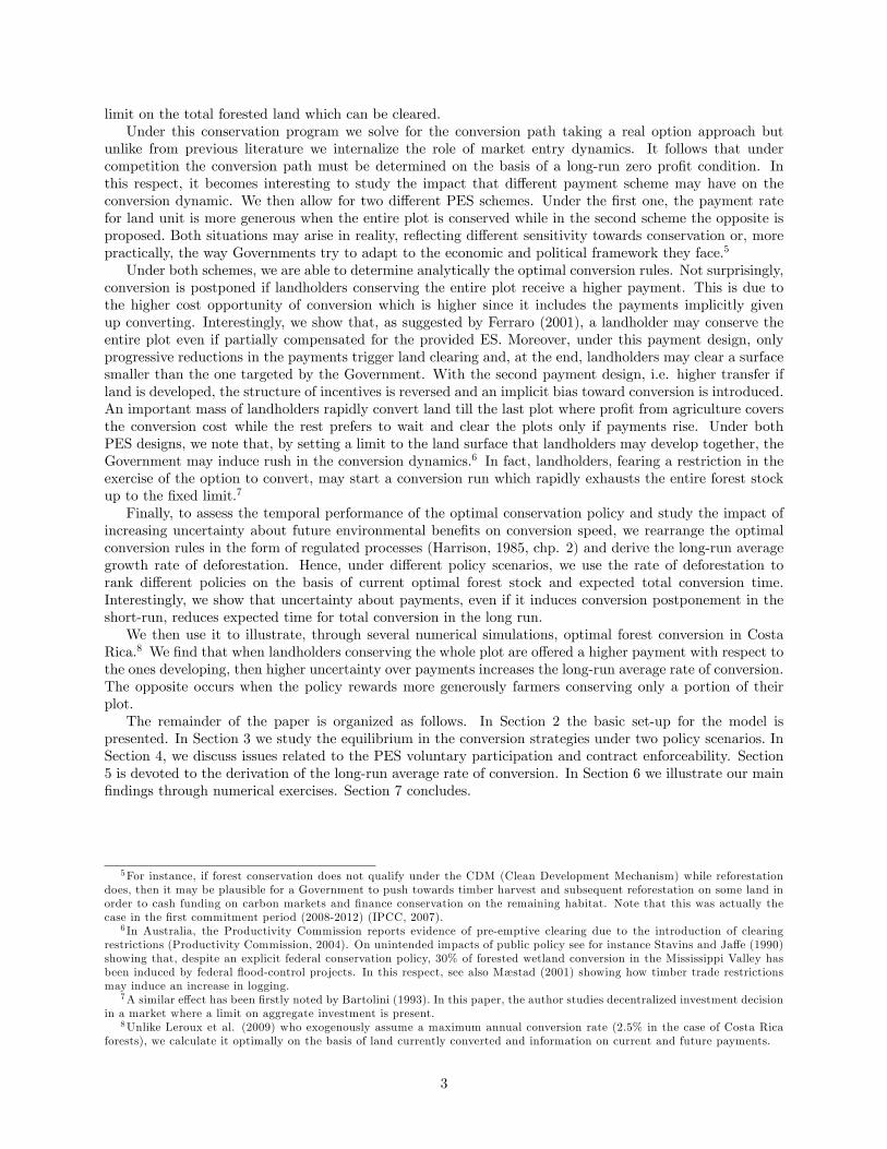
Figure 1: Land conversion with bu¤er areas
Our framework is general enough to include di¤erent conservation targets such as old-growth forests or habitatsurrounding wetlands, marshes, lagoons or by the marine coastline and meet several spatial requirements.For instance, the conservation target may be represented by an area divided into homogenous parcels runningalong a river or around a lake or a lagoon where, to maintain a signi�cant provision of ecosystem services,a portion of each parcel must be conserved (see �gure 1). As stressed by the literature in spatial ecology,the creation of bu¤er areas, by managing the proximity of human economic activities, is crucial since itguarantees the e¢ ciency of conservation measures in the targeted areas.19 In this case the conservationprogram may be induced by implementing a payment contract schedule di¤erentiating for the state of landi.e. totally conserved vs. developed within the restriction enforced through environmental law. However,we are also able to consider the opposite case where the landholder may totally develop his/her plot but anupper limit is �xed on the total extent of land which can be cleared in the region.20
2.2 The Landholders
Developing the parcel is an irreversible action which has a sunk cost, (1��)c, including cost for clearing andsettling land for agriculture.21 Denoting by A(t) the total land developed at time t, the number of farmers18As �1 and �2 are constant, payments also follow a geometric Brownian motion (easily derivable from (2)). However, this
is di¤erent from the way payments are modelled in Isik and Yang (2004) where they also depend on the �uctuations in theconservation cost opportunity (pro�t from agriculture, changes in environmental policy, etc.).19See for instance Hansen and Rotella (2002) and Hansen and DeFries (2007).20This could be the case for an area covered by a tropical forest (Bulte et al., 2002; Leroux et al., 2009), or a protected area
where farmers located next to the site may sustainably extract natural resources (Tisdell, 1995; Wells et al., 1992).21Bulte et al., (2002, p. 152) de�ne c as "the marginal land conversion cost". It "may be negative if there is a positive
one-time net bene�t from logging the site that exceeds the costs of preparing the harvested site for crop production". We also
5
must be equal to N(t) = A(t)1�� and since 1� � is �xed, the conversion dynamic must mirror the variation in
the number of farmers, i.e. dN(t) = dA(t)1�� . Therefore, assuming that the extent of each plot is small enough
to exclude any potential price-making consideration, we may use either N(t) or A(t) when evaluating theindividual decision process.22 Competition on the market for agricultural products implies that at each timeperiod t the optimal number of farmers (or the optimal total land developed) is determined by the entryzero pro�t condition. In addition, since the per-parcel value of services, B(t), makes all agents symmetric,some random mechanism must be used to select which landholder develops �rst.We assume a constant elasticity demand function for agricultural products. Since supply depends on the
surface cultivated, then let demand be speci�ed as PA(t) = �A(t)� with A(0) = A0(> 1), where � is aparameter illustrating di¤erent positions of the demand and � is the inverse of the demand elasticity.Now, let�s solve for the conversion process taking �1, �2 and � as exogenously given parameters. Denoting
by PA(t) the marginal return as land is cleared over time, the farmer instantaneous pro�t function is givenby:
�(A(t); B(t); �A) = (1� �)PA(t) + ��2B(t) (3)
The discounted present value of the net bene�ts over an in�nite horizon is:23
E0
�Z t
0
�1B(t)e�rtdt +
Z 1
t
�(A(t); B(t); �A)e�rtdt
�= (4)
=�1B
r � � + E0�Z 1
t
��(A(t); B(t); �A)e�r(t�t)dt
�where r is the constant risk-free interest rate,24 ��(A(t); B(t); �A)=(1 � �)PA(t) + (��2 � �1)B(t) and t isthe stochastic conversion time.25
In (4) the �rst term represents the perpetuity paid by the Government if the parcel is conserved forever,while the second term represents the extra pro�t that each landholder may expect if she/he clears the landand becomes a farmer. The extra pro�t is, given by the crop yield sold on the market plus the di¤erencein the payments received by the Government. As soon as the excess pro�t from land development equalsthe deforestation cost the landholder may clear the parcel. This implies that the optimal conversion timingdepends only on the second term in (4).
assume, without loss of generality, that the conversion cost is proportional to the surface cleared.22To consider in�nitesimally small agents is a standard assumption in in�nite horizon models investigating dynamic industry
equilibrium under competition. See for instance Jovanovic (1982), Dixit (1989), Hopenhayn (1992), Lambson (1992), Dixit andPindyck (1994, chp. 8), Bartolini (1993), Caballero and Pindyck (1996), Dosi and Moretto (1992) and Moretto (2008).23See Harrison (1985, p. 44).24The introduction of risk aversion does not change the results since the analysis can be developed under a risk-neutral
probability measure for B(t). See Cox and Ross (1976) for further details.25Note that the expected value is taken accounting for A(t) increasing over time as land is cleared.
6
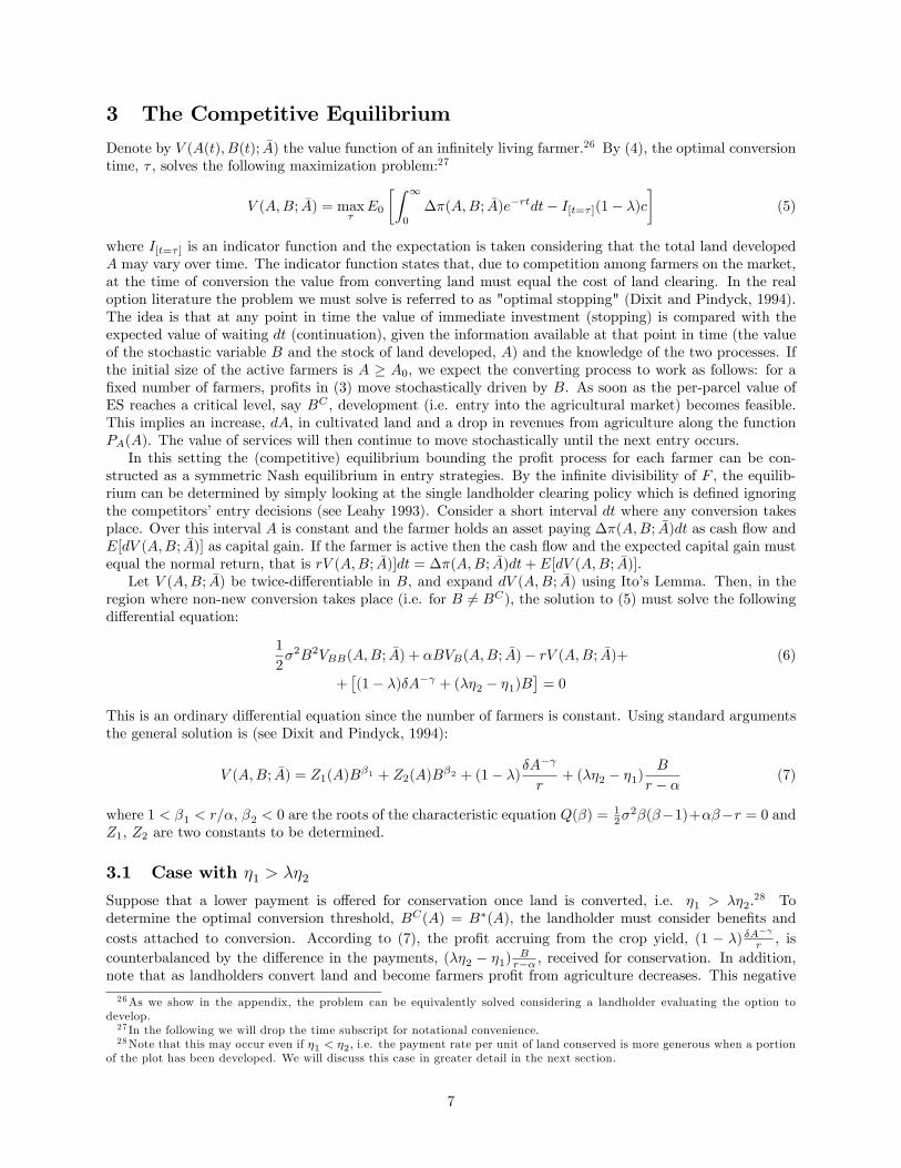
3 The Competitive Equilibrium
Denote by V (A(t); B(t); �A) the value function of an in�nitely living farmer.26 By (4), the optimal conversiontime, � , solves the following maximization problem:27
V (A;B; �A) = max�E0
�Z 1
0
��(A;B; �A)e�rtdt� I[t=� ](1� �)c�
(5)
where I[t=� ] is an indicator function and the expectation is taken considering that the total land developedA may vary over time. The indicator function states that, due to competition among farmers on the market,at the time of conversion the value from converting land must equal the cost of land clearing. In the realoption literature the problem we must solve is referred to as "optimal stopping" (Dixit and Pindyck, 1994).The idea is that at any point in time the value of immediate investment (stopping) is compared with theexpected value of waiting dt (continuation), given the information available at that point in time (the valueof the stochastic variable B and the stock of land developed, A) and the knowledge of the two processes. Ifthe initial size of the active farmers is A � A0, we expect the converting process to work as follows: for a�xed number of farmers, pro�ts in (3) move stochastically driven by B. As soon as the per-parcel value ofES reaches a critical level, say BC , development (i.e. entry into the agricultural market) becomes feasible.This implies an increase, dA, in cultivated land and a drop in revenues from agriculture along the functionPA(A). The value of services will then continue to move stochastically until the next entry occurs.In this setting the (competitive) equilibrium bounding the pro�t process for each farmer can be con-
structed as a symmetric Nash equilibrium in entry strategies. By the in�nite divisibility of F , the equilib-rium can be determined by simply looking at the single landholder clearing policy which is de�ned ignoringthe competitors�entry decisions (see Leahy 1993). Consider a short interval dt where any conversion takesplace. Over this interval A is constant and the farmer holds an asset paying ��(A;B; �A)dt as cash �ow andE[dV (A;B; �A)] as capital gain. If the farmer is active then the cash �ow and the expected capital gain mustequal the normal return, that is rV (A;B; �A)]dt = ��(A;B; �A)dt+ E[dV (A;B; �A)].Let V (A;B; �A) be twice-di¤erentiable in B, and expand dV (A;B; �A) using Ito�s Lemma. Then, in the
region where non-new conversion takes place (i.e. for B 6= BC), the solution to (5) must solve the followingdi¤erential equation:
1
2�2B2VBB(A;B; �A) + �BVB(A;B; �A)� rV (A;B; �A)+ (6)
+�(1� �)�A� + (��2 � �1)B
�= 0
This is an ordinary di¤erential equation since the number of farmers is constant. Using standard argumentsthe general solution is (see Dixit and Pindyck, 1994):
V (A;B; �A) = Z1(A)B�1 + Z2(A)B
�2 + (1� �)�A�
r+ (��2 � �1)
B
r � � (7)
where 1 < �1 < r=�, �2 < 0 are the roots of the characteristic equation Q(�) =12�
2�(��1)+���r = 0 andZ1, Z2 are two constants to be determined.
3.1 Case with �1 > ��2Suppose that a lower payment is o¤ered for conservation once land is converted, i.e. �1 > ��2.
28 Todetermine the optimal conversion threshold, BC(A) = B�(A), the landholder must consider bene�ts andcosts attached to conversion. According to (7), the pro�t accruing from the crop yield, (1 � �) �A�
r , iscounterbalanced by the di¤erence in the payments, (��2 � �1) B
r�� , received for conservation. In addition,note that as landholders convert land and become farmers pro�t from agriculture decreases. This negative
26As we show in the appendix, the problem can be equivalently solved considering a landholder evaluating the option todevelop.27 In the following we will drop the time subscript for notational convenience.28Note that this may occur even if �1 < �2; i.e. the payment rate per unit of land conserved is more generous when a portion
of the plot has been developed. We will discuss this case in greater detail in the next section.
7
e¤ect on the value of converted land is accounted for in (7) by the second term (Z2(A) � 0 for A � �A). Infact, since �1 > ��2 then only an expected reduction in B can induce conversion. This implies that to keepV (A;B; �A) �nite we must drop the �rst term by setting Z1 = 0, i.e. limB!1 V (A,B; �A) = 0. Hence, (7)reduces to:
V (A;B; �A) = Z2(A)B�2 + (1� �)�A
�
r+ (��2 � �1)
B
r � � (8)
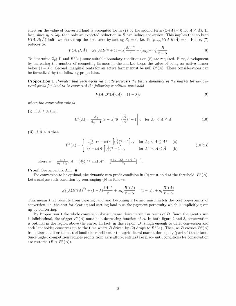
To determine Z2(A) and B�(A) some suitable boundary conditions on (8) are required. First, developmentby increasing the number of competing farmers in the market keeps the value of being an active farmerbelow (1 � �)c. Second, marginal rents for an active farmer must be null B�(A). These considerations canbe formalized by the following proposition.
Proposition 1 Provided that each agent rationally forecasts the future dynamics of the market for agricul-tural goods for land to be converted the following condition must hold
V (A;B�(A); �A) = (1� �)c (9)
where the conversion rule is
(i) if A � �A then
B�(A) =�2
�2 � 1(r � �)
"(A
A) � 1
#c for A0 < A � A (10)
(ii) if A > �A then
B�(A) =
8<:�2�2�1
(r � �)h( AA )
� 1ic; for A0 < A � A+ (a)
(r � �)h( A�A )
� 1ic; for A+ < A � �A (b)
(10 bis)
where = 1���1���2
, A = ( �rc )1= and A+ = [ (�2�1)
�A� +A�
�2]�
1 .
Proof. See appendix A.1.For conversion to be optimal, the dynamic zero pro�t condition in (9) must hold at the threshold, B�(A).
Let�s analyse such condition by rearranging (9) as follows:
Z2(A)B�(A)
�2+ (1� �)�A
�
r+ ��2
B�(A)
r � � = (1� �)c+ �1B�(A)
r � �
This means that bene�ts from clearing land and becoming a farmer must match the cost opportunity ofconversion, i.e. the cost for clearing and settling land plus the payment perpetuity which is implicitly givenup by converting.By Proposition 1 the whole conversion dynamics are characterized in terms of B. Since the agent�s size
is in�nitesimal, the trigger B�(A) must be a decreasing function of A. In both �gure 2 and 3, conservationis optimal in the region above the curve. In fact, in this region, B is high enough to deter conversion andeach landholder conserves up to the time where B driven by (2) drops to B�(A). Then, as B crosses B�(A)from above, a discrete mass of landholders will enter the agricultural market developing (part of ) their land.Since higher competition reduces pro�ts from agriculture, entries take place until conditions for conservationare restored (B > B�(A)).
8
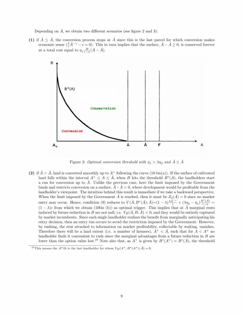
Depending on �A, we obtain two di¤erent scenarios (see �gure 2 and 3):
(1) if A � �A, the conversion process stops at A since this is the last parcel for which conversion makeseconomic sense ( �r A
� � c = 0). This in turn implies that the surface, �A� A � 0, is conserved foreverat a total cost equal to �1
Br�� (
�A� A).
Figure 2: Optimal conversion threshold with �1 > ��2 and A � �A
(2) if A > �A, land is converted smoothly up to A+ following the curve (10 bis(a)). If the surface of cultivatedland falls within the interval A+ � A � �A, when B hits the threshold B�(A), the landholders starta run for conversion up to �A. Unlike the previous case, here the limit imposed by the Governmentbinds and restricts conversion on a surface, �A�A > 0, where development would be pro�table from thelandholder�s viewpoint. The intuition behind this result is immediate if we take a backward perspective.When the limit imposed by the Government �A is reached, then it must be Z2( �A) = 0 since no marketentry may occur. Hence, condition (9) reduces to V ( �A;B�( �A); �A)=(1 � �) � �A�
r + (��2 � �1)B�( �A)r�� =
(1 � �)c from which we obtain (10bis (b)) as optimal trigger. This implies that at �A marginal rentsinduced by future reduction in B are not null, i.e. VB( �A;B; �A) < 0, and they would be entirely capturedby market incumbents. Since each single landholder realizes the bene�t from marginally anticipating hisentry decision, then an entry run occurs to avoid the restriction imposed by the Government. However,by rushing, the rent attached to information on market pro�tability, collectable by waiting, vanishes.Therefore there will be a land extent (i.e. a number of farmers), A+ < �A, such that for A < A+ nolandholder �nds it convenient to rush since the marginal advantages from a future reduction in B arelower than the option value lost.29 Note also that, as A+ is given by B�(A+) = B�( �A), the threshold
29This means the A+th is the last landholder for whom VB(A+; B�(A+); �A) = 0:
9
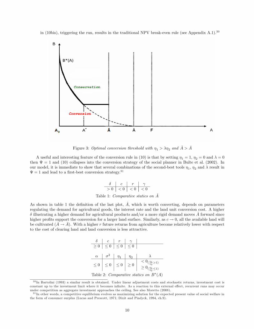
in (10bis), triggering the run, results in the traditional NPV break-even rule (see Appendix A.1).30
Figure 3: Optimal conversion threshold with �1 > ��2 and A > �A
A useful and interesting feature of the conversion rule in (10) is that by setting �1 = 1; �2 = 0 and � = 0then = 1 and (10) collapses into the conversion strategy of the social planner in Bulte et al. (2002). Inour model, it is immediate to show that several combinations of the second-best tools �1; �2 and � result in = 1 and lead to a �rst-best conversion strategy.31
� c r > 0 < 0 < 0 < 0
Table 1: Comparative statics on A
As shown in table 1 the de�nition of the last plot, A, which is worth converting, depends on parametersregulating the demand for agricultural goods, the interest rate and the land unit conversion cost. A higher� illustrating a higher demand for agricultural products and/or a more rigid demand moves A forward sincehigher pro�ts support the conversion for a larger land surface. Similarly, as c! 0, all the available land willbe cultivated (A! �A). With a higher r future returns from agriculture become relatively lower with respectto the cost of clearing land and land conversion is less attractive.
� c r � 0 � 0 � 0 � 0
� �2 �1 �2 �
� 0 � 0 � 0 � 0< 0( �1�2>1)� 0( �1�2�1)
Table 2: Comparative statics on B�(A)
30 In Bartolini (1993) a similar result is obtained. Under linear adjustment costs and stochastic returns, investment cost isconstant up to the investment limit where it becomes in�nite. As a reaction to this external e¤ect, recurrent runs may occurunder competition as aggregate investment approaches the ceiling. See also Moretto (2008).31 In other words, a competitive equilibrium evolves as maximizing solution for the expected present value of social welfare in
the form of consumer surplus (Lucas and Prescott, 1971; Dixit and Pindyck, 1994, ch.9).
10
In table 2, we provide some comparative statics illustrating the e¤ect that changes in the exogenous pa-rameters have on the threshold level B�(A). Changes in an exogenous parameter, whenever increasing(decreasing) conversion bene�ts with respect to conservation bene�ts, rede�ne, by moving upward (down-ward) the boundary B�(A), the conversion and conservation regions. In this light, for instance, to a higher� corresponds higher pro�ts from agriculture and thus a higher B�(A) and a larger conversion region. Thesame e¤ect is also produced by a relatively more inelastic demand. On the contrary, the opposite occurs asc increases since a higher conversion cost decreases net conversion bene�ts.With an increase in the interestrate, exercise of the option to convert should be anticipated but this e¤ect is too weak to prevail over thee¤ect that a higher r has on the cost opportunity of conversion. Studying the e¤ect of volatility, �, andof growth parameter, �, the sign of the derivatives is in line with the standard insight in the real optionsliterature. An increase in the growth rate and volatility of B determines postponed exercise of the optionto convert. This can be explained by the need to reduce the regret of taking an irreversible decision underuncertainty. Since the cost of this decision is growing at a faster rate and there is uncertainty about itsmagnitude, waiting to collect information about future prospects is a sensible strategy.As expected, an increase in �1 pushes the barrier downward since it makes it more pro�table to conserve
the plot and keep open the option to convert. In line with this result, the barrier responds in the oppositeway to an increase in �2 which implicitly provides an incentive to conversion. Changes in � have a non-monotonic e¤ect on the barrier which depends on the ratio between the two payment rates. A higher �de�nes a stricter requirement on development that may push the barrier downward for two reasons. First,a lower return from agriculture since less land is cultivated which is, however, balanced by a lower cost forclearing land, and second, as �1�2 > 1 a higher payment on the marginal unit which the farmer is required toset aside is guaranteed if the plot is totally conserved. The case where �1
�2� 1 and the barrier shifts upward
can be easily explained by inverting the second argument.These considerations mostly hold for both (10) and (10 bis). Clearly, over the interval A+ < A � �A since
the option multiple, �2�2�1
, drops out, the barrier B�(A) is not a¤ected by �. The derivative with respect tothe bene�t drift � maintains the sign in table 2 while the comparative statics on r reveals:
@B�(A)
@r=
(> 0 for r < �( A�A )
� 0 for r � �( A�A )
for A+ < A � �A
Finally, since by (10bis) the same level of B triggers the entry of a positive mass of landholders, i.e. B�(A+) =B�( �A), it is worth highlighting that the surface triggering a conversion rush is independent of the de�nitionof �1, �2 and �. The Government policy may either speed up or slow down the conversion dynamic butit cannot alter A+ which depends only on the choice of �A with respect to A. Note that @A+
@ �A> 0 which
reasonably means that as �A! A the run would be triggered only by a relatively a lower level for B. In otherwords, since in expected terms a higher �A implies a less strict threat of being regulated, then landholders arenot willing to give up information rents collectable by waiting. Not surprisingly, @A
+
@A< 0. A lower A implies
a faster drop in the pro�t from agriculture as A increases and then a lower incentive for the conversion run.
3.2 Case with �1 < ��2Now, assume that �1 < ��2. In this case �2 > �1 will necessarily obtain, that is, the payment rate per unit ofland conserved is more generous when a portion of the plot has been developed. This could be the case for aGovernment which, having run out of funding for the conservation program, may be willing to sacri�ce somepristine habitat in order to more generously �nance conservation on a smaller scale.32 Di¤erently, this choicemay also be reasonably explained by a Government wishing to indirectly induce a switch towards certainagricultural or forestry practises by o¤ering a more favourable payment rate. For instance, the Governmentmay choose to prefer timber harvest and subsequent reforestation as land-use to cash funding on carbonmarkets and �nance conservation on the remaining habitat.33 In this case, our model allows framing of
32Note that this scenario does not exclude to push toward a form of development which is perceived as environmental-friendly.33Under the CDM (Clean Development Mechanism) of the Kyoto Protocol, forest conservation/avoided deforestation e¤orts
were not considered in the �rst commitment period (2008-2012) (IPCC, 2007). On the contrary, through the CDM, investmentin tree planting projects has been undertaken (Santilli et al., 2005; van Vliet, 2003). In our model, this would imply an �1 lower
11
the competition between these two "green" but mutually exclusive land destinations, i.e. secondary forestsvs. primary forests. Finally, the Government could simply consider it fair and/or politically expedient tobetter reward conservation as soon as the restriction on development is binding and the real conservationcost opportunity is implicitly revealed.As in the previous section, the optimal conversion threshold, BC(A) = B��(A), must be determined by
matching bene�ts and costs from conversion. Unlike the previous case, when developing land in addition tothe pro�t accruing from agriculture, (1��) �A�
r , the landholder can earn a higher payment for ES provisionsince (��2 � �1) B
r�� > 0. Hence, it makes sense to clear land as B increases. However, as above marketcompetition has a negative e¤ect on the value from farming which, being entry-free, lies below (1��)c. Thise¤ect is accounted for the �rst term (Z1(A) � 0 for A � �A) in (7) since as limB!0 V (A;B; �A) = 0 then tokeep V (A;B; �A) �nite we must set Z2 = 0. It follows that (7) reduces to:
V (A;B; �A) = Z1(A)B�1 + (1� �)�
rA� + (��2 � �1)
B
r � � (11)
As in the previous case, we determine Z1(A) and B��(A) by imposing the free entry condition and zeromarginal rents at B��(A). That is,
Proposition 2 Provided that each agent rationally forecasts the future dynamics of the market for agricul-tural goods for land to be converted the following condition must hold
V (A;B��(A); �A) = (1� �)c (12)
where the conversion rule is
(i) if A � �A then
B��(A) =
8>><>>:0; for A0 < A � A (a)�1�1�1
(r � �) h1� ( AA )
ic; for A < A � A++ (b)
(r � �)h1� ( A�A )
ic; for A++ < A � �A; (c)
(13)
(ii) if A > �A thenB��(A) = 0; for A0 < A � �A (13 bis)
where = 1����2��1
; A = ( �rc )1= and A++ = [ (�1�1)
�A� +A�
�1]�
1 .
Proof. See appendix A.3.Equation (12) de�nes the dynamic zero pro�t condition which must hold at B��(A). Proposition 2
illustrates the conversion dynamic as B �uctuates according to (2). Here, unlike the previous case, thethreshold B��(A) is an increasing continuous function of A and the conversion region is above the barrier.Development is worthwhile only if B crosses B��(A) from below. In the conservation region the landholderconserves as B is not high enough to trigger conversion and waits until the stochastic process B moves upto B��(A). At that point, a mass of landholders enters the market keeping pro�ts low enough to push thebarrier upward.
than �2 in relative terms. Only recently, at the December 2009 United Nations Framework Convention on Climate Change(UNFCCC) meeting in Copenhagen this controversial issue discussed and �nally forest conservation should now be allowed toqualify (Phelps et al., 2010). See also Fargione et al. (2008) on land clearing and biofuel carbon debt. On palm oil trees vs.primary forests see Butler et al., (2009), Fitzherber et al., (2008) and Koh and Ghazoul (2008).
12
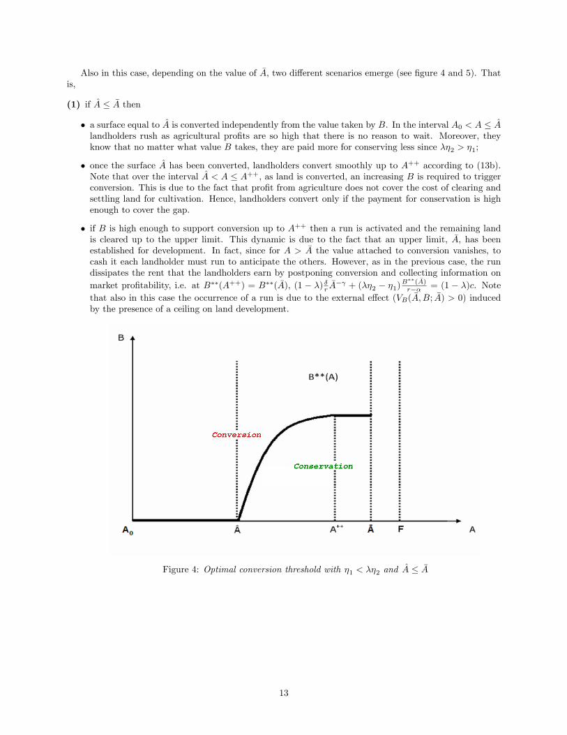
Also in this case, depending on the value of �A, two di¤erent scenarios emerge (see �gure 4 and 5). Thatis,
(1) if A � �A then
� a surface equal to A is converted independently from the value taken by B. In the interval A0 < A � Alandholders rush as agricultural pro�ts are so high that there is no reason to wait. Moreover, theyknow that no matter what value B takes, they are paid more for conserving less since ��2 > �1;
� once the surface A has been converted, landholders convert smoothly up to A++ according to (13b).Note that over the interval A < A � A++, as land is converted, an increasing B is required to triggerconversion. This is due to the fact that pro�t from agriculture does not cover the cost of clearing andsettling land for cultivation. Hence, landholders convert only if the payment for conservation is highenough to cover the gap.
� if B is high enough to support conversion up to A++ then a run is activated and the remaining landis cleared up to the upper limit. This dynamic is due to the fact that an upper limit, �A, has beenestablished for development. In fact, since for A > �A the value attached to conversion vanishes, tocash it each landholder must run to anticipate the others. However, as in the previous case, the rundissipates the rent that the landholders earn by postponing conversion and collecting information onmarket pro�tability, i.e. at B��(A++) = B��( �A), (1 � �) �r �A
� + (��2 � �1)B��( �A)r�� = (1 � �)c. Note
that also in this case the occurrence of a run is due to the external e¤ect (VB( �A;B; �A) > 0) inducedby the presence of a ceiling on land development.
Figure 4: Optimal conversion threshold with �1 < ��2 and A � �A
13
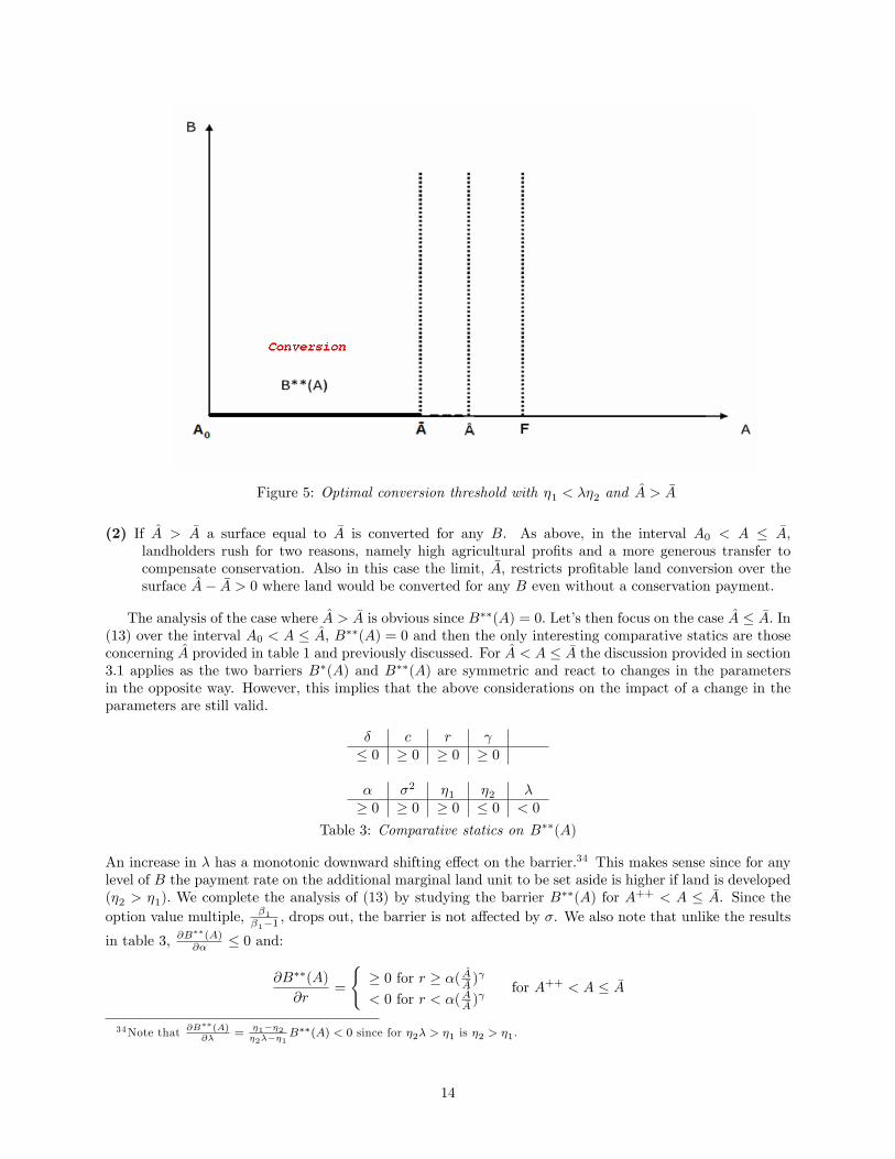
Figure 5: Optimal conversion threshold with �1 < ��2 and A > �A
(2) If A > �A a surface equal to �A is converted for any B. As above, in the interval A0 < A � �A,landholders rush for two reasons, namely high agricultural pro�ts and a more generous transfer tocompensate conservation. Also in this case the limit, �A, restricts pro�table land conversion over thesurface A� �A > 0 where land would be converted for any B even without a conservation payment.
The analysis of the case where A > �A is obvious since B��(A) = 0. Let�s then focus on the case A � �A. In(13) over the interval A0 < A � A, B��(A) = 0 and then the only interesting comparative statics are thoseconcerning A provided in table 1 and previously discussed. For A < A � �A the discussion provided in section3.1 applies as the two barriers B�(A) and B��(A) are symmetric and react to changes in the parametersin the opposite way. However, this implies that the above considerations on the impact of a change in theparameters are still valid.
� c r � 0 � 0 � 0 � 0
� �2 �1 �2 �� 0 � 0 � 0 � 0 < 0
Table 3: Comparative statics on B��(A)
An increase in � has a monotonic downward shifting e¤ect on the barrier.34 This makes sense since for anylevel of B the payment rate on the additional marginal land unit to be set aside is higher if land is developed(�2 > �1). We complete the analysis of (13) by studying the barrier B
��(A) for A++ < A � �A. Since theoption value multiple, �1
�1�1, drops out, the barrier is not a¤ected by �. We also note that unlike the results
in table 3, @B��(A)@� � 0 and:
@B��(A)
@r=
(� 0 for r � �( A�A )
< 0 for r < �( A�A )
for A++ < A � �A
34Note that @B��(A)@�
=�1��2�2���1
B��(A) < 0 since for �2� > �1 is �2 > �1:
14
Finally, also in this case, the policy parameters �1, �2 and � are neutral in the de�nition of A++ in (13 bis).
This threshold depends only on A and the ceiling �A. We �nd that @A++
@ �A> 0 and @A++
@A> 0. If the limit �A
is less strict, the landholders are less willing to dissipate information rents and participate in the run onlyfor high level of B. A lower A implies a faster fall in the pro�t from agriculture as A increases and then ahigher incentive for developing land as soon as B is high enough. Since this consideration is anticipated byall landholders, the run starts at a lower A++.
4 Voluntary participation or contract enforceability?
Once the optimal conversion rules have been determined, we focus in this section on the issue of voluntaryparticipation which is a crucial aspect in a PES scheme (Wunder, 2005). In this section we present the con-ditions under which the conservation contract is accepted on a voluntary basis. In this respect, two elementsmust be considered. First, the dynamic of the whole conversion process involving all the landholders whoenrolled under the conservation program. Second, the restrictions on land development that the Governmentmay wish to impose in the form of takings on landholders not entering the conservation program.35
Focusing on the second element, the Government may �nd it desirable for the landholder to only partiallydevelop his plot, i.e. 0 < � � 1. Conversely, from (9) and (12) it emerges that the landholder may considerit pro�table to develop the entire plot, i.e. � = 0. Therefore, the conservation contract may be accepted on avoluntary basis only if each landholder is better-o¤ signing it than not. As can be easily seen, the acceptancewill depend on the expectation concerning the ability of the Government to impose a � > 0. Let�s formalizethis consideration assuming that no compensation is paid if a taking occurs. Since by propositions 1 and 2the conversion is optimal at BC(A) with C =�;��, then an in�nitely living landholder signs the contract ifand only if:
�1r � �B
C(A) + V (A;BC(A); �A) � Et�Z 1
t
e�r(s�t)(1� ��)�A(s)� ds�
for C =�;�� (14)
where � 2 [0; 1] is the probability of regulation, i.e. the restriction � holds also for landholders not signingthe contract. In (14) the LHS describes the position of a landholder within the program while on the RHSwe have the expected present value for a landholder not accepting the contract and developing land at timet. Note that in the last case the conversion option is exercised as soon as the expected cost of conversion,(1� ��)c, equals the expected bene�t from conversion. Rearranging (14) yields:
�1r � �B
C(A) + (1� �)c � (1� ��)c (15)
which holds if�1B
C(A)� �(1� �)(r � �)c � 0 for C =�;��
where (r��)c is the annualized conversion cost. Depending on the parameters this condition may not holdfor some A. Note in fact that since B�(A) is a decreasing function of A, while B��(A) is increasing, (15)implies that:
Proposition 3 If � 2 [0; 1) then contract acceptance can be voluntary for some but not all the landholdersin the conservation program.
Proof. Straightforward from propositions 1 and 2.Segerson and Miceli (1998) show that an agreement can always be signed on a voluntary basis if the
probability of future regulation is positive. By Proposition 3 we show that this result does not hold in ourframe. In fact, uncertainty about future regulation does not allow capturing of all the agents who can be
35Although most of the PES programs in developing countries were introduced as quid pro quo for legal restrictions on landclearing, there are no speci�c contract conditions preventing the landholder from clearing the area enrolled under the program(Pagiola, 2008, p. 717). In principle, sanctions may apply. For instance, in the PSA (Pagos por Servicios Ambientales) programin Costa Rica, payments received plus interest should be returned by the landholders exiting the scheme (FONAFIFO, 2007).However, in a developing country context, economic and political costs may reduce the enforcement of such sanction.
15
potentially regulated. A similar result is obtained by Langpap and Wu (2004) in a regulator-landowner two-period model for conservation decisions under uncertainty and irreversibility. In their paper, since contractpay-o¤s are uncertain and signing is an irreversible decision, under certain conditions a landholder may notaccept it to stay �exible. Unlike them, we show that under the same threat of regulation a contract can bevoluntarily signed by some landholders and not by others. Not surprisingly, imposing by contract constraintson land development reduces �exibility and discourages voluntary participation. Clearly, due to decreasingpro�t from agriculture, this holds for some landholders but not for all since entering the conservation programbecomes more attractive as land is progressively cleared.36
Summing up, we can conclude that voluntary participation crucially depends on the likelihood of takingsbut also on the magnitude of the compensation payment which a court may impose. In fact, needless tosay, if takings can be compensated, then, by (14) and (15), the requirement for contract acceptance becomesmore stringent and it is more di¢ cult to sustain agreements on a voluntary basis.37
5 The long-run average rate of forest conversion
In line with Ferraro (2001, p. 997) we have shown that even if the ES provided by a targeted ecosystem (�1 �1) is not entirely compensated for, we may be able to induce landholders to conserve their plot. However,we believe that this result only "statically" addresses the conservation/development dilemma. Hence, in thissection we aim to study the temporal implications of the optimal conversion policy, i.e. how long it takes toclear the target surface �A, and the impact of increasing uncertainty about future environmental bene�ts, B,and conversion cost, c, on conversion speed under the two policy scenarios characterized above. To do so,we derive the long-run average growth rate of forest conversion through a robust linear approximation (seeAppendix A.4 and A.5).38
5.1 Case with �1 > ��2Let�s consider the case where bA � �A. This represents the more interesting case since the analysis belowremains valid also for the opposite case over the range A < A+. Note in fact that for A � A+ the long-runrate of reforestation must obviously tend to in�nity due to the conversion run.Let�s now focus our attention on the long-run average growth rate of forest conversion. Rearranging (10)
yields:
�=�2
�2 � 1(1� �) PA (A)
r� �1 � ��2
r � � B for � < � (16)
where �= �2�2�1
(1� �) c.The �rst term on the RHS of (16) represents the expected discounted pro�t from the cultivation of land
conditional on the number of farmers remaining constant. The multiple �2�2�1
< 1 accounts for the presenceof uncertainty and irreversibility. The second term is the expected discounted �ow of payments implicitlygiven up by developing land net of the payments for conservation paid for setting aside � as required bythe Government. Note that � can be de�ned as a regulated process in the sense of Harrison (1985, chp. 2)with � as upper re�ecting barrier. This implies that when a reduction of B drives � upward toward � somelandholders �nd it pro�table to convert land. New entries in the market, however, determine a drop alongPA (A) which by balancing for the e¤ect of B prevents � from rising above �. Since entry is instantaneous,the rate of deforestation is in�nite at �.39 Conversely, if � < � the level of B is high enough to supportconservation, no entries occur and consequently the deforestation rate is null. Hence, the re�ecting barrier
36Note that in this respect the scenario �1 < ��2 is the most problematic since switching to competitive farming is soadvantageous for the �rst developers that they never accept the contract. This implies that (1) should be restated as L0 = A00+Fwith A00 > A0 since by (15) only a lower number of landholders may enter the program on a voluntary basis.37On compensation and land taking see Adler (2008).38See Dixit and Pindyck (1994, pp. 372-373), and Hartman and Hendrickson (2002) for a calculation of the long-run average
growth rate of investment.39The fact that at � the rate of conversion is in�nite follows from the non-di¤erentiability of B and then of A with respect to
the time t (see Harrison, 1985; Dixit, 1993).
16
� does not generate a �nite rate of deforestation over time but long periods of inaction followed by shortperiods of rapid bursts of land conversion.In this section, our aim is to then �nd a steady-state (long-run) distribution for A from which we
can determine the average growth rate of forest conversion over a long period of time. Since A and Benter additively on (16) some manipulation is required to apply the well-known properties of log-normaldistribution and show that � is log-normally distributed.40 Denoting by 1
dtE(d lnA) the measure of theaverage growth rate of forest conversion, in the appendix we prove that:
Proposition 4 When �1 > ��2, for an initial point ( ~B; ~A) such that �( ~B; ~A) = � (10) can be approximatedby
A~A= (
BeB )� 1
h1�( ~A
A) i
(17a)
and the average or expected long-run growth rate of deforestation can be approximated by:
1
dtE [d lnA] ' �
�� 12�
2
[1� (
~A
A) ] for � <
1
2�2 (17b)
where A0 � ~A < A and A = ( �rc )1= .
Proof. See Appendix A.5.Thus, if ~B is the current value of ES and, by (10), ~A is the corresponding optimal surface of converted
land, the expression in (17b) is the best guess for the average rate at which the forested surface, �A � ~A, iscleared. Remember that if then ~A > A the deforestation rate is null since �
rA� < c for bA < A � A.
Furthermore, it is straightforward to verify that the rate in (17b) is increasing in the volatility of futurepayments. Although at a �rst glance this result may seem counterintuitive, it follows from the distributionof the log-normal process � with an upper re�ecting barrier at �. A higher volatility has two distinct e¤ects.First, it pushes the barrier � downward; second, by increasing the positive skewness of the distribution of �,it raises the probability of the barrier being reached.41 Both e¤ects induce a higher rate of deforestation inboth the short-run and long-run.We also note that a higher conversion cost c induces a lower long-run average rate of deforestation. Two
e¤ects must be recognized. The �rst is immediate and driven by the higher c. The second is more subtle. Ahigher c prevents from converting now for a certain B. Since conversion in the future will be triggered by adecreasing B the landholder can bene�t from an implicit advantage by paying a lower (�1 � ��2)B which isa conversion cost opportunity.
5.2 Case with �1 < ��2Consider the interval bA � �A.42 Rearranging (13) yields:
& =�1
�1 � 1(1� �) PA(A)
r+��2 � �1r � � B for & < & (18)
where & = �1�1�1
(1� �) c.The �rst term on the RHS of (18) is the expected discounted pro�t from the cultivation of land if any
further conversion occurs. The multiple �1�1�1
> 1 accounts for uncertainty and irreversibility. Unlike (16),since �1 < ��2 the second term stands for the expected discounted �ow of payments received when developing�; net of the payments implicitly given up. Again, & can be characterized as a regulated process having & asupper re�ecting barrier. Whenever an increase in B leads & upward toward & new plots are cleared. This willproduce an increase in the supply of agricultural goods and consequently a drop along PA (A) preventing &from passing &. It follows that to keep the surface conserved unchanged, we must have & > &.
40Technically, the log-normality is a property of the process for � linearized around an initial point ( ~B; ~A). See Appendix A.5for further details.41We show in appendix A.6 that to a higher � corresponds a higher probability of hitting � and thus a higher long run average
deforestation rate.42The same discussion provided in the previous section applies for A � A++.
17
As shown in the appendix:
Proposition 5 When �1 > ��2, for an initial point ( ~B; ~A) such that &( ~B; ~A) = & (13) can be approximatedby:
A~A= (
BeB )� 1
h1�( ~A
A) i
(19a)
and the average or expected long-run growth rate of deforestation can be approximated by:
1
dtE [d lnA] '
�� 12�
2
[(~A
A) � 1] for � >
1
2�2 (19b)
where ~A > A and A = ( �rc )1= .
Proof. See Appendix A.5.As above, (19b) is the best guess for the average rate at which the forest stock, �A� ~A, is exhausted over a
long-run horizon. Furthermore, the long-run average rate of deforestation (19b) is decreasing in the volatilityof future payments. Again, it should be remembered that & is a log-normal process with an upper re�ectingbarrier at &. As volatility soars the barrier & moves upward and positive skewness in the distribution of &increases. Whilst the �rst has a reducing e¤ect on the rate, the second raises the probability of hitting & andconsequently the rate of deforestation.43 In addition, since the expected discounted pro�t from competitivefarming decreases as land is converted, the former e¤ect prevails in the long-run. Conversely, we �nd thatthe rate is increasing in c. This may seem surprising at �rst sight. As a higher c prevents conversion wewould expect landholders to hold on the decision to develop, but postponing conversion is costly since theper-period increase in payments (��2 � �1)B > 0 would have to be given up. Since the weight of expecteddiscounted higher payments accruing if conversion is anticipated prevails over the expected pay-o¤ fromdelay, the average rate of deforestation is increasing in c. More formally, a higher c, by inducing a shiftupward for the barrier, should de�nitely decrease the probability of hitting it. However, as c increases, thenA decreases and so does A++. This means that a run will start at a lower surface A++ as soon as B��( �A)has been reached. Since the run will exhaust the stock �A and drastically lower the pro�t from agriculture
then A++ � A landholders will prefer to anticipate the conversion. Note that since @(A++�A)@A
> 0 , even fora B < B��( �A), they will prefer to convert to trade-o¤ the dramatic e¤ect on the pro�t due to the run witha higher pro�t from farming. This latter e¤ect justi�es a higher deforestation rate in the long-run.
6 The Costa Rica case study
In this section we provide a numerical example to illustrate our �ndings. We calibrate the model to �t thecharacteristics of a humid Atlantic zone of Costa Rica.44 Parameters in our calculations take the followingvalues:
1. The total extent of originally forested area is �A = 320000 hectares. On this extent, we consider aconverted portion equal to A0 = 25000 hectares.45 We draw demand for agricultural products as inBulte et al. (2002) by setting � = $6990062 (in 1998 US$) and = 0:887.
2. The annual value of ES is equal to ~B = $75=ha. This value accounts only for the forest productionfunction and does not include the regulatory function and existence values. As B is assumed to �uctuateaccording to (2) we investigate the impact of its drift, �, and volatility, �, on the optimal forest stock.To do this, in our analysis � takes values 0, 0:025, and 0:05 while � varies within the interval [0; 0:325].
3. A 7% risk free interest rate is assumed (r = 0:07). Finally, unlike Bulte et al. (2002) where c = 0 wealso consider di¤erent levels of costly deforestation.
43See appendix A.6 for the intuition behind this result.44Detailed data are provided by Bulte et al. (2002, pp. 154-155). See also Conrad (1997).45Note that later we will set ~A = A0 = 25000.
18
6.1 Optimal forest stock and long-run average rate of deforestation under dif-ferent payment schemes
6.1.1 Case with �1 > ��2
For the case �1 > ��2 we study the following �ve di¤erent policy scenarios:
�1 �2 � Scenario 1 1 0 0 1Scenario 2 0:7 0 0 1:4286Scenario 3 1 0 0:3 0:7Scenario 4 0:7 0:5 0:3 1:2727Scenario 5 0:7 1 0:3 1:75
Table 4: policy scenarios
and compare them for two di¤erent levels of costly deforestation, c = 0 and c = 500, respectively.46 Inparticular, by these comparisons, our aim is
- 1 vs. 2: to highlight the impact of a reduction in the compensation for ES provision on the landholders�decision to conserve. Note that scenario 1 resembles the case of a centralized economy in Bulte etal. (2002) where the planner optimally allocates land by comparing expected marginal bene�t fromconservation and its expected marginal cost opportunity.
- 1 vs. 3: to study the e¤ect of restricted land development on the optimal forest stock and on the long-runaverage rate of deforestation.
- 4 vs. 5: to verify the e¤ect of a more favourable conservation payment rate when the restriction on landdevelopment is binding (i.e. land development is privately optimal).
In the tables below we provide the optimal forest stock which should be held, �A� ~A,47 and the averagedeforestation rate (Def rate) at which such stock should be optimally exhausted in the long-run.48 Notethat in our calculations the deforestation rate may be null in two cases. First, when the optimal foreststock, �A � ~A is completely exhausted and second, when conditions in (17b) or (19b) do not hold. We willdistinguish between them using 0 for the former and a dash for the latter.
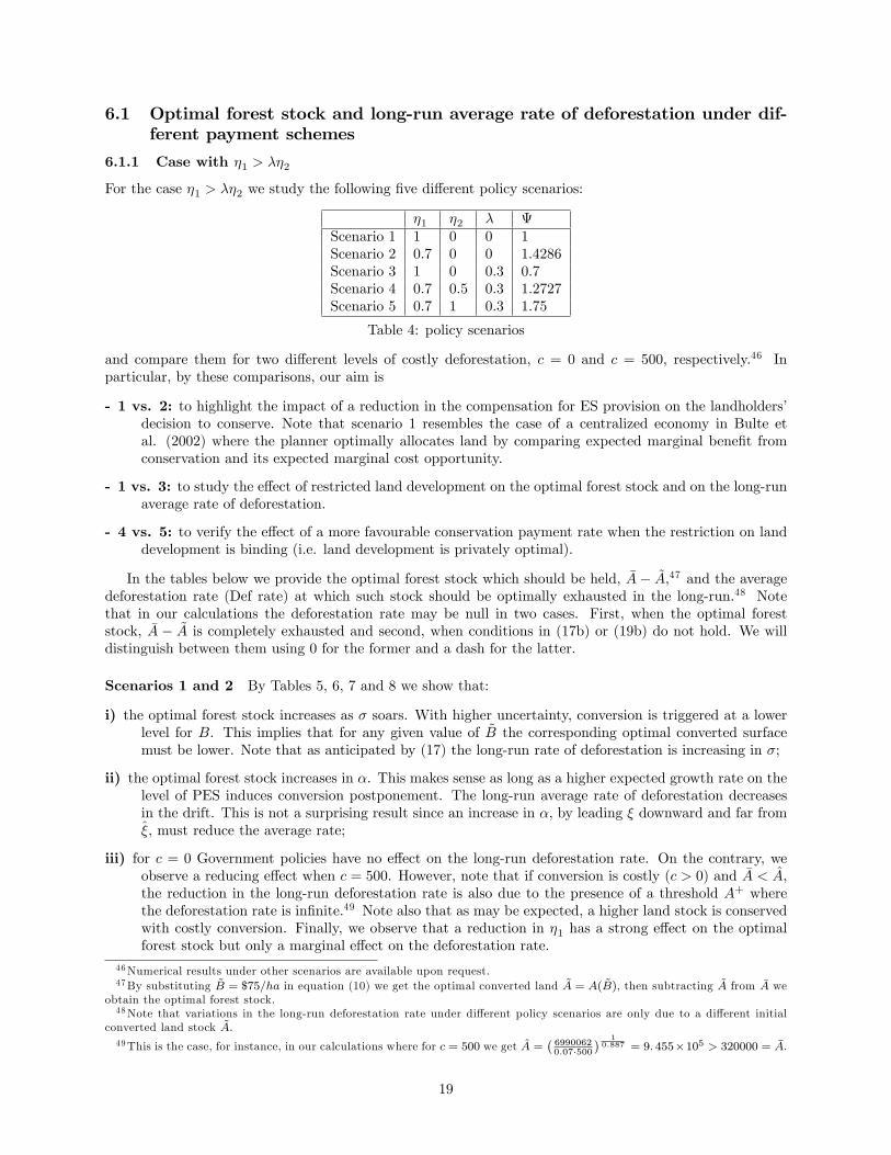
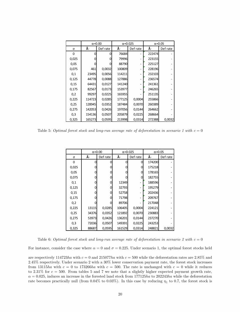
Scenarios 1 and 2 By Tables 5, 6, 7 and 8 we show that:
i) the optimal forest stock increases as � soars. With higher uncertainty, conversion is triggered at a lowerlevel for B. This implies that for any given value of ~B the corresponding optimal converted surfacemust be lower. Note that as anticipated by (17) the long-run rate of deforestation is increasing in �;
ii) the optimal forest stock increases in �. This makes sense as long as a higher expected growth rate on thelevel of PES induces conversion postponement. The long-run average rate of deforestation decreasesin the drift. This is not a surprising result since an increase in �, by leading � downward and far from�, must reduce the average rate;
iii) for c = 0 Government policies have no e¤ect on the long-run deforestation rate. On the contrary, weobserve a reducing e¤ect when c = 500. However, note that if conversion is costly (c > 0) and �A < A,the reduction in the long-run deforestation rate is also due to the presence of a threshold A+ wherethe deforestation rate is in�nite.49 Note also that as may be expected, a higher land stock is conservedwith costly conversion. Finally, we observe that a reduction in �1 has a strong e¤ect on the optimalforest stock but only a marginal e¤ect on the deforestation rate.
46Numerical results under other scenarios are available upon request.47By substituting ~B = $75=ha in equation (10) we get the optimal converted land ~A = A( ~B), then subtracting ~A from �A we
obtain the optimal forest stock.48Note that variations in the long-run deforestation rate under di¤erent policy scenarios are only due to a di¤erent initial
converted land stock ~A:
49This is the case, for instance, in our calculations where for c = 500 we get A =�69900620:07�500
� 10:887 = 9: 455�105 > 320000 = �A.
19
σ ĀÃ Def rate ĀÃ Def rate ĀÃ Def rate0 0 0 76684 222474
0,025 0 0 79996 223155 0,05 0 0 88790 225127 0,075 461 0,0032 100809 228196
0,1 23495 0,0056 114211 232103 0,125 44778 0,0088 127886 236574 0,15 64431 0,0127 141240 241361 0,175 82567 0,0173 153977 246265
0,2 99297 0,0225 165955 251135 0,225 114723 0,0285 177125 0,0004 255866 0,25 128945 0,0352 187484 0,0070 260389 0,275 142053 0,0426 197056 0,0144 264662
0,3 154136 0,0507 205879 0,0225 268664 0,325 165273 0,0595 213998 0,0314 272388 0,0032
α=0.05α=0.025α=0.00
Table 5: Optimal forest stock and long-run average rate of deforestation in scenario 1 with c = 0
σ ĀÃ Def rate ĀÃ Def rate ĀÃ Def rate0 0 0 0 0 174200
0,025 0 0 0 0 175218 0,05 0 0 0 0 178165 0,075 0 0 0 0 182755
0,1 0 0 12349 188596 0,125 0 0 32793 195279 0,15 0 0 52758 202436 0,175 0 0 71798 209767
0,2 0 0 89706 217048 0,225 13115 0,0285 106405 0,0004 224121 0,25 34376 0,0352 121892 0,0070 230883 0,275 53973 0,0426 136201 0,0144 237270
0,3 72036 0,0507 149391 0,0225 243253 0,325 88687 0,0595 161529 0,0314 248821 0,0032
α=0.00 α=0.025 α=0.05
Table 6: Optimal forest stock and long-run average rate of deforestation in scenario 2 with c = 0
For instance, consider the case where � = 0 and � = 0:225. Under scenario 1, the optimal forest stocks held
are respectively 114723ha with c = 0 and 215077ha with c = 500 while the deforestation rates are 2:85% and2:45% respectively. Under scenario 2 with a 30% lower conservation payment rate, the forest stock increasesfrom 13115ha with c = 0 to 173266ha with c = 500. The rate is unchanged with c = 0 while it reducesto 2:31% for c = 500. From tables 5 and 7 we note that a slightly higher expected payment growth rate,� = 0:025, induces an increase in the forested land stock from 177125ha to 202243ha while the deforestationrate becomes practically null (from 0:04% to 0:03%). In this case by reducing �1 to 0:7, the forest stock is
20
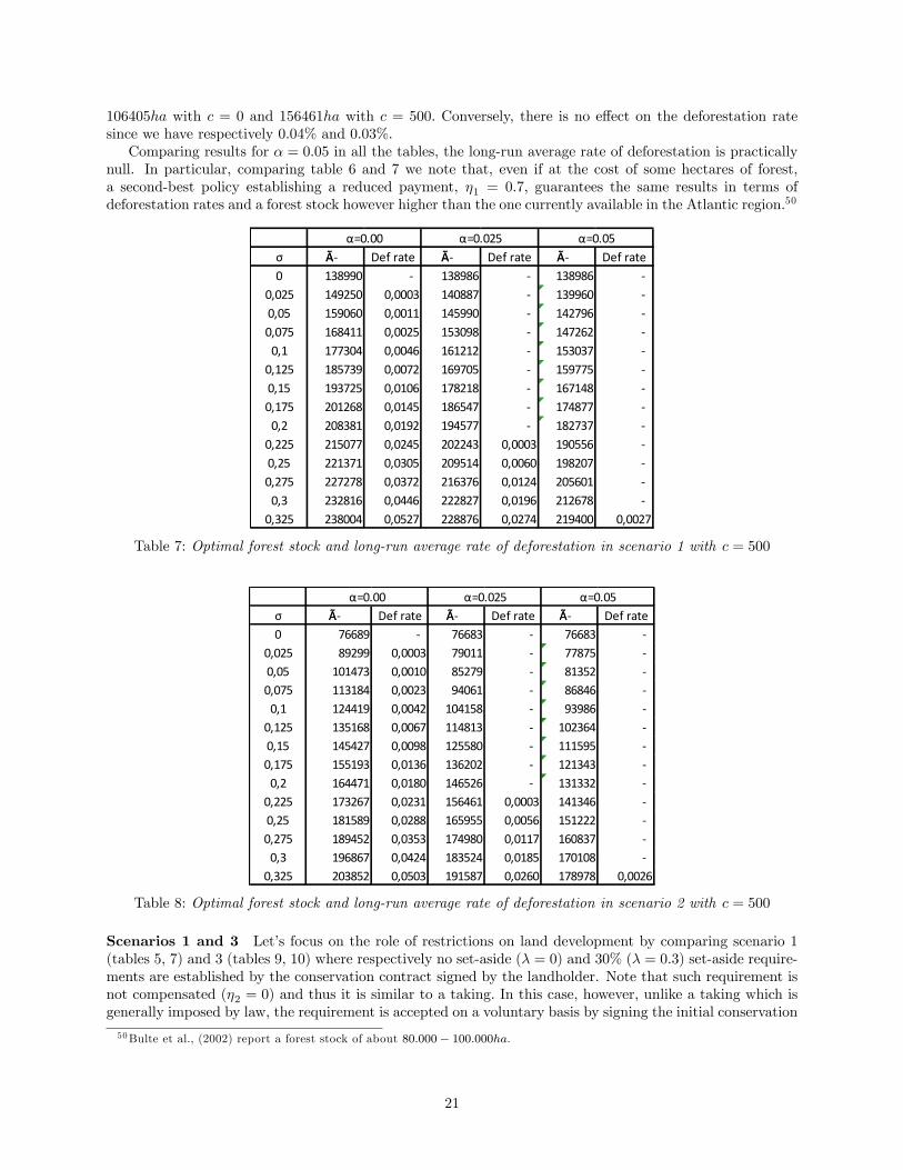
106405ha with c = 0 and 156461ha with c = 500. Conversely, there is no e¤ect on the deforestation ratesince we have respectively 0:04% and 0:03%.Comparing results for � = 0:05 in all the tables, the long-run average rate of deforestation is practically
null. In particular, comparing table 6 and 7 we note that, even if at the cost of some hectares of forest,a second-best policy establishing a reduced payment, �1 = 0:7, guarantees the same results in terms ofdeforestation rates and a forest stock however higher than the one currently available in the Atlantic region.50
σ ĀÃ Def rate ĀÃ Def rate ĀÃ Def rate0 138990 138986 138986
0,025 149250 0,0003 140887 139960 0,05 159060 0,0011 145990 142796 0,075 168411 0,0025 153098 147262
0,1 177304 0,0046 161212 153037 0,125 185739 0,0072 169705 159775 0,15 193725 0,0106 178218 167148 0,175 201268 0,0145 186547 174877
0,2 208381 0,0192 194577 182737 0,225 215077 0,0245 202243 0,0003 190556 0,25 221371 0,0305 209514 0,0060 198207 0,275 227278 0,0372 216376 0,0124 205601
0,3 232816 0,0446 222827 0,0196 212678 0,325 238004 0,0527 228876 0,0274 219400 0,0027
α=0.05α=0.025α=0.00
Table 7: Optimal forest stock and long-run average rate of deforestation in scenario 1 with c = 500
σ ĀÃ Def rate ĀÃ Def rate ĀÃ Def rate0 76689 76683 76683
0,025 89299 0,0003 79011 77875 0,05 101473 0,0010 85279 81352 0,075 113184 0,0023 94061 86846
0,1 124419 0,0042 104158 93986 0,125 135168 0,0067 114813 102364 0,15 145427 0,0098 125580 111595 0,175 155193 0,0136 136202 121343
0,2 164471 0,0180 146526 131332 0,225 173267 0,0231 156461 0,0003 141346 0,25 181589 0,0288 165955 0,0056 151222 0,275 189452 0,0353 174980 0,0117 160837
0,3 196867 0,0424 183524 0,0185 170108 0,325 203852 0,0503 191587 0,0260 178978 0,0026
α=0.00 α=0.025 α=0.05
Table 8: Optimal forest stock and long-run average rate of deforestation in scenario 2 with c = 500
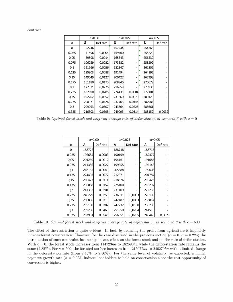
Scenarios 1 and 3 Let�s focus on the role of restrictions on land development by comparing scenario 1(tables 5, 7) and 3 (tables 9, 10) where respectively no set-aside (� = 0) and 30% (� = 0:3) set-aside require-ments are established by the conservation contract signed by the landholder. Note that such requirement isnot compensated (�2 = 0) and thus it is similar to a taking. In this case, however, unlike a taking which isgenerally imposed by law, the requirement is accepted on a voluntary basis by signing the initial conservation
50Bulte et al., (2002) report a forest stock of about 80:000� 100:000ha.
21
contract.
σ ĀÃ Def rate ĀÃ Def rate ĀÃ Def rate0 52246 157244 254765
0,025 71596 0,0004 159460 255220 0,05 89598 0,0014 165343 256539 0,075 106259 0,0032 173382 258592
0,1 121666 0,0056 182347 261206 0,125 135903 0,0088 191494 264196 0,15 149049 0,0127 200427 267398 0,175 161180 0,0173 208946 270679
0,2 172371 0,0225 216959 273936 0,225 182690 0,0285 224431 0,0004 277101 0,25 192202 0,0352 231360 0,0070 280126 0,275 200971 0,0426 237763 0,0144 282984
0,3 209053 0,0507 243664 0,0225 285661 0,325 216503 0,0595 249095 0,0314 288152 0,0032
α=0.00 α=0.025 α=0.05
Table 9: Optimal forest stock and long-run average rate of deforestation in scenario 3 with c = 0
σ ĀÃ Def rate ĀÃ Def rate ĀÃ Def rate0 188722 188718 188718
0,025 196684 0,0003 190199 189477 0,05 204239 0,0012 194161 191683 0,075 211386 0,0027 199655 195146
0,1 218135 0,0049 205888 199608 0,125 224493 0,0077 212371 204787 0,15 230473 0,0111 218826 210423 0,175 236088 0,0152 225100 216297
0,2 241352 0,0201 231109 222235 0,225 246279 0,0256 236811 0,0003 228105 0,25 250886 0,0318 242187 0,0063 233814 0,275 255190 0,0387 247232 0,0130 239298
0,3 259206 0,0463 251950 0,0204 244516 0,325 262951 0,0546 256351 0,0285 249446 0,0029
α=0.00 α=0.025 α=0.05
Table 10: Optimal forest stock and long-run average rate of deforestation in scenario 3 with c = 500
The e¤ect of the restriction is quite evident. In fact, by reducing the pro�t from agriculture it implicitlyinduces forest conservation. However, for the case discussed in the previous section (� = 0, � = 0:225) theintroduction of such constraint has no signi�cant e¤ect on the forest stock and on the rate of deforestation.With c = 0, the forest stock increases from 114723ha to 182690ha while the deforestation rate remains thesame (2:85%). For c = 500, the forested surface increases from 215077ha to 246279ha with a limited changein the deforestation rate (from 2:45% to 2:56%). For the same level of volatility, as expected, a higherpayment growth rate (� = 0:025) induces landholders to hold on conservation since the cost opportunity ofconversion is higher.
22
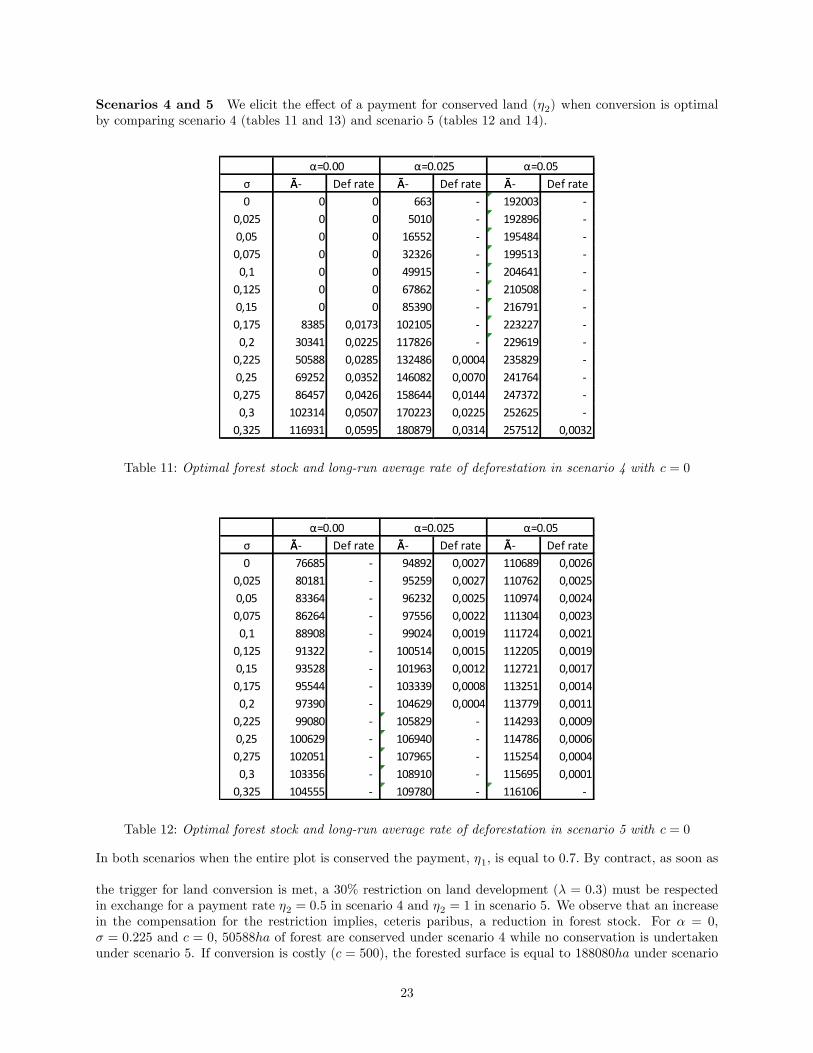
Scenarios 4 and 5 We elicit the e¤ect of a payment for conserved land (�2) when conversion is optimalby comparing scenario 4 (tables 11 and 13) and scenario 5 (tables 12 and 14).
σ ĀÃ Def rate ĀÃ Def rate ĀÃ Def rate0 0 0 663 192003
0,025 0 0 5010 192896 0,05 0 0 16552 195484 0,075 0 0 32326 199513
0,1 0 0 49915 204641 0,125 0 0 67862 210508 0,15 0 0 85390 216791 0,175 8385 0,0173 102105 223227
0,2 30341 0,0225 117826 229619 0,225 50588 0,0285 132486 0,0004 235829 0,25 69252 0,0352 146082 0,0070 241764 0,275 86457 0,0426 158644 0,0144 247372
0,3 102314 0,0507 170223 0,0225 252625 0,325 116931 0,0595 180879 0,0314 257512 0,0032
α=0.00 α=0.025 α=0.05
Table 11: Optimal forest stock and long-run average rate of deforestation in scenario 4 with c = 0
σ ĀÃ Def rate ĀÃ Def rate ĀÃ Def rate0 76685 94892 0,0027 110689 0,0026
0,025 80181 95259 0,0027 110762 0,00250,05 83364 96232 0,0025 110974 0,00240,075 86264 97556 0,0022 111304 0,0023
0,1 88908 99024 0,0019 111724 0,00210,125 91322 100514 0,0015 112205 0,00190,15 93528 101963 0,0012 112721 0,00170,175 95544 103339 0,0008 113251 0,0014
0,2 97390 104629 0,0004 113779 0,00110,225 99080 105829 114293 0,00090,25 100629 106940 114786 0,00060,275 102051 107965 115254 0,0004
0,3 103356 108910 115695 0,00010,325 104555 109780 116106
α=0.00 α=0.025 α=0.05
Table 12: Optimal forest stock and long-run average rate of deforestation in scenario 5 with c = 0
In both scenarios when the entire plot is conserved the payment, �1, is equal to 0:7. By contract, as soon as
the trigger for land conversion is met, a 30% restriction on land development (� = 0:3) must be respectedin exchange for a payment rate �2 = 0:5 in scenario 4 and �2 = 1 in scenario 5. We observe that an increasein the compensation for the restriction implies, ceteris paribus, a reduction in forest stock. For � = 0,� = 0:225 and c = 0, 50588ha of forest are conserved under scenario 4 while no conservation is undertakenunder scenario 5. If conversion is costly (c = 500), the forested surface is equal to 188080ha under scenario
23
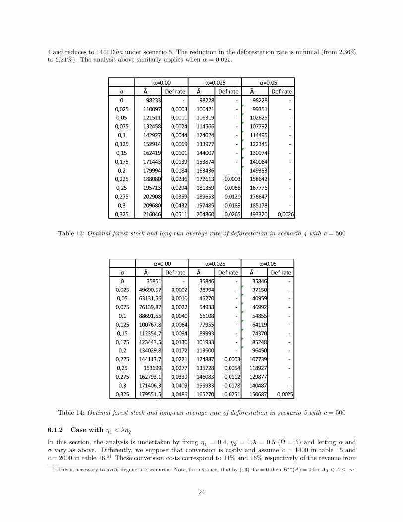
4 and reduces to 144113ha under scenario 5. The reduction in the deforestation rate is minimal (from 2:36%to 2:21%). The analysis above similarly applies when � = 0:025.
σ ĀÃ Def rate ĀÃ Def rate ĀÃ Def rate0 98233 98228 98228
0,025 110097 0,0003 100421 99351 0,05 121511 0,0011 106319 102625 0,075 132458 0,0024 114566 107792
0,1 142927 0,0044 124024 114495 0,125 152914 0,0069 133977 122345 0,15 162419 0,0101 144007 130974 0,175 171443 0,0139 153874 140064
0,2 179994 0,0184 163436 149353 0,225 188080 0,0236 172613 0,0003 158642 0,25 195713 0,0294 181359 0,0058 167776 0,275 202908 0,0359 189653 0,0120 176647
0,3 209680 0,0432 197485 0,0189 185178 0,325 216046 0,0511 204860 0,0265 193320 0,0026
α=0.00 α=0.025 α=0.05
Table 13: Optimal forest stock and long-run average rate of deforestation in scenario 4 with c = 500
σ ĀÃ Def rate ĀÃ Def rate ĀÃ Def rate0 35851 35846 35846
0,025 49690,57 0,0002 38394 37150 0,05 63131,56 0,0010 45270 40959 0,075 76139,87 0,0022 54938 46992
0,1 88691,55 0,0040 66108 54855 0,125 100767,8 0,0064 77955 64119 0,15 112354,7 0,0094 89993 74370 0,175 123443,5 0,0130 101933 85248
0,2 134029,8 0,0172 113600 96450 0,225 144113,7 0,0221 124887 0,0003 107739 0,25 153699 0,0277 135728 0,0054 118927 0,275 162793,1 0,0339 146083 0,0112 129877
0,3 171406,3 0,0409 155933 0,0178 140487 0,325 179551,5 0,0486 165270 0,0251 150687 0,0025
α=0.00 α=0.025 α=0.05
Table 14: Optimal forest stock and long-run average rate of deforestation in scenario 5 with c = 500
6.1.2 Case with �1 < ��2
In this section, the analysis is undertaken by �xing �1 = 0:4, �2 = 1,� = 0:5 ( = 5) and letting � and� vary as above. Di¤erently, we suppose that conversion is costly and assume c = 1400 in table 15 andc = 2000 in table 16.51 These conversion costs correspond to 11% and 16% respectively of the revenue from
51This is necessary to avoid degenerate scenarios. Note, for instance, that by (13) if c = 0 then B��(A) = 0 for A0 < A � 1.
24
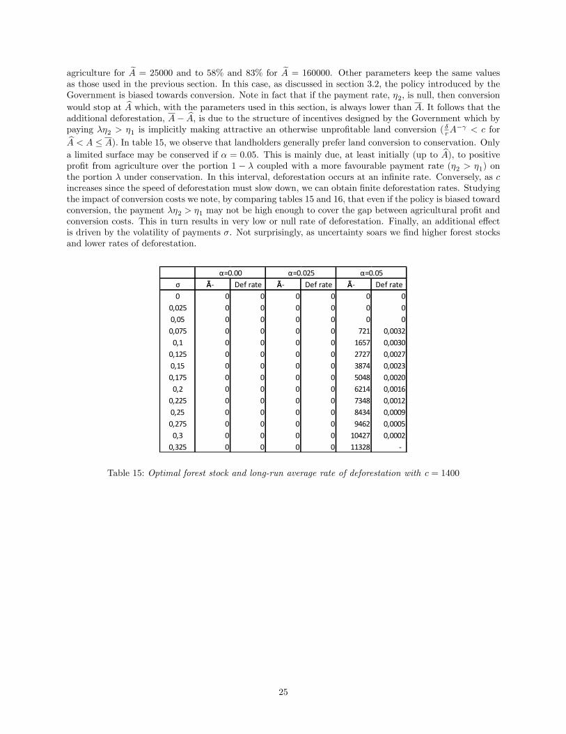
agriculture for eA = 25000 and to 58% and 83% for eA = 160000. Other parameters keep the same valuesas those used in the previous section. In this case, as discussed in section 3.2, the policy introduced by theGovernment is biased towards conversion. Note in fact that if the payment rate, �2, is null, then conversionwould stop at bA which, with the parameters used in this section, is always lower than A. It follows that theadditional deforestation, A� bA, is due to the structure of incentives designed by the Government which bypaying ��2 > �1 is implicitly making attractive an otherwise unpro�table land conversion (
�rA
� < c forbA < A � A). In table 15, we observe that landholders generally prefer land conversion to conservation. Onlya limited surface may be conserved if � = 0:05. This is mainly due, at least initially (up to bA), to positivepro�t from agriculture over the portion 1 � � coupled with a more favourable payment rate (�2 > �1) onthe portion � under conservation. In this interval, deforestation occurs at an in�nite rate. Conversely, as cincreases since the speed of deforestation must slow down, we can obtain �nite deforestation rates. Studyingthe impact of conversion costs we note, by comparing tables 15 and 16, that even if the policy is biased towardconversion, the payment ��2 > �1 may not be high enough to cover the gap between agricultural pro�t andconversion costs. This in turn results in very low or null rate of deforestation. Finally, an additional e¤ectis driven by the volatility of payments �. Not surprisingly, as uncertainty soars we �nd higher forest stocksand lower rates of deforestation.
σ ĀÃ Def rate ĀÃ Def rate ĀÃ Def rate0 0 0 0 0 0 0
0,025 0 0 0 0 0 00,05 0 0 0 0 0 00,075 0 0 0 0 721 0,0032
0,1 0 0 0 0 1657 0,00300,125 0 0 0 0 2727 0,00270,15 0 0 0 0 3874 0,00230,175 0 0 0 0 5048 0,0020
0,2 0 0 0 0 6214 0,00160,225 0 0 0 0 7348 0,00120,25 0 0 0 0 8434 0,00090,275 0 0 0 0 9462 0,0005
0,3 0 0 0 0 10427 0,00020,325 0 0 0 0 11328
α=0.00 α=0.025 α=0.05
Table 15: Optimal forest stock and long-run average rate of deforestation with c = 1400
25
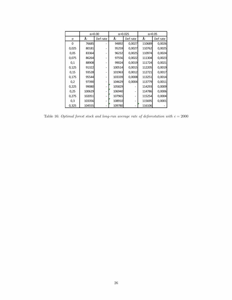
σ ĀÃ Def rate ĀÃ Def rate ĀÃ Def rate0 76685 94892 0,0027 110689 0,0026
0,025 80181 95259 0,0027 110762 0,00250,05 83364 96232 0,0025 110974 0,00240,075 86264 97556 0,0022 111304 0,0023
0,1 88908 99024 0,0019 111724 0,00210,125 91322 100514 0,0015 112205 0,00190,15 93528 101963 0,0012 112721 0,00170,175 95544 103339 0,0008 113251 0,0014
0,2 97390 104629 0,0004 113779 0,00110,225 99080 105829 114293 0,00090,25 100629 106940 114786 0,00060,275 102051 107965 115254 0,0004
0,3 103356 108910 115695 0,00010,325 104555 109780 116106
α=0.00 α=0.025 α=0.05
Table 16: Optimal forest stock and long-run average rate of deforestation with c = 2000
26
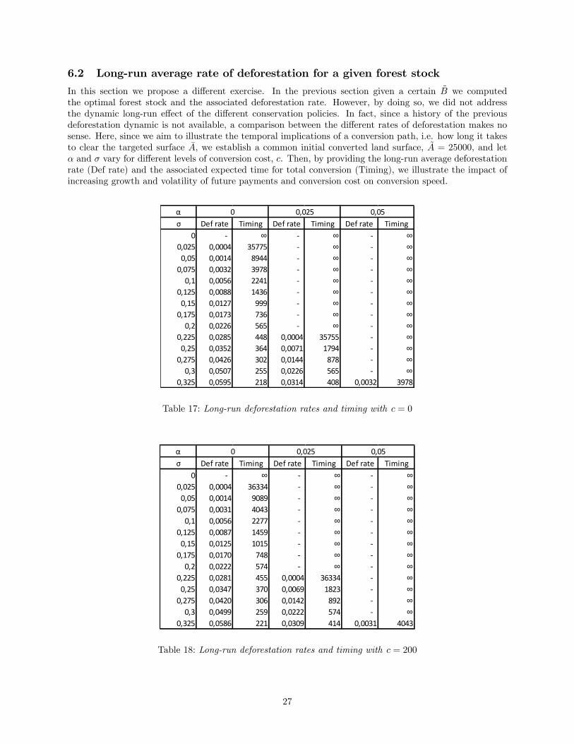
6.2 Long-run average rate of deforestation for a given forest stock
In this section we propose a di¤erent exercise. In the previous section given a certain ~B we computedthe optimal forest stock and the associated deforestation rate. However, by doing so, we did not addressthe dynamic long-run e¤ect of the di¤erent conservation policies. In fact, since a history of the previousdeforestation dynamic is not available, a comparison between the di¤erent rates of deforestation makes nosense. Here, since we aim to illustrate the temporal implications of a conversion path, i.e. how long it takesto clear the targeted surface �A, we establish a common initial converted land surface, ~A = 25000, and let� and � vary for di¤erent levels of conversion cost, c. Then, by providing the long-run average deforestationrate (Def rate) and the associated expected time for total conversion (Timing), we illustrate the impact ofincreasing growth and volatility of future payments and conversion cost on conversion speed.
ασ Def rate Timing Def rate Timing Def rate Timing
0 ∞ ∞ ∞0,025 0,0004 35775 ∞ ∞
0,05 0,0014 8944 ∞ ∞0,075 0,0032 3978 ∞ ∞
0,1 0,0056 2241 ∞ ∞0,125 0,0088 1436 ∞ ∞
0,15 0,0127 999 ∞ ∞0,175 0,0173 736 ∞ ∞
0,2 0,0226 565 ∞ ∞0,225 0,0285 448 0,0004 35755 ∞
0,25 0,0352 364 0,0071 1794 ∞0,275 0,0426 302 0,0144 878 ∞
0,3 0,0507 255 0,0226 565 ∞0,325 0,0595 218 0,0314 408 0,0032 3978
0 0,025 0,05
Table 17: Long-run deforestation rates and timing with c = 0
ασ Def rate Timing Def rate Timing Def rate Timing
0 ∞ ∞ ∞0,025 0,0004 36334 ∞ ∞
0,05 0,0014 9089 ∞ ∞0,075 0,0031 4043 ∞ ∞
0,1 0,0056 2277 ∞ ∞0,125 0,0087 1459 ∞ ∞
0,15 0,0125 1015 ∞ ∞0,175 0,0170 748 ∞ ∞
0,2 0,0222 574 ∞ ∞0,225 0,0281 455 0,0004 36334 ∞
0,25 0,0347 370 0,0069 1823 ∞0,275 0,0420 306 0,0142 892 ∞
0,3 0,0499 259 0,0222 574 ∞0,325 0,0586 221 0,0309 414 0,0031 4043
0,050 0,025
Table 18: Long-run deforestation rates and timing with c = 200
27
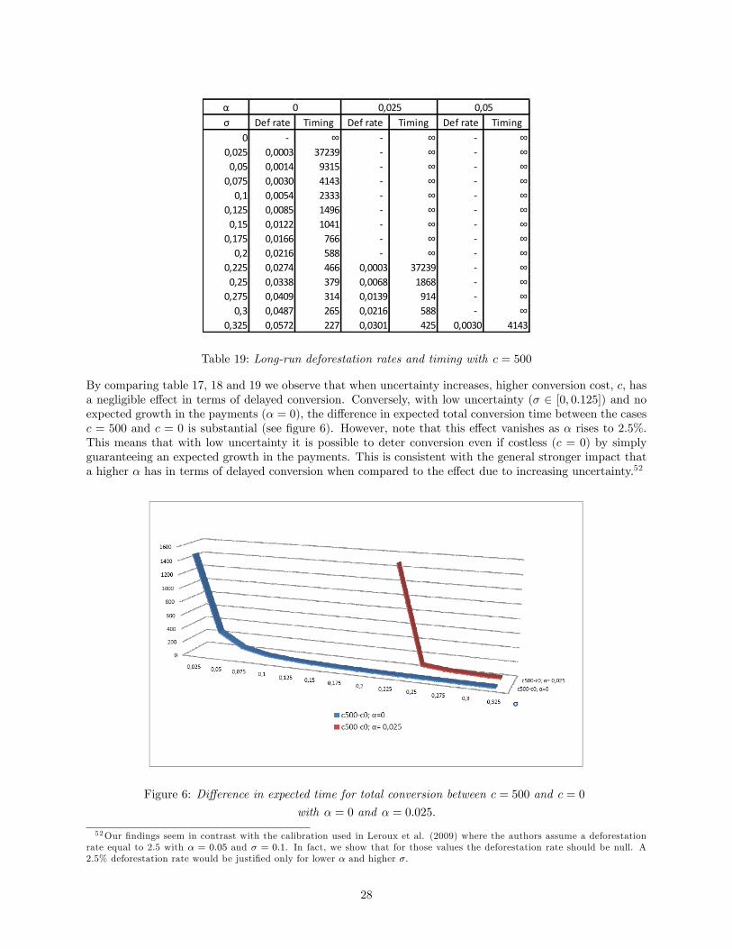
ασ Def rate Timing Def rate Timing Def rate Timing
0 ∞ ∞ ∞0,025 0,0003 37239 ∞ ∞
0,05 0,0014 9315 ∞ ∞0,075 0,0030 4143 ∞ ∞
0,1 0,0054 2333 ∞ ∞0,125 0,0085 1496 ∞ ∞
0,15 0,0122 1041 ∞ ∞0,175 0,0166 766 ∞ ∞
0,2 0,0216 588 ∞ ∞0,225 0,0274 466 0,0003 37239 ∞
0,25 0,0338 379 0,0068 1868 ∞0,275 0,0409 314 0,0139 914 ∞
0,3 0,0487 265 0,0216 588 ∞0,325 0,0572 227 0,0301 425 0,0030 4143
0 0,025 0,05
Table 19: Long-run deforestation rates and timing with c = 500
By comparing table 17, 18 and 19 we observe that when uncertainty increases, higher conversion cost, c, hasa negligible e¤ect in terms of delayed conversion. Conversely, with low uncertainty (� 2 [0; 0:125]) and noexpected growth in the payments (� = 0), the di¤erence in expected total conversion time between the casesc = 500 and c = 0 is substantial (see �gure 6). However, note that this e¤ect vanishes as � rises to 2:5%.This means that with low uncertainty it is possible to deter conversion even if costless (c = 0) by simplyguaranteeing an expected growth in the payments. This is consistent with the general stronger impact thata higher � has in terms of delayed conversion when compared to the e¤ect due to increasing uncertainty.52
Figure 6: Di¤erence in expected time for total conversion between c = 500 and c = 0
with � = 0 and � = 0:025.
52Our �ndings seem in contrast with the calibration used in Leroux et al. (2009) where the authors assume a deforestationrate equal to 2.5 with � = 0:05 and � = 0:1. In fact, we show that for those values the deforestation rate should be null. A2.5% deforestation rate would be justi�ed only for lower � and higher �:
28
7 Conclusions
In this paper we contribute to the vast literature on optimal land allocation under uncertainty and irreversiblehabitat conversion. We extend previous work in three respects. First, departing from the standard centralplanner perspective we investigate the role that competing farming may have on conversion dynamics. Pro�tsfrom conversion decreasing in the number of developers may discourage conversion in particular if societyis willing to reward habitat conservation as land use. Second, in this decentralized framework, we look atthe conservation e¤ort that Government land policy, through a combination of voluntary and commandapproaches, may stimulate.In this regard, an interesting result is represented by the considerable amount of conservation that the
Government can induce by partially compensating agents for the ES provided.In addition, we show that the existence of a ceiling for the stock of developable land may produce perverse
e¤ects on conversion dynamics by activating a run which instantaneously exhausts the stock. Third, webelieve that time matters when dynamic land allocation is analysed. Hence, we suggest the use of theoptimal long-run average expected rate of conversion to assess the temporal performance of conservationpolicy and we show its utility by running several numerical simulations based on realistic policy scenarios.
29
A Appendix
A.1 Equilibrium under �1 > ��2The value function of a farmer is given by:
V (A;B; �A) = Z2(A)B�2 +
(1� �)�r
A� + (��2 � �1)B
r � � (A.1.1)
Since each agent rationally forecasts the future dynamics of the market for agricultural goods at B�(A)she/he must be indi¤erent between conserving and converting. That is:
Z2(A)B�(A)
�2+(1� �)�
rA� + (��2 � �1)
B�(A)
r � � = (1� �)c (A.1.2)
In addition, the following conditions must hold (see e.g. proposition 1 in Bartolini (1993) and Grenadier(2002, p. 699)):
VA(A;B�(A); �A) = Z 02(A)B
�(A)�2 � (1� �)� A�( +1)
r= 0 (A.1.3)
and
@V (A;B�(A); �A)
@A= VA(A;B
�(A); �A) + VB(A;B�(A); �A)
dB�(A)
dA(A.1.4)
=
��2Z2 (A)B
�(A)�2�1+
��2 � �1r � �
�dB�(A)
dA= 0
Finally, considering the limit on conversion, �A; imposed by the Government it follows that:
Z2( �A) = 0 (A.1.5)
Condition (A.1.4) illustrates two scenarios. In the �rst one, each landholder exercises the option to convertat the level of B�(A) where the value, V (A;B�(A); �A) is tangent to the conversion cost, (1� �) c.53 Thatis, VB(A;B�(A); �A) = �2Z2(A)B
�(A)�2�1
+ ��2��1r�� = 0. It is easy to verify that, as conjectured, Z2(A) < 0.
In the case V (A,B�(A); �A) is smooth at the conversion threshold and B�(A) is a continuous function ofA. In the second scenario, the optimal threshold B�(A) does not vary with A, i.e. VB(A,B�(A); �A) 6= 0
and dB�(A)dA = 0. This implies that the landholder may bene�t from marginally anticipating or delaying the
conversion decision. In particular, if VB(A,B�(A); �A) < 0 then the value of conversion is expected to increaseas B drops. Conversely, if VB(A,B�(A); �A) > 0 then losses must be expected as B drops. However, in bothcases (A.1.4) holds by imposing dB�(A)
dA = 0.By (A.1.4) we can split [A0; �A] into two intervals where one of the following two conditions must hold:
�2Z2 (A)B�(A)�2�1 +
��2 � �1r � � = 0 (A.1.6)
dB�(A)
dA= 0 (A.1.7)
Since Z2��A�= 0 and ��2��1
r�� < 0, then (A.1.6) cannot hold at A = �A. Therefore, (A.1.7) must hold atA = �A and by (A.1.2) it follows that:
B�( �A) = (r � �)"(A�A) � 1
#c for A+ � A � �A (A.1.8)
where A = ( �rc )1= represents the last parcel conversion which makes economic sense. In fact, note that since
(��2 � �1) Br�� < 0 then
�rA
� � c for A � A.53This condition holds at any re�ecting barrier without any optimization being involved (Dixit, 1993).
30

Now let�s de�ne A+ as the largest A � �A that satis�es (A.1.6). This implies that for all the landholdersin the range A+ � A � �A, we have dB�(A)
dA = 0 and conversion takes place at B�( �A). Over the range A < A+
(A.1.3) holds by de�nition. Hence, plugging (A.1.6) into (A.1.4) we obtain:
B�(A) =�2
�2 � 1(r � �)
"(A
A) � 1
#c for A < A+ (A.1.9)
Finally, by the continuity of B�(A) follows that B�(A+) = B�( �A).Substituting:
�2�2 � 1
(r � �)"(A
A+) � 1
#c = (r � �)
"(A�A) � 1
#c (A.1.10)
where
A+ = [(�2 � 1) �A� + A�
�2]�
1
The conversion policy is summarized by (A.1.8) and (A.1.9). The conversion policy should be smooth untilthe surface A+ < �A has been converted. At A+ landholders rush and a run takes place to convert the residualland before the limit imposed by the Government is met. By (A.1.9), B�(A) is decreasing with respect to A.This makes sense since further land conversion reduces the pro�t from agriculture and a landholder wouldconvert land only if she/he expects a future reduction in B.We must investigate two di¤erent scenarios, i.e. A � �A and A > �A. From (A.1.10) it follows that:
�2�2 � 1
"(A
A+) � 1
#= (
A�A) � 1 (A.1.10 bis)
Studying (A.1.10 bis) we can state that since �2�2�1
> 0:
- if A � �A then it must be �A � A+. This implies that there is no run taking place. Land will be convertedsmoothly according to (A.1.8) up to A since �
rA� � c for A � A;
- if A > �A then it must be A+ < �A. In this case, land is converted smoothly up to A+ where landholdersstart a run to convert land up to �A.
A.2 Value of the option to convert
In this appendix we show that, by competition, the value of the opportunity to develop the plot by the singlefarmer is null at the conversion threshold. The value of the option to convert, F (A,B; �A), is the solution ofthe following di¤erential equation (Dixit and Pindyck, 1994, ch. 8):
1
2�2B2FBB(A;B; �A) + �BFB(A;B; �A)� rF (A;B; �A) = 0 for B > BC(A) (A.2.1)
where BC(A) is the optimal threshold for conversion. Note that this is an ordinary di¤erential equation, thegeneral solution of which can be written as:
F (A;B; �A) = C1(A)B�1 + C2(A)B
�2 (A.2.2)
where 1 < �1 < r=�, �2 < 0 are the positive and the negative root of the characteristic equation (�) =12�
2�(� � 1) + �� � r = 0, and C1, C2 are two constants to be determined.Suppose for instance that �1 > ��2.
54 This implies that as B increases, the value of the option toconvert should vanish as (limB!1 F (A;B; �A) = 0) then we set C1 = 0. Now, let�s determine the optimal
54 It is easy to show that the results in this section would hold also for the case �1 < �2�:
31
conversion threshold B and the constant C1(A). We attach to the di¤erential equation above the followingvalue matching and the smooth pasting conditions:
F (A;BC(A); �A) = V (A;BC(A); �A)� (1� �) c (A.2.3)
C2(A)BC(A)�2 = Z2(A)B
C(A)�2 +(1� �) �A�
r+(��2 � �1)BC(A)
r � � � (1� �) c
FB(A;BC(A); �A) = VB(A;B
C(A); �A) (A.2.4)
�2C2(A)BC(A)�2�1 = �2Z2(A)B
C(A)�2�1 +��2 � �1r � �
It follows that:
BC(A)=B�(A) =�2
�2 � 1(r � �)[�
rA� � c]
From (A.1.4) we obtain VB(A;B�(A); �A) = �2Z2(A)B�(A)
�2�1+ ��2��1
r�� = 0 which in turn implies Z2(A) =
���2��1r��
B�(A)1��2
�2.
Rearranging (A.2.4) and substituting we have:
C(A) = Z2(A) +��2 � �1r � �
BC(A)1��2
�2
=��2 � �1(r � �)�2
(BC(A)1��2 �B�(A)1��2) = 0
As expected the value of the option to convert is null at BC(A) = B�(A).
A.3 Equilibrium under �1 < ��2The value function of a farmer is given by:
V (A;B; �A) = Z1(A)B�1 +
(1� �)�r
A� + (��2 � �1)B
r � � (A.3.1)
As in section A.1 the following conditions must hold at B��(A)
Z1(A)B��(A)
�1+(1� �)�
rA� + (��2 � �1)
B��(A)
r � � = (1� �)c (A.3.2)
VA(A;B��(A); �A)=Z 01(A)B
��(A)�1 � (1� �)�A�( +1)
r= 0 (A.3.3)
@V (A;B��(A); �A)
@A= VA(A;B
��(A); �A) + VB(A;B��(A); �A)
dB��(A)
dA(A.3.4)
=
��1Z1 (A)B
��(A)�1�1 +��2 � �1r � �
�dB��(A)
dA= 0
In addition, since land can be converted only up to �A then it follows that:
Z1( �A) = 0 (A.3.5)
Condition (A.3.4) illustrates two scenarios. In the �rst one, each landholder exercises the option to convertat the level of B��(A) where the value, V (A;B��(A); �A) is tangent to the conversion cost, (1� �) c. That is,VB(A;B
��(A); �A) = �1Z1(A)B�(A)
�1�1+ ��2��1
r�� = 0. Since ��2��1r�� > 0 it can be can easily veri�ed that,
as conjectured, Z1(A) < 0. In the case V (A;B��(A); �A) is smooth at the conversion threshold and B��(A)is a continuous function of A. In the second scenario, the optimal threshold B��(A) does not change with
32
A, i.e. VB(A;B��(A); �A) 6= 0 and dB��(A)dA = 0. As discussed in section A.1, this implies that at the margin
the landholder may bene�t from anticipating or delaying the conversion decision.By (A.3.4) the set [A0; �A] can be split into two subsets where one of the following two conditions must
hold:
�1Z1 (A)B��(A)�1�1 +
��2 � �1r � � = 0 (A.3.6)
dB��(A)
dA= 0 (A.3.7)
Note that as Z1��A�= 0 and ��2��1
r�� > 0, then (A.3.6) cannot hold at A = �A. Therefore, (A.3.7) must holdat A = �A. From (A.3.2) it follows that:
B��( �A) = (r � �) "1� ( A�A
)
#c for A++ < A � �A (A.3.8)
We now de�ne A++ as the largest A � �A for which (A.3.6) holds. This means that for all the landholdersin the range A++ � A � �A, we must have dB��(A)
dA = 0 and conversion occurs at B��( �A). Over the rangeA < A++ (A.3.3) holds by de�nition. Then, substituting (A.3.6) into (A.3.4) we get:
B��(A) =�1
�1 � 1(r � �)
"1� ( A
A)
#c for A0 < A � A++ (A.3.9)
However, note that B��(A) < 0 for A < A. Since by (2) B cannot be negative then it must be:
B��(A) =
(0; for A0 < A � A�1�1�1
(r � �) h1� ( AA )
ic; for A < A � A++ (A.3.9 bis)
By continuity of B��(A) it follows that B��(A++) = B��( �A). Substituting:
�1�1 � 1
(r � �) "1� ( A
A++)
#c = (r � �)
"1� ( A�A
)
#c (A.3.10)
where
A+ = [(�1 � 1) �A� + A�
�1]�
1
From (A.3.10) it follows that:�1
�1 � 1[1� ( A
A++) ] = 1� ( A�A
) (A.3.10 bis)
As in section (A.1), two di¤erent scenarios may arise. In fact, studying (A.3.10 bis) we observe that since�1�1�1
> 0:
- if A � �A then it must be A � A++ � �A. Land will be converted according to (A.3.9 bis) up to A++. AtA++ landholders will rush to convert land up to the limit, �A, established by the Government (A.3.8);
- if A > �A then it must be A > A++ > �A. This implies that the conversion process follows (A.3.9 bis) andland is instantaneously developed up to �A.
A.4 Long-run distributions
Let h be a linear Brownian motion with parameters � and � that evolves according to dh = �dt + �dw.Following Harrison (1985, pp. 90-91; see also Dixit 1993, pp. 58-68) the long-run density function for h
33

�uctuating between a lower re�ecting barrier, a 2 (�1;1), and an upper re�ecting barrier, b 2 (�1;1),is represented by the following truncated exponential distribution:
f (h) =
8<: 2��2
e2�
�2h
e2�
�2b�e
2�
�2a
� 6= 01b�a � = 0:
(A.4.1)
We are interested to the limit case where a! �1: In this case, from (A.4.1) a limiting argument gives:
f (h) =
�2��2 e
� 2�
�2(b�h) � > 0
0 � � 0:for �1 < h < b (A.4.2)
Hence, the long-run average of h can be evaluated as E [h] =R�hf (h) dh, where � depends on the distrib-
ution assumed. In the steady-state this yields:
E [h] =
Z b
�1hf (h) dh =
Z b
�1h2�
�2e�
2�
�2(b�h)dh =
2�
�2e�
2�
�2b
Z b
�1he
2�
�2hdh = b� 2�
�2(A.4.3)
A.5 Long-run average growth rate of deforestation
Taking the logarithm of (16) we get:
ln � = ln
��2
�2 � 1(1� �) PA (A)
r� �1 � ��2
r � � B
�(A.5.1)
= ln
��1 � ��2r � �
�+ ln [J �B]
where J= �2�2�1
(r � �)PA(A)r and J > B. Rewriting ln [J �B] as ln
�eln J � elnB
�and expanding it by
Taylor�s theorem around the point (glnJ;glnB) yields:ln [J �B] ' v0 + v1 lnJ + v2 lnB
where
v0 = lnhegln J � eglnBi� " glnJ
1� eglnB�gln J +glnB
1� e�(glnB�gln J)#
v1 =1
1� eglnB�gln J ; v2 =1
1� e�(glnB�gln J) ;v2v1=1� v1v1
< 0
By substituting the approximation into (A.5.1) it follows that:
ln � ' ln �1 � ��2r � � + v0 + v1 lnJ + v2 lnB (A.5.2)
Now, by Ito�s lemma and the considerations discussed in the paper on the competitive equilibrium, ln �evolves according to d ln � = v2d lnB = v2[(�� 1
2�2)dt+ �dw] with ln � as upper re�ecting barrier. Setting
h = ln �, the random variable ln � follows a linear Brownian motion with parameter � = v2(� � 12�
2) > 0and has a long-run distribution with (A.4.2) as density function.Solving (A.5.2) with respect to lnA we obtain the long-run optimal stock of deforested land, i.e.:
lnA 'lnh�1���2r��
i+ v0 + v1 ln
h�2�2�1
(r � �) �r
i+ v2 lnB � h
v1(A.5.3)
From (A.5.3) by some manipulations we can show that
34
1 = exp(v0v1)(
�1���2r��
�)1v1
��2
�2 � 1(r � �)�
r
�A� B
v2v1
= exp(v0v1)
��2
�2 � 1(r � �)
�� v2v1 �
rc�
1v1A� B
v2v1
= exp(v0v1)(
J�rA
� )� v2v1�
rc�
1v1A� B
v2v1
= exp(v0v1)J�
v2v1 (
�
rcA� )
1v1B
v2v1
= exp(v0)J�v2(
A
A) Bv2
=eJ � eBeJv1 eBv2 J�v2( AA ) Bv2
= (~A
A)(BeB )� 1
h1�( ~A
A) i
andA~A= (
BeB )� 1
h1�( ~A
A) i
Note that since ~A < A then � 1
h1� ( ~A
A) i< 0.
Taking the expected value on both sides of (A.5.3) leads to:
E [lnA] 'lnh�1���2r��
i+ v0 + v1 ln
h�2�2�1
(r � �) �r
i+ v2
�B0 + (�� 1
2�2)t�� E [h]
v1
Since by (A.4.3) E(h) is independent on t, di¤erentiating with respect to t, we obtain the expected long-runrate of deforestation:
1
dtE [d lnA] ' v2
v1
�� 12�
2
= ��� 1
2�2
eglnB�gln J for � <
1
2�2
By the monotonicity property of the logarithm, eB must exists such that ln eB = glnB. Furthermore, byplugging eB into (10), we can always �nd a surface ~A and eJ = �2
�2�1(r � �)PA( ~A)
r such that a linearization
along (glnB;glnJ) is equivalent to a linearization along (ln eB; ln eJ), where glnJ = ln eJ . This implies that bysetting ( eB; ~A), the long-run average rate of deforestation can be written as:
1
dtE [d lnA] = �
�� 12�
2
eBeJ = ��� 1
2�2
1
1 + �2�2�1
(r � �) ceB= �
�� 12�
2
PA( ~A)r � cPA( ~A)r
= ��� 1
2�2
(1� c
�r~A�
)
wherePA( ~A)r =
eB�2
�2�1(r��)
+ c and ~A < A.
Similarly, from the logarithm of (18) we derive:
ln & = ln
��1
�1 � 1(1� �) PA
r+��2 � �1r � � B
�(A.5.4)
= ln
���2 � �1r � �
�+ ln [K +B]
35
where K= �1�1�1
(r � �) PA(A)r and K > �B. Rewriting ln [K +B] as ln�elnK + elnB
�and expanding by
Taylor�s theorem around the point (glnK;glnB) leads to:ln [K +B] ' ln
heglnK + eglnBi+ lnK � glnK
1 + eglnB�glnK +lnB � glnB
1 + e�(glnB�glnK)= w0 + w1 lnK + w2 lnB
where
w0 = lnheglnK + eglnBi� " glnK
1 + eglnB�glnK +glnB
1 + e�(glnB�glnK)#
w1 =1
1 + eglnB�glnK ; w2 = 1
1 + e�(glnB�glnK) ; w2w1 =1� w1w1
> 0
By plugging the approximated value for ln [K +B] into (A.5.4) we obtain:
ln & ' ln���2 � �1r � �
�+ w0 + w1 lnK + w2 lnB (A.5.5)
Also in this case, ln & evolves according to the motion d ln & = w2d lnB = w2[(� � 12�
2)dt + �dw] andln & is a re�ecting barrier. By setting h = ln &, ln & evolves as a linear Brownian motion with parameter� = w2(�� 1
2�2) > 0 and (A.4.2) as density function. Then, solving (A.5.5) with respect to lnA yields the
long-run optimal stock of cleared land:
lnA 'lnh��2��1(r��)
i+ w0 + w1 ln
h�1�1�1
(r � �) �ri+ w2 lnB � h
w1(A.5.6)
As above, from (A.5.6) it follows that
1 = exp(w0w1)(
��2��1r��&
)1w1
��1
�1 � 1(r � �) �
r
�A� B
w2w1
= exp(w0w1)
��1
�1 � 1(r � �)
��w2w1 �
rc�
1w1A� B
w2w1
= exp(w0w1)(
K�rA
� )�w2w1�
rc�
1w1A� B
w2w1
= exp(w0w1)K�w2
w1 (�
rcA� )
1w1B
w2w1
= exp(w0)K�w2(
A
A) Bw2
=eK + eBeKw1 eBw2K�w2(
A
A) Bw2
= (~A
A)(BeB )� 1
h1�( ~A
A) i
andA~A= (
BeB )� 1
h1�( ~A
A) i
Note that since in this case ~A > A then � 1
h1� ( ~A
A) i> 0.
From (A.5.6) the expected value of lnA is given by:
E [lnA] 'lnh��2��1r��
i+ w0 + w1 ln
h�1�1�1
(r � �) �r
i+ w2
�B0 + (�� 1
2�2)t�� E [h]
w1
36
By the usual steps:
1
dtE [d lnA] ' w2
w1
�� 12�
2
=�� 1
2�2
eglnB�glnK for � >
1
2�2
As shown above, having �xed a pair ( eB; ~A) we can conveniently linearize along (ln eB; ln eJ) where ln eB = glnBand glnK = ln eK with eK= �1
�1�1(r � �) 1��
�2���1PA( ~A)r . This leads to the following expression for the long-run
average rate of deforestation:
1
dtE [d lnA] =
�� 12�
2
eBeK =�� 1
2�2
1�1�1�1
(r � �) ceB � 1=
�� 12�
2
c� PA( ~A)r
PA( ~A)r
=�� 1
2�2
(
c�r~A�
� 1)
wherePA( ~A)r = c� eB
�1�1�1
(r��)and ~A > A.
A.6 The impact of uncertainty on the distribuition of � (and &)
Rearranging (A.5.2) yieldsln � ' U� + v2 lnB (A.6.1)
where U� = ln�1���2r�� + v0 + v1 lnJ:
By some manipulations:
eln � = eU�+v2 lnB
� = eU�Bv2 (A.6.2)
Using Ito�s lemma
d� = eU��v2B
v2�1dB +1
2v2(v2 � 1)Bv2�2(dB)2
�= eU�Bv2v2
���+
1
2(v2 � 1)�2
�dt+ �dw
�= �v2
���+
1
2(v2 � 1)�2
�dt+ �dw
�Calculating �rst, second moment and variance for � we obtain:
E(�) = �(0)ev2[�+12 (v2�1)�
2]t
E(�2) = �2(0)e2v2[�+(v2�12 )�
2]t
V ar(�) = �2(0)e2v2[�+12 (v2�1)�
2]t(ev22�
2t � 1)
Note that since � + 12 (v2 � 1)�
2 < 0 and v2 < 0 then E(�) is increasing in t. Finally, by deriving V ar(�)with respect to � it is easy to check that
@V ar(�)
@�= 2v2�te
2v2[�+ 12 (v2�1)�
2]t�2(0)h(v2�1)(e
v22�2t�1) + v2e
v22�2ti> 0
That is, as � soars V ar(�) increases and so does the probability of hitting � which in turn implies an increasein the long run average deforestation rate.
37

Similarly, starting from (A.5.5)ln & ' U& + w2 lnB (A.6.3)
where U& = lnh��2��1r��
i+ w0 + w1 lnK, one may easily check that
V ar(&) = &2(0)e2w2[�+12 (w2�1)�
2]t(ew22�
2t � 1)
and
@V ar(&)
@�= 2w2�te
2w2[�+ 12 (w2�1)�
2]t&2(0)h(w2�1)(e
w22�2t�1) + w2e
w22�2ti< 0
38
References
[1] Adler. J.H., 2008. Money or nothing: the adverse environmental consequences of uncompensated land-use controls. Boston College Law Review, 49, 2, 301-366.
[2] Arrow, K.J., Fisher, A.C., 1974. Environmental preservation, uncertainty, and irreversibility. QuarterlyJournal of Economics, 88, 312-319.
[3] Bartolini L., 1993. Competitive runs, the case of a ceiling on aggregate investment. European EconomicReview, 37, 921-948.
[4] Baldursson, F. M., 1998. Irreversible investment under uncertainty in oligopoly. Journal of EconomicDynamics and Control, 22, 627-644.
[5] Bentolila, S., Bertola, G., 1990. Firing costs and labour demand: how bad is eurosclerosis? Review ofEconomic Studies, 57, 3, 381-402.
[6] Bulte, E., van Soest, D.P., van Kooten, G.C., and R.A., Schipper, 2002. Forest conservation in CostaRica when nonuse bene�ts are uncertain but rising. American Journal of Agricultural Economics, 84,1, 150-160.
[7] Bulte, E., Rondeau, D., 2005. Why compensating wildlife damages may be bad for conservation. Journalof Wildlife Management, 69, 1,14-19.
[8] Bulte, E., Rondeau, D., 2007. Wildlife damage and agriculture: a dynamic analysis of compensationschemes. American Journal of Agricultural Economics, 89, 2, 490-507.
[9] Butler, R.A., Koh, L.P., and J., Ghazoul, 2009. REDD in the red: palm oil could undermine carbonpayment schemes. Conservation Letters, 2, 67�73.
[10] Caballero, R., Pindyck, R.S., 1992. Uncertainty, investment and industry Evolution. NBER workingPaper no. 4160.
[11] Clarke, H.R., Reed, W.J., 1989. The tree-cutting problem in a stochastic environment. Journal ofEconomic Dynamics and Control, 13, 569-595.
[12] Conrad, J.M., 1980. Quasi-option value and the expected value of information. Quarterly Journal ofEconomics, 95, 813-820.
[13] Conrad, J.M., 1997. On the option value of old-growth forest. Ecological Economics, 22, 97-102.
[14] Conrad, J.M., 2000. Wilderness: options to preserve, extract, or develop. Resource and Energy Eco-nomics, 22, 3, 205-219.
[15] Cox, J.C., Ross, S.A., 1976. The valuation of options for alternative stochastic process. Econometrica,53, 385�408.
[16] Dixit, A., 1989. Entry and exit decisions under uncertainty. Journal of Political Economy, 97, 620�638.
[17] Dixit, A., 1993. The Art of Smooth Pasting. Switzerland: Harwood Academic Publishers.
[18] Dixit, A., Pindyck, R.S., 1994. Investment under Uncertainty. Princeton (NJ), Princeton UniversityPress.
[19] Dosi, C., Moretto, M. 1997. Pollution accumulation and �rm incentives to promote irreversible techno-logical change under uncertain private bene�ts. Environmental and Resource Economics, 10, 285-300.
[20] Engel, S., Pagiola, S., and S. Wunder, 2008. Designing payments for environmental services in theoryand practice: an overview of the issues. Ecological Economics, 65, 663�674.
[21] Fargione, J., Hill J., Tilman D., Polasky S., and P., Hawthorne, 2008. Land clearing and the biofuelcarbon debt. Science, 319, 1235�1238.
39
[22] Ferraro, P.J., 2001. Global habitat protection: limitations of development interventions and a role forconservation performance payments. Conservation Biology, 15, 990-1000.
[23] Ferraro, P.J., Kiss, A., 2002. Direct payments to conserve biodiversity. Science, 298, 1718-1719.
[24] Ferraro, P.J., Simpson, R.D., 2002. The cost-e¤ectiveness of conservation payments. Land Economics,78, 3, 339-353.
[25] Ferraro, P.J., Simpson, R.D., 2005. Protecting forests and biodiversity: are investments in eco-friendlyproduction activities the best way to protect endangered ecosystems and enhance rural livelihoods?Forests, Trees and Livelihoods, 15, 167-181.
[26] Ferraro, P.J., Pattanayak, S., 2006. Money for nothing? A call for empirical evaluation of biodiversityconservation investments. PLoS Biol 4(4): e105. doi:10.1371/journal.pbio.0040105.
[27] Ferraro, P.J., 2008. Asymmetric information and contract design for payments for environmental ser-vices. Ecological Economics, 65, 4, 810-821.
[28] Fitzherbert, E.B., Struebig, M.J., Morel, A., Danielsen, F., Brühl, C.A., Donald, P.F., and B. Phalan,2008. How will oil palm expansion a¤ect biodiversity? Trends in Ecology & Evolution, 23, 538�545.
[29] Folke, C., Holling, C.S., and C. Perrings, 1996. Biological Diversity, Ecosystems, and the Human Scale.Ecological Applications, 6, 4, 1018-1024
[30] FONAFIFO, 2007. Manual de Procedimientos para el pago de Servicios Ambientales. Gaceta, 51,13/03/2007. http://www.fona�fo.com/text_�les/servicios_ambientales/Manuales/MPPSA_2007.pdf
[31] Grenadier, S.R., 2002. Option exercise games: an application to the equilibrium investment strategiesof �rms. Review of Financial Studies, 15, 691-721.
[32] Hansen, A.J., Rotella, J.J., 2002. Biophysical factors, land use, and species viability in and aroundnature reserves. Conservation Biology, 16, 4, 1112�1122.
[33] Hansen, A.J., DeFries, R., 2007. Ecological mechanisms linking protected areas to surrounding lands.Ecological Applications, 17, 4, 974�988.
[34] Harrison, J.M., 1985, Brownian Motion and Stochastic Flow Systems. New York: John Wiley & Sons.
[35] Hartman R., Hendrickson M., 2002. Optimal Partially Reversible Investment. Journal of EconomicDynamics and Control, 26, 483�508.
[36] Henry, C., 1974. Investment decisions under uncertainty: the "Irreversibility E¤ect". American Eco-nomic Review, 64, 6, 1006-1012.
[37] Hopenhayn, H., 1992. Entry, exit and �rm dynamics in long run equilibrium. Econometrica, 60, 1127�1150.
[38] IPCC, 2007. Climate Change 2007: The Fourth Assessment Report of the Intergovernmental Panel onClimate Change. Cambridge Univ. Press, Cambridge.
[39] Isik, M., Yang, W., 2004. An analysis of the e¤ects of uncertainty and irreversibility on farmer partic-ipation in the conservation reserve program. Journal of Agricultural and Resource Economics, 29, 2,242�259.
[40] Jovanovic, B., 1982. Selection and the evolution of industry. Econometrica, 50, 649�670.
[41] Kassar, I., Lasserre, P., 2004. Species preservation and biodiversity value: a real options approach.Journal of Environmental Economics and Management, 48, 2, 857-879.
[42] Koh, L.P., Ghazoul, J., 2008. Biofuels, biodiversity, and people: understanding the con�icts and �ndingopportunities. Biological Conservation, 141, 2450�2460.
40
[43] Lambson, V.E., 1992. Competitive pro�ts in the long run. Review of Economic Studies, 59, 125�142.
[44] Langpap, C., Wu, J., 2004. Voluntary conservation of endangered species: when does no regulatoryassurance mean no conservation? Journal of Environmental Economics and Management, 47, 435�457.
[45] Leroux, A.D., Martin, V.L. and T. Goesch, 2009. Optimal conservation, extinction debt,and the aug-mented quasi-option value. Journal of Environmental Economics and Management, 58, 43�57.
[46] Lucas, R.E. Jr, Prescott, E.C., 1971. Investment under uncertainty. Econometrica, 39, 659-681.
[47] Mæstad, O., 2001. Timber trade restrictions and tropical deforestation: a forest mining approach.Resource and Energy Economics, 23, 2, 111-132
[48] Moretto, M., 2008. Competition and irreversible investment under uncertainty. Information Economicsand Policy, 20, 1, 75-88.
[49] Pagiola, S., 2008. Payments for environmental services in Costa Rica. Ecological Economics, 65, 4,712�724.
[50] Pearce, D., F. Putz, and J. K. Vanclay, 1999. A sustainable forest future. Working Paper GEC 99-15,CSERGE, London.
[51] Phelps, J., Guerrero, M.C., Dalabajan, D.A., Young, B. and E.L., Webb, 2010. What makes a �REDD�country? Global Environmental Change, 20, 2, 322-332.
[52] Productivity Commission, 2004. Impacts of native vegetation and biodiversity regulations. ProductivityCommission Working Paper No. 29. Available at SSRN: http://ssrn.com/abstract=600970
[53] Reed, W.J., 1993. The decision to conserve or harvest old-growth forest. Ecological Economics, 8, 45-69.
[54] Santilli, M. P., Moutinho, P., Schwartzman, S., Nepstad, D., Curran, L. and C., Nobre, 2005. Tropicaldeforestation and the Kyoto Protocol. Climate Change, 71, 267�276.
[55] Segerson, K., Miceli, T.J., 1998. Voluntary environmental agreements: good or bad news for environ-mental protection. Journal of Environmental Economics and Management, 36, 109�130.
[56] Sierra, R., Russman, E., 2006. On the e¢ ciency of environmental service payments: a forest conservationassessment in the Osa Peninsula, Costa Rica. Ecological Economics, 59, 131�141.
[57] Smith, R.B.W., Shogren, J.F., 2002. Voluntary incentive design for endangered species protection.Journal of Environmental Economics and Management, 43, 169�187.
[58] Stavins, R.N., Ja¤e, A.B., 1990. Unintended impacts of public investments on private decisions: thedepletion of forested wetlands. American Economic Review, 80, 3, 337-352.
[59] Tisdell, C.A., 1995, Issues in biodiversity conservation including the role of local communities. Environ-mental Conservation, 22, 216-222.
[60] van Vliet, O.P.R., Faaij, A.P.C., and C., Dieperink, 2003. Forestry Projects under the Clean Develop-ment Mechanism? Climate Change, 61, 123-156.
[61] Wells, M., Brandon, K.E., and L., Hannsh, 1992, People and parks: linking procteded area managementwith local communities. The World Bank, WWF, and USAID, Washington , D.C.
[62] Wunder, S., Engel, S., and S., Pagiola, 2008. Taking stock: a comparative analysis of payments forenvironmental services programs in developed and developing countries. Ecological Economics, 65, 834-853.
[63] Wunder, S. 2005. Payments for environmental services: some nuts and bolts. CIFOR Occasional paper42. Center for International Forestry Research, Bogor, Indonesia.
41
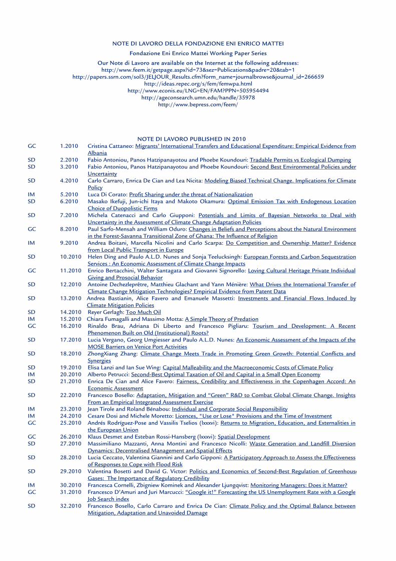
NOTE DI LAVORO DELLA FONDAZIONE ENI ENRICO MATTEI
Fondazione Eni Enrico Mattei Working Paper Series
Our Note di Lavoro are available on the Internet at the following addresses: http://www.feem.it/getpage.aspx?id=73&sez=Publications&padre=20&tab=1
http://papers.ssrn.com/sol3/JELJOUR_Results.cfm?form_name=journalbrowse&journal_id=266659 http://ideas.repec.org/s/fem/femwpa.html
http://www.econis.eu/LNG=EN/FAM?PPN=505954494 http://ageconsearch.umn.edu/handle/35978
http://www.bepress.com/feem/
NOTE DI LAVORO PUBLISHED IN 2010 GC 1.2010 Cristina Cattaneo: Migrants’ International Transfers and Educational Expenditure: Empirical Evidence from
Albania SD 2.2010 Fabio Antoniou, Panos Hatzipanayotou and Phoebe Koundouri: Tradable Permits vs Ecological Dumping SD 3.2010 Fabio Antoniou, Panos Hatzipanayotou and Phoebe Koundouri: Second Best Environmental Policies under
Uncertainty SD 4.2010 Carlo Carraro, Enrica De Cian and Lea Nicita: Modeling Biased Technical Change. Implications for Climate
Policy IM 5.2010 Luca Di Corato: Profit Sharing under the threat of Nationalization SD 6.2010 Masako Ikefuji, Jun-ichi Itaya and Makoto Okamura: Optimal Emission Tax with Endogenous Location
Choice of Duopolistic Firms SD 7.2010 Michela Catenacci and Carlo Giupponi: Potentials and Limits of Bayesian Networks to Deal with
Uncertainty in the Assessment of Climate Change Adaptation Policies GC 8.2010 Paul Sarfo-Mensah and William Oduro: Changes in Beliefs and Perceptions about the Natural Environment
in the Forest-Savanna Transitional Zone of Ghana: The Influence of Religion IM 9.2010 Andrea Boitani, Marcella Nicolini and Carlo Scarpa: Do Competition and Ownership Matter? Evidence
from Local Public Transport in Europe SD 10.2010 Helen Ding and Paulo A.L.D. Nunes and Sonja Teelucksingh: European Forests and Carbon Sequestration
Services : An Economic Assessment of Climate Change Impacts GC 11.2010 Enrico Bertacchini, Walter Santagata and Giovanni Signorello: Loving Cultural Heritage Private Individual
Giving and Prosocial Behavior SD 12.2010 Antoine Dechezleprêtre, Matthieu Glachant and Yann Ménière: What Drives the International Transfer of
Climate Change Mitigation Technologies? Empirical Evidence from Patent Data SD 13.2010 Andrea Bastianin, Alice Favero and Emanuele Massetti: Investments and Financial Flows Induced by
Climate Mitigation Policies SD 14.2010 Reyer Gerlagh: Too Much Oil IM 15.2010 Chiara Fumagalli and Massimo Motta: A Simple Theory of Predation GC 16.2010 Rinaldo Brau, Adriana Di Liberto and Francesco Pigliaru: Tourism and Development: A Recent
Phenomenon Built on Old (Institutional) Roots? SD 17.2010 Lucia Vergano, Georg Umgiesser and Paulo A.L.D. Nunes: An Economic Assessment of the Impacts of the
MOSE Barriers on Venice Port Activities SD 18.2010 ZhongXiang Zhang: Climate Change Meets Trade in Promoting Green Growth: Potential Conflicts and
Synergies SD 19.2010 Elisa Lanzi and Ian Sue Wing: Capital Malleability and the Macroeconomic Costs of Climate Policy IM 20.2010 Alberto Petrucci: Second-Best Optimal Taxation of Oil and Capital in a Small Open Economy SD 21.2010 Enrica De Cian and Alice Favero: Fairness, Credibility and Effectiveness in the Copenhagen Accord: An
Economic Assessment SD 22.2010 Francesco Bosello: Adaptation, Mitigation and “Green” R&D to Combat Global Climate Change. Insights
From an Empirical Integrated Assessment Exercise IM 23.2010 Jean Tirole and Roland Bénabou: Individual and Corporate Social Responsibility IM 24.2010 Cesare Dosi and Michele Moretto: Licences, "Use or Lose" Provisions and the Time of Investment GC 25.2010 Andrés Rodríguez-Pose and Vassilis Tselios (lxxxvi): Returns to Migration, Education, and Externalities in
the European Union GC 26.2010 Klaus Desmet and Esteban Rossi-Hansberg (lxxxvi): Spatial Development SD 27.2010 Massimiliano Mazzanti, Anna Montini and Francesco Nicolli: Waste Generation and Landfill Diversion
Dynamics: Decentralised Management and Spatial Effects SD 28.2010 Lucia Ceccato, Valentina Giannini and Carlo Gipponi: A Participatory Approach to Assess the Effectiveness
of Responses to Cope with Flood Risk SD 29.2010 Valentina Bosetti and David G. Victor: Politics and Economics of Second-Best Regulation of Greenhouse
Gases: The Importance of Regulatory Credibility IM 30.2010 Francesca Cornelli, Zbigniew Kominek and Alexander Ljungqvist: Monitoring Managers: Does it Matter? GC 31.2010 Francesco D’Amuri and Juri Marcucci: “Google it!” Forecasting the US Unemployment Rate with a Google
Job Search index SD 32.2010 Francesco Bosello, Carlo Carraro and Enrica De Cian: Climate Policy and the Optimal Balance between
Mitigation, Adaptation and Unavoided Damage
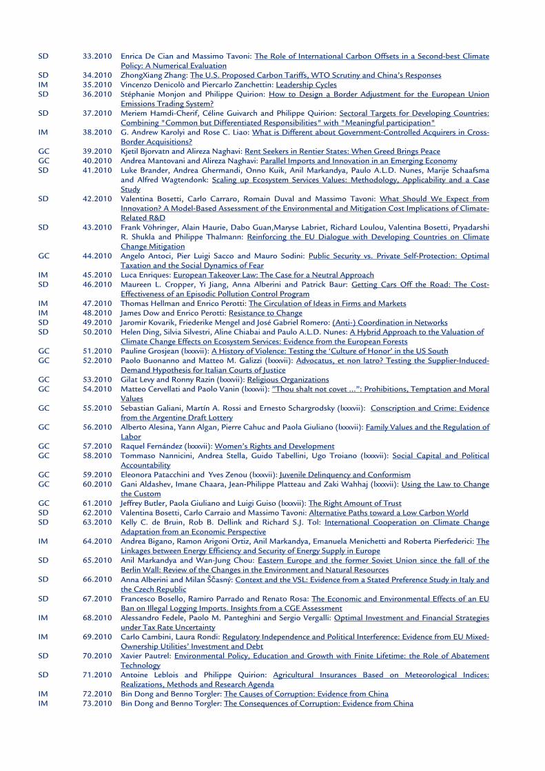
SD 33.2010 Enrica De Cian and Massimo Tavoni: The Role of International Carbon Offsets in a Second-best Climate Policy: A Numerical Evaluation
SD 34.2010 ZhongXiang Zhang: The U.S. Proposed Carbon Tariffs, WTO Scrutiny and China’s Responses IM 35.2010 Vincenzo Denicolò and Piercarlo Zanchettin: Leadership Cycles SD 36.2010 Stéphanie Monjon and Philippe Quirion: How to Design a Border Adjustment for the European Union
Emissions Trading System? SD 37.2010 Meriem Hamdi-Cherif, Céline Guivarch and Philippe Quirion: Sectoral Targets for Developing Countries:
Combining "Common but Differentiated Responsibilities" with "Meaningful participation" IM 38.2010 G. Andrew Karolyi and Rose C. Liao: What is Different about Government-Controlled Acquirers in Cross-
Border Acquisitions? GC 39.2010 Kjetil Bjorvatn and Alireza Naghavi: Rent Seekers in Rentier States: When Greed Brings Peace GC 40.2010 Andrea Mantovani and Alireza Naghavi: Parallel Imports and Innovation in an Emerging Economy SD 41.2010 Luke Brander, Andrea Ghermandi, Onno Kuik, Anil Markandya, Paulo A.L.D. Nunes, Marije Schaafsma
and Alfred Wagtendonk: Scaling up Ecosystem Services Values: Methodology, Applicability and a Case Study
SD 42.2010 Valentina Bosetti, Carlo Carraro, Romain Duval and Massimo Tavoni: What Should We Expect from Innovation? A Model-Based Assessment of the Environmental and Mitigation Cost Implications of Climate-Related R&D
SD 43.2010 Frank Vöhringer, Alain Haurie, Dabo Guan,Maryse Labriet, Richard Loulou, Valentina Bosetti, Pryadarshi R. Shukla and Philippe Thalmann: Reinforcing the EU Dialogue with Developing Countries on Climate Change Mitigation
GC 44.2010 Angelo Antoci, Pier Luigi Sacco and Mauro Sodini: Public Security vs. Private Self-Protection: Optimal Taxation and the Social Dynamics of Fear
IM 45.2010 Luca Enriques: European Takeover Law: The Case for a Neutral Approach SD 46.2010 Maureen L. Cropper, Yi Jiang, Anna Alberini and Patrick Baur: Getting Cars Off the Road: The Cost-
Effectiveness of an Episodic Pollution Control Program IM 47.2010 Thomas Hellman and Enrico Perotti: The Circulation of Ideas in Firms and Markets IM 48.2010 James Dow and Enrico Perotti: Resistance to Change SD 49.2010 Jaromir Kovarik, Friederike Mengel and José Gabriel Romero: (Anti-) Coordination in Networks SD 50.2010 Helen Ding, Silvia Silvestri, Aline Chiabai and Paulo A.L.D. Nunes: A Hybrid Approach to the Valuation of
Climate Change Effects on Ecosystem Services: Evidence from the European Forests GC 51.2010 Pauline Grosjean (lxxxvii): A History of Violence: Testing the ‘Culture of Honor’ in the US South GC 52.2010 Paolo Buonanno and Matteo M. Galizzi (lxxxvii): Advocatus, et non latro? Testing the Supplier-Induced-
Demand Hypothesis for Italian Courts of Justice GC 53.2010 Gilat Levy and Ronny Razin (lxxxvii): Religious Organizations GC 54.2010 Matteo Cervellati and Paolo Vanin (lxxxvii): ”Thou shalt not covet ...”: Prohibitions, Temptation and Moral
Values GC 55.2010 Sebastian Galiani, Martín A. Rossi and Ernesto Schargrodsky (lxxxvii): Conscription and Crime: Evidence
from the Argentine Draft Lottery GC 56.2010 Alberto Alesina, Yann Algan, Pierre Cahuc and Paola Giuliano (lxxxvii): Family Values and the Regulation of
Labor GC 57.2010 Raquel Fernández (lxxxvii): Women’s Rights and Development GC 58.2010 Tommaso Nannicini, Andrea Stella, Guido Tabellini, Ugo Troiano (lxxxvii): Social Capital and Political
Accountability GC 59.2010 Eleonora Patacchini and Yves Zenou (lxxxvii): Juvenile Delinquency and Conformism GC 60.2010 Gani Aldashev, Imane Chaara, Jean-Philippe Platteau and Zaki Wahhaj (lxxxvii): Using the Law to Change
the Custom GC 61.2010 Jeffrey Butler, Paola Giuliano and Luigi Guiso (lxxxvii): The Right Amount of Trust SD 62.2010 Valentina Bosetti, Carlo Carraio and Massimo Tavoni: Alternative Paths toward a Low Carbon World SD 63.2010 Kelly C. de Bruin, Rob B. Dellink and Richard S.J. Tol: International Cooperation on Climate Change
Adaptation from an Economic Perspective IM 64.2010 Andrea Bigano, Ramon Arigoni Ortiz, Anil Markandya, Emanuela Menichetti and Roberta Pierfederici: The
Linkages between Energy Efficiency and Security of Energy Supply in Europe SD 65.2010 Anil Markandya and Wan-Jung Chou: Eastern Europe and the former Soviet Union since the fall of the
Berlin Wall: Review of the Changes in the Environment and Natural Resources SD 66.2010 Anna Alberini and Milan Ščasný: Context and the VSL: Evidence from a Stated Preference Study in Italy and
the Czech Republic SD 67.2010 Francesco Bosello, Ramiro Parrado and Renato Rosa: The Economic and Environmental Effects of an EU
Ban on Illegal Logging Imports. Insights from a CGE Assessment IM 68.2010 Alessandro Fedele, Paolo M. Panteghini and Sergio Vergalli: Optimal Investment and Financial Strategies
under Tax Rate Uncertainty IM 69.2010 Carlo Cambini, Laura Rondi: Regulatory Independence and Political Interference: Evidence from EU Mixed-
Ownership Utilities’ Investment and Debt SD 70.2010 Xavier Pautrel: Environmental Policy, Education and Growth with Finite Lifetime: the Role of Abatement
Technology SD 71.2010 Antoine Leblois and Philippe Quirion: Agricultural Insurances Based on Meteorological Indices:
Realizations, Methods and Research Agenda IM 72.2010 Bin Dong and Benno Torgler: The Causes of Corruption: Evidence from China IM 73.2010 Bin Dong and Benno Torgler: The Consequences of Corruption: Evidence from China
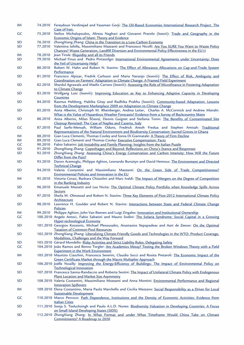
IM 74.2010 Fereydoun Verdinejad and Yasaman Gorji: The Oil-Based Economies International Research Project. The Case of Iran.
GC 75.2010 Stelios Michalopoulos, Alireza Naghavi and Giovanni Prarolo (lxxxvii): Trade and Geography in the Economic Origins of Islam: Theory and Evidence
SD 76.2010 ZhongXiang Zhang: China in the Transition to a Low-Carbon Economy SD 77.2010 Valentina Iafolla, Massimiliano Mazzanti and Francesco Nicolli: Are You SURE You Want to Waste Policy
Chances? Waste Generation, Landfill Diversion and Environmental Policy Effectiveness in the EU15 IM 78.2010 Jean Tirole: Illiquidity and all its Friends SD 79.2010 Michael Finus and Pedro Pintassilgo: International Environmental Agreements under Uncertainty: Does
the Veil of Uncertainty Help? SD 80.2010 Robert W. Hahn and Robert N. Stavins: The Effect of Allowance Allocations on Cap-and-Trade System
Performance SD 81.2010 Francisco Alpizar, Fredrik Carlsson and Maria Naranjo (lxxxviii): The Effect of Risk, Ambiguity and
Coordination on Farmers’ Adaptation to Climate Change: A Framed Field Experiment SD 82.2010 Shardul Agrawala and Maëlis Carraro (lxxxviii): Assessing the Role of Microfinance in Fostering Adaptation
to Climate Change SD 83.2010 Wolfgang Lutz (lxxxviii): Improving Education as Key to Enhancing Adaptive Capacity in Developing
Countries SD 84.2010 Rasmus Heltberg, Habiba Gitay and Radhika Prabhu (lxxxviii): Community-based Adaptation: Lessons
from the Development Marketplace 2009 on Adaptation to Climate Change SD 85.2010 Anna Alberini, Christoph M. Rheinberger, Andrea Leiter, Charles A. McCormick and Andrew Mizrahi:
What is the Value of Hazardous Weather Forecasts? Evidence from a Survey of Backcountry Skiers SD 86.2010 Anna Alberini, Milan Ščasný, Dennis Guignet and Stefania Tonin: The Benefits of Contaminated Site
Cleanup Revisited: The Case of Naples and Caserta, Italy GC 87.2010 Paul Sarfo-Mensah, William Oduro, Fredrick Antoh Fredua and Stephen Amisah: Traditional
Representations of the Natural Environment and Biodiversity Conservation: Sacred Groves in Ghana IM 88.2010 Gian Luca Clementi, Thomas Cooley and Sonia Di Giannatale: A Theory of Firm Decline IM 89.2010 Gian Luca Clementi and Thomas Cooley: Executive Compensation: Facts GC 90.2010 Fabio Sabatini: Job Instability and Family Planning: Insights from the Italian Puzzle SD 91.2010 ZhongXiang Zhang: Copenhagen and Beyond: Reflections on China’s Stance and Responses SD 92.2010 ZhongXiang Zhang: Assessing China’s Energy Conservation and Carbon Intensity: How Will the Future
Differ from the Past? SD 93.2010 Daron Acemoglu, Philippe Aghion, Leonardo Bursztyn and David Hemous: The Environment and Directed
Technical Change SD 94.2010 Valeria Costantini and Massimiliano Mazzanti: On the Green Side of Trade Competitiveness?
Environmental Policies and Innovation in the EU IM 95.2010 Vittoria Cerasi, Barbara Chizzolini and Marc Ivaldi: The Impact of Mergers on the Degree of Competition
in the Banking Industry SD 96.2010 Emanuele Massetti and Lea Nicita: The Optimal Climate Policy Portfolio when Knowledge Spills Across
Sectors SD
97.2010 Sheila M. Olmstead and Robert N. Stavins: Three Key Elements of Post-2012 International Climate Policy Architecture
SD 98.2010 Lawrence H. Goulder and Robert N. Stavins: Interactions between State and Federal Climate Change Policies
IM 99.2010 Philippe Aghion, John Van Reenen and Luigi Zingales: Innovation and Institutional Ownership GC 100.2010 Angelo Antoci, Fabio Sabatini and Mauro Sodini: The Solaria Syndrome: Social Capital in a Growing
Hyper-technological Economy SD 101.2010 Georgios Kossioris, Michael Plexousakis, Anastasios Xepapadeas and Aart de Zeeuw: On the Optimal
Taxation of Common-Pool Resources SD 102.2010 ZhongXiang Zhang: Liberalizing Climate-Friendly Goods and Technologies in the WTO: Product Coverage,
Modalities, Challenges and the Way Forward SD 103.2010 Gérard Mondello: Risky Activities and Strict Liability Rules: Delegating Safety GC 104.2010 João Ramos and Benno Torgler: Are Academics Messy? Testing the Broken Windows Theory with a Field
Experiment in the Work Environment IM 105.2010 Maurizio Ciaschini, Francesca Severini, Claudio Socci and Rosita Pretaroli: The Economic Impact of the
Green Certificate Market through the Macro Multiplier Approach SD 106.2010 Joëlle Noailly: Improving the Energy-Efficiency of Buildings: The Impact of Environmental Policy on
Technological Innovation SD 107.2010 Francesca Sanna-Randaccio and Roberta Sestini: The Impact of Unilateral Climate Policy with Endogenous
Plant Location and Market Size Asymmetry SD 108.2010 Valeria Costantini, Massimiliano Mozzanti and Anna Montini: Environmental Performance and Regional
Innovation Spillovers IM 109.2010 Elena Costantino, Maria Paola Marchello and Cecilia Mezzano: Social Responsibility as a Driver for Local
Sustainable Development GC 110.2010 Marco Percoco: Path Dependence, Institutions and the Density of Economic Activities: Evidence from
Italian Cities SD 111.2010 Sonja S. Teelucksingh and Paulo A.L.D. Nunes: Biodiversity Valuation in Developing Countries: A Focus
on Small Island Developing States (SIDS) SD 112.2010 ZhongXiang Zhang: In What Format and under What Timeframe Would China Take on Climate
Commitments? A Roadmap to 2050
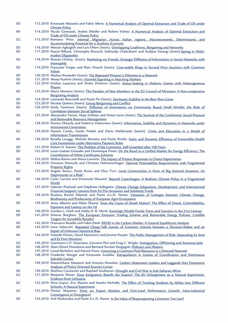
SD 113.2010 Emanuele Massetti and Fabio Sferra: A Numerical Analysis of Optimal Extraction and Trade of Oil under Climate Policy
IM 114.2010 Nicola Gennaioli, Andrei Shleifer and Robert Vishny: A Numerical Analysis of Optimal Extraction and Trade of Oil under Climate Policy
GC 115.2010 Romano Piras: Internal Migration Across Italian regions: Macroeconomic Determinants and Accommodating Potential for a Dualistic Economy
SD 116.2010 Messan Agbaglah and Lars Ehlers (lxxxix): Overlapping Coalitions, Bargaining and Networks SD 117.2010 Pascal Billand, Christophe Bravard, Subhadip Chakrabarti and Sudipta Sarangi (lxxxix):Spying in Multi-
market Oligopolies SD 118.2010 Roman Chuhay (lxxxix): Marketing via Friends: Strategic Diffusion of Information in Social Networks with
Homophily SD 119.2010 Françoise Forges and Ram Orzach (lxxxix): Core-stable Rings in Second Price Auctions with Common
Values SD 120.2010 Markus Kinateder (lxxxix): The Repeated Prisoner’s Dilemma in a Network SD 121.2010 Alexey Kushnir (lxxxix): Harmful Signaling in Matching Markets SD 122.2010 Emiliya Lazarova and Dinko Dimitrov (lxxxix): Status-Seeking in Hedonic Games with Heterogeneous
Players SD 123.2010 Maria Montero (lxxxix): The Paradox of New Members in the EU Council of Ministers: A Non-cooperative
Bargaining Analysis SD 124.2010 Leonardo Boncinelli and Paolo Pin (lxxxix): Stochastic Stability in the Best Shot Game SD 125.2010 Nicolas Quérou (lxxxix): Group Bargaining and Conflict SD 126.2010 Emily Tanimura (lxxxix): Diffusion of Innovations on Community Based Small Worlds: the Role of
Correlation between Social Spheres SD 127.2010 Alessandro Tavoni, Maja Schlüter and Simon Levin (lxxxix): The Survival of the Conformist: Social Pressure
and Renewable Resource Management SD 128.2010 Norma Olaizola and Federico Valenciano (lxxxix): Information, Stability and Dynamics in Networks under
Institutional Constraints GC 129.2010 Darwin Cortés, Guido Friebel and Darío Maldonado (lxxxvii): Crime and Education in a Model of
Information Transmission IM 130.2010 Rosella Levaggi, Michele Moretto and Paolo Pertile: Static and Dynamic Efficiency of Irreversible Health
Care Investments under Alternative Payment Rules SD 131.2010 Robert N. Stavins: The Problem of the Commons: Still Unsettled after 100 Years SD 132.2010 Louis-Gaëtan Giraudet and Dominique Finon: On the Road to a Unified Market for Energy Efficiency: The
Contribution of White Certificates Schemes SD 133.2010 Melina Barrio and Maria Loureiro: The Impact of Protest Responses in Choice Experiments IM 134.2010 Vincenzo Denicolò and Christine Halmenschlager: Optimal Patentability Requirements with Fragmented
Property Rights GC 135.2010 Angelo Antoci, Paolo Russu and Elisa Ticci: Local Communities in front of Big External Investors: An
Opportunity or a Risk? SD 136.2010 Carlo Carraro and Emanuele Massetti: Beyond Copenhagen: A Realistic Climate Policy in a Fragmented
World SD 137.2010 Valentin Przyluski and Stéphane Hallegatte: Climate Change Adaptation, Development, and International
Financial Support: Lessons from EU Pre-Accession and Solidarity Funds SD 138.2010 Ruslana Rachel Palatnik and Paulo A.L.D. Nunes: Valuation of Linkages between Climate Change,
Biodiversity and Productivity of European Agro-Ecosystems SD 139.2010 Anna Alberini and Milan Ščasný: Does the Cause of Death Matter? The Effect of Dread, Controllability,
Exposure and Latency on the Vsl IM 140.2010 Gordon L. Clark and Ashby H. B. Monk: Sovereign Wealth Funds: Form and Function in the 21st Century SD 141,2010 Simone Borghesi: The European Emission Trading Scheme and Renewable Energy Policies: Credible
Targets for Incredible Results? SD 142.2010 Francesco Bosello and Fabio Eboli: REDD in the Carbon Market: A General Equilibrium Analysis SD 143.2010 Irene Valsecchi: Repeated Cheap-Talk Games of Common Interest between a Decision-Maker and an
Expert of Unknown Statistical Bias IM 144.2010 Yolande Hiriart, David Martimort and Jerome Pouyet: The Public Management of Risk: Separating Ex Ante
and Ex Post Monitors GC 145.2010 Gianmarco I.P. Ottaviano, Giovanni Peri and Greg C. Wright: Immigration, Offshoring and American Jobs SD 146.2010 Alain-Désiré Nimubona and Bernard Sinclair-Desgagné: Polluters and Abaters SD 147.2010 Lionel Richefort and Patrick Point: Governing a Common-Pool Resource in a Directed Network SD 148.2010 Friederike Mengel and Emanuela Sciubba: Extrapolation in Games of Coordination and Dominance
Solvable Games SD 149.2010 Massimiliano Mazzanti and Antonio Musolesi: Carbon Abatement Leaders and Laggards Non Parametric
Analyses of Policy Oriented Kuznets Curves SD 150.2010 Mathieu Couttenier and Raphael Soubeyran: Drought and Civil War in Sub-Saharan Africa GC 151.2010 Benjamin Elsner: Does Emigration Benefit the Stayers? The EU Enlargement as a Natural Experiment.
Evidence from Lithuania GC 152.2010 Nina Guyon, Eric Maurin and Sandra McNally: The Effect of Tracking Students by Ability into Different
Schools: A Natural Experiment GC 153.2010 Florian Mayneris: Entry on Export Markets and Firm-Level Performance Growth: Intra-Industrial
Convergence or Divergence? SD 154.2010 Anil Markandya and Paulo A.L.D. Nunes: Is the Value of Bioprospecting Contracts Too Low?
SD 155.2010 William Brock and Anastasios Xepapadeas: Robust Control and Hot Spots in Dynamic SpatiallyInterconnected Systems
SD 156.2010 Johannes Herold, Sophia Rüster and Christian Von Hirschhausen: Carbon Capture; Transport and Storage in Europe: A Problematic Energy Bridge to Nowhere?
SD 157.2010 Valentina Giannini: REDD and International Organizations SD 158.2010 ZhongXiang Zhang: Assessing China’s Carbon Intensity Pledge for 2020: Stringency and Credibility Issues
and their Implications SD 159.2010 Francesco Bosello and Chen Chen: Adapting and Mitigating to Climate Change: Balancing the Choice
under Uncertainty (lxxxvi) This paper was presented at the Conference on "Urban and Regional Economics" organised by the Centre for Economic Policy Research (CEPR) and FEEM, held in Milan on 12-13 October 2009.
(lxxxvii) This paper was presented at the Conference on “Economics of Culture, Institutions and Crime” organised by SUS.DIV, FEEM, University of Padua and CEPR, held in Milan on 20-22 January 2010.
(lxxxviii) This paper was presented at the International Workshop on “The Social Dimension of Adaptation to Climate Change”, jointly organized by the International Center for Climate Governance, Centro Euro-Mediterraneo per i Cambiamenti Climatici and Fondazione Eni Enrico Mattei, held in Venice, 18-19 February 2010.
(lxxxix) This paper was presented at the 15th Coalition Theory Network Workshop organised by the Groupement de Recherche en Economie Quantitative d’Aix-Marseille, (GREQAM), held in Marseille, France, on June 17-18, 2010.
Related Documents