An enhanced XCS rule discovery module using feature ranking

1 23

International Journal of MachineLearning and Cybernetics ISSN 1868-8071Volume 4Number 3 Int. J. Mach. Learn. & Cyber. (2013)4:173-187DOI 10.1007/s13042-012-0085-9

An enhanced XCS rule discovery moduleusing feature ranking

Mani Abedini & Michael Kirley

1 23

Your article is protected by copyright and

all rights are held exclusively by Springer-

Verlag. This e-offprint is for personal use only

and shall not be self-archived in electronic

repositories. If you wish to self-archive your

article, please use the accepted manuscript

version for posting on your own website. You

may further deposit the accepted manuscript

version in any repository, provided it is only

made publicly available 12 months after

official publication or later and provided

acknowledgement is given to the original

source of publication and a link is inserted

to the published article on Springer's

website. The link must be accompanied by

the following text: "The final publication is

available at link.springer.com”.

ORIGINAL ARTICLE

An enhanced XCS rule discovery module using feature ranking

Mani Abedini • Michael Kirley

Received: 28 October 2011 / Accepted: 16 February 2012 / Published online: 18 March 2012

� Springer-Verlag 2012

Abstract XCS is a genetics-based machine learning

model that combines reinforcement learning with evolu-

tionary algorithms to evolve a population of classifiers in

the form of condition-action rules. Like many other

machine learning algorithms, XCS is less effective on high-

dimensional data sets. In this paper, we describe a new

guided rule discovery mechanisms for XCS, inspired by

feature selection techniques commonly used in machine

learning. In our approach, feature quality information is

used to bias the evolutionary operators. A comprehensive

set of experiments is used to investigate how the number of

features used to bias the evolutionary operators, population

size, and feature ranking technique, affect model perfor-

mance. Numerical simulations have shown that our guided

rule discovery mechanism improves the performance

of XCS in terms of accuracy, execution time and more

generally in terms of classifier diversity in the population,

especially for high-dimensional classification problems.

We present a detailed discussion of the effects of model

parameters and recommend settings for large scale

problems.

Keywords Learning classifier systems �Genetics-based machine learning � XCS � Feature ranking �High-dimensional classification � Microarray gene

expression profiles

1 Introduction

Classification problems arise frequently in many areas of

science and engineering. Examples include: disease

classification based on gene expression profiles in bio-

informatics; document classification in information

retrieval; image recognition; and fraud detection [32].

The goal of any classification algorithm, is to build a

model that captures the intrinsic associations between the

class type and the features (attributes) in an attempt to

match each input value to one of a given set of class

labels [28].

Learning classifier systems (LCS) are a type of genetics-

based machine learning (GBML) algorithm for rule

induction, which have been applied to a large variety of

classification problems [14, 23, 27]. LCS combine rein-

forcement learning with evolutionary computing and other

heuristics to produce an adaptive system that learns to

solve a particular problem. Of the Michigan-style GBML

methods, XCS [13, 34, 35] is perhaps the most well-known

architecture. Each individual in the XCS population

encapsulates a single rule (condition-action-prediction)

with an associated fitness value. Through an iterative

learning process, the population of classifiers evolves. A

key step in this iterative process is the rule discovery

component that creates new classifiers to be added to the

bounded population pool.

Over the last few years, the analysis of high-dimensional

data sets has been the subject of numerous publications in

statistics, machine learning, and bioinformatics. Consider a

prototypical high-dimensional data set, such as a micro-

array gene expression data set, that has several thousands

genes (features) but only a small number of samples.

Typically many of the features are irrelevant to the clas-

sification task [37]. Given the high-dimensional search

M. Abedini (&) � M. Kirley

Department of Computing and Information Systems,

The University of Melbourne, Victoria, Australia

e-mail: [email protected]

M. Kirley

e-mail: [email protected]

123

Int. J. Mach. Learn. & Cyber. (2013) 4:173–187

DOI 10.1007/s13042-012-0085-9

Author's personal copy

space, building effective classification models is a non-

trivial task for microarray gene expression data sets.

Standard XCS implementations, and many other

machine learning classification algorithms, are typically

less effective on data sets characterized by a high-dimen-

sional space—the curse of dimensionality. It is difficult to

effectively explore the solution space and build an appro-

priate classification model. There has only been a small

number of studies investigating XCS for high-dimensional

classification tasks that have appeared in the literature.

Representative examples include a study of large multi-

plexer problems [4] and more generally, work examining

the scalability of XCS [31]. In contrast, Pittsburg-style

GBML implementations have been used to classify large-

scale bioinformatics data sets (e.g. [8, 9]). In this approach,

each individual in the evolving population represents a

complete classification rule. As such, the evolved rules for

the high-dimensional data sets are typically very large.

Consequently, specialized evolutionary operators are

required to guide the learning process.

In this paper, a new guided rule discovery mechanisms

is proposed for XCS for high-dimensional classification

problems.1 Our model, called GRD-XCS, is inspired by

feature selection techniques commonly used in machine

learning. Typically, filtering techniques assess the rele-

vance of features in the data set. A subset of the ‘‘more

important’’ features is then presented as input to the clas-

sification algorithm while the ‘‘less important’’ features are

ignored. However, in our model the filtering process is

used to build a probability distribution that biases the

evolutionary operators encapsulated in the rule discovery

component of XCS. This probability distribution can be

thought of as a mask that biases the uniform crossover and

mutation operators. This flexible approach is scalable, and

the enhanced XCS can be used to tackle high-dimensional

classification tasks without reducing the dimensionality of

the data set.

The remainder of this paper is organized as follows. In

Sect. 2, the XCS model is described and an overview of the

role of feature ranking in machine learning is presented.

Related work focussed on GMBL evolutionary operators is

presented in Sect. 3. The GRD-XCS model is presented in

Sect. 4. In Sect. 5, the experimental methodology is

described and parameters listed. Experiment results are

presented in Sect. 6. Section 7 describes the effects of

alternative feature ranking techniques in the GRD-XCS

model. Finally, in Sect. 8 we summarize the findings of this

study and recommend parameter settings for complex,

large-scale classification problems. Avenues for future

work are also presented.

2 Background

2.1 XCS: the eXtended classifier system

In this subsection, we provide a brief overview of the

functionality of the XCS model. A more detailed discussion

of GBML classifier systems can be found in [14, 23, 27].

As an instance of a GBML algorithm, XCS represents

the knowledge extracted from a given problem as a pop-

ulation of evolving condition-action-prediction rules [34].

At each iteration of the model, these rules are evaluated.

Reinforcement learning and a search algorithm are then

used to evolve the population of classifiers (rules). The

three key components of the model are the representation

scheme used to encode the population of classifiers, the

credit assignment mechanism and the rule discovery. These

components are described below.

Each individual in the XCS population is a classifier that

maps input vectors to output signals (or class labels).

A suitable representation scheme is required for this

mapping. Originally, each feature in the vector (condition

part of the rule) was encoded using a ternary alphabet

{0, 1, #}, where # represents a ‘‘don’t care’’ feature.

Wilson [35] proposed an alternative real-value encoding

style for the feature vector that is now widely used. The

predicted class label (condition part of the rule) for a binary

problem can be encoded using a binary alphabet {0,1}. For

multi-class problems, larger alphabets can be used.

Given the population sizes typically used in GBML, it is

reasonable to expect that there will be many copies of the

same classifier in the population at any given point in time.

Consequently, the term macro classifier is used to describe

unique instances of classifiers in the population. Each macro

classifier has a numerosity value that counts the number of

identical macro classifier instances in the population. As

such, the number of macro classifiers in the population is a

measure of population diversity. From a programming and

implementation point of view, key processing steps are

performed using the macro classifiers, which significantly

improves the execution time of the model.

1 GRD-XCS was introduced in [5]. This paper is a revised and a

substantially extended version of that paper.

174 Int. J. Mach. Learn. & Cyber. (2013) 4:173–187

123


At each time step, the classifier system receives a

problem instance in the form of a vector of features. A

decision, that is, an action to be performed next based on

the input vector, must be determined. A match set [M] is

created consisting of rules (classifiers) that can be ‘‘trig-

gered’’ by the given data instance. A covering operator is

used to create new matching classifiers when [M] is empty.

A prediction array [PA] is calculated for [M] that contains

an estimation of the corresponding rewards for each of the

possible actions. Based on the values in the prediction

array, an action act is selected. Classifiers that support the

predicted action make up the Action Set [A] (see

Algorithm 1).

In response to act, the reinforcement mechanism is

invoked and the prediction p, prediction error �; accuracy

k, and fitness F of the classifiers are updated. The corre-

sponding numerical reward is distributed to the rules

accountable for it, thus improving the estimates of the

action values. The prediction and prediction error are

updated as follows:

p pþ bðR� pÞ and � �þ bðjR� pj � �Þ

where b is the learning rate (0 \ b\ 1). The classifier

accuracy is calculated from the following equations:

k ¼ 1 if �\�0

að ��0Þ�m

otherwise

�and k0 ¼ kP

x2½A� kx

Finally, the classifier fitness F is updated using the relative

accuracy value:

F F þ bðk0 � FÞ

In XCS, the classifier’s fitness value is updated based on

the accuracy of the actual reward prediction. This

accuracy-based fitness provides a mechanism for XCS to

build a complete action map of the input space.

Figure 1 provides a high-level overview of the classifi-

cation process using XCS. In this binary classification

example, the data features have real-values. Here, we show

one cycle of the ‘‘classification’’ steps: creating the mat-

ched set [M], prediction set [PA] and inferring the pre-

dicted label act.

The rule discovery module of XCS plays a very

important role. Typically, a genetic algorithm is responsi-

ble for improving the population of classifiers. During the

evolutionary learning process, fitness-proportionate selec-

tion is applied to [A]. Standard evolutionary operators,

uniform crossover and mutation, are then applied to the

selected individuals. In addition, a second mutation-style

operator—the don’t care operator—is used to randomly

modify a condition part of a classifier to the ‘‘don’t care’’

value #. The newly created offspring (classifiers) are then

added to the bounded population. A form of niching is then

used to determine if the offspring survive in the population

and/or which of the old members of the population are to

be deleted to make room for the new classifiers (offspring).

A subsumption mechanism combines similar classifiers and

a randomized deletion mechanism removes from the pop-

ulation classifiers with a low fitness.

2.2 Feature ranking

Our novel extension of the standard XCS framework is

based on feature ranking. Below we describe feature

ranking categories typically used in machine learning.

Specific techniques used in this study are discussed in more

detail in Sects. 4 and 7.

Feature (or attribute) selection is a term that describes a

range of machine learning and/or statistical techniques

used to select a subset of relevant features when building

robust learning models. Based on a nominated metric, the

ranking of particular features provides valuable informa-

tion about the relative ‘‘importance’’ of the features. It is

then assumed that the ‘‘top ranked’’ features are more

likely to be helpful for the classification task, rather than

Fig. 1 XCS model overview. The condition segment of the classifier

consists of a vector of features, each encoded using real or binary

values. The output signal (prediction class) is a binary value in this

case. The classifier’s fitness value is proportional to the accuracy of

the prediction of the reward. See text for further explanation

Int. J. Mach. Learn. & Cyber. (2013) 4:173–187 175

123


lower ranked features [19]. As such, feature selection/

ranking raises the possibility of reducing the negative

effect of the irrelevant features on a given learning task,

potentially speeding up the learning process significantly.

Feature ranking methods may be categorized into three

groups [19]: Filter, Wrapper and Embedded methods:

• Filter methods are independent of the learning process.

They typically use statistical information to rank

features. Common evaluation metrics include:

– Distance measure: based on the geometrical (or

Euclidean) distance between feature vectors.

– Information measure: based on entropy. Entropy is

a measure of information contents and allows

finding features which carry valuable information.

– Dependency measure: considers the dependency

between a feature and the class labels.

– Inconsistency measure: evaluate features with a

matched pattern, but different class labels.

• Wrapper methods represent a class of models that are

‘‘wrapped around’’ a classifier. They provide a feature

set to work with and collect valuable feedback related

to the learning process. These methods measure the

classification error and attempt to correct the feature

set. The most commonly used wrapper methods are:

Sequential Forward Selection and Sequential Backward

Selection.

• Embedded methods integrate the learning algorithm with

the feature ranking step. In this model, both algorithms

work tightly together to improve performance. For

instance, SVM/RFE uses Support Vector Machine

(SVM) ranking feature weights to eliminate the least

important feature each at each iteration of the model [16].

It is important to note, that our model uses ‘‘feature

quality’’ information to bias the rule discovery component

of XCS (detail in Sect. 4) In other words, our model uses a

feature ranking method to improve the accuracy and speed

of the learning, but does not remove any features from the

actual classification process.

3 Related work

It is well documented in the evolutionary computation

literature that the implementation of the genetic operators

can influence the trajectory of the evolving population.

However, there has been a paucity of studies focussed

specifically on the impact of selected evolutionary operator

implementations in LCS. We briefly discuss some of the

key studies related to XCS/LCS below.

In one of the first studies focussed on the rule discovery

component specifically for XCS, Butz et al. [11] have

shown that uniform crossover can ensure successful

learning in many tasks. In subsequent work, Butz et al. [12]

introduced an informed crossover operator, which extended

the usual uniform operator such that exchanges of effective

building blocks occurred. This approach helped to avoid

the over-generalization phenomena inherent in XCS [23].

In other work, Bacardit et al. [7] customized the GAssist

crossover operator to switch between the standard cross-

over or a new simple crossover, SX. The SX operator uses

a heuristic selection approach to take a minimum number

of rules from the parents (more than two), which can obtain

maximum accuracy. Morales-Ortigosa et al. [25] have also

proposed a new XCS crossover operator, BLX, which

allowed for the creation of multiple offspring with a

diversity parameter to control differences between off-

spring and parents. In a more comprehensive overview

paper, Morales-Ortigosa et al. [26] presented a systematic

experimental analysis of the rule discovery component in

LCS. Subsequently, they developed crossover operators to

enhance the discovery component based on evolution

strategies with significant performance improvements.

Other work focussed on biased evolutionary operators in

LCS include the work of Jos-Revuelta [21], who introduced a

hybridized GA-Tabu Search (GA-TS) method that employed

modified mutation and crossover operators. Here, the oper-

ator probabilities were tuned by analyzing all the fitness

values of individuals during the evolution process. Wang

et al. [33] used information gain as part of the fitness func-

tion in a GA. They reported improved results when com-

paring their model to other machine learning algorithms.

Recently, Huerta et al. [10] combined linear discriminant

analysis with a GA to evaluate the fitness of individuals and

associated discriminate coefficients for crossover and

mutation operators. Moore et al. [24] argued that the biasing

of the initial population, based on expert knowledge pre-

processing, should lead to improved the performance of the

evolutionary based model. In their approach, a statistical

method, Tuned ReliefF, was used to determine the depen-

dencies between features to seed the initial population. A

modified fitness function and a new guided mutation oper-

ator based on features dependency was also introduced,

leading to significantly improved performance.

4 Model

The motivation behind the design and development of the

GRD-XCS was to improve classifier performance espe-

cially for high-dimensional classification problems. Our

goal was to make the overall task computationally faster,

without degrading accuracy. To meet this goal, GRD-XCS

introduces a probabilistically guided rule discovery mech-

anism for XCS.


123


In GRD-XCS, information gathered from a nominated

feature ranking method is used to build a probability model

that biases the evolutionary mechanism of the XCS. The

feature ranking probability distribution values are recorded

in a Rule Discovery Probability vector (RDP). Each value

of the RDP vector ð2 ½0; 1:0�Þ is associated with a corre-

sponding feature. The RDP vector is then used to bias the

feature-wise uniform crossover, mutation, and don’t care

operators, which are part of the XCS rule discovery com-

ponent. The GRD-XCS framework is not restricted to one

specific feature ranking method. However, to clarify the

functionality of our model, and to illustrate how RDP

vector values can be calculated, we will use Information

Gain (IG) as the feature ranking method initially. In

Sect. 7, the effectiveness of a range of alternative feature

selection techniques will be examined.

The IG measure is defined as entropy reduction [20]:

IG ¼ HðCÞ � HðCjfiÞ ð1Þ

where H represent entropy, F = {f0, f1, …, fi, …, fn} is the

feature set, and C the classes in this context. Entropy is a

measure to quantify the information content, it is calculated

using the formula:

HðCÞ ¼Xj2C

pj log2 pj ð2Þ

where pj is the probability of having j in C, and the

conditional entropy is calculated as:

HðCjfiÞ ¼Xj2C

pj log2 HðCjfi ¼ jÞ ð3Þ

The actual values in the RDP vector are calculated based

on the IG values as described below:

RDPi ¼1�cX � ðX� iÞ þ c if i�X

n otherwise

�ð4Þ

where i represents the rank index in ascending order for the

selected top ranked features X: The probability values

associated with the other features are given a very low

value n. Thus, all features have a chance to participate in

the rule discovery process. However, the X-top ranked

features have a greater chance of being selected (see

Fig. 2).

GRD-XCS uses the probability values recorded in the

RDP vector in the pre-processing phase to bias the evolu-

tionary operators used in the rule discovery phase of XCS.

The modified algorithms describing the crossover, muta-

tion and don’t care operators in GRD-XCS are very similar

to standard XCS operators:

• GRD-XCS crossover operator: The crossover operator

is a hybrid uniform/n-point function. An additional

check of each feature is carried out before exchange of

genetic material. If rand() \ RDP[i] then feature i is

swapped between the selected parents.

• GRD-XCS mutation operator: Uses the RDP vector to

determine if feature i is to undergo a mutation, if the

feature was randomly selected to be mutated.

• GRD-XCS don’t care operator: In this special mutation

operator, the values in the RDP vector are used in the

reverse order. That is, if the feature i has been selected

to be mutated and rand() \ (1 - RDP[i]), then feature

i is changed to # (‘‘don’t care’’).

The application of the RDP vector reduces the cross-

over and mutation probabilities for ‘‘uninformative’’ fea-

tures. However, it increases the ‘‘don’t care’’ operator

probability for the same feature. Therefore, the more

informative features (based on the IG measure in this case)

should appear in rules more often than the ‘‘uninforma-

tive’’ ones.

5 Experiments

We have conducted a series of independent experiments to

verify if the guided rule discovery mechanism for XCS was

Fig. 2 Information Gain is used to rank the features. The top Xfeatures (in this example X ¼ 5) are selected and allocated relatively

large probability values 2 ½c; 1�: The RDP vector maintains these

values. The highest ranked feature value is set to 1.0. Other features

receive smaller values relative to their rank (in this example c = 0.5).

Features that are not selected based on information gain are assigned

very small probability values (in this example n = 0.1)


123


able to evolve accurate classifiers. In particular, we wished

to establish if our proposed model had statistically sig-

nificantly improved accuracy values when compared to the

standard XCS across a suite of benchmark classification

problems. Detailed analyses of the effects of GRD-XCS

parameter values and alternative feature ranking tech-

niques were performed to evaluate the efficacy of the

model.

5.1 Data sets

Eight different data sets—four low-dimensional data sets

and four high-dimensional data sets—have been used in the

experiments. The details of these data sets are reported in

Table 1. The low dimensional data sets were selected from

the UCI [2] machine learning repository. They are bench-

mark data sets and provide a base line to compare our

model with other machine learning methods.

Four DNA microarray gene expression data sets were

selected to represent the high-dimensional data sets. Gene

expression profiles provide important insights into, and

further our understanding of, biological processes. They

are key tools used in medical diagnosis, treatment, and

drug design [36]. From a clinical perspective, the classi-

fication of gene expression is an important problem and a

very active research area. DNA microarray technology

has advanced a great deal in recent years. It is possible to

simultaneously measure the expression levels of thou-

sands of genes under particular experimental environ-

ments and conditions [37]. However, the number of

samples tends to be a much smaller than the number of

genes (features). Consequently, the high dimensionality

of a given data set poses many statistical and analytical

challenges, often degrading the generality of the machine

learning methods.

5.2 Parameters

Two different parameter types must be considered in GRD-

XCS. These are parameters specific to the underlying XCS

model and parameters specific to the guided-rule discovery

component of GRD-XCS.

For the base-XCS parameters in our model, we have

used default values recommended in [13]. For the UCI low-

dimensional data sets, the population size pop_size was set

to 2,000 individuals. For the gene expression high-dimen-

sional data sets, a range of alternative population sizes

were investigated (pop_size=500, 1,000, 2,000, 5,000).

When calculating the RDP vector values, we have used

IG for all experiments described in Sect. 6. Alternative

feature selection techniques are used in Sect. 7. For the low

dimensional data sets, all features were considered. That is,

the number of top ranked features X was equal to the

number of features in the data set. For the high dimensional

data sets, a range of alternative top ranked features sizes

were investigated (X ¼ 32; 64; 128; 256). In Eq. 4, c = 0.5

and n = 0.1.

In all experiments the number of iterations was set to

5,000.

5.3 Implementation

GRD-XCS was implemented in C, based on the XCS code

available from [1]. The WEKA package (version 3.6.1) [3]

was used for feature ranking. WEKA implementations for

the alternative machine learning algorithms listed in

Sect. 6.4 were also used.

All experiments were performed on the VPAC2 Tango

Cluster server. Tango has 111 computing nodes. Each node

is equipped with two 2.3 GHz AMD based quad core

Opteron processors, 32GB of RAM and four 320GB hard

drives. Tango’s operating system is the Linux distribution

CentOS (version 5).

Statistical analysis was performed using the IBM SPSS

Statistics (version 19) software.

5.4 Evaluation

For each scenario (parameter values—data set combina-

tion), we performed N-fold cross validation experiments

over 100 trials (see Table 1). The average accuracy values

for specific parameter combinations have been reported

using the Area Under the ROC Curve—the AUC value.

The ROC curve is a graphical way to depict the tradeoff

between the True Positive rate (TPR) on the Y axis and the

False Positive rate (FPR) on the X axis. The AUC values

Table 1 Data set details

Data set #Instances #Features Cross

validation

References

Low-dimensional data sets (UCI examples)

Pima 768 8 10 [2]

WBC 699 9 10 [2]

Hepatits 155 19 10 [2]

Parkinson 197 23 10 [2]

High-dimensional data sets (Microarray DNA gene expression)

Breast cancer 22 3,226 3 [18]

Colon cancer 62 2,000 10 [6]

Leukemia

cancer

72 7,129 10 [15]

Prostate cancer 136 12,600 10 [30]2 Victorian Partnership for Advanced Computing: http://www.

vpac.org.


123


http://www.vpac.org

http://www.vpac.org

obtained from the ROC graphs allow for easy comparison

between two or more plots. Larger AUC values represent

higher overall accuracy.

Appropriate statistical analyses using paired t test and/or

analysis of variance (ANOVA) were conducted to deter-

mine whether there were statistically significant differences

between particular scenarios in terms of both accuracy and

execution times. Scatter plots of the observed and fitted

values and Q–Q plots were used to verify normality

assumptions.

6 Results

The experimental results using the IG feature ranking

technique have been divided up into four sections to

highlight key attributes of the GRD-XCS model. In

Sect. 6.1, an analysis of the accuracy (AUC) values is

presented for different population sizes and X values. In

Sect. 6.2, we analyze execution times for different pop-

ulation sizes and X values. In Sect. 6.3, the population

diversity, measured in terms of the number and length of

macro classifiers in the final population, is examined.

Finally, in Sect. 6.4, we compare the performance of

GRD-XCS with other well-known machine learning

classifiers.

6.1 Accuracy analysis

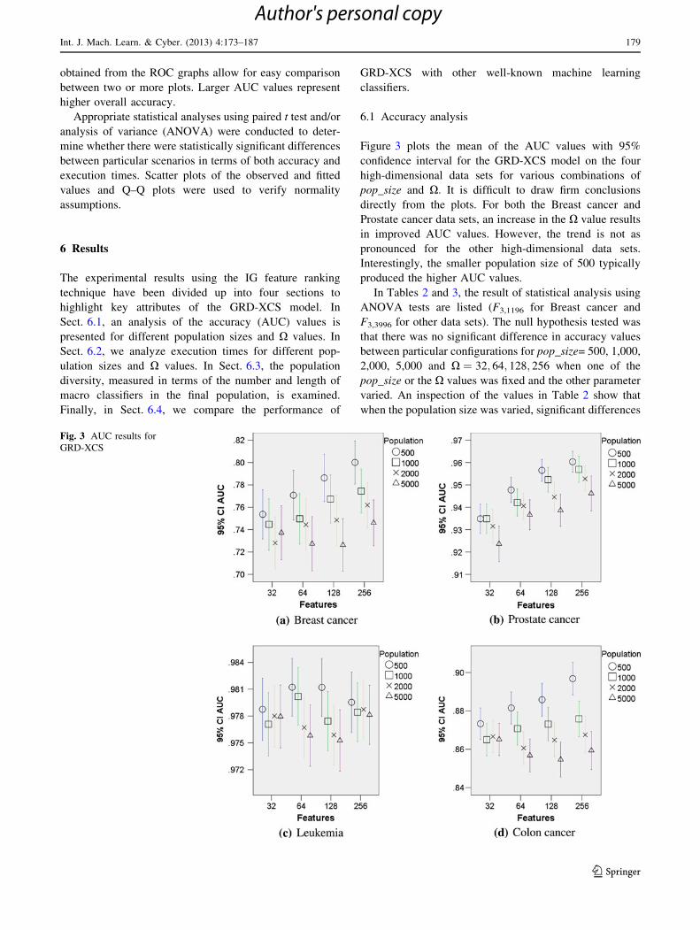
Figure 3 plots the mean of the AUC values with 95%

confidence interval for the GRD-XCS model on the four

high-dimensional data sets for various combinations of

pop_size and X: It is difficult to draw firm conclusions

directly from the plots. For both the Breast cancer and

Prostate cancer data sets, an increase in the X value results

in improved AUC values. However, the trend is not as

pronounced for the other high-dimensional data sets.

Interestingly, the smaller population size of 500 typically

produced the higher AUC values.

In Tables 2 and 3, the result of statistical analysis using

ANOVA tests are listed (F3,1196 for Breast cancer and

F3,3996 for other data sets). The null hypothesis tested was

that there was no significant difference in accuracy values

between particular configurations for pop_size= 500, 1,000,

2,000, 5,000 and X ¼ 32; 64; 128; 256 when one of the

pop_size or the X values was fixed and the other parameter

varied. An inspection of the values in Table 2 show that

when the population size was varied, significant differences

Fig. 3 AUC results for

GRD-XCS


123


existed between the accuracy values recorded when X ¼ 128

and higher for three of the data sets. Table 3 shows that

significant differences existed between the accuracy values

recorded for the small population size (500) for three of the

data sets when X was varied. A Tukey HSD post-hoc

comparison test suggests that for small changes in the con-

figuration (either pop_size or X), the accuracy levels of the

GRD-XCS are not significantly different. A linear regression

analysis reveals that the X parameter has a positive coeffi-

cient and the population size has a negative coefficient. Here,

the X coefficient is ten times larger than the other coefficient.

This suggests that smaller population sizes with relatively

larger X values should produce the best results. This obser-

vation is consistent with the plots in Fig. 3.

It is interesting to note that there were no significant

differences between configuration examined for the Leu-

kemia dataset. In the following sections, we will see that the

Leukemia data set is relatively easy to classify, not only by

GRD-XCS but also with other machine learning methods.

Therefore, changing the GRD-XCS configuration does not

have any significant effect on the accuracy values obtained.

6.2 Execution time analysis

The execution time of a GBML classifier system is a per-

formance metric that depends on many factors, including

the hardware specification, the number of records in the

data set, and the number of features in the data set. Here,

we restrict our analysis to a comparison of different GRD-

XCS parameters (population size and X) for each of the

data sets using the same hardware.

Figure 4 shows the average GRD-XCS model execution

time over 100 trials for each of the configurations exam-

ined. Error bars have been omitted for clarity. As expected,

an increase in the value of X and/or population size slows

the learning process down. This may be attributed to

increases in the execution time of the GetMatchSet()

function and the number of operations performed as part of

the rule discovery component (that is, as X increases in

value more features are involved in the crossover and

mutation operators). The large population size means that

there are more classifiers in the population to be processed

leading to an increase in execution time.

Statistical tests (ANOVA tests and Tukey HSD post-hoc

comparisons) show that execution time of all configuration

are significantly different (p \ 0.001). The regression

analysis for execution time indicates that the X coefficient

is ten times larger than the population size coefficient. If

the X values are not restricted to relatively small values,

execution time grows very fast. Based on this observation,

and the accuracy results listed in Sect. 6.1, a X of 128

appears to be a good choice for most high-dimensional data

sets.

6.3 Population diversity analysis

Population diversity is often seen as an important indicator

of evolutionary algorithm performance. Finding the right

balance between population diversity and convergence

speed is an on-going research challenge when confronted

with complex search and optimization problems. For GRD-

XCS, population diversity can be measure by the number

of unique classifiers—the macro classifiers—in the popu-

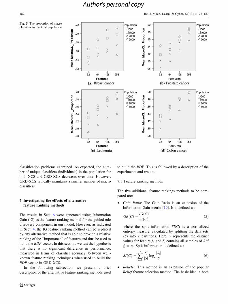
lation. Figure 5 plots the proportion of macro classifiers in

the final population averaged across 100 trials for different

scenarios. Errors bars have been omitted for clarity. As

expected, as the value of X increase the proportion of

macro classifiers, and thus population diversity, increases.

Population diversity tends to decrease based on this metric

for larger population sizes for fixed X values.

Given the role of the don’t care (#) feature encoding in

XCS, the length of the macro classifiers provides further

insights into algorithm performance. Figure 6 plots the

mean length (labelled as Mean Avg Att Size) of macro

classifiers in the final population averaged across 100 trials

for different scenarios. As the value of X increases, the

mean length of the macro classifiers increases. Generally,

an increase in the population size results in the evolution of

small macro classifiers, although this finding is not always

Table 2 ANOVA test results: X value is fixed—pop_size variable

Data set Top ranked features (X)

32 64 128 256

Breast cancer 0.465 0.073 0.001 0.002

Prostate cancer 0.102 0.075 \0.001 0.011

Leukemia 0.932 0.067 0.062 0.944

Colon cancer 0.465 \0.001 \0.001 \0.001

For example for the breast cancer data set, when X ¼ 32 there is no

significant difference (p = 0.465) between population sizes. In con-

trast, when X ¼ 128 the results are significantly different (p = 0.001)

Table 3 ANOVA test results: pop_size is fixed—X value variable

Data Set Population size (pop_size)

500 1,000 2,000 5,000

Breast cancer 0.017 0.176 0.214 0.600

Prostate cancer \0.001 \0.001 \0.001 0.001

Leukemia 0.664 0.573 0.735 0.885

Colon cancer 0.001 0.363 0.711 0.426

For example for the Breast cancer data set, when pop_size=500 there

is a significant difference (p = 0.017) between the X values. In

contrast, when pop_size=2000 there is no significant difference

(p = 0.214)


123


statistically significant across the high-dimensional data

sets.

One observation that can be made based on the plots is

that an increase the length of the macro classifiers does not

necessarily improve the accuracy, but it certainly will

increase the execution time.

6.4 Comparing GRD-XCS with other machine

learning techniques

In this subsection, the performance of the GRD-XCS

model in terms of accuracy is compared with a number of

well established machine learning methods. The WEKA

toolkit with default implementation was used to generate

results for these methods. The results for the GRD-XCS

were generated using a pop_size=500 and X ¼ 128: All

other parameters were default values listed in Sect. 5.2

Tables 4 and 5 list accuracy results for the low-dimen-

sional and high-dimensional respectively. The bold value

in each column indicates the highest mean accuracy value

over all trials. The dagger (�) symbol indicates that the

result for the classifier listed in the row was significantly

better than the GRD-XCS result based on a paired t test

(p \ 0.05).

For the low-dimensional data sets, the results show that

GRD-XCS is more accurate than standard XCS, although

this difference was not always statistically significant.

However, it is a different story when GRD-XCS is com-

pared to other machine learning methods. The performance

of GRD-XCS was best only for one data set, the Parkinson

data set.

In contrast, for the high-dimensional data sets the results

for GRD-XCS were significantly better than the other

machine learning methods based on paired t tests. A direct

comparison between GRD-XCS and the standard XCS

clearly illustrates that the guided rule discovery mechanism

leads to improved performance.

To further explore the efficacy of the our guided rule

discovery enhancements, Fig. 7 plots time series perfor-

mance values. Here, the overall accuracy and the number

of macro classifiers in the evolving population for both

the GRD-XCS and the standard XCS for representative

low-dimensional and high-dimensional data sets are pro-

vided. Space constraints preclude the inclusion of plots

for all data sets. However, the general trends for other

data sets are qualitatively similar. There is a correlation

between the accuracy of the model and the number of

macro-classifiers in the population for high-dimensional

Fig. 4 Execution time results

for GRD-XCS


123


classification problems examined. As expected, the num-

ber of unique classifiers (individuals) in the population for

both XCS and GRD-XCS decreases over time. However,

GRD-XCS typically maintains a smaller number of macro

classifiers.

7 Investigating the effects of alternative

feature ranking methods

The results in Sect. 6 were generated using Information

Gain (IG) as the feature ranking method for the guided rule

discovery component in our model. However, as indicated

in Sect. 4, the IG feature ranking method can be replaced

by any alternative method that is able to provide a relative

ranking of the ‘‘importance’’ of features and thus be used to

build the RDP vector. In this section, we test the hypothesis

that there is no significant difference in performance,

measured in terms of classifier accuracy, between well-

known feature ranking techniques when used to build the

RDP vector in GRD-XCS.

In the following subsection, we present a brief

description of the alternative feature ranking methods used

to build the RDP. This is followed by a description of the

experiments and results.

7.1 Feature ranking methods

The five additional feature rankings methods to be com-

pared are:

• Gain Ratio: The Gain Ratio is an extension of the

Information Gain metric [19]. It is defined as:

GRðCÞ ¼ IGðCÞSIðCÞ ð5Þ

where the split information SI(C) is a normalized

entropy measure, calculated by splitting the data sets

(S) into v partitions. Here, v represents the distinct

values for feature fi, and Si contains all samples of S if

fi = aj. Split information is defined as:

SIðCÞ ¼Xv

j¼1

jSijjSj log2

jSijjSj ð6Þ

• ReliefF: This method is an extension of the popular

Relief feature selection method. The basic idea in both

Fig. 5 The proportion of macro

classifier in the final population


123


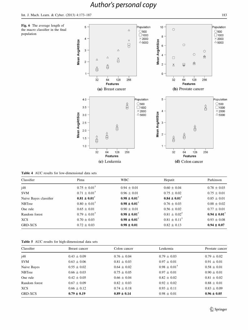
Fig. 6 The average length of

the macro classifier in the final

population

Table 4 AUC results for low-dimensional data sets

Classifier Pima WBC Hepatit Parkinson

j48 0.75 ± 0.01� 0.94 ± 0.01 0.60 ± 0.04 0.78 ± 0.03

SVM 0.71 ± 0.01� 0.96 ± 0.01 0.75 ± 0.02 0.75 ± 0.01

Naive Bayes classifier 0.81 – 0.01� 0.98 – 0.01� 0.84 – 0.01� 0.85 ± 0.01

NBTree 0.80 ± 0.01� 0.98 – 0.01� 0.76 ± 0.03 0.88 ± 0.02

One rule 0.65 ± 0.01 0.90 ± 0.01 0.56 ± 0.02 0.77 ± 0.01

Random forest 0.79 ± 0.01� 0.98 – 0.01� 0.81 ± 0.02� 0.94 – 0.01�

XCS 0.70 ± 0.03 0.98 – 0.01� 0.81 ± 0.11� 0.93 ± 0.08

GRD-XCS 0.72 ± 0.03 0.98 – 0.01 0.82 ± 0.13 0.94 – 0.07

Table 5 AUC results for high-dimensional data sets

Classifier Breast cancer Colon cancer Leukemia Prostate cancer

j48 0.43 ± 0.09 0.76 ± 0.04 0.79 ± 0.03 0.79 ± 0.02

SVM 0.63 ± 0.06 0.81 ± 0.03 0.97 ± 0.01 0.91 ± 0.01

Naive Bayes 0.55 ± 0.02 0.64 ± 0.02 0.98 ± 0.01� 0.58 ± 0.01

NBTree 0.66 ± 0.03 0.75 ± 0.05 0.97 ± 0.01 0.90 ± 0.01

One rule 0.42 ± 0.05 0.66 ± 0.04 0.82 ± 0.02 0.81 ± 0.02

Random forest 0.67 ± 0.09 0.82 ± 0.03 0.92 ± 0.02 0.88 ± 0.01

XCS 0.66 ± 0.12 0.74 ± 0.18 0.93 ± 0.11 0.83 ± 0.09

GRD-XCS 0.79 – 0.19 0.89 – 0.14 0.98 ± 0.01 0.96 – 0.05


123


algorithms is to adjust a weight vector for features,

thereby selecting random sample points and computing

their nearest neighbors. More weight is given to

features that discriminate samples from neighbors of

different class [22].

• Correlation based feature selection (CFS): CFS con-

sider both the relation between features and class, and

inter-correlation between features. The goal is to find a

subset of features that are highly correlated with the

predict the class label, as well as highly uncorrelated to

each others [17].

• Support Vector Machine feature selection: In this

approach, an SVM model is trained. Then in an

iterative fashion, features associated with small weights

are removed. The SVM is trained again with the

remaining features. This process continues until all

feature have been processed. A backward collecting

stage is then used to create the rank list [29].

• One Rule is a very simple, yet accurate, classification

method. This method is based on creating one rule for

each feature. Then, the error rates of each rule can be

used for ranking the features [19].

7.2 Experiments and result

Experiments were conducted to compare the accuracy

values found by GRD-XCS when each of the alternative

feature ranking methods was used. The GRD-XCS

parameter values used in the experiments were based on

the recommendation from Sect. 6: pop_size=500 and X ¼128: The remaining GRD-XCS parameters were set to

default values (see Sect. 5.2). The four high-dimensional

microarray gene expression data sets were used for com-

parisons purposes.

Detailed statistical tests were carried out to determine if

there were significant differences between the scenarios

considered. Table 6 lists the accuracy values obtained

averaged over 100 trials for each of the feature ranking

methods. The results of the ANOVA tests indicate

that feature ranking method used has a significant impact

on the accuracy values found using GRD-XCS for the

Breast cancer, Prostate cancer and Colon cancer data

sets (F5,1794 = 37.113 , p \ 0.0001; F5,5994 = 9.077 , p \0.0001; F5,5994 = 9.608 , p \ 0001 respectively). How-

ever, the results from the Leukemia data set (F5,1794 =

1.079 , p \ 0.370) were not significantly different. Given

the high accuracy levels obtained for the Leukemia data

set, simply by using a feature selection method it is rea-

sonable to expect an improvement in performance.

Tukey HSD post-hoc comparison tests were performed

for each scenario. For the Breast cancer data set, IG, CFS,

ReliefF, and SVM have similar performance levels

(p \ 0.05). The results also indicate that ReliefF, SVM,

and Gain Ratio have similar performance levels (p \ 0.05).

For the Prostate cancer data set, the only feature ranking

technique that was statistically significantly different to the

other techniques was the CFS method. The results of the

test for Colon data sets suggests that the six different fea-

ture ranking methods can be categorized into three subsets:

CFS and SVM as the first subset; SVM, Information Gain,

and ReliefF as the second subset and Information Gain,

ReliefF, Gain Ratio, and One Rule as the third subset.

This detailed statistical analysis suggests that the

effectiveness of the feature ranking method within the

GRD-XCS rule discovery component is somewhat

(a) (b)

Fig. 7 Time series performance plots for accuracy (left y-axis, blacklines) and the number of macro classifiers (right y-axis, blue lines) for

the a Parkinson (low-dimensional) and b breast cancer (high-

dimensional) data sets. Results for the base line XCS model (dottedline) and the GRD-XCS model (solid line) are provided (color figure

online)


123


dependent on the underlying characteristics of the data set.

There is no one specific feature ranking method that always

provides the best result. The use of any feature ranking

method generally leads to an improvement in the perfor-

mance of GRD-XCS when compared to the base-line XCS

model. In Table 6, each of the feature selection techniques

has been allocated a relative rank for each data set based on

the 95% confidence interval values. Across all data sets, IG

has the highest overall rank (1.5), followed by ReliefF,

SVM, One Rule, Gain Ratio, and CFS, respectively. A

reasonable conclusion, based on this analysis, is that IG is

an effective feature ranking method for GRD-XCS. IG is a

simple, informative approach that can be used to create the

probability model (the RDP vector) for biasing the evolu-

tionary operators in XCS.

8 Conclusion

In this paper, we have introduced a novel guided rule

discovery component for XCS specifically designed to

tackle high-dimensional classification problems. Here, a

filtering or feature ranking process is applied to build a

probabilistic model. This probability distribution is then

used to bias the evolutionary operators in the underlying

XCS model.

Comprehensive numerical simulations have shown that

our guided rule discovery mechanism improves the per-

formance of XCS in terms of accuracy, execution time and

more generally in terms of classifier diversity in the pop-

ulation. Detailed statistical analysis of the results suggests

that relatively small population sizes coupled with an

increasing number of top ranked features (X value) gen-

erally leads to high accuracy values. However, increased

execution time is a direct negative effect of increasing the

number of top features used in the RDP vector and/or the

population size. A comparative study of alternative feature

selection methods suggests that the use of any feature

selection technique, given the right parameter values, leads

to an improvement in performance. Clearly the quality of

the information extracted using any feature ranking method

is correlated with the underlying characteristics of the data

set. However, the use of any additional information to bias

the rule discovery evolutionary operators has been shown

to be useful. We conclude that the use of IG as the feature

selection method, with relatively small population sizes

and a small number of top ranked features in comparison to

the number of features in the data set, generally leads to the

Table 6 AUC feature ranking

methods resultsData set Method Mean of accuracy % 95 CI Rank

Breast cancer Information Gain 0.79 [0.77 0.81] 1

Gain Ratio 0.74 [0.72 0.76] 5

ReliefF 0.77 [0.75 0.79] 3

Correlation based 0.78 [0.76 0.80] 2

SVM 0.76 [0.74 0.78] 4

One rule 0.63 [0.61 0.64] 6

Prostate cancer Information Gain 0.96 [0.95 0.96] =2

Gain Ratio 0.95 [0.95 0.96] 3

ReliefF 0.97 [0.96 0.97] =1


SVM 0.97 [0.96 0.98] =1

One rule 0.96 [0.96 0.97] =2

Leukemia Information Gain 0.98 [0.98 0.98] =1

Gain Ratio 0.98 [0.98 0.98] =1

ReliefF 0.98 [0.98 0.99] =1

Correlation based 0.98 [0.98 0.99] =1

SVM 0.98 [0.97 0.99] =1

One rule 0.98 [0.97 0.98] =1

Colon cancer Information Gain 0.89 [0.88 0.89] =2

Gain Ratio 0.89 [0.89 0.90] =2

ReliefF 0.89 [0.88 0.90] =2


SVM 0.87 [0.86 0.88] 3

One rule 0.90 [0.89 0.91] 1


123


best accuracy values given constraints on computational

time.

There are many avenues to explore in future work. The

feature quality information extracted from a feature rank-

ing method could be further refined. For example, a cor-

relation detection method could be used to modify the RDP

values for correlated features. In addition, specific domain

knowledge (such as the identification of highly suspicious

genes in microarray gene expression data sets) could pro-

vide an alternative feature quality information for biasing

the evolutionary operators. There is also scope to investi-

gate ways to reduce execution time based on parallel

deployment of the GRD-XCS model.

References

1. The XCS source code in C is freely available on Illinois Genetic

Algorithms Laboratory (IlliGAL) web site: http://illigal.org/

category/source-code.

2. UCI Machine Learning Repository: The Center for Machine

Learning and Intelligent Systems at the University of California,

Irvine. http://archive.ics.uci.edu/ml

3. Weka 3, is an open source data mining tool (in java), with a

collection of machine learning algorithms developed by Machine

Learning Group at University of Waikato. http://www.cs.waikato.

ac.nz/ml/weka

4. Abedini M, Kirley M (2010) A multiple population XCS:

evolving condition-action rules based on feature space partitions.

In: 2010 IEEE Congress on Evolutionary computation (CEC),

pp 1–8, July 2010

5. Abedini M, Kirley M (2011) Guided rule discovery in XCS for

high-dimensional classification problems. In: Proceedings of 24th

Australasian artificial intelligence conference. Lecture notes in

artificial intelligence, vol 7106

6. Alon U, Barkai N, Notterman DA, Gishdagger K, Ybarradagger

S, Mackdagger D, Levine AJ (1999) Broad patterns of gene

expression revealed by clustering analysis of tumor and normal

colon tissues probed by oligonucleotide arrays. Proc Natl Acad

Sci USA 96:6745–6750

7. Bacardit J, Krasnogor N (2006) Smart crossover operator with

multiple parents for a Pittsburgh learning classifier system. In:

Proceedings of the 8th conference on GECCO. ACM, New York,

pp 1441–1448

8. Bacardit J, Stout M, Hirst JD, Sastry K, Lloraa X, Krasnogor N

(2007) Automated alphabet reduction method with evolutionary

algorithms for protein structure prediction. In: Thierens D, Beyer

H-G, Bongard J, Branke J, Clark JA, Cliff D, Congdon CB, Deb

K, Doerr B, Kovacs T, Kumar S, Miller JF, Moore J, Neumann F,

Pelikan M, Poli R, Sastry K, Stanley KO, Stutzle T, Watson RA,

Wegener I (eds) GECCO ’07: Proceedings of the 9th annual

conference on Genetic and evolutionary computation, vol 1,

London, 7–11 July 2007. ACM Press, New York, pp 346–353

9. Bacardit J, Stout M, Krasnogor N, Hirst JD, Blazewicz J (2006)

Coordination number prediction using learning classifier systems:

performance and interpretability. In: Cattolico M (ed) Genetic

and evolutionary computation conference, GECCO 2006, pro-

ceedings, Seattle, Washington, USA, July 8–12, 2006. ACM,

New York, pp 247–254

10. Bonilla Huerta E, Hernandez Hernandez J, Hernandez Montiel L

(2010) A new combined filter-wrapper framework for gene subset

selection with specialized genetic operators. In: Advances in

pattern recognition. Lecture notes in computer science, vol 6256.

Springer, Berlin/Heidelberg, pp 250–259

11. Butz MV, Goldberg DE, Tharakunnel K (2003) Analysis and

improvement of fitness exploitation in XCS: bounding models,

tournament selection, and bilateral accuracy. Evol Comput

11:239–277

12. Butz MV, Pelikan M, Lloraa X, Goldberg DE (2006) Automated

global structure extraction for effective local building block

processing in XCS. Evol Comput 14:345–380

13. Butz MV, Wilson SW (2001) An Algorithmic description of

XCS. In: Advances in learning classifier systems. Lecture notes in

computer science, vol 1996/2001. Springer, Berlin/Heidelberg,

pp 267–274

14. Fernandndez A, Garcianda S, Luengo J, Bernado-Mansilla E,

Herrera F (2010) Genetics-based machine learning for rule

induction: state of the art, taxonomy, and comparative study.

IEEE Trans Evol Comput 14(6):913–941

15. Golub TR, Slonim DK, Tamayo P, Huard C, Gaasenbeek M,

Mesirov JP, Coller H, Loh ML, Downing JR, Caligiuri MA,

Bloomfield CD (1999) Molecular classification of cancer: class

discovery and class prediction by gene expression monitoring.

Science 286:531–537

16. Guyon I, Weston J, Barnhill S, Vapnik V (2002) Gene selection

for cancer classification using support vector machines. Mach

Learn 46:389–422

17. Hall MA (1998) Correlation-based feature subset selection for

machine learning. PhD thesis, University of Waikato, Hamilton,

New Zealand

18. Hedenfalk I, Duggan D, Chen Y, Radmacher M, Bittner M,

Simon R, Meltzer P, Gusterson B, Esteller M, Kallioniemi OP,

Wilfond B, Borg A, Trent J (2001) Gene-expression profiles in

hereditary breast cancer. N Engl J Med 344(8):539–548

19. Ian EF, Witten H (2005) Data mining: practical machine learning

tools and techniques. Morgan Kaufmann series in data manage-

ment systems, 2 edn. Morgan Kaufmann, Menlo Park

20. Isabelle Guyon MN, Steve Gunn, Zadeh L (eds) (2006) Feature

extraction, foundations and applications. Springer, Berlin

21. Jose-Revuelta LMS (2008) A hybrid GA-TS technique with

dynamic operators and its application to channel equalization and

fiber tracking. In: Jaziri W (ed) Local search techniques: focus on

tabu search, I-Tech, Vienna. ISBN 978-3-902613-34-9

22. Kononenko I (1994) Estimating attributes: analysis and exten-

sions of relief. In: Bergadano F, Raedt LD (eds) Machine learn-

ing: Proceedings of the ECML-94, european conference on

machine learning, Catania, Italy, April 6–8, 1994. Lecture notes

in computer science, vol 784. Springer, Berlin, pp 171–182

23. Lanzi PL (1997) A study of the generalization capabilities of XCS.

In: Back T (ed) Proceedings of the 7th international conference on

genetic algorithms. Morgan Kaufmann, Menlo Park, pp 418–425

24. Moore JH, White BC (2006) Exploiting expert knowledge in

genetic programming for genome-wide genetic analysis. In:

PPSN. Lecture notes in computer science, vol 4193. Springer,

Berlin, pp 969–977

25. Morales-Ortigosa S, Orriols-Puig A, Bernado-Mansilla E (2008)

New crossover operator for evolutionary rule discovery in XCS.

In: 8th international conference on hybrid intelligent systems.

IEEE Computer Society, pp 867–872

26. Morales-Ortigosa S, Orriols-Puig A, Bernado-Mansilla E (2009)

Analysis and improvement of the genetic discovery component of

XCS. Int Jt Conf Hybrid Intell Syst 6:81–95

27. Orriols-Puig A, Casillas J, Bernado-Mansilla E (2008) Genetic-

based machine learning systems are competitive for pattern rec-

ognition. Evol Intell 1:209–232. doi:10.1007/s12065-008-0013-9

28. Pang-Ning Tan MSVK (2006) Introduction to data mining.

Addison-Wesley Longman Publishing Co., Inc., Chicago


123


http://illigal.org/category/source-code

http://illigal.org/category/source-code

http://archive.ics.uci.edu/ml

http://www.cs.waikato.ac.nz/ml/weka

http://www.cs.waikato.ac.nz/ml/weka

http://dx.doi.org/10.1007/s12065-008-0013-9

29. Platt J (1998) Fast training of support vector machines using

sequential minimal optimization. In: Schoelkopf B, Burges C,

Smola A (eds) Advances in kernel methods—support vector

learning. MIT Press, Cambridge

30. Singh D, Febbo PG, Ross K, Jackson DG, Manola J, Ladd C,

Tamayo P, Renshaw AA (2002) Gene expression correlates of

clinical prostate cancer behavior. Cancer Cell 1:203–209

31. Stalph PO, Butz MV, Goldberg DE, Lloraa X (2009) On the

scalability of xcs(f). In: Rothlauf F (ed) GECCO. ACM, New

York, pp 1315–1322

32. Sumathi S, Sivanandam SN (2006) Introduction to data mining

and its applications. Studies in computational intelligence, vol 29.

Springer, Berlin

33. Wang P, Weise T, Chiong R (2011) Novel evolutionary algo-

rithms for supervised classification problems: an experimental

study. Evol Intell 4(1):3–16

34. Wilson SW (1995) Classifier fitness based on accuracy. Evol

Comput 3(2):149–175. http://prediction-dynamics.com/

35. Wilson SW (1999) Get real! XCS with continuous-valued inputs.

In: Lanzi PL, Stolzmann W, Wilson SW (eds) Learning classifier

systems, from foundations to applications. Lecture notes in

computer science, vol 1813. MIT Press, Cambridge, pp 209–222

36. Wu F-X, Zhang W, Kusalik A (2006) On Determination of

minimum sample size for discovery of temporal gene expression

patterns. In: First international multi-symposiums on computer

and computational sciences, pp 96–103

37. Zhang Y-Q, Rajapakse JC (eds) (2008) Machine learning

in bioinformatics. Wiley book series on bioinformatics: compu-

tational techniques and engineering. 1st edn. John Wiley & Sons,

New Jersey


123


http://prediction-dynamics.com/

An enhanced XCS rule discovery module using feature ranking

Documents