An Energy Efficient Clustering Algorithm for Wireless Sensor Networks (EECA) Firas Zawaideh Submitted to the Institute of Graduate Studies and Research in partial fulfillment of the requirements for the Degree of Master of Science in Computer Engineering Eastern Mediterranean University September 2012 Gazimağusa, North Cyprus

Welcome message from author
This document is posted to help you gain knowledge. Please leave a comment to let me know what you think about it! Share it to your friends and learn new things together.
Transcript

An Energy Efficient Clustering Algorithm for
Wireless Sensor Networks (EECA)
Firas Zawaideh
Submitted to the
Institute of Graduate Studies and Research
in partial fulfillment of the requirements for the Degree of
Master of Science
in
Computer Engineering
Eastern Mediterranean University
September 2012
Gazimağusa, North Cyprus

Approval of the Institute of Graduate Studies and Research
Prof. Dr. Elvan Yılmaz
Director
I certify that this thesis satisfies the requirements as a thesis for the degree of
Master of Science in Computer Engineering.
Assoc. Prof. Dr. Muhammed Salamah
Chair, Department of Computer Engineering
We certify that we have read this thesis and that in our opinion it is fully
adequate in scope and quality as a thesis for the degree of Master of Science in
Computer Engineering.
Assoc. Prof. Dr. Muhammed Salamah
Supervisor
Examining Committee
1. Assoc. Prof. Dr. Işık Aybay
2. Assoc. Prof. Dr.Muhammed Salamah
3. Asst. Prof. Dr. Gürcü Öz

iii
ABSTRACT
Energy conservation has a main priority in all technology and engineering field.
Most current applications that consume energy can be customized or optimized
in a process resulting less energy consumption. During the rise of wireless
sensors field applications, and also, the critical situation of energy consumption,
the optimization of energy dispatch becomes a critical and important field of
research. Hence, the wireless sensor depends on its internal battery to work its
total life time, extending the life time by minimizing the consumption of power
is also very important field in current researches. This research aims to optimize
the energy consumption of wide scale wireless sensor networks by deploying a
novel and adaptive improvement and modification on the traditional clustering of
the cells of the network. In this thesis we work on load balancing of each cell in
the network, introduce the “Potential” concept which is a measurement of node
and cells overall availability and it is related to energy, distance and data
transfer, deal with the nodes in between two clusters and finallymake all nodes
die almost at the same time by using an adaptive system for solving these
problems. This research improves the energy conservation with 93% regards to
the original LEACH Algorithm. The results are shown and compared to the old
LEACH, LEACH-M, and LEACH-L approaches, and this proposed algorithm
will be named Energy Efficient Clustering Algorithm “EECA”.
Keywords: Wireless sensors networks, sensors clustering, LEACH, fuzzy logic.

iv
ÖZ
Enerji tasarrufu tüm teknoloji ve mühendislik alanlarında öncelikli bir konu
olarak karşımıza çıkmaktadır. Güncel uygulamaların birçoğu ihtiyaca göre
uyarlanan, en iyi şekilde kullanılabilen ve daha az enerji tüketimi sağlayacak
enerji harcama öğelerini içerir. Kablosuz algılayıcıların alan uygulamalarında
olan artış süresince, hassas bir konu olan enerji tüketimi ve enerji dağılımını en
iyi şekilde sağlamak önemli ve öncelikli bir araştırma konusu olarak karşımıza
çıkmaktadır. Kablosuz algılayıcıların çalışma süresinin içte olan piline bağlı
olmasından dolayı, bu algılayıcıların yaşam süresini harcadıkları enerji miktarını
azaltarak daha etkili çalışmasını sağlamak güncel araştırma konuları içinde çok
önemli bir alanı kapsamaktadır. Bu araştırma her hücrenin yük dengeleme
üzerinde çalışmak, düğüm ve hücrelerin genel durumu bir ölçüsüdür
"Potansiyel" kavramının tanıtılması ve enerji, mesafe ve veri transferi, iki küme
arasında ve nihayet düğümleri ile anlaşma ile ilgilidir bu sorunların çözümü için
bir adaptif sistem kullanılarak en iyi duruma getirmeyi amaçlamaktadır. Enerji
korumasını yüzde 93 oranında iyileştirmeyi amaçlayan bu araştırma, aynı
zamanda ağın farklı hücrelerinin iletişimsel olarak aktarılmasının dengesizliği
sorununa da değinmekte ve bu sorunun çözümü için bir sistem önermektedir.
Araştırma bulguları önceki LEACH, LEACH-M ve LEACH-L yaklaşımlarıyla
karşılaştırılmıştır.
Anahtar Kelimeler: Kablosuz algılayıcı ağları, algılayıcı kümeleri, LEACH,
bulanık mantık.

v
For each and every one whom once was a barrier rock in my life path, for those
who made my journey of life complicated, for whom once abused me directly
and indirectly, to all those failure, weakness and loss moments, to my dreams
that I have always dreamt of achieving and to those times when I touched
frustration loneliness and misery.
"Thank you from the bottom of my heart, without you I wouldn’t have achieved
success.

vi
ACKNOWLEDGMENTS
No words can describe my appreciation to my supervisor, Dr. Muhammed
Salamah, whose guidance; encouragement and support from the initial to the
final level helping me develop an understanding of the subject and my studies.
I want to take the opportunity as well to thank my parents whom without their
inseparable support and prayers I wouldn’t succeed. Firstly My Father, Eng.
Hanna Zawaideh, and the person for whom I should thank for planting
fundaments of my knowledge, teaching me the joy of intellectual pursuit.
Secondly I want to thank my dear Mother, Lena Haddad, for she is the one who
sincerely raised me with her caring and gentle love.
Finally, I would like to thank everybody who was part of the success in my
thesis, knowing that I sadly express my apology that I could not mention all with
their personal names.

vii
TABLE OF CONTENTS
ABSTRACT ......................................................................................................... iii
ÖZ ......................................................................................................................... iv
DEDICATION ...................................................................................................... v
ACKNOWLEDGMENT ..................................................................................... vi
LIST OF TABLES .............................................................................................. ix
LIST OF FIGURES ............................................................................................... x
LIST OF SYMBOLS/ABBREVIATIONS (if available) ..................................... xi
1 INTRODUCTION ............................................................................................... 1
1.1 Introduction ...................................................................................................... 1
1.1.1Leach and Energy Optimization ..................................................................... 3
1.2 Problem Definition and Motivation ...................................................................... 5
1.3 Research Objectives ............................................................................................ 7
1.4 Thesis Organization .......................................................................................... 8
1.5Contribution ....................................................................................................... 9
2 THEORETICAL REVIEW ............................................................................... 11
2.1 Literature Review ........................................................................................... 11
2.2 Wireless Sensors Network .............................................................................. 15
2.3MAC Protocol ................................................................................................. 15
2.4 LEACH ........................................................................................................... 17
2.5Wireless Sensors Network Applications ......................................................... 20

viii
2.6 Communications ............................................................................................. 23
3 METHODOLOGY ............................................................................................ 25
3.1 Proposed System ............................................................................................ 25
3.2 Energy ............................................................................................................ 28
3.3 Evaluation Metrics ......................................................................................... 29
3.4 Fuzzy Logic .................................................................................................... 30
3.5 Clustering ....................................................................................................... 32
3.6 The Proposed Clustering Algorithm ............................................................... 35
4 RESULTS .......................................................................................................... 42
4.1 Performance Evaluation ................................................................................. 42
4.2 Experimental Results ...................................................................................... 44
5 CONCLUSTION ............................................................................................... 51
5.1Suggestions for Future Work .......................................................................... 54
REFERENCES ..................................................................................................... 56
APPENDIX .......................................................................................................... 63
Simulation Code ................................................................................................... 64

ix
LIST OF TABLES
Table 4.1: Simulation Parameter .......................................................................... 43
Table 4.2: Energy optimization of different clustering algorithms ...................... 50

x
LIST OF FIGURES
Figure 1.1: sample wireless sensors network topology ................................................ 4
Figure 2.1: Sample Hierarchically Clustered Wireless Network ............................... 18
Figure 3.1.a: The EECA system’s initial diagram ...................................................... 26
Figure 3.1.b: Basic Block Diagram of the Proposed System ..................................... 27
Figure 3.1.c: Basic Block Diagram of the traditional LEACH Algorithm ................. 27
Figure 3.2: Different Types of Commonly used Member Ship Functions ................. 31
Figure 3.3: An Example Of A Variable That Represented In Fuzzy Form With
Six Member Ship Functions ....................................................................................... 32
Figure 3.4: Sample of data clustering ......................................................................... 34
Figure 3.5: Sample Scheme Of Clustered WSNFor The Nodes In Between Two
Clusters- Depending On The Potential Of The Each Cluster ............................................. 39
Figure 4.1: Nodes Death over 300 x 300 round in different protocols ...................... 44
Figure 4.2: Dead Nodes over a round of 500 x 500 in different protocols ................ 45
Figure 4.3: Received packets over round of 300 x 300 in different protocols ........... 46
Figure 4.4: Received packets over round of 500 x 500 in different protocols ........... 47
Figure 4.5: Energy Consumption over round of 300 x 300 in different protocols ..... 48
Figure 4.6: Energy Consumption over round of 500 x 500 in different protocols ..... 49

xi
LIST OF SYMBOLS OR LIST OF ABBREVIATIONS
WSN Wireless Sensors Network
LEACH Low Energy Adaptive Clustering Hierarchy
MAC Media Access Control
SMAC Sensors MAC
TMAC Time-out MAC
DMAC Data gathering MAC
FIS Fuzzy Inference System
CH Cluster Head
J Joule
W Watt
AH Ampere-Hour
MSF Member Ship Function
FCM Fuzzy C-Mean
EECA Energy Efficient Clustering Algorithm

1
Chapter 1
INTRODUCTION
1.1 Introduction
The wireless sensor networks are an emerging field that performs a comprehensive
process of sensing and measurements, measurement logging, data transfer and
management via a wireless data network. The wireless sensor is a tiny small device that
combines all functions in special measurements and computation. A bulk or set of
sensors connected though network in mesh form perfuming a networking protocol. The
hopping data of the sensors from one sensor to another is a major protocol and
technique, the sensors that hopping data from one to each other is so called
“NODE”. The connection and cooperation of large number of nodes makes a rigid
network with high capabilities and specifications [1].
The prospective and ability of any wireless sensor networks to deploy a connectivity of
large number of nodes, which represents a very small “tiny” devices, represents the
power of that network. This networks type is currently deployed to be used in wide
range of applications with a suitable cost with respect to its prospective [2].
The wireless sensor networks major rule is to measure specific field and logging its
measurements to a host, and this is the most application that known and directly used.

2
But also, it can be used to control some applications or actuators in that field. It also,
reduces the cost of hardware installation and cabling, coming from the fact that, it
doesn’t need large hardware installation. From the other hand, cancellation of large
hardware installations and cabling, reduces significantly the cost of maintenance, neither
emergency maintenance nor proactive maintenance. Over that, the outdoor installations,
especially cables, almost are subjected to be stableman. This topology of wireless
sensors reduces the probability of stalling the equipment and hardware, because of no
use of cables [3].
In addition to low installation cost, cheap devices, smaller sensing transducers, longer
lasting, it is also, adaptive and can be reconfigured to work in different areas. For
example, in a big farm, the same network that measure temperature, pressure, and
humidity, also, can be configured to measure the wind speed, also, few configurations
can enable that network to sense existence of specific materials in atmosphere. The
single device of wireless sensor networks costs less than $1 in most applications [3].
The wireless sensor nodes also, don’t require communicating directly with the nearest
control tower which is high power or even don’t require directly communicating to the
base station. But it communicates with the nodes local peers only. Thus, this connection
will be a pear-to-pear connection making a mesh network. The mesh architecture implies
a flexible networking of hopping branches. And the system is very adaptive for node
failure substitution and compensation [4].

3
Each sensor node in the wireless sensors networking can perform communication over a
range of 50 meters. Thus, to communicate between sensors and transfer the data, no
repeaters are needed and no huge number of sensors is required.
Figure 1.1 shows an example of wireless sensor networks applied to a farm. It has a big
important in agriculture fields, and such fields are active area for researchers and
developers. It’s clear that, large number of nodes are distributed throughout the field and
connected together. That is establishing what so called “Routing Topology” or “Network
Topology”. The mount of sensors can be extended from tenth or hundreds to thousands
in some cases [5].
1.1.1 Leach Protocol and Energy Optimization
The wireless sensor consumes energy from a battery depends on. The battery is internal
structured in the sensors node, and has a specific power consumption period. Whoever,
this period depends on the nature of the sensor and the running conditions. The running
conditions represents the environmental conditions, data transfer packet, the sequence of
transfer, measurement issues, etc. [3].
4
Figure 1.1: sample wireless sensor networks topology [16]
Hence, the wireless sensor depends on its internal battery; the sensors node life time is
limited to battery energy and energy consumption scheme, what so called Power
Dispatch or Power Consumption Flow. The computational limitations and also, storage
limitations are main bounds of the wireless sensor networks and such systems. Unlike
the cell phones or PDA’s, the power of the wireless sensor cannot be recharge during its
running life. So, the sensor is almost being replaced after its battery died [6].
The communication of wireless sensors via a network is needs specified network to
control, and manage the communication, data transfer, and also, measurement logging.
Hence, such networks have wide range of applications, that makes developing universal

5
or single protocol is difficult. Such network topology should provide a complete or
enough support of application-specific protocols, that is proving the demands of the
sensors and network, specially, power consumption and life time [7].
This thesis, concerns on energy optimization protocol for a large scale wireless sensors
network. This protocol enables to cluster and distribute sensor nodes in optimal topology
and communication specs in order to get maximum energy conservation and better
communication management scheme [8].
1.2 Problem Definition and Motivation
The wireless sensor depends on its battery to run along its life time, thus, the life time
depends on the consumption of the power. This is related to many variables, including
the distance between the sensor and the head of cluster, the transfer packet size, the
energy slope of that sensor which is related to its physical measuring structure, and other
effects.
In the wireless sensors network, once the first sensors battery consumed, the sensor is
considered to be died. Not all sensors in the wireless network are being died in the same
moment. So, once the first one died, the network and/or the cell will be unbalanced. In
this case, if the network continues to running – collecting data, logging, and transferring
the data to base station – the overall data will have a shortage. The dead sensor(s)
couldn’t send any data, so, the data is missing.
Whereas, if the network stopped and replacement process is manipulated, this will
comprise replacing batteries that not been died yet. Replacing non-empty batteries is the

6
enemy of battery and energy saving. It causes to lose an interested amount of energy,
that – if could to save – can save a non-negligible amount of energy, maintenance cost
and time, wasted running time, chemical material, and sensors / battery cost.
The maintenance cost is an issue in any engineered system, so, it is important to make
the period between each replacement of the sensors to be longest. During the
replacement time, the wireless network will be malfunctioned, and cannot collect data or
transfer, thus, all measurements will be disabled in this time.
The chemical materials that are the building components of the batteries and sensors are
in most cases dangerous to the environment and human. From these points, it’s
important to minimize the use of those materials. The energy optimization, of course,
minimized the use of that material by minimizing the amount of batteries and other
materials that used in wireless sensor networks over the time. Also, the cost of sensors,
power and batteries represent a big problem for all users and manufacturers [1].
From that, the problem of energy optimization in wireless sensor networks is important
case for the modern researchers, and taken into place for all manufacturers and
developers of such systems. Whereas, the main issue of this problem - from computer
systems and information technology side – is the clustering of the wireless sensors
network.

7
By developing a good new adaptive clustering algorithm of the network, it can be save
energy by 93% or more in large scale wireless sensors network related to the original
LEACH Protocol.
1.3 Research Objective
This thesis focuses on adaptive energy conservation and optimization in the wireless
sensors networks. Hence, the wireless sensor depends on its battery, the energy and
power consumption is so critical in such applications.
The power flow of the wireless network should be balanced in order to get symmetrical
power dispatch in the overall transfer period. This research focuses on making the
energy losses in all sensors approximately equals. This is done by balancing the transfer
and introducing new clustering technique.
When clustering and dividing the sensors of the wireless network into clusters, some
sensors can be added to more than one cluster without damage the cells and with correct
clustering processer.
Thus, this research developed a new methodology and technique of wireless sensor
networks clustering. This clustering is fuzzy-clustering based. And comprise variable
clusters every transfer process. Where, the clusters and also, the head of cluster, are
being changed every transfer process. And this thesis also, introduces a new concept in
distributing sensor (nodes) on the cells (clusters), depending on the potential of the
cluster. The potential of the cluster is an introduced and adapted variable that included

8
implicitly all physical variables those affect the energy dispatch and transfer of the
network.
Finally, this research in determined concept, concentrate on deploying wireless sensor
networks clustering procedure that ensures all nodes to be dead in a time limit
approached to zero.
The result of the introduce protocol will be compared to LEACH, LEACH-M, and
LEACH-L methodologies.
1.4 Thesis Organization
The thesis scope is to demonstrate the main issues that are related to the wireless sensors
network, including the application, main duties, etc. In addition to mention and illustrate
important theoretical background about it and related to this research. Then, the
methodology that followed in this research should be illustrated followed by the
simulation results. The conclusion will be at the end.
Chapter one, introduces the wireless sensor networks and general issues about that. It
illustrates the basics of this thesis, and defining the problem and the motivation of this
research. The objectives is illustrated in this chapter, it represents the main aims and
points of modification, followed by the contributions that added. Short illustration of the
proposed Energy Efficient Clustering Algorithm “EECA” system is described.

9
Chapter two demonstrates main theoretical topics and illustrations. It is a summary for
the material related to clustering and protocols of the wireless sensors network, in
addition to major structure.
The methodology of the work is shown in Chapter three in details. It illustrates the main
steps of work, diagram of development process and program running, also, the program
flow in details.
Chapter four shows the results of simulation for two different sizes networks, with
different measurements. The results are compared with the most common protocols
LEACH and LEACH-M, also, it is compared to LEACH-L algorithm.
Finally, chapter five summarizes the conclusions and discussion of this work and results.
It discusses the work that can be done in future researches to develop the Energy
Efficient Clustering Algorithm “EECA”.
1.5 Contribution
This research depends on [Fengjun, 2010] paper, it introduces and developed the
LEACH-L algorithm in order to optimize the energy of wireless sensor networks
adaptively. This research start from [9] and developed a new contributed algorithm that
save energy in percent better than LEACH-L, with some other benefits.

10
The main contributions of this research are:
1. Increasing the energy saving in percent more than 93% with related to the
original LEACH Protocol.
2. Balancing the running and transfer load of each cell in the network.
3. Introducing the “Potential” concept. The potential is a measurement of node
(sensor) and cells overall availability. It is related to energy, distance, data
transfer, etc.
4. Making all nodes died almost at the same time (that means the interval becomes
near to zero)
Those contributions add a good value to the previous protocols LEACH, LEACH-L, in
addition to LEACH-M. Furthermore, it prepare for more development and modification
in dealing with control transfer.

11
Chapter 2
THEORETICAL REVIEW
2.1 Literature Review
Many researches were submitted in the past few years concerning the wireless sensor
networks issues, and specially, communication and control protocols. Those researches
include energy management and power consumption, optimal clustering,
communications structure and topology, etc. Here down, major researches, those with
core related to this proposed thesis.
The researchers in [3] proposed and developed algorithm which investigates building an
on-demand protocol for wireless sensor networks routing. That protocol subjected to be
quickly adapted to the changes of the topology. This important problem, come from the
fact that, the protocols those use route caches to execute routing; it was a good
contribution because of the changes of the topology which is considered to be frequent
[3].
The researchers have been proposed a proactive disseminating of information broke-
linked information for caches of sensors that have it. The proposed updating of the
proactive cache is a major point of making quick adaptation of route caches to topology
changes. Also, informing the nodes that have broken link cash important is important to
avoid unnecessary overhead. So, if detection of link failure is happened, then, the target

12
of the algorithm is requesting nodes that can communicate with which cached it for the
failure of the link. A modified cache structure of cache has been defined and called
“cache table”. Its task is keeping the necessary information for updates of the cache [3].
In paper [8] the researchers have developed an approach related to life time of the
network, and power consumption minimization. It was done by suggestion of the
geographical efficient routing of the power. Whether both the network has uniformly
distributions of nodes or non-uniform, if it is GPER-based, then, the consumption of the
power may be minimized. The old algorithms stick to minimal power consumption path
that may leak sensors on paths and then, the network life time will be short if the
distribution of the network communication is uneven. This algorithm uses multi-paths
for power drain elimination. Multiple paths approach is improving the balancing of load;
the data line between the initial node point and destination pair is separated via multi-
paths, thus, the utilization of energy is spread to the network nodes [8].
In researcher in [1] has been introduced a randomized and fast algorithm for distributing
and organizing of the sensors in the wireless sensor networks based on hieratical form of
clusters. This optimizes the energy consumption during the communication. In contrast,
this algorithm faces a problem that it assumes the environment of communication to be
condensational and without any error (typical environment). So, it doesn’t deal or handle
nay error of data transmission or even retransmit case. This protocol has no redundancy
structure or mechanism. Thus, even though, this algorithm reduces the power
consumption but it comprises more weakness in the system’s structure [1].

13
In [4], the researchers suggest a new modified algorithm for fault handling of the
requirements of reliability and tolerant in wireless sensor networks. This algorithm
performs that, all nodes have maximum range of transmitting for any node dependently
in order to avoid the failure of a link in sensors power limitations of sensors, which is
mainly the battery. Moreover, this algorithm uses Total Time to Live (TTL) in order to
modify the data reliability level, thus, it comprises the data use more possible path and
more robustness. The TTL is higher than the network diameter for the necessary
redundant packet sake [4].
In paper [9], the researchers introduced a query-based sensor system’s protocol. In such
protocol, a specified query with QoS is issued by the user’s requirements. The terms of
timeliness and reliability are manipulated. The expectation of the response is done in this
algorithm within a specified time, where that time is predefined to be the “deadline. In
such system, the fault-tolerant is being achieved by path and source redundancy, thus,
selecting the redundancy of the source and the optimal path depending on this algorithm
[9].
The author of [2] developed a hop-by hop paradigm of dissemination of the data to form
the data delivery multiple path. That introduced depending on constrained resources of
wireless networks. This algorithm helps to use an alternative of incurring of extra
overhead in multiple paths formulation [2].
In [10] the LEACH protocol has been proposed. This thesis considers the LEACH to be
major algorithm and protocol in wireless sensor networks and energy optimization. The

14
term LEACH regards Low Energy Adaptive Clustering Hierarchy. This algorithm based
on clustering (making data in cells) of the nodes in which each cluster has a head of that
cluster, where that head is communicating directly to the base station and all other cell’s
nodes is communicated to the heads of cluster (CH) [10].
The overall tasks which are that related to communicating and transfer of the data to /
from the mobile base station are being tasked to the head of cluster, which can be dialed
as the center of the cluster in clustering criterion. The LEACH protocol is considered as
an important and efficient solution for power conservation and energy optimization. In
such, the clusters are passing all data from the head of cluster before send / receive from
/ to the base station. But the problem of LEACH protocol is the random selection of the
head of cluster. This thesis is a novel modification on the LEACH concepts [10].
In [11] the PEGASIS protocol is introduced. It used to deal with optimal chain or nodes,
where the node communicated with its neighborhood node only. This topology
minimizes the actual distance of communication between the transmit sensor and the
receive one. In traditional clustering, each node communicates with the head of cluster,
and that comprise long distance between the most of nodes and the cluster center (head
of cluster). Where, in this proposed algorithm, the distance is the closest between each
two nodes. This approach minimizes the energy consumption, especially for far nodes
from the head of cluster. Even though, this protocol is very weak, due to any failure of
any node, the failure specified node means that all pervious nodes will be dead because
of missing the communication line [11].

15
2.2Wireless Sensor Networks
As a special purpose and new version of ad-hoc, the wireless sensor networks have
many of applications in many areas, like agricultural, animal monitoring application and
large factory area monitoring applications. All such networks are implemented in ad-
hoc conditions and specifications. The wireless sensor networks consist of nodes and
base station, each node is a representation of wireless sensor tag. The sensor’s energy
comes from internal battery that built in the sensors case, and thus, it has a limited life
time depending on the battery used, sensor’s design, and the applications. The criticality
of power saving and energy consumption in wireless sensor networks make this field
important and rich for modern researcher, weather software or hardware researchers.
The power saving using topology management has main role and can save energy in
better way that MAC layer protocol for example. This thesis concerns in proposing and
developing a new topology [8].
2.3 MAC Protocol
The MAC protocol of wireless sensor networks coordinates and manages the access of
the sensors node to the communication field or area. The efficient MAC protocol for
efficient power management is important methodology for life time extend. Also, the
latency is important feature in MAC protocol for specified design of sensors network
[12].
A special type of MAC protocol that is specially designated for wireless sensors
networks is the SMAC. The SMAC operates the sensor’s node at cycle with low duty; it

16
commands the sensors to sleep periodically. This saves more power. The protocols that
use a fixed duty over all running time aren’t energy efficient. This also, minimizes the
traffic load, and saves the power of the sensor with low traffic. And this is much reliable
than other protocols such as 802.11 [12].
The improvement of SMAC protocol is the TMAC, which regards “Time-out MAC”. It
developed to adapt the duty cycle of sensors running. The sensors node enters the sleep
mode when no task attached to it. And thus, the sensor will consume power only when
requested to measure, calculate, or transfer data neither in nor out. So, the TMAC
protocol saves more energy than SMAC protocol, due to dealing with variable traffic
[13].
The policy or aggressive power conservation is a side of TMAC protocol. That policy
implies that each node can enter the mode of sleep early; this will result in latency
increasing and lower throughput. Another issue in booth TMAC and SMAC protocols is
the communication grouping during the activity of small periods. So, these protocols are
collapsing under any high load of traffic.
DMAC is another type of MAC protocol with is “Data gathering MAC protocol”, it also,
uses adaptive variable duty cycle and ensures latency of low node-to-sink in the
communication of converge, that done by wake-up time staggering of the sensors node
in converge cast tree. Thus, the DMAC implies the SMAC task in terms of throughput,
energy and latency. But it supports the communication paradigm more than convergence
cast [14].

17
There are a more modifications and extensions of MAC protocol such as PMAC, all
those modifications supports the basic MAC functionality and modify some
specifications in order to solve specific inertia in a side of work or enhance the
performance [15].
2.4 LEACH
LEACH is acronym regards “Low Energy Adaptive Clustering Hierarchy”. The
hierarchal clustering was introduced by Heinzelman. It clusters all nodes of the network
into clusters (cells) where each cell has center called “head of cluster”. In such protocol,
each node transmit its information to the head of cluster, and it collects the data from all
cluster’s nodes, then, it compress and format the data before sending it to the base
mobile station [2].
The cluster’s head consumes more power than other sensors, because of the load on it.
The load is subjected to collecting data from all nodes, formatting data, sending and
receiving data from base station. This needs to make the CH to have max power or
energy than other sensor nodes. The LEACH, uses random selection of the head of
cluster, so, it may not be the maximum energy node. The LEACH protocol rotates the
node that is selected as head of cluster when its energy becomes low after a threshold
value [16].
Heinzelman simulation results show that the nodes that can be considered the head of
cluster is not exceed than 5% of the total wireless sensor networks nodes. Where the
LEACH, uses a specified MAC protocol in order to minimize inter or intra cluster

18
collision, such as DMAC. Also, this algorithm supposed the head of cluster to be
centralized or semi-centralized node in the cluster. Figure 2.1 shows a sample
hierarchically clustered network [17].
Figure 2.1: Sample Hierarchically Clustered Wireless Network [35]
The operation of LEACH consists of two stages; step stage and steady running phase. In
the first stage, the networks are being clustered and select the cluster-head (CH) for each
cluster. In the next stage, the sensing and measurement data transfer is being done. The
data is transferred to the base station. The first stage is the configuration phase, while the
steady running is the normal run phase [17].
In the setup / configuration stage, a predefined nodes part is being chosen as cluster
heads. This is done according to a threshold value where this value deepens on the
percentage that enables the node to be head of a cluster. The node requests to become a
cluster head by chosen a value between 0 and 1. The cluster head may be changed in

19
rounds. Each new head of cluster will notify all cluster nodes to deal with it as head. The
acknowledge message will be submitted from the non-head of cluster nodes.
The LEACH protocol attack is very difficult in comparison with the conventional
protocols of multi-hope networks. The conventional protocols of multi-hop imply all
nodes to be surrounding to the base station, so, this is attractive to compromise. But, in
the LEACH protocol, the heads of clusters are communicates directly with the base
station while the other nodes are not.
The head of cluster can be located anywhere in network irrespective of the mobile base
station. Also, the heads of clusters (CH) can be changed randomly. This makes head
cluster to be difficult to be spotted. Hence, the wireless sensor networks based on a
negligible memory sensors and low computational power, thus, the security of the
network is a key management of improving the networks [18].
LEACH protocol assumptions may cause a lot of real-time system’s problems. The main
assumptions are [19]:
If needed, all nodes can transmit to the base station with enough power.
Each node can supports different MAC protocols, so it should have enough
computational power.
The nodes always have data that is waiting to be sent.
The nodes that are located close to each other have data correlation.
Since the first node dies, the system becomes unbalanced.

20
In each selection round, the rest of nodes have the same energy capacity amount,
assuming that being a head of cluster will drain the same energy value that is for each
node approximately.
2.5 Wireless Sensor Networks Applications
Applications of wireless sensors networks are various, but the most direct application is
monitoring the low frequency data of remote environments, Such as, manufacturing of
plants, demining, farms, long distance oil and gas lines, etc. [9].
In long distance oil and gas lines, it’s very difficult or even impossible to detect the
leakage point or spot points in traditional inspection methodologies and techniques. The
overall measurements of such lines are capable to be done using the wireless sensor
networks protocol and technology. The use of WSN enables to detect all variables and
measurements of such long distance line with high security and reliability instead of
uncertainty problems solving, cost, difficulty of installations, and other problems in
wired and traditional measurement procedures [20].
The main categories of wireless sensors networks applications can be divided into three
categories and any application will fall into one of these categories; those are:
1. Data collection for environmental applications.
2. Security, surveillance, and monitoring.
3. Object tracing.
The applications of data connection of canonical environments are a main field that
software engineers and scientist researchers are interested in. In such, the researchers
21
need to collect the readings of several sensors from sets of environmental points in a
specific timer interval, to detect the physical interdependencies and trends. Normally,
the collection of data is the most scientists interested field where it done across months
and may extend to be years to measure or study long term trends. Such environments
have large number of nodes that sense the environments and send data to the base station
[19].
The applications of controlling and monitoring the environmental variables, comprises
no essentiality of developing strategies of optimal nodes routing. The topology of
optimized routing could be calculated instead of that, in the network outside, after that,
the necessary information will be communicated and transferred to the target node. What
makes this strong possibility is that, the network’s physical distribution and routing is
constant relatively, whereas, the communication of radio frequency has features stated as
time-variant and it makes the connection ability of two different sensors or nodes to be
intermittent. The networks general topology will be highly stable [1].
Normally, the interval between each data transmissions period could be in the order of
few minutes. The period is being expected in typical condition to locate from 1 to 15
minute. But, it is possible to be less. Although, the parameters of typical environment
which are monitoring, for example, pressure, humidity, light intensity, temperature, etc.
are being changed very slow, so, it doesn’t require reporting with high rates [8].
The security monitoring wireless sensor networks application includes anomaly, illegal
entrance, surveillance, etc. it is related to composing nodes that are placed throughout

22
fixed locations environment. This differs from environment data collection sensors, the
security monitoring check its sensor’s status and transmit a report when a security
violation is happened. So, no data collection is happened in security monitoring sensors
network.
Each node should confirm its existence and functionality continuity. When node starts to
die or fail, it will send a violation of security report. The sensor nodes are being
configured to be responsible for status confirmation of all other nodes. A specific
approach or algorithm states that, assigning every single node to a pear, and if the sensor
has a function, then, a report will be generated [21].
The node tracking scenario is introduced for tagged object tracking through a space
region that is needed to be monitored by an amount of sensors. Different situations
where the valuable assets or personnel are located would be tracked.
The traditional tracking of objects has many specs and methodologies, but the
determination of current position is very difficult. For example, every shipment can be
scanned with bar-coded UPS, any time it is passed within a center of routing. Thus,
when an object do not flow form check point to check point it will break down. And the
assumption of object to pass through the check points continuously is wrong
assumptions.
Simply, the tracking of the objects is being done by getting small sensors that tag the
object in WSN node points. The tracking of the sensor node is done as it moves along of

23
sensor nodes field. This is deploying at known location environment. Improving any
node will be done in order to sense and detect the radio frequency message of sensor’s
node. The nodes are represented in tracking applications as like active tags which
announces the device presence. Where, the locations of tracked objects are saved in a
database with respect to set of known locations of nodes.
2.6 Communication
The communication rate, power consumption, and transmission range are the key
evaluation metrics in the wireless sensor networks. The range of transmitting has nodes
density that is accepted with respect to sensors and data measuring in addition to other
criteria, while, the coverage argument is not transmitting range limited by individual
nodes. When placing the node too far; then the connection to the network may not be
possible to establish and maintain a high reliability with enough redundancy [22].
When demanding higher density of node by the radio communications, the system
should be add more additional nodes to increase the density of node to tolerable level.
Also, the rate of communications has a performance that significantly considerable in
nodes. The more transmission and speed communication is being translated in ability of
achieving higher effective rates of sampling and lower consumption of network’s power.
The transmission takes less time as increasing of the bit rates and then the bit rate
requires less potentially energy. Always, the increasing in the rate of radio bits is
accompanied by the consumptions of radio power increasing [23].

24
All things being equal, a higher rate of the transmission will result in higher performance
of the system. So, the increase of bit transmission rate of the communication has a non-
negligible importance on the computational requirements and consumption of energy of
each node. Totally, the increase in the rate of bits has a benefit that can be offset by
several other factors.
In communicating procedure, the conventional steps starting transmission data encoding
/ decoding, where the structure of decoding data design, is capable for probability
increasing to ensure completely succeeded communication transition that ensures the
light errors to be corrected or even filtered. The process of data encoding is being
pipelined within the process of real transmission, whereas that increase and ensures
more efficiency and reliability [6].
The structure of coding has a range from simple schemes of DC-balancing to complex
CDMA schemes, i.e. Manchester encoding or 4b-6b. When one data bit or more symbols
are coded into radio transmission collection, it will be called chips. There are two chips
in Manchester coding per symbol, they represents a 1 data bit. 15 to 50 chips per each
symbol often exist in CDMA and direct sequence spread spectrum.

25
Chapter 3
METHODOLOGY
3.1 Proposed System
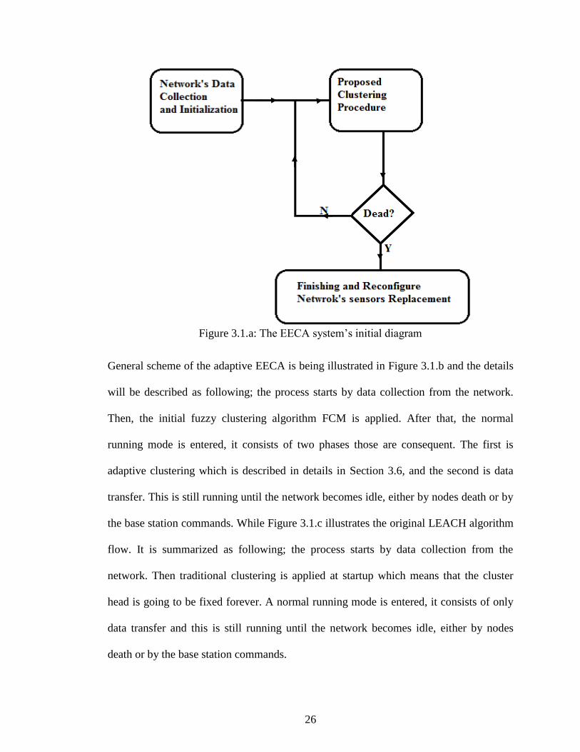
Figure 3.1.a shows the general mode of the Energy Efficient Clustering Algorithm
“EECA” adaptive software system. Starting by network data collection, it includes the
calculation, determining the energy of each sensor and the initial nodes clustering
(distributing on the cells) over the measurement space and initialization.
The initialization is plotting the location of each sensor in measurement space and
applying (FCM) traditional clustering algorithm to get the starting location of the head
of each cluster. That done after receiving the number of clusters that is needed to be used
for cells from the base station.
The next is to start the EECA clustering procedure, which is continue overall running
period of the network. During this mode, the network is re-clustered every transfer time
and re-localizes a new head of cluster and new distribution of nodes (sensors) in the cells
(clusters). When the nodes start to die, the base station should stop collecting data from
the network and generates the decision and command to replace the sensors.
26
Figure 3.1.a: The EECA system’s initial diagram
General scheme of the adaptive EECA is being illustrated in Figure 3.1.b and the details
will be described as following; the process starts by data collection from the network.
Then, the initial fuzzy clustering algorithm FCM is applied. After that, the normal
running mode is entered, it consists of two phases those are consequent. The first is
adaptive clustering which is described in details in Section 3.6, and the second is data
transfer. This is still running until the network becomes idle, either by nodes death or by
the base station commands. While Figure 3.1.c illustrates the original LEACH algorithm
flow. It is summarized as following; the process starts by data collection from the
network. Then traditional clustering is applied at startup which means that the cluster
head is going to be fixed forever. A normal running mode is entered, it consists of only
data transfer and this is still running until the network becomes idle, either by nodes
death or by the base station commands.

27
Figure 3.1.b: Basic Block Diagram of the EECA System
Figure 3.1.c: Basic Block Diagram of the Traditional LEACH Algorithm
28
3.2 Energy
The power consumption of any device can be represented in many ways. Actually, the
energy is being measured in “Joules” and has the “J” abbreviation. The power
consumption is measured in “Watts” and is abbreviated as “W”. Watt is the energy
consumed in one time unit. Usually, the system’s power is represented by the
manipulated variables – not direct variable – like voltage and current. The voltage is not
changes depending on the load, the manipulated variable of batteries become the current
and time.
Batteries in general are being rated as “Amp-hour” or “mAH” regards to milliamp hour.
Milliamphour means by theory that, i.e. if the battery is being rated as 50mAH, if the
load consumes 50mAmp, then, the battery can run this load for one hour. If the load
consumes 20mAH, then, the battery can be operated on this load for 2.5 hours. But from
practical view, this is not completely true, due to the chemical structure of the battery
[24].
In wireless sensors network, the battery is fixed and wouldn’t be replaced until the
sensor is replaced. The sensors are designated for a long time operation of its internal
battery. The life time of battery may extend to 5 or more years.
This thesis aims to optimize the energy consumption of the wireless sensors nodes by
optimizing the protocol of LEACH introducing a new terms and algorithms of nodes
clustering in order to make the network to be adapted to the work conditions.

29
3.3 Evaluation Metrics
The evaluation metrics is the measurements and criteria that are being used to evaluate
and test the wireless sensor networks quality and operation. It implies a high level
criteria and network aimed functionality in addition to long time running period. These
metrics will be met at optimal value to ensure the benefits of the wireless sensor
networks in comparison with other technologies [25].
The evaluation metrics includes a key variables that should be monitored and recode its
validity. Those variables describe the capabilities of the wireless sensor networks and
include
Cost.
Power dissipation.
Coverage.
The ease to use and deploy.
Life time.
Security.
Accuracy.
Effective sampling rate.
Response time.
Sometimes, those metrics are dependent to other, so, in order to increase one metric
variable, another variable should be changed. For example: in order to increase the life
time, the power dissipation should be minimized.

30
This work proposes the distance between the nodes to be measured by the Euclidean
distance. The strait line distance between two points is mathematically known as
“Euclidean distance” (or Eq.Dist). The points those subjected to calculate the Eq.Dist
may be placed with respect to two dimensional or three dimensional spaces, or even on a
dimension of line. Equation 3.1 is the mathematical representation of Eq.Dist in two
dimensional x-y coordinate plans. Here, the Eq.Dist will be calculated between two
points named p, q respectively [9].
( ) ( ) √( ) ( ) ( ) …(3.1)
3.4 Fuzzy Logic
To illustrate the concept of fuzzy logic, consider for example the tall of human. When it
should be decided that, one person is tall or short? In digital concepts and digital
decisions, if the person is taller than threshold value, then he will be tall, otherwise he
will be short. For example, if 175 cm considered being the threshold value of tall people,
the digital concepts consider the 175 cm tall person to be tall whereas, the 174 is being
considered to be short. Is that right? Definitely it is not [26].
The fuzzy logic introduces the concepts of fuzzy sets and fuzzy decision where the tall is
represented in waiting function that is so called Member Ship Function “MFS”. The
membership function is a mathematical representation curve that represents the weight
of the decision. Figure 3.2 shows the most commonly used membership functions [27].

31
Figure 3.2: Different Types of Commonly used Member Ship Functions [27]
For such weighted functions, the decision will be if the person’s tall being 200cm then
this person is tall in 1.0 percent while if his tall being 165cm, then it will be tall in 0.55
percent for example, while, the 155cm person is tall with 0.2 percent.
Also, fuzzy logic introduces multi decisions for the same variable. For example, the
person of 170cm tall would have the following decisions:
TALL with 0.7 percent.
MEDIUM with 0.95 percent.
SHORT with 0.15 percent.

32
This is being done by suing three membership functions for the same variable which is
“tall”. The first “MSF” is “TALL”, the second is “MEDIUM”, and the third is
“SHORT”.
Figure 3.3 shows a variable that is being represented by fuzzy membership functions.
The y-axis represents the weight value where the x-axis represents the measured or
estimated value of that variable. In such, there are six membership functions those are:
“Remote”, “Very High”, “Low”, ”High” “Moderate”, “Very Low”. That variable is
being built with a modified “Gaussian” membership function.
Figure 3.3: An example of a variable that represented in fuzzy form with six member ship
functions [27].
3.5 Clustering
Nodes classification in clusters (cells) is the core of the LEACH protocol and its
extensions (i.e. LEACH-M, LEACH-L). In general, grouping a set of points (nodes) into
cells or clusters is interested methodology in modern applications and researches,
especially, in networking and scalability of the networks.

33
The grouping a bulk of nodes into clusters is highly dependent on the deployment
specifications, system’s architecture, scheme of bootstrapping, cluster characteristics,
etc. The center of the cluster is commonly known as Head of Cluster “CH”. The head of
cluster is one of the cluster’s nodes. The number of nodes in one cluster is almost differs
from it in the other clusters. Where the head of cluster can form in some systems a
second tier of the network and thus, another hieratical level can be formed, or it may be
just the data to another point [28].
The clustering in theory has many advantages in addition to the network scalability
support. Also, it minimized the routing table’s size that stored at individual nodes, and
allows to safe the bandwidth of the communication because it limits the cluster
interactions scope to the head of clusters, the redundancy avoiding would result and
change among nodes is being enabled.
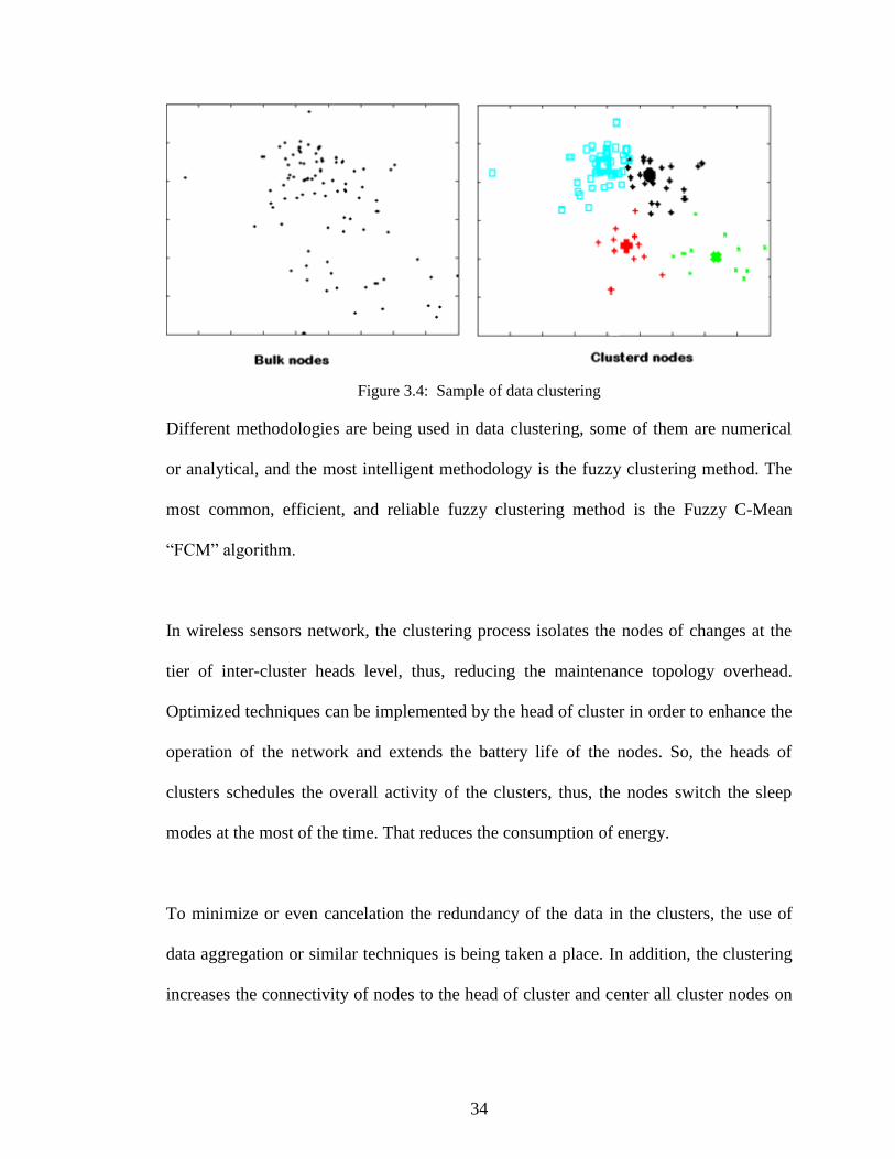
Figure 3.4 shows a sample of bulk data clustering in the left, and that is being clustered
in the right side. The Figure shows two dimensional distributed nodes, then, it classified
into four clusters. Each cluster is colored with unique color.
34
Figure 3.4: Sample of data clustering
Different methodologies are being used in data clustering, some of them are numerical
or analytical, and the most intelligent methodology is the fuzzy clustering method. The
most common, efficient, and reliable fuzzy clustering method is the Fuzzy C-Mean
“FCM” algorithm.
In wireless sensors network, the clustering process isolates the nodes of changes at the
tier of inter-cluster heads level, thus, reducing the maintenance topology overhead.
Optimized techniques can be implemented by the head of cluster in order to enhance the
operation of the network and extends the battery life of the nodes. So, the heads of
clusters schedules the overall activity of the clusters, thus, the nodes switch the sleep
modes at the most of the time. That reduces the consumption of energy.
To minimize or even cancelation the redundancy of the data in the clusters, the use of
data aggregation or similar techniques is being taken a place. In addition, the clustering
increases the connectivity of nodes to the head of cluster and center all cluster nodes on

35
the cluster head. This reduces the delay of measurement transfer and communicating to
the base station. It comprises the maximum network longevity.
3.6 The Proposed Clustering Algorithm
The EECA is an adaptive developed structural algorithm that locates the head of cluster
by cluster centroid localization of data set that consists of geometric distribution of
sensor-nodes in x-y plan or even capable to be used in 3-D space of sensing. EECA is
based on the original Fuzzy C-mean algorithm of clustering data in 2-D plan, and
improving it that by the use of “Potential” concept of the networks nodes and clusters.
When calculating the overall sensor-nodes potential to the centroid that is being obtained
from FCM, the nodes will be distributed into clusters easily by the mean of its potential
not Euclidean distance.
In the contributed EECA algorithm, once the potential of each node is calculated, the
head of cluster (CH) will be localized via the traditional FCM algorithm. The clustering
process will follow the last centroid (head of cluster) determination phase. This will be
determined and localized using the current suggested modification (addition) to the
fuzzy approach of clustering. The developed procedure in this thesis will generate
clusters that are equivalent in potential. Equation 3.2 expresses the contributed potential
mathematical form.
…. (3.2)

36
Where: P is the Potential.
Eq: is the Euclidian distance.
Er: is the total remaining energy in the sensors battery.
D is the transmission data cost function.
Tq is the energy slop of transmission data.
K is the battery self-leakage.
This equation calculates the potential of the node, and it represents a non-linear relation
between the Euclidean distance (see Equation 3.3 above), and the sensor’s current
working energy (which is the maximum initial energy minus the running cost energy), in
addition to the energy cost (assumption) of each data bit; the energy consumption is
known as (energy slope).
When the potential is taken into consideration, the specification of internal battery surely
has leakage. Its leakage is represented by the Equation 3.3 [9].
( ) ( ) √∑ ( ) ….. (3.3)
The above equation illustrates how to calculate the Eq.Dist between target point “q” and
destination pint “p”. Here the distance is “d”. The destination point may be the head of
cluster or normal node [9].

37
For communication purposes with the BS (Base Station), various or different frequency
levels and gaps may differ from area to area or from sensor to sensor. This thesis focuses
on clustering energy optimization, so, the frequency and communication power is being
expressed by the mean of slope of the energy for each sensor’s-node. This work
implements MATLAB procedures and functions to simulate the contributed EECA and
comparing it with the well-known LEACH algorithm and its extensions. The prolonging
of the overall time that the network can work in is clear from the result of the simulation.
The proposed methodology of the thesis consists of three phases. The bulk network of
sensors should be divided into clusters and that process is so called “Clustering”. The
thesis assumed to use the fuzzy logic approach of clustering by what is called C-mean.
The phase one distribute the sensor points into separate clusters, each cluster has its own
head. That clustering is potential-based as illustrated in this chapter above. Equation 3.2
is being used to calculate the contributed potential.
The data transfer (protocol data, measurement physical variables data, and status) will
proceed starting from each node in the cell or cluster to communicate with the base
station. This communication doesn’t pass directly, the node communicates with CH
(cluster head), and all heads will transfer data directly to/from the main unit (base
station). After each single transmission round, the sensor loses a part of its energy. The
power consumption is named above to be named as (slope of the energy).
Communicating was the second phase, while in the last phase, the cluster head will be
changed continuously with every communication round process. The contributed

38
adaptive EECA assumes the CH (head of cluster) to be changed in order to save it the
maximum power node. Equation 3.4 shows the mathematical expression that is being
used to calculate the commutative head of cluster. Once, a new cluster head is being
selected; all nodes will be re-clusters again. That will keep all clusters to be saved or got
similar energy levels.
( ∑( ) ( )) … (3.4)
The new heads of the clusters will be determined by their potential (pc), with respect to
the old potential of the heads of clusters (pco).
Those operational processes should continue running and re-selecting the clusters and
head of clusters. This proposed scheme will be active and running during all the time of
network run. The calculating of new suitable heads will be localized at every round.
Bellow the next Figure (3.5), displays a topology of clustered WSN in 2-D. In such
Figure, there are three types of nodes, the first those is bold and big which is the head of
clusters. The second has a single color, where those are node related to a cluster head
that has the same color. Whereas, the bi-colored points, is a sensor-nodes those has a
mid-potential between two clusters.
Those nodes can be categorized in each of the two clusters without a significant change
in the cluster itself. In the fact, these small changes could be used to balance the
potential of clusters. The points that are located potentially between two heads will be

39
named in this thesis as “In-Between Nodes”. Figure 3.5categories the network into four
cells.
Figure 3.5: Sample scheme of clustered WSN for the nodes in between two clusters- depending
on the potential of the each cluster.
This contributed algorithm, doesn’t generate exactly a cells those has typically the same
potential, but the difference of potential between them has a limit may reaches to zero or
near to zero, and thus, that difference will be neglected. The EECA aims to generate
such equi-potential cells. This contribution saves 3% or more for the total cells energy.
This result (3%) is gotten by simulating the network with and without the process of
managing the “In-Between Nodes”.
The LEACH algorithm extensions (either M or L) aim to make the life time of the nodes
to be maximum, but in both, once the first node is dead, a problem occurs. The problem
is that, the dead sensors will not be able to measure the physical data and cannot transfer
any data to the head of cluster node. So, it should be imagined that, one of the two
scenarios may happen once the first node is dead. The first scenario is that, the network
still working as it is, thus, one node cannot log the measured data. While the process

40
continues, more nodes will start dead and thus, a non-negligible data will be loosed, and
the network becomes un-useful. The second scenario is that, the network sensor nodes
are being replaced in the start time of nodes death, thus, a high cost will be achieved.
Then, the contributed EECA aims to minimize the period between the first and last node
death. This will keep the network running in balance measurements and data collection,
and also, it saves more power.
Many researchers performed experiments and researches to save network energy,
specially the energy between the first and final node death. This thesis, implements a
very effective and adaptive approach, that minimizes significantly the energy lose and
cost.
The best algorithm that saves the energy in interval of nodes death is LEACH-L before
testing the EECA approach. It increases the balancing in the nodes, thus, the use of low
power nodes converted to high power nodes. This contributed thesis increase the
efficiency to 90% rather than LEACH-L.
In this thesis, the key point in the developed EECA is making all nodes died in the same
time (that means the interval becomes near to zero) that why it is an efficient clustering
procedure for cells. The adaptation means that, the cluster head will not be fixed – even
it is still has large power in the cell -. It will be changed to keep on the balancing of the
cluster. Thus, the nodes distribution will be balanced with respect to its potential, and it
results the balance energy slope and power consumption of all nodes. The generated
clusters will be symmetrical along the overall running period.

41
Furthermore over that, the head of cluster should be kept as it is the larger potential node
over all running time. This requires re-clustering all of the data at each round. This
makes a benefit of decreasing the power consumption of the leave nodes where that is
considered to be head in the traditional LEACH procedure or its extensions. The wrong
cell center (Head of clusters) is almost leaks a big value of energy. On the other hand,
the contributed Energy Efficient Clustering Algorithm “EECA” contributes intelligent
solutions for that problem, and thus, saves an interesting value of the cell’s power.

42
Chapter 4
RESULTS
4.1 Performance Evaluation
This Thesis developed MATLAB program to experiment and simulate EECA algorithm
and getting the results. In such, two assumed areas are used for testing the protocol. The
wireless sensor networks are distributed in the two scope areas individually and both are
tested, and the parameters measured individually.
The “round” concept represents a complete transmission process over running of the
wireless sensors network.
The first scope is 300 by 300 m, where the second is 500 by 500 m. Initial conditions
and test conditions are illustrated in Section 4.2. The test will consider almost on the
energy optimization measurements with respect to a LEACH, LEACH-M, and LEACH-
L protocols. The result will be compared and discussed in Section 4.3.
Table-4.1 bellow illustrated the assumed parameters that have been implemented in
simulation for testing purpose. Those parameters are selected in order to make the
comparison between the EECA protocol and the other LEACH protocols more
meaningful. Thus, the new modifications, improvements, and optimization – especially
in energy – are clearer in the Figures.

43
The trends and Figures illustrated the energy scope and performance. The energy
consumption will be shown in Figures to show how the energy is being consumed. The
dead node trends show the node activity until it died. The overall nodes death displays
the performance of the network optimization.
The testing of EECA is done in two topological scenes; the first is over 500 by 500
meters, while the other comprises 300 by 300 meters.
Table 4.1: Simulation Parameters [9]
Parameter Test conditions 1 Test conditions2
Network validity scope “m” 300 by 300 500 by 500
No# of wireless sensors 900 2500
Energy at Starting 0.5 J 0.5 J
E (J)energy parameter 1 1
Transmission packet length
“bits”
4000 4000
E(DA) (Energy required for data
aggregation)
5 x 10⁻⁹
5 x 10⁻⁹
P(cluster-head section probability
used during cluster creation) 0.1 0.1
M (Multipath-Fading) 0.1 0.1
D (distance between transmitter
and receiver)
70 m 70 m
Transmission-Distance(m) 30 70

44
4.2Experimental Result
From the Figures bellow, it’s easily and clearly to see that, the contributed Energy
Efficient Clustering Algorithm “EECA” comprises the minimized power consumption
via time unit. So, the backup power of the sensors will be saved for longer time.
The cycle across the total running time of the network of 300X300 m results are
displayed in Figure 4.1. From the Figure, it’s clear that, the nodes using the EECA
algorithm are running for more number of cycles than the others and the death of the
nodes is very balanced in the contributed EECA algorithm. While in comparison to other
LEACH schemes, there is a larger interval. Again, that cause to save more power and
energy by prolong the nodes running time.
Figure 4.1: Nodes Death over 300 x 300 round in different protocols.

45
Whereas Figure 4.2 displays the nodes death scheme for an area of 500 by 500m. It can
be shown that EECA algorithm has two benefits: The system is running for more
number of rounds than using other LEACH protocols and the time death interval
between the first and last node is the shorter than others. So EECA system can minimize
the death nodes interval, reduce the power consumption, save more energy and prolong
the lifetime of the nodes.
Figure 4.2: Dead Nodes over a round of 500 x 500 in different protocols

46
The next two Figures show the received packet number in time interval of all LEACH
protocols in addition to the EECA protocol tested in 300x300m WSN space, and
500x500m WSN space respectively.
Figure4.3 displays the relation of the amount of sent packets during their life interval in
an area of 300 by 300m. It shows that EECA system can transmit more number of
packets than other LEACH protocols for a longer period of time and can clarify the very
helpful linearity implementation that ensures the progress of data packet communicating
plus the increasing in number of transmitted packets.
Figure 4.3: Received packets over round of 300 x 300 in different protocols

47
While Figure 4.4 displays the transmitted packets number in time interval for an area of
500 by 500m. It can be noticed that the EECA system increases the amount of
transmitted packets, keep on communicating for more number of cycles and minimize
the time death interval between the whole nodes which leads to improve the
performance of the system.
Figure 4.4: Received packets over round of 500 x 500 in different protocols
The next two Figures show the direct relation between the power consumption with the
number of cycles for an area of 300 by 300m and 500 by 500 m respectively.
48
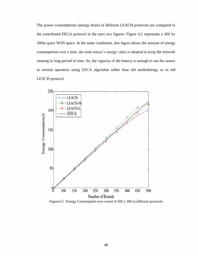
The power consumptions (energy drain) of different LEACH protocols are compared to
the contributed EECA protocol in the next two figures. Figure 4.5 represents a 300 by
300m space WSN space. In the same conditions, this figure shows the amount of energy
consumptions over a time, the total sensor’s energy value is adopted to keep the network
running in long period of time. So, the capacity of the battery is enough to run the sensor
in normal operation using EECA algorithm rather than old methodology as in old
LEACH protocol.
Figure4.5: Energy Consumption over round of 300 x 300 in different protocols

49
The power consumption of the contributed EECA protocol is compared to the old
LEACH protocol in the next figures. Figure 4.6 is representing a 500 by 500m WSN
space. In the same conditions, this figure shows the amount of energy consumptions
over a time, EECA algorithm adopted the total sensor’s energy value to keep the
network running in long period of time. So, the capacity of the battery is enough to run
the sensors in normal operation rather than old methodology.
Figure 4.6: Energy Consumption over round of 500 x 500 in different protocols

50
Table 4.2 shows the energy optimization efficiency that is achieved using the EECA
algorithm of variable clustering of the wireless sensor networks comparison with the
different algorithms that is used.
Table 4.2: Energy optimization of different clustering algorithms
Algorithm
Energy Optimization Percent
EECA 93%
LEACH-M 80%
LEACH-L 65%

51
Chapter 5
CONCLUSION
This research concerns to implement a new methodology for wireless sensors adaptive
clustering in order to optimize energy and power consumption in the network. Many
researches in past and current information systems world are concerning in the energy
optimization. The optimization of wireless network energy researches either concerns on
hardware modification and optimization or either software management.
The past researches on clustering of wireless sensor networks got a result of saving an
interesting amount of energy and sensor’s life.
This research added a value of saving more energy and power, and building adaptive
algorithm. This algorithm as shown in chapter four, was been tested on different scopes
of wireless sensors networks in different conditions. From that point the following
conclusions have been got:
The energy of wireless sensor networks is important issue and needs more hardware
and software solutions to get good optimization methods.
Energy optimization can significantly be done by a suitable clustering algorithm.

52
This research is a novel clustering algorithm for improving the conservation of
energy in WSN’s.
Hence, the asymmetry of clusters (cells), the nodes will consume asymmetrical
power, due to the asymmetrical structure, design, and pocket data transfer. While, it
can be managed to balance the cluster’s load by introducing a specific variable or
concept that can express the overall load of the cluster and also node. Whereas this
variable or concept should be mathematically and physically meaningful for all
conditions and variables that affect the sensors battery and cluster communication
transfer. This variable or concept is so called in this thesis “POTENTIAL”.
This thesis, introduces the “POTENTIAL” concept of the wireless sensors network.
The potential of the node represents the availability of that node (sensor) to transfer
data and for how long a time.
The POTENTIAL of the cell is the availability of the cluster of sensors to measure
and send data for a how long time.
In thesis, the symmetry of all clusters (Cells) enables all clusters to work in the same
time long. Thus, all clusters will start to die at the same time. This ensures that, no
cluster work and other die.
Also, the symmetry inside the cluster, make to whole network nodes work in the
progress together for a time long, and the all nodes will start in death in the same
moment. This ensures a time interval for nodes death to be approaches zero.
53
The symmetry of the clusters and nodes can be achieved in different methodologies.
This paper use three methodologies and techniques to perform this approach. The
first one is to re-cluster all networks continuously after each transfer process.
Although, this will increase up the computational power, but this rise is always
negligible with comparison of optimization. The second technique is to make the
head of clusters to be variable, and all heads of clusters are being changed
continuously over the time after each data transfer process seemingly.
While, the third technique is to deal with specific sensor nodes, whose represents
sensors located in between two – or more – clusters. Those sensors can be added in
clustering process to any one of the clusters those the nodes located near to it without
any big change in cell load. The “in between” nodes is a good concept to handle. The
calibration of cluster balance can be done by controlling those nodes in order to fine
tune the POTENTIAL of the clusters. The small change of cluster’s potential can be
tuned using those nodes interestingly.
Fuzzy logic clustering is an intelligent method to distribute the nodes over the cells
or clusters, but its result is always generated Not-Equal sizes clusters and also, Not-
Equal Potentials.
This thesis introduced and implemented a new modification on the fuzzy C-mean
clustering algorithm. This modification uses the POTENTIAL to distribute the nodes
over the cells (clusters). The fuzzy C-mean clustering is used to determine the initial
nodes those can be represented as “head of clusters” and the modification of the

54
algorithm is to retest each node and add it to the appropriate cluster by
POTENTIAL.
The fact that, if we got symmetrical clusters by POTENTIAL over the time of data
transfer, then all nodes and clusters will start to die and die in the same time, leads to
implement the variable clustering algorithm. This clustering includes re-locating the
head of cluster after each transfer of data process, and then re-clustering all data.
5.1 Suggestions for Future Work
Many researches related to wireless sensor networks energy optimization are being
introduced in this time. The research that can achieve a good score and add an important
contribution is the research that solves the important problematic issues. Those include
energy optimization and power dispatch, data transfer, security, hardware reliability, and
management.
This research is concerning in software for energy optimization, it is a first stage of
performing energy and data saving across a total network running period or life. That is
including managing the measurements, data logging, transfer, energy optimization, and
replacement.
The future work that is closely related to this thesis is concerns in two axes. Those axes
should be implemented and developed to complete the full system optimization. Those
are:
1. Adapting management protocol that manages both, the data transfer and clustering
algorithm. This protocol is the main control protocol of base station.

55
2. Implementing measurement, data logging, and transfer protocol that comprises the
energy and performance saving.
Ongoing, the PhD of mine will be a completion work on this side of researches. The
problems that should be solved and dealing with in PhD thesis are the following:
Handling the control and management protocol of the EECA directly from the
base station, while it was automatic in this thesis.
Dealing with the In-Between nodes automatically.
Handling the far nodes, where those were excluded from this research.
Dealing with tracking applications and real-time physical data measurements and
logging.
Contributing an intelligent technique for activation / deactivation of nodes
depending on area of interest for measurement.

56
REFERENCES
[1]Seema Bandyopadhyay and Edward J., Coyle, “An Energy Efficient Hierarchical
Clustering Algorithm for Wireless Sensor Networks”. IEEE Conference INFOCOM
2003, pp. 189-200.
[2] Heinzelman W., Chandrakasan A., and Balakrishnan H., “Energy-Efficient
Communication Protocol for Wireless Micro sensor Networks”, In Proceedings of the
Hawaii Conference on System Sciences, Vol. 2, No. 8, 2000, pp. 584-598.
[3] Cerpa A., “Habitat Monitoring Application Driver for Wireless Communications
Technology”, In proceeding of ACM SIGCOMM, 2001, pp. 20-41.
[4] Philipp S., and Roger W., “Gradient Clock Synchronization in Wireless Sensor
Networks”. In 8th ACM/IEEE International Conference on Information Processing in
Sensor Networks (IPSN), San Francisco, USA, April 2009, pp. 421-442.
[5] Geoffrey W., Konrad L., Matt W., Omar M., Jeff J., Mario R., and Jonathan L..
“Deploying a wireless sensor network on an active volcano”, IEEE Internet Computing,
2006, pp. 18–25.
[6] Doherty L., Pister J. and Ghaoui E., “Convex position estimation in wireless sensor
networks” IEEE Computer Society Press, Vol. 38, No. 4, 2001, pp.1655-1663.

57
[7] Mainwaring A., “Wireless Sensor Networks for Habitat Monitoring”, In proceeding
of (WSNA'02), 2002, pp. 88-97.
[8] Shah R., Roy S., Jain S., and Brunette W., “Modeling three tier architecture for
sparse sensor networks”, In Proceedings of the First IEEE Workshop on Sensor Network
Protocols and Applications (SNPA), 2003, pp. 30-41.
[9] Fengjun S., Yang L., “An Energy-Balanced Clustering Routing Algorithm for
Wireless Sensor Network” Scientific Research Journal, Vol.2, No. 10, 2010, pp. 777-
783.
[10] Tony R. K.,” Lesson In Electronic Circuits”, Vol 2-AC, 6th Edition, (Book) 2007,
http://www.mdp.eng.cam.ac.uk/web/library/enginfo/textbooks_dvd_only/lessons_pdf/A
C.pdf.
[11] Yarvis D., “Real-World Experiences with an Interactive Ad Hoc Sensor Network”,
In International Conference on Parallel Processing Workshops, 2002, pp.143-151.
[12] Ye W., Heidemenn J., and Estrin D., “An Energy-Efficient MAC Protocol for
Wireless Sensor Networks”, http://www.isi.edu/ilense/macss/, 2001, Technical Report.
[13] Wang C., Zhang K. and Wang C., “A secure routing protocol for cluster-based
wireless sensor networks using group key management”, In 4th IEEE International

58
conference on Wireless Communications, Networking and Mobile Computing
(WiCOM08), 2009, pp. 1-5.
[14] Fan N. and Song L., “Improvement on LEACH Protocol of Wireless Sensor
Networks” Proceedings of 2007 International Conference on Sensor Technologies and
Applications, Valencia, 2007, pp. 260-264.
[15] Pottie G. and Kaiser W., “Wireless Integrated Network Sensors (WINS): Principles
and Approach” In proceeding of Communications of the ACM, Vol.43, No. 5, 2000,
pp.51-58.
[16] Mclurkin J., “Algorithms for distributed sensor networks” Master’s Thesis for
Electrical Engineering at the University of California, Berkeley, 1999, http://www.
cs.rice.edu/~jm23/publications/McLurkin-MS-UCB-1999.pdf, Technical report.
[17] Geng Y., Hong-bing C. and Su-jun H., “A novel hierarchical routing protocol
algorithm for wireless sensor networks” Science Direct, Vol. 15, 2008, pp. 75-81.
[18] Hu G., Wu D. and Ni G., “Research and improve on secure routing protocols in
wireless sensor networks” In 4th IEEE International Conference on Circuits and Systems
for Communications, 2008, pp. 853-856, Technical report.

59
[19] Zhu S., Setia S., Jajodia S., “LEAP: Efcient security mechanisms for large scale
distributed sensor networks”, 10thACM Conference on Computer and Communication
Security, ACM Press, New York, 2003, pp. 62-72.
[20] Whitehouse K., “The design of calamari: an ad-hoc localization system for sensor
networks”, Master Thesis, University of California, http://www.cs.virginia.edu/~white
house/research/localization/whitehouse02calamari.pdf, 2003, Technical report.
[21] Shibo W., Selc K., “Power-aware single and multipath geographic routing in sensor
networks”, Uk-Canda, Ad Hoc Networks Journal 5, 2007, pp. 974–997
[22] Perrig A., “SPINS: Security protocols for sensor networks” Proceedings of
MOBICOM, Wireless Networks 8, 2002, pp. 521-534.
[23] XinYn, “Distributed cache updating for the dynamic source routing protocol”, IEEE
Transactions on Mobile Computing, VOL. 5, NO. 6, JUNE 2006, pp. 609-621.
[24]Cao Q., He T. and AbdelZaher F., “Unified Connectionless Multicast for Energy
Efficient Content Distribution in Sensor Networks”, IEEE Transactions on Parallel and
Distributed Systems, Vol. 18, No. 2, 2007, pp. 240-250.
[25] Karlof C. and Wagner D., “Secure routing in sensor networks: attacks and counter
Measures” Ad Hoc Networks Journal, Vol. 1, May 2003, pp. 293-315.

60
[26] Stephen L. C., “Fuzzy model identification based on cluster estimation”, Rockwell
science Center Thousand Oaks, California 91360, http://chius.homestead.com/files/
FuzzyModelID.pdf, June 1994, Technical report.
[27] Isazadeh A. and Ghorbani M., “Fuzzy c-means and its generalization by Lp-norm
space”, WSEAS Transaction on Mathematics, Vol. 2, 2003, pp. 168-170.
[28]Georgios S., Ibrahim M., and Azer B., “A stable election protocol for clustered
heterogeneous wireless sensor networks”,http://dcommon.bu.edu/xmlui/bitstream/handle
/2144/1548/2004-022-sep.pdf?sequence=1, 2004, Technical report.
[29] Pister J., Kahn M., and Boser E., “Smart Dust: Wireless Networks of Millimeter-
Scale Sensor Nodes”, Electronics Research Laboratory Research Summary,
http://robotics.eecs.berkeley.edu/~pister/SmartDust/, 1999, Technical report.
[30] Stephanie Lindsey, Cauligi Raghavendra, “Power-Efficient Gathering in Sensor
Information Systems”, In proceeding of (PEGASIS), Vol. 3, 2000, pp. 1125-1130.
[31] Jamal N. Al-karaki and Ahmed E. Kamal., “Routing techniques in wireless sensor
networks: A survey”, IEEE Wireless Communications, Vol. 1, 2004, pp. 449-458.
61
[32] Philipp S., and Roger W., “Gradient Clock Synchronization in Wireless Sensor
Networks”. In 8th ACM/IEEE International Conference on Information Processing in
Sensor Networks (IPSN), San Francisco, USA, April 2009, pp. 37-48.
[33] Oliveira B., Habib E., Wong C., Ferreira C., Vilaa A., and Loureiro A., “Security of
cluster-based communication protocols for wireless sensor networks”, In 4th IEEE
International Conference on Networking (ICN05), volume Lecture Notes in Computer
Science, Washington, DC, USA, 2005, pp. 449-458.
[34] Gowda K.C., DidayE., “Symbolic clustering using a new similarity measure”, IEEE
Trans. System Man Cybernet, Vol. 22, 1992, pp. 368–378
[35] Hill J., “System architecture directions for networked sensors”, In proceeding of
ASPLOS, Vol. 28, No. 5, 2000, pp. 93-104.
[36] Roundy S., Wright P., and Rabaey J., “A Study of Low Level Vibrations as a Power
Source for Wireless Sensor Nodes”, IEEE Communications Journal 2002, pp. 1131-
1144.
[37] Scott M.D., “An Ultra-Low Power ADC for Distributed Sensor Networks” Master
of Science Thesis, UC Berkeley, 2002, pp. 3-13.

62
[38] Zhang H., Chen J. and Hu J., “An leniency security model of routing protocol in
wireless sensor networks” In Second Asia International Conference on Modeling and
Simulation, Washington, DC, USA, 2008, pp. 59-64.
[39] Vilaa M. A., Wong H. C., Bern M., Dahab R., L., Ferreira A. and Loureiro A. F.,
“Secleach-on the security of clustered sensor networks”, Vol.87, No.2, December 2007,
pp.2882-2895.
[40] Hill J., “System Architecture for Wireless Sensor Networks”, Master’s Thesis,
University of California Berkeley, 2000, Technical report.
[41] Bern M., Dahab R., Oliveira B., Wong C. and Loureiro F., “Secleach - a random
key distribution solution for securing clustered sensor networks”, In Fifth IEEE
International Symposium on Network Computing and Applications, Washington, DC,
USA, 2006, pp.145-154.

63
APPENDIX

64
Simulation Code
Function drawResults
figure(1); title('500x500 round node death')
loadEECARec.mat
hold on
plot(Rmea1(1,:),Rmea1(2,:),'g-','LineWidth', 2.1)
plot(RLa1(1,:),RLa1(2,:),'r-','LineWidth', 2.3)
plot(RLLa1(1,:),RLLa1(2,:),'b-','LineWidth', 2.2)
plot(RLMa1(1,:),RLMa1(2,:),'k-','LineWidth', 2.4)
hold off
clear;clc
loadLchRec.mat
figure(2); title('300x300 round node death')
hold on
plot(Rmeb2(1,:),Rmeb2(2,:),'g-','LineWidth', 2.1)
plot(RLb2(1,:),RLb2(2,:),'r-','LineWidth', 2.3)
plot(RLLb2(1,:),RLLb2(2,:),'b-','LineWidth', 2.2)
plot(RLMb2(1,:),RLMb2(2,:),'k-','LineWidth', 2.4)
hold off
clear;clc
figure(3); title('energy consuption')
hold on

65
loadLcLRec.mat
plot(Rmec2(1,:),Rmec2(2,:),'g-','LineWidth', 2.1)
plot(RLc2(1,:),RLc2(2,:),'r-','LineWidth', 2.3)
plot(RLLc2(1,:),RLLc2(2,:),'b-','LineWidth', 2.2)
plot(RLMc2(1,:),RLMc2(2,:),'k-','LineWidth', 2.4)
hold off
clear;clc
figure(4); title('round numb paket number')
loadLcMRec.mat
hold on
plot(Rmed1(1,:),Rmed1(2,:),'g-','LineWidth', 2.1)
plot(RLd1(1,:),RLd1(2,:),'r-','LineWidth', 2.3)
plot(RLLd1(1,:),RLLd1(2,:),'b-','LineWidth', 2.2)
plot(RLMd1(1,:),RLMd1(2,:),'k-','LineWidth', 2.4)
hold off
clear;clc
%==========================================================

66
functionfiras(n)
% set of points arrangement and plotting
loaddatasample.mat
fcmdata = scho;
fcmdata = abs(randn(40,2))*10;
fcmdata(:,3)=100; %starting battery energy of each sensor's node -
potential 1
fcmdata(:,4)=rand(40,1); %energy consumption slope - potential 2
% potential 3 = Euclidean distance value
[r0 c0]=size(fcmdata);
figure;plot(fcmdata(:,1),fcmdata(:,2),'.k')
title('Data Set')
%==========================================================
%getting cluster centers from fuzzy logic clustering
[allcenters, U, obj_fcn] = fcm(fcmdata, n); %fuzzy c-mean
clustering
maxU = max(U);
plotstyle=['bo'; 'gx'; 'r+'; 'k*'; 'cs'; 'yv']; %array of plot style and colors
pause
figure(2)
for k=1:n
hold on
%==========================================================
plot(allcenters(k,1),allcenters(k,2),plotstyle(mod(k,6)+1,:),'markersize',14,'LineWidth',6)
%plotting the colored centers of clusters
end
%==========================================================

67
%clustering the overall points using potentials
%figure(4) %
%create new figure; and hold the figure
fortyt=1:100
pause
if(tyt>1)
figure(4)
close(4);hold on
figure(4)
else
pause
figure(3)
end
%%&&&&&&&&&&&&&&&&&&&&&&&&&&&&&&&&&&&&&&&&&&
n2=1;
[a,b]=size(fcmdata);
tempfull=zeros(a,b);
ind1=1;
fcmcopy = zeros(a,b+1);
fcmi=0;
fcmdata(:,3)=fcmdata(:,3)-fcmdata(:,4);
for k=1:n
center{k}=allcenters(k,:);
eq{k}=dist(center{k},fcmdata')';
tr1=eq{k};
potential = (tr1)+ (1./fcmdata(:,3)).*(1./fcmdata(:,4));
conx(:,1)=potential;
conx(:,2:5)=fcmdata(:,1:4);
for i=1:r0

68
for j=1:r0-1
if(conx(j,1)>conx(j+1,1))
sorx=conx(j,:);
conx(j,:) = conx(j+1,:);
conx(j+1,:) = sorx;
end
end
end
conx;
count=ceil(r0/n)
clust{k}=conx(1:count,:);
clustx =conx(1:count,:);
context(:,1:3)=conx(1:count,2:4)
allclusters(:,:,k) = clustx;
clusmin=min(context(:,3));
[u0 p0]=size(context);
for w=1:u0
if(context(w,3)==clusmin)
break;
end
end
newcenters(k,:)=context(w,1:2);
if(tyt>1)
for i=1:count
text(context(i,1), context(i,2), num2str(context(i,3)));
end
end

69
end
savecomdata.mat tr1
%=============================================================
hold on
for i=1:k
plot(allclusters(:,2,i),allclusters(:,3,i),plotstyle(mod(i,6)+1,:))
%plotting the points in cluster color
end
for k=1:n
centerx=center{k};
plot(centerx(1,1),centerx(1,2),plotstyle(mod(k,6)+1,:),'markersize',14,'LineWidth',6)
%plotting the colored centers of clusters
end
centerx=newcenters
%%&&&&&&&&&&&&&&&&&&&&&&&&&&&&&&&&&&&&&&&&&
end
Related Documents