An Empirical Test of the Relative Validity of Expert and Lay Judgments of Risk

Risk Analysis, Vol. 22, No. 6, 2002

An Empirical Test of the Relative Validity of Expertand Lay Judgments of Risk

George Wright,1∗ Fergus Bolger,2 and Gene Rowe3

This article investigates how accurately experts (underwriters) and lay persons (university stu-dents) judge the risks posed by life-threatening events. Only one prior study (Slovic, Fischhoff,& Lichtenstein, 1985) has previously investigated the veracity of expert versus lay judgmentsof the magnitude of risk. In that study, a heterogeneous grouping of 15 experts was found tojudge, using marginal estimations, a variety of risks as closer to the true annual frequencies ofdeath than convenience samples of the lay population. In this study, we use a larger, homoge-nous sample of experts performing an ecologically valid task. We also ask our respondents toassess frequencies and relative frequencies directly, rather than ask for a “risk” estimate—aresponse mode subject to possible qualitative attributions—as was done in the Slovic et al.study. Although we find that the experts outperformed lay persons on a number of measures,the differences are small, and both groups showed similar global biases in terms of: (1) over-estimating the likelihood of dying from a condition (marginal probability) and of dying froma condition given that it happens to you (conditional probability), and (2) underestimatingthe ratios of marginal and conditional likelihoods between pairs of potentially lethal events.In spite of these scaling problems, both groups showed quite good performance in orderingthe lethal events in terms of marginal and conditional likelihoods. We discuss the nature ofexpertise using a framework developed by Bolger and Wright (1994), and consider whetherthe commonsense assumption of the superiority of expert risk assessors in making magnitudejudgments of risk is, in fact, sensible.

1. INTRODUCTION

In a pioneering paper, Lichtenstein, Slovic,Fischhoff, Layman, and Combs (1978) investigatedhow well people (students and convenience samplesfrom the lay population) could estimate the frequency

1 Graduate School of Business, University of Strathclyde, 199Cathedral Street, Glasgow G4 0QU, UK.

2 Department of Management, Bilkent University, 06533 Bilkent,Ankara, Turkey.

3 Institute of Food Research, Norwich Research Park, Colney, Nor-wich NR4 7UA, UK.

∗Address correspondence to George Wright, Graduate Schoolof Business, University of Strathclyde, 199 Cathedral Street,Glasgow G4 0QU, UK.

of the lethal events that they may encounter in life.These investigators argued that “Citizens must as-sess risks accurately in order to mobilize society’s re-sources effectively for reducing hazards . . . . officialrecognition of the importance of valid risk assess-ments is found in the ‘vital statistics’ that are care-fully tabulated . . . there is, however, no guarantee thatthese statistics are reflected in the public’s intuitivejudgments” (1978:551). In their study, Lichtensteinet al. (1978) found that although their subjects exhib-ited some competence in judging such frequencies—frequency estimates increased with increases in truefrequency—the overall accuracy of both (1) pairedcomparisons of the relative frequency of lethalevents and (2) direct estimates of individual events’

1107 0272-4332/02/1200-1107$22.00/1 C© 2002 Society for Risk Analysis

1108 Wright, Bolger, and Rowe

frequencies were poor.4 In a comment on theLichtenstein et al. study, Shanteau (1978) argued thatif respondents had had more experience with thelethal events, the validity of the required estimatesmay have shown improvement. He concluded that“It might also be of some value to investigate judg-ment of lethal events using subjects who have directknowledge and exposure to such events (such as lifeinsurance analysts)” (1978:581).

Since the 1978 paper, research on risk judgmentshas led to the generally accepted conclusion thatexpert judgments are, indeed, more veridical thanthose of the general public (e.g., Slovic, 1987, 1999).One basis for this argument is the work by Slovic,Fischhoff, and Lichtenstein (1985). In this study, theauthors utilized samples of the U.S. League of WomenVoters, university students, members of the U.S.Active Club (an organization of business and profes-sional people devoted to community services activi-ties), and a group of “experts” (comprising 15 peoplewho were described as professional risk assessors, in-cluding a geographer, an environmental policy ana-lyst, an economist, a lawyer, a biologist, and a govern-ment regulator of hazardous materials). Perceptionsof risk were measured by asking participants to orderthe 30 hazards from least to most risky (in terms of the“risk of dying (across US Society as a whole) as a con-sequence of this activity or technology” (1985:116)).Participants were told to assign a numerical value of10 to the least risky item and to make other ratings rel-ative to this value. Since these instructions called fora risk assessment, rather than a frequency or relativefrequency estimate (cf. Lichtenstein et al., 1978), theavenue was open—for both experts and nonexperts—for qualitative risk attributes, such as the voluntari-ness or controllability of the risk, to enter into theseglobal risk judgments.

Slovic, Fischhoff, and Lichtenstein (1985) con-cluded that the judgment of their experts differedsubstantially from nonexpert judgment primarily be-cause the experts employed a much greater range ofvalues to discriminate among the various hazards thatthey were asked to assess, which included motor vehi-cles, smoking, alcoholic beverages, hand guns, surgery,x-rays, and nuclear power. Additionally, Slovic,

4 However, these authors did not provide a standard of evaluationthat allowed the implications of this finding for subsequent deci-sion making to be determined. For example, would an individual’spersonal decisions about exposure to particular hazardous eventsbe sensitive to low accuracy in that individual’s assessment of theirfrequency?

Fischhoff, and Lichtenstein (1985) concluded thattheir obtained expert-lay differences were “becausemost experts equate risk with something akin to yearlyfatalities, whereas lay people do not” (1985:95). Thisconclusion is founded on the fact that the obtainedcorrelations between perceived risk and the annualfrequencies of death were 0.62, 0.50, and 0.56 for theLeague of Women Voters, students, and Active Clubsamples, respectively. The correlation of 0.92 obtainedwithin the expert sample is significantly higher thanthose obtained within each of the three lay samples.However, Slovic, Fischhoff, and Lichtenstein (1985)also found that both the lay and expert groupingsviewed the hazards similarly on qualitative character-istics such as voluntariness of risk, control over risk,and severity of consequences—when asked directlyto do so (see Rowe & Wright, 2001, for a full discus-sion). It would seem that, when asked for a “risk” esti-mate, Slovic et al.’s experts viewed this as a magnitudeestimation task rather than a qualitative evaluationtask. Additionally, an artificial ceiling may have beenplaced on the evaluation of the veracity of magnitudeestimates of risk made by the lay samples, if mem-bers of the lay groupings were more likely to view thetask of making a “risk” estimate as one of qualitativeevaluation.

Since Slovic, Fischhoff, and Lichtenstein’s (1985)study of expert-lay differences in risk judgment, sev-eral other papers have taken a similar theme. Thesehave used expert samples of toxicologists (Kraus,Malmfors, & Slovic, 1992; Slovic, et al., 1995), com-puter scientists (Gutteling & Kuttschreuter, 1999), nu-clear scientists (Flynn, Slovic, & Mertz, 1993), aquaticscientists (McDaniels et al., 1997), loss preventionmanagers in oil and gas production (Wright, Pearman,& Yardley, 2000), and scientists in general (Barke &Jenkins-Smith, 1993). These studies concluded thatthere are substantial differences in the way that ex-perts and samples of the lay population judge risk.Generally, experts perceive the risks as less thanthe lay public both across the wide variety of ques-tions asked and across the variety of substantive do-mains. The two exceptions are the studies by Wright,Pearman, and Yardley (2000)—where experts andmembers of the lay public shared similarities in riskperception of hazardous events in oil and gas produc-tion in the North Sea—and Mumpower, Livingston,and Lee (1987)—where the rating of the political risk-iness of countries by undergraduate students closelyparalleled the ratings of professional analysts. Boththese sets of results contrast sharply with results of

Relative Validity of Expert and Lay Risk Judgments 1109

Slovic, Fischhoff, and Lichtenstein (1985), describedearlier, where the experts saw 26 out of 30 activities/technologies as more risky than each of the three laygroupings. However, in all studies except for the latterstudy, the relative validity of expert versus layrisk assessments (in terms of the veracity of fre-quency estimates) has not been measured—hence, thecommonly accepted view about expert-lay differencesin risk judgments rests on the results of a single studythat used just 15 experts and that compared theirjudgments of “risk” with those of groups of lay per-sons on a task where the validity standard (mortalityrates) was not made salient to the lay group. Further,it would seem highly unlikely that the experts whotook part in the Slovic et al. study (e.g., a geographer,lawyer, and economist) could have had substantiveexpert knowledge in all of the variety of hazards thatwere utilized (including mountain climbing, nuclearpower, and spray cans), which begs the question: Werethey truly expert? This might also, in part, explain whythe results from this expert sample were inconsistentwith the results from expert samples in the other stud-ies. In a review of these studies, Rowe and Wright(2001) concluded that, contrary to received wisdom,there is little empirical evidence for the propositionthat experts are more veridical in their risk assess-ments than members of the public.

More widely, Bolger and Wright (1994) and Roweand Wright (2001) have argued that in many real-world tasks, apparent expertise (as indicated by, forexample, status) may have little relationship to anyreal judgmental skill at the task in question. In Bolgerand Wright’s review of studies of expert judgmentalperformance, they found that only six had showed“good” performance by experts, while nine had shownpoor performance and the remaining five showedequivocal performance. Bolger and Wright analyzedand then interpreted this pattern of performance interms of the “ecological validity” and “learnability”of the tasks that were posed to the experts. By “eco-logical validity” is meant the degree to which the ex-perts were required to make judgments inside thedomain of their professional experience and/or ex-press their judgments in familiar metrics. By “learn-ability” is meant the degree to which it is possiblefor good judgment to be learned in the task domain.That is, if objective data and models and/or reliableand usable feedback is unavailable, then it may notbe possible for a judge in that domain to improvehis or her performance significantly with experience(see, e.g., Einhorn, 1980; Keren, 1987). In such cases,

Bolger and Wright argued, the performance ofnovices and “experts” is likely to be equivalent.Bolger and Wright concluded that expert perfor-mance will be largely a function of the interactionbetween the dimensions of ecological validity andlearnability—if both are high then good performancewill be manifest, but if one or both are low thenperformance will be poor. For example, as pointedout by Murphy and Brown (1985), weather fore-casters in the United States and other countries areroutinely required to give confidence estimates at-tached to their forecasts. Such forecasts, say for thenext day’s weather, are succeeded by timely, uncon-founded feedback since very few interventions byman can confound the prediction/outcome relation-ship. It follows that experimental studies of weatherforecasters’ confidence in their weather predictionswill tend to be ecologically valid and that experimen-tal tasks will, most likely, use potential weather eventswhere the participating forecasters have experiencedprior conditions of learnability. Indeed, weather fore-casters do show good judgment (see Murphy andBrown, 1985, for a review).

From the perspective of Bolger and Wright’s anal-ysis, it is by no means certain that expert risk assessorswill be better at judging the veridical risks of hazardsthan lay persons, and the limited empirical evidencecannot be considered compelling (Rowe & Wright,2001). This has important implications for the com-munication of judgments of risk. As Rowe and Wright(2001) have argued, in hazard evaluations where thehazardous events happen rarely, if at all, then learn-ability will be low and the veridicality of judgmentsof the magnitude of risks by experts will be suspect.For example, consider the validity of expert predictivejudgments about the likelihood magnitude of humaninfection by “mad cow disease” resulting from eatingbeef from herds infected with Bovine Spongiform En-cephalopathy in the early 1990s and the subsequent,poorly predicted, mortality rates (Maxwell, 1999).In this instance, UK politicians used expert predic-tions to inappropriately reassure a frightened generalpublic.

The present study considers the issue of expert-lay differences in frequency, and relative frequency,judgments of lethal events using a sample of profes-sional risk assessors. It extends and develops the studyof Lichtenstein et al. (1978) and follows up the sugges-tion in Shanteau’s (1978) commentary on that paper.We utilize a sample of life underwriters, of varying de-grees of experience, and a task requiring assessment

1110 Wright, Bolger, and Rowe

of a varied set of potentially lethal events. In thenext two sections, we attempt to demonstrate thatthe expert-task relationship in this study has “eco-logical validity,” and hence, that inadequacies in ex-pert performance (if found) may reasonably be at-tributed to (lack of) expert performance and not topoor task design. First, we describe the nature ofthe experts used in this study and the tasks theyperform professionally and, second, we detail thenature of the judgments that we elicited from oursubjects.

2. THE NATURE OF OUR EXPERTS

The details of the underwriting process that tookplace at the insurance company from which under-writers were recruited in the present study are de-scribed in Bolger, Wright, Rowe, Gammack, andWood (1989). Essentially, financial advisors wouldsend applications for life insurance to local branchesof the company. If the applications were straightfor-ward (i.e., applicants were of an appropriate age, thesum to be insured was within reasonable limits, and nounusual circumstances were described on the form),then the branch would forward these to the new busi-ness department (NBD) to issue the policy. The deci-sions by the clerical staff at the branches were made onthe basis of a manual provided by the head office thatoutlined the factors that made a proposal acceptableor unacceptable. If the application was not straight-forward, the application would be forwarded to theunderwriters at the NBD for them to make the de-cision. The underwriters might then issue a policy, orreject the application or, often, send for additional in-formation, either medical information from a doctor,or personal information from the applicant (whichmight, for example, relate to a person’s hobbies orintended travel itineraries). See Rowe and Wright(1993) for a discussion of the life-underwriting taskand the extent to which underwriting judgment canbe modeled in automated expert systems.

At the time of Bolger et al.’s paper (1989), approx-imately 60% of proposals were accepted at branchlevel, and 40% were sent to the NBD underwrit-ers for assessment. The underwriters sought medi-cal evidence on approximately 20% of the cases theyreceived. The majority of the underwriters’ work isbased on the internalization of routines. Specifically,life underwriters assess the information they receivefrom a standard application form, in combination withany additional information that may have been re-quested (such as medical reports from the applicants’

doctors or medical examinations taken for the pur-pose of the application). The task of the underwriteris to match the applicant to the particular mortalitytable that correctly predicts the statistical probabilityof the individual succumbing to death over the termof the policy.

On the basis of the comparison of the applicant tothe statistical norm, the underwriter decides whetherthe application is accepted, declined, or accepted butwith additional premiums or waivers of coverage forcertain conditions. The skill of underwriters appearsto be in the internalization of key heuristics about riskthat enables them to rapidly scan application formsfor important phrases or indicators, only then refer-ring to the manuals or mortality tables that they haveavailable. More senior underwriters (who are able tounderwrite larger values of sum assured) tend to as-sess applications much more rapidly than their juniorsbecause they do not need to refer to the manuals ortables very often.

3. THE NATURE OF THE TASK

In this study, we ask for marginal and condi-tional assessments for a variety of hazardous events.5

Marginal assessments include answers to questionssuch as “What is the death rate per 100,000 fromasthma?” This equates to an assessment of the “risk”associated with a hazard as widely understood by riskassessors. Conditional assessments include answers toquestions such as “What is the probability of deathfrom stomach cancer given that an individual is di-agnosed with the condition?” The exact detail of thepresentation of the lethal events to our samples ofunderwriters and students is given in Section 4.1. Inthis study, we not only ask for the traditional “risk”figure itself, but also for the conditional component,since we anticipated that life underwriters would bemore accurate in their conditional assessments thanlay persons because a large proportion of their jobs—especially for more senior underwriters—is that ofjudgmentally assessing life proposals from those indi-viduals with existing medical conditions. That is, appli-cation forms detail conditions that applicants alreadyhave, and underwriters effectively judge the risk of the

5 These hazardous events were derived from those used byLichtenstein et al. (1978), although various changes had to beincorporated due to: (1) certain of the original U.S.-based itemsbeing inappropriate in the United Kingdom (e.g., tornadoes), and(2) the need for base-line data for the calculation of conditionalprobabilities (e.g., number of hospital admissions, notifications ofdiseases, reported accidents/crimes, etc.).

Relative Validity of Expert and Lay Risk Judgments 1111

applicants dying from those conditions before theterm of their policy. Nevertheless, we anticipated thatthe underwriters would also be more accurate than laypersons for marginal risk assessments (though less sothan for the conditional assessments), since the condi-tional assessment makes up a part of this statistic, andsince underwriters should have some familiarity withgeneral mortality tables. (Marginal assessments areusually made by actuaries in compiling “life tables”and as such, it would be interesting in a future studyto consider the relative performance of actuaries tounderwriters on the different components of risk.)

Following the procedure of Lichtenstein et al.(1978), we asked respondents to use two differ-ent response modes in assessing the marginal andconditional risks associated with hazards: first, di-rect assessments, requiring subjects to directly esti-mate the required statistics; and second, indirect esti-mates, requiring subjects to make paired comparisonsof hazardous events. That is, for pairings of potentiallylethal events, subjects were asked: “Which of the twoevents is the most likely to cause death?” and then“How many times more likely is the event you cir-cled to cause death than the other event in the samequestion?” We did this for both marginal and condi-tional assessments—in the latter case, our first ques-tion asked “Which of the two events do you think isthe most likely to cause death, given it happens tosomeone?” and the second again asked “How manytimes more likely (is this)?”

Overall, we reasoned that utilization of direct andindirect methods of risk assessment over a varied setof 31 lethal events should allow us to test if life un-derwriters were, in fact, more veridical in their riskassessments than a sample of the lay population rep-resented by university students. The nature of the re-sponse mode is another important feature with re-gard to the “ecological validity” of the task (Bolger &Wright, 1994), in that it should accurately match themode used by the experts in their everyday work.

3.1. Were Our Tasks Ecologically Valid?

Did the tasks that we devised have ecologicalvalidity for the underwriters? Does our particulardecomposition of risk judgments correspond to theday-to-day work of the experts? To answer thesequestions we constructed a questionnaire that, hav-ing listed the 31 potentially lethal events, providedsix exemplar question types from our main study(i.e., a paired marginal/most likely judgment; a pairedmarginal/times more likely judgment; a paired con-

ditional/most likely judgment; a paired conditional/times more likely judgment; a direct marginal judg-ment; a direct conditional judgment) and then askedif the respondents would make more accurate assess-ments than a typical university undergraduate (indi-cated by a “1” on a seven-point scale) or be no moreaccurate than a typical university undergraduate (in-dicated by a “7”). For all question types, the ChiefUnderwriter of the life insurance company indicated“1.” We also asked which of each of the questiontypes characterized her day-to-day work as an under-writer on a scale from “completely” (indicated by a“1”) to “not at all” (indicated by a “7”). For all ques-tion types the Chief Underwriter indicated “6,” withthe exception of the direct conditional assessments,where she indicated “1.” Finally, we asked the ChiefUnderwriter, “In assessing an application for life in-surance, is your decision reached on the basis of usingjudgment alone?” This assessment was made using aseven-point scale from “completely” (indicated by a“1”) to “not at all” (indicated by a “7”). The box tickedfor this assessment was “2.”

We did ask the Chief Underwriter to distributethe questionnaire to her subordinates but she couldnot see the point of doing so. In an effort to vali-date this response we interviewed the DevelopmentUnderwriter of a competitor life insurer. A Develop-ment Underwriter’s job is to establish the underwrit-ing guidelines for underwriting manuals. This respon-dent, too, indicated that underwriters should be ableto make more accurate assessments than typical uni-versity undergraduates (indicated by a “1” on each ofour questions on this issue). When asked the questionregarding the relative use of judgment in risk assess-ment, this respondent indicated “4.” This respondent,too, could not see the point of distributing the ques-tionnaire to his company’s underwriters since it was“obvious that underwriters would perform better onthe risk assessments than undergraduates.”

Since our study asked respondents to give likeli-hood and relative likelihood judgments, we expectedthat both our experts and our students would ad-dress this task directly, rather than as in the Slovic,Fischhoff, and Lichtenstein (1985) study, describedearlier, where the nonexperts, perhaps, focused morethan the experts on qualitative risk attributes in gen-erating the overall risk judgments required by the ex-perimental procedure. As such, our response modeis a more direct assessment of nonexperts’ ability toproduce veridical judgments of actuarial risk—whereexperts had shown very good judgments in the Slovic,Fischhoff, and Lichtenstein (1985) study.

1112 Wright, Bolger, and Rowe

Table I. Median Direct Marginal Assessments of Students andUnderwriters Compared to True Marginal Values

Lethal Events Students Underwriters True Marginals

Lung cancer 175.00 300.00 71.200Breast cancer 150.00 150.00 53.100All accidents 175.00 90.00 25.340Bronchitis/emphysema 150.00 200.00 24.200Stomach cancer 75.00 117.00 19.980Diabetes 127.50 200.00 15.750Smoking 238.00 250.00 13.790Domestic accident 67.50 15.00 11.570Car accident 50.00 125.00 10.000Hypertension 40.00 22.00 8.350Leukemia 15.00 6.36 7.130Road accident 150.00 25.00 5.680Alcohol/drugs 125.00 310.00 4.840Asthma 5.50 30.00 3.970Benign tumor 27.00 0.40 2.730Suffocation/choking 45.00 30.00 1.720Fire and flames 20.00 30.00 1.290Accidental poisoning 75.00 50.00 1.280Hodgkin’s disease 10.00 80.00 0.970Meningitis 3.50 0.89 0.490Food poisoning 100.00 5.00 0.390Rail accident 11.00 5.00 0.240Infectious hepatitis 115.00 100.00 0.220Electric shock 40.50 0.35 0.220Pregnancy/childbirth 5.00 10.00 0.110Salmonella 3.00 0.90 0.110Air accidents 11.00 5.00 0.060Measles 1.50 5.00 0.020Lightning 1.00 0.003 0.010Whooping cough 60.00 100.00 0.010Polio 1.75 5.00 0.002

4. METHOD

4.1. Procedure

Our questionnaire utilized 31 hazardous events6

divided into three blocks of eight and one blockof seven. Tables I and II list the events and givethe “true” marginal rates and conditional probabil-ities.7 In our procedure, we constructed four blocks

6 The full list actually comprised 32 events. One event, labeled“homicide,” was meant to address “intended homicide,” as wasindicated by the notes attached to the questionnaire. However, anumber of subjects clearly interpreted this item as actual homi-cide, giving a conditional probability rating of 1.0, which by defi-nition is correct! Subjects in all conditions actually completed thesame number of ratings, though we decided to omit responses tothe (differentially interpreted) homicide item from all analysis.

7 The “true” values are statistical estimates and are influenced bythe vagaries of reporting, classification, attribution, etc. In theinstructions to questionnaires (given in Appendices 1, 2, and 3), weattempted to communicate official definitions and practices to ourrespondents. Obviously, we, along with Lichtenstein et al. (1978),

Table II. Direct Conditional Assessments

TrueConditional

Lethal Events Students Underwriters Probability

Stomach cancer 0.50000 0.50000 0.83000Air accidents 0.95000 0.94500 0.72000Lung cancer 0.80000 0.39000 0.70000Smoking 0.25500 0.40000 0.56000Bronchitis/emphysema 0.20000 0.32500 0.55000Polio 0.17500 0.00400 0.33000Hypertension 0.12500 0.00500 0.31000Breast cancer 0.30000 0.57500 0.30000Leukemia 0.50000 0.29300 0.25000Lightning 0.50000 0.89000 0.20000Diabetes 0.10000 0.10000 0.09500Meningitis 0.60000 0.00300 0.08900Hodgkin’s disease 0.55000 0.49500 0.06900Infectious hepatitis 0.40000 0.00750 0.06800Fire and flames 0.20000 0.20000 0.06000Rail accident 0.30000 0.25000 0.05300Domestic accident 0.11000 0.00150 0.04600Salmonella 0.00800 0.00040 0.03200Road accident 0.35000 0.00500 0.02900All accidents 0.10000 0.10250 0.02800Asthma 0.00300 0.10000 0.02800Alcohol/drugs 0.25000 0.25000 0.02000Food poisoning 0.00600 0.00275 0.02000Suffocation/choking 0.47500 0.27500 0.01800Car accident 0.14500 0.15000 0.01700Electric shock 0.00650 0.00250 0.01600Benign tumor 0.00700 0.00200 0.01500Accidental poisoning 0.27000 0.00600 0.00600Pregnancy/childbirth 0.00100 0.00065 0.00040Measles 0.00075 0.00050 0.00010Whooping cough 0.40500 0.00250 0.00008

of events, where each event was (roughly) identifiedas high or low on the scales of true marginals andconditionals. The events allocated to each block wereallocated in order to match the permutations of suchscalings.

Each respondent to our questionnaire respondedto only one block of lethal events and made fourforms of assessments: direct marginal, direct condi-tional, paired marginal, and paired conditional. Wewanted complete pairwise comparisons of events (inorder to test for consistency and uncover the subjec-tive scale for all events). However, this procedure re-sults in a combinatorial explosion of comparisons. Inorder that the number of comparisons to be made wasnot too onerous for the participants, we decided to

cannot be sure of the degree to which our respondents, especiallyour student grouping, absorbed the details of the definitions thatthey were given.

Relative Validity of Expert and Lay Risk Judgments 1113

use only eight events per participant (or seven eventsfor those participants who responded to the smallerblock of events), which resulted in 28 (or 21) marginaland 28 (or 21) conditional pairwise comparisons foreach respondent. The presentation of sets of marginaland conditional pairings was counterbalanced and theordering of pairings was randomized. The two setsof pairings were always followed by the set of directassessments.

The direct assessments were made on a singleside of paper with the events listed on the left-handside and with two columns. The first column re-quired marginal assessments, the second conditional.Counterbalanced low and high anchor points weregiven, randomly, as examples to prompt these directestimates: heart disease (marginal rate = 326/100,000,conditional probability=0.47) and industrial accident(marginal rate = 1/100,000, conditional probability =0.003).

Appendix 1 contains the instructions given to thepaired marginal questions, Appendix 2 contains theinstructions for the paired conditional questions, andAppendix 3 contains the instructions for the directassessment questions. The instructions for the pairedmarginal questions and the direct marginal assess-ments were similar to those used by Lichtenstein et al.(1978). Our sets of conditional questions (not studiedby Lichtenstein et al.) were derivations of the instruc-tions given to the marginal questions.

4.2. Respondents

Thirty-seven life underwriters completed thequestionnaire. They were all from one life insurancecompany. Thirty-nine business students at BristolPolytechnic also completed the questionnaire. Ap-proximately equal numbers of respondents receivedeach of the four blocks of stimulus items.

5. RESULTS

5.1. Direct Marginal Assessments

Table I sets out the median responses of our un-derwriters’ and students’ marginal assessments onthe third section of our questionnaire—the directmarginal estimates. The table also gives the truemarginal rates per 100,000 for these hazardous eventsand is ordered by these true rates.

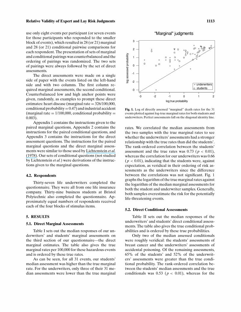
As can be seen, for all 31 events, our students’median assessment was higher than the true marginalrate. For the underwriters, only three of their 31 me-dian assessments were lower than the true marginal

-3 -2 -1 0 1 2

-3

-2

-1

0

1

2

3

log true probability

log

asse

ssed

pro

babi

lity

"Marginal" judgments

underwritersstudents

Fig. 1. Log of directly assessed “marginal” death rates for the 31events plotted against log-true marginal rates for both students andunderwriters. Perfect assessments fall on the diagonal identity line.

rates. We correlated the median assessments fromthe two samples with the true marginal rates to seewhether the underwriters’ assessments had a strongerrelationship with the true rates than did the students’.The rank-ordered correlation between the students’assessment and the true rates was 0.73 (p < 0.01),whereas the correlation for our underwriters was 0.66(p < 0.01), indicating that the students were, againstexpectation, as veridical in their ordering of risk as-sessments as the underwriters since the differencebetween the correlations was not significant. Fig. 1graphs the logarithm of the true marginal rates againstthe logarithm of the median marginal assessments forboth the student and underwriter samples. Generally,both samples overestimate the risk for the potentiallylife-threatening events.

5.2. Direct Conditional Assessments

Table II sets out the median responses of theunderwriters’ and students’ direct conditional assess-ments. The table also gives the true conditional prob-abilities and is ordered by these true probabilities.

Only two of the median assessed conditionalswere roughly veridical: the students’ assessments ofbreast cancer and the underwriters’ assessments ofaccidental poisoning. Of the remaining assessments,65% of the students’ and 52% of the underwrit-ers’ assessments were greater than the true condi-tional probability. The rank-ordered correlation be-tween the students’ median assessments and the trueconditionals was 0.53 (p < 0.01), whereas for the

1114 Wright, Bolger, and Rowe

0-1-2-3-4-5-6-7-8-9-10

0

-1

-2

-3

-4

-5

-6

-7

-8

log true probability

log

asse

ssed

pro

babi

lity

underwritersstudents

"Conditional" judgments

Fig. 2. Log of directly assessed “conditional” death rates for the 31events plotted against log-true conditional rates for both studentsand underwriters. Perfect assessments fall on the diagonal identityline.

underwriters it was 0.66 (p < 0.01). Although the un-derwriters’ performance was better than the students’on this aspect, these correlations were not found tobe significantly different from one another. Fig. 2graphs the logarithm of the true conditional probabil-ities against the logarithm of the median conditionalprobability assessments. Unlike the marginal assess-ments, there is no systematic bias of overestimation:the probability of some events was underestimatedand others overestimated.

5.3. Paired Assessments: Group Marginal Analysis

Fig. 3a graphs, on the y-axis, the students’ medianmarginal probabilities for each of the pairings of lethalevents within each of the four groupings of events, i.e.,there are 105 data points. These medians are for theassessed relative likelihood of death from the events,converted to half-range probabilities (i.e., 0.5 to 1.0),of the truly most likely event of a pair occurring. Thisvalue will approach 1.0 when “times more likely theevent you circled causes death” approaches infinity.For example, if the “times more likely” is 99, thenthe probability is 0.99. If the “times more likely” isthought to be 300, then the probability is 300 dividedby 301, which equals 0.99667, and so on. Values thatfall below 0.5 on the y-axis represent cases in which,on average, the respondents incorrectly identify themore likely cause of death. The number of dots abovethis line, in proportion to the number of dots below,shows the proportion of median responses that cor-

1.00.90.80.70.60.5

1.0

0.9

0.8

0.7

0.6

0.5

0.4

0.3

0.2

0.1

true relative probabilities

asse

ssed

rel

ativ

e pr

obab

ilitie

s

Students' marginal judgments

Fig. 3a. Students’ 105 pairwise assessments of “marginal” deathrates each expressed as a probability that the truly most likelyevent of each pair will lead to death relative to the truly least likelyevent of each pair. These assessed relative probabilities are plot-ted against the true relative probabilities calculated in the samemanner. Perfect assessments fall on the diagonal identity line andcorrect identifications of the truly most likely event of each pair fallabove the dashed horizontal line.

1.00.90.80.70.60.5

1.0

0.9

0.8

0.7

0.6

0.5

0.4

0.3

0.2

0.1

0.0

asse

ssed

rela

tive

pro

babi

litie

s

true relative probabilities

Underwriters' marginal judgments

Fig. 3b. Underwriters’ 105 pairwise assessments of “marginal”death rates each expressed as a probability that the truly mostlikely event of each pair will lead to death relative to the trulyleast likely event of each pair. Assessed relative probabilities areplotted against the true relative probabilities calculated in the samemanner. Perfect assessments fall on the diagonal identity line andcorrect identifications of the truly most likely event of each pair fallabove the dashed horizontal line.

rectly identified the truly most likely cause of deathfrom the pairing. On the x-axis, we plot the true half-range probability of each truly more likely event oc-curring, calculated in the same manner (such that allvalues lie between 0.5 and 1.0). Fig. 3b repeats this

Relative Validity of Expert and Lay Risk Judgments 1115

analysis for the underwriters. This analysis is anal-ogous to that shown in Lichtenstein et al.’s (1978).Figs. 2 and 3, with the exception that their “true ra-tio” x-axis is compressed here due to the half-rangeconversion of the relative likelihoods. Note that thefigures from Lichtenstein at al. (1978) plot true ratioagainst percentage correct.

As can be seen by visual inspection of the twofigures, both students and underwriters generally un-derestimate the relative likelihoods of the events,in that the relative median assessed likelihoods aregenerally lower than the true relative likelihoods (asindicated by the occurrence of most of the pointsbelow the diagonal in both figures). In other words,both groups of respondents do not appreciate the true(larger) differences in rates. This is particularly so incases where the true probability is high (that is, theratio in terms of number of deaths between the twolethal events is high). In short, both groups of respon-dents appear to be using compressed ranges of ratioestimates, resulting in over-homogenous estimations.If we consider the estimates that fall below a horizon-tal line drawn at 0.5 on the y-axis, then this indicatesoccasions in which the wrong option of a pair was,on average, estimated to be the more likely cause ofdeath. Application of chi-square tests on a two-by-twocontingency table, which was made by counting thenumber of points above and below the horizontal line(right and wrong) and to the left and right of 0.75 (lowand high), did not reach significance (chi-square =2.23, df = 1, NS; and chi-square = 2.75, df = 1, NS, forthe data shown in Fig. 3a and 3b, respectively). Thisresult contrasts with that of Lichtenstein et al. (1978)with both a student sample (their Fig. 2, page 555) andwith a sample of the League of Women Voters (theirFig. 3, page 557), where respondents were found tobe more likely to choose the wrong option when thetrue relative likelihood was low.

The rank-ordered correlations between assessedmedian marginals and true marginals was 0.24 (p <

0.05) for the students and 0.42 (p < 0.01) for the un-derwriters. Although the underwriters appeared bet-ter at judging the relative likelihood of pairs of events,the difference between correlations did not reach sig-nificance. It is interesting to note, however, that thistrend reverses that shown in the direct comparisons.

5.4. Paired Assessments: Group ConditionalAnalysis

Figs. 4a and 4b repeat the above analysis—thistime for paired conditional assessments. Both graphs

1.00.90.80.70.60.5

0.95

0.85

0.75

0.65

0.55

0.45

0.35

0.25

0.15

true relative probabilities

asse

ssed

rela

tive

pro

babi

litie

s

Students' conditional judgments

Fig. 4a. Students’ pairwise assessments (N = 105) of “conditional”death rates each expressed as a probability that the truly mostlikely event of each pair will lead to death relative to the trulyleast likely event of each pair. Assessed relative probabilities areplotted against the true relative probabilities calculated in the samemanner. Perfect assessments fall on the diagonal identity line andcorrect identifications of the truly most likely event of each pair fallabove the dashed horizontal line.

1.00.90.80.70.60.5

1.0

0.5

0.0

true relative probabilities

asse

ssed

rel

ativ

e pr

obab

ilitie

s

Underwriters' conditional judgments

Fig. 4b. Underwriters’ pairwise assessments (N = 105) of “condi-tional” death rates each expressed as a probability that the trulymost likely event of each pair will lead to death relative to the trulyleast likely event of each pair. Assessed relative probabilities areplotted against the true relative probabilities calculated in the samemanner. Perfect assessments fall on the diagonal identity line andcorrect identifications of the truly most likely event of each pair fallabove the dashed horizontal line.

again evidence general underestimation of the truedifference between pairs of events, this time in termsof their relative lethality. As previously, the tendencyto choose the wrong option as more lethal appearsto be associated with a smaller real difference in the

1116 Wright, Bolger, and Rowe

likelihood ratio between pairs. The rank-ordered cor-relations between assessments and true values were0.25 (p < 0.05) and 0.42 (p < 0.01) for the studentsand the underwriters, respectively. Again, the under-writers appeared to be better, although the differencebetween these correlations was nonsignificant.

5.5. Paired Assessments: Individual Analysis

As outlined earlier, each respondent made ei-ther 28 or 21 paired marginal assessments within oneblock of life-threatening event items. This richness ofdata—at the level of the individual respondent—allowed us to measure an individual’s error over hisor her total number of assessments. For each respon-dent, we computed the mean average percentage er-ror (MAPE), which is defined as:

i=n∑

i=1abs

( ai −titi

)

n∗ 100%

where ai = assessed relative probability of the trulymost likely event of a pair occurring; n = the numberof paired assessments made by an individual; and ti =true relative probability of that event occurring.

The overall mean MAPEs for the marginal pair-ings were 42.7 (SD 11.3) and 36.4 (SD 8.2) for ourstudents and underwriters, respectively. The meanswere significantly different (t = 2.35, df = 73, p <

0.05, two-tailed). Turning now to the conditional pair-ings, the overall mean MAPEs were 45.4 (SD 11.0)and 38.7 (SD 8.7) for our students and the underwrit-ers, respectively. The difference between the meansdid reach significance (t = 2.49, df = 73, p < 0.05).Clearly, our underwriters were more accurate in theirpaired assessments than our undergraduate students,but only by a factor of, roughly, six percentage pointsof error.

Within our paired comparison data, we were alsoable to derive a measure of the reliability of an in-dividual’s assessments. Our analysis focused on thenumber of inconsistent triads within an individual’spaired comparisons. For example, if an individualstates that lethal event “a” is more likely than lethalevent “b” and also that lethal event “b” is more likelythan lethal event “c,” he or she should not state thatlethal event “c” is more likely than lethal event “a.”Within the blocks of 28 paired comparisons, the max-imum possible number of such inconsistent triads is20. Within the block of 21 paired comparisons, themaximum possible number of inconsistent triads is 14.For the marginal pairwise comparisons, our students

averaged 15% of inconsistent triads, whereas our un-derwriters averaged 18%. Nonparametric analysis re-vealed that this difference was not significant (MannWhitney u = 315, p > 0.05, two-tailed). For the con-ditional pairwise comparisons, the average number ofinconsistent triads was 8% for both samples. No sig-nificant correlations were obtained between individ-uals’ degree of inconsistency and subsequent overallMAPE in either the marginal or conditional sectionsof our sets of paired comparisons, within our samplesof students and underwriters.

5.6. Underwriting Experience and PairedAssessments

Our underwriters also provided individual bio-graphical data on: the number of years that they hadworked at the particular insurance company (x̄ =6.13, SD = 6.21), the approximate number of yearsthey had been doing life underwriting (x̄ = 3.65, SD =4.71), the approximate number of hours they spenteach week on underwriting (x̄ = 11.74, SD = 12.33),the approximate number of proposals they assessedper week (x̄ = 54.4, SD = 43.7), and the discretionaryband within which they were able to make proposalevaluations without referral to a more senior under-writer. These bands were: (1) up to £30,000 withno additional evidence from that contained on theproposal form, (2) up to £50,000 with no evidence,(3) any proposal, no evidence, (4) up to £100,000 atordinary rates but with additionally provided medicaland other evidence on the risk, (5) up to £200,000with evidence and the discretion to charge addi-tional premiums, (6) up to £300,000 with evidenceand discretion, and (7) any proposal within the com-pany’s limits. We coded these discretionary bands as1 through 7. The frequency with which the underwrit-ers fell into these bands was, 3, 3, 8, 5, 6, 9, and 3,respectively.

Our next analysis was to correlate our individualmeasures of underwriting experience with our indi-vidual measures of marginal/conditional and incon-sistent triads. Our nonparametric correlation matrixis set out in Table III.

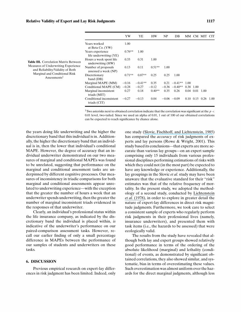
Several of the obtained significant correlationsare unsurprising. For example, the higher the discre-tion of underwriting band that an individual is in, thelonger he or she has worked at the insurance company,and the longer the number of years that he or shehas been doing life underwriting. Some of the otherobtained correlations are perhaps less obvious: thelower the individual’s marginal MAPE, the greater

Relative Validity of Expert and Lay Risk Judgments 1117

Table III. Correlation Matrix BetweenMeasures of Underwriting Experience

and Reliability/Validity of BothMarginal and Conditional Risk

Assessments1

YW YE HW NP DB MM CM MIT CIT

Years worked 1.00at Beta Co. (YW)

Years experience 0.76** 1.00life underwriting (YE)

Hours a week spent life 0.33 0.31 1.00underwriting (HW)

Number of proposals 0.13 0.11 0.51** 1.00assessed a week (NP)

Discretionary 0.71** 0.87** 0.25 0.25 1.00band (DB)

Marginal MAPE (MM) −0.16 −0.41** 0.35 0.21 −0.41** 1.00Conditional MAPE (CM) −0.28 −0.27 −0.12 −0.36 −0.40** 0.38 1.00Marginal inconsistent 0.27 0.18 0.40** 0.35 0.26 0.04 0.01 1.00

triads (MIT)Conditional inconsistent −0.27 −0.13 0.04 −0.06 −0.09 0.10 0.15 0.26 1.00

triads (CIT)

1Two asterisks next to obtained correlation indicate that the correlation was significant at the p <

0.01 level, two-tailed. Since we used an alpha of 0.01, 1 out of 100 of our obtained correlationscan be expected to reach significance by chance alone.

the years doing life underwriting and the higher thediscretionary band that this individual is in. Addition-ally, the higher the discretionary band that an individ-ual is in, then the lower that individual’s conditionalMAPE. However, the degree of accuracy that an in-dividual underwriter demonstrated on our two mea-sures of marginal and conditional MAPEs was foundto be unrelated, suggesting that performance on themarginal and conditional assessment tasks are un-derpinned by different cognitive processes. Our mea-sures of inconsistency in triadic comparisons for bothmarginal and conditional assessments appear unre-lated to underwriting experience—with the exceptionthat the greater the number of hours a week that anunderwriter spends underwriting, then the greater thenumber of marginal inconsistent triads evidenced inthe responses of that underwriter.

Clearly, an individual’s professional status withinthe life insurance company, as indicated by the dis-cretionary band the individual is placed within, isindicative of the underwriter’s performance on ourpaired-comparison assessment tasks. However, re-call our earlier finding of only a small percentagedifference in MAPEs between the performance ofour samples of students and underwriters on thesetasks.

6. DISCUSSION

Previous empirical research on expert-lay differ-ences in risk judgment has been limited. Indeed, only

one study (Slovic, Fischhoff, and Lichtenstein, 1985)has compared the accuracy of risk judgments of ex-perts and lay persons (Rowe & Wright, 2001). Thisstudy based its conclusions—that experts are more ac-curate than various lay groups—on an expert samplecomprising only 15 individuals from various profes-sional disciplines performing estimations of risks withwhich they could not (in the most part) be expected tohave any knowledge or experience. Additionally, thelay groupings in the Slovic et al. study may have beenunaware that the evaluative standard for their “risk”estimates was that of the relative frequency of mor-tality. In the present study, we adopted the method-ology of a second study, conducted by Lichtensteinet al. (1978), in order to explore in greater detail thenature of expert-lay differences in direct risk magni-tude judgments. Furthermore, we took care to selecta consistent sample of experts who regularly performrisk judgments in their professional lives (namely,insurance underwriters), and presented them withtask items (i.e., the hazards to be assessed) that wereecologically valid.

The results from the study have revealed that al-though both lay and expert groups showed relativelygood performance in terms of the ordering of theabsolute likelihood (marginal) and lethality (condi-tional) of events, as demonstrated by significant ob-tained correlations, they also showed similar, and sys-tematic, bias in terms of overestimating these values.Such overestimation was almost uniform over the haz-ards for the direct marginal judgments, although less

1118 Wright, Bolger, and Rowe

so for conditionals. The student group was no worse atdirect marginal or direct conditional estimation thanthe experts.8

Because the direct estimation of risks associatedwith potentially lethal events is an unusual task, evenfor our experts (at least for marginal estimates, al-though for conditional estimates the Chief Under-writer stated that this assessment mode captured theessence of her work-a-day task), we also obtainedmarginal and conditional estimates in a second, indi-rect way, namely, through pairwise comparisons. Cor-relational analysis revealed a trend that the expertswere indeed better at the task, in terms of identi-fying which events of the pairs led to more deaths(marginals) and were more lethal (conditionals), al-though these correlations were not significantly dif-ferent from those of the lay group. However, analysisof MAPEs revealed that the experts did make signifi-cantly better judgments than lay persons on marginalestimates in terms of ratios (i.e., the number of timesone event was more likely to cause death than an-other), and conditionals (i.e., the number of times anevent was more likely to cause death than the other,given that the event happens to someone). In spite ofthis, both lay persons and experts made the same gen-eral errors in the pairwise comparison tasks, namely,in underestimating the ratio of more-to-less ubiqui-tous and fatal hazards, that is, in overly compressingtheir ranges of estimates.

So what do these results mean? The experts were,generally, a little better in their risk judgments thanthe lay persons, and the fact that expertise did makesome difference was shown by the finding that themore senior underwriters made lower errors (in termsof MAPEs) in both the pairwise marginal and con-ditional tasks than those that were less senior. Butthe differences in performance between experts andlay persons were small in magnitude, and the na-ture of the biases (in terms of overestimating di-rect estimates and underestimating the differencesin marginal/conditional riskiness between pairs ofevents), were common to both groups. These gen-

8 Expert-novice differences would be expected to be fairly large ifthey are to be at all practically relevant, in which case our sam-ple size, although fairly small, should be adequate to achieve areasonable level of power (0.8 or above, as suggested by Cohen,1977). If this is the case, then, on the basis of our nonsignificantresults, we can say our experts are mostly not doing any betterthan the novices (despite the confident responses of the ChiefUnderwriter to the contrary).

eral biases seem to revolve around inadequate scal-ing of estimates, which is unsurprising, at least in thecase of the lay group, given unfamiliarity with the rawfigures related to risk. But why were the experts nobetter?

The previous evidence for experts being betterat the judgments of risks (and, indeed, of perceiv-ing risks in a different way than do lay persons) isnot strong (see Rowe & Wright, 2001, for a review),and yet has been so readily accepted that there hasbeen no apparent effort to research the topic fur-ther. For “true” expertise to be manifest (expertiserelated to performance, as opposed to social and po-litical imperatives), Bolger and Wright (1994) haveargued that the expert must perform a task that isecologically valid, and the task must also be learn-able. We attempted to ensure that our expert-taskmatch was as strong as possible (given experimentallimitations), and that ecological validity was high, andyet we still obtained expert performance that was notmuch better than lay person performance. This resultsuggests that the underwriting task is not truly “learn-able,” i.e., it is not one for which there is regular feed-back on the correctness or otherwise of judgments.Indeed, in the training of underwriters, performanceis assessed according to the similarity of junior under-writers’ judgments to those of their seniors (Bolgeret al., 1989). Once “trained,” underwriters receiveinfrequent performance-related, objective feedbackabout the correctness of their judgments and indeedit would be difficult to provide such feedback, giventhat a “poor” judgment might turn out to be insuringan applicant who subsequently died of a conditionafter, perhaps, 20 years of a 25-year policy.

We infer that the tasks performed by other pro-fessional risk assessors may also be unlearnable. Forexample, in the case of major hazards in the nuclearindustry there may be no risk/judgment feedback atall. From this, we suggest that expert-lay differencesin the accuracy of such risk judgments, or in the natureof such judgments (given that the biases evidenced inthis study were similar across lay and expert groups),cannot be assumed. Further, even if experts are sig-nificantly more accurate than lay people, it may stillbe that differences in accuracy are small, as demon-strated in the present study. Perhaps the common-sense assumption of the superiority of expert riskassessors in making risk judgments is ill founded. Cer-tainly, future research needs to pay more attention tothe de facto nature of the learnability of tasks per-formed by professional risk assessors.

Relative Validity of Expert and Lay Risk Judgments 1119

APPENDIX 1

Instructions

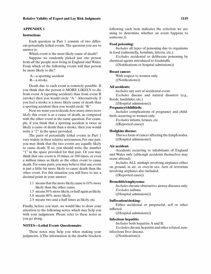
Each question in Part 1 consists of two differ-ent potentially lethal events. The question you are toanswer is:

Which event is the most likely cause of death?Suppose we randomly picked just one person

from all the people now living in England and Wales.From which of the following events will that personbe more likely to die?

A—a sporting accidentB—a stroke

Death due to each event is remotely possible. Ifyou think that the person is MORE LIKELY to diefrom event A (sporting accident) than from event B(stroke) then you would circle “A.” Alternatively, ifyou feel a stroke is a more likely cause of death thana sporting accident then you would circle “B.”

Next we want you to decide how many times morelikely this event is as a cause of death, as comparedwith the other event in the same question. For exam-ple, if you think that a sporting accident is twice aslikely a cause of death than a stroke, then you wouldwrite a “2” in the space provided.

The pairs of potentially lethal events in Part 1vary widely in their relative seriousness. For one pair,you may think that the two events are equally likelyto cause death. If so, you should write the number“1” in the space provided for that pair. Or you maythink that one event is 10 times, or 100 times, or evena million times as likely as the other event to causedeath. For some pairs, you may believe that one eventis just a little bit more likely to cause death than theother event. For this situation you will have to use adecimal point in your answer:

1.1 means that the more likely cause is 10% morelikely than the other cause.

1.5 means 50% more likely, or half again as likely.1.8 means 80% more likely.2.5 means two and a half times as likely, etc.

Finally, before you start, we would like to draw yourattention to the following notes, which may help youwith your judgments. Please refer to these notes asyou go along.

NOTES—Lethal Events Questionnaire

These notes may help you when making yourjudgments. ((The information in the double brackets

following each item indicates the criterion we areusing to determine whether an event happens tosomeone.))

Food poisoning:Includes all types of poisoning due to organisms

in food (salmonella, botulism, listeria, etc.).Excludes accidental or deliberate poisoning by

chemical agents introduced to foodstuffs.((Notifications or hospital admissions))

Breast cancer:With respect to women only.((Notifications))

All accidents:Includes any sort of accidental event.Excludes disease and natural disasters (e.g.,

floods, landslides, etc.).((Hospital admissions))

Pregnancy/childbirth:Includes complications of pregnancy and child-

birth occurring to women only.Excludes infants, fetuses, etc.((Reported cases))

Hodgkins disease:This is a form of cancer affecting the lymph nodes.((Hospital admissions))

Air accident:Accidents occurring to inhabitants of England

and Wales only (although accidents themselves mayoccur abroad).

Includes ALL mishaps involving airplanes eitheron ground, in air, or over/in sea. Acts of terrorisminvolving airplanes also included.

((Reported cases))

Bronchitis/emphysema:Includes chronic obstructive airway diseases only.Excludes asthma.((Hospital admissions))

Suffocation/choking:Either accidental or purposeful, self or other

inflicted.((Hospital admissions))

Infectious hepatitis:Includes both hepatitis A and B.Excludes chronic hepatitis and other related, non-

infectious liver disease.((Notifications))

1120 Wright, Bolger, and Rowe

Domestic accident:Includes mishaps in and around the house.Excludes diseases and violent acts.((Hospital admissions))

Whooping cough:Infectious disease.((Notifications))

Lung cancer:Includes cancer of the lungs only.Excludes cancer of oesophagus, throat, etc.((Notifications))

Diabetes:Disorder of process by which the body uses sugars

and other carbohydrates.((Diagnoses))

Rail accident:Includes train collisions only.Excludes falls from train, person on track, etc.((Reported cases))

Accidental poisoning:Includes chemical substances taken unintention-

ally.Excludes organic poisoning by foodstuffs and pur-

poseful administration of harmful substances.((Hospital admissions))

Alcohol/drugs:Includes all substances purposely taken except as

a means of suicide.Excludes substances taken accidentally or for

medical purposes.((Hospital and special unit admissions))

Measles:Infectious disease.((Notifications))

Fire and flames:Includes burns and smoke inhalation only.((Hospital admissions))

Asthma:Includes both allergic and late-onset asthmas.Excludes other obstructive airway diseases such

as bronchitis and emphysema.((Hospital admissions))

Polio:Infectious disease of the nervous system.((Notifications))

Stomach cancer:Includes cancer of alimentary tract, oesophagus,

and intestines, as well as stomach.((Notifications))

Car accident:Includes passengers and drivers of any motor ve-

hicle (cars, buses, motorcycles, lorries, etc.).Excludes cyclists and pedestrians.((Reported severities))

Smoking related:Includes deaths due to lung cancer, heart disease,

and respiratory diseases attributable to active smok-ing only.

((Estimated proportion of admissions/notifica-tions of above three ailments))

Salmonella:Bacterial food poisoning.((Reported cases))

Leukaemia:Acute and chronic cancers characterized by an

abnormal increase in the number of white blood cells.Excludes other, noncancerous blood diseases.((Notification))

Lightning:Act of God!((Reported cases))

Hypertension:Includes high blood pressure due to underly-

ing pathology (e.g., kidney disease, hardening of thearteries, etc.).

Excludes high blood pressure with no knowncause and temporarily elevated blood pressure dueto, e.g., exertion.

((Hospital admissions))

Meningitis:Infectious disease of the nervous system.((Notifications))

Road accident:Includes pedestrians and cyclists hit by motor

vehicles.Excludes drivers and passengers of motor

vehicles.((Reported severities))

Benign tumors:Includes tumors classified as “benign” due to

location and/or noninvasive nature (i.e., nonspread-ing).

Excludes tumors classified as “malignant” and be-nign tumors later reclassified as malignant.

((Notifications))

Relative Validity of Expert and Lay Risk Judgments 1121

Electric shock:Shock from mains voltages or higher.((Reported cases))

APPENDIX 2

Instructions

In Part 1 we asked you to judge the relative like-lihood of death from pairs of events.

In Part 2 we would like you to judge the samepairs of events BUT this time we would like you toanswer:

Which event is the most likely to cause deathgiven it happens to someone?

Suppose we randomly picked just one personfrom all the people now living in England and Wales.Let’s say, for example, that one of the two followingpotentially lethal events happens to this person:

A—he or she is involved in a motorcycle accidentB—he or she is diagnosed as having influenza

If you think the person is MORE LIKELY todie as a result of event A (motorcycle accident) thanas a consequence of event B (influenza) then youwould circle “A.” Alternatively, if you feel influenzahas more serious consequences in terms of mortalitythan a motorcycle accident, then you would circle “B.”

Next we want you to decide how many times morelikely this event is to cause death, as compared withthe other event given in the same question. For ex-ample, if you think flu is twice as likely to cause deathto someone than him or her being involved in a mo-torcycle accident, then you would write a “2” in thespace provided.

Please mark your judgments in a similar man-ner to the way you did in Part 1 (i.e., “1” meansequally likely, “1.5” means 50% more likely, “2”means twice as likely, “100” means 100 times morelikely, “1,000,000” a million times more likely, etc.).

Again you may refer to the notes relating to eachevent that are given in Part 1.

APPENDIX 3

Instructions

What you have been judging in Parts 1 and 2 arewhat are known as marginal and conditional probabil-ities of death due to various potentially lethal events.

The marginal probability in this case refers to thenumber of people dying in England and Wales eachyear as the result of a particular lethal event.

For example, in 1986 in England and Wales163,200 died as a result of heart disease (excludingstroke).

This is normally expressed as a mortality rate, e.g.,326/100,000 for the heart disease example above.

Thus 326 people out of every 100,000 in the entirepopulation of England and Wales died as a result ofheart disease in 1986.

The conditional probability in this case refers tothe likelihood of someone dying in England and Waleseach year given that a particular event has happenedto them.

For example, in 1986 in England and Wales348,718 people were admitted to hospital with diag-nosed heart disease (excluding stroke).

As we know from the marginal probability above,163,200 people actually died of heart disease that year.Assuming (as appears to be the case) that the num-ber of fatalities and hospital admissions remains fairlyconstant over years for heart disease, we can estimatethe likelihood of death from heart disease for some-one diagnosed as suffering from this ailment.

This means that just under half the people whosuffer from heart disease subsequently die from it.If the conditional probability had been 1 this wouldmean that all people suffering from heart disease dieas a result of it. If the conditional probability had been0 this would mean that no people suffering from heartdisease die as a consequence of that ailment.

It has been found that people give very differentestimates of marginal and conditional probabilitiesfor the same events, depending on how these proba-bilities for the same events are asked for. Generally,people seem to find it easiest to give estimates in theform of the paired comparisons you made in Parts 1and 2. However, we would also like you to try and givedirect estimates of the marginal and conditional val-ues for each of the lethal events you have previouslyconsidered.

REFERENCES

Barke, R. P., & Jenkins-Smith, H. C. (1993). Politics and scientificexpertise: Scientists, risk perception, and nuclear waste policy.Risk Analysis, 13(4), 425–439.

Bolger, F., & Wright, G. (1994). Assessing the quality of expertjudgment: Issues and analysis. Decision Support Systems, 11,1–24.

Bolger, F., Wright, G., Rowe, G., Gammack, J., & Wood, B. (1989).LUST for life: Developing expert systems for life assuranceunderwriting. In N. Shadbolt (Ed.), Research and developmentin expert systems VI. Cambridge: CUP.

Cohen, J. (1977). Statistical power analysis for the behavioral sci-ences. New York: Academic Press.

1122 Wright, Bolger, and Rowe

Einhorn, H. J. (1980). Learning from experience and suboptimalrules in decision making. In T. Wallsten (Ed.), Cognitive pro-cesses in choice and decision (pp. 1–20). Hillsdale, NJ: Erlbaum.

Flynn, J., Slovic, P., & Mertz, C. K. (1993). Decidedly different: Ex-pert and public views of risks from a radioactive waste reposi-tory. Risk Analysis, 13(6), 643–648.

Gutteling, J. M., & Kuttschreuter, M. (1999). The millennium bugcontroversy in the Netherlands? Experts’ views versus publicperception. In L. H. J. Goossens (Ed.), Proceedings of the 9thannual conference of risk analysis: Facing the millennium (pp.489–493). Delft: Delft University Press.

Keren, G. (1987). Facing uncertainty in the game of bridge: A cal-ibration study. Organizational Behavior and Human DecisionProcesses, 39, 98–114.

Kraus, N., Malmfors, T., & Slovic, P. (1992). Intuitive toxicology: Ex-pert and lay judgments of chemical risks. Risk Analysis, 12(2),215–232.

Lichtenstein, S., Slovic, P., Fischhoff, B., Layman, M., & Combs, B.(1978). Judged frequency of lethal events. Journal of Experi-mental Psychology: Human Learning and Memory, 4, 551–578.

Maxwell, R. J. (1999). The British government’s handling of risk:Some reflections on the BSE/CJD crisis. In P. Bennett & K.Calman (Eds.), Communications and public health (pp. 94–107). Oxford: Oxford University Press.

McDaniels, T. L., Axelrod, L. J., Cavanagh, N. S., & Slovic, P. (1997).Perception of ecological risk to water environments. Risk Anal-ysis, 17(3), 341–352.

Mumpower, J. L., Livingston, S., & Lee, T. J. (1987). Expert judg-ments of political riskiness. Journal of Forecasting, 6, 51–65.

Murphy, A. H., & Brown, B. G. (1985). A comparative evaluation ofobjective and subjective weather forecasts in the United States.In G. Wright (Ed.), Behavioural decision making. New York:Plenum.

Rowe, G., & Wright, G. (2001). Differences in experts and layjudgments of risk: Myth or reality? Risk Analysis, 21, 341–356.

Rowe, G., & Wright, G. (1993). Expert systems in insurance: Areview and analysis. International Journal of Intelligent Systemsin Accounting, Finance, and Management, 2, 129–145.

Shanteau, J. (1978). When does a response error become a judgmen-tal bias? Commentary on “Judged frequency of lethal events”.Journal of Experimental Psychology: Human Learning andMemory, 4(6), 579–581.

Slovic, P. (1987). Perception of risk. Science, 236, 280–285.Slovic, P. (1999). Trust, emotion, sex, politics and science: Surveying

the risk-assessment battlefield. Risk Analysis, 19(4), 689–701.Slovic, P., Fischhoff, B., & Lichtenstein, S. (1985). Characteriz-

ing perceived risk. In R. W. Kates, C. Hohenemser, & J. X.Kasperson (Eds.), Perilous progress: Managing the hazards oftechnology (pp. 91–125). Boulder, CO: Westview.

Slovic, P., Malmfors, T., Krewski, D., Mertz, C. K., Neil, N., &Bartlett, S. (1995). Intuitive toxicology II. Expert and lay judg-ments of chemical risks in Canada. Risk Analysis, 15(6), 661–675.

Wright, G., Pearman, A., & Yardley, K. (2000). Risk percep-tion in the UK oil and gas production industry: Are expertloss-prevention managers’ perceptions different from those ofmembers of the public? Risk Analysis, 20, 681–690.