\AN EMPIRICAL CONSTITUTIVE EQUATION FOR ANTI ...

\AN EMPIRICAL CONSTITUTIVE EQUATION

FOR ANTI-COAGULATED HUMAN BLOOD,

by

Frederick James, Walburn;

Thesis submitted to the Graduate Faculty of the

Virginia Polytechnic Institute and State University

in partial fulfillment of the requirements for the degree of

MASTER OF SCIENCE

in

Engineering Science and Mechanics

APPROVED:

J ; D. J. Schneck, Chairman

H. F. Brinson D. Frederick

e “s ;

€, Kee'sap, . oO C. Os borers

J. E. Kaiser a ts J. C. Osborne

April, 1975

Blacksburg, Virginia

ACKNOWLEDGMENTS

My first wish is to express my deepest appreciation to Dr. Daniel

J. Schneck of the Engineering Science and Mechanics Department,

Virginia Polytechnic Institute and State University for his guidance,

encouragement, and most of all, introducing to me a fascinating field

of study. I wish to thank Dr. J. E. Kaiser, Dr. H. F. Brinson, and

Dr. D. Frederick of the same department and Dr. J. C. Osborne of the

Veterinary Science Department for serving as members of my graduate

committee. I am also grateful for the assistance provided by my aunt,

Miss Marjorie Walburn and the statistical advice of Ms. Agnes Heller is

appreciated. I wish to thank all connected with the Montgomery County

Hospital, especially Jim Mitchell and all others who work in the

hemotology lab, for the donation of the blood samples used in this

study. Thanks also go to Dr. William Gutstein of New York Medical

College for providing the total lipid determinations. I wish to

thank Willie Mae Hylton for an excellent job of typing this thesis.

Finally I wish to express my appreciation to my parents, Mr. and Mrs.

James H. Walburn, for their financial and spiritual assistance and I

dedicate this thesis to them.

Li

TABLE OF CONTENTS

ACKNOWLEDGMENTS ° e ® C4 s s e e » e * e » ° s e . e * e e e e e ii

LIS T OF F IGURE S * ® e * ° » ° e s ° i] * e ° ° » ° e e . » * e e Vv

LIST OF TABLES * e e a « ° e e e e e s e e ® e * s . e e ° * ° ® vii

CHAPTER

I. INTRODUCTION . . 2 5 © © © © © © © © ow ow te ew oe oe 1

IIT. REVIEW OF LITERATURE . 2. 2. « «© © © © © © © © ew ww ow 3

A. Early Work . . 2. 2. 6 © «© © © © we wo ew ew we ew we 3

B. Modern Developments ... « »« « © © «© » «© © © © 4

C. Summary ... «6 «© © © © © © © © we ew eh we 8

III. THE PRESENT PROBLEM . 2. « 2 «© © © © » © © © © ow ww 10

IV. METHOD OF ANALYSIS . . 2. 2. «© «© © © © we we we we wwe we 11

A. Materials . . 2. «6 2 © © © © © ew we ew we ee ww 1

B. Variables . 2. 2 2 0 0 2 ee ew ww ww we ew tw ww 12

C. Statistical Analysis ...... 2. «© © e we we wo 12

V. RESULTS AND DISCUSSION . 2. 1. 4 6 © 0 ee © we we ew ow 17

A. Preliminary Remarks »- © © © © © © © © © © © 8» @© @ 17

B. Dependence on Hematocrit . .. . 2 «© « © «© « © « 18

C. Dependence on Plasma Proteins . ..... «see. 20

D. Dependence on Plasma Lipids ..... 0 © «© © «© « 25

VI. SUMMARY AND CONCLUSIONS . .. 2. 6 © «© © © © © wo wo we ow 27

A. Constitutive Equations Devetoped ......e«- 27

B. Results Summarized and Conclusions .....».e 29

Lit

iv

TABLE OF CONTENTS - continued

C. Direction of Future Studies

REFERENCES , . 2. «6 © + © © © © wo

FIGURES 2. 2. 6 6 1 © © ew ew ew we ew

TABLES . 2. 2 © © 6 © ew wt ew ew

APPENDIX A--ON BLOOD... .. +e

APPENDIX B--NON-NEWTONIAN FLUIDS AND

APPENDIX C--WELLS-BROOKFIELD THEORY

APPENDIX D--THE R-SQUARE STATISTIC .

VITA 2. 1 wo ew we ww ew we we tw tw

ABSTRACT

°

°

30

31

37

63

67

68

75

82

91

10.

ll.

12.

13.

14.

15.

16.

17.

18.

19.

LIST OF FIGURES

Newtonian Velocity Profile ....

Types of Non-Newtonian Fluids...

A Pseudoplastic Fluid . ..... .

Behavior of a Time Dependent Fluid

Behavior of a Time Dependent Fluid

Hysteresis Loops . . «4+ « «ee

Hysteresis Loops .. ..« - «6 «6 « «

Power Law Equation with a Yield Stress

Cone Configuration ... +. «eo -

Velocity Distribution between the Cone and Plate

Bottom View of the Cone .....e-.

A True Equation and a Regression Equation .

The One Variable Model and Two Experimental Curves

A Comparison of the Non-Newtonian Index vs.

A Comparison of the Consistency Index vs. Hematocrit

for the Best Two Variable Model and Sacks! Model

A Comparison of the Consistency Index vs. Hematocrit for the Best Two Variable Model and the Best Three

Variable Model . ... 2 «© « we we

The Best Two and Three Variable Models at

Hamatocrit Level of 35%... ..-.

The Best Two and Three Variable Models at

Hematocrit Level of 38% . . «. « « -»

The Best Two and Three Variable Models at

Hematocrit Level of 41% . ... es.

*

a

D

Hematocrit

for the Best Two Variable Model and Sacks' Model

38

39

40

41

42

43

44

45

46

47

48

49

50

51

52

53

54

55

56

vi

LIST OF FIGURES - continued

Figure

20.

21.

22.

23.

24.

25.

The Best Two and

Hematocrit Level of 44%

The Best Two and

Hematocrit Level of 47%

The Best Two and Three Variable Models at

Hematocrit Level of 50%

The Best Three Variable Model at a Total Protein

Minus Albumin Level of 1.5 gm/100 m.

The Best Three Variable Model with a High and Low Value of Total Protein minus Albumin

* e

. t

°

®

Three Variable Models at

Three Variable Models at

Compared with the Best Two Variable Model .

The Best Two Variable Model and the Best Three

Variable Moded at an Intermediate Value of Total

Protein minus Albumin .

a °

a7

58

39

60

61

62

Table

Il.

Iil.

LIST OF TABLES

Page

Values of C, Cc, » and C, for Sacks' Model and the Best Two " vaFiable wedel ee ee ew we te tw tl tl tll 64

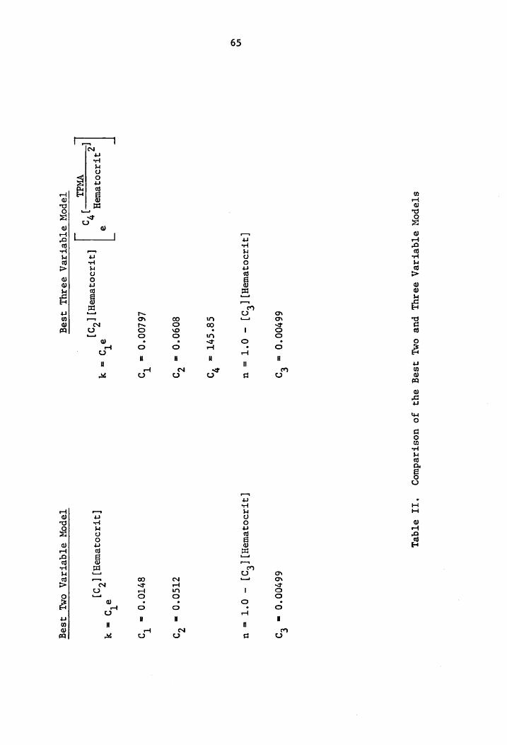
A Comparison of the Best Two and Three Variable Models e e ® a ° ¢ e e e e » » e e e s * e e e e ® e e s 65

Some Values of the Additional Term in the Best

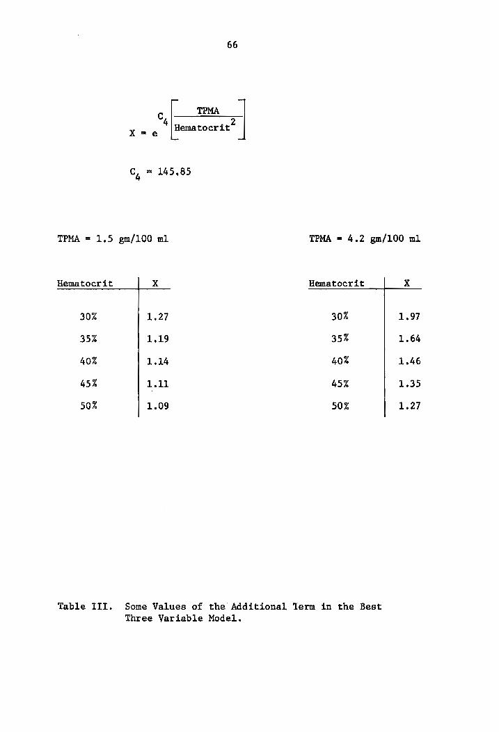
Three Variable Model ......-+ «© «© «© © © © © © © @ 66

vii

CHAPTER I

Introduction

Blood has always aroused wonder and curiosity in the mind of

man. Long ago on the ancient battlefields of Greece and Persia, men

marveled and wrote about this dark red fluid that oozed from some

wounds and spurted from others. In each case, death came to those

who had lost too much of this fluid, and so ancient scholars called

it The Fluid of Life, declaring that it was of the utmost importance

to the health of an individual. Galen, who lived from approximately

130 A.D. to 200 A.D., believed that all substances which entered the

body (food, air, etc.) were changed into blood, which then flowed to

different parts of the body where it was transformed into bones, skin,

hair, etc. This theory lasted for nearly fifteen hundred years [1].

Through the ages many noted scholars have studied blood [2],

among them Hippocrates (460-375 B.C.), Aristotle (384-322 B.C.),

Leonardo da Vinci (1452-1519 A.D.), Sir William Harvey (1578-1657

A.D.), Reverend Steven Hales (1733 A.D.), and a name familiar to many

engineers, Jean L. M. Poiseuille (1828 A.D.). This interest has con-

tinued, and today many investigators are studying the complex role of

blood in the cardiovascular system of man and animals. Yet, even with

the modern sophisticated research methods available today, there is

still much that is not known about this extremely complicated life-

giving fluid. Recently, investigators in both the medical and

engineering fields have found evidence which suggests that the

dynamics of blood flow in the cardiovascular system may be related to

arteriosclerosis. Commonly known as “hardening of the artery,"

arteriosclerosis is the number one killer in this country. Current

medical treatment of a heart attack or stroke, the most common con-

sequence of hardening of the arteries, is limited to saving the life

and then rehabilitating the patient. Until recently all really signi-

ficant advances have been concerned with the individual who already

has a discernible arteriosclerotic condition. Very little is known

about the specific causes of the disease. In order to uncover infor-

mation concerning the etiology of arteriosclerosis as related to

hemodynamics, two approaches could be utilized. The first is experi-

mental, where either an in vitro model of the in vivo flow situation

is constructed, and relevant information is obtained from the model,

or where the information is obtained directly from an animal.

The second approach is to develop a mathematical model of the

in vivo flow situation. Such a model for an incompressible fluid con-

sists of an equation of continuity (conservation of mass), three

generalized momentum equations, and a constitutive equation. When the

constitutive equation is introduced into the generalized momentum

equations, they become specific for the particular fluid involved in

the flow situation. With appropriate simplifications and boundary

conditions, the equation of continuity and the specific momentum

equations can be solved to yield information about the flow: stresses,

strain rates, etc. In accordance with the second approach, this thesis

offers an empirical constitutive equation for use in describing the

behavior of blood.

CHAPTER II

Review of Literature

A. Early Work

Interest in the viscosity of blood began in the early part of

this century when Hess [3] developed a simple convenient viscometer.

Of the many papers published during this period, however, it is

difficult to determine whether the investigator used whole blood,

plasma, or serum (see appendix A for definitions of physiologic terms).

Where whole blood was used, it is often further uncertain as to the

kind and quantity of anticoagulant that was used. Moreover, visco-

meters were of crude design and virtually every investigator used a

viscometer that was different from many others. Although it is

difficult to draw conclusions from this early work, some gross observa-

tions may be of value.

Fahraeus [4-6], Holker [7], and others [8-17] reported that

the viscosity of serum was increased in certain diseases. This proved

to be important, since serum or plasma viscosity could then be used to

measure the severity of a disease. In 1940, for example, T'ang and

Wang [18] found a good correlation between the increase in plasma

viscosity and the severity of a tuberculosis condition. Whittington

{19] and others [20-23] extended this work to other physiologic dis-

orders. Although much was done by these early investigators, the

crudeness and uncertainties cited above make their observations use-

ful only in a very general and qualitative way.

B. Modern Developments

For the most part, beginning in 1828 when the physiologist

Jean L. M. Pouiseuille [2] examined the steady laminar flow of water,

interest in the viscosity of whole blood, plasma, and serum centered

primarily around its relation to disease conditions. Investigators

simply accepted the fluid as being essentially Newtonian for their

purposes [24-34]. Inasmuch as the validity of using Stokes' Viscosity

Law for flow conditions characteristic of the cardiovascular system

has been seriously questioned [27], only recently has interest sur-

faced in actually determining a constitutive equation (see appendix

B) for the fluid.

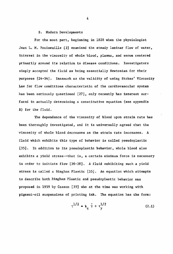
The dependence of the viscosity of blood upon strain rate has

been thoroughly investigated, and it is universally agreed that the

viscosity of whole blood decreases as the strain rate increases. A

fluid which exhibits this type of behavior is called pseudoplastic

[35]. In addition to its pseudoplastic behavior, whole blood also

exhibits a yield stress--that is, a certain minimum force is necessary

in order to initiate flow [36-38]. A fluid exhibiting such a yield

stress is called a Bingham Plastic [35]. An equation which attempts

to describe both Bingham Plastic and pseudoplastic behavior was

proposed in 1959 by Casson [39] who at the time was working with

pigment-oil suspensions of printing ink. The equation has the form:

(2.1)

where

- iI = shear stress,

Y = shear rate

k. = Casson viscosity, and

ty = yield stress.

Merrill, et al. [36], and other investigators [37,40-43] have used

this equation with a reasonable degree of success to model the behav-

ior of whole blood. However, when the Casson equation is introduced

into the generalized momentum equations, the equations obtained are

much too complicated to be of any practical value.

Other investigators [40,42,44-47] have chosen a different

functional form for the constitutive equation for blood, namely, a

power law equation of the form:

Cn] il ky dynes/cm” (2.2)

where

t = shear stress,

shear rate, ~<e

ei

k = consistency index, and

non-Newtonian index. 3 Vit

The parameters k and n are assumed to be constant for a given hemato-

crit level and a given chemical composition. Notice that the yield

stress Ty? does not appear in the power law equation. The yield

stress for blood is extremely small, and it is due mainly to inter-

actions between the protein fibrinogen and the erythrocytes. The

addition of an anticoagulant either reduces these interactions or

eliminates them completely [48]. Thus, the power law equation is

considered valid even though whole blood does exhibit a slight yield

stress (for further details, see Chapter III).

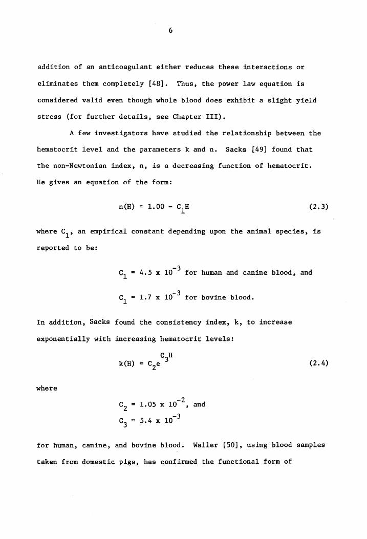
A few investigators have studied the relationship between the

hematocrit level and the parameters k and n. Sacks [49] found that

the non-Newtonian index, n, is a decreasing function of hematocrit.

He gives an equation of the form:

n(H) = 1.00 - C,H (2.3)

where Cy> an empirical constant depending upon the animal species, is

reported to be:

4.5.x 10°? for human and canine blood, and OQ i

=i1./7 x 107? for bovine blood. OQ |

In addition, Sacks found the consistency index, k, to increase

exponentially with increasing hematocrit levels:

C,H k(H) = Coe (2.4)

where

C, = 1.05 x 10°°, and

_ -3 C, = 5.4 x 10

for human, canine, and bovine blood. Waller [50], using blood samples

taken from domestic pigs, has confirmed the functional form of

equations (2.3) and (2.4). He obtained the following constants:

C, = 2.19 x 10>,

-2 C, = 2.95 x 10“, and

_ ~3 C, = 3.62 x 10~.

A search of the literature reveals that no studies have been

attempted to relate k and n to the chemical composition of the fluid,

or, at least no results have been published on this topic.

Some studies have been made relating the chemical composition

to viscosity. Rohrer [51,52] and Naegeli [53] report that the non-

protein constituents of serum play a minor role in determining the

viscosity of the fluid. The protein fractions have been found to

contribute in varying degrees. Rohrer [51,52] and Naegeli [53] found

that when equal amounts of globulin and albumin molecules are separate-

ly introduced into equal amounts of serum, it is the globulin sample

which shows a higher value of viscosity. Studies that have correlated

plasma viscosity with its protein fractions have repeatedly shown that

the larger the protein molecule and the more its shape differs from a

sphere, the larger the effect on viscosity [54-61]. Arranged in the

order of decreasing effects on viscosity at equal concentration, the

three major proteins are: fibrinogen, globulin, and albumin.

Lawrence [55] reports that although albumin, globulin, and fibrinogen

have concentration ratios of 4.0 : 2.5 : 0.3, respectively, their

contributions to viscosity increases are in the ratio 36 : 41 : 22.

Since the albumin solutions exhibit a lower viscosity than fibrinogen

and globulin solutions, Harkness [62] and Wells [63] suggest that

albumin may actually decrease the viscosity of plasma. In fact, the

viscosity of albumin solutions is lower than that of serum, and the

viscosity of fibrinogen and globulin solutions is higher than that of

serum. Merrill, et al. [41], show that a correlation exists between

viscosity and fibrinogen and the various types of globulins, but there

is no mention of albumin.

To the best of this author's knowledge, information relating

the plasma lipids to the viscosity of whole blood is not available in

the literature.

However, other investigators have studied numerous other

variables and their effect on the viscosity of blood. Isogai, et al.

[61], have studied the erythrocyte sedimentation rate (E.S.R.); Giombi

and Burnard [64] have looked at osmolality and pH; Gregersen, et al.

[43], have reported on the volume concentration and the size of the

red cells; and Hershko and Carmeli [65] have investigated packed cell

volume, hemoglobin content, and the red cell count.

C. Summary

It has been well documented that blood behaves as a combination

of a Bingham Plastic and a pseudoplastic fluid. When an anticoagulant

has been added, the Bingham Plastic behavior is no longer present to

any significant degree. Investigators have determined constitutive

equations for blood as a function of the shear rate and hematocrit

level. Studies have also been made relating plasma proteins to

viscosity, but this information has not been included in a constitutive

equation. Additionally, several investigators have considered the

E.S.R., osmolality, pH, hemoglobin content, size of the red cells,

and the red cell count.

CHAPTER IIL

The Present Problem

The present problem is to develop a practical and realistic

constitutive equation for whole human blood. When it is introduced

into the generalized momentum equations, this equation should be of a

form that they may be readily solved. Since the non-Newtonian behavior

of blood is primarily pseudoplastic, a general power law, such as

equation (2.2), will be examined. The Bingham Plastic behavior will

not be incorporated into this constitutive equation. This is justified

on the basis of two observations; first, the yield stress exhibited by

blood is extremely small and virtually constant; and, second, the power

law constitutive equation may be easily modified to allow for the

presence of a yield stress, i.e., it may be written as follows:

oH 2 t= ky + ty dynes/cm’. (3.1)

This merely shifts the ordinate values by an amount ty as shown in

figure 8.

The scope of this investigation is, first, to determine the

dependence of the consistency index, k, and the non-Newtonian index,

n, on the hematocrit level in an effort to verify equations (2.3) and

(2.4). The parameters k and n will also be examined as functions of

the plasma lipids and proteins. In each case the level of signifi-

cance of these equations will be determined.

10

CHAPTER IV

Method of Analysis

A. Materials

Over a period of five months beginning in March, 1974, exactly

200 human blood samples of 10 milliliters each were obtained from the

hematology laboratory of the Montgomery County Hospital. These human

blood samples, anticoagulated with EDTA, were mixed well by careful

shaking, and two 1.2 milliliter aliquots were drawn from each 10 milli-

liter test tube. Viscosity measurements at strain rates of 23.28,

46.56, 116.40, and 232.80 reciprocal seconds were recorded for each

aliquot, and the results at each shear rate were averaged. This

reduces the chance for an error due to incomplete mixing, inasmuch as

the pairs of viscosity values may be compared and if large discrepances

are noted, more viscosity measurements can be made,

A Wells-Brookfield Micro Cone and Plate Viscometer was used,

along with a Brookfield Model N recirculating constant temperature

water bath. The latter has an accuracy of + 0.01 degrees centigrade,

and the entire apparatus has been used with extreme accuracy by many

investigators. The most important feature of a cone and plate viscome-

ter is that it produces a constant strain rate in the fluid (see

appendix C for details). In addition, the optimum sample volume for

the viscometer is 1.2 milliliters, which is important when the fluid

being examined cannot be easily obtained in large quantities.

11

12

The chemical analysis (S.M.A. 10) of each blood sample was also

generously supplied by the Montgomery County Hospital. Total lipid

determinations were performed under the supervision of Dr. William

Gutstein at the New York Medical College in Valhalla, New York [73].

B. Variables

The dependence of the viscosity of blood upon the shear rate

and hematocrit level is well documented and will be included in the

constitutive model. The chemical parameters that will be investigated

include total lipids, albumin, and total protein minus albumin (TPMA).

TPMA is composed of fibrinogen and the globulin. These chemical

variables were chosen because they are composed of long chain

asymmetric molecules which exist in large numbers and interact more

than do symmetric particles. Thus, it is probable that they contri-

bute most to the rheologic properties of the fluid. Albumin, TPMA,

total lipid, hematocrit, and the strain rate will be treated as

independent variables, with the viscosity being considered dependent.

A multiple regression computer procedure will then be used to

determine the variables of greatest significance.

C. Statistical Analysis

Equation (2.2) is the basic functional form that will be

selected for developing the constitutive equation. Since the viscos-

ity of blood varies for different shear rates, we introduce a new

quantity called apparent viscosity (us) > which is defined as the

13

viscosity of the fluid at a given shear rate:

. w= t/Y poise. (4.1)

When equation (4.1) is substituted onto equation (2.2), an equation

relating the apparent viscosity to the shear rate results:

n-1 uo=k poise. (4.2) a

Equation (4.2) is nonlinear, making it extremely complicated from the

point of view of least squares regression analysis. Therefore, it is

more convenient to linearize the equation by taking logarithms to the

base e yielding:

logy, = log k + (n~1)1og.y- (4.3)

; 1 . 3, Ss Equation (4.3) is of the form: ,

Y = mX + b (4.4)

where

rd i dependent variable,

mo ui independent variable,

slope of the line, and 3 it

o it the Y intercept.

With respect to equation (4.3), these become:

log ou. = dependent variable,

log .¥ = independent variable,

14

(n-1) = slope of the curve, and

log .k = the intercept.

An equation which can be transformed in the manner just described is

called an intrinsically linear equation [66].

The parameters (n-1), log .k, and log shall be examined in

the regression analysis as functions of albumin, TPMA, total lipid,

hematocrit, their squares, their inverses, the squares of their

inverses, and all interaction terms (albumin x TPMA, albumin x Log .Y>

albumin x 1/hematocrit, and so forth). Log ua is the basic dependent

variable.

With respect to the inclusion of interaction terms such as

(L/hematocrit) x Log .Y and (1/hematocrit?) x logy» we note the

following:

Given a regression equation of the form:

log .u, = Cc, + C, ro (4.6)

if a variable such as

Yy = (l/hematocrit) x log .¥ (4.7)

is introduced, it suggests, for a constant shear rate, that an increase

in hematocrit will decrease the apparent viscosity. This is physically

unrealistic since the apparent viscosity of blood actually shows an

increase as the percentage by volume of erythrocytes increases. Terms

of the form (l/hematocrit) x log .Y and (1/hematocrit*) x log.y> there-

fore, are unrealistic and will not be allowed to appear in the model.

15

A maximum R-square improvement regression procedure, contained

in the Statistical Analysis System (S.A.S.) [67] of the VPI&SU 370 IBM

digital computer, was used to analyze the data. This procedure finds,

first, the "best" one variable model that produces the highest R-square

statistic (see appendix D). That is, of the independent variables

chosen for analysis, the program selects one and uses the linear least

squares method to determine an equation of the form (4.6). It then

computes an associated R-square statistic for this equation. Going

through this procedure separately for each independent variable, the

computer finally chooses the model with the largest R-square statistic

as the best one variable model.

To determine the best two variable model, the statistical

program now adds one of the remaining variables to the best one

variable model. The linear regression analysis is used to determine

an equation of the form:

log .u. = C, + Coy, + c.Y, (4.8)

and the associated R-square statistic for this equation is computed.

A different variable is then added to the best one variable model, and

again the R-square statistic is computed. This procedure is followed

for all remaining variables to determine which one, when added to Yq:

will produce the greatest increase in R-square.

At this point, it is realized that the Y, variable which pro- 1

duced the best one variable model may not necessarily be one of the

two which produces the best two variable model. Thus, the program

16

goes back to check each of the variables, both yy and Yo» in the model

it has just obtained. That is, it determines whether there will be a

further increase in the R-square value if either of the presently in-

cluded variables is replaced by one which was excluded. After all

possible comparisons are made, the combination of two variables which

produces the greatest increase in R-square over the previous two

variable model is isolated. The procedure continues cycling until no

increase in R-square is found. The result is the best two variable

model. Essentially, this procedure determines whether or not the

variable Y, in the best one variable model is also significant in the

best two variable model. For higher order models, the entire procedure

is repeated.

Since this study seeks a practical as well as realistic con-

stitutive equation, the best three variable model will be the highest

order model investigated. Furthermore, the model will be restricted

to the normal physiologic range of hematocrit, i.e., 35-50%.

CHAPTER V

RESULTS AND DISCUSSION

A. Preliminary Remarks

It has been well documented that the behavior of whole blood

is primarily pseudoplastic. That is, the viscosity decreases as the

shear rate increases. Therefore, it should not be too surprising to

find that the best one variable rheologic model shows the shear rate

to be the single most significant independent variable. This equation

is:

n-1 uae ky poise (5.1)

with

k = 0.134, and

n = 0.785 both constant.

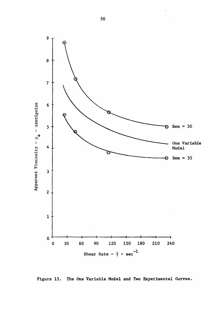
Equation (5.1) has an R-square value of 0.6187 and a mean square error

of 0.0218, so the fit of this equation to the data is not good enough.

Also, notice that n, the non-Newtonian index, is constant in this

model for all hematocrit levels and chemical compositions. Physically,

this is unrealistic, since the non-Newtonian properties of blood arise

from the interactions of red blood cells with each other and with the

long chain molecules present in the plasma. When the number of red

blood cells increase so does the non-Newtonian behavior. A plot of

equation (5.1) is shown in figure 13 along with two experimental

17

18

curves. It is not hard to see that an equation involving only the

shear rate is not a very good approximation of the true behavior of

blood. It would seem, therefore, that the hematocrit level should be

the next likely candidate for inclusion in the constitutive model.

B. Dependence on Hematocrit

The best two variable model (BTIVM) found by the multiple re-

gression procedure shows the shear rate and hematocrit level to be the

most significant independent variables. The equation has the same

form as equation (5.1) except that k and n now depend on the hematocrit

level as follows:

C, (Hematocrit) k = cje » and (5.2)

n= 1.0 - C, (Hematocrit), (5.3)

where

Cc, = 0.0148,

Co = 0.0512, and

Cy = 0.00499.

The R-square value for this model is 0.8789, while the mean square

error is 0.0069. Each coefficient, c,@ = 1,2,3), has a T value of

0.0001. The T value of the coefficient is a measure of the probability

that a variable is not statistically significant in the model. Thus

a T value of 0.0001 means that the probability of a variable being

Statistically significant is 99.992.

19

Equations (5.2) and (5.3) are in the same form as reported by

Sacks [49]. The differences appear in the coefficients C Co» and C 1’ 3”

as shown in Table I. Observe that the values for C, are of the same

order of magnitude. In fact, the coefficient from the best two variable

model is only 0.00049 larger than Sacks' value. Off hand, one might

attempt to attribute this small difference to experimental and statisti-

cal errors. However, it may be argued that the difference, though

small, is still meaningful because the very small mean square error

(a measure of the average distance each data point falls off the

regression line) and the very low T values indicate that the co-

efficients in this best two variable model are statistically quite

Significant. Thus the BIVM predicts a higher degree of non-Newtonian

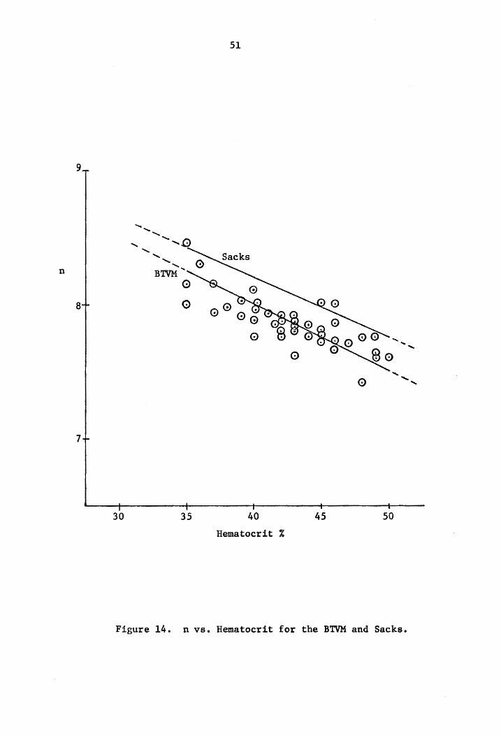
behavior than does the model reported by Sacks. Figure 14 shows

equation (5.3) with the Cy value from both Sacks' model and the BTIVM.

Clearly, the slope of the BIVM line is greater than the slope of

Sacks' line. Furthermore, by observing the experimental data which

are plotted on the same graph, we see that most of the points fall

much closer to the BTVM line. This tends to confirm that the

difference between Cy (Sacks) and C, (BTVM) is, in fact, significant

and not mainly due to experimental or statistical errors.

Table I shows that the two values of C, are again of the same 1

order of magnitude, but the values of C, differ by a full order of 2

magnitude. These coefficients appear in the equation for k. Sacks’

curve and the BTIVM curve for k are plotted in figure 15, and a

significant difference is immediately visible. Some experimental

20

data points are plotted to show the variance about the BIVM line.

The difference between the two lines is composed of a linear term and

a nonlinear term. The linear difference is the increase by 0.00436

of C, (BTVM) over Cc, (Sacks). The nonlinear difference arises from

the difference in the C, values, the C, (BIVM) value being 0.0458 2

larger. Thus, the BIVM consistently predicts a higher value of

apparent viscosity and this increase is nonlinear.

C. Dependence on Plasma Proteins

The first variable examined was total protein, hereafter

referred to as TP. TP is composed of fibrinogen, albumin, and

globulin. The normal physiologic ranges for these quantities are:

(1) fibrinogen, 0.2 to 0.6 gram/100 ml., (2) albumin, 3.5 to 5.5

gram/100 ml., and (3) globulin, 1.5 to 3.0 gram/100 ml. When TP was

added to the variables already under consideration in the BIVM, the

resulting best three variable model produced an R-square of 0.8836

which is an increase of only 0.00468 over the BIVM. This implies

that TP does not have much of an effect on the viscosity of blood,

which is an unexpected finding when one considers that the plasma

proteins are very long chain asymmetric molecules which interact

strongly with each other and with the red blood cells.

Pursuing this point further, the author discovered articles

by Harkness [62] and Wells [63], in which it was reported that saline

solutions of albumin have significantly lower viscosities than do

equivalent solutions of globulin. Therefore, it would seem likely

21

that, since albumin and globulin are two of the primary constituents

of total protein, they could have cancelling effects when introduced

as a single variable. Thus, the single variable, total protein, was

separated into albumin and total protein minus albumin (or TPMA).

TPMA is composed of globulin and fibrinogen, these two being combined

into a single variable for two reasons: (1) globulin saline solutions

and fibrinogen saline solutions each have higher viscosities than

albumin solutions; and (2) no specific information concerning the

fibrinogen concentration was available for the blood samples used in

this study.

A three variable model including albumin was not generated by

the regression analysis, but there was a model developed containing

TPMA. Thus, it may be inferred that albumin does not affect viscosity

at the same level as does TPMA. This can be partially explained by

noting that albumin has a molecular weight of 66,000 and an axial

length-width ratio of 3 : 1, while TPMA is composed of molecules

having molecular weights ranging from 35,000 to 1,000,000 with axial

length-width ratios of 12 : 1 and greater. Studies [54-61] have shown

that the larger the molecule and the more its shape differs from a

sphere, the greater the effect on viscosity. Thus, it is not

surprising to find that TPMA enters into the constitutive model before

albumin, although it is not immediately obvious why this finding should

be masked when albumin is lumped with the other proteins in the model.

Perhaps the observation that rouleaux formations (aggregations of red

blood cells), caused by fibrinogen and other fibrous proteins, were

22

found to be dispersed by serum albumin could play a role in explaining

the latter observation.

The best three variable model is exactly the one which includes

TPMA and this model has the form:

n-1

ue ky poise, (5.4)

where

C., (Hematocrit) + C, aa)

k = c,e Hematocrit , and (5.5)

n= 1.0 - C, (Hematocrit). (5.6)

The coefficients in equations (5.5) and (5.6) have the values:

Cy = 0.00797,

C. = 0.0608,

C, = 0.00499, and

C, = 145.85.

The R-square for this model is 0.9049, a significant increase of

0.0259 over the BIVM. The mean square error of 0.00546 is over 27%

less than that for the BIVM and the T values for the coefficients are

0.0001 each. Thus, introducing TPMA into the model produces a

statistically significant increase in fitting the data.

Table II shows a comparison of the BIVM and the best three

variable model. Note that C35 the constant in the equation for n,

is identical for both models. Therefore, this study shows that

hematocrit is primarily responsible for the non-Newtonian index of

blood and that the plasma lipids and proteins have little or no affect

on this index, n.

Also, observe in Table II, that the corresponding values of C 1

and C, are approximately of the same order of magnitude. The

difference, therefore, between the two models arises primarily from

the term in brackets, i.e.,

P TPMA ) C, (

Hematocrit”

e

The range of values for this term at various hematocrit levels is

shown in Table III for the two extreme values of TPMA considered in

this study. Note that the value of K decreases with increasing

hematocrit at constant values of TPMA, and vice-versa. Physically,

this is reasonable, since when hematocrit, which has a first order

effect on viscosity, is low, one would expect second order effects,

such as the chemistry of the fluid, to become more important. This

is exactly the behavior which equation (5.5) predicts. Mathematically,

the limiting case is for an infinite hematocrit level, at which point

X is equal to unity and thus has no effect on viscosity.

A comparison of the consistency index equations ((5.2) and

(5.5)) for the BIVM and the best three variable model can be seen in

figure 16. The highest and lowest values of TPMA used in this study

are plotted along with the consistency index equation from the BIVM.

The curves corresponding to other values of TPMA lie between the two

extremes shown. Note that the best three variable model curve with

24

TPMA equal to 1.5 falls below the BIVM, while the curve for TPMA equal

to 4.2 lies above the BIVM curve.

Similar behavior is shown in figures 17 through 22, which are

plots of apparent viscosity versus shear rate for various hematocrit

and TPMA levels. Several important results may be discerned from

these figures.

First, it can be seen that TPMA has a significant effect on

viscosity, a fact not revealed in the BIVM. Compared with the BTIVM,

the best three variable model shows that blood with relatively low

levels of TPMA has a correspondingly lower apparent viscosity and the

latter increases with TPMA. Thus, the best three variable model pre-

dicts either higher or lower fluid shear stresses (depending on the

TPMA concentration) than does the BIVM.

Second, since the fluid viscosity is greatly dependent on

hematocrit, note from figures 17-22 that the best three variable model

curves converge around the BIVM as the hematocrit level progressively

increases. This can be observed especially well at the lower shear

rate ranges.

The increase in non-Newtonian behavior as the hematocrit

level goes up, is also visible in figures 17-22. This behavior is

illustrated even more clearly in figure 23, where curves of the best

three variable model at various hematocrit levels are plotted with

TPMA held constant.

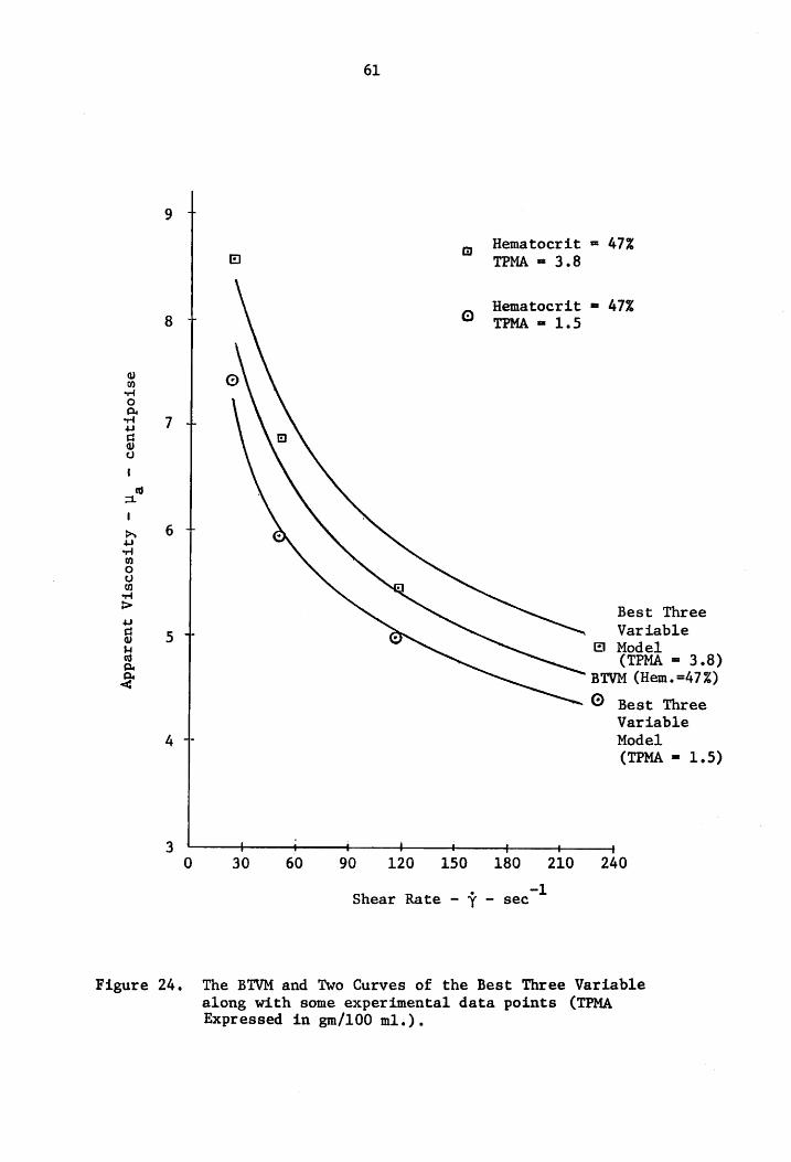
Figure 24 shows a plot of the best three variable model for

a low (1.5) and a high (3.8) TPMA level, with hematocrit held constant.

25

“Experimental data points corresponding to these TPMA levels are also

shown, as is a plot of the BIVM. This figure illustrates clearly that

it is the high and low values of TPMA that produce a significant change

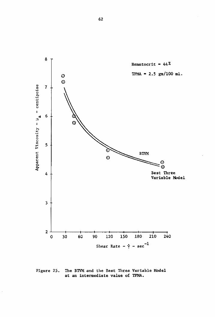
from the BIVM. For example, figure 25 shows that for an intermediate

value of TPMA (2.5) there is not much difference between the two

modeis. Therefore, it may be concluded that if one is interested in

examining fluid behavior at moderate levels of TPMA (2.5 + 0.2)

either a two or three variable model would be appropriate, but if a

wider range of TPMA is to be investigated, then the best three variable

model should be chosen.

D. Dependence on Plasma Lipids

On the basis of an intensive literature search, this author

could find no work relating the plasma lipids to the viscosity of

whole blood. The only references which dealt with lipids were those

of Rohrer [51,52] and Naegeli [53] which were published in 1916 and

1923 respectively. These investigators reported that the non-protein

constituents of serum play a minor role in determining the viscosity

of the fluid. The results of the present study tend to confirm this

finding, at least for the case of the plasma lipids.

The only reasonable model which includes total lipids has an

R-square value of 0.8805. It has the form of equation (5.1) where

C, (Hematocrit) + C total lipid, 2 5

albumin k = C.e ,» and (5.7)

26

n= 1.0 - C., (Hematocrit) (5.8)

with the constants given as follows:

Cc, = 0.0434,

Cc, = 0.00059,

C, = 0.0051, and

C. = 0.900.

The T value for each of the above coefficients is 0.0001 and the mean

square error is 0.00714, so statistically this model is significant.

However the R-square increase over the BIVM is 0.00149, only a 0.172%

increase, and is actually 0.0244 less than the best three variable

model discussed previously in section C. Consequently, this study

confirms that the plasma lipids probably play a minor role in

affecting the viscosity of blood.

CHAPTER VI

Summary and Conclusions

A. Constitutive Equations Developed

Three rheologic equations, from a one variable model to a

three variable model, were developed in this study. As the number

of variables increased, so did the statistical fit to the experi-

mental data. The equations for k and n were developed from a relation

of the form

n-lL

w= ky poise. (6.1)

By definition, a constitutive equation relates the stress to the rate

of strain in a fluid. In this study a power-law functional form was

assumed, i.e.,

" 2 t= kY dynes/cm’. (6.2)

where

t = the shear stress,

Y = the shear rate,

k = the consistency index, and

n = the non-Newtonian index.

The best one variable model led to the following results:

k = 0.134 = constant, (6.3)

n = 0.785 = constant, (6.4)

R~square = 0.6187,

27

28

mean square error = 0.0218, and

T = 0.0001.

The best two variable model yielded:

C, (Hematocrit)

k = ce » and (6.5)

n=1.0- C. (Hematocrit), (6.6)

where

C, = 0.0148,

C, = 0.0512, and

C, = 0.00499.

The R-square value for this model is 0.8789; the mean square error

equals 0.0069; and the T values are 0.0001.

The best three variable model has the form

TPMA ) C, (Hematocrit) + C, ¢ 9

k= Ce Hematocrit , and (6.7)

n= 1.0 - C, (Hematocrit), (6.8)

where

oO I = 0.00797,

OQ i = 0.0608,

© I = 0.00499, and

145.85. OQ Q

29

The R-square value is 0.9049, the mean square error is 0.00546, and the

T values equal 0.0001.

In each of the rheologic models developed, the variables /Y,

hematocrit, TPMA, albumin, and total lipid were considered to be

independent variables. That is, it was assumed that a change in one

variable would not produce a change in any of the others. In reality,

blood in the cardiovascular system of man and animals is constantly

changing in chemical composition and shear rate--the two having a non-

linear interrelationship. Additionally, the various chemical con-

stituents are dependent on each other. These complexities tend to

invalidate the assumption of the independence of chemical variables.

However, for a first order effect of chemical composition on viscosity,

the assumption of independence of chemical variables is reasonable.

B. Results Summarized and Conclusions

An equation including only the shear rate was found to be

lacking any real degree of significance. When hematocrit was added

as a variable, the R-square increased from just 62% to almost 882.

Of the chemical variables studied, the least significant, as far as

effects on viscosity is concerned, was the plasma lipids. Fibrinogen

and globulin, in the form of TPMA, had a much greater effect on

viscosity than did albumin. The best three variable model, which

includes TPMA, increased the R-square from 88% to nearly 91%--a

significant increase,

30

On a microstructural level, there is much to be done, but for

a first order approximation of the effects of plasma chemistry on

whole blood viscosity, this thesis offers a reasonable constitutive

equation.

C. Direction of Future Studies

Information about the fibrinogen concentration would be

desirable in order to determine which of the two variables comprising

TPMA has the most effect'on viscosity. Moreover, in a future study

the chylomicron count might be examined. Chylomicrons are globules

of emulsified fats and are large enough to be seen with a light

microscope. In addition, the chylomicron count is expressed in

volume percent, which, dimensionally, is more compatible with hemato-

crit than is gram percent (gm/100m1). Many other variables should

also be investigated. These include the various subgroups of the

globulins and albumin. Perhaps even the shape of the hematocytes

could be related to the viscosity of blood.

10.

li.

12.

13.

14.

REFERENCES

Galen, "On the Natural Faculties," in: Hutchins, R. M. (Editor in Chief), Great Books of the Western World, Volume 10, Encyclopaedia Britannica, Inc., Chicago.

Leake, C. D., "The Historical Development of Cardiovascular Physiology," in: Hamilton, W. F., (Section Editor) and Dow, P. (Executive Editor), Handbook of Physiology, Section 2: Circula- tion, Volume II, American Physiological Society, Washington, D.C., 1963, pages 11-22.

Hess, W., Vischr. Naturf. Ges. Zurich, Vol. 51, page 236, 1906.

Fahraeus, R., Cause of the Decreased Stability of Suspensions of Blood Corpuscles during Pregnancy, Biochem. Z. Vol. 89, pages 355-364, 1918.

Fahraeus, R., The Suspension-stability of the Blood, Acta Med. Scand., Vol. 55, pages 1-228, 1921.

Fahraeus, R., Suspension Stability of the Blood, Physiol. Rev., Vol. 9, page 241, 1929.

Holker, J., The Viscosity of Syphilitic Serum, J. Path. Bact., pages 413-418, 1921.

Schwalm, H., Viscosimetric Im Blut, Plasma, Serus und Anderen Korperflussigkeiten Mit Neuer Methode, Arch. Gynaek., Vol. 172, pages 288-328, 1941-42.

Ley, R., Ueber Die Sedimentierungsgeschwindigkeit Der Roten Blutkorperchen, Z. Ges. Exp. Med., Vol. 26, pages 59-68, 1922.

Petschaher, L., Specific Viscosity of Serum Protein, Z. Ges.

Exp. Med., Vol. 41, pages 142-156, 1924.

Petschaher, L., Z. Ges. Exp. Med., Vol. 41, page 331, 1924.

Hertwig, H., Beitr. Z. Klin. D. Tubercl., Vol. 70, page 715, 1928.

Chopre, R. N. and Choudhury, S. G., Studies in Physical Properties of Different Blood Serum Viscosity, Indian J. Med. Res., Vol. 16, pages 939-945, 1929.

Bircher, M. E., Clinical Diagnosis by Viscosimetry of the Blood and the Serum with Special Reference to the Viscosimeter of W. R. Hess, J. Lab. Clin. Med., Vol. 7, pages 134-147, 1922.

31

15.

16.

17.

18.

19.

20.

21.

22.

23.

24.

25.

26.

27.

28,

32

Bircher, M. E., The Value of the Refracto-viscosimetric Prop-

erties of the Blood Serum in Cancer, J. Lab. Clin. Med., Vol. 7,

pages 660-664, 1922.

Bircher, M. E., The Value of the Refracto-viscosimetric Prop-

erties of the Blood Serum in Cases of Tuberculosis, J. Lab.

Clin. Med., Vol. 7, pages 733-735, 1922.

Bircher, M. E. and McFarland, A. R., Globulin Content of Blood

Serum in Syphilis, Arch. Derm. Syph., Vol. 5, pages 215-233,

1922.

T'ang, B. H. Y. and Wang, S. H., Chinese Med. J., Vol. 57, page

546, 1940.

Whittington, R. B., Blood Sedimentation; A Study in Haemo-

mechanics, Proc. R. Soc. (B), Vol. 131, pages 183-190, 1942.

Miller, A. K. and Whittington, R. B., Plasma-Viscosity in

Pulmonary Tuberculosis, Lancet, Vol. 2, pages 510-511.

Houston, J., Harkness, J., and Whittington, R. B., Br. Med. J., Vol. 2, page 741, 1945.

Cowan, I. C. and Harkness, J., The Plasma Viscosity in Rheumatic Diseases, Br. Med. J., Vol. 2, pages 686-688, 1947.

Harkness, J., Effects of Sulphonamides on Serum Protein, Plasma Viscosity, and Erythrocyte-Sedimentation Rate, Lancet, Vol. 1, pages 298-299, 1950.

Womersley, J. R., Oscillatory Motion of a viscous Liquid in a Thin-Walled Elastic Tube. I. The Linear Approximation for Long

Waves. Ser. 7, Vol. 46, No. 373, Feb. 1955.

Bodley, W. E., The Non-Linearities of Arterial Blood Flow. Phys. Med. Biol., Vol. 16, No. 4, pg. 663-672, 1971.

Landowne, M., Pulse Wave Velocity as an Index of Arterial Elastic

Characteristics, in: Remington, J. W., Tissue Elasticity,

American Physiology Society, Washington, D. C.

Schneck, D. J., Pulsatile Blood Flow in a Diverging Circular Channel, Ph.D. Thesis, Jan. 1973, Case Western Reserve University, Cleveland, Ohio.

Bergin, J. M., and Ostrach, S., On Impulsive Periodic Motion and Blood Flow, Case Western Reserve University, School of Engineering, Division of Fluid, Thermal and Aerospace Sciences,

FTAS/TR-69-40, April, 1960.

29.

30.

31.

32.

33.

34.

35.

36.

37.

38.

39.

33

Spillane, M. W. and Ostrach, S., Entrance Flow in a Converging Elastic Tube, Case Western Reserve University, School of Engineering, Division of Fluid, Thermal and Aerospace Sciences, FTAS/TR-67-19, June, 1967.

Spillane, M. W. and Ostrach, S. Unsteady Flows in Tapering Elastic Vessels, Case Western Reserve University, School of Engineering, Division of Fluid, Thermal and Aerospace Sciences, FTAS/TR-69-46, June 1970.

Kuchar, N. R. and Ostrach, S., Unsteady Entrance Flows in Elastic Tubes with Application to the Vascular System, Case Western Reserve University, School of Engineering, Division of Fluid, Thermal and Aerospace Sciences, FTAS/TR-67-25, November, 1967.

Wu, H. and Ostrach, S. Wave Reflection in Flexible Tubes, Case Western Reserve University, School of Engineering, Division of Fluid, Thermal and Aerospace Sciences, FTAS/TR-69-44, June 1969.

Jones, E., Chang, I-Dee, Anliker, M. Effects on Viscosity and External Constraints on Wave Transmission in Blood Vessels,

Stanford University, Depargment of Aeronautics and Astronautics, SUDAAR No. 344, May 1968.

Fry, D. L. and Greenfield, J. C., The Mathematical Approach to Hemodynamics, with Particular Reference to Womersley's Theory,

in: Attinger, E. 0. (Editor), Pulsatile Blood Flow, New York, McGraw-Hill Book Company, The Blakinston Division, 1964.

Wilkinson, W. L., Non-Newtonian Fluids, New York, Pergamon

Press, 1960.

Merrill, E. W., Gilliland, E. R., Margetts, W. G., Hatch, F. T.,

Rheology of Human Blood and Hyperlipemia, J. Applied Phys., Vol. 19, No. 3, pages 493-496, 1964.

Cokelet, G. R., Merrill, E. W., Gilliland, E. R., Shin, H., Britten, A., and Wells, R,. E., The Rheology of Human Blood-- Measurement Near and at Zero Rate of Shear, Trans. Soc. Rheol., Vol. 7, pages 303-317, 1963.

Charm, S. and Kurland, G. S., Viscometry of Human Blood for Shear Rates of 0-100,000 sec, Nature (London), Vol. 206, pages 617-618, 1965.

Casson, N., A Flow Equation for Pegment-oil Suspensions of the Printing Ink Type, in: Mill, C. C. (Editor), Rheology of

Disperse Systems, Pergamon Press, London, pages 84-102, 1959.

40.

41.

42.

43.

44,

45.

46.

47.

48.

49,

50.

Merrill, E. W., Gilliland, E. R., Cokelet, G., Shin, H., Britten, A. and Wells, R. E., Rheology of Human Blood, Near and at Zero Flow--Effects of Temperature and Hematocrit Level, Biophysics J., Vol. 3, pages 199-213.

Merrill, E. W., Margetts, W. G., Cokelet, G. R., Britten, A., Salzman, E. W., Pennell, R. B., and Melin, M., Influence of Plasma Proteins on the Rheology of Human Blood, in: Copely, A. L. (Editor) Proc. Fourth Int. Congr. on Rheol. 4, Symp. on Biorheol., Interscience, New York, pages 601-611, 1965.

Chien, S., Usami, S., Taylor, H. M., Lundberg, J. L., Gregersen, M. I., Effects of Hematocrit and Plasma Proteins on Human Blood

Rheology at Low Shear Rates. J. Applied Physiol., Vol. 21, pages 81-87.

Gregerson, M, I., Peric, B., Chien, S., Sinclair, D., Chang, C. and Taylor, H. Viscosity of Blood at Low Shear Rates in:

Copely, A. L. (Editor), Proc, Fourth Int. Congr. on Rheol. 4, Symp. on Biorheol., Interscience, New York, pages 613-628, 1965.

Charms, S. and Kurland, G. S., Tube Flow Behavior and Shear Stress/Shear Rate Characteristics of Canine Blood, Am. J. Physiol., Vol. 203, pages 417-421, 1962.

Bugliarello, G. and Hayden, J. W. Detailed Characteristics of the Flow of Blood in Vitro, Trans. Soc. Rheol., Vol. 7, pages 209- 230, 1963.

Bugliarello, G., Kapur, C. and Hsiao, G., The Profile Viscosity and Other Characteristics of Blood Flow in a Non-Uniform Shear Field, in: Copely, A. L. (editor) Proc. Fourth Int. Congr. on Rheol. 4, Symp. on Biorheol., Interscience, New York, pages 351-

370, 1965.

Barras, J. P., Blood Rheology-General Review, Bibl. Haemat., Vol. 33, pages 277-297, 1969.

Cokelet, G. L., The Rheology of Human Blood, Ph.D. Thesis, Department of Chemical Engineering, Massachusetts Institute of Technology, January, 1963.

Sacks, A. H., Raman, K. R., Burnell, J. A., and Tickner, E. G., Auscultatory Versus Direct Pressure Measurements for Newtonian

Fluids and for Blood in Simulated Arteries, VIDYA Report #119, December 30, 1963.

Waller, M. D., Personal Communication.

ol.

32.

53.

54.

55.

56.

57.

58.

59.

60.

61.

62.

63.

64,

35

Rohrer, H., Dutsch. Arch. Klin. Med., Vol. 121, pages 221, 1916.

Rohrer, H., Schweiz. Med. Wschr., Vol. 22, page 555, 1917.

Naegeli, O. Blutkrankheiten und Blutdiagnostik, 4th edition, Verlag von Julius Springer, Berlin, 1923.

Harkness, J. On the Viscosity of Human Blood Plasma and Serum in Health and Disease, Thesis for Degree of Doctor of Medicine, University of Glasgow, 1952.

Lawrence, J. S., Assessment of the Activity of Disease, Lewis, H. K., London, 1961.

Harkness, Jr. and Whittington, R.-B., Variations of Human Plasma

and Serum Viscosities with Their Protein Content, Bibl. Anat.,

Vol. 9, pages 226-231, 1967.

Pavey, R. A., The Measurement of Viscosity of Human Blood Plasma

and Serum, Thesis for Fellowship of Institute of Medical Laboratory Technicians, 1968.

Somer, T., Viscosity of Blood, Plasma, and Serum in Dys. and Paraproteinemias, Acta. Med. Scand. Suppl., Vol. 180, Suppl. 456, pages 1-97, 1966.

Eastham, R. D., The Serum Viscosity and the Serum Proteins, J.

Clin. Path., Vol. 7, page 66, 1954.

Hess, E. L. and Cobure, A. J., Intrinsic Viscosity of Mixed Protein Systems Including Studies of Plasma and Serun,

J. Gen. Physiol., Vol. 33, pages 511-523, 1950.

Isogai, Y., Ichiba, A. A. and Nagaoka, H., On the Interrelation Between Blood Viscosity and the Erythrocyte Sedimentation Rate. Biorheology, Vol. 6, page 245, 1970.

Harkness, J. The Viscosity of Human Blood Plasma, Biorheology, Vol. 8, pages 171-193, 1971,

Wells, R. E. The Effects of Plasma Proteins Upon the Rheology of Blood in the Microcirculation, in: Copely, A. L. Proc. Fourth Int. Congr. on Rheology 4, Symp. on Biorheol., Inter- science, New York, pages 351-370, 1965.

Giombi, A. and Burnard, E. D. "Rheology of Human Foetal Blood with Reference to Haematocrit, Plasma Viscosity, Osmolality, and pH., Biorheology, Vol. 6, pages 315-328, 1970.

65.

66,

67.

68.

69.

70.

71.

72.

73.

36

Hershko, C. and Carmeli, D. The Effect of Packed Cell Volume, Hemoglobin Content and Red Cell Count on Whole Blood Viscosity, Acta. Haemat., Vol. 44, pages 142-154, 1970.

Draper, N, R. and Smith, H., Applied Regression Analysis, John Wiley and Sons, Inc., New York, page 264, 1966.

Service, J. A User's Guide to the Statistical Analysis System, Student Supply Stores, North Carolina State University, Raleigh,

North Carolina, August 1972.

Wilkinson, W. L., Non-Newtonian Fluids, Pergamon Press, New York, 1960.

Christensen, R. M. Theory of Viscoelasticity, Academic Press, New York, 1971.

Astarita, G. and Marrucci, G., Principles of Non-Newtontian Fluid Mechanics, McGraw-Hill Book Company, England, 1974.

Fung, ¥. C. A First Course in Continuum Mechanics, Prentice-Hall Inc., New Jersey, page 36, 1969,

Tullis, J. L. (Editor), Blood Cells and Plasma Proteins, New York, N. Y., 1953.

Zollner, N. and Kirsch, K., Total Lipids, Z. Ges, Exp. Med., Vol. 135, page 545, 1962.

FIGURES

37

38

y

h

moving with a velocity uy, ——_———_—__—_—_——_—>

= Yo 4 Yo "0

\\\\\\)

Stationary

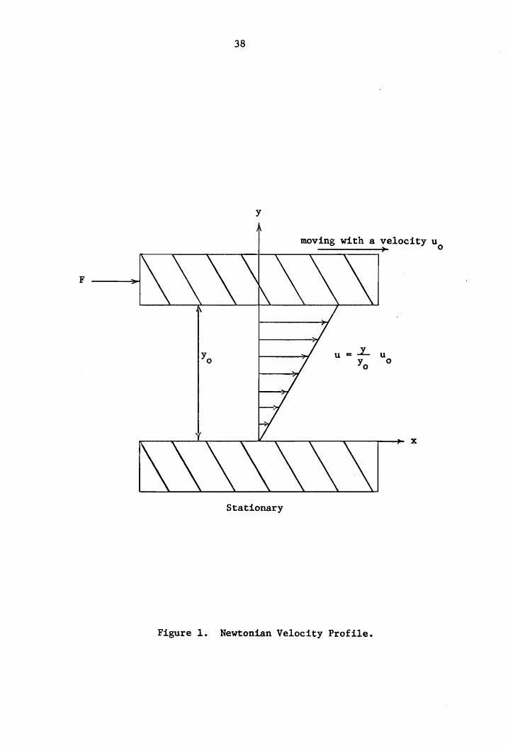
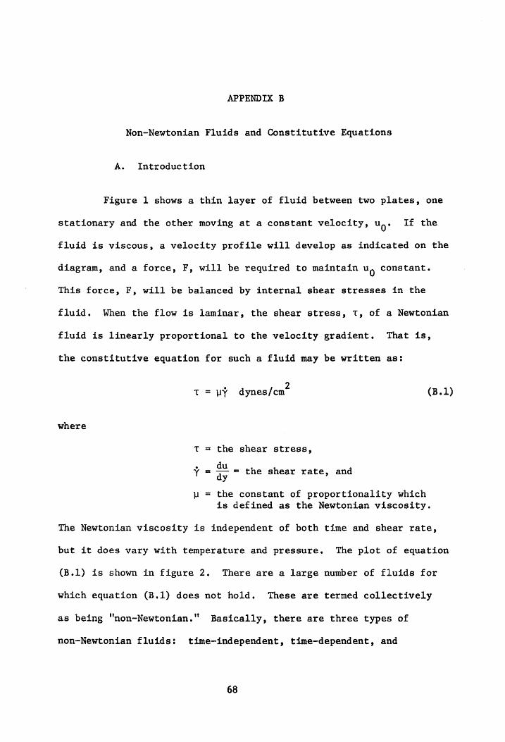
Figure 1. Newtonian Velocity Profile.

Shear

Stress

- T

39

Shear Rate 7

Figure 2. Types of non-Newtonian Fluids.

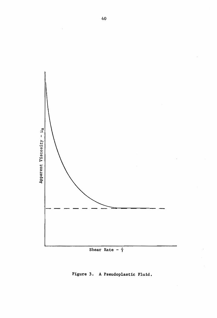
Apparent

Viscosity

- ug

40

Shear Rate - ¥

Figure 3. A Pseudoplastic Fluid.

Apparent

Viscosity

- Ha

41

start after standing for a long time

shear rate

increasing

Time

Figure 4. Behavior of a Time Dependent Fluid.

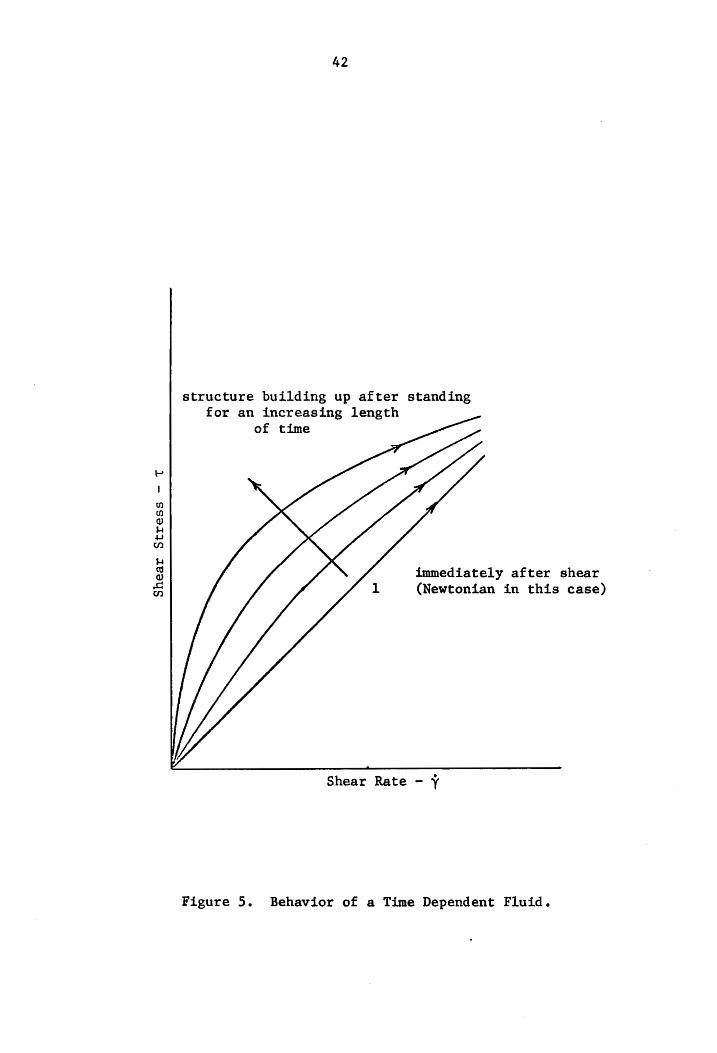
Shear

Stress

- T

42

structure building up after standing for an increasing length

of time

immediately after shear 1 (Newtonian in this case)

Shear Rate - ¥

Figure 5. Behavior of a Time Dependent Fluid.

Shear

Stress

- T

oe 43

pseudoplastic

Newtonian

Shear Rate - ¥

Figure 6. Hysteresis Loops.

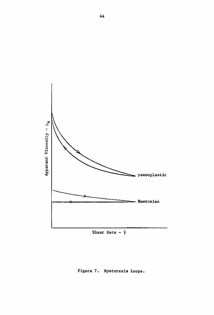
Apparent

Viscosity

- Ha

44

pseuoplastic

oe newtontan —

Shear Rate - ¥

Figure 7. Hysteresis Loops.

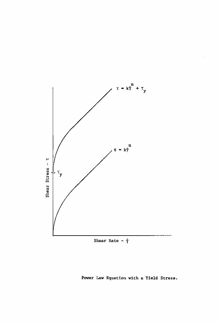
Shear

Stress

- T

k n T= + T

v y

t= ky

Shear Rate - ¥

Power Law Equation with a Yield Stress.

*uoTIeANSTJUuo)

suoy

azetd

VAN ANANNANANANAN

ANNAN AANANANANANANNN

I< aP

a 5

> 1

y vezus= dO

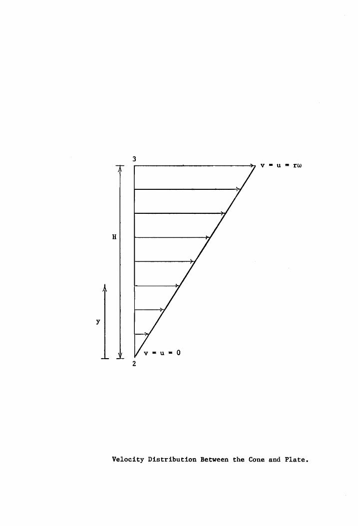
Velocity Distribution Between the Cone and Plate.

elemental

ring

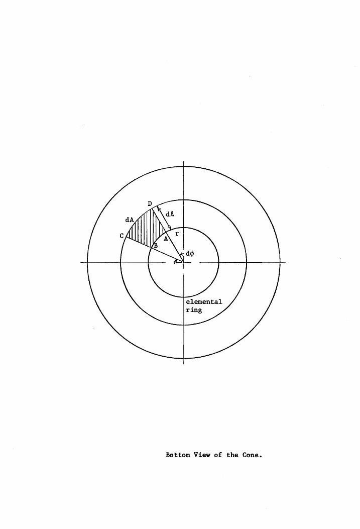
Bottom View of the Cone.

49

true equation

regression equation Figure 12. A True Equation and a Regression Equation

50

9 —

8+

ir

a 67 of

oO A, aa 4

a

, oO 5 5 Hem = 50

|

ow =i

' One Variable

» 44 Model nar cf]

9 Hem = 35 n rd >

v 37 ¢ o +S 3)

A <j 21

1+

0 t + t ' + + 4 —t

0 30 60 90 120 150 180 210 240

Shear Rate - Y - sec +

Figure 13. The One Variable Model and Two Experimental Curves.

51

1 “Fy t + t 30 35 40 45 50

Hematocrit 7%

Figure 14. n vs. Hematocrit for the BTIVM and Sacks.

52

16+

144

k x

107

107 6 i t | {

35 40 45 50

Hematocrit %

Figure 15. Comparison of k vs. Hematocrit for the BIVM and Sacks.

21 +

19 T

15+

kx

107

11 J

Figure 16.

53

i

T

35 40 45 50 Hematocrit Z

Three Variable

Model

TPMA = 4.2

BIVM

Three Variable

Model

TPMA = 1.5

Comparison of k vs. Hematocrit for the BIVM and the Best Three Variable Model.

’ T

Hematocrit = 35%

n = 0.8254

6 i

g 5 7 a o Ay

oa iw

¢ wo Oo

ai TPMA=4.0 k-10.81 ! > ay TPMA=3.5 k=10.19 “A g TPMA=3.0 k= 9.60 Y o

io TPMA=2.5 k= 9.04

u TPMA=2.0 k= 8.52

Y BIVM k=8.94 TPMA=1.5 k= 8.03 co 3+ a <q

2 + — + { ‘ —+ + —+

30 60 90 120) 6150 180 210 240

Shear Rate - Y - sec.

Figure 17. The Best Two and Three Variable Models at a Hematocrit Level of 35% (TPMA Expressed in gm/100 m1.)

55

k=12.08

k=11.48

k=10.92

k=10.38

k= 9.87

k= 9.38

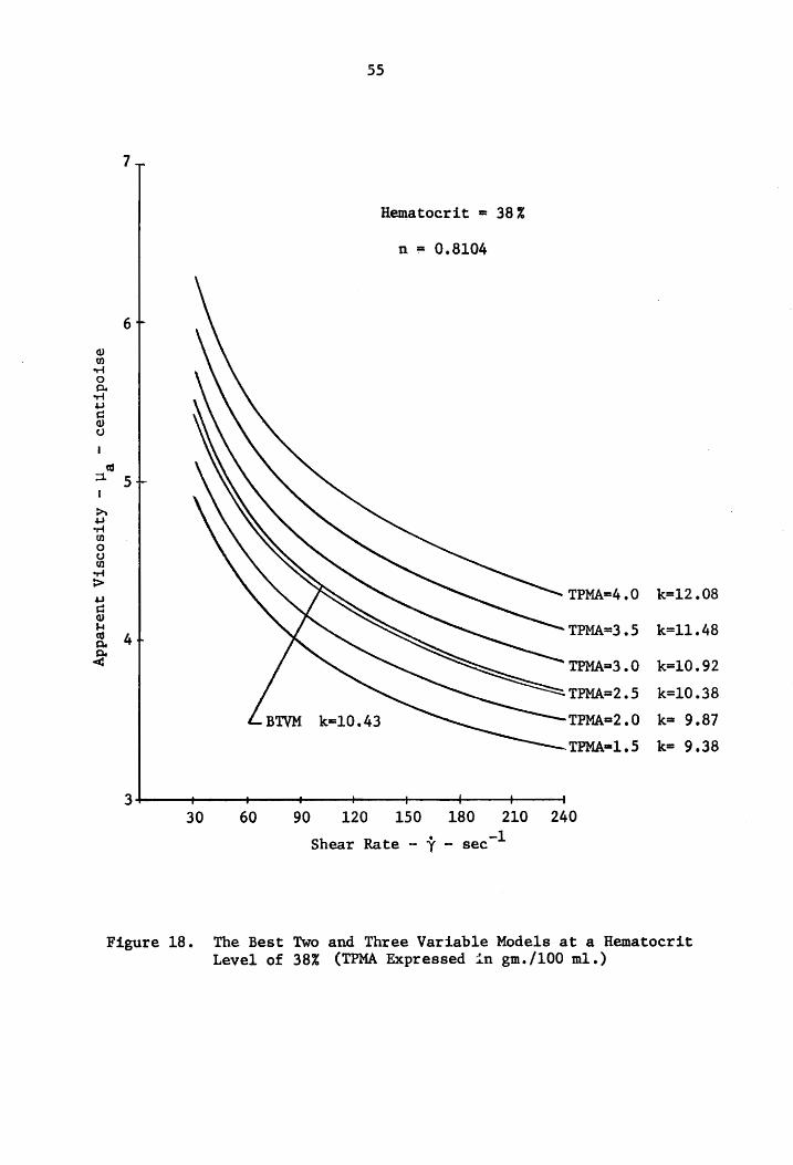
7+

Hematocrit = 38%

n = 0,8104

6 -

v on a o Au a

Ww

a a uo i 0

a 5+

i > 43 “4 Yn oO Y a aa >

a Ss at TPMA=3 .5 a < TPMA=3 .0

TPMA=2.5

BIVM k=10.43 TPMA=2 .0

TPMA=1.5

3 t + + ' 4 + 1 30 60 90 120 150 180 210 240

Shear Rate - Y - sec 2

Figure 18. The Best Two and Three Variable Models at a Hematocrit Level of 38% (TPMA Expressed in gm./100 ml.)

56

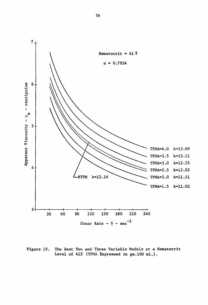
k=13.69

k=13.11

k=12.55

k=12.02

k=11.51

k=11.02

7a

Hematocrit = 414

n = 0,7954

y 6+ a= ° A, f 4

a v I «

a i

B 5+ rf 1] ° YO n rf >

@ 4 TPMA=3.5 A. 7 , TPMA=3 .0

1 TPMA=2.5 —BIVM k=12.16 TPMA=2 .0

TPMA=1.5

3 t — | ' t ' ' 30 60 90 120 150 180 210 £240

Shear Rate = 7 - sec.

Figure 19. The Best Two and Three Variable Models at a Hematocrit

Level of 41% (TPMA Expressed in gm.100 ml.).

57

8 1

Hematocrit = 442

n = 0.7804

27 4 orf oO A. A 4J

a @ YO

I

os st

1

P 6+ +d

uv

O vy on

aa >

43

q oO u

& < 5 ae

TPMA=4.0

TPMA=3.5

TPMA=3.0 BIVM k=14.18

TPMA=2.5

4 a TPMA=2.0

TPMA=1.5 i 4 i a a |

30 60 90 120 150 180 210 240

Shear Rate - ¥ - sec

k=15.70

k=15.12

k=14 .56

k=14.02

k=13.50

k#13.01

Figure 20. The Best Two and Three Variable Models at a Hematocrit Level of 44%. (TPMA Expressed in gm./100 ml.).

58

8 +

Hematocrit = 472%

n = 0.7655

o 2 t 417 A di 43

c o vO

\

os a

i

PP 4 6} oO oO n

ot >

4J

5 44 w

a a

5 TPMA=4.0 k=18.16

TPMA=3.5 k=17.57

BIVM k=16.54 TPMA=3.0 k=17.00

TPMA=2.5 k=16.44

TPMA=2.0 k=15.91

TPMA#1.5 k=15.39

4 + + + + + +

30 60 90 120 150 180 210 240

Shear Rate - 7 - sec.

Figure 21. The Best Two and Three Variable Models at a Hematocrit

Level of 47% (TPMA Expressed in gm./100 ml.).

39

k=21.13

k=20.53

k=19.94

k=19.36

k=18 .81

k=18.27

+ Hematocrit = 50%

n = 0.7505

o 87 fl ° a

“el $3

a o oO

i 3

a '

o7 + er an O° og Le) ef > 4

3 H w

a: <

6+

TPMA=4 .0

em 19.29 TPMA=3 .5

BIVM kel. TPMA=3 .0 27 TPMA=2.5

TPMA=2 .0

TPMA=1.5

30 60 90 120 150 180 210 249

Shear Rate - Y - sec.

Figure 22. The Best Two and Three Variable Models at a Hematocrit Level of 50% (TPMA Expressed in gm./100 ml.).

60

8 +

7.

w on

orf ° A

par 45

G go 7 \

ws a

i > 43

par wn

° 257

orf >

a k=18 .27 @ u a: & k=15.39

4+ k=13.01

_k=11.02

k= 9.38

k= 8.03 3 ' + + —t + {———+

30 60 90 120 150 180 210 240

Shear Rate - ¥ - sec

Figure 23. The Best Three Variable Model at a TPMA Level of

1.5 gm/100 ml.

n=0.7505

n=0.7655

n=0.7804

n=0.7954

n=0.8104

n=0.8254

61

9 =

a Hematocrit = 47% E TPMA = 3.8

© Hematocrit = 47%

8 + TPMA = 1.5

wo n rd oO

a vw 7 + rat vo v

{

0 1.

1

> 67 4J

rar a oO

a ord

= Best Three

a 5 + Variable

M4 El Model a (TPMA = 3.8)

a BTVM (Hem.=47%) © Best Three

Variable

ar Model

(TPMA = 1.5)

3 ' ‘ ‘ i ' i

0 30 60 #90 #120 4150 180 210 240

Shear Rate - Y - sec +

Figure 24, The BTIVM and Two Curves of the Best Three Variable along with some experimental data points (TPMA Expressed in gm/100 ml.).

62

8 =

Hematocrit = 444%

Oo TPMA = 2.5 gm/100 ml.

0)

$ 7d on ° Py

fl 4

ci o

oO

\

ao 6 + —

\ ©

by $J 4

WY

oO oO 2 5 | > e

a BIVM @ © MW © © a © <

44 Best Three Variable Model

3 ate

2 ' — 0 30 60 90 120 150 §=180 210 240

Shear Rate - Y - sec +

Figure 25. The BIVM and the Best Three Variable Model at an intermediate value of TPMA.

TABLES

63

64

Sacks Best Two Variable Model

C, 0.0105 0.0148

C, 0.0054 0.0512

C, 0.0045 0.00499

Table I. Values of Ci» Co» and C,

Best Two Variable Model.

for Sacks' Model and the

65

(é IT

1900) 2ueR

VAd.L STSPOW

STQCeraAeA ser,

pue omy

4ysegq ey

jo uostaeduoyg

66%00°0 =

©9

[atzsojewsy] [©]

-

ce°syT =

O'T=U 7

g090°0 =

°9

£6100°0 =

3

9 [ap1003¥wWeH]

[°5] 1?

TepOW STAUSTACA

DEeIYL 4s29q

Ty

aly =

y

“II eTqeL

€ 66700°0

= 9

[apasoqemey] [©]

-O°'T = @

cTSO°O =

“9

gyto°o =

'5

aly =

¥ C5]

[JFr90R3 ews]

[

TePOW

SPTQPEazAeA

OMY Seg

66

TPMA

Cy 2 Hematocrit

X=e

C, = 145,85

TPMA = 1.5 gm/100 m1 TPMA = 4.2 gm/100 ml

Hematocrit Xx Hematocrit x

30% 1.27 304 1.97

35% 1.19 354 1.64

402 1.14 404 1.46

45% 1.11 45% 1.35

50% 1.09 50Z 1.27

Table III. Some Values of the Additional Term in the Best

Three Variable Model.

APPENDIX A

. On Blood

Whole blood consists of red blood cells (erythrocytes), white

blood cells (leukocytes), and platelets, collectively referred to as

hematocytes, suspended in a fluid medium called plasma.

Red blood cells comprise over 99% of the hematocytes. The

percentage by volume of the erythrocytes in the bloodstream is called

the hematocrit of the fluid. For males this figure is around 40 to

50%, while females exhibit an average of 35 to 45%. The primary

function of the red blood cells is to transport oxygen to living cells.

The other hematocytes aid in the prevention and control of

disease (leukocytes) and in the clotting process (platelets).

Plasma, the supporting medium for the hematocytes, is a saline

solution composed of proteins, electrolytes, dissolved nutrients,

emulsified fats, dissolved gases, and various hormones and enzymes.

The addition of an anticoagulent to whole blood enables one to

separate out the hematocytes by centrifugation, leaving behind the

plasma. Centrifugation of coagulated blood allows one to separate

out the fibringon-hematocyte complex, formed by the clotting process,

leaving behind what is known as serum, i,e., serum is plasma with

the protein fibrinogen removed.

For more details on blood, see appendix B in Schneck [27] or

reference [72].

67

APPENDIX B

Non-Newtonian Fluids and Constitutive Equations

A. Introduction

Figure 1 shows a thin layer of fluid between two plates, one

Stationary and the other moving at a constant velocity, Up: If the

fluid is viscous, a velocity profile will develop as indicated on the

diagram, and a force, F, will be required to maintain Up constant.

This force, F, will be balanced by internal shear stresses in the

fluid. When the flow is laminar, the shear stress, T, of a Newtonian

fluid is linearly proportional to the velocity gradient. That is,

the constitutive equation for such a fluid may be written as:

LY dynes/cm” (B.1) qa U

where

T = the shear stress,

du

dy

H = the constant of proportionality which is defined as the Newtonian viscosity.

= the shear rate, and ~2e i

The Newtonian viscosity is independent of both time and shear rate,

but it does vary with temperature and pressure. The plot of equation

(B.1) is shown in figure 2. There are a large number of fluids for

which equation (B.1) does not hold. These are termed collectively

as being "non-Newtonian." Basically, there are three types of

non-Newtonian fluids: time-independent, time-dependent, and

68

69

viscoelastic. The information that follows was primarily obtained

from references [68] and [70].

B. Time-independent Fluids

The time-independent non-Newtonian fluids fall into three

distinct groups as shown in figure 2.

Bingham plastic fluids exhibit a yield stress. That is, a

minimum amount of force is necessary to initiate flow. At stresses

above Ty the fluid becomes Newtonian,i.e., its viscosity is independent

of the shear rate. For a Bingham plastic, the constitutive equation

may be expressed by:

} dynes/cm” (B.2)

where

My =the Bingham plastic viscosity.

Generally, the equation used to describe a pseudoplastic fluid

is a power law of the form

n

T= ky dynes/cm* (B.3)

where

k = the consistency index, and

n = the non-Newtonian index having a value less than unity.

70

The parameters k and n are constant for a fluid of constant chemical

composition.

For a pseudoplastic fluid, it is convenient to define an

apparent viscosity, Wa, as the viscosity the fluid appears to exhibit

when the shear rate is kept constant. Thus, we write:

Wa = T/Y poise. (B.4)

Substitution of equation (B.4) into (B.3) yields:

n-l, a = ky n<l, poise. (B.5)

Equation (B.5) predicts that the apparent viscosity will decrease as

the rate of shear increases. Real pseudoplastic fluids show exactly

this behavior except that at high shear rates the apparent viscosity

approaches an asymptotic value (see figure 3), which is not zero as

equation (B.5) suggests. This fact does not completely invalidate

the equation, however, because over the range of shear rates that are

encountered in the physiologic system, the deviations from figure 3

are negligible. At high shear rates a power law type fluid exhibits

nearly Newtonian behavior.

Pseudoplastic behavior is typical of suspensions of asymetric

particles. These particles have random orientations and interact a

great deal at low shear rates, causing high values of apparent visco-

sity. As the shear rate increases, however, the particles have a

tendency to line-up and become more unifornly oriented, decreasing

interactions and therefore decreasing the apparent viscosity. When

71

all the particles have lined up, no further decrease in the apparent

viscosity is possible and wa would then remain constant.

A time-independent fluid which shows an increasing apparent

viscosity with increasing shear rate is called dilatant. Equation

(B.5) also describes the behavior of dilatant fluids, except in this

case the non-Newtonian index, n, is greater than unity. This

behavior is typical of suspensions of solids where the solid content

is so high that it forms large masses throughout the suspension.

When a shearing stress is applied, these solid chunks begin to break

up, resulting in more interactions which increase the apparent

viscosity. Eventually, as the shear rate increases, all of the solid

masses are broken up and the fluid becomes essentially homogeneous.

C. Time-dependent Fluids

There are many real fluids for which the apparent viscosity

is a function of time as well as of shear rate. These fluids are

divided into two categories: thixotropic and rheopectic.

A thixotropic fluid has a consistency which depends on the

time over which the shear rate is applied as well as the magnitude of

the shear rate itself. This behavior is due to the existence of an

internal structure which breaks down as the fluid is sheared and

builds up as the fluid rests. The longer the shearing force is

applied, the more the internal structure breaks down. Conversely,

the longer the fluid is at rest, the more its internal structure

rebuilds. It is interesting to note, however, that the internal

72

structure breaks down more rapidly at higher rates of shear (see

figure 4), whereas the buildup occurs at a constant rate. Thus, when

a thixotropic fluid is sheared without allowing the internal structure

to completely rebuild itself, the fluid exhibits the behavior shown

in figure 5. Notice that as the fluid is left to rest for increasing

periods of time, the internal structure builds up and the fluid

exhibits higher and higher shear stresses. However, at high shear

rates the structure breaks down completely and all curves approach

curve 1 (figure 5).

When a thixotropic fluid is sheared at a constant increasing

rate and then at a constant decreasing rate for a certain period of

time, a hysteresis loop on the shear stress-shear rate plot results

(figure 6). The fluid always has a smaller viscosity during the

decreasing phase, since some of the internal structure is broken down

during the increasing phase (see figure 7).

The other type of time-dependent non-Newtonian fluid is called

rheopectic. This fluid exhibits a gradual increase in apparent

viscosity as the shear rate increases. Such behavior exists only at

small shear rates and disappears as the shear rate increases. It

is thought (reference [68]) that the small shear rates aid in

the formation of an internal structure, but then higher shear rates

break down this structure.

D. Viscoelastic Fluids

A viscoelastic fluid exhibits both elastic and viscous pro-

perties. The most common viscoelastic fluids, such as tar or asphalt,

73

are very viscous. The essential difference between viscoelastic and

other non-Newtonian fluids is that the rheological equation for the

former contains time derivatives of the shear stress and shear rate:

} apt = | ape aDtTe BDY, (B.6) n=0 —” m=9 =™

where D is the differential operator, d/dt. See references [68] and

[69] for more details.

E. Properties of a Constitutive Equation

A constitutive equation is an equation which describes the

behavior of a material in terms of its properties. Since a stress-

strain rate relationship describes the mechanical properties of a

fluid, it is a constitutive equation. Other constitutive equations

may describe heat transfer properties, electrical resistance, mass

transfer, etc. Equations (B.1), (B.2), (B.3), and (B.6)

describe the mechanical properties of various non-Newtonian fluids

and thus are constitutive equations.

The first requirement for the objectivity of a constitutive

equation is that it must be invariant under a coordinate transforma-

tion. That is, the mechanical behavior must be the same irrespective

of the coordinate system chosen. The second requirement is that the

constitutive equation should not violate the second law of thermo-

dynamics. The details of these requirements may be found in chapter

four of reference [70].

74

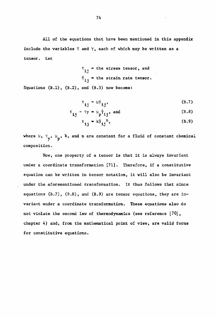
All of the equations that have been mentioned in this appendix

include the variables T and Y, each of which may be written as a

tensor. Let

T., = the stress tensor, and ij

43

Equations (B.1), (B.2), and (B.3) now become:

= the strain rate tensor.

"54 = Wa? (B.7)

Ts - Ty = Wve and (B.8)

57 ky, 5" (B.9)

where U, Ty Hos k, and n are constant for a fluid of constant chemical

composition.

Now, one property of a tensor is that it is always invariant

under a coordinate transformation [71]. Therefore, if a constitutive

equation can be written in tensor notation, it will also be invariant

under the aforementioned transformation. It thus follows that since

equations (B.7), (B.8), and (B.9) are tensor equations, they are in~

variant under a coordinate transformation. These equations also do

not violate the second law of thermodynamics (see reference [70],

chapter 4) and, from the mathematical point of view, are valid forms

for constitutive equations.

Appendix C

Wells-Brookfield Theory

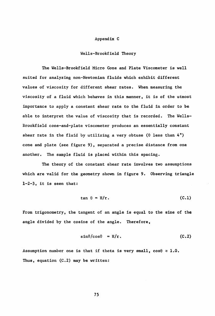
The Wells-Brookfield Micro Cone and Plate Viscometer is well

suited for analyzing non-Newtonian fluids which exhibit different

values of viscosity for different shear rates. When measuring the

viscosity of a fluid which behaves in this manner, it is of the utmost

importance to apply a constant shear rate to the fluid in order to be

able to interpret the value of viscosity that is recorded. The Wells-

Brookfield cone-and-plate viscometer produces an essentially constant

shear rate in the fluid by utilizing a very obtuse (@ less than 4°)

cone and plate (see figure 9), separated a precise distance from one

another. The sample fluid is placed within this spacing.

The theory of the constant shear rate involves two assumptions

which are valid for the geometry shown in figure 9. Observing triangle

1-2-3, it is seen that:

tan 6 = H/r. (c.1)

From trigonometry, the tangent of an angle is equal to the sine of the

angle divided by the cosine of the angle. Therefore,

sinO/cos® = H/r. (C.2)

Assumption number one is that if theta is very small, cosO ~ 1.0.

Thus, equation (C.2) may be written:

75

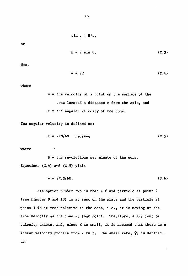
76

sin 6 = H/r,

or

H = r sin @, (C.3)

Now,

v= rw (C.4)

where

v = the velocity of a point on the surface of the

cone located a distance r from the axis, and

W = the angular velocity of the cone.

The angular velocity is defined as:

W = 27N/60 + rad/sec (C.5)

where

N = the revolutions per minute of the cone.

Equations (C.4) and (C.5) yield

v = 2trN/60. (C.6)

Assumption number two is that a fluid particle at point 2

(see figures 9 and 10) is at rest on the plate and the particle at

point 3 is at rest relative to the cone, i.e., it is moving at the

same velocity as the cone at that point. Therefore, a gradient of

velocity exists, and, since H is small, it is assumed that there is a

linear velocity profile from 2 to 3. The shear rate, Y, is defined

as;

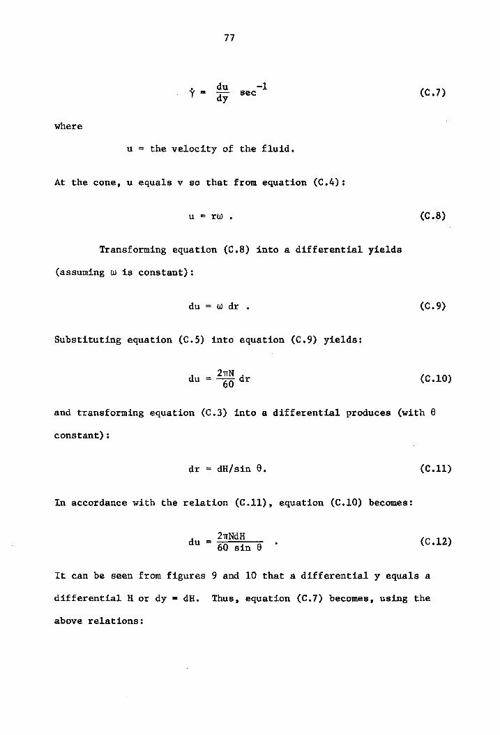
7]

Y= ay sec (C.7)

where

u = the velocity of the fluid.

At the cone, u equals v so that from equation (C.4):

Transforming equation (C.8) into a differential yields

(assuming w is constant):

du =wdr. (c.9)

Substituting equation (C.5) into equation (C.9) yields:

_ 27N du = “Go dF (C.10)

and transforming equation (C.3) into a differential produces (with 6

constant):

dr = dH/sin 9. (c.11)

In accordance with the relation (C.11), equation (C.10) becomes:

21NdH du = 60 sind (C.12)

It can be seen from figures 9 and 10 that a differential y equals a

differential H or dy = dH. Thus, equation (C.7) becomes, using the

above relations:

78

du | 20 Y " dy ~ 60 sin 0

or

60 sin 6 sec . (C.13)

Notice that in equation (C.13) the shear rate is a function only of N.

Since N is the revolutions per minute of the cone, by keeping N con-

stant, a constant shear rate will be developed in the fluid.

The derivation of the shear stress begins by observing in

triangle 3-4-5 (figure 9) that:

d2 = dr/cos 6. (C.14)

Now, from figure ll, __

AB = rdq. (C.15)

Similarly, — CD = (r + d&) do

= rdd + ddd, (C.16)

where did may be neglected because it is of a smaller order of magni-

tude compared to rd?. From equations (C.15) and (C.16) we arrive at

the conclusion that AB ~ CD and it therefore follows that

dA = rdgd&. (C.17)

Substituting d2& from equation (C.14) into equation (C.17) yields,

da = Tdddr (c.18) cos 6 °

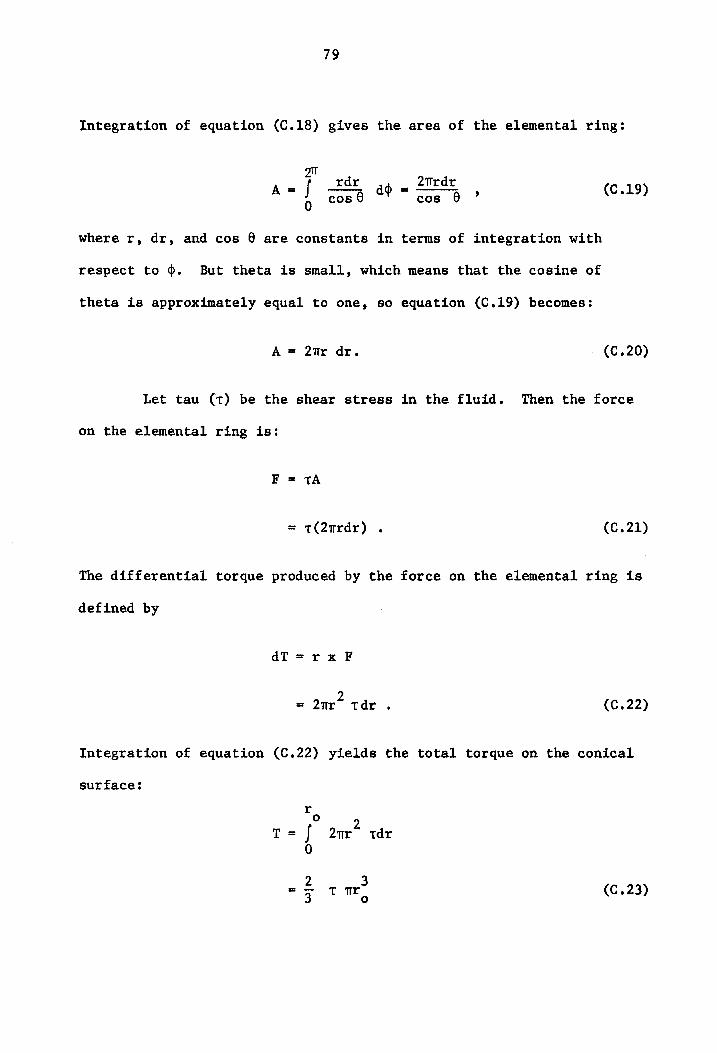
79

Integration of equation (C.18) gives the area of the elemental ring:

rdr = 2Trdr

An J co56 &" cos 6 ° (C.19) where r, dr, and cos 9 are constants in terms of integration with

respect to >. But theta is small, which means that the cosine of

theta is approximately equal to one, so equation (C.19) becomes:

A = 2tr dr. (C.20)

Let tau (t) be the shear stress in the fluid. Then the force

on the elemental ring is:

F = TA

= (2trdr) . (C.21)

The differential torque produced by the force on the elemental ring is

defined by

dT=rxF

= onr? tdr . (C.22)

Integration of equation (C.22) yields the total torque on the conical

surface;

= = Tt 1r (C.23)

80

where T is assumed not to vary with r if the shear rate does not.

Solving equation (C.23) for T gives:

3T

2mr 3 oO

(C.24)

Observe that equation (C.24) for T is a function of T, the torque

applied to the cone. Thus, by applying a constant torque to the cone,

the shear stress in the fluid will also be constant.

Equations (C.13) and (C.24) include several known quantities:

@ (cone angle) = 1.565°,

ri 2.409 cm., and

Tw = 3.14159.

The torque (T) in equation (C.24) may be expressed as follows:

[ = B'T* (C.25)

where

B' = a fraction of T*, and

T* = the total torque that can be developed

by the viscometer (673.7 dynes-cm.).

‘ Let

' 2 B= B'xi0 , (C.26)

so that B is the direct numerical reading in percent of total torque

from the viscometer dial. Then, substituting the values of 6, To TT,

81

and T* given above into equations (C.13) and (C.24), we obtain:

¥ = 3.88 N sec, and

2 t = 0.2327 B dynes/cm .

Finally, the apparent viscosity is defined as:

w= Ty.

Substituting equations (C.27) and (C.28) into (C.29) yields:

us = 0.06B/N poise

or

w= 6B/N centipoise .

(C.27)

(C.28)

(C.29)

(C.30)

(C.31)

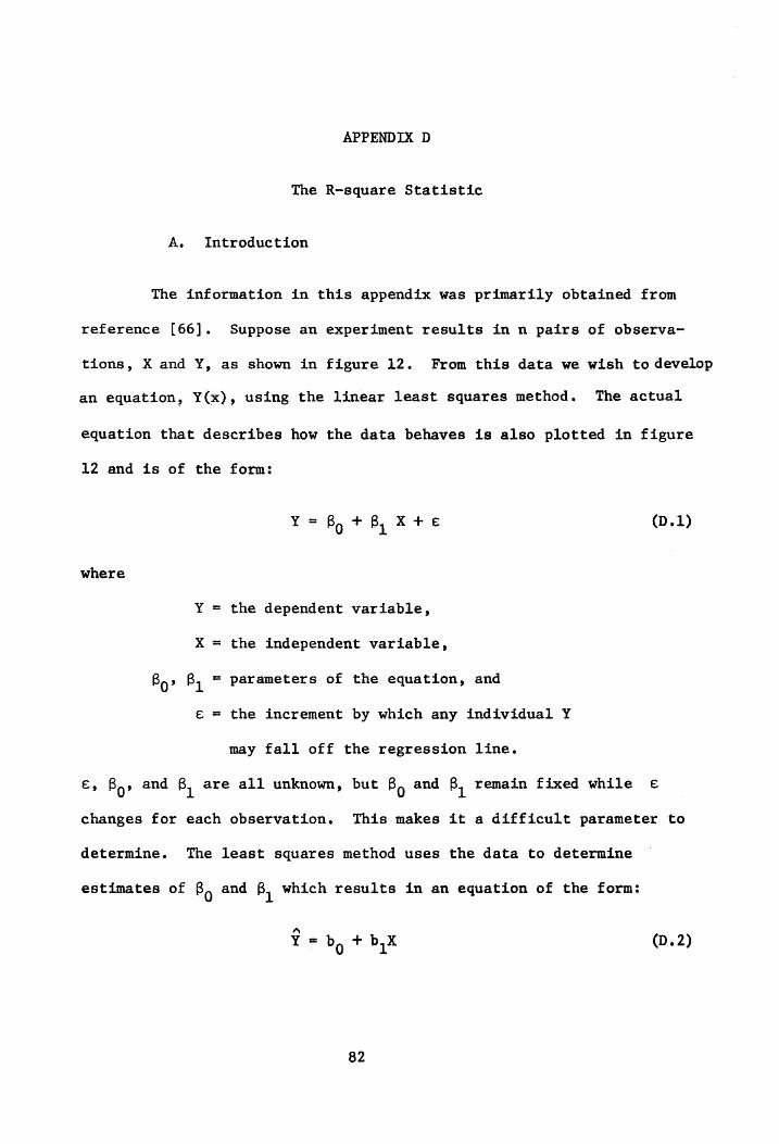
APPENDIX D

The R-square Statistic

A. Introduction

The information in this appendix was primarily obtained from

reference [66]. Suppose an experiment results in n pairs of observa-

tions, X and Y, as shown in figure 12. From this data we wish to develop

an equation, Y(x), using the linear least squares method. The actual

equation that describes how the data behaves is also plotted in figure

12 and is of the form:

Y= 6, +8, Xt+e (D.1)

where

Y = the dependent variable,

X = the independent variable,

Bo» By = parameters of the equation, and

m i the increment by which any individual Y

may fall off the regression line.

Ee, Bos and B. are all unknown, but By and B, remain fixed while ¢€

changes for each observation. This makes it a difficult parameter to

determine. The least squares method uses the data to determine

estimates of By and By which results in an equation of the form:

A

Y= by + b,x (D.2)

82

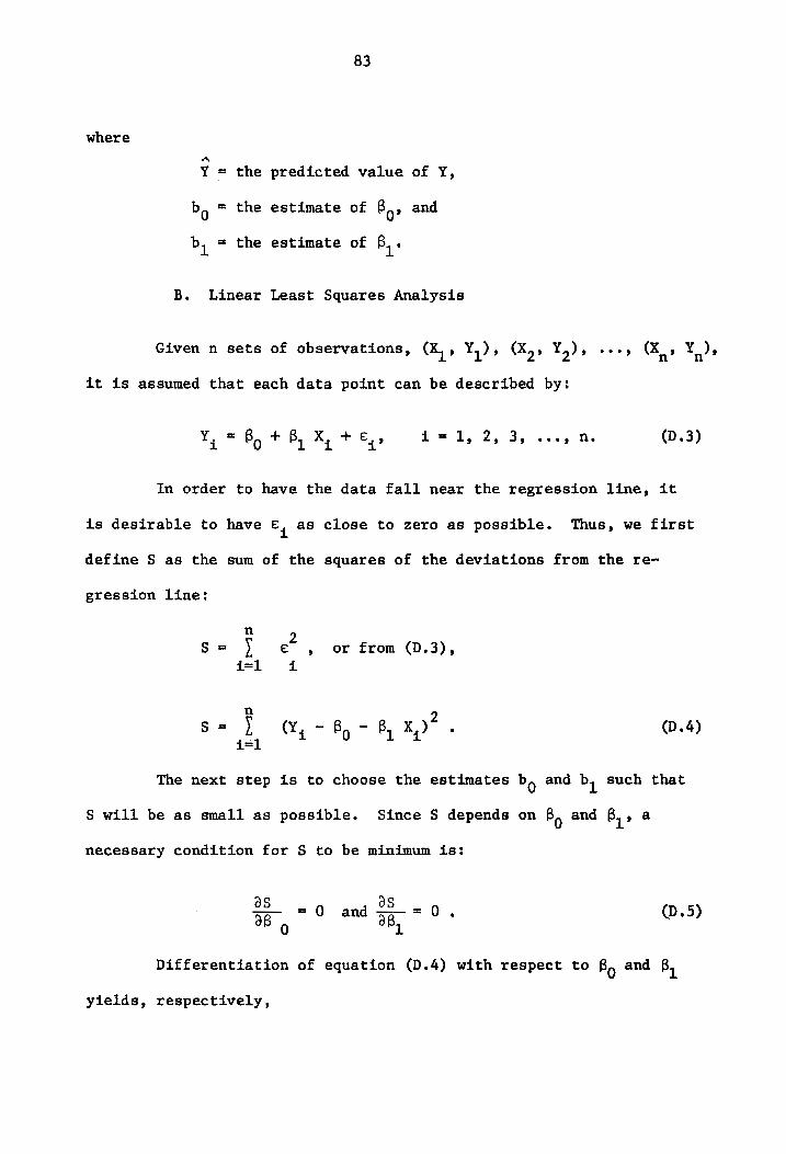
83

where

Aw

Y = the predicted value of Y,

a n the estimate of Bo» and

o il the estimate of Bi.

B. Linear Least Squares Analysis

Given n sets of observations, (X_, YX)» (X,, Y,)> cee, > yw?

it is assumed that each data point can be described by:

¥, = By + 8, X, +; i=l, 2; 3; eeesg The (D.3)

In order to have the data fall near the regression line, it

is desirable to have €, as close to zero as possible. Thus, we first i

define S as the sum of the squares of the deviations from the re-

gression line:

sS= } 7 ,» or from (0.3), =1 i

a 2 s= } (, - 8) - 6, X,)° . (D.4) 1=1

The next step is to choose the estimates bo and by such that

S will be as small as possible. Since S depends on By and By» a

necessary condition for S to be minimum is:

0s __ = Q and 0S

0

8B, = 0 e (D.5)

Differentiation of equation (D.4) with respect to By and B,

yields, respectively,

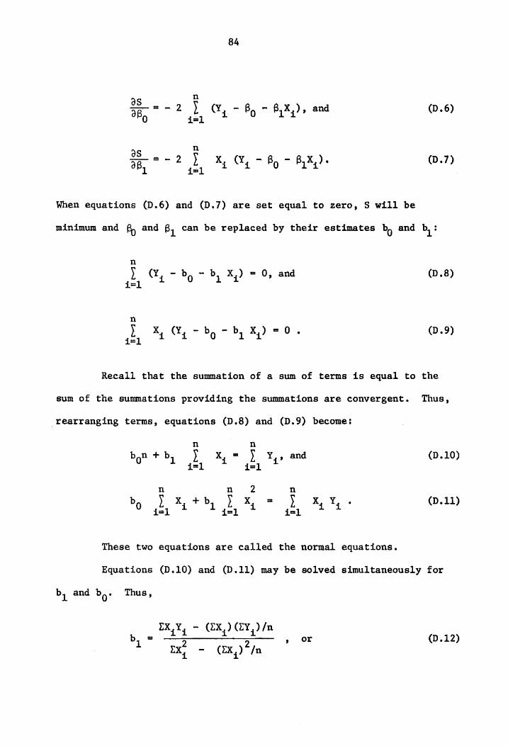
84

Se 2 } cy, - 65 - 8,X,), and 0.6) 0 i=l

oR 2 } XK, Oy - By - ByX,). @.7) 1 i=1

When equations (D.6) and (D.7) are set equal to zero, S will be

minimum and By and By can be replaced by their estimates b, and b,: 0 1

n

Y. Gy - by - by X,) = 0, and (D.8) i=l

Th

oy Xp Mp Pg by Hy) =O. (D.9)

Recall that the summation of a sum of terms is equal to the

sum of the summations providing the summations are convergent. Thus,

rearranging terms, equations (D.8) and (D.9) become:

n n

b,n + b y xX, = J} y,, and (D.10) 0 a ft, a A Tt

} Pye | b X, +b xX, = X, Y¥, .- (D.11) 0 1=1 i 1 i=1 i i=] 1 i

These two equations are called the normal equations.

Equations (D.10) and (D.11) may be solved simultaneously for

by and bo: Thus,

EX, ¥

4

- (2X,) (ZY,)/n

- (Ex,)7/n

; or (D.12)

L

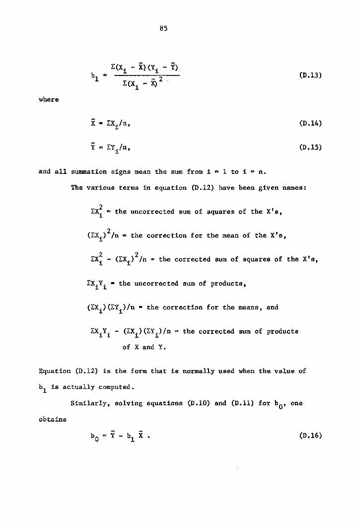
85

EQ, - X)Qy - ¥). b - (D.13)

1 Ea, - % 2

where

X = EX, /n, (D.14)

Y= rY,/n, (D.15)

and all summation signs mean the sum from i= 1totie=n.

The various terms in equation (D.12) have been given names:

Ex, = the uncorrected sum of squares of the X's,

(2x,)?/a = the correction for the mean of the X's,

Ix, - (X,)°/n = the corrected sum of squares of the X's,

EX,Y, = the uncorrected sum of products,

(ZX, ) (ZY, )/n = the correction for the means, and

UX ,Y, - (2X, ) GY) /n = the corrected sum of products

of X and Y.

Equation (D.12) is the form that is normally used when the value of

b) is actually computed.

Similarly, solving equations (D.10) and (D.11) for bo» one

obtains

86

Substituting equation (D.16) into (D.2) results in;

“ — on

where by is defined by either equation (D.12) or (D.13).

Equation (D.17) is the linear least squares equation for a set

of n observations, But this equation is not an exact equation since

the plot (figure 12) shows that not all of the data points lie on the

regression line. There is thus an error inherent in the least squares

method. This error may be presented in several forms. The form to be

used in this analysis will be the R-square statistic.

C. The Precision of the Estimated Regression-—-the R-square Statistic

First we define the residual to be the actual data point value

minus the value predicted by the regression line:

nN

Residual = Y, - Y, . (D.18)

When there is a By term, the sum of the residuals is always equal to

zero, i.e., the distribution of data points on one side of the

regression line is exactly balanced and cancelled by that on the

other side. The omission of the By term implies that the response is

zero when all independent variables are zero.

Now consider the following identity:

aA ~ A —

¥,7¥,*Y,-¥- @,-¥).. (D.19)

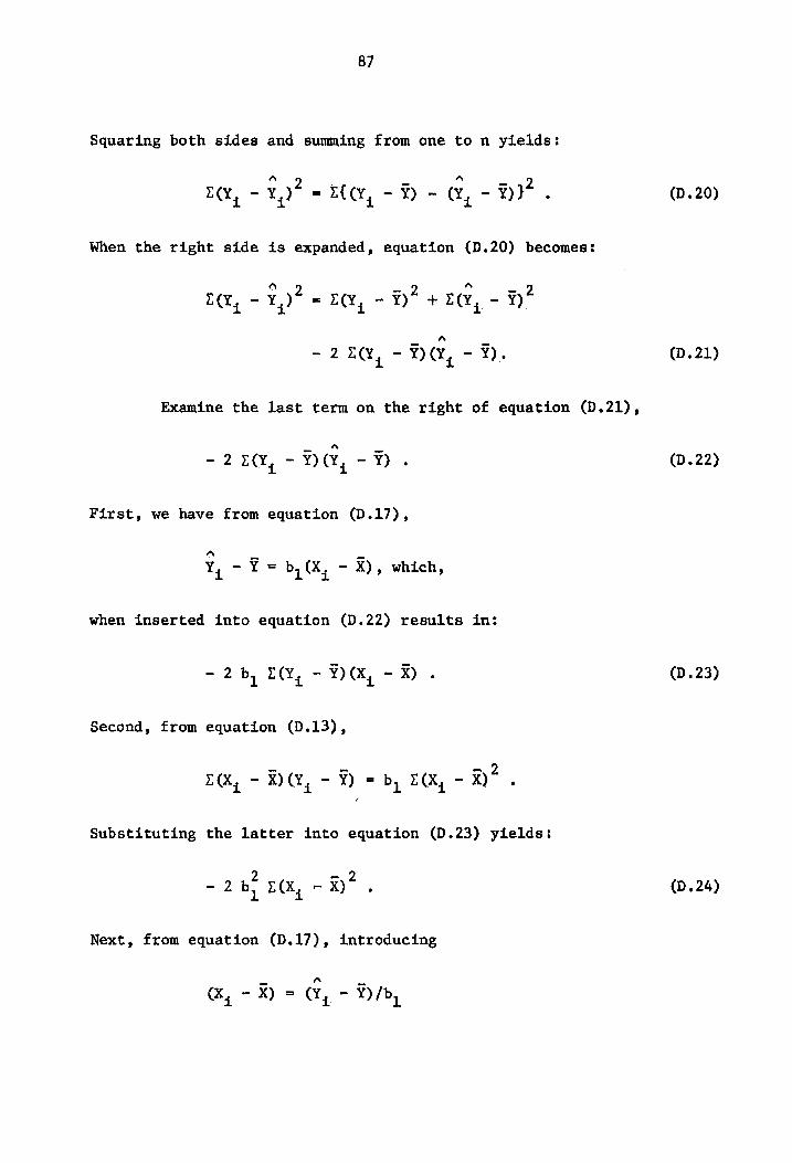
87

Squaring both sides and summing from one to n yields:

Nn

EC, = x,)° - Ha, -% - a, - x} . (D .20)

When the right side is expanded, equation (D.20) becomes:

“ 2 =. 2 “ =. 2 a, - ¥,) = EM, - Y) + =, Y)

- 22, - ¥) (xX, - ¥). (D.21)

Examine the last term on the right of equation (D.21),

- 22, - ¥) (Y, - ¥). (D.22)

First, we have from equation (D.17),

A _ ~

¥y 7 Y= b, &, - X), which,

when inserted into equation (D.22) results in:

~ 2 by EY, - YX) (XK, - xX). (D.23)

Second, from equation (D.13),

E(x, - X)(¥Y, - ¥) = b, L(X, - x)? i i 1 i ,

Substituting the latter into equation (D.23) yields:

2 =. 2 - 2b; 5%, - x)". (D.24)

Next, from equation (D.17), introducing

a, - = 4, -H/,

88

into equation (D.24) will produce

- 2 rr, ~ 7)" , (D.25)

Thus, replacing the third term on the right of equation (D.21) with

(D.25) and rearranging terms results in:

=. 2 a 2 EW, - ¥)° = Lqy, - ¥,) + rq, - 37, (D.26)

The terms in equation (D.26) are defined as:

zM, - 7)? = the sum of squares of deviations

about the mean (S.S.M.),

EY, - x,)" = the sum of squares of deviations about the

regression line (S.S.A.R.) or the sum of

the squares of the residuals, and

zy - z)? = the sum of squares of deviations of the

predicted values from the mean due to

regression (S.S.D.R.).

Thus equation (D.26) reads:

S.S.M. = &.S.A.R. + S.S.D.R. . (D.27)

Ideally we would like each predicted value of Y to be equal to the

actual value:

>

which is the same as saying that the residuals should be as small as

possible. In terms of equation (D.27), it is desirable to have:

89

S.S.A.R. 70. (D.29)

When S.S.A.R. is approximately zero:

S.S.M. ~ S.S.D.R. . (D.30)

Dividing both sides of equation (D.30) by S.S.M. yields:

Thus, we define the R-square statistic as:

nC, - %)? oF ° (D.32)

rq, - ¥) R-square =

Expressing equation (D.32) in words, we would say that the

R-square statistic is the ratio of the sum of squares of deviations

of the predicted values from the mean to the sum of squares of

deviations about the mean. nw

When the fit is perfect (i.e., Y, = ¥, and therefore no i

residuals), the R-square statistic is equal to one. As the predicted

values deviate from the actual values, the R-square statistic becomes

less and less, until finally, if there is no relation between the

predicted values and the actual values, the R-square statistic is

equal to zero.

The R-square statistic is a convenjent measure of the signifi-

cance of the estimated regression equation because it includes only

one assumption, that is, a linear least squares method is used to

90

compute the regression equation.

VITA

The author was born in Cumberland, Maryland on February 7,

1951. He attended Parkside Elementary School and graduated from

Allegany High School in 1969. From 1969 until 1973 he attended

Virginia Polytechnic Institute and State University where he obtained

a B.S. in Engineering Science and Mechanics in September. After

graduation he began graduate studies at the same university and

department. He has worked as a graduate teaching assistant and is

currently working as a graduate research assistant and plans to

continue his studies with a Ph.D. degree as his goal.

“Piradnuz Se Walla Frederick J. Walburn

91

AN EMPIRICAL CONSTITUTIVE EQUATION FOR

ANTICOAGULATED HUMAN BLOOD

by

Frederick James Walburn

(ABSTRACT)

A constitutive equation for whole human blood was developed

using a power law functional form. This power law equation contains

two parameters, the consistency index and the non-Newtonian index for

the fluid. Viscometric data, utilizing a cone and plate viscometer,

were obtained from anticoagulated blood samples of known hematocrit

levels and chemical compositions. A multiple regression technique

with apparent viscosity as the dependent variable was used to deter-

mine the consistency index and the non-Newtonian index.

A model including only the shear rate as the independent

variable was found to be lacking any substantial degree of signifi-

cance. When hematocrit was added as an independent variable, the

degree of fit increased considerably.

Of the chemical variables examined, the least significant,

as far as effects on viscosity is concerned, were the plasma lipids.

The proteins, fibrinogen and globulin were found to have a much

greater effect on viscosity than the protein, albumin. The best

constitutive equation involving the chemical composition of blood

was found to include the shear rate, the hematocrit level, and a

variable which is the sum of fibrinogen and globulin. This model

produced a statistically significant increase in the correlation

between experimental and theoretical data compared with the best two

variable model.