An empirical analysis of aggregate household portfolios

Available online at www.sciencedirect.com

www.elsevier.com/locate/jbf

Journal of Banking & Finance 32 (2008) 1583–1597

An empirical analysis of aggregate household portfolios

Michel Normandin a,*, Pascal St-Amour b,1

a Department of Economics and CIRPEE, HEC Montreal, 3000 Chemin de la Cote-Ste-Catherine, Montreal, Quebec, Canada H3T 2A7b HEC University of Lausanne, Swiss Finance Institute, HEC Montreal, CIRANO, and CIRPEE, University of Lausanne, CH-1015 Lausanne, Switzerland

Received 13 February 2007; accepted 22 November 2007Available online 11 January 2008

Abstract

This paper analyzes the important time variation in US aggregate household portfolios. To do so, we first use flexible descriptions ofpreferences and investment opportunities to derive household optimal decision rules that nest static, myopic, and non-myopic portfolioallocations. We then compare these rules to the data through formal statistical analysis. Our main results reveal that: (i) static and myo-pic investment behaviors are rejected, (ii) non-myopic portfolio allocations are supported, and (iii) the Fama–French factors best explainempirical portfolio shares.� 2007 Elsevier B.V. All rights reserved.

JEL classification: G11; G12

Keywords: Dynamic hedging positions; Generalized recursive preferences; Static, Myopic, and Non-myopic portfolio allocations; Time-varying invest-ment opportunity set

1. Introduction

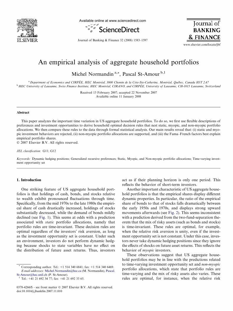
One striking feature of US aggregate household port-folios is that holdings of cash, bonds, and stocks relativeto wealth exhibit pronounced fluctuations through time.Specifically, from the mid 1970s to the late 1980s the empiri-cal share of cash drastically increased, holdings of stockssubstantially decreased, while the demand of bonds mildlydeclined (see Fig. 1). This seems at odds with a predictionassociated with static portfolio allocations, namely thatportfolio rules are time-invariant. These decision rules areoptimal regardless of the investors’ risk aversion, as longas the investment opportunity set is constant. Under suchan environment, investors do not perform dynamic hedg-ing because shocks to state variables have no effect onthe distribution of future asset returns. Thus, investors

0378-4266/$ - see front matter � 2007 Elsevier B.V. All rights reserved.

doi:10.1016/j.jbankfin.2007.11.010

* Corresponding author. Tel.: +1 514 340 6841; fax: +1 514 340 6469.E-mail addresses: [email protected] (M. Normandin), Pascal.

[email protected] (P. St-Amour).1 Tel.: +41 21 692 34 77; fax: +41 21 692 33 65.

act as if their planning horizon is only one period. Thisreflects the behavior of short-term investors.

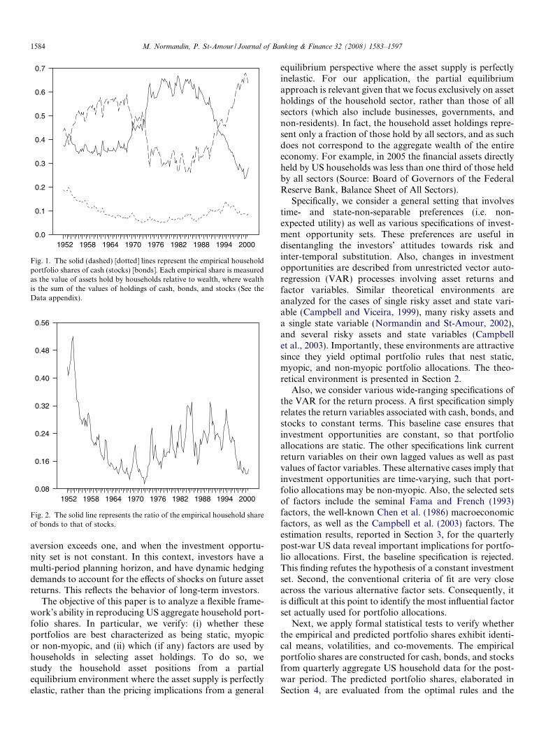
Another important characteristic of US aggregate house-hold portfolios is that the empirical shares display differentdynamic properties. In particular, the ratio of the empiricalshare of bonds to that of stocks falls dramatically betweenthe early 1950s and 1970s, and displays strong upwardmovements afterwards (see Fig. 2). This seems inconsistentwith a prediction derived from the two-fund-separation the-orem that the mix of risky assets (such as bonds and stocks)is time-invariant. These rules are optimal, for example,when the relative risk aversion is unity, even if the invest-ment opportunity set is not constant. Under this case, inves-tors never take dynamic hedging positions since they ignorethe effects of shocks on future asset returns. This reflects thebehavior of myopic investors.

These observations suggest that US aggregate house-hold portfolios may be in line with the predictions relatedto time-varying investment opportunity set and non-myopic

portfolio allocations, which state that portfolio rules aretime-varying and the mix of risky assets also varies. Theserules are optimal, for instance, when the relative risk

mailto:[email protected]



1952 1958 1964 1970 1976 1982 1988 1994 20000.0

0.1

0.2

0.3

0.4

0.5

0.6

0.7

Fig. 1. The solid (dashed) [dotted] lines represent the empirical householdportfolio shares of cash (stocks) [bonds]. Each empirical share is measuredas the value of assets hold by households relative to wealth, where wealthis the sum of the values of holdings of cash, bonds, and stocks (See theData appendix).

1952 1958 1964 1970 1976 1982 1988 1994 20000.08

0.16

0.24

0.32

0.40

0.48

0.56

Fig. 2. The solid line represents the ratio of the empirical household shareof bonds to that of stocks.

1584 M. Normandin, P. St-Amour / Journal of Banking & Finance 32 (2008) 1583–1597

aversion exceeds one, and when the investment opportu-nity set is not constant. In this context, investors have amulti-period planning horizon, and have dynamic hedgingdemands to account for the effects of shocks on future assetreturns. This reflects the behavior of long-term investors.

The objective of this paper is to analyze a flexible frame-work’s ability in reproducing US aggregate household port-folio shares. In particular, we verify: (i) whether theseportfolios are best characterized as being static, myopicor non-myopic, and (ii) which (if any) factors are used byhouseholds in selecting asset holdings. To do so, westudy the household asset positions from a partialequilibrium environment where the asset supply is perfectlyelastic, rather than the pricing implications from a general

equilibrium perspective where the asset supply is perfectlyinelastic. For our application, the partial equilibriumapproach is relevant given that we focus exclusively on assetholdings of the household sector, rather than those of allsectors (which also include businesses, governments, andnon-residents). In fact, the household asset holdings repre-sent only a fraction of those hold by all sectors, and as suchdoes not correspond to the aggregate wealth of the entireeconomy. For example, in 2005 the financial assets directlyheld by US households was less than one third of those heldby all sectors (Source: Board of Governors of the FederalReserve Bank, Balance Sheet of All Sectors).

Specifically, we consider a general setting that involvestime- and state-non-separable preferences (i.e. non-expected utility) as well as various specifications of invest-ment opportunity sets. These preferences are useful indisentangling the investors’ attitudes towards risk andinter-temporal substitution. Also, changes in investmentopportunities are described from unrestricted vector auto-regression (VAR) processes involving asset returns andfactor variables. Similar theoretical environments areanalyzed for the cases of single risky asset and state vari-able (Campbell and Viceira, 1999), many risky assets anda single state variable (Normandin and St-Amour, 2002),and several risky assets and state variables (Campbellet al., 2003). Importantly, these environments are attractivesince they yield optimal portfolio rules that nest static,myopic, and non-myopic portfolio allocations. The theo-retical environment is presented in Section 2.

Also, we consider various wide-ranging specifications ofthe VAR for the return process. A first specification simplyrelates the return variables associated with cash, bonds, andstocks to constant terms. This baseline case ensures thatinvestment opportunities are constant, so that portfolioallocations are static. The other specifications link currentreturn variables on their own lagged values as well as pastvalues of factor variables. These alternative cases imply thatinvestment opportunities are time-varying, such that port-folio allocations may be non-myopic. Also, the selected setsof factors include the seminal Fama and French (1993)factors, the well-known Chen et al. (1986) macroeconomicfactors, as well as the Campbell et al. (2003) factors. Theestimation results, reported in Section 3, for the quarterlypost-war US data reveal important implications for portfo-lio allocations. First, the baseline specification is rejected.This finding refutes the hypothesis of a constant investmentset. Second, the conventional criteria of fit are very closeacross the various alternative factor sets. Consequently, itis difficult at this point to identify the most influential factorset actually used for portfolio allocations.

Next, we apply formal statistical tests to verify whetherthe empirical and predicted portfolio shares exhibit identi-cal means, volatilities, and co-movements. The empiricalportfolio shares are constructed for cash, bonds, and stocksfrom quarterly aggregate US household data for the post-war period. The predicted portfolio shares, elaborated inSection 4, are evaluated from the optimal rules and the

M. Normandin, P. St-Amour / Journal of Banking & Finance 32 (2008) 1583–1597 1585

VAR processes associated with the various sets of factors.The test results highlight two key implications for theassessment of portfolio allocations. First, the variousmoments of the empirical portfolio shares are never repli-cated from the baseline specification, nor from the combi-nations of any alternative factor sets with a relative riskaversion of one. This empirical evidence refutes both staticand myopic investment behaviors. Second, the propertiesof the empirical portfolio shares are best explained by com-bining the Fama–French factors with reasonable values ofrelative risk aversion larger than unity. This providesempirical support for non-myopic portfolio allocations.

For completeness, we perform statistical tests to checkwhether the empirical and predicted consumption sharesdisplay the same means and volatilities. The empirical con-sumption share is constructed as the consumption-wealthratio from quarterly aggregate US data for the post-warperiod. The predicted consumption shares, explained inSection 5, are evaluated from the optimal consumption ruleand the VAR processes associated with the baseline andFama–French specifications. The test results reveal twoimportant implications for the evaluation of portfolio allo-cations. First, the moments of the empirical consumptionshare are never reproduced from the baseline specification,nor from the combination of the Fama–French factors witha relative risk aversion of one. This provides additionalevidence against static and myopic portfolio allocations.Second, the properties of the empirical consumption sharecan be recovered by combining the Fama–French specifica-tion with reasonable values of relative risk aversion largerthan unity. This provides additional evidence in favor ofnon-myopic portfolio allocations.

Altogether, the return, portfolio, and consumption anal-yses lead to key conclusions for US aggregate householdportfolio allocations. First, there is a clear rejection of sta-tic and myopic investment behaviors. Second, there is anempirical support for non-myopic portfolio allocations.Third, there is some evidence suggesting that the Fama–French factors are those which best explain empirical port-folio shares.

2. Theoretical environment

This section presents the household’s problem, specifiesthe dynamics of the state variables, and explains theapproximate consumption and portfolio decision rules.

2.1. Household’s problem

We consider the following household’s problem:

ut ¼ maxfct ;ai;tgnr

i¼2

ð1� dÞcw�1w

t þ dðEtu1�ctþ1 Þ

w�1wð1�cÞ

� � ww�1

; ð1Þ

s:t: wtþ1 ¼ ð1þ rp;tþ1Þðwt � ctÞ; ð2Þ

rp;tþ1 ¼ r1;tþ1 þXnr

i¼2

ai;txri;tþ1: ð3Þ

The term Et denotes the expectation operator conditionalon information available in period t, ut is the within-periodutility, ct is real consumption, wt is real wealth, rp;tþ1 is thereal (net) return on the wealth portfolio, r1;tþ1 is the real(net) return for a benchmark risky asset, ri;tþ1 is the real(net) return for an alternative risky asset i, whilexri;tþ1 ¼ ðri;tþ1 � r1;tþ1Þ and ai;t are the associated excessreturn (relative to the benchmark return) and portfolioshare, with asset i ¼ 2; . . . ; nr. Also, 0 < d < 1 is a timediscount factor, c > 0 is the relative risk aversion, w > 0is the elasticity of inter-temporal substitution, and nr isthe number of risky assets.

Eq. (1) describes the preferences of an infinitely-livedrepresentative household from a generalized recursive util-ity function (Epstein and Zin, 1989; Weil, 1990). Therestriction c ¼ w�1 yields the standard state- and time-sep-arable Von Neumann-Morgenstern preferences. Thisimplies that the household is indifferent to the timing ofthe resolution of uncertainty (of the temporal lottery overconsumption). Conversely, c 6¼ w�1 yields non-separablepreferences. In particular, the agent prefers an early (late)resolution of uncertainty when c > w�1ðc < w�1Þ. Eq. (2)represents the usual inter-temporal budget constraint. Eq.(3) defines the wealth portfolio return from the benchmarkand excess returns and from the restriction that the portfo-lio shares of all assets sum to unity.

The problem (1)–(3) stipulates that the current con-sumption and contemporaneous portfolio shares corre-spond to the household’s choice variables. Also, thecurrent wealth is a predetermined variable, while futurebenchmark and excess returns are exogenous variables.

2.2. Dynamics of the state variables

We specify the law of motion describing the dynamics ofthe state variables as:

stþ1 ¼ U0 þU1st þ vtþ1;

vtþ1 � NIDð0;RÞ:ð4Þ

Here, stþ1 ¼ r0tþ1 f 0tþ1

� �0is the ðns � 1Þ vector of state

variables, rtþ1 is the ðnr � 1Þ vector of return variableswhich includes the benchmark and excess returns, f tþ1 isthe ðnf � 1Þ vector of factor variables which contains addi-tional exogenous variables, and vtþ1 is the ðns � 1Þ vector ofstate-variable innovations which are assumed to follow anormal distribution with zero means and a homoscedasticstructure. Also, U0 is the ðns � 1Þ vector of intercepts andU1 is the ðns � nsÞ matrix of slope coefficients.

Eq. (4) is a first-order vector autoregressive (VAR) pro-cess. A baseline specification of this process imposes theabsence of dynamic feedbacks between future and currentstate variables ðU1 ¼ 0Þ. These restrictions yield a constantinvestment opportunity set; i.e. the return variables areindependently and identically distributed. The baselinespecification will be useful shortly to study static portfolioallocations.


The alternative specifications of the VAR processcapture the dependence of future return variables on theirpresent values as well as on current factor variablesðU1 6¼ 0Þ. Our selected specifications will involve differentfactors, which are among the most widely used in theempirical asset-pricing literature, and which are well-known to have predictive power on returns. These specifi-cations lead to time-varying investment opportunity sets.Again, this will prove to be useful below to study myopicand non-myopic portfolio allocations.

2.3. Decision rules

The shares are defined as the ratios of consumption andportfolio relative to wealth:

ac;t �ct

wt; ð5Þ

ai;t �wi;t

wt; ð6Þ

where ac;t is the consumption share of wealth, wt ¼Pnri¼1wi;t, while ai;t and wi;t are the portfolio share and the

value of asset i, with i ¼ 1; . . . ; nr.The optimal decision rules associated with the house-

hold’s problem (1)–(3) and the VAR process (4) relatethe shares (5) and (6) to the contemporaneous state vari-ables. Unfortunately, the exact analytical solution isunknown for general values of the parameters describingthe preferences of the household and the dynamics of thestate variables. We circumvent this problem by approxi-mating the decision rules from the numerical proceduredeveloped in Campbell et al. (2003).

In brief, the approximation of the decision rules firstrelates the portfolio return to asset returns; this holdsexactly in continuous time. The approximation also log-linearizes the budget constraint around the unconditionalexpectation of the log consumption share; this holdsexactly for constant consumption shares. The approxima-tion then relies on a second-order Taylor expansion ofthe Euler equations around the conditional expectationsof consumption growth and returns; this holds exactlywhen the variables are conditionally normally distributed.The approximation is finally obtained by solving a recur-sive non-linear equation system whose coefficients are com-plex functions of the parameters involved in the preferences(1) and the VAR process (4). Whereas the system can besolved analytically when there is a unique state variableaffecting a single risky asset return (Campbell and Viceira,1999) or many risky asset returns (Normandin andSt-Amour, 2002), it must be solved numerically in ourmultiple states and risky assets environment.

The solution establishes that the logarithm of the con-sumption share and the portfolio shares are respectivelyquadratic and affine in the state variables:

logðac;tÞ ¼ b0 þ B01st þ s0tB2st; ð7Þai;t ¼ a0i þ A01ist; ð8Þ

a1;t ¼ 1�Xnr

i¼2

ai;t: ð9Þ

The terms b0 and a0i are scalars, B2 is a ðns � nsÞ lowertriangular matrix, whereas B1 and A1i are ðns � 1Þ vectors,with i ¼ 2; . . . ; nr. As mentioned above, these terms dependon the preference parameters d, w, and c in (1) and on theVAR parameters U0, U1, and R in (4), and are solvednumerically.

Campbell and Koo (1997) show for the case of a singlestate variable that the approximation (7)–(9) is very precise,especially when the consumption share is not excessivelyvolatile. Furthermore, the approximation nests the knownexact analytical solutions obtained under myopic consump-tion behavior ðw ¼ 1Þ where the consumption share isconstant, myopic portfolio allocation ðc ¼ 1Þ where thedemand for dynamic hedging portfolios is zero, and con-stant investment opportunity sets ðU1 ¼ 0Þ (Giovanniniand Weil, 1989).

It is worth stressing that the myopic consumption andportfolio rules become optimal for all values of w and cwhen the investment opportunities are constant ðU1 ¼ 0Þ.That is, the household chooses consumption and theportfolio as if the planning horizon is only one period. Con-sequently, the household selects a fixed consumption share,regardless of its elasticity of inter-temporal substitution.Furthermore, the household never takes dynamic hedgingpositions, whatever its risk aversion. This behavior reflectsthe static portfolio allocation of a short-term investor.

In contrast, non-myopic rules are optimal for w 6¼ 1 andc 6¼ 1, and when the investment opportunities are time-varying ðU1 6¼ 0Þ. In this case, the household forms deci-sions from a planning horizon that exceeds one period.As a result, the household chooses a consumption sharethat varies through time, as long as its elasticity of inter-temporal substitution differs from unity. Moreover, thehousehold performs inter-temporal hedging to reduce itsexposure to adverse changes in investment opportunities,as long as its risk aversion is larger than unity. This hedg-ing behavior reflects the non-myopic portfolio allocation ofa long-term investor.

In our analysis, we compare the decision rules (8) and(9) associated with the baseline and various alternativespecifications of the VAR process (4) in order to verify (i)whether actual portfolios are static, myopic or non-myo-pic, and (ii) which (if any) factors are used by householdsin selecting asset holdings.

3. Return analysis

In this section, we estimate various specifications of theVAR process (4). We concentrate our attention on cash,bonds, and stocks. Given our objective, the specificationsalways include observable measures of return variablesrelated to these assets. In particular, the return on cash isdefined as the benchmark, r1;tþ1, and is measured as the real


(net) ex post return on short-term Treasury bills, rtb;tþ1.Moreover, the excess returns, xri;tþ1, are measured forbonds, xrb;tþ1, and for stocks, xrs;tþ1.

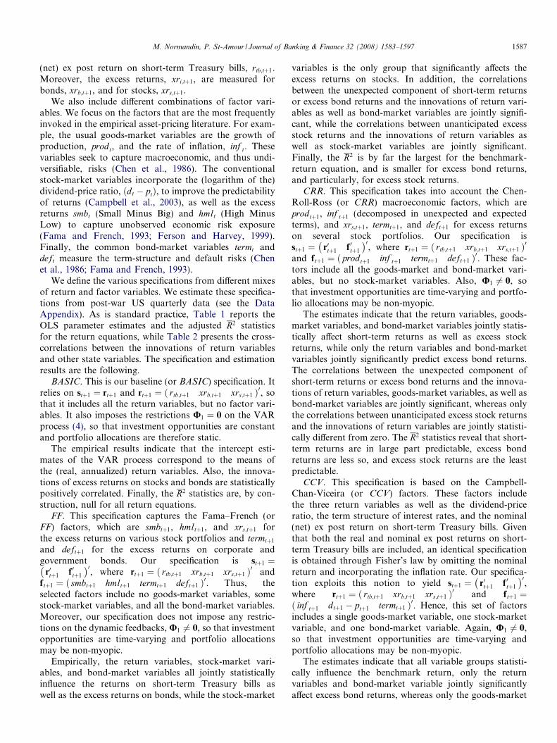
We also include different combinations of factor vari-ables. We focus on the factors that are the most frequentlyinvoked in the empirical asset-pricing literature. For exam-ple, the usual goods-market variables are the growth ofproduction, prodt, and the rate of inflation, inf t. Thesevariables seek to capture macroeconomic, and thus undi-versifiable, risks (Chen et al., 1986). The conventionalstock-market variables incorporate the (logarithm of the)dividend-price ratio, ðdt � ptÞ, to improve the predictabilityof returns (Campbell et al., 2003), as well as the excessreturns smbt (Small Minus Big) and hmlt (High MinusLow) to capture unobserved economic risk exposure(Fama and French, 1993; Ferson and Harvey, 1999).Finally, the common bond-market variables termt anddeft measure the term-structure and default risks (Chenet al., 1986; Fama and French, 1993).

We define the various specifications from different mixesof return and factor variables. We estimate these specifica-tions from post-war US quarterly data (see the DataAppendix). As is standard practice, Table 1 reports theOLS parameter estimates and the adjusted R2 statisticsfor the return equations, while Table 2 presents the cross-correlations between the innovations of return variablesand other state variables. The specification and estimationresults are the following.

BASIC. This is our baseline (or BASIC) specification. Itrelies on stþ1 ¼ rtþ1 and rtþ1 ¼ rtb;tþ1 xrb;tþ1 xrs;tþ1ð Þ0, sothat it includes all the return variables, but no factor vari-ables. It also imposes the restrictions U1 ¼ 0 on the VARprocess (4), so that investment opportunities are constantand portfolio allocations are therefore static.

The empirical results indicate that the intercept esti-mates of the VAR process correspond to the means ofthe (real, annualized) return variables. Also, the innova-tions of excess returns on stocks and bonds are statisticallypositively correlated. Finally, the R2 statistics are, by con-struction, null for all return equations.

FF. This specification captures the Fama–French (orFF) factors, which are smbtþ1, hmltþ1, and xrs;tþ1 forthe excess returns on various stock portfolios and termtþ1

and deftþ1 for the excess returns on corporate andgovernment bonds. Our specification is stþ1 ¼

r0tþ1 f 0tþ1

� �0, where rtþ1 ¼ rtb;tþ1 xrb;tþ1 xrs;tþ1ð Þ0 and

f tþ1 ¼ smbtþ1 hmltþ1 termtþ1 deftþ1ð Þ0. Thus, theselected factors include no goods-market variables, somestock-market variables, and all the bond-market variables.Moreover, our specification does not impose any restric-tions on the dynamic feedbacks, U1 6¼ 0, so that investmentopportunities are time-varying and portfolio allocationsmay be non-myopic.

Empirically, the return variables, stock-market vari-ables, and bond-market variables all jointly statisticallyinfluence the returns on short-term Treasury bills aswell as the excess returns on bonds, while the stock-market

variables is the only group that significantly affects theexcess returns on stocks. In addition, the correlationsbetween the unexpected component of short-term returnsor excess bond returns and the innovations of return vari-ables as well as bond-market variables are jointly signifi-cant, while the correlations between unanticipated excessstock returns and the innovations of return variables aswell as stock-market variables are jointly significant.Finally, the R2 is by far the largest for the benchmark-return equation, and is smaller for excess bond returns,and particularly, for excess stock returns.

CRR. This specification takes into account the Chen-Roll-Ross (or CRR) macroeconomic factors, which areprodtþ1, inf tþ1 (decomposed in unexpected and expectedterms), and xrs;tþ1, termtþ1, and deftþ1 for excess returnson several stock portfolios. Our specification isstþ1 ¼ r0tþ1 f 0tþ1

� �0, where rtþ1 ¼ rtb;tþ1 xrb;tþ1 xrs;tþ1ð Þ0

and f tþ1 ¼ prodtþ1 inf tþ1 termtþ1 deftþ1ð Þ0. These fac-tors include all the goods-market and bond-market vari-ables, but no stock-market variables. Also, U1 6¼ 0, sothat investment opportunities are time-varying and portfo-lio allocations may be non-myopic.

The estimates indicate that the return variables, goods-market variables, and bond-market variables jointly statis-tically affect short-term returns as well as excess stockreturns, while only the return variables and bond-marketvariables jointly significantly predict excess bond returns.The correlations between the unexpected component ofshort-term returns or excess bond returns and the innova-tions of return variables, goods-market variables, as well asbond-market variables are jointly significant, whereas onlythe correlations between unanticipated excess stock returnsand the innovations of return variables are jointly statisti-cally different from zero. The R2 statistics reveal that short-term returns are in large part predictable, excess bondreturns are less so, and excess stock returns are the leastpredictable.

CCV. This specification is based on the Campbell-Chan-Viceira (or CCV) factors. These factors includethe three return variables as well as the dividend-priceratio, the term structure of interest rates, and the nominal(net) ex post return on short-term Treasury bills. Giventhat both the real and nominal ex post returns on short-term Treasury bills are included, an identical specificationis obtained through Fisher’s law by omitting the nominalreturn and incorporating the inflation rate. Our specifica-tion exploits this notion to yield stþ1 ¼ r0tþ1 f 0tþ1

� �0,

where rtþ1 ¼ rtb;tþ1 xrb;tþ1 xrs;tþ1ð Þ0 and f tþ1 ¼inf tþ1 dtþ1 � ptþ1 termtþ1ð Þ0. Hence, this set of factors

includes a single goods-market variable, one stock-marketvariable, and one bond-market variable. Again, U1 6¼ 0,so that investment opportunities are time-varying andportfolio allocations may be non-myopic.

The estimates indicate that all variable groups statisti-cally influence the benchmark return, only the returnvariables and bond-market variable jointly significantlyaffect excess bond returns, whereas only the goods-market

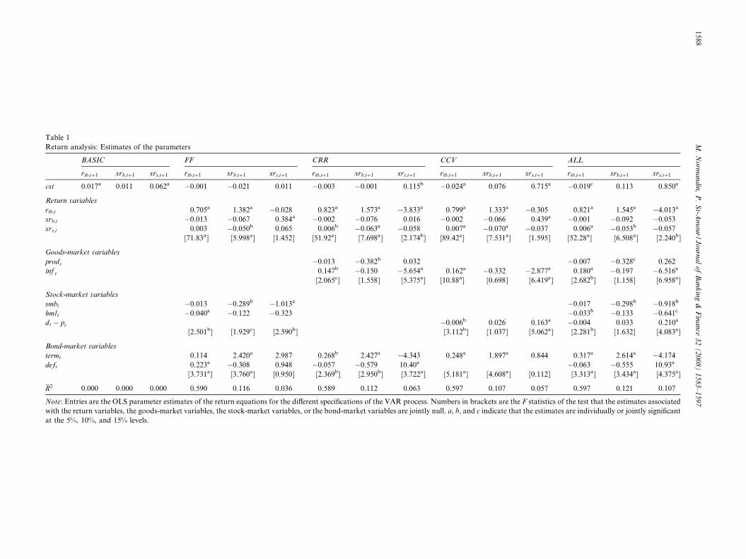
Table 1Return analysis: Estimates of the parameters

BASIC FF CRR CCV ALL

rtb;tþ1 xrb;tþ1 xrs;tþ1 rtb;tþ1 xrb;tþ1 xrs;tþ1 rtb;tþ1 xrb;tþ1 xrs;tþ1 rtb;tþ1 xrb;tþ1 xrs;tþ1 rtb;tþ1 xrb;tþ1 xrs;tþ1

cst 0.017a 0.011 0.062a �0.001 �0.021 0.011 �0.003 �0.001 0.115b �0.024a 0.076 0.715a �0.019c 0.113 0.850a

Return variables

rtb;t 0.705a 1.382a �0.028 0.823a 1.573a �3.833a 0.799a 1.333a �0.305 0.821a 1.545a �4.013a

xrb;t �0.013 �0.067 0.384a �0.002 �0.076 0.016 �0.002 �0.066 0.439a �0.001 �0.092 �0.053xrs;t 0.003 �0.050b 0.065 0.006b �0.063a �0.058 0.007a �0.070a �0.037 0.006a �0.053b �0.057

[71.83a] [5.998a] [1.452] [51.92a] [7.698a] [2.174b] [89.42a] [7.531a] [1.595] [52.28a] [6.508a] [2.240b]

Goods-market variables

prodt �0.013 �0.382b 0.032 �0.007 �0.328c 0.262inf t 0.147b �0.150 �5.654a 0.162a �0.332 �2.877a 0.180a �0.197 �6.516a

[2.065c] [1.558] [5.375a] [10.88a] [0.698] [6.419a] [2.682b] [1.158] [6.958a]

Stock-market variables

smbt �0.013 �0.289b �1.013a �0.017 �0.298b �0.918b

hmlt �0.040a �0.122 �0.323 �0.033b �0.133 �0.641c

dt � pt �0.006b 0.026 0.163a �0.004 0.033 0.210a

[2.501b] [1.929c] [2.590b] [3.112b] [1.037] [5.062a] [2.281b] [1.632] [4.083a]

Bond-market variables

termt 0.114 2.420a 2.987 0.268b 2.427a �4.343 0.248a 1.897a 0.844 0.317a 2.614a �4.174deft 0.223a �0.308 0.948 �0.057 �0.579 10.40a �0.063 �0.555 10.93a

[3.731a] [3.760a] [0.950] [2.369b] [2.950b] [3.722a] [5.181a] [4.608a] [0.112] [3.313a] [3.434a] [4.375a]

R2 0.000 0.000 0.000 0.590 0.116 0.036 0.589 0.112 0.063 0.597 0.107 0.057 0.597 0.121 0.107

Note: Entries are the OLS parameter estimates of the return equations for the different specifications of the VAR process. Numbers in brackets are the F statistics of the test that the estimates associatedwith the return variables, the goods-market variables, the stock-market variables, or the bond-market variables are jointly null. a, b, and c indicate that the estimates are individually or jointly significantat the 5%, 10%, and 15% levels.

1588M

.N

orm

an

din

,P

.S

t-Am

ou

r/J

ou

rna

lo

fB

an

kin

g&

Fin

an

ce3

2(

20

08

)1

58

3–

159

7

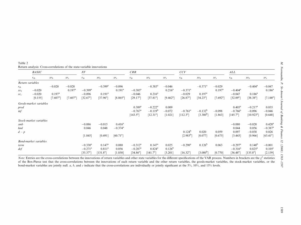
Table 2Return analysis: Cross-correlations of the state-variable innovations

BASIC FF CRR CCV ALL

rtb xrb xrs rtb xrb xrs rtb xrb xrs rtb xrb xrs rtb xrb xrs

Return variables

rtb �0.020 �0.020 �0.399a �0.096 �0.385a �0.046 �0.371a �0.029 �0.404a �0.047xrb �0.020 0.197a �0.399a 0.191a �0.385a 0.216a �0.371a 0.197a �0.404a 0.186a

xrs �0.020 0.197a �0.096 0.191a �0.046 0.216a �0.029 0.197a �0.047 0.186a

[0.155] [7.607a] [7.607a] [32.67a] [37.96a] [8.865a] [29.17a] [37.81a] [9.462a] [26.87a] [34.23a] [7.692a] [32.09a] [38.38a] [7.140a]


prod 0.389a �0.222a 0.009 0.405a �0.217a 0.035inf �0.767a �0.119b �0.072 �0.761a �0.132b �0.098 �0.766a �0.096 �0.046

[143.5a] [12.31a] [1.021] [112.3a] [3.380b] [1.863] [145.7a] [10.923a] [0.648]

Stock-market variables

smb �0.086 �0.015 0.416a �0.080 �0.020 0.420a

hml 0.046 0.048 �0.374a 0.044 0.056 �0.387a

d � p 0.124b 0.020 0.059 0.097 �0.038 0.026[1.845] [0.491] [60.71a] [2.983b] [0.077] [0.675] [3.443] [0.966] [63.41a]


term �0.330a 0.147a 0.080 �0.312a 0.147a 0.025 �0.290a 0.126b 0.063 �0.297a 0.140b �0.001def �0.271a 0.811a 0.056 �0.287a 0.824a 0.126b �0.316a 0.825a 0.105c

[35.37a] [131.8a] [1.850] [34.86a] [141.7a] [3.201] [16.32a] [3.080b] [0.770] [36.48a] [135.8a] [2.139]

Note: Entries are the cross-correlations between the innovations of return variables and other state variables for the different specifications of the VAR process. Numbers in brackets are the v2 statisticsof the Box-Pierce test that the cross-correlations between the innovations of each return variable and the other return variables, the goods-market variables, the stock-market variables, or thebond-market variables are jointly null. a, b, and c indicate that the cross-correlations are individually or jointly significant at the 5%, 10%, and 15% levels.

M.

No

rma

nd

in,

P.

St-A

mo

ur

/Jo

urn

al

of

Ba

nk

ing

&F

ina

nce

32

(2

00

8)

15

83

–1

59

71589


variable and stock-market variable statistically affect excessstock returns. The correlations between the unanticipatedbenchmark return and the innovations of all variablegroups are jointly statistically different from zero, the cor-relations between unexpected excess bond returns and theinnovations of return variables, goods-market variable,and bond-market variable are significant, while only thecorrelations between unanticipated excess stock returnsand the innovations of return variables are jointly signifi-cant. Again, the R2 is the largest for the benchmark-returnequation, is smaller for excess bond returns, and is thesmallest for excess stock returns.

ALL. This specification nests every (or ALL) factors ofthe previous specifications. That is, stþ1 ¼ r0tþ1 f 0tþ1

� �0,

where rtþ1 ¼ rtb;tþ1 xrb;tþ1 xrs;tþ1ð Þ0 and f tþ1 ¼prodtþ1 inf tþ1 smbtþ1 hmltþ1 dtþ1�ptþ1 termtþ1 deftþ1ð Þ0.

Thus, this set includes all the goods-market, stock-market,and bond-market variables. Furthermore, U1 6¼ 0.

Empirically, every variable group statistically affectsshort-term returns and excess stock returns, while onlythe return variables and bond-market variables jointly sig-nificantly alter excess bond returns. Moreover, the correla-tions between the unexpected benchmark return or excessbond returns and the innovations of return variables,goods-market variables, as well as bond-market variablesare jointly statistically different from zero, and the correla-tions between unexpected excess stock returns and theinnovations of return variables and stock-market variablesare jointly significant. Finally, the R2 statistics indicate thatshort-term returns are largely predictable, excess bondreturns are more difficult to forecast, and excess stockreturns are even more difficult to predict.

Overall, the return analysis reveals four important impli-cations for portfolio allocations. First, both the significancelevels of dynamic feedbacks and R2 statistics indicatethat the baseline specification is rejected. This findingrefutes the notion that investment opportunities areconstant, and thus, that portfolio allocations should bestatic. Second, the significance levels of dynamic feedbacksshow that certain variable groups affect the return variablesfor all alternative factor sets. This result accords with the

Table 3Portfolio analysis: Empirical shares

Mean Volatility

cash bond stock cash bond

OfficialData 0.458 0.092 0.450 0.122 0.034

AdjustedData1 year 0.460 0.088 0.452 0.123 0.0343 years 0.465 0.079 0.456 0.125 0.0345 years 0.469 0.071 0.460 0.126 0.03410 years 0.477 0.055 0.468 0.128 0.03220 years 0.479 0.035 0.479 0.128 0.027

Note: OfficialData: Entries are the means, standard deviations, and cross-corstocks computed from official data. These data record the market values of cameans, standard deviations, and cross-correlations of the empirical householdThese data approximate the market values of bonds under the assumptions tha

empirical asset-pricing literature documenting the predict-ability of returns, and confirms that investment opportuni-ties are time-varying. Third, the significance levels ofinnovation correlations highlight several co-movementsbetween the return and factor variables. These co-move-ments are necessary conditions for dynamic hedging strat-egies, which accords with the fact that the empirical sharesof cash, bonds, and stocks feature pronounced fluctuationsthrough time (see Figs. 1 and 2). Fourth, the R2 statisticsare very close across the various alternative factor sets.Consequently, the identification of the most influential fac-tor set for portfolio allocations remains an open question.For this reason, rather than focusing on a single factorialspecification, we next perform our portfolio analysis forevery factor sets.

4. Portfolio analysis

This section compares the empirical and predictedhousehold portfolio shares. For this purpose, the empiricalshares are constructed for cash, bonds, and stocks by eval-uating the definition (6) from a measure of (financial)wealth corresponding to the sum of the aggregate valuesof the three assets hold by households and from quarterlyUS data covering the post-war period (see the Data Appen-dix). In comparison, the values of cash, treasury securities,corporate equity, and total financial assets directly held byhouseholds in 2005 correspond to 64.1%, 11.7%, 30.0%,and 32.9% of those for all sectors, which also include busi-nesses, governments, and non-residents (Source: Board ofGovernors of the Federal Reserve Bank, Balance Sheet ofAll Sectors).

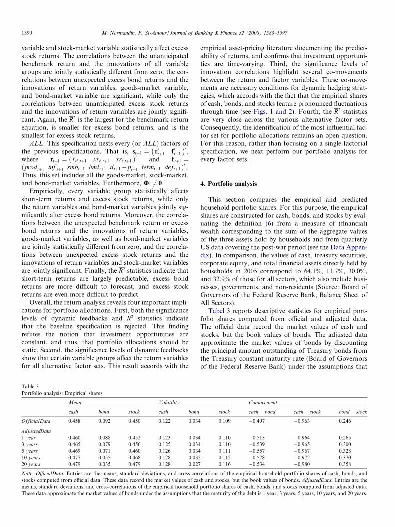
Tabel 3 reports descriptive statistics for empirical port-folio shares computed from official and adjusted data.The official data record the market values of cash andstocks, but the book values of bonds. The adjusted dataapproximate the market values of bonds by discountingthe principal amount outstanding of Treasury bonds fromthe Treasury constant maturity rate (Board of Governorsof the Federal Reserve Bank) under the assumptions that

Comovement

stock cash� bond cash� stock bond � stock

0.109 �0.497 �0.963 0.246

0.110 �0.513 �0.964 0.2650.110 �0.539 �0.965 0.3000.111 �0.557 �0.967 0.3280.112 �0.578 �0.972 0.3700.116 �0.534 �0.980 0.358

relations of the empirical household portfolio shares of cash, bonds, andsh and stocks, but the book values of bonds. AdjustedData: Entries are theportfolio shares of cash, bonds, and stocks computed from adjusted data.t the maturity of the debt is 1 year, 3 years, 5 years, 10 years, and 20 years.


the maturity of the debt is 1 year, 3 years, 5 years, 10 years,and 20 years.

Importantly, the empirical portfolio shares computedfrom official and adjusted data exhibit similar features. Inparticular, both the empirical shares of cash and stocks dis-play large means and volatilities, whereas the empiricalshare of bonds has much lower average and standard devi-ation. Also, the empirical share of cash exhibits negativeco-movements with the empirical share of bonds as wellas the one for stocks, while the empirical shares of bondsand stocks are positively correlated. Given the robustnessof the results, the remaining of the paper uses the empiricalportfolio shares computed from official data.

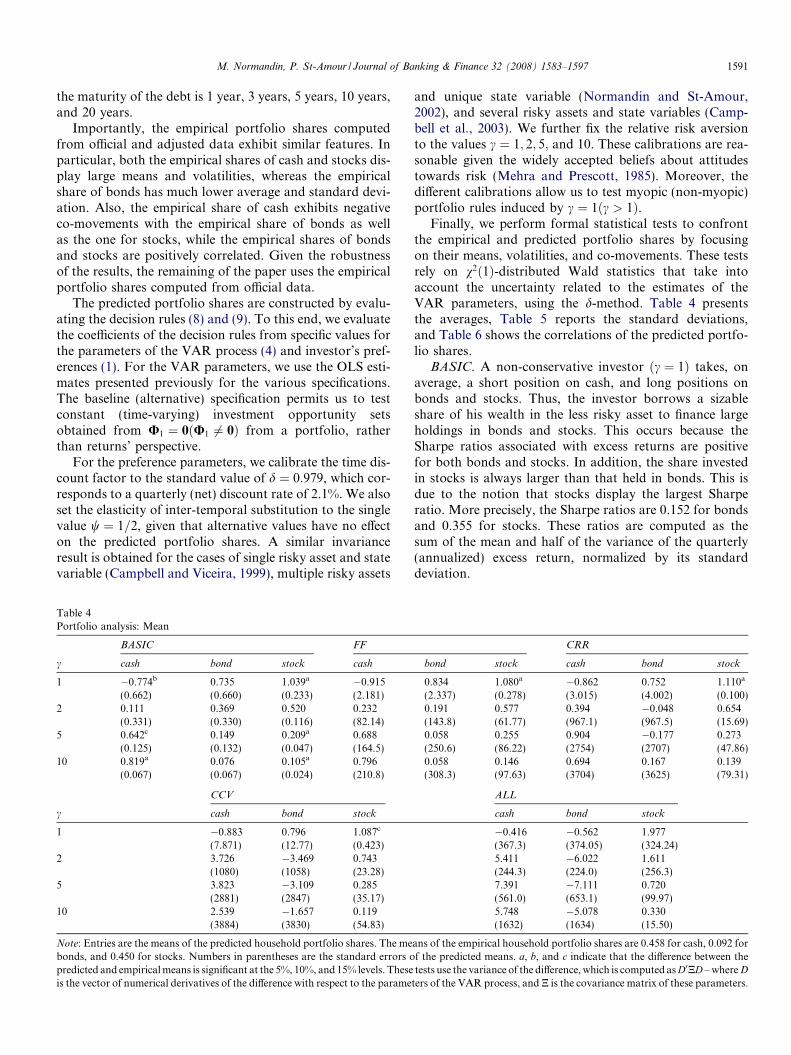
The predicted portfolio shares are constructed by evalu-ating the decision rules (8) and (9). To this end, we evaluatethe coefficients of the decision rules from specific values forthe parameters of the VAR process (4) and investor’s pref-erences (1). For the VAR parameters, we use the OLS esti-mates presented previously for the various specifications.The baseline (alternative) specification permits us to testconstant (time-varying) investment opportunity setsobtained from U1 ¼ 0ðU1 6¼ 0Þ from a portfolio, ratherthan returns’ perspective.

For the preference parameters, we calibrate the time dis-count factor to the standard value of d ¼ 0:979, which cor-responds to a quarterly (net) discount rate of 2.1%. We alsoset the elasticity of inter-temporal substitution to the singlevalue w ¼ 1=2, given that alternative values have no effecton the predicted portfolio shares. A similar invarianceresult is obtained for the cases of single risky asset and statevariable (Campbell and Viceira, 1999), multiple risky assets

Table 4Portfolio analysis: Mean

BASIC FF

c cash bond stock cash

1 �0.774b 0.735 1.039a �0.915(0.662) (0.660) (0.233) (2.181)

2 0.111 0.369 0.520 0.232(0.331) (0.330) (0.116) (82.14)

5 0.642c 0.149 0.209a 0.688(0.125) (0.132) (0.047) (164.5)

10 0.819a 0.076 0.105a 0.796(0.067) (0.067) (0.024) (210.8)

CCV

c cash bond stock

1 �0.883 0.796 1.087c

(7.871) (12.77) (0.423)2 3.726 �3.469 0.743

(1080) (1058) (23.28)5 3.823 �3.109 0.285

(2881) (2847) (35.17)10 2.539 �1.657 0.119

(3884) (3830) (54.83)

Note: Entries are the means of the predicted household portfolio shares. The mebonds, and 0.450 for stocks. Numbers in parentheses are the standard errors opredicted and empirical means is significant at the 5%, 10%, and 15% levels. Theseis the vector of numerical derivatives of the difference with respect to the parame

and unique state variable (Normandin and St-Amour,2002), and several risky assets and state variables (Camp-bell et al., 2003). We further fix the relative risk aversionto the values c ¼ 1; 2; 5; and 10. These calibrations are rea-sonable given the widely accepted beliefs about attitudestowards risk (Mehra and Prescott, 1985). Moreover, thedifferent calibrations allow us to test myopic (non-myopic)portfolio rules induced by c ¼ 1ðc > 1Þ.

Finally, we perform formal statistical tests to confrontthe empirical and predicted portfolio shares by focusingon their means, volatilities, and co-movements. These testsrely on v2ð1Þ-distributed Wald statistics that take intoaccount the uncertainty related to the estimates of theVAR parameters, using the d-method. Table 4 presentsthe averages, Table 5 reports the standard deviations,and Table 6 shows the correlations of the predicted portfo-lio shares.

BASIC. A non-conservative investor ðc ¼ 1Þ takes, onaverage, a short position on cash, and long positions onbonds and stocks. Thus, the investor borrows a sizableshare of his wealth in the less risky asset to finance largeholdings in bonds and stocks. This occurs because theSharpe ratios associated with excess returns are positivefor both bonds and stocks. In addition, the share investedin stocks is always larger than that held in bonds. This isdue to the notion that stocks display the largest Sharperatio. More precisely, the Sharpe ratios are 0.152 for bondsand 0.355 for stocks. These ratios are computed as thesum of the mean and half of the variance of the quarterly(annualized) excess return, normalized by its standarddeviation.

CRR

bond stock cash bond stock

0.834 1.080a �0.862 0.752 1.110a

(2.337) (0.278) (3.015) (4.002) (0.100)0.191 0.577 0.394 �0.048 0.654(143.8) (61.77) (967.1) (967.5) (15.69)0.058 0.255 0.904 �0.177 0.273(250.6) (86.22) (2754) (2707) (47.86)0.058 0.146 0.694 0.167 0.139(308.3) (97.63) (3704) (3625) (79.31)

ALL

cash bond stock

�0.416 �0.562 1.977(367.3) (374.05) (324.24)5.411 �6.022 1.611(244.3) (224.0) (256.3)7.391 �7.111 0.720(561.0) (653.1) (99.97)5.748 �5.078 0.330(1632) (1634) (15.50)

ans of the empirical household portfolio shares are 0.458 for cash, 0.092 forf the predicted means. a, b, and c indicate that the difference between thetests use the variance of the difference, which is computed as D0ND – where D

ters of the VAR process, and N is the covariance matrix of these parameters.

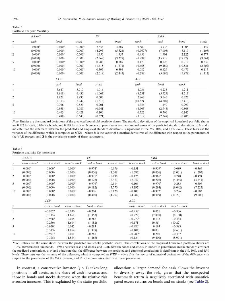
Table 5Portfolio analysis: Volatility

BASIC FF CRR

c cash bond stock cash bond stock cash bond stock

1 0.000a 0.000a 0.000a 3.856 3.889 0.880 3.736 4.005 1.147(0.000) (0.000) (0.000) (4.293) (5.524) (0.9677) (7.003) (8.110) (1.108)

2 0.000a 0.000a 0.000a 1.950 1.955 0.436 1.904 2.122 0.577(0.000) (0.000) (0.000) (2.368) (3.229) (0.834) (15.81) (17.27) (3.661)

5 0.000a 0.000a 0.000a 0.788 0.787 0.173 0.826 0.919 0.232(0.000) (0.000) (0.000) (1.615) (1.871) (0.465) (9.180) (10.53) (2.307)

10 0.000a 0.000a 0.000a 0.395 0.394 0.087 0.429 0.475 0.117(0.000) (0.000) (0.000) (2.519) (2.443) (0.288) (5.095) (5.978) (1.313)

CCV ALL

c cash bond stock cash bond stock

1 3.647 3.717 1.016 4.036 4.238 1.211(4.918) (6.435) (1.063) (8.231) (5.727) (4.213)

2 1.921 1.993 0.503 2.862 3.045 0.726(2.313) (2.747) (1.618) (10.62) (4.207) (2.413)

5 0.796 0.829 0.201 1.356 1.440 0.290(0.958) (1.080) (0.941) (4.903) (2.745) (0.808)

10 0.403 0.421 0.100 0.723 0.766 0.145(0.498) (0.543) (0.521) (3.012) (2.249) (0.405)

Note: Entries are the standard deviations of the predicted household portfolio shares. The standard deviations of the empirical household portfolio sharesare 0.122 for cash, 0.034 for bonds, and 0.109 for stocks. Numbers in parentheses are the standard errors of the predicted standard deviations. a, b, and c

indicate that the difference between the predicted and empirical standard deviations is significant at the 5%, 10%, and 15% levels. These tests use thevariance of the difference, which is computed as D0ND – where D is the vector of numerical derivatives of the difference with respect to the parameters ofthe VAR process, and N is the covariance matrix of these parameters.

Table 6Portfolio analysis: Co-movement

BASIC FF CRR

c cash� bond cash� stock bond � stock cash� bond cash� stock bond � stock cash� bond cash� stock bond � stock

1 0.000a 0.000a 0.000a �0.974a �0.076 �0.151 �0.959a 0.089 �0.369(0.000) (0.000) (0.000) (0.056) (1.508) (1.387) (0.056) (2.001) (1.203)

2 0.000a 0.000a 0.000a �0.975a �0.098 �0.125 �0.965a 0.248 �0.494(0.000) (0.000) (0.000) (0.123) (2.473) (2.059) (0.206) (4.465) (3.641)

5 0.000a 0.000a 0.000a �0.976a �0.114 �0.106 �0.970b 0.283 �0.507(0.000) (0.000) (0.000) (0.182) (3.770) (3.192) (0.284) (9.042) (7.223)

10 0.000a 0.000a 0.000a �0.976 �0.120 �0.100 �0.972c 0.286 �0.503(0.000) (0.000) (0.000) (0.410) (4.252) (4.289) (0.319) (11.20) (9.000)

CCV ALL

c cash� bond cash� stock bond � stock cash� bond cash� stock bond � stock

1 �0.962a �0.070 �0.204 �0.958a 0.021 �0.306(0.115) (1.661) (1.353) (0.229) (7.898) (8.180)

2 �0.968a 0.015 �0.267 �0.972a 0.133 �0.364(0.230) (1.614) (1.182) (0.171) (10.35) (10.22)

5 �0.970c 0.042 �0.283 �0.980a 0.193 �0.383(0.313) (1.854) (1.378) (0.104) (10.03) (9.601)

10 �0.971c 0.051 �0.287 �0.983a 0.210 �0.387(0.325) (1.884) (1.466) (0.124) (9.400) (8.991)

Note: Entries are the correlations between the predicted household portfolio shares. The correlations of the empirical household portfolio shares are�0.497 between cash and bonds, �0.963 between cash and stocks, and 0.246 between bonds and stocks. Numbers in parentheses are the standard errors ofthe predicted correlations. a, b, and c indicate that the difference between the predicted and empirical correlations is significant at the 5%, 10%, and 15%levels. These tests use the variance of the difference, which is computed as D0ND – where D is the vector of numerical derivatives of the difference withrespect to the parameters of the VAR process, and N is the covariance matrix of these parameters.


In contrast, a conservative investor ðc > 1Þ takes longpositions in all assets, as the share of cash increases andthose in bonds and stocks decrease when the relative riskaversion increases. This is explained by the static portfolio

allocation: a larger demand for cash allows the investorto diversify away the risk, given that the unexpectedbenchmark return is negatively correlated with unantici-pated excess returns on bonds and on stocks (see Table 2).


However, there is no such increase in the demand forbonds, since unanticipated excess returns on bonds andstocks are positively correlated.

For almost all reasonable values of relative risk aver-sion, the averages of the predicted portfolio shares of cashand stocks are significantly different from those of theempirical shares. Furthermore, the zero standard devia-tions and correlations of the predicted shares are alwaysstatistically different from their empirical counterparts. Insum, these test results indicate that the investor’s staticbehavior is rejected by the data.

FF. A myopic investor ðc ¼ 1Þ takes, on average, a shortposition on cash, and long positions on bonds and stocks.This myopic behavior is similar than the static behaviorjust explained for the BASIC case. This arises because boththe myopic and static portfolio allocations abstract fromhedging strategies.

From a statistical perspective, the myopic behavior pre-dicts a mean for the share of stocks and a correlationbetween the shares of cash and bonds that are significantlydifferent from their empirical counterparts. In addition, allthe means (in absolute values) and volatilities, as well asmost correlations (in absolute values) of the predictedshares largely numerically over-state those of the empiricalshares. These findings are not in favor of the myopicbehavior.

A non-myopic investor ðc > 1Þ takes long positions inall assets, as the share of cash increases and those in bondsand stocks decrease when the relative risk aversionincreases. Interestingly, the non-myopic behavior impliesthat the decrease in the share of stocks (bonds) is less(more) pronounced, relative to that found from the staticbehavior. This suggests that stocks are better dynamichedges against adverse changes in investment oppor-tunities.

Statistically, the non-myopic behavior predicts meansand volatilities that are never significantly different fromthose found in the data. This behavior further predicts cor-relations for the shares of cash and bonds with that ofstocks that are never statistically different from the empir-ical ones, whereas most of the predicted correlationsbetween the shares of cash and bonds are significantly dif-ferent from the data. Admittedly, most of these inferenceresults reflect the fact that the predicted portfolio sharesare very imprecisely estimated. As a result, the confidenceintervals around the point estimates of the variousmoments are very large, and as such typically include thevalues of the moments computed from the empirical port-folio shares. This inefficiency problem is especially impor-tant when the investment opportunity set is time variant.Also, this problem becomes even more severe as the riskaversion increases.

Nevertheless, it is worth stressing that the predictedshares exhibit the appropriate signs and magnitudes forthe means when c ¼ 2 and 5 for all assets, and adequatevolatilities when c ¼ 5 and 10 for stocks. In addition, thepredicted correlations for the share of cash with those of

bonds and stocks display the correct signs, regardless ofthe value of c. Overall, these results provide empirical sup-port for the non-myopic portfolio allocation obtained bycombining reasonable degrees of risk aversions with theFF set of factors.

CRR. As above, a myopic investor ðc ¼ 1Þ takes, onaverage, a short position on cash, and long positions onbonds and stocks. Also, the predicted mean for the shareof stocks and correlation between the shares of cash andbonds are statistically at odds with the data. Finally, allthe predicted means (in absolute values) and volatilitiesover-estimate the empirical ones, while the predicted corre-lations often display the wrong signs. Again, these findingsindicate that the myopic behavior is refuted.

A non-myopic investor ðc > 1Þ usually takes long posi-tions in cash and stocks, but short positions in bonds. Also,the non-myopic behavior induced by the CRR factor setimplies that the fall in demand for bonds is so pronouncedthat it drives the share of bonds to be negative, in contrastto that obtained from the FF case.

The test results reveal that the non-myopic behaviorassociated with the CRR specification predicts means andvolatilities that are never statistically different from theempirical ones. Also, the predicted correlations for theshares of cash and bonds with that of stocks are never sta-tistically different from the empirical ones, whereas the pre-dicted correlations between the shares of cash and bondsare significantly different from the data. Again, most ofthese inference results reflect the fact that the predictedportfolio shares are very imprecisely estimated.

However, the predicted means for the share of bonds isalmost always negative, whereas the empirical counterpartis positive. Moreover, the correlations between the sharesof cash and stocks exhibit the wrong sign, for almost allreasonable values of c. For these reasons, the non-myopicportfolio allocation derived from the CRR specificationis performing worse than the one related to the FF factorset.

CCV. A myopic investor ðc ¼ 1Þ takes, on average, iden-tical asset positions as those explained previously. Also,this myopic behavior features similar statistical and numer-ical properties as those described above. Consequently, themyopic behavior is once again inconsistent with the data.

A non-myopic investor ðc > 1Þ takes similar asset posi-tions as those explained for the CRR specification. How-ever, the predicted means for the portfolio shares seemeconomically rather implausible, as they over-state theempirical ones by a large order of magnitude. Moreover,the predicted means for the share of bonds and correlationsbetween the shares of cash and stocks systematically dis-play the wrong signs. Hence, the non-myopic portfolioallocation derived from the CCV specification is also lessattractive than the one associated with the FF factor set.

ALL. A myopic investor ðc ¼ 1Þ is characterized by abehavior that is numerically and statistically close to thatdocumented above. As a result, the myopic behavior isonce more time at odds with the data.

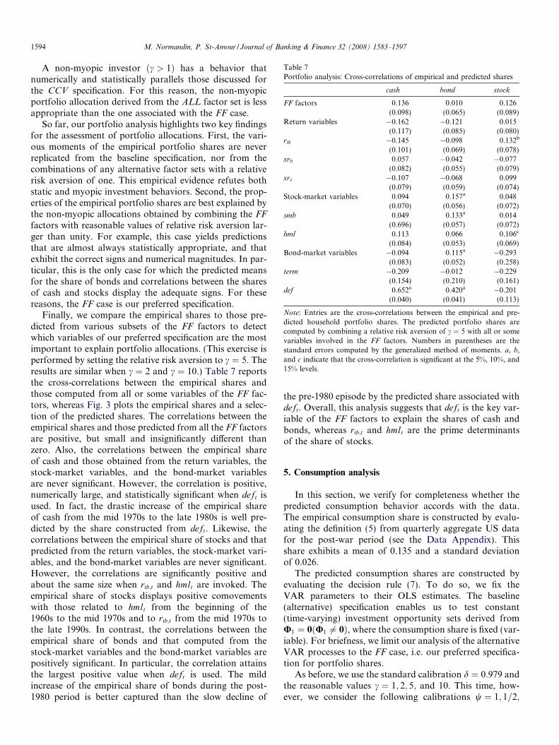
Table 7Portfolio analysis: Cross-correlations of empirical and predicted shares

cash bond stock

FF factors 0.136 0.010 0.126(0.098) (0.065) (0.089)

Return variables �0.162 �0.121 0.015(0.117) (0.085) (0.080)

rtb �0.145 �0.098 0.132b

(0.101) (0.069) (0.078)xrb 0.057 �0.042 �0.077

(0.082) (0.055) (0.079)xrs �0.107 �0.068 0.099

(0.079) (0.059) (0.074)Stock-market variables 0.094 0.157a 0.048

(0.070) (0.056) (0.072)smb 0.049 0.133a 0.014

(0.696) (0.057) (0.072)hml 0.113 0.066 0.106c

(0.084) (0.053) (0.069)Bond-market variables �0.094 0.115a �0.293

(0.083) (0.052) (0.258)term �0.209 �0.012 �0.229

(0.154) (0.210) (0.161)def 0.652a 0.420a �0.201

(0.040) (0.041) (0.113)

Note: Entries are the cross-correlations between the empirical and pre-dicted household portfolio shares. The predicted portfolio shares arecomputed by combining a relative risk aversion of c ¼ 5 with all or somevariables involved in the FF factors. Numbers in parentheses are thestandard errors computed by the generalized method of moments. a, b,and c indicate that the cross-correlation is significant at the 5%, 10%, and15% levels.


A non-myopic investor ðc > 1Þ has a behavior thatnumerically and statistically parallels those discussed forthe CCV specification. For this reason, the non-myopicportfolio allocation derived from the ALL factor set is lessappropriate than the one associated with the FF case.

So far, our portfolio analysis highlights two key findingsfor the assessment of portfolio allocations. First, the vari-ous moments of the empirical portfolio shares are neverreplicated from the baseline specification, nor from thecombinations of any alternative factor sets with a relativerisk aversion of one. This empirical evidence refutes bothstatic and myopic investment behaviors. Second, the prop-erties of the empirical portfolio shares are best explained bythe non-myopic allocations obtained by combining the FFfactors with reasonable values of relative risk aversion lar-ger than unity. For example, this case yields predictionsthat are almost always statistically appropriate, and thatexhibit the correct signs and numerical magnitudes. In par-ticular, this is the only case for which the predicted meansfor the share of bonds and correlations between the sharesof cash and stocks display the adequate signs. For thesereasons, the FF case is our preferred specification.

Finally, we compare the empirical shares to those pre-dicted from various subsets of the FF factors to detectwhich variables of our preferred specification are the mostimportant to explain portfolio allocations. (This exercise isperformed by setting the relative risk aversion to c ¼ 5. Theresults are similar when c ¼ 2 and c ¼ 10.) Table 7 reportsthe cross-correlations between the empirical shares andthose computed from all or some variables of the FF fac-tors, whereas Fig. 3 plots the empirical shares and a selec-tion of the predicted shares. The correlations between theempirical shares and those predicted from all the FF factorsare positive, but small and insignificantly different thanzero. Also, the correlations between the empirical shareof cash and those obtained from the return variables, thestock-market variables, and the bond-market variablesare never significant. However, the correlation is positive,numerically large, and statistically significant when deft isused. In fact, the drastic increase of the empirical shareof cash from the mid 1970s to the late 1980s is well pre-dicted by the share constructed from deft. Likewise, thecorrelations between the empirical share of stocks and thatpredicted from the return variables, the stock-market vari-ables, and the bond-market variables are never significant.However, the correlations are significantly positive andabout the same size when rtb;t and hmlt are invoked. Theempirical share of stocks displays positive comovementswith those related to hmlt from the beginning of the1960s to the mid 1970s and to rtb;t from the mid 1970s tothe late 1990s. In contrast, the correlations between theempirical share of bonds and that computed from thestock-market variables and the bond-market variables arepositively significant. In particular, the correlation attainsthe largest positive value when deft is used. The mildincrease of the empirical share of bonds during the post-1980 period is better captured than the slow decline of

the pre-1980 episode by the predicted share associated withdeft. Overall, this analysis suggests that deft is the key var-iable of the FF factors to explain the shares of cash andbonds, whereas rtb;t and hmlt are the prime determinantsof the share of stocks.

5. Consumption analysis

In this section, we verify for completeness whether thepredicted consumption behavior accords with the data.The empirical consumption share is constructed by evalu-ating the definition (5) from quarterly aggregate US datafor the post-war period (see the Data Appendix). Thisshare exhibits a mean of 0.135 and a standard deviationof 0.026.

The predicted consumption shares are constructed byevaluating the decision rule (7). To do so, we fix theVAR parameters to their OLS estimates. The baseline(alternative) specification enables us to test constant(time-varying) investment opportunity sets derived fromU1 ¼ 0ðU1 6¼ 0Þ, where the consumption share is fixed (var-iable). For briefness, we limit our analysis of the alternativeVAR processes to the FF case, i.e. our preferred specifica-tion for portfolio shares.

As before, we use the standard calibration d ¼ 0:979 andthe reasonable values c ¼ 1; 2; 5; and 10. This time, how-ever, we consider the following calibrations w ¼ 1; 1=2;

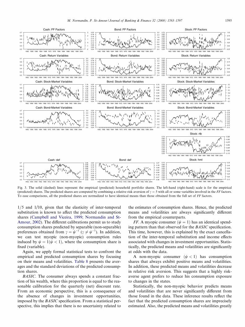
Fig. 3. The solid (dashed) lines represent the empirical (predicted) household portfolio shares. The left-hand (right-hand) scale is for the empirical(predicted) shares. The predicted shares are computed by combining a relative risk aversion of c ¼ 5 with all or some variables involved in the FF factors.To ease comparisons, all the predicted shares are normalized to have identical means than those obtained from the full set of FF factors.


1=5 and 1/10, given that the elasticity of inter-temporalsubstitution is known to affect the predicted consumptionshares (Campbell and Viceira, 1999; Normandin and St-Amour, 2002). The different calibrations permit us to studyconsumption shares predicted by separable (non-separable)preferences obtained from c ¼ w�1 (c 6¼ w�1). In addition,we can test myopic (non-myopic) consumption rulesinduced by w ¼ 1ðw < 1Þ, where the consumption share isfixed (variable).

Again, we apply formal statistical tests to confront theempirical and predicted consumption shares by focusingon their means and volatilities. Table 8 presents the aver-ages and the standard deviations of the predicted consump-tion shares.

BASIC. The consumer always spends a constant frac-tion of his wealth, where this proportion is equal to the rea-sonable calibration for the quarterly (net) discount rate.From an economic perspective, this is a consequence ofthe absence of changes in investment opportunities,imposed by the BASIC specification. From a statistical per-spective, this implies that there is no uncertainty related to

the estimates of consumption shares. Hence, the predictedmeans and volatilities are always significantly differentfrom the empirical counterparts.

FF. A myopic consumer ðw ¼ 1Þ has an identical spend-ing pattern than that observed for the BASIC specification.This time, however, this is explained by the exact cancella-tion of the inter-temporal substitution and income effectsassociated with changes in investment opportunities. Statis-tically, the predicted means and volatilities are significantlyat odds with the data.

A non-myopic consumer ðw < 1Þ has consumptionshares that always exhibit positive means and volatilities.In addition, these predicted means and volatilities decreasein relative risk aversion. This suggests that a highly risk-averse agent prefers to reduce his consumption exposureto changes in the states.

Statistically, the non-myopic behavior predicts meansand volatilities that are never significantly different fromthose found in the data. These inference results reflect thefact that the predicted consumption shares are impreciselyestimated. Also, the predicted means and volatilities greatly

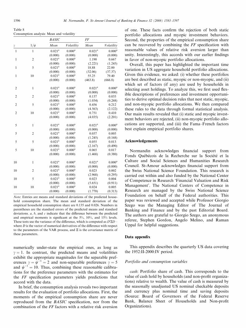
Table 8Consumption analysis: Mean and volatility

BASIC FF

c 1=w Mean Volatility Mean Volatility

1 1 0.021a 0.000a 0.021a 0.000a

(0.000) (0.000) (0.000) (0.000)1 2 0.021a 0.000a 1.190 0.667

(0.000) (0.000) (2.221) (1.245)1 5 0.021a 0.000a 18.88 22.00

(0.000) (0.000) (32.06) (37.37)1 10 0.021a 0.000a 55.25 79.40

(0.000) (0.000) (463.8) (666.8)

2 1 0.021a 0.000a 0.021a 0.000a

(0.000) (0.000) (0.000) (0.000)2 2 0.021a 0.000a 0.137 0.035

(0.000) (0.000) (1.034) (0.268)2 5 0.021a 0.000a 0.456 0.212

(0.000) (0.000) (4.563) (2.122)2 10 0.021a 0.000a 0.751 0.410

(0.000) (0.000) (4.035) (2.201)

5 1 0.021a 0.000a 0.021a 0.000a

(0.000) (0.000) (0.000) (0.000)5 2 0.021a 0.000a 0.037 0.005

(0.000) (0.000) (1.245) (0.168)5 5 0.021a 0.000a 0.055 0.013

(0.000) (0.000) (2.167) (0.490)5 10 0.021a 0.000a 0.065 0.017

(0.000) (0.000) (1.468) (0.380)

10 1 0.021a 0.000a 0.021a 0.000a

(0.000) (0.000) (0.000) (0.000)10 2 0.021a 0.000a 0.023 0.002

(0.000) (0.000) (2.968) (0.295)10 5 0.021a 0.000a 0.023 0.004

(0.000) (0.000) (5.651) (0.911)10 10 0.021a 0.000a 0.024 0.005

(0.000) (0.000) (1.770) (0.313)

Note: Entries are means and standard deviations of the predicted house-hold consumption share. The mean and standard deviation of theempirical household consumption share are 0.135 and 0.026. Numbers inparentheses are the standard errors of the predicted means and standarddeviations. a, b, and c indicate that the difference between the predictedand empirical moments is significant at the 5%, 10%, and 15% levels.These tests use the variance of the difference, which is computed as D0ND –where D is the vector of numerical derivatives of the difference with respectto the parameters of the VAR process, and N is the covariance matrix ofthese parameters.


numerically under-state the empirical ones, as long asc ¼ 1. In contrast, the predicted means and volatilitiesexhibit the appropriate magnitudes for the separable pref-erences c ¼ w�1 ¼ 2 and non-separable preferences c ¼ 5and w�1 ¼ 10. Thus, combining these reasonable calibra-tions for the preference parameters with the estimates forthe FF specification parameters yields predictions thataccord with the data.

In brief, the consumption analysis reveals two importantresults for the evaluation of portfolio allocations. First, themoments of the empirical consumption share are neverreproduced from the BASIC specification, nor from thecombination of the FF factors with a relative risk aversion

of one. These facts confirm the rejection of both staticportfolio allocations and myopic investment behaviors.Second, the properties of the empirical consumption sharecan be recovered by combining the FF specification withreasonable values of relative risk aversion larger thanunity. Interestingly, this accords with our earlier findingsin favor of non-myopic portfolio allocations.

Overall, this paper has highlighted the important timevariation in US aggregate household portfolio allocations.Given this evidence, we asked: (i) whether these portfoliosare best described as static, myopic or non-myopic, and (ii)which set of factors (if any) are used by households inselecting asset holdings. To analyze this, we first used flex-ible descriptions of preferences and investment opportuni-ties to derive optimal decision rules that nest static, myopic,and non-myopic portfolio allocations. We then comparedthese rules to the data through formal statistical analysis.Our main results revealed that (i) static and myopic invest-ment behaviors are rejected, (ii) non-myopic portfolio allo-cations are supported, and (iii) the Fama–French factorsbest explain empirical portfolio shares.

Acknowledgements

Normandin acknowledges financial support fromFonds Quebecois de la Recherche sur la Societe et laCulture and Social Sciences and Humanities ResearchCouncil. St-Amour acknowledges financial support fromthe Swiss National Science Foundation. This research iscarried out within and also funded by the National Centerof Competence in Research ‘Financial Valuation and RiskManagement’. The National Centers of Competence inResearch are managed by the Swiss National ScienceFoundation on behalf of the Federal authorities. Thispaper was reviewed and accepted while Professor GiorgioSzego was the Managing Editor of The Journal ofBanking and Finance and by the past Editorial Board.The authors are grateful to Giorgio Szego, an anonymousreferee, Stephen Gordon, Angelo Melino, and RamanUppal for helpful suggestions.

Data appendix

This appendix describes the quarterly US data coveringthe 1952:II-2000:IV period.

Portfolio and consumption variables

cash: Portfolio share of cash. This corresponds to thevalue of cash hold by households (and non-profit organiza-tions) relative to wealth. The value of cash is measured bythe seasonally unadjusted US nominal checkable depositsand currency plus nominal time and saving deposits(Source: Board of Governors of the Federal ReserveBank, Balance Sheet of Households and Non-profitOrganizations).


bond: portfolio share of bonds. This is the value ofbonds hold by households (and non-profit organizations)divided by wealth. The value of bonds is captured by theseasonally unadjusted nominal US government securities(Source: Board of Governors of the Federal Reserve Bank,Balance Sheet of Households and Non-profit Organi-zations).

stock: portfolio share of stocks. This is the value ofstocks hold by households (and non-profit organizations)normalized by wealth. The value of stocks corresponds tothe seasonally unadjusted US nominal corporate equities(Source: Board of Governors of the Federal Reserve Bank,Balance Sheet of Households and Non-profit Organi-zations).

cons: consumption share. This is the value of consump-tion of households divided by wealth. The value of con-sumption is measured by the seasonally adjusted USnominal private consumption expenditures on non-durablegoods and services (Source: US Department of Commerce,Bureau of Economic Analysis).

wealth. This is the sum of the values of cash, bonds, andstocks.

Return variables

rtb;t: Ex post real Treasury bill rate. This is the differencebetween the quarterly (annualized) nominal return on 90-day US Treasury bill (Source: Center for Research in Secu-rity Prices) and the inflation rate.

xrb;t: excess bond return. This is the difference betweenthe quarterly (annualized) nominal return on five-yearUS Treasury bonds (Source: Center for Research in Secu-rity Prices) and the quarterly (annualized) nominal returnon 90-day US Treasury bill.

xrs;t: excess stock return. This is the difference betweenthe quarterly (annualized) nominal value-weighted return(including dividends) on the NYSE, NASDAQ, andAMEX markets (Source: Center for Research in SecurityPrices) and the quarterly (annualized) nominal return on90-day US Treasury bill.


inf t: Inflation rate. This is the quarterly (annualized)growth rate of the seasonally adjusted US gross domesticproduct implicit deflator (Source: US Department of Com-merce, Bureau of Economic Analysis).

prodt: production growth. This is the difference betweenthe quarterly (annualized) growth rate of the seasonallyadjusted US nominal gross domestic product (Source: USDepartment of Commerce, Bureau of Economic Analysis)and the inflation rate.

Equity-market variables

smbt (Small Minus Big): Excess small-portfolio return.This is the difference between the quarterly (annualized)

average return on three small US portfolios and thequarterly (annualized) average return on three big USportfolios (Source: http://mba.tuck.dartmouth.edu/pages/faculty/ken.french/data_library.html).

hmlt (High Minus Low): excess value-portfolio return.This is the difference between the quarterly (annualized)average return on two value US portfolios and the quar-terly (annualized) average return on two growth US port-folios (Source: http://mba.tuck.dartmouth.edu/pages/faculty/ken.french/data_library.html).

dt � pt: dividend-price ratio. This is the differencebetween the logarithm of the dividend payout and the log-arithm of the price index. The dividend payout and theprice index are calculated from the value-weighted returns(including and excluding dividends) on the NYSE, NAS-DAQ, and AMEX markets (Source: Center for Researchin Security Prices).


termt: Excess long-term government-bond return. Thisterm structure of interest rates is the difference betweenthe quarterly (annualized) interest rate on five-year zero-coupon US government bonds (Source: Center forResearch in Security Prices) and the quarterly (annualized)nominal return on 90-day US Treasury bill.

deft: excess long-term corporate-bond return. This bonddefault premium is the difference between the quarterly(annualized) nominal yield on Baa US corporate bonds(Source: Moody’s Investors Service) and the quarterly(annualized) nominal return on 90-day US Treasury bill.

References

Campbell, J.Y., Koo, H.K., 1997. A comparison of numerical andanalytical approximate solutions to an inter-temporal consumptionchoice problem. Journal of Economic Dynamics and Control 21, 273–295.

Campbell, J.Y., Viceira, L.M., 1999. Consumption and portfolio decisionswhen expected returns are time varying. Quarterly Journal ofEconomics 114, 433–495.

Campbell, J.Y., Chan, Y.L., Viceira, L.M., 2003. A multivariate model ofstrategic asset allocation. Journal of Financial Economics 67, 41–80.

Chen, N.-F., Roll, R., Ross, S.A., 1986. Economic forces and the stockmarket. Journal of Business 59, 383–403.

Epstein, L.G., Zin, S.E., 1989. Substitution, risk aversion and thetemporal behavior of consumption and asset returns: A theoreticalframework. Econometrica 57, 937–969.

Fama, E.F., French, K.R., 1993. Common risk factors in the returns onstocks and bonds. Journal of Financial Economics 33, 3–56.

Ferson, W.R., Harvey, C.R., 1999. Conditioning variables and the crosssection of stock returns. Journal of Finance 54, 1325–1360.

Giovannini, A., Weil, P., 1989. Risk aversion and inter-temporalsubstitution in the capital asset pricing model. Working Paper 2824,National Bureau of Economic Research.

Mehra, R., Prescott, E.C., 1985. The equity premium: A puzzle. Journal ofMonetary Economics 15, 145–161.

Normandin, M., St-Amour, P., 2002. Canadian consumption andportfolio shares. Canadian Journal of Economics 35, 737–756.

Weil, P., 1990. Non-expected utility in macroeconomics. QuarterlyJournal of Economics 105, 29–42.

http://mba.tuck.dartmouth.edu/pages/faculty/ken.french/data_library.html




An empirical analysis of aggregate household portfolios

Documents