An Efficient Topology Configuration Scheme for Wireless Sensor Networks

An Efficient Topology Configuration Scheme for Wireless Sensor Networks

JAETAK CHUNG, KEUCHUL CHO, HYUNSOOK KIM, MINHO CHOI, JINSUK PAK, NAMKOO HA, BYEONGJIK LEE, KIJUN HAN

Dept. of Computer Engineering Kyungpook National University

1370 Sankyuk-dong, Book-gu, Daegu KOREA

Abstract: Energy consumption, in a wireless sensor network, is one of the most important issues because each sensor node has a limited energy level. If all nodes, in a dense sensor network, become involved in sensing, redundancy will be increased and this will lead to consumption of unnecessary energy. In this paper, a topology configuration method that guarantees full connectivity of all sensors to the sink as well as sensing coverage over the entire network field is suggested. Our method can extend the lifetime of the network by preventing excessive energy consumption of sensor nodes by efficiently selecting active nodes. Key-Words: Energy consumption, Sensing coverage, Full connectivity, Active nodes 1 Introduction Recently, wireless sensor networks are a kind of the most essential technologies for implementation of ubiquitous computing. Wireless sensor networks are very useful in many applications such as detection, tracking, monitoring and classification. However, these sensor have a limited power, computational capacity, memory, and bandwidth compared with wireless ad-hoc networks[1][2]. In sensor networks, many issues have been studied in several topics such as data routing, aggregation, topology, QOS, MAC, query disseminating. The main aim of technique in sensor networks is to maximize the network lifetime[3][4][5]. In this paper, we focus on the efficient use of energy concerned with the network topology configuration. Initially, nodes were deployed arbitrarily in sensing area. Each deployed node detects the area within its radius, using its sensing function, and the information obtained is transmitted to the sink. For this process to take place, full coverage sensing has to be satisfied without any sensing hole, and connectivity has to be ensured also. However, if all of the densely deployed nodes become active, excessive overlapped sensing areas will be created. These areas will eventually

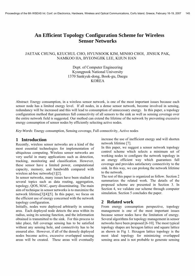
increase the use of inefficient energy and will shorten network lifetime [7]. In this paper, we suggest a sensor network topology control scheme which selects a minimum set of working nodes to configure the network topology in an energy efficient way which guarantees full coverage and provides satisfactory connectivity to the sink. In this way, we can prolong the network lifetime to the network. The rest of this paper is organized as follow. Section 2 summarizes the related work. The details of the proposed scheme are presented in Section 3. In Section 4, we validate our scheme through computer simulation. Section 5 concludes the paper. 2 Related work From energy consumption perspective, topology management is one of the most important issues because sensor nodes have the limitation of energy. Several algorithms for topology management in sensor networks have been proposed [6-10]. The most typical topology shapes are hexagon lattice and square lattice as shown in Fig 1. Hexagon lattice topology is the most ideal topology for minimizing overlapped sensing area and is not probable to generate sensing

Proceedings of the 6th WSEAS Int. Conf. on Electronics, Hardware, Wireless and Optical Communications, Corfu Island, Greece, February 16-19, 2007 145

hole. However, this type of topology does not guarantee full connectivity since it considers only the sensing coverage.

(a) The square lattice (b) The hexagon lattice

Fig. 1. The most typical topology

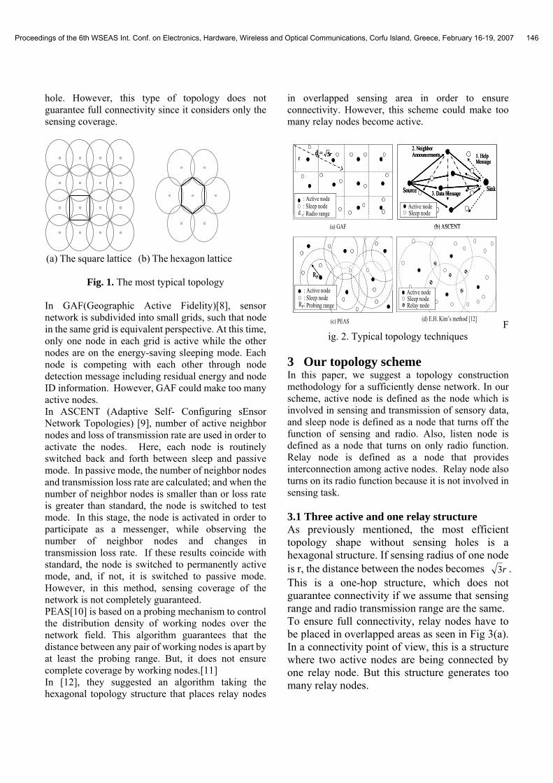
In GAF(Geographic Active Fidelity)[8], sensor network is subdivided into small grids, such that node in the same grid is equivalent perspective. At this time, only one node in each grid is active while the other nodes are on the energy-saving sleeping mode. Each node is competing with each other through node detection message including residual energy and node ID information. However, GAF could make too many active nodes. In ASCENT (Adaptive Self- Configuring sEnsor Network Topologies) [9], number of active neighbor nodes and loss of transmission rate are used in order to activate the nodes. Here, each node is routinely switched back and forth between sleep and passive mode. In passive mode, the number of neighbor nodes and transmission loss rate are calculated; and when the number of neighbor nodes is smaller than or loss rate is greater than standard, the node is switched to test mode. In this stage, the node is activated in order to participate as a messenger, while observing the number of neighbor nodes and changes in transmission loss rate. If these results coincide with standard, the node is switched to permanently active mode, and, if not, it is switched to passive mode. However, in this method, sensing coverage of the network is not completely guaranteed. PEAS[10] is based on a probing mechanism to control the distribution density of working nodes over the network field. This algorithm guarantees that the distance between any pair of working nodes is apart by at least the probing range. But, it does not ensure complete coverage by working nodes.[11] In [12], they suggested an algorithm taking the hexagonal topology structure that places relay nodes

in overlapped sensing area in order to ensure connectivity. However, this scheme could make too many relay nodes become active.

RP

: Active node: Sleep node

Probing rangeRP:

Active nodeSleep nodeRelay node

SinkSource

1. Help Message

2. NeighborAnnouncements

3. Data Message

Active nodeSleep node

(a) GAF (b) ASCENT

(c) PEAS (d) E.H. Kim’s method [12]

r


Radio ranged c:

dc= r5

RP


Probing rangeRP:




SinkSource

1. Help Message


3. Data Message

Active nodeSleep node

SinkSource

1. Help Message


3. Data Message

Active nodeSleep nodeActive nodeSleep node

(a) GAF (b) ASCENT

(c) PEAS (d) E.H. Kim’s method [12]

r


Radio ranged c:


Radio ranged c:

dc= r5dc= r5

Fig. 2. Typical topology techniques

3 Our topology scheme In this paper, we suggest a topology construction methodology for a sufficiently dense network. In our scheme, active node is defined as the node which is involved in sensing and transmission of sensory data, and sleep node is defined as a node that turns off the function of sensing and radio. Also, listen node is defined as a node that turns on only radio function. Relay node is defined as a node that provides interconnection among active nodes. Relay node also turns on its radio function because it is not involved in sensing task. 3.1 Three active and one relay structure As previously mentioned, the most efficient topology shape without sensing holes is a hexagonal structure. If sensing radius of one node is r, the distance between the nodes becomes r3 . This is a one-hop structure, which does not guarantee connectivity if we assume that sensing range and radio transmission range are the same. To ensure full connectivity, relay nodes have to be placed in overlapped areas as seen in Fig 3(a). In a connectivity point of view, this is a structure where two active nodes are being connected by one relay node. But this structure generates too many relay nodes.


In order to reduce the number of relay nodes, a structure where three active nodes are connected by one relay node should be considered, as seen in Fig 3(b). In other words, coverage is ensured by three neighbor nodes, and the relay node guarantees connectivity by activating the radio. This kind of structure must maintain an exact distance of r3 among each active node, and distance of r between active node and relay node. Nevertheless, in the sensing field where nodes are randomly stationed, it is impossible to construct such topology.

r3 r3r3 r3

(a) 2 active and 1 relay (b) 3 active and 1 relay

Fig. 3. Hexagonal lattice topology 3.2 Our topology configuration scheme Using trigonometrical function equation, Table 1 shows the most stable distance and angle formed among neighbor nodes in order to guarantee full coverage and connectivity. Here, it is assumed that neighbor nodes are located at the edge of center node’s sensing range. As seen in the Table 1, when there are three neighbor nodes, it is the most stable when distance of r3 and angle formation of 120° among the nodes are maintained. With four neighbor nodes, it is the most stable when distance of r2 and angle of 90° are maintained. As the number of node increases, the range of neighboring distance and degree that guarantees full coverage and connectivity increases, but generate many active nodes as shown in Table 1. Table 1. Relationship among nodes versus the number of neighbor nodes

The number of neighbor

nodes

Relationship Angle among active nodes

Distance among active nodes

3 120° r3

4 90° r2

5 72° r535

6 60° r

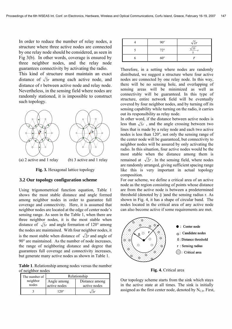
Therefore, in a setting where nodes are randomly distributed, we suggest a structure where four active nodes are connected by one relay node. In this way, there will be no sensing hole, and overlapping of sensing areas will be minimized as well as connectivity will be guaranteed. In this type of structure, entire network field will be eventually covered by four neighbor nodes, and by turning off its sensing capability while turning on the radio, it carries out its responsibility as relay node. In other word, if the distance between active nodes is less than r3 , and the angle crossing between two lines that is made by a relay node and each two active nodes is less than 120°, not only the sensing range of the center node will be guaranteed, but connectivity to neighbor nodes will be assured by only activating the radio. In this situation, four active nodes would be the most stable when the distance among them is remained at r2 . In the sensing field, where nodes are randomly arranged, giving sufficient spacing range like this is very important in actual topology composition. For our scheme, we define a critical area of an active node as the region consisting of points whose distance are from the active node is between a predetermined threshold (denoted by δ )and the sensing radius r. As shown in Fig. 4, it has a shape of circular band. The nodes located in the critical area of any active node can also become active if some requirements are met.

rδ

: Center node

: Candidate nodes

δ : Distance threshold

r : Sensing radius

: Critical area

rδ

: Center node

: Candidate nodes

δ : Distance threshold

r : Sensing radius

: Critical area

Fig. 4. Critical area

Our topology scheme starts from the sink which stays in the active state at all times. The sink is initially assigned as the first center node, denoted by NC,0. First,


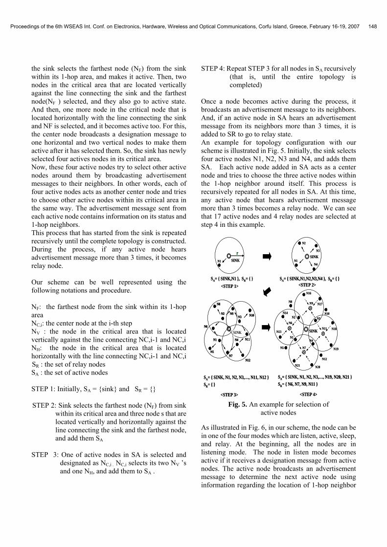
the sink selects the farthest node (NF) from the sink within its 1-hop area, and makes it active. Then, two nodes in the critical area that are located vertically against the line connecting the sink and the farthest node(NF ) selected, and they also go to active state. And then, one more node in the critical node that is located horizontally with the line connecting the sink and NF is selected, and it becomes active too. For this, the center node broadcasts a designation message to one horizontal and two vertical nodes to make them active after it has selected them. So, the sink has newly selected four actives nodes in its critical area. Now, these four active nodes try to select other active nodes around them by broadcasting advertisement messages to their neighbors. In other words, each of four active nodes acts as another center node and tries to choose other active nodes within its critical area in the same way. The advertisement message sent from each active node contains information on its status and 1-hop neighbors. This process that has started from the sink is repeated recursively until the complete topology is constructed. During the process, if any active node hears advertisement message more than 3 times, it becomes relay node. Our scheme can be well represented using the following notations and procedure. NF: the farthest node from the sink within its 1-hop area NC,i: the center node at the i-th step NV : the node in the critical area that is located vertically against the line connecting NC,i-1 and NC,i NH: the node in the critical area that is located horizontally with the line connecting NC,i-1 and NC,i SR : the set of relay nodes SA : the set of active nodes STEP 1: Initially, SA = {sink} and SR = {} STEP 2: Sink selects the farthest node (NF) from sink

within its critical area and three node s that are located vertically and horizontally against the line connecting the sink and the farthest node, and add them SA

STEP 3: One of active nodes in SA is selected and

designated as NC,i . NC,i selects its two NV ’s and one NH, and add them to SA .

STEP 4: Repeat STEP 3 for all nodes in SA recursively (that is, until the entire topology is completed)

Once a node becomes active during the process, it broadcasts an advertisement message to its neighbors. And, if an active node in SA hears an advertisement message from its neighbors more than 3 times, it is added to SR to go to relay state. An example for topology configuration with our scheme is illustrated in Fig. 5. Initially, the sink selects four active nodes N1, N2, N3 and N4, and adds them SA. Each active node added in SA acts as a center node and tries to choose the three active nodes within the 1-hop neighbor around itself. This process is recursively repeated for all nodes in SA. At this time, any active node that hears advertisement message more than 3 times becomes a relay node. We can see that 17 active nodes and 4 relay nodes are selected at step 4 in this example.

<STEP 4>

SINK

r

<STEP 1> <STEP 2>

<STEP 3>

SA= { SINK,N1 }, SR= { }

SINK

SA= { SINK,N1,N2,N3,N4 }, SR= { }

SA= { SINK, N1, N2, N3,…, N11, N12 }SR= { }

N1

N2

N3

N4N1

SINK

N1

N2N3

N4

N5

N6

N7

N8

N9 N10

N11

N12

SINKN1

N2 N3

N4

N5

N6

N7

N8 N9

N10

N11

N12

N13

N14

N16

N17

N18

N19

N20N21

SA= { SINK, N1, N2, N3,…, N19, N20, N21 } SR= { N6, N7, N9, N11 }

<STEP 4>

SINK

r

<STEP 1> <STEP 2>

<STEP 3>

SA= { SINK,N1 }, SR= { }

SINK

SA= { SINK,N1,N2,N3,N4 }, SR= { }

SA= { SINK, N1, N2, N3,…, N11, N12 }SR= { }

N1

N2

N3

N4N1

SINK

N1

N2N3

N4

N5

N6

N7

N8

N9 N10

N11

N12

N1

N2N3

N4

N5

N6

N7

N8

N9 N10

N11

N12

SINKN1

N2 N3

N4

N5

N6

N7

N8 N9

N10

N11

N12

N13

N14

N16

N17

N18

N19

N20N21

SA= { SINK, N1, N2, N3,…, N19, N20, N21 } SR= { N6, N7, N9, N11 }

Fig. 5. An example for selection of

active nodes

As illustrated in Fig. 6, in our scheme, the node can be in one of the four modes which are listen, active, sleep, and relay. At the beginning, all the nodes are in listening mode. The node in listen mode becomes active if it receives a designation message from active nodes. The active node broadcasts an advertisement message to determine the next active node using information regarding the location of 1-hop neighbor


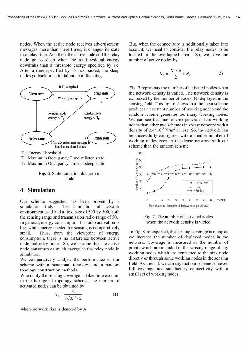
nodes. When the active node receives advertisement messages more than three times, it changes its state into relay state. And then, the active node and the relay node go to sleep when the total residual energy downfalls than a threshold energy specified by Te. After a time specified by Ts has passed, the sleep nodes go back to its initial mode of listening.

Active state

Sleep state

Relay state

Listen stateWhen TS is expired

If an advertisement message is heard more than 3 times

Residual node energy < TE


If TL is expired

Active state

Sleep state

Relay state

Listen stateWhen TS is expired

If an advertisement message is heard more than 3 times



If TL is expired

TE: Energy Threshold TL: Maximum Occupancy Time at listen state TS: Maximum Occupancy Time at sleep state

Fig. 6. State transition diagram of

node

4 Simulation Our scheme suggested has been proven by a simulation study. The simulation of network environment used had a field size of 500 by 500, both the sensing range and transmission radio range of 50. In general, energy consumption for radio activation is big, while energy needed for sensing is comparatively small. Thus, from the viewpoint of energy consumption, there is no difference between active node and relay node. So, we assume that the active node consumes as much energy as the relay node in simulation. We comparatively analyze the performance of our scheme with a hexagonal topology and a random topology construction methods. When only the sensing coverage is taken into account in the hexagonal topology scheme, the number of activated nodes can be obtained by

2/33 21 rAN = (1)

where network size is denoted by A.

But, when the connectivity is additionally taken into account, we need to consider the relay nodes to be located in the overlapped area. So, we have the number of active nodes by

11

2 26 NNN +

×= (2)

Fig. 7 represents the number of activated nodes when the network density is varied. The network density is expressed by the number of nodes (N) deployed in the sensing field. This figure shows that the hexa scheme produces a constant number of working nodes and the random scheme generates too many working nodes. We can see that our scheme generates less working nodes than other two schemes in sparse network with a density of 2.4*10-5 N/m2 or less. So, the network can be successfully configured with a smaller number of working nodes even in the dense network with our scheme than the random scheme.

0

50

100

150

200

250

300

8 12 16 20 24 28 32 36 40 44Network density (the number of deployed nodes per unit area )

Num

ber o

f wor

king

nod

es

Our schemeHexaRandom

(10-4N/m2 )0

50

100

150

200

250

300

8 12 16 20 24 28 32 36 40 44Network density (the number of deployed nodes per unit area )

Num

ber o

f wor

king

nod

es

Our schemeHexaRandom

(10-4N/m2 )

Fig. 7. The number of activated nodes when the network density is varied

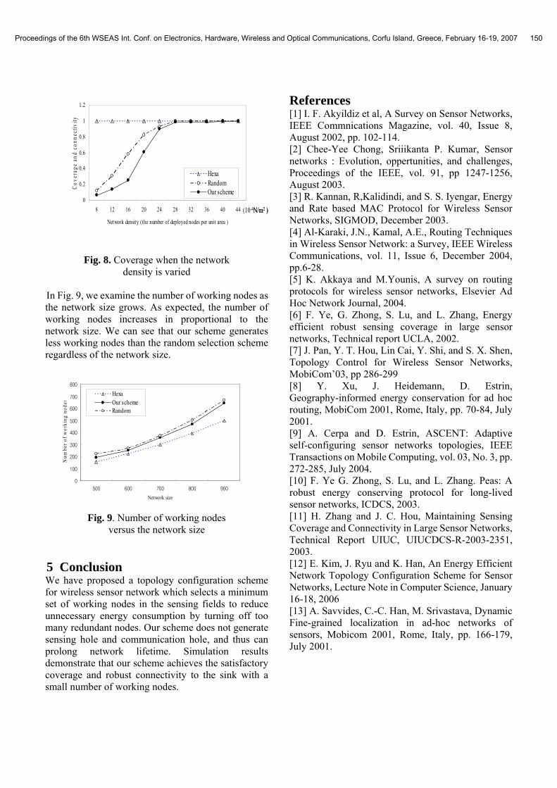
In Fig. 8, as expected, the sensing coverage is rising as we increase the number of deployed nodes in the network. Coverage is measured as the number of points which are included in the sensing range of any working nodes which are connected to the sink node directly or through some working nodes in the sensing field. As a result, we can say that our scheme achieves full coverage and satisfactory connectivity with a small set of working nodes.


0

0.2

0.4

0.6

0.8

1

1.2

8 12 16 20 24 28 32 36 40 44

Network density (the number of deployed nodes per unit area )

Cove

rage

and

con

nect

ivity

HexaRandomOur scheme

(10-4N/m2 )0

0.2

0.4

0.6

0.8

1

1.2

8 12 16 20 24 28 32 36 40 44

Network density (the number of deployed nodes per unit area )

Cove

rage

and

con

nect

ivity

HexaRandomOur scheme

(10-4N/m2 )

Fig. 8. Coverage when the network

density is varied In Fig. 9, we examine the number of working nodes as the network size grows. As expected, the number of working nodes increases in proportional to the network size. We can see that our scheme generates less working nodes than the random selection scheme regardless of the network size.

0

100

200

300

400

500

600

700

800

500 600 700 800 900

Network size

Num

ber o

f wor

king

nod

es

HexaOur schemeRandom

Fig. 9. Number of working nodes

versus the network size

5 Conclusion We have proposed a topology configuration scheme for wireless sensor network which selects a minimum set of working nodes in the sensing fields to reduce unnecessary energy consumption by turning off too many redundant nodes. Our scheme does not generate sensing hole and communication hole, and thus can prolong network lifetime. Simulation results demonstrate that our scheme achieves the satisfactory coverage and robust connectivity to the sink with a small number of working nodes.

References [1] I. F. Akyildiz et al, A Survey on Sensor Networks, IEEE Commnications Magazine, vol. 40, Issue 8, August 2002, pp. 102-114. [2] Chee-Yee Chong, Sriiikanta P. Kumar, Sensor networks : Evolution, oppertunities, and challenges, Proceedings of the IEEE, vol. 91, pp 1247-1256, August 2003. [3] R. Kannan, R,Kalidindi, and S. S. Iyengar, Energy and Rate based MAC Protocol for Wireless Sensor Networks, SIGMOD, December 2003. [4] Al-Karaki, J.N., Kamal, A.E., Routing Techniques in Wireless Sensor Network: a Survey, IEEE Wireless Communications, vol. 11, Issue 6, December 2004, pp.6-28. [5] K. Akkaya and M.Younis, A survey on routing protocols for wireless sensor networks, Elsevier Ad Hoc Network Journal, 2004. [6] F. Ye, G. Zhong, S. Lu, and L. Zhang, Energy efficient robust sensing coverage in large sensor networks, Technical report UCLA, 2002. [7] J. Pan, Y. T. Hou, Lin Cai, Y. Shi, and S. X. Shen, Topology Control for Wireless Sensor Networks, MobiCom’03, pp 286-299 [8] Y. Xu, J. Heidemann, D. Estrin, Geography-informed energy conservation for ad hoc routing, MobiCom 2001, Rome, Italy, pp. 70-84, July 2001. [9] A. Cerpa and D. Estrin, ASCENT: Adaptive self-configuring sensor networks topologies, IEEE Transactions on Mobile Computing, vol. 03, No. 3, pp. 272-285, July 2004. [10] F. Ye G. Zhong, S. Lu, and L. Zhang. Peas: A robust energy conserving protocol for long-lived sensor networks, ICDCS, 2003. [11] H. Zhang and J. C. Hou, Maintaining Sensing Coverage and Connectivity in Large Sensor Networks, Technical Report UIUC, UIUCDCS-R-2003-2351, 2003. [12] E. Kim, J. Ryu and K. Han, An Energy Efficient Network Topology Configuration Scheme for Sensor Networks, Lecture Note in Computer Science, January 16-18, 2006 [13] A. Savvides, C.-C. Han, M. Srivastava, Dynamic Fine-grained localization in ad-hoc networks of sensors, Mobicom 2001, Rome, Italy, pp. 166-179, July 2001.


An Efficient Topology Configuration Scheme for Wireless Sensor Networks

Documents