An Efficient Swarm Neighborhood Management for a 3D Tactical Simulator

An Efficient Swarm Neighborhood Management for a 3D Tactical Simulator

Russel Ahmed Apu, Marina L. Gavrilova

Department of Computer Science, University of Calgary

2500 University Drive NW, Calgary, AB, Canada T2N 1N4

{[email protected], [email protected]}

Abstract

The paper presents a unique utilization of the

Dynamic Delaunay Triangulation (DT) to devise a

highly efficient algorithm for the neighborhood

adjacency management which is a crucial component

of a swarm-based simulation. This algorithm allows

fast computation of the swarm neighborhood which is

required to implement Boids flocking rules. The

method also provides an efficient mechanism to detect

and manage object collisions. This unique utilization of

DT based data structures was applied to a new 3D

tactical swarm simulation called the Battle Swarm. The

result was a very high speed of simulation, which made

complex application of genetic evolution possible for

goal-based swarms in a three dimensional space. The

method's effective and complex emergent behavior was

successfully demonstrated by the Battle Swarm

Simulator. In addition, the experimental section

confirms that the method was highly efficient and can

be used in similar applications.

Keywords

Dynamic Delaunay Triangulation, Voronoi

Diagram, Battle Swarm, Swarm Intelligence, Genetic

Algorithm, Physically Based Modeling, DCEL.

1. Introduction:

Swarm Intelligence (SI) is the property of a system

whereby the collective behaviors of (unsophisticated)

agents interacting locally with their environment cause

coherent functional global patterns to emerge. SI

provides a basis with which it is possible to explore

collective (or distributed) problem solving without

centralized control or the provision of a global model

[4]. Agents in an SI based system have limited

perception or intelligence and cannot individually carry

out the task that is designated to the swarm.

Nevertheless, by regulating the behavior of the agents

in the swarm, one can demonstrate emergent behavior

and intelligence as a collective phenomenon [14][18].

The Battle Swarm model is based on an interesting

gaming scenario. It is a carefully chosen problem to

reflect a more general goal-based 3D tactical swarm

simulation [5]. In this simulation, there are two

competing entities. Firstly, a Battle-ship with a

complex 3D structure is deployed in free space. This

structure is represented as set of polygons using DCEL

[2]. Secondly, a swarm of missiles (point objects) are

launched from a distance to attack and destroy the

battle-ship. The battle-ship has multiple point defense

energy cannons that are capable of firing at arbitrary

direction at a specific rate of fire (predefined to 600

rounds per minute). The angular coverage of each

turret is limited to a threshold (predefined to 30

degrees). A particular point defense cannon is only

able to acquire and attack targets that are within its

coverage zone (Fig. 1). Choice of the target is acquired

based on a Threat of Approach function. Once the

target is chosen, a firing solution for each turret is

obtained numerically by extrapolating the missiles

current trajectory.

Figure 1:Figure 1:Figure 1:Figure 1: Space battle tactics simulation: missiles versus point defense

This kind of simulation requires a significant

amount of computation to even process one frame of

the simulation [14][18]. To apply genetic algorithm for

complex emergent behavior the simulation must be

executed for hundreds of generations resulting in

millions of simulation steps [11]. As a result, the

efficiency of the simulation becomes a major factor in

deciding whether or not a 3D simulation of such

magnitude of complexity is even feasible. In general,

majority of the computational tasks in such a

simulation can be divided into the following processes:

• Computation of neighborhood based on circle

of influence

• Collision detection and response

• Computation of cone of influence for each

point defense

This paper presents a unique utilization of the

Randomized Incremental Delaunay Triangulation

method to devise a highly efficient technique to aid the

three aforementioned processes [13]. The method is

found to be effective and reliable. It is simple to

implement and can be applied to a variety of similar

3D spatial temporal simulations [4].

2. Literature Survey

Behavioral studies among social biological entities

such as insects were of interest for scientists for a long

time [3][4][15]. Flight formation of a flock of birds

[16], stratification and construction of an ant/termite

colony [3][15] or a school of fish swimming in

formation [7][16] are all surprisingly complex tasks

given the intelligence of each individual agent.

Recently, biologists and computer scientists in the field

of artificial life have modeled biological swarms to

understand how social animals interact, achieve goals,

and evolve [4][14][15]. Engineers also become

increasingly interested in swarm behavior since the

resulting swarm intelligence can be applied in

optimization (e.g. in telecommunicate systems)

[5][11], robotics [5][7][18], traffic patterns in

transportation systems [17] and military applications

[5][7]. The idea of using SI for battle tactics and war

games is relatively new and active area of research [7].

However, because of the complexity of these systems,

it cannot be modeled efficiently using a conventional

swarm simulation engine.

In our study, we discovered that a majority of the

commercial swarm simulations employ inefficient

algorithms to determine the neighborhood of agents

and implements simple collision techniques by limiting

to point, spherical and planar objects. The use of such

methods is feasible only if a certain flocking logic is

being tested or a small scale evolutionary system is

being developed [16]. Therefore, for more complex

simulations such as the one outlined in this paper, a

sophisticated and efficient algorithm is required to

handle the task of neighborhood management and

collision detection in three dimensions.

We identified several popular approaches for

collision detection and neighborhood management in

the literature. First technique is a simple grid based

approach [2]. Although this method is fairly effective,

it is found to be inefficient in dynamic environment

where congestion or dispersion may arise periodically.

Another popular approach is to use K-D Tree based

methods for efficient query of proximal information

[1][2][9]. These methods relatively more efficient for

query, however, they require significant build time for

the data structure that may render the whole simulation

inefficient. Last but not the least, an efficient

triangulation method can be employed, where a full

construction of the data structured is carried out at the

beginning of the simulation and at each step the

structure is revised by taking advantage of the spatial-

temporal coherence [8][13]. The Delaunay

Triangulation [6] method is the prime candidate in this

category for several reasons. Firstly, it is a robust data

structure for proximity management [9]. Secondly, it is

a dual of a Voronoi Diagram and therefore rich in

many useful geometric properties [9][10]. Finally, a

broad domain of literature is dedicated to the analysis

and improvement of this method rendering it a highly

efficient and well studied data structure in

computational geometry [6][8][9][12][13].

After careful consideration, we propose to use

Delaunay Triangulation for the aforementioned

problem and employ a clever scheme for collision and

neighborhood management. The paper is organized as

followed. Section three provides a detailed description

of the problem followed by the description of the data

structures and techniques employed. Section four

provides the analysis and experimental results. This is

followed by the summary and conclusion in Section 5.

3. Method Description

In this section, we outline the problem as a special

class of swarm simulation in three dimensions that

employs complex emergent strategies and outline its

solution. The simulation framework is generic and can

be applied to most three dimensional swarm

simulations. Later, we provide a novel approach to

compute swarm adjacency and neighborhood

management for the problem described below.

3.1. The Game of the Battle Swarms

For the simulation of emergent complex strategy,

we devised a game carefully chosen to reflect the

complexity of a goal-based 3D tactical swarm system

[5][7]. The game is based on attack, evasion and

defense. While the missile sets strategy to strike the

target, the battle ship prepares to shoot down as many

missiles as possible. Each attempt to destroy the target

is called an Attack-Run. The effectiveness of an

Attack-Run equals to the number of missiles hitting the

target. Therefore, the outcome of the game is easily

quantifiable.

On the other hand, the interaction between missiles

and the battleship is complex and nontrivial. As a

result, war strategies may emerge in which a local

penalty (i.e. sacrificing a missile) can optimize global

efficiency (i.e. deception strategy).

The following sub section clearly identifies the

objects and the context of the game:

• The Missile: The limited capability of a missile

makes it an excellent candidate for a swarm-based

agent. Each missile has a pool of basic actions (Fig.

2) it can carry out (i.e. roll and pitch). Each missile is

autonomous and decides its course of action based

on the location of the target, incoming fire and other

missiles within the limited sensory range. Each

missile has to choose between following other

missiles or the target. This behavior of following

peers is known as the Boids Flocking (Fig. 3) [16].

• The Battle Ship Defense: The Battle-ship defense

includes several point defense turrets. Each turret

evaluates all visible targets within the range using a

threat function and selects the missile that poses the

highest threat. This is done by computing a list of

missiles within a conic coverage zone for each turret.

The turret computes a firing solution based on the

trajectory of the missile. A divergence probability is

estimated by analyzing the last few actions of the

missile and the region of uncertainty (Fig. 1).

3.2. The Computational Complexity

The computational complexity of the system arises

from the fact that agents (such as missiles and turrets)

interact with each other based on local information

such as proximity, coverage, visibility etc. [3][4].

These computational challenges exist not only in the

problem stated above but most swarm-based

simulations in general. Furthermore, the complexity is

increased significantly in three dimensions [7][19] over

some of the two dimensional simulations (i.e.

simulation of human crowd on a plane [14]).

To understand the requirement for the data-structure

optimization, it important to design a robust and

predictive dynamic system. Therefore, we propose the

following system of equation for the missile dynamics:

( )

21

2

tt t

damp

t t t t

k x x tx

x x x t x t

+∆

+∆

+ ∆ = + ∆ + ∆

� ���

� ��

(1)

Here , t t t tx x+∆ +∆

� are the new position and velocity

of a node respectively and , , t t tx x x� �� are the last

positions, velocity and acceleration. t∆ is the time-

step interval and dampk is the kinetic dampening

constant. This system of forward differential equations

is predictive in a sense that regardless of the discrete

Figure 2: Figure 2: Figure 2: Figure 2: The control mechanism for missile navigation

Figure Figure Figure Figure 3333:::: Boids flocking rule: Peers in the inner sphere are deflected while the node is attracted

towards peers inside the outer sphere.

time-stepping interval, the system can be made to

converge to a terminal velocity for each dynamic

object. This terminal velocity maxx� can be specified by

computing corresponding dampening constant dampk as

followed:

max

1damp

x tk

x

∆= −��

� (2)

The dynamic system described above provides a

predictive motion pattern. In a predictive system, a

position can be estimated from a particular trajectory

pattern (i.e. a circular trajectory). In ordinary forward

Euler dynamic system, the trajectory prediction is not

possible because the accumulative error vary widely

based on particle speed and status of acceleration. By

using a terminal velocity and carefully chosen

dampening equation, we minimize the variation of

accumulative errors during the time stepping. This

important property is required to obtain a firing

solution.

Because of the terminal velocity, and the temporal

cohesion observed in Boids Flocking [16], the dynamic

objects in the scene satisfy a frame-to-frame coherence

property. An optimized data structure needs to take

advantage of this property, imposing minimal

computational load over a given interval.

The task of the computational engine of a 3D

swarm simulation is several-fold. Firstly, it must

present the Agent’s AI callback, with a list of

neighbors within a given spherical region of influence

(Fig. 3). This requires the preparation of a

neighborhood table in which, Row i contains the list

of peers that are within the outer spherical region of

radius outerR (Fig. 3). A similar table is also required

for the conic coverage of turrets. Finally, a table of

collision needs to be constructed, where each row

stores a list of swarm agents that are in contact with the

stationery object. To provide these solutions, we

propose to use the Dynamic Delaunay Triangulation

data structure which is more robust and efficient than

other static data structures such as the regular grids and

TIN [2][8][9]. The following subsections discussed the

general incremental DT algorithm and our unique

scheme to solve the aforementioned computational

problems.

3.3. The General Delaunay Triangulation

The Delaunay Triangulation is a useful data

structure in computational geometry because it is a

dual of a Voronoi Diagram [2][6][10]. Since the DT

has an edge for every pair of adjacent VD regions, it is

connected to its nearest neighboring sites [2]. This

construct allows a robust adjacency/proximity

representation that can be used in many geometric

problems. In our case, the connectivity of DT can be

directly used to compute the neighborhood of the

swarm agents. In addition, the border edges of the DT

forms the Convex Hull of the point set [2]. Therefore,

it can be used to compute the collision table efficiently.

The conic influence table can be constructed by

approximating a cone by four bounding half planes and

performing an inclusion test.

It has been shown that a 2D DT can be constructed

by a randomized algorithm in ( log )O n n time [6] and

with certain optimizations it could be constructed in

linear expected time in the average case [13]. The 3D

DeWall incremental algorithm is relatively more

complicated [12]. It can be constructed in 3( )O n

worst case time although the expected time reported

can be lower (i.e. Quadratic runtime) [13].

(a)(a)(a)(a) (b)(b)(b)(b) (c)(c)(c)(c)

Figure 4:Figure 4:Figure 4:Figure 4: Incremental Construction of the Delaunay Triangulation. (a)(a)(a)(a) Insertion of a new site

(b)(b)(b)(b) Perform the in-circle test (c)(c)(c)(c) Flip and perform in-circle test recursively

The most popular incremental approach to DT

construction is outlined below. First, a bounding

triangle is built such that it includes all sites. At each

step, a random site is chosen and inserted in the DT

structure. For that purpose, the bounding simplex

(triangle or tetrahedron) of the site is identified and

subdivided to include the new site. After that, each

opposite edge is tested for its in-circle property (or in-

sphere property in 3D) and the edge/face is flipped if

this property is violated. If a flip operation is actuated,

then a recursive in-circle test is executed for the new

opposing sides. The insertion is complete when all the

neighboring edges pass the test.

3.4. The Dynamic Layered Delaunay

Triangulation (LDT)

We discovered that the actual implementation of the

3D DT is not only a difficult task, but also the runtime

is far too inefficient for practical use when applied to a

large number of dynamic swarm particles. Therefore,

we propose the following novel solution.

We propose that the entire spatial bound be divided

into K regions and for each region a planar DT is

computed by projecting the points along the principle

axis (Fig. 5). The neighborhood of a site is then the

union of its entire neighborhood in the K set of DT.

The first step in this algorithm is to find the Axis

Aligned Bounding Box (AABB) of the swarm sites

(fig. 5a) [2]. In each simulation two Principle axes (two

of the X, Y and Z axis) are chosen. They are called the

splatting axis. Although for this algorithm, any choice

of splatting axes may suffice, carefully choosing a

subset may enhance performance. A rule of thumb we

determined was to choose the two splatting axes that

have the minimal spatial dispersion during the overall

simulation. In other word, we exclude the axis that is

along the longest edge of all AABBs. The reason for

doing this is to minimize the thickness of each slab.

For example, because of the way the missile swarms in

our application are generated (Large X-Axis offset)

with respect to the location of the target (origin), the Y

and Z axis were chosen as the splatting axes.

(a)(a)(a)(a) Three initial quadrants (b)(b)(b)(b) Left quadrant expanding (c)(c)(c)(c) execution of Case 5 & right quadrant shrinking

Figure Figure Figure Figure 6666:::: Execution of the Merge/split process in Method 1, Case 5.

(a)(a)(a)(a) Global AABB (b)(b)(b)(b) Subdivision along (c)(c)(c)(c) Projection along splatting axis one of the splatting axis and construction of an LDT

Figure 5:Figure 5:Figure 5:Figure 5: Construction of the Layered Delaunay Triangulation.

The next step is to divide the global swarm AABB

into K quadrants (Fig 5b). Each quadrant assumes the

boundary of the global AABB except the splatting

axis. At each step, the quadrant containing the maximal

splatting axis dispersion is selected and divided. For

robustness additional conditions may be imposed. One

important condition is that at least 2 divisions must

exist for each splatting axis. This guarantees that every

point is included in atleast two mutually orthogonal

quadrants.

For each of these K regions, the points are projected

along the splatting axis on a plane and a DT is

computed and stored (Fig. 5c). For the dynamic

maintenance of the data structure the following

algorithm must be invoked at each computational time-

step:

Method 1: Adjust Layered DT

For each swarm node in the system consider the

following cases:

1. Internal Transition: The swarm node remains in

the same quadrant, however, the length of one of

its edges changes by a threshold τ (i.e. 85%τ =

in Battle Swarm). This node is marked as invalid,

and the recursive in-circle test is applied at a later

step.

2. Inter-quadrant Transition: When a node crosses

the planar boundary between two adjacent

quadrants (along the splatting axis), the node is

deleted from the old quadrant. The linked vertices

are triangulated and the circle test is performed

accordingly. The node is then added to the new

quadrant (standard DT point insertion).

3. External Transition: The swarm node exits the

boundary of the current quadrant outside the

AABB. In this case, the boundary is extended to

include the point and the region grows (Fig. 6).

4. Collapsing Transition: When a quadrant has no

swarm nodes, it is deleted. The quadrant with the

maximum splatting axis dispersion is split in two.

5. Size Optimization Transition: First, two adjacent

quadrants with the least dispersion is chosen. If

their combined dispersion is less than the quadrant

with the largest splatting axis dispersion then the

region pair is merged and the largest quadrant is

split into two quadrants (Fig 6). Each execution

loop can have at most one such transition.

All split/merge operation is carried out by

reconstructing the Delaunay Triangulation(s). One

important thing to be mentioned here is that the swarm

simulation does not require a precise Delaunay

Triangulation. Degeneracy can be allowed to a certain

extent so that the number of flips is minimized. In our

case, the edge tolerance 85%τ = was a good choice

reducing the number of flips significantly and yet

minimally affecting the neighborhood computation.

The choice of τ vary depending on the swarm density

and the motion pattern. The value of τ can be

determined by a simple trial and error method before

the execution of the Genetic Algorithm.

For optimization purpose, the actual algorithm for

case 1 in Method 1 was implemented in a separate step.

This is carried out by marking the opposite vertex pair

of all offending edge and then adjusting each marked

vertex.

3.5. Computation of the Swarm Neighborhood

and the Collision Table

The computation of the swarm neighborhood is a

straight-forward task given the layered DT

representation. A general algorithm is given below:

Method 2: Compute Neighborhood

Input: DT[], K

Output: NB[]

1. Proc. Neighbors(DT[], K, NB[]) 2. Initialize(NB)

3. for i�1 to K do

4. for each Edge e in NB[i] do

5. if Length[e]< outerR then

6. AddTable(NB,e.v1,e.v2)

This algorithm functions by assuming that each

node belongs to more than one overlapping orthogonal

LDT. Therefore, the union of the nearest neighbors

obtained from those LDT, compose the three

dimensional neighborhood of a node. For example, if a

node is near the wall of a quadrant and misses

neighbors located in the adjacent quandrant then the

orthogonal quadrant containing that node will also

contain the nodes that were missed by the first

quadrant.

The test for collision is also very simple. At a

preprocessing step, the convex hull of the static object

is computed by projecting the 3D polygonal model

along the splatting axis. The collision test is performed

by quick elimination of points belonging to a quadrant

that does not include the stationery object. For

intercepting quadrants, each point is filtered through a

bounding box test followed by a quick convex hull

intersection test. If a point passes this intersection test

for each quadrant it belongs to, a line-polygon

intersection test is performed between the 3D

representation of the object and the line between the

last two consecutive positions of the node. This

method is both precise and highly efficient.

Finally, the conic coverage is computed by

approximating to four half planes for each cone and

finding the intersection with a bounding region when it

is created (or modified). Points are tested quickly for

inclusion by a series of orientation tests. If an accurate

conic coverage is required, an additional angular test

can be performed on the points that passed the previous

point-plane orientation tests. Points that are in the

frustum but not inside the cone can be eliminated this

way.

4. Analysis of the result:

It should be noted first that in a swarm simulation,

the neighborhood table need not be precise. For

example, it does not matter if the number of neighbors

identified for a node is 6 when there should be 8 (2

neighbors are missed). If such is the case, the Boids

flocking is minimally affected. We executed a

simulation with known characteristics and discovered

that even with a 20% degeneracy, there is no

noticeable difference in the result or the flocking

behavior of the swarm. In our implementation, the

degeneracy rate is approximately 4.6% with 85%τ =

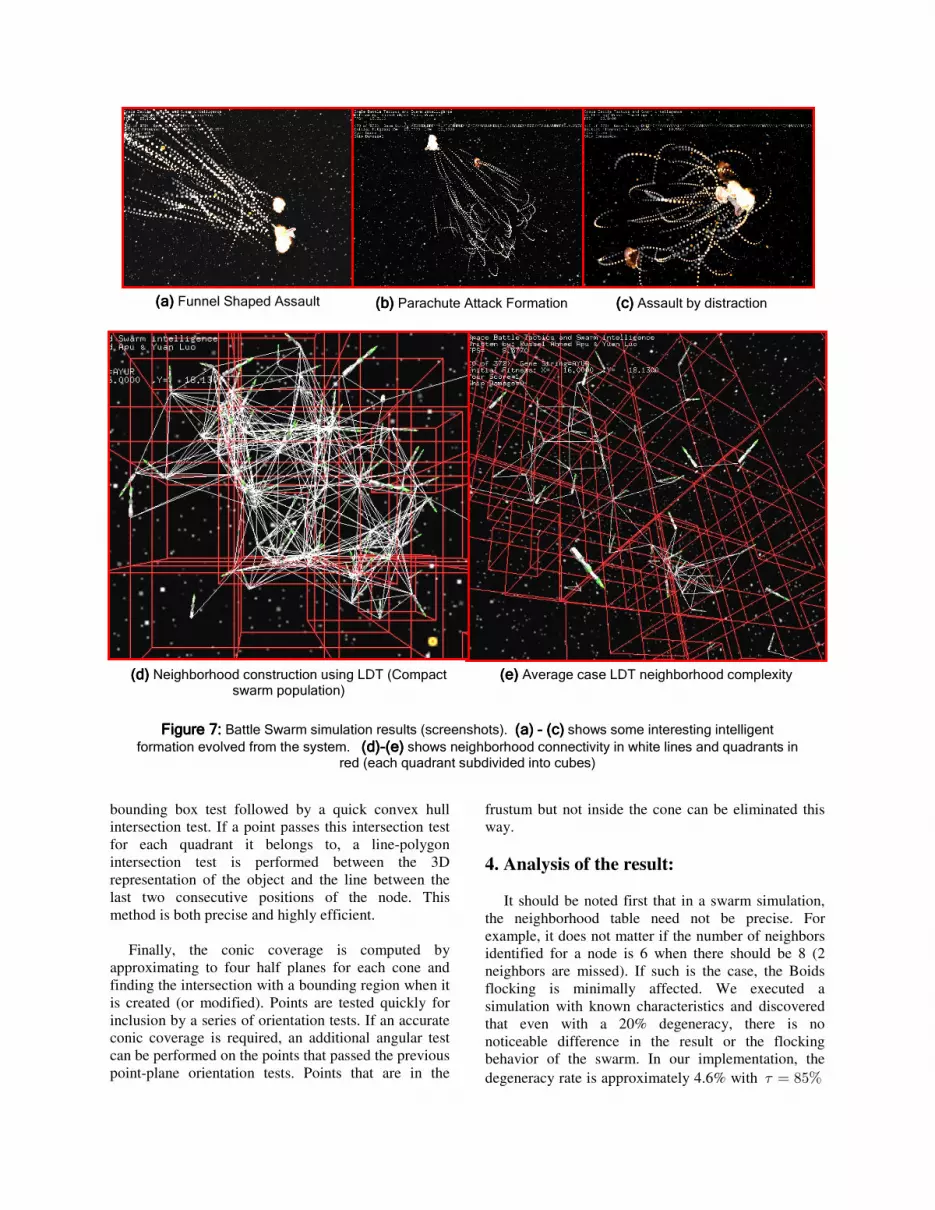
(a)(a)(a)(a) Funnel Shaped Assault ((((bbbb)))) Parachute Attack Formation

Figure 7:Figure 7:Figure 7:Figure 7: Battle Swarm simulation results (screenshots). (a) (a) (a) (a) –––– (c) (c) (c) (c) shows some interesting intelligent

formation evolved from the system. (d)(d)(d)(d)----(e)(e)(e)(e) shows neighborhood connectivity in white lines and quadrants in red (each quadrant subdivided into cubes)

((((cccc)))) Assault by distraction

((((dddd)))) Neighborhood construction using LDT (Compact swarm population)

((((eeee)))) Average case LDT neighborhood complexity

and K=8 (number of swarms, n=500). One important

aspect is that most swarm simulation provides an inner

radius that prevents nodes from overcrowding. This

makes the application of Layered DT highly effective

for such swarm problems.

It may appear from the algorithm that the system is

performing too much computation for neighborhood

and collision management. We now show that this is

not the case. Firstly, we know that a DT is a planar

Graph. As a result, it can be shown that the system has

at most ( )O n K− edges. Since K is a constant, the

algorithm in Method 2 executes in ( )O n time. The

only large computation is the first construction of the

K Layered DT in ( log )O n n time. By careful

implementation of the algorithm, it can be carried out

in linear expected time. After that, the only

computation needed to maintain the data structure is

Method 1. Although Case 1 has a worst case runtime

of ( log )O n n , in reality the average runtime is

(1)O due to frame-to-frame coherence and degenerate

edge tolerance τ . Case 2-4 also executes in roughly

constant time (or at least less than linear time). The

only major operation is Case 5 in which a merge and

split operation is applied on the LDT Structures. The

worst case runtime is ( log )O n n . But our analysis of

the runtime measurements indicates that the actual

execution takes less than linear time. Firstly, when a

split or merge occurs, one of the merged quadrants

usually contains very few nodes. Similarly, the newly

created quadrant (called a leading front) has minimal

number of nodes. In addition, the occurrences of Case

5 is sparse (occurs when the global formation of the

swarm gets dispersed, shrunk or displaced

significantly). As a result, the overall execution of

Method 1 is highly efficient.

To perform a runtime analysis we implemented the

entire swarm system including the computational,

rendering and GA engine. The application was

executed in an AMD Sempron XP™ 1.8GHz

workstation with an ATI Radeon graphics adapter. The

performance was measured using the Windows Query

Interface API which is accurate to several

microseconds. When measurement was taken, we

switched off non critical sub-systems such as UI,

rendering and particle engine.

The runtime performance of the system was

unprecedented. With approximately 100 nodes we

were able to achieve approximately 357 FPS. At this

rate, we were able to evolve a 1000 generations in less

than 5 hours on a single workstation. The frame rate

drops to 97.2 FPS when the number is nodes is

increased to 500 (and K=12). Some interesting results

are provided in Fig. 7. These are screen shots taken

directly from the Battle Swarm application. Fig. 7(a-c)

demonstrates that using our method it is possible to

achieve sophisticated evolutionary swarm intelligence.

Fig 7(d-e) visualizes the neighborhood connectivity in

different context using our method. Thus, we conclude

that the method was highly effective and efficient.

5. Conclusion:

In this paper, we presented a novel utilization of the

Delaunay Triangulation to solve the neighborhood

computation problem of a 3D tactical swarm

simulation called the Battle Swarm. The method was

robust, easy to implement and yet highly efficient. The

experimental section indicates that the performance of

this new method was unprecedented. This new method

would help designing complex 3D swarm simulations

that can exhibit complex strategic swarm intelligence.

Finally, the idea of utilizing a layered Dynamic

Delaunay Triangulation to resolve neighborhood and

collision of the battle swarm is unique and can be also

used in other applications.

6. Acknowledgement:

This project was funded partially by the NSERC

and the GEOIDE grant.

7. References

[1] Benitez, A., Ramirez, M. C. and Vallejo, D.

Collision Detection Using Sphere-Tree

Construction, 15th International Conference on

Electronics, Communications and Computers

(CONIELECOMP'05), pp. 286-291, 2005.

[2] Berg, M. D., et al. Computational Geometry:

Algorithms and Applications, Springer-Verlag

Berlin Heidelberg, ISBN 3-540-61270-X, 1997.

[3] Bonabeau, E. Stigmergy (special issue). Artificial

Life, 5(2).

[4] Bonabeau, E., Dorigo, M. and Theraulaz, G.

Swarm Intelligence: From Natural to Artificial

Systems, NY: Oxford Univ. Press, 1999

[5] Cebrowski, A. K., et al., Network Centric

Warfare: Its Origin and Future. Proceedings of the

Naval Institute, No. 124(1), pp 28-35, 1998.

[6] Cignoni, P., Montani, C., and Scopigno, R. A Fast

Divide and Conquer Delaunay Triangulation

Algorithm in Ed. Computer-Aided Design,

Elsevier Science, vol.30(5), April 1998, pp.333-

341.

[7] Doty, K. L., et al. An Autonomous Micro-

Submarine Swarm and Miniature Submarine

Delivery System Concept. In Proceedings of the

Florida Conference on Recent Advanced in

Robotics (Melbourne, Florida). pp 131-138, 1998.

[8] Edelsbrunner, H., Preparata, F. P. and West, D. B.

Tetrahedrizing point sets in three dimensions.

J. Symbolic Comput., 10(3-4), pp 335-347, 1990.

[9] Gavrilova, M, and Rokne, J. Collision detection

optimization in a multi-particle system,

International Journal of Computational Geometry

and Applications, vol 13 No 4, August 2003.

[10] Gavrilova, M. and Rokne, J. “Updating the

Topology of the Dynamic Voronoi Diagram for

Circles in Euclidean d-dimensional Space”.

Journal of Computer Aided Geometric Design, vol

20, pp 231-242, 2003.

[11] Iba, H. Emergent cooperation for multiple agents

using genetic programming. Parallel Problem

Solving from Nature. Berlin, 1996.

[12] Joe, B. Construction of three-dimensional

Delaunay triangulations using local

transformations. Comput. Aided Geom. Design,

8(2):123-142, May 1991.

[13] Mücke, E., Saias, I., and Zhu, B. Fast Randomized

Point Location without Preprocessing in Two- and

Three-dimensional Delaunay Triangulations.

Proceedings of the 12th Annual Symposium on

Computational Geometry, pages 274-283, 1996.

[14] Raupp, S. and Thalmann, D. Hierarchical Model

for Real Time Simulation of Virtual Human

Crowds, IEEE Transactions on Visualization and

Computer Graphics 7(2) (2001) 152-164

[15] Resnick, M. Turtles, Termites, and Traffic Jams

Explorations in Massively Parallel Microworlds.

MIT Press, 1997

[16] Reynolds, C. W. Flocks, Herds, and Schools: A

Distributed Behavioral Model, in Computer

Graphics, 21(4) (SIGGRAPH '87 Conference

Proceedings), 1987, pp. 25-34.

[17] Sauter, J. A., et al. Performance of digital

pheromones for swarming vehicle control.

Proceedings of the fourth international joint

conference on Autonomous agents and multiagent

systems AAMAS, 2005, pp. 903-910.

[18] Shen, W. M., Will, P., Galstyan, A., and Chuong,

C. M. Hormone-Inspired Self-Organization and

Distributed Control of Robotic Swarms,

Autonomous Robots, Volume 17 Issue 1, 2004,

pp. 700-712.