An efficient non-enumerative method to estimate path delay fault coverage

240 IEEE TRANSACTIONS ON COMPUTER-AIDED DESIGN OF INTEGRATED CIRCUITS AND SYSTEMS, VOL. 13, NO. 2, FEBRUARY 1994

An Efficient Nonenumerative Method to Estimate the Path Delay Fault Coverage in Combinational Circuits

Irith Pomeranz, Member, IEEE, and Sudhakar M. Reddy, Fellow, IEEE

Abstruct- A method to estimate the coverage of path delay faults of a given test set, without enumerating paths, is proposed. The method is polynomial in the number of lines in the circuit, and thus allows circuits with large numbers of paths to be considered under the path delay fault model. Several levels of approximation, with increasing accuracy and increasing polynomial complexity, are proposed. Experimental results are presented to show the effectiveness and accuracy of the estimate in evaluating the path delay fault coverage. Combining this non-enumerative estimation method with a test generation method for path delay faults would yield a cost effective method to consider path delay faults in large circuits, which are beyond the capabilities of existing test generation and fault simulation procedures, that are based on enumeration of paths.

I. INTRODUCTION WO COMMON fault models were proposed for defects T that change the timing behavior of a circuit, the gate delay

fault model (that includes the transition fault model as a special case) and the path delay fault model [1]-[7]. Both models have received wide attention in terms of test generation, fault simulation and synthesis-for-testability procedures [ 11-[26]. While the number of gate delay faults in a circuit is linear in the number of lines in the circuit, the number of path delay faults is, in the worst case, exponential in the number of lines. In most practical cases, the number of paths in a circuit is very large, making it impossible to enumerate all paths for the purposes of test generation and fault simulation. To overcome this problem, some methods consider only subsets of paths, e.g., only the longest paths are considered in [7], [13]. However, even the number of longest paths can be very large, e.g., for optimized circuits, paths tend to have the same propagation delays [27]. In this work, we propose a method to estimate the number of path delay faults detected by a given test set, without enumerating the paths (neither the complete set of paths nor the detected faults are enumerated), in time which is polynomial in the size of the circuit. The problem of handling large numbers of paths (e.g., using the complete set of paths as in [4] or storing the detected faults as in [ 121) is thus alleviated. The computed estimate is pessimistic, i.e., the true fault coverage is not smaller than the estimated one. As the degree of the complexity polynomial is increased, better estimates are obtained. In the limit, if the degree of the polynomial is allowed to be of the order of number of

Manuscript received August 21, 1992. This work was supported in part by the NSF under Grant MIP-9220549. This paper was recommended by Associate Editor C. Kime.

The authors are with the Electrical and Computer Engineering Department, University of Iowa, Iowa City, IA 52242.

IEEE Log Number 9213656.

lines in the circuit instead of being a constant, thus resulting in exponential complexity, the exact number of path delay faults detected is obtained. We show experimentally that a very good estimate of the number of path delay faults detected is obtained even for the first-order approximation, in which the degree of the complexity polynomial is two. It thus becomes practically possible to consider large numbers of path delay faults during fault simulation, without enumerating the faults. This also allows consideration of a large number of path delay faults during test generation, again, without enumerating faults. Combining this nonenumerative estimation method with a method to generate small test sets for path delay faults would yield a cost effective method to consider path delay faults in large circuits, which are beyond the capabilities of existing test generation and fault simulation procedures, that are based on enumeration of paths.

The paper is organized as follows. Section I1 provides an overview of the method proposed. In Section 111 we show how the number of paths in a circuit can be computed in linear time, by making one backward pass over the circuit. In Section IV we show how the number of path delay faults detected by a test pattern can be determined, without enumerating the paths, again, in linear time. In Section V we show how fault simulation with fault dropping can be performed, to estimate the total number of path delay faults detected by a given test set. Several orders of approximation are shown, having increasing polynomial complexity and increasing accuracy. Experimental results are presented in Section VI to demonstrate the applicability of the method and its accuracy. Improvements of the basic scheme proposed are presented in Section VII, accompanied by experimental results. Section VI11 concludes the paper.

11. OVERVIEW

To determine the fault coverage achieved by a given test set, two parameters need to be computed. The first parameter is the total number of faults in the set of target faults, denoted by NF. The second parameter that needs to be determined is the number of target faults detected by the test set, denoted by No. We give a method to determine NF for path delay faults, using a procedure that is linear in the size of the network. We also present procedures to estimate N o , with complexity that is polynomial in the size of the circuit. The number of path delay faults considered in this work, N F , is equal to twice the number of (physical) paths in the circuit-under-test, corresponding to slow (or defective) propagation of a falling or rising transition along circuit paths. N F , and consequently

02784070/94$04.00 0 1994 IEEE

POMERANZ AND REDDY: PATH DELAY FAULT COVERAGE 24 1

U

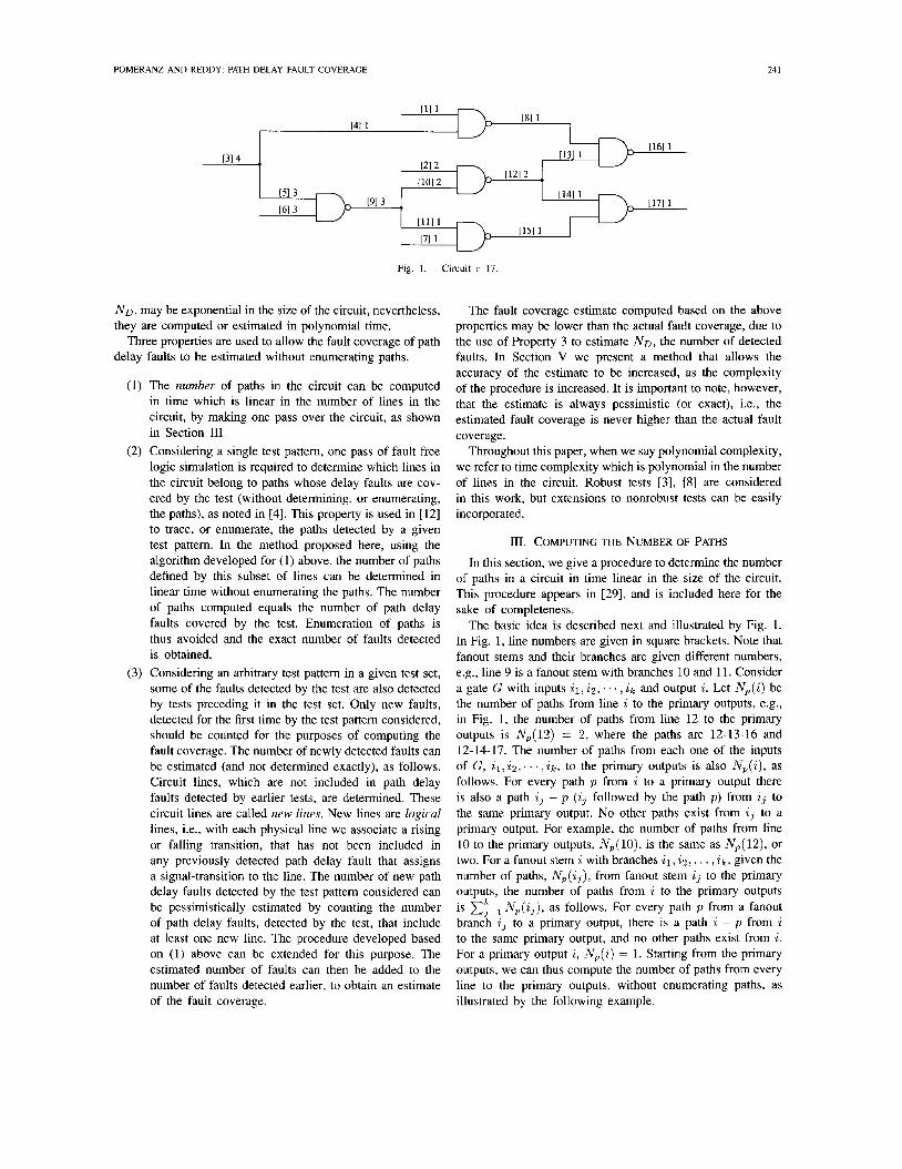
Fig. 1. Circuit c 17.

N D , may be exponential in the size of the circuit, nevertheless, they are computed or estimated in polynomial time.

Three properties are used to allow the fault coverage of path faults to be estimated without enumerating paths.

The number of paths in the circuit can be computed in time which is linear in the number of lines in the circuit, by making one pass over the circuit, as shown in Section I11 Considering a single test pattern, one pass of fault free logic simulation is required to determine which lines in the circuit belong to paths whose delay faults are covered by the test (without determining, or enumerating, the paths), as noted in [4]. This property is used in [12] to trace, or enumerate, the paths detected by a given test pattern. In the method proposed here, using the algorithm developed for (1) above, the number of paths defined by this subset of lines can be determined in linear time without enumerating the paths. The number of paths computed equals the number of path delay faults covered by the test. Enumeration of paths is thus avoided and the exact number of faults detected is obtained. Considering an arbitrary test pattern in a given test set, some of the faults detected by the test are also detected by tests preceding it in the test set. Only new faults, detected for the first time by the test pattern considered, should be counted for the purposes of computing the fault coverage. The number of newly detected faults can be estimated (and not determined exactly), as follows. Circuit lines, which are not included in path delay faults detected by earlier tests, are determined. These circuit lines are called new lines. New lines are logical lines, i.e., with each physical line we associate a rising or falling transition, that has not been included in any previously detected path delay fault that assigns a signal-transition to the line. The number of new path delay faults detected by the test pattern considered can be pessimistically estimated by counting the number of path delay faults, detected by the test, that include at least one new line. The procedure developed based on (1) above can be extended for this purpose. The estimated number of faults can then be added to the number of faults detected earlier, to obtain an estimate of the fault coverage.

The fault coverage estimate computed based on the above properties may be lower than the actual fault coverage, due to the use of Property 3 to estimate N D , the number of detected faults. In Section V we present a method that allows the accuracy of the estimate to be increased, as the complexity of the procedure is increased. It is important to note, however, that the estimate is always pessimistic (or exact), i.e., the estimated fault coverage is never higher than the actual fault coverage.

Throughout this paper, when we say polynomial complexity, we refer to time complexity which is polynomial in the number of lines in the circuit. Robust tests [3], [SI are considered in this work, but extensions to nonrobust tests can be easily incorporated.

111. COMPUTING THE NUMBER OF PATHS

In this section, we give a procedure to determine the number of paths in a circuit in time linear in the size of the circuit. This procedure appears in [29], and is included here for the sake of completeness.

The basic idea is described next and illustrated by Fig. 1. In Fig. 1, line numbers are given in square brackets. Note that fanout stems and their branches are given different numbers, e.g., line 9 is a fanout stem with branches 10 and 11. Consider a gate G with inputs i l , i2, . . . , i k and output i. Let Np(i) be the number of paths from line i to the primary outputs, e.g., in Fig. 1, the number of paths from line 12 to the primary outputs is Np(12) = 2, where the paths are 12-13-16 and 12-14-17. The number of paths from each one of the inputs of G, i 1 , i 2 , . . . , i k , to the primary outputs is also Np( i ) , as follows. For every path p from i to a primary output there is also a path i j - p ( i j followed by the path p ) from ij to the same primary output. No other paths exist from i j to a primary output. For example, the number of paths from line 10 to the primary outputs, Np(lO), is the same as Np(12), or two. For a fanout stem i with branches i l , i 2 , . . . , i k , given the number of paths, N p ( i j ) , from fanout stem ij to the primary outputs, the number of paths from i to the primary outputs is E:=, Np( i j ) , as follows. For every path p from a fanout branch i, to a primary output, there is a path i - p from i to the same primary output, and no other paths exist from i . For a primary output i , Np(i) = 1. Starting from the primary outputs, we can thus compute the number of paths from every line to the primary outputs, without enumerating paths, as illustrated by the following example.


[16] 1x0 (8)

[121 111 Cl ooo

1101 0x1 (9)

[3] 111

[17] 0x1 (15) [5] 111

PI 0x1 (6) ,, [61 1x0 (6)

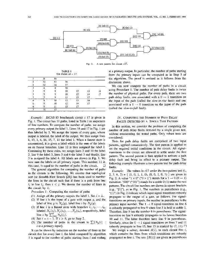
Fig. 2. A test pattern for circuit cl7.

TABLE I THE PATHS OF c 17

1 8 16 2 12 13 16

3 4 8 16 3 5 9 10 12 13 16 3 5 9 10 12 14 17 3 5 9 11 15 17 6 9 10 12 13 16 6 9 10 12 14 17 6 9 11 15 17 7 15 17

at a primary output. In particular, the number of paths starting from the primary inputs can be computed as in Step 5 of the algorithm. The proof is omitted as it follows from the discussion above.

We can now compute the number of paths in a circuit using Procedure 1. The number of path delay faults is twice the number of physical paths. For every path, there are two path delay faults, one associated with a 0 + 1 transition on the input of the path (called the slow-to-rise fault) and one associated with a 1 -+ 0 transition on the input of the path (called the slow-to-fall fault).

Example: ISCAS-85 benchmark circuit c 17 is given in Fig. 1. The circuit has 11 paths, listed in Table I as sequences of line numbers. To compute the number of paths, we assign every primary output the label 1. Lines 16 and 17 in Fig. 1 are thus labeled by 1. We assign the inputs of every gate, whose output is labeled, the label of the output. We thus assign lines 8, 13, 1, 4, 14, 15, 7, 11 the label 1. When a fanout stem is encountered, it is given a label which is the sum of the labels on its fanout branches. Line 12 is thus assigned the label 2. Continuing by these rules, we assign lines 2 and 10 the label 2, line 9 the label 3, lines 5 and 6 the label 3 and finally, line 3 is assigned the label 4. All labels are shown in Fig. 1. We now sum the labels on all primary inputs. This number, 11 in this case, is equal to the number of paths in the circuit. 0

The general algorithm for computing the number of paths in the circuits is the following. We assume that topological sort (or Breadth First Search [28]) has been used to number the lines in the circuit such that if there is a path from line li to line Zj, then i < j . We denote the number of lines in the circuit by L.

Procedure I : Computing the number of paths (1) Assign all the primary outputs the label 1. Set i = L. (2) If line i is the input of a gate with output g, and the

label of line g is N p ( g ) , label line i by N p ( g ) . (3) If line i is a fanout stem with branches i1, iz; . . . , i k ,

labeled N p ( i l ) , N p ( i z ) , . . . , Np( ik ) , respectively, label line i by ~ ~ = l N p ( i j ) .

(4) Set i = i - 1. If i > 0, go to Step 2. (5) The number of paths in the circuit is C { N p ( i ) :

It can be shown by induction on the number of lines in the circuit that for every line 1, the label computed by algorithm 1 is equal to the number of paths starting from 1 and ending

i is a primary input}.

Iv . COMPUTING THE NUMBER OF PATH DELAY FAULTS DETECTED BY A SINGLE TEST PAITERN

In this section, we consider the problem of computing the number of path delay faults detected by a single given test, without enumerating the tested paths. Only robust tests are considered.

Tests for path delay faults are comprised of two input patterns, applied consecutively. The first pattern is applied to set the required initial conditions in the circuit. All signal- transitions in the circuit are allowed to settle under the first pattern. The second pattern is then applied to activate a path delay fault and bring its effect to a primary output. The following example illustrates a two-pattern test for path delay faults.

Example: The values in c17 under the two-pattern test (1, 2, 3, 6, 7) = ( (1, 0, 1, 1, 0), (0, 0, 1, 0, 1) ) are given in Fig. 2. A value “1 x 0” (“0 x 1”) stands for a 1 -+ 0 (0 --+ 1) transition. “000” (“1 11”) stands for a stable 0 (1) under the two patterns. The circuit line numbers are shown in square brackets (e.g., “[l]”), as in Fig. 1. The numbers in parentheses (e.g., “( 1)”) in Fig. 2 indicate which input signal-transitions robustly propagate to the output of a gate, as follows. For signal- transitions on primary inputs, the number in parentheses is the primary input number. The 1 --+ 0 signal-transition on line 6 is robustly propagated to line 9 when line 5 is held at stable 1. Therefore, line 9 has the number 6 in parentheses. The signal- transition on line 9 robustly propagates to its fanout branches 10 and 11. The latter therefore have line 9 in parentheses. Similarly, since the 0 -+ 1 signal-transitions on lines 7 and 11 robustly propagate to line 15, line 15 is marked by (7, 11). 0

We assign a subset, denoted R(i), to each circuit line i , which contains the lines from which transitions are robustly propagated to line i . The sets {R( i )} are given in parentheses

POMERANZ AND REDDY: PATH DELAY FAULT COVERAGE 243

I310 ., [I61 1

P I 0

no1 0

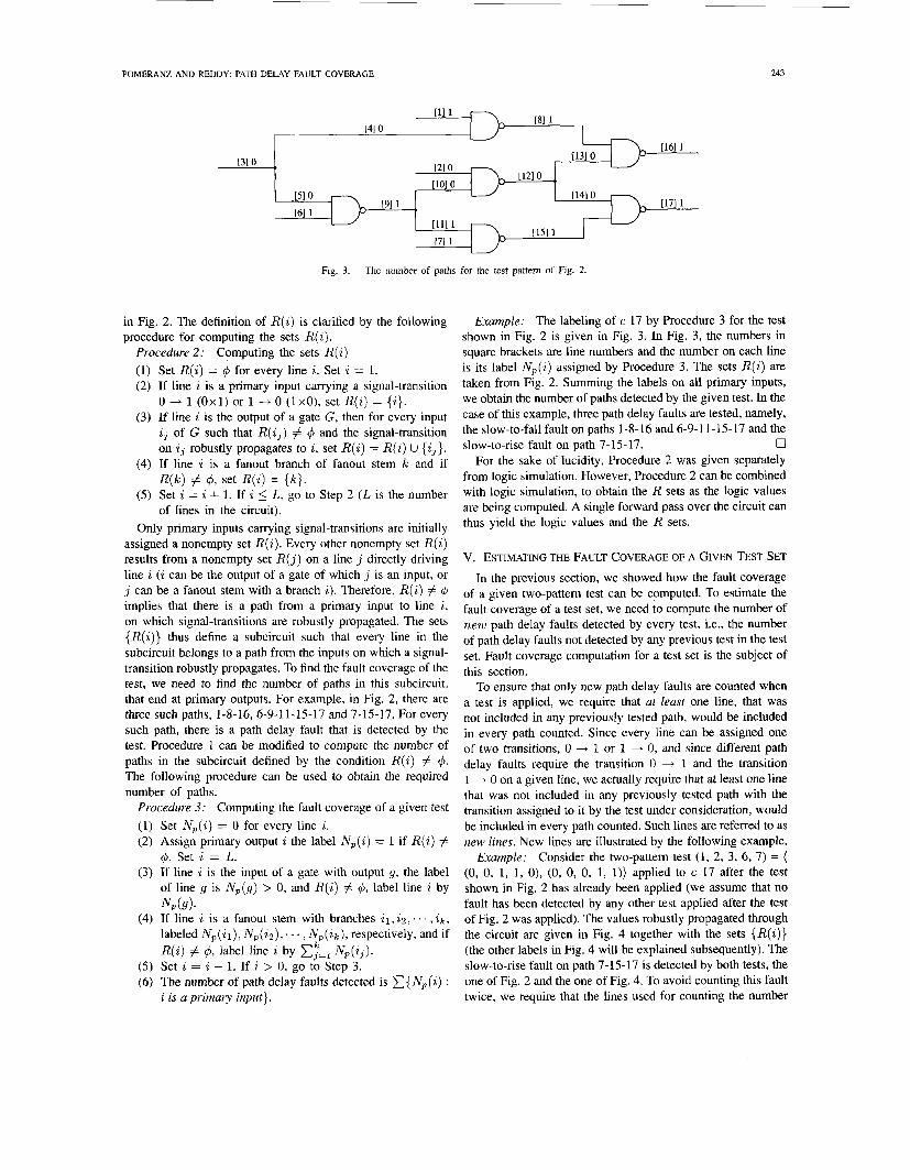
in Fig. 2. The definition of R(i) is clarified by the following procedure for computing the sets R( 2).

Computing the sets R(i) Procedure 2: (1) Set R(i) = $I for every line i. Set i = 1. (2) If line i is a primary input carrying a signal-transition

0 4 1 (0x1) or 1 -+ 0 (IxO), set R(i) = { i } . (3) If line i is the output of a gate G, then for every input

i, of G such that R( i3 ) # 4 and the signal-transition on Z, robustly propagates to i , set R(i) = R(i) U {i,}.

(4) If line i is a fanout branch of fanout stem k and if R(k) # $I, set R(i) = { k } .

(5) Set i = i + 1. If i 5 L, go to Step 2 ( L is the number of lines in the circuit).

Only primary inputs carrying signal-transitions are initially assigned a nonempty set R(i). Every other nonempty set R(i) results from a nonempty set R( j ) on a line j directly driving line i ( i can be the output of a gate of which j is an input, or j can be a fanout stem with a branch i ) . Therefore, R(i) # $ implies that there is a path from a primary input to line i , on which signal-transitions are robustly propagated. The sets {R( i )} thus define a subcircuit such that every line in the subcircuit belongs to a path from the inputs on which a signal- transition robustly propagates. To find the fault coverage of the test, we need to find the number of paths in this subcircuit, that end at primary outputs. For example, in Fig. 2, there are three such paths, 1-8-16, 6-9-1 1-15-17 and 7-15-17. For every such path, there is a path delay fault that is detected by the test. Procedure 1 can be modified to compute the number of paths in the subcircuit defined by the condition R(i) # 4. The following procedure can be used to obtain the required number of paths.

Procedure 3: Computing the fault coverage of a given test Set Np( i ) = 0 for every line i . Assign primary output i the label N p ( i ) = 1 if R(i) # 4. Set i = L. If line i is the input of a gate with output g, the label of line g is N p ( g ) > 0, and R(i) # 4, label line i by

If line i is a fanout stem with branches i l , Z z , . . . , i k ,

labeled Np( i l ) , Np(ip) , . . . , Np( ik ) , respectively, and if R(i) # 4, label line i by E$=, N p ( i J ) . Set i = i - 1. If i > 0, go to Step 3. The number of path delay faults detected is E { N p ( i ) :

N p ( g ) .

Example: The labeling of c 17 by Procedure 3 for the test shown in Fig. 2 is given in Fig. 3. In Fig. 3, the numbers in square brackets are line numbers and the number on each line is its label N p ( i ) assigned by Procedure 3. The sets R(z) are taken from Fig. 2. Summing the labels on all primary inputs, we obtain the number of paths detected by the given test. In the case of this example, three path delay faults are tested, namely, the slow-to-fall fault on paths 1-8-16 and 6-9-11-15-17 and the

0 For the sake of lucidity, Procedure 2 was given separately

from logic simulation. However, Procedure 2 can be combined with logic simulation, to obtain the R sets as the logic values are being computed. A single forward pass over the circuit can thus yield the logic values and the R sets.

slow-to-rise fault on path 7-15-17.

v. ESTIMATING THE FAULT COVERAGE OF A GIVEN TEST SET

In the previous section, we showed how the fault coverage of a given two-pattern test can be computed. To estimate the fault coverage of a test set, we need to compute the number of new path delay faults detected by every test, i.e., the number of path delay faults not detected by any previous test in the test set. Fault coverage computation for a test set is the subject of this section.

To ensure that only new path delay faults are counted when a test is applied, we require that at least one line, that was not included in any previously tested path, would be included in every path counted. Since every line can be assigned one of two transitions, 0 --t 1 or 1 + 0, and since different path delay faults require the transition 0 + 1 and the transition 1 ---f 0 on a given line, we actually require that at least one line that was not included in any previously tested path with the transition assigned to it by the test under consideration, would be included in every path counted. Such lines are referred to as new lines. New lines are illustrated by the following example.

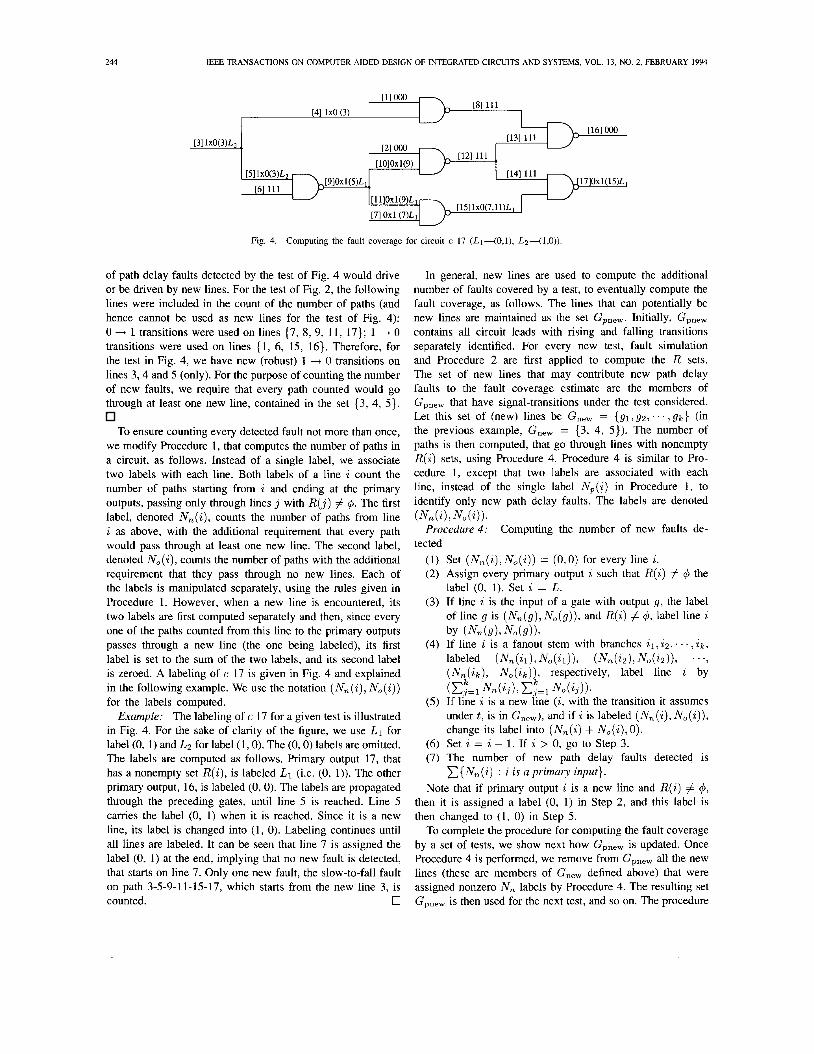
Consider the two-pattern test (1, 2, 3, 6, 7) = ( (0, 0, 1, 1, 0), (0, 0, 0, 1, 1)) applied to c 17 after the test shown in Fig. 2 has already been applied (we assume that no fault has been detected by any other test applied after the test of Fig. 2 was applied). The values robustly propagated through the circuit are given in Fig. 4 together with the sets {R( i )} (the other labels in Fig. 4 will be explained subsequently). The slow-to-rise fault on path 7-15-17 is detected by both tests, the one of Fig. 2 and the one of Fig. 4. To avoid counting this fault twice. we reauire that the lines used for counting the number

Example:

i is a primary input}. -


[8] 111 [11 coo

PI 1x0 (3)

MI OOO

[121 111 PI coo

[1OIOx1(9)

[311XO(3)L2

[9]OX1(5)LL 17IOx1(15)L, [511Xo(3)Lz

[6] 111

Fig. 4. Computing the fault coverage for circuit c 17 (Ll-(O,l), Lz-(l,O)).

of path delay faults detected by the test of Fig. 4 would drive or be driven by new lines. For the test of Fig. 2, the following lines were included in the count of the number of paths (and hence cannot be used as new lines for the test of Fig. 4): 0 -+ 1 transitions were used on lines (7, 8, 9, 11, 17); 1 + 0 transitions were used on lines { 1, 6, 15, 16). Therefore, for the test in Fig. 4, we have new (robust) 1 + 0 transitions on lines 3 , 4 and 5 (only). For the purpose of counting the number of new faults, we require that every path counted would go through at least one new line, contained in the set (3, 4, 5 ) .

To ensure counting every detected fault not more than once, we modify Procedure 1, that computes the number of paths in a circuit, as follows. Instead of a single label, we associate two labels with each line. Both labels of a line i count the number of paths starting from i and ending at the primary outputs, passing only through lines j with R( j ) # 4. The first label, denoted N,(i) , counts the number of paths from line i as above, with the additional requirement that every path would pass through at least one new line. The second label, denoted No(i ) , counts the number of paths with the additional requirement that they pass through no new lines. Each of the labels is manipulated separately, using the rules given in Procedure 1. However, when a new line is encountered, its two labels are first computed separately and then, since every one of the paths counted from this line to the primary outputs passes through a new line (the one being labeled), its first label is set to the sum of the two labels, and its second label is zeroed. A labeling of c 17 is given in Fig. 4 and explained in the following example. We use the notation ( N , (i) , No( i)) for the labels computed.

Example: The labeling of c 17 for a given test is illustrated in Fig. 4. For the sake of clarity of the figure, we use L1 for label (0, 1) and Lz for label (1,O). The (0 ,O) labels are omitted. The labels are computed as follows. Primary output 17, that has a nonempty set R(z), is labeled L1 (i.e. (0, 1)). The other primary output, 16, is labeled (0, 0). The labels are propagated through the preceding gates, until line 5 is reached. Line 5 carries the label (0, 1) when it is reached. Since it is a new line, its label is changed into (1, 0). Labeling continues until all lines are labeled. It can be seen that line 7 is assigned the label (0, 1) at the end, implying that no new fault is detected, that starts on line 7. Only one new fault, the slow-to-fall fault on path 3-5-9-11-15-17, which starts from the new line 3, is counted. 0

In general, new lines are used to compute the additional number of faults covered by a test, to eventually compute the fault coverage, as follows. The lines that can potentially be new lines are maintained as the set Gpne,. Initially, Gpnew contains all circuit leads with rising and falling transitions separately identified. For every new test, fault simulation and Procedure 2 are first applied to compute the R sets. The set of new lines that may contribute new path delay faults to the fault coverage estimate are the members of Gpnew that have signal-transitions under the test considered. Let this set of (new) lines be G,,, = { g l , g z , . . . ,gk} (in the previous example, G,,, = (3, 4, 5)). The number of paths is then computed, that go through lines with nonempty R(i) sets, using Procedure 4. Procedure 4 is similar to Pro- cedure 1, except that two labels are associated with each line, instead of the single label N p ( i ) in Procedure 1, to identify only new path delay faults. The labels are denoted

Computing the number of new faults de- (Nn( i ) , N O ( 4 ) .

Procedure4:

(1) Set (Nn( i ) .No( i ) ) = (0,O) for every line i . ( 2 ) Assign every primary output i such that R(i) # 4 the

label (0, 1). Set i = L. (3) If line i is the input of a gate with output g , the label

of line g is (N,(g), N , ( g ) ) , and R(i) # 4, label line i

(4) If line i is a fanout stem with branches 21, i p , . . . , z k ,

labeled (N,(Zl). No( i l ) ) , (Nn(i2), No(i2)), . . ., ( N n ( i k ) , No(ik) ) , respectively, label line i by

(5 ) If line i is a new line ( i , with the transition it assumes under t , is in G,,,), and if i is labeled (N,(i), No(z)), change its label into (N, ( i ) + No(i ) , 0).

(6) Set i = i - 1. If i > 0, go to Step 3. (7) The number of new path delay faults detected is

Note that if primary output i is a new line and R(i) # 4, then it is assigned a label (0, 1) in Step 2, and this label is then changed to (1, 0) in Step 5.

To complete the procedure for computing the fault coverage by a set of tests, we show next how Gpnew is updated. Once Procedure 4 is performed, we remove from Gpnew all the new lines (these are members of G,,, defined above) that were assigned nonzero N, labels by Procedure 4. The resulting set Gpnew is then used for the next test, and so on. The procedure

tected

by (Nn(g), No(g)).

IC (E,"=, Nn( iJ ) , C,=l N O ( i J ) ) .

{ N , ( i ) : i is a primary input).


for computing the fault coverage of a given test set, T , is given next.

Procedure 5: Estimating the fault coverage of a given test set

(1) Set Gpnew to include every line in the circuit, with a rising and a falling transition on every line. Set ND = 0 ( N o is used to count the number of faults detected).

(2) Select a test t from T. Apply fault simulation and Procedure 2 to obtain the sets { R(i) 1 for t . Set G,,, =

(3) Apply Procedure 4 to compute the number of new faults detected under t and add this number to N o .

(4) For every line j in the circuit, if j , with the transition it assumes under t , is in G,,,, and N , ( j ) # 0, remove j with the corresponding transition from Gpnew.

Gpnew n ( j R( j ) # 4) .

(5) Set T = T - { t ). If T # 4, go to Step 2. (6) N D is the number of faults detected by T . To compute

the fault coverage, apply Procedure 1 to compute the number of paths N p and the number of faults, N p = 2 . N p . The fault coverage is 2.

It is important to note that new path delay faults can be covered by a test even when no new lines exist that carry new transitions under the test considered. The following example illustrates such a case.

Consider the circuit shown in Fig. 5. Suppose that the first test applied to the circuit assigns the following values to the primary inputs. 1-021, 4-021, 6-000, 11-021, 13-000. The test detects the slow-to-rise faults on paths 1-2- 5-8-9-12-15,4-5-8-9-12-15 and 11-12-15, and leaves lines (3, 6, 7, 10, 13, 14) as new lines carrying rising transitions.

Suppose that the following test is applied to the circuit next. 1-021, 4-000, 6-021, 11-000, 13 - 0x1. The test detects the slow-to-rise faults on paths 1-3-7-8-10-14-15, 6-7-8-10-14-15 and 13-14-15, and leaves no new lines carrying rising transitions. As a result, no additional faults with rising transitions can be detected. However, the rising transitions along the following paths have not been tested yet. 1-2-5-8-10-14-15, 4-5-8-10-14-15, 1-3-7-8-9-12-15 and 6-7-8-9- 12-15. Tests to detect these faults exist, as follows. The test 1-021, 4-021, 6-000, 11-000, 13-021 detects the first two faults, and the test 1-021, 4-000, 6-021, 11-0x1, 13-000 detects the last two faults. However, even if these tests are applied, the count of the number of tested faults will not increase, since no new lines exist on these paths, that carry rising transitions. 0

The previous example shows that the fault coverage estimate may be pessimistic. We refer to the approximation described above as the zero-order approximation. To increase the quality of the fault coverage estimate based on new lines, we next propose to divide the circuit into subcircuits, such that each subcircuit has a unique set of paths contained in it. We then consider new lines with respect to each subcircuit separately, to increase the accuracy of the estimate, as follows.

We find a cut through the circuit, such that every path from inputs to outputs passes through exactly one line in the cut. Let c = {cl, c2. . . . , ck) be such a cut. A simple way to select C is to select all primary inputs or all primary outputs. In our experiments, the cut that includes primary inputs or

Example:

all the fanout branches of a primary input when the primary input is a fanout stem, and the cut that includes the inputs of all gates whose outputs are primary outputs, were considered. The larger of the two cuts was used. Consider the following example.

Example: For c 17, C1 = { 1, 2, 3, 6, 7) is a cut such that every path from inputs to outputs passes through exactly one line in Cl, since C1 includes all primary inputs. Cz = { 16, 17) is another such cut, since it includes all primary outputs. We can increase the size of C1 by replacing input 3 by its fanout branches, to obtain C, = { 1, 2, 4, 5, 6, 7). Similarly, we can increase the size of C2 by replacing each primary output by the inputs of the gate directly driving it, to obtain C, = (8, 13, 14, 15). The advantages of selecting a larger cut will become clear later. The cut C, = { 1, 4, 9) is not suitable, since there is a path from input 7 to output 17 that does not pass through this cut. 0

We use the cut C to divide the circuit into subcircuits, each one containing a disjoint set of paths, as follows. For every c, E C , we define a subcircuit that inludes every line g such that there is a path in the circuit from g to c, or from c, to g. The following example illustrates this division.

Consider c 17 and the cut C = { 1, 2, 4, 5, 6, 7). The subcircuit for line 1 includes the lines { 1, 8, 16); the subcircuit for line 2 includes the lines ( 2 , 12, 13, 14, 16, 17); the subcircuit for line 4 includes the lines (3, 4, 8, 16); the subcircuit for line 5 includes the lines (3, 5, 9, 10, 11, 12, 13, 14, 15, 16, 17); the subcircuit for line 6 includes the lines (6, 9, 10, 11, 12, 13, 14, 15, 16, 17); and the subcircuit for line 7 includes the lines (7, 15, 17). Each one of these subcircuits contains a unique set of paths from inputs to outputs, none of

0 Since every subcircuit contains a unique line c, of the cut G,

every path in that subcircuit must pass through e,. The sets of paths contained in different subcircuits are therefore disjoint, and for computing the fault coverage of a test, we can count the number of new path delay faults detected in each subcircuit separately and then add the numbers. For every subcircuit separately, we record all the lines and signal-transitions used in the fault coverage estimate for previous tests. A line that is not new in the subcircuit of a line c1 E C may thus be new in the subcircuit of a line c2 E C, and may still be useful in improving the fault coverage estimate. This method is referred to as the first-order approximation, since the division of the circuit into subcircuits is determined by a single cut.

Comparing the first-order approximation to the zero-order approximation, where all previously used lines and signal- transitions are recorded together, the first-order estimate is higher and more accurate. Comparing the complexity of the two approaches, the number of computations required by the zero-order approximation is approximately multiplied by the size of the cut in the case of the first-order approximation (similar computations are performed for each subcircuit, however, they are performed for IC1 subcircuits in the case of the first-order approximation, instead of a single one in the case of the zero-order approximation).

It is possible to further improve the accuracy of the estimate by considering two cuts instead of one, to obtain a second-

Example:

which is included in any other subcircuit.

-


order approximation. For two cuts C1 and (72, ICI~ . IC21

subcircuits are considered, each one with its own set of new lines. Some of the subcircuits may be empty, and need not be considered, e.g., for c 17 with G1 = {I, 2, 3 , 6, 7) and C2 = (16, 17}, lines 1 and 17 define an empty subcircuit, since there is no path from line 1 to line 17. The Icth-order approximation uses Ic cuts, and its complexity is O(L'+') per test, where L is the number of lines in the circuit. This can be seen as follows. For every test and every subcircuit, the additional fault coverage is computed by performing a constant number of passes over the circuit (three passes: the first for logic simulation and computing the sets R(i), the second for computing the number of new path delay faults detected, and the third for updating the new lines). The complexity of each pass is O(L) . The size of every cut is also O ( L ) , therefore, the number of subcircuits is O(Lk) . The total complexity follows.

Using the procedures above, it is also possible to restrict the computation only to the longest paths. For this purpose, we label each line by its maximum distance (in lines or in gate delays) from the primary inputs. A single forward pass allows such a labeling, as follows. Denoting the maximum distance of line i from the primary inputs by d ( i ) , if line i is an output of a gate with inputs 21, . . . , i k , and assuming that the distances of i l , . . . , 2' are known, the distance of line i is computed as max(d(i,)} + 1. Gate delays can also be accommodated,

by using max{d(i,)} + A(i), where A(i) is the delay of the

gate. For a fanout stem i with branches 21, . . . , i,, the branches are labeled by d ( i ) + A(i), where again, A(i) depends on the delay model (A(i) may be zero if the delay of a line is neglected). For the primary inputs, d(z) = 0. The d labels can thus be computed by a single forward pass, using the rules above. Once the d labels are computed, a single backward pass can be used to mark all the lines contributing to longest paths, as follows. All primary outputs are marked. Input i, of a gate with output i is marked if d ( i ) = d( i , ) + A(i), i.e., i, determined the maximum distance for line i. Similarly, fanout stems are marked. The procedures developed above for estimating the fault coverage are then applied only to the lines marked, belonging to longest paths.

The following property of the computed fault coverage estimates deserves attention. The estimated fault coverage of a single two-pattern test, or of the first test that detects any fault in a test set, is exact. Based on this observation, we present in Section VI1 an improvement of the basic scheme proposed in this section that increases the accuracy of the estimate by changing the order in which tests are evaluated.

23

Z J

VI. EXPERIMENTAL RESULTS

We applied the method proposed in this work to estimating the fault coverage in several sets of circuits. The results are reported in this section.

Two types of examples are considered, as follows. (1) To demonstrate the accuracy of the estimate obtained by nonenumerative simulation, we consider circuits where the number of faults detected is low. For such circuits, we use an accurate fault simulation procedure (described below) to obtain the exact number of faults detected, and compare it

with the estimate obtained by the proposed nonenumerative method. ( 2 ) To demonstrate the effectiveness of nonenumerative simulation, we consider circuits where the number of faults detected is too large to apply an accurate fault simulation procedure. For such circuits, we report the run times of the nonenumerative procedure, and show how enormous numbers of paths can be simulated in reasonable times.

The accurate fault simulation procedure we used for comparison purposes has the following features. It uses the path representation scheme from [29] to assign a unique integer index to each path. As a result, storage of detected faults requires that a single integer and a transition (rising or falling) be stored for every fault. In addition, comparison of a newly detected fault with the already detected faults, to determine if the fault should be stored, or it has already been detected by a previous test, requires simple integer comparison (as opposed to comparison of sequences of gate numbers if the complete paths are stored). The index of a path is determined as a sum of labels assigned to its lines. A simple labeling procedure, based on Procedure 1, is described in [29] to assign the labels to all the lines in the circuit. The fault simulation procedure is similar to Procedure 2, except that instead of the sets R(i), path indices are computed. Before presenting the procedure, we introduce the following notation. The label for path representation assigned to line i is denoted by M(i ) . The total number of paths in the circuit is denoted by N p . Each path is assigned an index between 0 and Np - 1. To distinguish between paths with rising and falling transitions, we use 0,1, . . . , Np - 1 as path indices when the paths carry rising transitions, and we use N p , Np + 1, . . . . 2Np - 1 as path indices when the paths carry falling transitions. The fault simulation procedure is as follows.

Procedure 6: Accurate fault simulation (1) Set D ( i ) = q5 for every line i . Set i = 1. (2) If line i is a primary input carrying a signal-transition

O + 1 (0 x I), set D(i ) = { M ( i ) } . If line i is a primary input carrying a signal-transition 1 --+ 0 (1 x 0), set D ( i ) = { M ( i ) + N p } .

( 3 ) If line i is the output of a gate G, then for every input i, of G such that D ( i J ) # 4 and the signal-transition on i, robustly propagates to i , set D(i ) = D ( i ) U {d+ M ( i ) : d E D(i,)}.

(4) If line i is a fanout branch of fanout stem k and if D(k) # 4, set D(i ) = { d + M ( i ) : d E D(Ic)}.

(5) Set i = i + 1. If i 5 L , go to Step 2 ( L is the number of lines in the circuit).

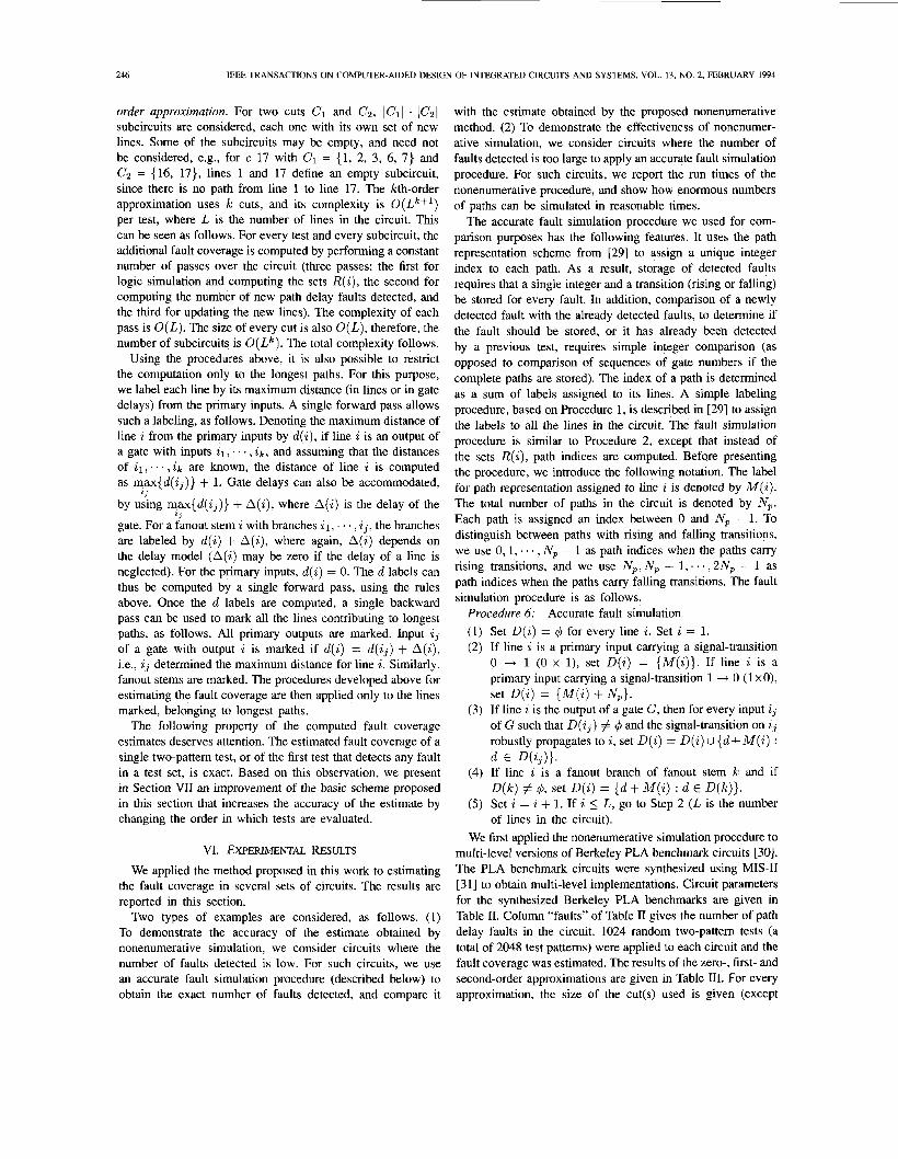
We first applied the nonenumerative simulation procedure to multi-level versions of Berkeley PLA benchmark circuits [30]. The PLA benchmark circuits were synthesized using MIS-I1 [ 3 11 to obtain multi-level implementations. Circuit parameters for the synthesized Berkeley PLA benchmarks are given in Table 11. Column "faults" of Table I1 gives the number of path delay faults in the circuit. 1024 random two-pattern tests (a total of 2048 test patterns) were applied to each circuit and the fault coverage was estimated. The results of the zero-, first- and second-order approximations are given in Table 111. For every approximation, the size of the cut(s) used is given (except


circuit Z9sym add6 adr4 alu 1 alu2 a h 3 col4 dk17 dk27 dk48 mish radd rckl rd53

xldn x9dn

vg2

24

TABLE I1 CIRCUT PARAMETERS-BERKELEY PLA’S

TABLE IV EXPERIMENTAL RESULTS FOR BERKELEY PLA,s-A DETERMINISTIC TEST SET

inp out lines faults 9 1 438 644 12 7 229 498 8 5 147 210 12 8 85 76 10 8 189 260 10 8 218 282 14 1 145 144 10 11 168 340 8 9 78 128 15 17 194 572 94 34 215 280 8 5 121 170 32 7 338 476 5 3 134 154

25 8 185 492 27 6 186 440 27 7 203 612 7 4 125 190

TABLE 111 EXPERIMENTAL RESULTS FOR BERKELEY PLAS-1024 RANDOM TESTS

Cut size, detected faults

circuit first second exact

Z9sym 644 19 77 19 77, 4 19 19 add6 498 157 47 233 47,15 233 233 adr4 210 108 27 162 27,ll 163 163 alu 1 76 76 28 76 28,21 76 76 a h 2 260 141 44 160 44.22 160 160 alu3 282 142 49 169 49.18 171 171 col4 144 0 46 0 46.2 0 0

faults zero

cut size, detected faults circuit zero first second exact Z9sym 420 77 644 644 add6 227 47 437 47. 15 498 498 adr4 139 27 208 27, 11 210 210 alul 76 28 76 76 a h 2 212 44 260 260 alu3 230 49 279 49, 18 282 282 col4 131 46 144 144 dk17 242 40 333 40, 24 340 340 dk27 100 23 128 128

569 46, 50 572 572 dk48 383 50 mish 265 114 279 114, 75 280 280 radd 1 07 26 159 26, 10 170 170 rckl 409 123 476 476 rd53 125 29 154 154

468 65, 12 492 492 vg2 320 65 xldn 308 68 421 68, 9 440 440 x9dn 417 58 588 58, 11 612 612

186 28, 9 190 190 24 1 I6 28

TABLE V EXPERIMENTAL RESULTS FOR 1024 RANDOM TESTS-ISCAS-85

cut size, detected faults

circuit zero first exact

c880 17284 354 222 394 394 c1355 8 346 432 5 208 5 5 c3540 57 353 344 369 306 397 397 c6288 197.886 E18 34 512 35 35

faults

dk17 340 108 40 122 4024 122 122 of paths, whereas the circuit has only 249 paths. Clearly, some dk27 12’ 62 23 83 237 21 83 83 of the subsets of paths are empty, as noted in Section V. dk48 572 0 50 0 46,50 0 0 Results for ISCAS-85 benchmark circuits are given in Table mish 280 228 114 253 114,75 255 255 radd 170 89 26 141 26.10 145 145 V. Except for c880, we include results only for circuits that rckl 476 58 123 66 123,15 66 66 have ve& large numbers of paths. Results-for fully scanned rd53 154 115 29 140 29, 8 140 140 ISCAS-89 circuits are given in Table VI. Note that 1024 vg2 492 94 65 164 65912 random tests may be too few to detect any significant number xldn 440 87 68 130 68,9 131 131 x9dn 612 84 58 15 58.11 117 117 of path delay faults (even stuck-at faults require larger numbers z4 190 102 28 153 28, 9 153 153

for the zero-order approximation, where the cut size is zero), followed by the number of path delay faults detected by 1024 random tests. Also included in Table 111 is the number of paths detected using accurate fault simulation. It can be seen that while the zero-order approximation gives results which are far from the exact numbers, the first order approximation deviates from the exact numbers by 1% on the average. The second order approximation gives exact numbers. Similar results are obtained when a deterministic test set, that detects all path delay faults, is used, as reported in Table IV. In Table IV, the results of the second-order approximation are omitted when the first-order approximation gives the exact numbers of detected faults.

For the second-order approximation as reported in Tables I11 and IV, the number of paths in some of the circuits is smaller than the number of subsets of paths defined by the cuts used, e.g., for add6, two cuts of sizes 47 and 15 define 705 subsets

of random tests), however, this number is large enough to show the applicability and accuracy of the estimate, that does not require path enumeration.

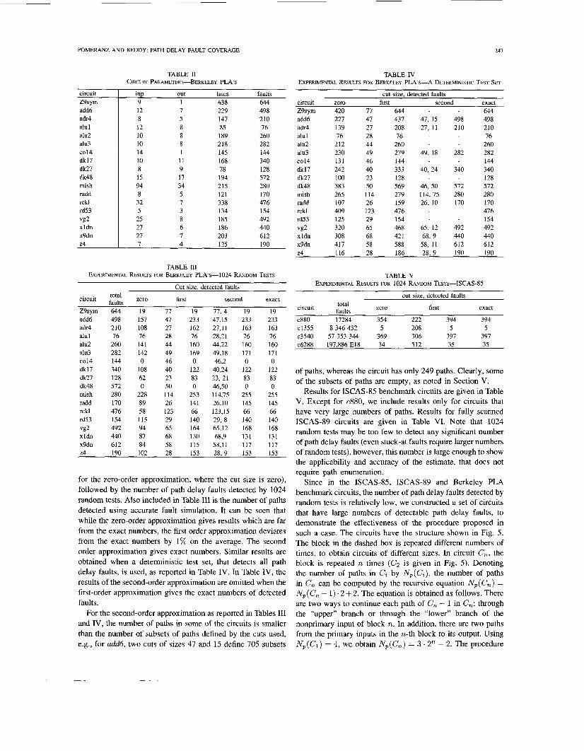
Since in the ISCAS-85, ISCAS-89 and Berkeley PLA benchmark circuits, the number of path delay faults detected by random tests is relatively low, we constructed a set of circuits that have large numbers of detectable path delay faults, to demonstrate the effectiveness of the procedure proposed in such a case. The circuits have the structure shown in Fig. 5. The block in the dashed box is repeated different numbers of times, to obtain circuits of different sizes. In circuit C,, the block is repeated n times (C, is given in Fig. 5). Denoting the number of paths in Ci by N,(Ci), the number of paths in C, can be computed by the recursive equation N,(C,) = Np( C, - 1) . 2 + 2. The equation is obtained as follows. There are two ways to continue each path of C, - 1 in C,: through the “upper” branch or through the “lower” branch of the nonprimary input of block n. In addition, there are two paths from the primary inputs in the n-th block to its output. Using Np(C1) = 4, we obtain Np(Cn) = 3 . 2 ” - 2. The procedure


TABLE VI EXPERIMENTAL RESULTS FOR 1024 RANDOM TESTS-ISCAS-89

cut size, detected faults

circuit inp out lines first exact

s27 7 4 26 56 33 7 44 44 s208 19 10 208 290 111 54 138 138 s298 17 20 298 462 259 85 271 271 s344 24 26 344 710 230 45 351 352 s349 24 26 349 730 231 46 351 352 s386 13 13 386 414 180 75 180 180 S 4 0 0 24 27 400 896 276 89 317 317 s420 35 18 420 738 163 102 211 211 S 4 4 4 24 27 444 1070 274 90 319 319 s510 25 13 510 738 337 91 448 448 s526 24 27 526 820 366 140 377 377 s64 1 54 43 640 3488 359 54 498 506 s713 54 42 713 43624 261 59 337 350 s820 23 24 820 984 341 282 341 341 s832 23 24 832 1012 338 288 338 338 s953 45 29 953 2266 398 115 575 575 s1196 32 31 1196 6194 461 201 554 554 s1238 32 31 1238 7116 478 222 577 577 s1423 91 79 1423 89452 891 255 1186 1222 s1488 14 25 1488 1924 600 281 649 649 s1494 14 25 1494 1952 602 283 651 651 s5378 214 228 5295 27084 2022 335 2319 2377 s9234 247 250 9234 489708 1386 644 1582 1585

faults zero

proposed was applied to a test set that detects all slow-to-fall path delay faults in the circuit. As many faults as possible were detected by every test, e.g., the test (1,4,6,11,13, . . .) = (lzO,111,111,111,111, 111,111,111,111~~ . .) detects all slow-to-fall delay faults on paths that start from input 1 (input numbers correspond to Fig. 5). Experimental results for several C, circuits are given in Table VII. The number of blocks in the circuit is given first, followed by the number of tests applied and the total number of path delay faults and the number of path delay faults detected. Time is given in the last column (time is measured in seconds on a SUN SPARC 2 Workstation). Floating-point numbers of double-accuracy had to be used to count the number of paths and the number of path delay faults detected.

VII. TEST ORDERING TO IMPROVE THE FAULT COVERAGE ESTIMATE ACCURACY

In this section, we consider an extension of the method proposed in the previous sections, with the aim of increasing the accuracy of the estimate. The method is based on ordering of the test set to reduce the loss of accuracy due to new faults that do not involve new lines. The test ordering scheme is matched to the approximation used for estimating the fault coverage, as explained below.

For a given test set, the fault coverage estimate obtained by the procedure proposed may depend on the order in which the tests are processed. Here, we do not refer to test ordering that changes the actual fault coverage of the test set. Rather, the test set is applied in its original order, and test ordering is used only to improve the fault coverage estimate. This is possible by regarding the test set as comprised of nonoverlapping two- pattern tests, i.e., for a test set T = ( t l , t z : . . . , t k ) , where

I I 1 I L - _ - - - - - - - - - - - - - - J L - - - - - - - - - - - - - - - - J

Fig. 5. Example circuits with exponential numbers of detectable faults.

TABLE VI1 RESULTS FOR THE CIRCUIT OF FIG. 5

n tests total faults detected faults time (s) 20 41 6 291 452 3 145 726 0.30 30 61 6 442 450 940 3 221 225 470 0.68 40 81 6 597 069 766 652 3 298 534 883 326 1.21 50 101 6 755 399 441 055 740 3 377 699 720 527 870 1.88

ti is a single input pattern, the two-pattern tests considered are ( t l , t z ) , ( t 2 , t 3 ) , ( t 3 , t ~ ) , . . . , ( t ~ - ~ , t k ) . In order to take advantage of this observation, the following property of the proposed estimation procedure is used to obtain an easy-to- implement heuristic to determine the order of processing of tests. The estimated fault coverage of a single two-pattern test, or of the first test that detects any fault in a test set, is exact. Based on this observation, we prefer to process tests that detect large numbers of faults at the beginning, so that more new lines would be available when they are evaluated, potentially increasing the fault coverage estimate.

Ordering for the zero-order approximation is performed as follows. First, the fault coverage of every test is obtained separately, i.e., as if it is the only test applied, using the zero- order approximation. The tests are then ordered by decreasing numbers of faults detected, and the fault coverage estimate for the test set is evaluated under the new order. More new lines are thus available when the tests that detect higher numbers of faults are evaluated. The procedure for ordering a test set T follows.

Procedure 7: Zero-order test ordering of a test set T (1) For every two-pattern test t E T , compute the number

of faults detected by t , N F ( ~ ) . Set To = () (To is the ordered test set, initially empty).

(2) Select a two-pattern test t’ E T with maximum N F ( ~ ’ ) . Set T = T - {t’} and To = To 0 (t’) (“0” denotes concatenation. In this step, t’ is added at the end of To).

( 3 ) If T # 4 , go to Step 2. Note that the computation of the number of faults detected

by a test t is independent of the number of faults in the circuit, therefore, the disadvantages of nonfault dropping fault simulation do not exist here. The complexity of Procedure 7 is thus lower than the complexity of evaluating the fault coverage of a given test set, since new lines do not have to be considered.

The test ordering of Procedure 7 can be used for any order of approximation. However, for the k-th order approximation, it may be advantageous to perform the test ordering for each subcircuit corresponding to a cut edge separately. The number of faults detected by every test is first computed, this time

POMERANZ AND REDDY: PATH DELAY FAULT COVERAGE

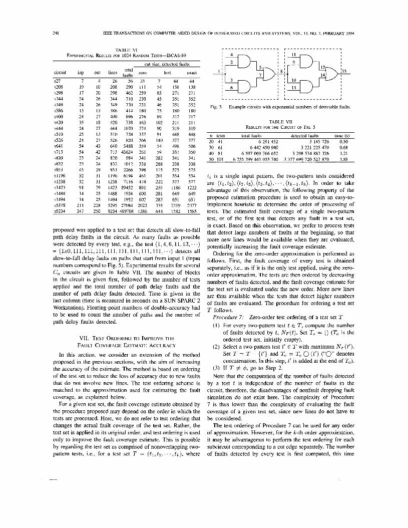
TABLE VI11 BERKELEY PLAT 1024 RANDOM TESTS

WITH TEST ORDERING BY ZERO-APPROXIMATION

cut size, detected faults circuit zero first exact Z9sym 19 77 19 19 add6 163 47 233 233 adr4 113 27 161 163 alu 1 76 28 76 76 ah2 143 44 160 160 ah3 143 49 169 171 col4 0 46 0 0 dk17 114 40 122 122 dk27 74 23 83 83 dk48 0 50 0 0 mish 233 114 253 255 radd 91 26 142 145 rckl 58 123 66 66 rd53 117 29 140 140 vg2 125 65 166 168 xldn 102 68 129 131 x9dn 90 58 115 117 24 109 28 153 153

using the k-th order approximation, in order to find the number of faults detected with respect to each subcircuit separately. The test set is then ordered for each cut edge separately, in order of decreasing number of detected faults. Although the complexity of test ordering is increased as IC is increased, its accuracy is also expected to be increased.

Results of application of test ordering are presented next. In Table VIII, results of using the zero-order approximation for test ordering for Berkeley PLA multi-level circuits is given. For the same test ordering, the zero- and first-order approximations were applied. The results should be compared to the results of Table 111, where no test ordering is employed. It can be seen that test ordering improves the results for the zero-order approximation significantly. The first-order approximation is highly accurate even without test ordering, and little improvement is obtained. For ISCAS-89 circuits, results of the zero-order approximation are given in Table IX, and should be compared with the results given in Table VI.

VIII. CONCLUSION

A method to estimate the coverage of path delay faults of a given test set, without enumerating paths, was proposed. The method was based on properties, that allow the number of path delay faults detected by a test to be computed in linear time. An approximation was required to estimate the fault coverage of a test set comprised of more than one test. Several levels of approximation, with increasing accuracy and increasing complexity, were proposed. In all cases, the method was polynomial in the number of lines in the circuit, and thus allows circuits with exorbitant numbers of paths to be considered under the path delay fault model. Experimental results were presented to show the effectiveness of the estimate in accurately evaluating the path delay fault coverage. A method to improve the estimates, based on test ordering, was also proposed.

249

TABLE IX ISCAS-89 1024 RANDOM TESTS WITH

TEST ORDERING BY ZERO-APPROXIMATION

exact detected zero-order circuit

s27 40 44 s208 124 138 s298 26 1 27 1 s344 240 352 s349 243 352 s386 180 180 s400 280 317 s420 185 21 1 s444 283 319 s5 IO 350 448 ~ 5 2 6 368 377 s641 385 506 s713 277 350 s820 341 341 s832 338 338 s953 470 575 S I 196 473 554 s 1238 497 577 s1423 96 1 1222 s1488 612 649 s1494 614 65 1 s5378 2033 2377 s9234 1396 1585

ACKNOWLEDGMENT

The authors would like to thank Prasanti Uppaluri of the University of Iowa for helping with the implementation of some of the programs used and for collecting the data reported in the paper.

REFERENCES

J. D. Lesser and J. J. Schedletsky, “An experimental delay test generator for LSI logic,”lEEE Trans. Comput., vol. C-29, pp. 235-248, Mar. 1980. Y. K. Malaiya and R. Narayanaswamy, “Testing for timing faults in synchronous sequential integrated circuits,” in Proc. Int. Test Conf, Oct. 1983, pp. 56G571. S. M. Reddy, M. K. Reddy, and V. D. Agrawal, “Robust tests for stuck- open faults in CMOS combinational logic circuits”, in Proc. Int. Symp. on Fault-Tolerant Computing, Florida, June 1984, pp. 4449. G. L. Smith, “Model for delay faults based upon paths,” in Proc. Int. Test Conf, Nov. 1985, pp. 342-349. K. D. Wagner, “The error latency of delay faults in combinational and sequential circuits,” in Proc. Int. Test Con$., Nov. 1985, pp. 334-341. J. Savir and W. H. McAnney, “Random pattern testability of delay faults,” in Proc. Int. Test Conf., Sept. 1986, pp. 263-273. C. J. Lin and S. M. Reddy, “On delay fault testing in logic circuits,” IEEE Trans. Computer-Aided Design, pp. 694-703, Sept. 1987. E. S. Park and M. R. Mercer, “Robust and nonrobust tests for path delay faults in a combinational logic,” in Proc. Int. Test Conf., Sept. 1987, pp. 1027-1034. S. M. Reddy, C. J. Lin, and S . Patil, “An automatic test pattern generator for the detection of path delay faults,” in Proc. Int. Con$. on Computer- Aided Design, Santa Clara, CA, Nov. 1987, pp. 284-287. S. Kundu and S . M. Reddy, “On the design of robust testable CMOS combinational logic circuits,” in Proc. Int. Symp. on Fault-Tolerant Computing, Tokyo, Japan, June 1988, pp. 220-225. S. Kundu, S. M. Reddy, and N. K. Jha, “On the design of robust multiple fault testable CMOS combinational logic circuits,” in Proc. Int. Conf. on Computer-Aided Design, Santa Clara, CA, Nov. 1988, pp. 24G243. M. H. Schultz, F. Fink, and K. Fuchs, “Parallel pattern fault simulation of path delay faults”, in Proc. Design Autom. Conf.., pp. 357-363, June 1989. M. H. Schultz, K. Fuchs and F. Fink, “Advanced automatic test pattern generation techniques for path delay faults’’, in Proc. Int. Symp. on Fault-Tolerant Computing, June 1989, pp. 44-51.

IEEE TRANSACTIONS ON COMPUTER-AIDED DESIGN OF INTEGRATED CIRCUITS AND SYSTEMS, VOL. 13, NO. 2, FEBRUARY 1994

S. Devadas, “Delay test generation for synchronous sequential circuits,” in Proc. Int. Test Con f , Washington, DC, Aug. 1989, pp. 144-152. K. Roy, K. De, J. A. Abraham, and S. Lusky, “Synthesis of delay fault testable combinational logic,” in Proc. Inr. Conf. on Computer-Aided Design, Santa Clara, CA, Nov. 1989, pp. 418421. N. K. Jha and S. Kundu, Testing and Reliable Design of CMOS Circuits . Norwell, MA: Kluwer, 1990. S. Devadas and K. Keutzer, “Necessary and sufficient conditions for robust delay-fault testability of combinational logic circuits,” in Proc. Sixth MIT Conf on Advanced Research on VLSI, Apr. 1990, pp. 221-238. A. Pramanick, S. M. Reddy, and S. Sengupta, “Synthesis of combinational logic circuits for path delay fault testability,” in Proc. Int. Symp. on Circuits & Systems, New Orleans, LA, May 1990, pp. 3105-3108. K. Roy, A. Chatterjee, and J. A. Abraham, “Issues in logic synthesis for delay and bridging faults,” in Proc. Int. Symp. on Circuits & Systems, New Orleans, LA, May 1990. A. K. Pramanick and S. M. Reddy, “On the design of path delay fault testable combinational circuits,’’ in Proc. Int. Symp. on Fault-Tolerant Computing, Newcastle-upon-Tyne, United Kingdom, June 1990, pp. 374-381. S. Devadas and K. Keutzer, “Synthesis and optimization procedures for robustly delay-fault testable combinational logic circuits,” in Proc. Design Automation Conf , June 1990, pp. 221-227. S. Devadas and K. Keutzer, “Design of integrated circuits fully testable for delay faults and multifaults,” in Proc. Int. Test Conf., Washington, DC, Oct. 1990, pp. 284-293. M. J. Bryan, S. Devadas, and K. Keutzer, “Testability preserving circuit transformations,” in Proc. Inr. Conf. on Computer-Aided Design, Santa Clara, CA, Nov. 1990, pp. 45W59 .

1 P. Ashar, S. Devadas, and K. Keutzer, “Testability properties of multi- level logic networks derived from binary decision diagrams,” in Proc. Conf. on Advanced Research in VLSI, Santa Cruz, CA, Apr. 1991.

1 I. Pomeranz and S. M. Reddy, “Achieving complete delay fault testability by extra inputs,” in Proc. Int. Test Conf., Nashville, TN, Oct. 1991.

[26] Y. Wu and A. Ivanov, “Accelerated Path Delay Fault Simulation”, in Proc. 10th VLSI Test Symp., April 1992, pp. 1-6.

[27] T. W. Williams, B. Underwood, and M. R. Mercer, “The interdepen- dence between delay-optimization of synthesized networks and testing,” in Proc. 28th Design Automation Conf., June 1991, pp. 87-92.

[28] S. Even, Graph Algorithms. Rockville, MD: Computer Science Press, 1979.

[29] I. Pomeranz, L. N. Reddy, and S. M. Reddy, “SPADES: A Simulator for Path Delay Faults in Sequential Circuits,” in Proc. EURO-DAC ’92, Sept. 1992, pp. 428435.

[30] R. Brayton, G. D. Hachtel, C. McMullen, and A. L. Sangiovanni- Vincentelli, Logic Minimization Algorithms for VLSI Synthesis. Nor- well, MA: Kluwer, 1984.

[31] R. K. Brayton, R. Rudell, A. L. Sangiovanni-Vincentelli, and A. R. Wang, “MIS: A multiple-level logic optimization system,” IEEE Trans. Computer-Aided Design, Nov. 1987, pp. 1062-1081.

Irith Pomeranz (M’89) received the B. Sc degree (Summa cum Laude) in computer engineering and the D. Sc degree from the Department of Electrical Engineering at the Technion-Isreal Institute of Technology, in 1985 and 1989, respectively.

From 1989 to 1990 she was a Lecturer in the Department of Computer Science at the Technion. She is currently an Assistant Professor in the Depart- ment of Electrical and Computer Engineering at the University of Iowa. Her research interests are testing of VLSI circuits, design for testability, synthesis and design verification.

Dr. Pomeranz is a recipient of the NSF Young Investigator Award.

Sudhakar Reddy (S’68-M’68-SM’84-F’87) received the undergraduate degree in electrical and communication engineering from Osmania University, the M. S. degree from the Indian Institute of Science, and the Ph. D. degree in electrical engineering from the University of Iowa, Iowa City.

He has been active in the areas of testable designs and test generation for logic circuits since 1972. Since 1968 he has been a member of the faculty of the Department of Electrical

and Computer Engineering, University of Iowa, where he is currently the department Chairman. In 1990 he was made a University of Iowa Foundation Distinguished Professor. Dr. Reddy is a member of Tau Beta Pi, Eta Kappa Nu, and Sigma Xi. He has been an associate editor and twice a guest editor of IEEE TRANSACTIONS ON COMPUTERS.

An efficient non-enumerative method to estimate path delay fault coverage

Documents