An efficient goal-oriented sampling strategy using reduced basis method for parametrized elastodynamic problems

An Efficient Goal-Oriented Sampling StrategyUsing Reduced Basis Method for ParametrizedElastodynamic ProblemsK. C. Hoang,1 P. Kerfriden,1 B. C. Khoo,2 S. P. A. Bordas1,3

1School of Engineering, Cardiff University, The Parade, CF24 3AA Cardiff,United Kingdom

2Singapore-MIT Alliance, National University of Singapore, Singapore3Faculté des Sciences, de la Technologie et de la Communication, University ofLuxembourg, 6 rue Richard Coudenhove-Kalergi L-1359, Luxembourg

Received 13 March 2014; accepted 15 September 2014Published online 30 October 2014 in Wiley Online Library (wileyonlinelibrary.com).DOI 10.1002/num.21932

In this article, we study the class of linear elastodynamic problems with affine parameter dependence usinga goal-oriented approach by finite element (FE) and reduced basis (RB) methods. The main contributionof this article is the “goal-oriented” proper orthogonal decomposition (POD)–Greedy sampling strategywithin the RB approximation context. The proposed sampling strategy looks for the parameter points suchthat the output error approximation will be minimized by Greedy iterations. In estimating such output errorapproximation, the standard POD–Greedy algorithm is invoked to provide enriched RB approximations forthe FE outputs. We propose a so-called “cross-validation” process to choose adaptively the dimension ofthe enriched RB space corresponding with the dimension of the RB space under consideration. Numericalresults show that the new goal-oriented POD–Greedy sampling procedure with the cross-validation processimproves significantly the space-time output computations in comparison with the ones computed by thestandard POD–Greedy algorithm. The method is thus ideally suited for repeated, rapid, and reliable evalu-ations of input-output relationships in the space-time setting. © 2014 Wiley Periodicals, Inc. Numer MethodsPartial Differential Eq 31: 575–608, 2015

Keywords: goal-oriented asymptotic error; goal-oriented proper orthogonal decomposition–Greedy algo-rithm; reduced basis method; cross-validation; wave equation

I. INTRODUCTION

The design, optimization, and control procedures of engineering problems often require severalforms of performance measures or outputs—such as displacements, heat fluxes, or flowrates.Generally, these outputs are functions of field variables, such as displacements, temperature, or

Correspondence to: P. Kerfriden, School of Engineering, Cardiff University, The Parade, CF24 3AA Cardiff, UK (e-mail:[email protected])Contract grant sponsor: European Research Council Starting Independent Research Grant; contract grant number: No.279578 (“Towards real time multiscale simulation of cutting in nonlinear materials with applications to surgical simulationand computer guided surgery”)

© 2014 Wiley Periodicals, Inc.

576 HOANG ET AL.

velocities, which are usually governed by a partial differential equation (PDE). The parame-ter or input will frequently define a particular configuration of the model problem. Therefore,the relevant system behavior will be described by an implicit input-output relationship; whereits computation requires the solution of the underlying parameter-PDE (or μPDE). We pursuemodel order reduction (MOR) methods (i.e., snapshots-proper orthogonal decomposition (POD)[1–6] and reduced basis (RB) [7, 8]) which permits the efficient and reliable evaluation of thisPDE-induced input-output relationship in many query and real-time contexts.

The RB method was first introduced in the late 1970s for nonlinear analysis of structuresand has been investigated and developed more broadly [9]. Recently, the RB method was welldeveloped for various kinds and classes of parametrized PDEs, such as: the eigenvalue problems[10], the coercive/noncoercive affine/nonaffine linear/nonlinear elliptic PDEs [7, 11], the coer-cive/noncoercive affine/nonaffine linear/nonlinear parabolic PDEs [12, 13], the coercive affinelinear hyperbolic PDEs [8, 14], and several highly nonlinear problems such as Burger’s equation[15, 16] and Boussinesq equation [17]. For the linear wave equation, the RB method and associateda posteriori error estimation was developed successfully with some levels [14, 18, 19]; however,in the RB context none of these works have focused on constructing optimally goal-oriented RBbasis functions.

Goal-oriented error estimates in the context of finite element (FE) analysis have been investi-gated deeply and widely [20–27] (we only cite some typical works as there many on this topic).For the wave equation, the most well-known method is the dual-weighted residual (DWR) onewhich was proposed by Rannacher and coworkers [28–31]. In those works, the authors quantifiedthe a posteriori error of the interest output to finer locally the FE mesh in an adaptive manner. Thefinal goal is to minimize computational efforts and maximize the accuracy of the interest outputin an adaptive and controllable manner. In particular, the DWR method makes use of an auxiliarydual (or sensitivity) equation to derive an a posteriori error expression for the interest output fromthe primal residual and the dual solution of that dual equation in space-time setting.

Goal-oriented error estimates in the context of MOR is currently an active research topicand has been investigated by several authors. In this regard, the construction procedure of thesegoal-oriented MOR basis functions is the key issue. For instance, Liu et al. [32] used a Greedyalgorithm to construct goal-oriented RB basis functions based on asymptotic output errors [33];the surrogate RB model was then used in an inverse analysis. Chen and Quarteroni [34] developedhybrid and goal-oriented Greedy sampling algorithms to compute failure probability for PDEswith random input data. In another work, Urban et al. [35] developed a goal-oriented samplingstrategy which consists of solving an optimization problem and a goal-oriented Greedy samplingto find the optimal parameter samples to best approximate interest outputs. We note that therepresentative works mentioned above are for stationary and steady problems.

For dynamic problems, goal-oriented sampling strategy for MOR was also addressed by sev-eral authors. Meyer and Matthies [36] combined the DWR with the snapshots-POD method tosolve a nonlinear dynamics problem. They quantified the a posteriori error approximation fromthe contributions of all POD snapshots; then the MOR basis functions are built (based on thesePOD snapshots) by keeping only the snapshots that caused large errors and removing all theones which caused smaller errors. In another well-known approach by Bui-Thanh et al. [37] andWillcox et al. [38], they solved a PDE-constrained optimization problem to find the optimallygoal-oriented set of basis functions. In this way, the optimally goal-oriented basis functions arefound such that they minimize the true output errors (with appropriate regularization techniques)and subject to equilibrium PDE-constraints [39, 40].

In general, those two above approaches are optimal. However, their computational cost arevery expensive since one has to compute all the FEM solutions/outputs over the entire parameter

Numerical Methods for Partial Differential Equations DOI 10.1002/num

GOAL-ORIENTED SAMPLING STRATEGY USING RB METHOD 577

domain (all POD snapshots—for the former approach), and in every iteration within optimizationsolvers (for the latter approach); and hence, it would limit the number of input parameters incomparison with the RB approach.

In this work, we aim to build an optimally goal-oriented set of MOR basis functions withoutcomputing and storing all the POD snapshots as the aforementioned approaches. The best wayto do that is using the RB method with Greedy sampling strategy (see, for instance [7, 8, 11]).Thanks to the Greedy iterations, the proposed algorithm now looks for the parameter points suchthat the output error approximation will be minimized. For the linear wave equation, this idea isnovel and further develops the idea of the standard POD–Greedy sampling procedure currentlyused [8, 17, 41], where the algorithm will pick up optimally all parameter points such that theerror (or error indicator) of the field variable is minimized. By this way, we expect to improvesignificantly the accuracy of the RB output functional computations; but consequently, we mightlose the rapid convergence rate of the field variable as in the standard POD–Greedy algorithm. Infact, as we can see later in the numerical results section, the convergent rate of the field variable bythe two algorithms are quite similar; while the convergent rate of the output by the goal-orientedPOD–Greedy algorithm is faster than that of the standard POD–Greedy one.1

In particular, the output error approximation used in this work is a kind of the asymptoticoutput error (such as in [32, 33]) where the FE outputs will be approximated by the enrichedRB outputs. The standard POD–Greedy algorithm will be invoked to compute such enriched RBoutputs. Heuristically, the dimension of the enriched RB space will be usually set to two timeslarger than that of the RB space under consideration (see [32, 33]). In this work, however, wedevise a simple yet efficient algorithm called “cross-validation” process to find out adaptivelythe enriched RB dimension corresponding with each RB dimension under consideration. Thatprocess is performed within the offline stage of the proposed goal-oriented algorithm. We alsonote that this output error approximation will be used as both offline and online error indicatorsin the offline and online computational stages, respectively.

The potential context for the proposed goal-oriented algorithm is described as follows. Sup-pose that one considers the linear parameterized wave equation with several different quantities ofinterest, and one wants to estimate the RB approximations of these quantities of interest. Note thatthese quantities of interest (or some of them) might be a priori unknown, that is, they may existat the time of consideration, or they can appear afterwards depending on one’s needs. Clearly,the standard POD–Greedy algorithm is not sufficient for this situation as it only provides the bestapproximations for the solution (or field variable)—and not for these quantities of interest. Ourproposal is as follows. The standard algorithm is implemented first and only once to create stan-dard RB spaces2 to be used in the output error estimation of the proposed goal-oriented algorithmafterwards. Then, for each particular quantity of interest, the proposed goal-oriented algorithmwill be performed once to build goal-oriented RB spaces corresponding to that quantity. By thisway, the goal-oriented RB spaces are optimal for the quantity of interest under consideration (orin other words, best approximate this quantity of interest); and thus are much better than thestandard RB spaces created by the standard algorithm.

The article is organized as follows. In Section II, we introduce necessary definitions, con-cepts and notations and then state the problem using a semidiscrete approach: fully discretizing inspace using Galerkin FEM and marching in time using Newmark’s trapezoidal rule. In Section III,

1 In subsequent sections, for simplicity we shall call the “standard algorithm” to mention the standard POD–Greedyalgorithm [41], and the “goal-oriented algorithm” to mention the proposed goal-oriented POD–Greedy algorithm,respectively.2 We will see later that these standard RB spaces have quite high dimensions (higher than that of the goal-oriented RBspaces) but are still very small compared to the FE space dimension.


578 HOANG ET AL.

we describe various topics related to the RB methodology: approximation, the standard versusgoal-oriented algorithms, error estimations and offline-online computational procedure. In SectionIV, we verify the performance of the proposed algorithm by investigating numerically two prob-lems: a two-dimensional (2D) linear elastodynamic problem and a three-dimensional (3D) dentalimplant simulation problem [8]. Finally, we provide some concluding remarks in Section V.

II. PROBLEM STATEMENT

A. Abstract Formulation

We consider a spatial domain � ∈ Rd (d = 1, 2, 3) with Lipschitz continuous boundary ∂�. We

denote the Dirichlet portion of the boundary by �D,i , 1 ≤ i ≤ d. We then introduce the Hilbertspaces

Y e = {v ≡ (v1, . . . , vd) ∈ (H 1(�))d |vi = 0 on �D,i , i = 1, . . . , d}, (1a)

Xe = (L2(�))d. (1b)

Here, H 1(�) = {v ∈ L2(�)|∇v ∈ (L2(�))d} where L2(�) is the space of square-integrable

functions over �. We equip our spaces with inner products and associated norms (·, ·)Ye ((·, ·)Xe )

and || · ||Ye = √(·, ·)Ye (|| · ||Xe = √

(·, ·)Xe ), respectively; a typical choice is

(w, v)Ye =∑i,j

∫�

∂wi

∂xj

∂vi

∂xj

+ wivi , (2a)

(w, v)Xe =∑

i

∫�

wivi , (2b)

where the summation over spatial dimensions 1 ≤ i, j ≤ d is assumed throughout this article.We define an input parameter set D ∈ R

P , a typical point in which shall be denotedμ ≡ (μ1, . . . , μP ). We then define the parametrized bilinear forms a in Ye, a : Y e ×Y e ×D → R;m, c, f , � are parametrized continuous bilinear and linear forms in Xe, m : Xe ×Xe ×D → R, c :Xe × Xe × D → R, f : Xe × D → R and � : Xe → R.

The “exact” continuous problem is stated as follows: given a parameter μ ∈ D ⊂ RP , the field

variable ue(x, t ; μ) ∈ Y e satisfies the weak form of the μ-parametrized hyperbolic PDE (assumeRayleigh damping)

m

(∂2ue(x, t ; μ)

∂t2, v; μ

)+ c

(∂ue(x, t ; μ)

∂t, v; μ

)+ a (ue(x, t ; μ), v; μ) = g(t)f (v; μ),

∀v ∈ Y e, t ∈ [0, T ], μ ∈ D, (3)

with initial conditions: ue(x, 0; μ) = 0, ∂ue(x,0;μ)

∂t= 0.

In the above equation, x denotes the coordinate of a point in the domain �, t is the time vari-able, [0, T ] is a finite time interval and the explicit forms of a, m, c, and f could be defined as:∀w, v ∈ Y e, μ ∈ D,

m(w, v; μ) =∑

i

∫�

ρviwi , (4a)



c(w, v; μ) =∑

i

∫�

αρviwi +∑i,j ,k,l

∫�

β∂vi

∂xj

Cijkl

∂wk

∂xl

, (4b)

a(w, v; μ) =∑i,j ,k,l

∫�

∂vi

∂xj

Cijkl

∂wk

∂xl

, (4c)

f (v; μ) =∑

i

∫�

bivi +∑

i

∫�N

viφi . (4d)

where, ρ is the mass density; α is the mass-proportional Rayleigh damping coefficient; β is thestiffness-proportional Rayleigh damping coefficient; Cijkl is the material elasticity tensor; b isa body force and φ is a surface traction applied to a region of the domain �; g(t) is the timehistory associated with the external loading f (v; μ); �D and �N are the Dirichlet and Neumannboundaries, respectively. We note that the input parameter μ could appear in (not limited to) eitherρ(μ), α(μ), β(μ), Cijkl(μ) and even b(μ), φ(μ) and g(t ; μ).

We then evaluate a quantity of interest (output) from

se(μ) =∫ T

0

∫�o

ue(x, t ; μ)(x, t)dxdt , =∫ T

0�(ue(x, t ; μ))dt . (5)

Here, �o are some (output) spatial regions of interest and (x, t) is an extractor whichdepends on the view position of an “observer” in the space-time domain; and �(ue(x, t ; μ)) =∫

�oue(x, t ; μ)(x, t)dx.We shall assume that the bilinear forms a(·, ·; μ) and m(·, ·; μ) are continuous,

a(w, v; μ) ≤ γ ||w||Ye ||v||Ye ≤ γ0||w||Ye ||v||Ye , ∀w, v ∈ Y e, ∀μ ∈ D, (6a)

m(w, v; μ) ≤ �||w||Xe ||v||Xe ≤ �0||w||Xe ||v||Xe , ∀w, v ∈ Y e, ∀μ ∈ D, (6b)

coercive,

0 ≤ α0 ≤ α(μ) ≡ infv∈Ye

a(v, v; μ)

||v||2Ye

, ∀μ ∈ D, (7a)

0 ≤ σ0 ≤ σ(μ) ≡ infv∈Ye

m(v, v; μ)

||v||2Xe

, ∀μ ∈ D; (7b)

and symmetric a(v, w; μ) = a(w, v; μ), ∀w, v ∈ Y e, ∀μ ∈ D and m(v, w; μ) =m(w, v; μ), ∀w, v ∈ Y e, ∀μ ∈ D. (We (plausibly) suppose that γ0, �0, α0 and σ0 may be chosenindependent of N .) In addition, the linear forms f (v) : Y e → R and �(v) : Y e → R are assumedto be bounded with respect to || · ||Ye and || · ||Xe , respectively. Under these conditions, there existsa unique so-called “weak” (or “variational”) solution ue(x, t ; μ) ∈ Y e of the Eq. (3) [31, 42].

We shall make an important assumption, that is, a, m, c, and f depend affinely on the parameterμ and thus can be expressed as

m(w, v; μ) =Qm∑q=1

�qm(μ)mq(w, v), ∀w, v ∈ Y e, μ ∈ D, (8a)

c(w, v; μ) =Qc∑q=1

�qc (μ)cq(w, v), ∀w, v ∈ Y e, μ ∈ D, (8b)


580 HOANG ET AL.

a(w, v; μ) =Qa∑q=1

�qa(μ)aq(w, v), ∀w, v ∈ Y e, μ ∈ D, (8c)

f (v; μ) =Qf∑q=1

�q

f (μ)f q(v), ∀v ∈ Y e, μ ∈ D, (8d)

for some (preferably) small integers Qm,c,a,f . Here, the smooth functions �q

m,c,a,f (μ) : D → R

depend on μ, but the bilinear and linear forms mq , cq , aq , and fq do not depend on μ.

B. Finite Element Discretization

We shall use the “method of lines” approach: fully discretize in space using Galerkin FE anddiscretize in time using Newmark’s trapezoidal scheme

(γ N = 1

2 , βN = 14

). We introduce a ref-

erence FE approximation space Y ⊂ Y e(⊂ Xe) of dimension N ; we further define X ≡ Xe.Note that Y and X shall inherit the inner product and norm from Ye and Xe, respectively. Fortime integration: we divide I = [0, T ] into K subintervals of equal length �t = T

Kand define

t k = k�t , 0 ≤ k ≤ K . Recall that the Newmark’s trapezoidal scheme is implicit and uncon-ditionally stable. Furthermore, �t and the FE mesh size will be chosen such that they satisfythe solvability, stability and accuracy conditions following [43] (Chapter 9.4.4) or [44] (Chapter9.1). Thus, our “true” FE approximation u(x, t k; μ)

(≡ uk(μ)) ∈ Y to the “exact” problem is

equivalent to solving (K − 1) following elliptic problems [44]:

A(uk+1(μ), v; μ

) = F (v) , ∀v ∈ Y , μ ∈ D, 1 ≤ k ≤ K − 1, (9)

where [45]⎧⎪⎪⎪⎪⎪⎪⎪⎪⎪⎪⎪⎪⎨⎪⎪⎪⎪⎪⎪⎪⎪⎪⎪⎪⎪⎩

A(uk+1(μ), v; μ

) = 1

�t2m(uk+1(μ), v; μ) + 1

2�tc(uk+1(μ), v; μ) + 1

4a(uk+1(μ), v; μ),

F (v) = − 1

�t2m(uk−1(μ), v; μ) + 1

2�tc(uk−1(μ), v; μ) − 1

4a(uk−1(μ), v; μ)

+ 2

�t2m(uk(μ), v; μ) − 1

2a(uk(μ), v; μ) + geq(tk)f (v; μ),

geq(tk) = 1

4g(tk−1) + 1

2g(tk) + 1

4g(tk+1),

(10)

with initial conditions3: u0(μ) = 0, ∂u0(μ)

∂t= 0; we then evaluate the output of interest from (using

the trapezoidal rule for integral approximation)

s(μ) =K−1∑k=0

∫ tk+1

tk�(u(x, t ; μ))dt ≈

K−1∑k=0

�t

2

(�(uk(μ)) + �(uk+1(μ))

). (11)

Clearly, with the well-conditions (i.e., symmetric positive definiteness) of the FE mass andstiffness matrices as well as of the initial values, the linear system (10) possesses a unique solution.

3 To start the procedure (9), u1(μ) is computed as on page 491 of [44].



The RB approximation shall be built upon our reference FE approximation, and the RBerror will thus be evaluated with respect to uk(μ) ∈ Y . Clearly, our methods must remaincomputationally efficient and stable as N → ∞.

Finally, note that our linear and bilinear forms are independent of time—the system is thus lin-ear time-invariant (LTI) [12]. We shall point out that one application which satisfies this propertyis the dental implant problem [8, 46].

C. Dealing with Unknown Loading

In many dynamical systems, generally, the applied force to excite the system [e.g., g(tk) in (10) org(t) in (3)] is not known in advance and thus we cannot solve (9) for uk+1(μ). In such situations,fortunately, we may appeal to the LTI property to justify an impulse approach as described now[12]. We note from the Duhamel’s principle that the solution of any LTI system can be written asthe convolution of the impulse response with the control input: for any control input gany(t

k), wecan obtain its corresponding solution uk

any(μ), 1 ≤ k ≤ K from

ukany(μ) =

k∑j=1

uk−j+1unit (μ)gany(t

j ), 1 ≤ k ≤ K , (12)

where ukunit(μ) is the solution of (9) for a unit impulse control input gunit(t

k) = δ1k , 1 ≤ k ≤ K (δis the Kronecker delta symbol). Therefore, it is sufficient to build the RB basis functions for theproblem based on this impulse response.

III. REDUCED BASIS APPROXIMATION

Two key properties of the RB methodology will be recalled as follows. First, our attention isrestricted to a smooth and low-dimensional manifold instead of the very high-dimensional FEspace. Namely, the field variable uk(μ), 1 ≤ k ≤ K does not belong to the very high-dimensionalFE space; rather it resides, or “evolves” on a much lower dimensional manifold which is inducedby the parametric dependence over the parameter domain [12]. Therefore, by restricting ourattention to this manifold, we can adequately approximate the field variable by a space of dimen-sion N � N . Second, the parametric setting of the PDE (3) enables to split the computationalprocedure into two stages: an extensive/expensive Offline stage performed once to prepare allnecessary data for numerous input-output calculations in the Online stage afterwards. Details ofthese computations will be explained in subsequent sections.

A. Approximation

We introduce the set of samples S∗ = {μ1 ∈ D, μ2 ∈ D, . . . , μN ∈ D}, 1 ≤ N ≤ Nmax, andassociated nested Lagrangian RB spaces YN = span{ζn, 1 ≤ n ≤ N}, 1 ≤ N ≤ Nmax, whereζn ∈ YN , 1 ≤ n ≤ Nmax are mutually (·, ·)Y —orthogonal RB basis functions. The sets S∗ and YN

shall be constructed correspondingly by the standard and goal-oriented POD–Greedy algorithmsdescribed in Section III.B afterwards.

Our RB approximation ukN(μ) to uk(μ) is then obtained by a standard Galerkin projection:

given μ ∈ D, we now look for ukN(μ) ∈ YN that satisfies

A(uk+1

N (μ), v; μ) = F (v) , ∀v ∈ YN , μ ∈ D, 1 ≤ k ≤ K − 1, (13)


582 HOANG ET AL.

where⎧⎪⎪⎪⎪⎪⎪⎪⎨⎪⎪⎪⎪⎪⎪⎪⎩

A(uk+1

N (μ), v; μ) = 1

�t2m(uk+1

N (μ), v; μ) + 1

2�tc(uk+1

N (μ), v; μ) + 1

4a(uk+1

N (μ), v; μ),

F (v) = − 1

�t2m(uk−1

N (μ), v; μ) + 1

2�tc(uk−1

N (μ), v; μ) − 1

4a(uk−1

N (μ), v; μ)

+ 2

�t2m(uk

N(μ), v; μ) − 1

2a(uk

N(μ), v; μ) + geq(tk)f (v; μ),

(14)

with the initial conditions: u0N(μ) = 0,

∂u0N

(μ)

∂t= 0; we then evaluate the output estimate, sN(μ),

from

sN(μ) =K−1∑k=0

∫ tk+1

tk�(uN(x, t ; μ))dt ≈

K−1∑k=0

�t

2

(�(uk

N(μ)) + �(uk+1N (μ))

). (15)

B. Goal-Oriented POD–Greedy Sampling Procedure

The Proper Orthogonal Decomposition. We aim to generate an optimal (in the mean squareerror sense) basis set {ζm}M

m=1 from any given set of Mmax(≥ M) snapshots {ξk}Mmaxk=1 . To do this,

let VM = span{v1, . . . , vM} ⊂ span{ξ1, . . . , ξMmax} be an arbitrary space of dimension M. Weassume that the basis {v1, . . . , vM} is orthonormal such that (vn, vm) = δnm, 1 ≤ n, m ≤ M((·, ·)denotes an appropriate inner product and δnm is the Kronecker delta symbol). The POD space,WM = span{ζ1, . . . , ζM} is defined as

WM = arg minVM⊂span{ξ1,...,ξMmax }

(1

Mmax

Mmax∑k=1

infαk∈RM

∥∥∥∥ξk −M∑

m=1

αkmvm

∥∥∥∥2)

. (16)

In essence, the POD space WM which is extracted from the given set of snapshots {ξk}Mmaxk=1

is the space that best approximate this given set of snapshots and can be written as WM =POD

({ξ1, . . . , ξMmax}, M). We can construct this POD space using the method of snapshots4

which is presented concisely in the Appendix of [49].

Goal-Oriented POD–Greedy Algorithm. We now discuss the POD–Greedy algorithms[8, 41, 50, 51] to construct the nested sets S∗ and YN of interest. Let �train be a finite set of the para-meters in D (�train ⊂ D); and S∗ denote the set of greedily selected parameters in �train. InitializeS∗ = {μ0}, where μ0 is an arbitrarily chosen parameter. Let eproj(μ, t k) = uk(μ) − projYN

uk(μ),where projYN

uk(μ) is the YN -orthogonal projection of uk(μ) into the YN space. Our proposedgoal-oriented and the standard algorithms are presented simultaneously in Table I. Note that thesuperscript “st” denotes the standard and “go” denotes the goal-oriented algorithms, respectively.

a. Let us first describe the standard POD–Greedy algorithm in the right column of Table I.In particular, at each Greedy iteration, one first solves (9) to obtain the “true” FE solu-tion

{uk(μst

∗ ), 0 ≤ k ≤ K}; then computes the projection error to form the snapshots set

4 Some books which investigate thoroughly this POD subject can be found in, for instance, [47, 48].



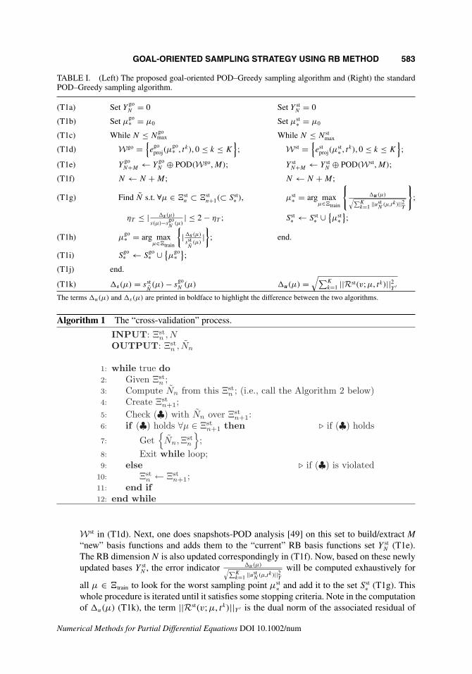
TABLE I. (Left) The proposed goal-oriented POD–Greedy sampling algorithm and (Right) the standardPOD–Greedy sampling algorithm.

(T1a) Set YgoN = 0 Set Y st

N = 0

(T1b) Set μgo∗ = μ0 Set μst∗ = μ0

(T1c) While N ≤ Ngomax While N ≤ N st

max

(T1d) Wgo ={e

goproj(μ

go∗ , tk), 0 ≤ k ≤ K

}; W st =

{est

proj(μst∗ , tk), 0 ≤ k ≤ K

};

(T1e) YgoN+M ← Y

goN ⊕ POD(Wgo, M); Y st

N+M ← Y stN ⊕ POD(W st, M);

(T1f) N ← N + M; N ← N + M;

(T1g) Find N s.t. ∀μ ∈ �stn ⊂ �st

n+1(⊂ Sst∗ ), μst∗ = arg maxμ∈�train

{�u(μ)√∑K

k=1 ||ustN

(μ,tk )||2Y

};

ηT ≤ | �s (μ)

s(μ)−sgoN

(μ)| ≤ 2 − ηT ; Sst∗ ← Sst∗ ∪ {

μst∗};

(T1h) μgo∗ = arg max

μ∈�train

{|�s (μ)

sstN

(μ)|}

; end.

(T1i) Sgo∗ ← S

go∗ ∪ {

μgo∗

};

(T1j) end.

(T1k) �s(μ) = sstN(μ) − s

goN (μ) �u(μ) =

√∑Kk=1 ||Rst(v; μ, tk)||2

Y ′The terms �u(μ) and �s(μ) are printed in boldface to highlight the difference between the two algorithms.

Algorithm 1 The “cross-validation” process.

W st in (T1d). Next, one does snapshots-POD analysis [49] on this set to build/extract M“new” basis functions and adds them to the “current” RB basis functions set Y st

N (T1e).The RB dimension N is also updated correspondingly in (T1f). Now, based on these newlyupdated bases Y st

N , the error indicator �u(μ)√∑Kk=1 ||ust

N(μ,tk )||2

Y

will be computed exhaustively for

all μ ∈ �train to look for the worst sampling point μst∗ and add it to the set Sst

∗ (T1g). Thiswhole procedure is iterated until it satisfies some stopping criteria. Note in the computationof �u(μ) (T1k), the term ||Rst(v; μ, t k)||Y ′ is the dual norm of the associated residual of


584 HOANG ET AL.

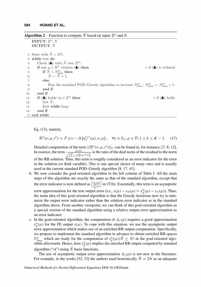
Algorithm 2 Function to compute N based on input �st and N.

Eq. (13), namely,

Rst(v; μ, t k) = F (v) − A(uk+1

N (μ), v; μ)

, ∀v ∈ YN , μ ∈ D, 1 ≤ k ≤ K − 1. (17)

Detailed computation of the term ||Rst(v; μ, t k)||Y ′ can be found in, for instance, [7, 8, 12].In essence, the term �u(μ)√∑K

k=1 ||ustN

(μ,tk )||2Y

is the ratio of the dual norm of the residual to the norm

of the RB solution. Thus, this term is roughly considered as an error indicator for the errorin the solution (or field variable). This is one special choice of many ones and is usuallyused in the current standard POD–Greedy algorithm [8, 17, 41].

b. We now consider the goal-oriented algorithm in the left column of Table I. All the mainsteps of this algorithm are exactly the same as that of the standard algorithm, except that

the error indicator is now defined as∣∣∣�s(μ)

sstN

(μ)

∣∣∣ in (T1h). Essentially, this term is an asymptotic

error approximation for the true output error (i.e., s(μ) − sN(μ) ≈ sstN(μ) − sN(μ)). Thus,

the main idea of this goal-oriented algorithm is that the Greedy iterations now try to min-imize the output error indicator rather than the solution error indicator as in the standardalgorithm above. From another viewpoint, we can think of this goal-oriented algorithm asa special version of the standard algorithm using a relative output error approximation asan error indicator.

c. In the goal-oriented algorithm, the computation of �s(μ) requires a good approximationsstN(μ) for the FE output s(μ). To cope with this situation, we use the asymptotic output

error approximation which makes use of an enriched RB output computation. Specifically,we propose to implement the standard algorithm in advance to obtain enriched RB spacesY st

Nmaxwhich are ready for the computation of sst

N(μ)(N ≥ N ) in the goal-oriented algo-

rithm afterwards. Hence, here sstN(μ) implies the enriched RB output computed by standard

algorithm (“st”) using N basis functions.The use of asymptotic output error approximation �s(μ) is not new in the literature.

For example, in the works [32, 33] the authors used heuristically N = 2N as an adequate



choice for the output error approximation. In this work, however, we propose a new algo-rithm called a “cross-validation” process to choose adaptively N for each particular N inthe offline stage of the goal-oriented algorithm. Note that these found pairs (N , N) willalso be used in the error approximation in the online stage later. The “cross-validation”process is presented in line (T1g) and is detailed in Algorithm 1; however, we postpone itsexplanation until point f) below.

d. The main idea of the “cross-validation” process is to find a sufficient N (for an N under

consideration) such that the effectivity∣∣∣ sst

N(μ)−s

goN

(μ)

s(μ)−sgoN

(μ)

∣∣∣ satisfies: ∀μ ∈ �try,

ηT ≤∣∣∣∣ s

stN(μ) − s

goN (μ)

s(μ) − sgoN (μ)

∣∣∣∣ ≤ 2 − ηT , (♣)

where ηT is a user-prescribed effectivity (say, 0.8 or 0.9), and �try is an arbitrary set ofparameters (sgo

N (μ) is a goal-oriented RB output using N basis functions). Because the FEoutput s(μ) appears in (♣), we think of using �try ⊂ Sst

∗ as all FE solutions/outputs areavailable for all μ ∈ Sst

∗ (recall that the standard algorithm was already implemented).Hence, we will use the notation �st(≡ �try) ⊂ Sst

∗ to reflect this idea.e. We first explain the Algorithm 2 in detail. Essentially, algorithm 2 is an iteration process

to find a proper N which satisfies (♣) for a given sample set �st and a given N. Theiteration procedure starts with N = 2N ; and N will be increased if (♣) is violated byany μ ∈ �st. The procedure will stop when (♣) holds true ∀μ ∈ �st. Within Algorithm2, if N exceeds N st

max the standard algorithm will be called and implemented to increaseN st

max accordingly. Note that the standard algorithm will continue to run from the previousN st

max; so in summary, it is deemed to run “once” but continuously in different stages whennecessary.

f. Let us now describe the “cross-validation” process in Algorithm 1. In fact, finding theproper size of �st is not a trivial task: fixing �st = Sst

∗ is not an efficient way, and wealso don’t want to use one more parameter to tune this setting (the only one parameter forthe GO algorithm is ηT ). We thus propose an adaptive strategy to choose |�st| as follows(Algorithm 1). Suppose that at the Greedy iteration N with a given set �st

n ⊂ Sst∗ , we can

find the corresponding N thanks to Algorithm 2 above. We will request further that thecurrently found N also needs to verify (♣) over �st

n+1, where |�stn+1| = |�st

n | + �nsample,and �nsample is a number of next sample points taken from the set Sst

∗ . Otherwise, �stn+1 is

assigned to �stn (i.e., �st

n is enriched now) and the procedure is repeated until the found N

satisfies (♣) over both sets �stn and �st

n+1 (⊂ Sst∗ ). By this way, we can start the sampling

procedure with fairly small |�stn | and let it “evolve” automatically without the necessity of

any control or adjustment. Following the same process, �stn and �st

n+1 will also be used tofind N at the next Greedy iteration N + 1; and they will be enriched appropriately whennecessary.

For example, the standard algorithm is implemented first and once for quite large N stmax,

say, N stmax = 200 and hence |Sst

∗ | = 200 (using M = 1). Then for an arbitrary quantity ofinterest, the goal-oriented algorithm will be implemented accordingly. Consider the “cross-validation” process at the first Greedy iterationN go = 1, we can choose�st

1 ⊂ �st2 ⊂ Sst

∗ suchthat |�st

1 | = 10 and |�st2 | = 20 first sample points of Sst

∗ , respectively (hence, �nsample = 10).Based on this �st

1 set, Algorithm 2 is invoked to find the corresponding N1. Next, (♣) ischecked with N1 over �st

2 : if it holds true ∀μ ∈ �st2 , then (N go = 1, N1) will be the necessar-

ily found pair; the algorithm will quit the “cross-validation” process and continue with step


586 HOANG ET AL.

(T1h). Otherwise, the algorithm will enrich �st1 and �st

2 such that |�st1 | = 20 and |�st

2 | = 30first sample points from Sst

∗ , and repeat the computational procedure until the right pair(N go = 1, N) is found. �st

1 and �st2 are also used to check (♣) at the next Greedy iteration

in a completely similar manner.g. Finally, we close this subsection with one remark on the possible value range of ηT . In fact,

we cannot choose ηT to be too high, that is, too close to 1. The reason is that the convergenceof the GO algorithm depends on the convergence of the standard one; and generally thestandard algorithm will stall/flat with some N ≥ N st

max (i.e., its error indicator and RB trueerror cannot decrease further as it reaches machine accuracy ≈ 10−8). If ηT is too close to 1,say 0.95, the cross-validation process will break down (infinite loop in Algorithm 1) sinceit cannot find the suitable N to satisfy (♣) over �st

n and �stn+1; and there is no way to handle

this situation. Therefore, it is practical to choose a modest ηT , and in fact we can do thateasily based on the convergence history of the standard algorithm which is implemented inadvance. Indeed, through two numerical experiments in Section IV later, ηT = 0.8 is themaximum possible choice and it gives the best performance among all GO ηT algorithms.On the contrary, low ηT (i.e., close to 0) poses no difficulty for the cross-validation processsince its corresponding N generally will be smaller than that of higher ηT , and hence lowηT is “safer” than high ηT regarding N .

C. Error Estimations

True Errors. We use the true errors to validate the performance of the standard and goal-orientedalgorithms in the online computation stage. The relative true errors by the two algorithms for thesolutions are defined as

estu (μ) =

√∑K

k=1 ||uk(μ) − ust,kN (μ)||2Y∑K

k=1 ||uk(μ)||2Y, ego

u (μ) =√∑K

k=1 ||uk(μ) − ugo,kN (μ)||2Y∑K

k=1 ||uk(μ)||2Y; (18)

and for the outputs

ests (μ) =

∣∣∣∣ s(μ) − sstN(μ)

s(μ)

∣∣∣∣ ≈∣∣∣∣∑K−1

k=0�t

2

(�(uk(μ) − u

st,kN (μ)

) + �(uk+1(μ) − u

st,k+1N (μ)

))∑K−1

k=0�t

2

(�(uk(μ)) + �(uk+1(μ))

) ∣∣∣∣,(19a)

egos (μ) =

∣∣∣∣ s(μ) − sgoN (μ)

s(μ)

∣∣∣∣ ≈∣∣∣∣∑K−1

k=0�t

2

(�(uk(μ) − u

go,kN (μ)

)+ �

(uk+1(μ) − u

go,k+1N (μ)

))∑K−1

k=0�t

2

(�(uk(μ)) + �(uk+1(μ))

) ∣∣∣∣,(19b)

respectively.In the above expressions, uk(μ), ust,k

N (μ) and ugo,kN (μ) are the FE, standard RB and goal-oriented

RB solutions; s(μ), sstN(μ) and s

goN (μ) are the FE, standard RB, and goal-oriented RB outputs,

respectively.

Output Error Approximation. The true errors are good for validation purposes but are not ofpractical uses in the online stage, where one requires fast and countless online calculations. In thiswork, we propose to use �s(μ) as an error estimation for the output in the online computationstage (in short, �s(μ) is an error estimation in both offline and online stages). Of course this error



approximation is not a rigorous upper error bound such as the a posteriori error bounds [7, 15, 17];however, there are several good reasons for using it in practice. First, the time-marching errorbounds for the wave equation so far were shown to be ineffective and pessimistic due to theinstability of the wave equation: exponential growing with respect to time [19, 52, 53]. (We alsonote that the space-time error bounds, although very promising, are still not yet derived in theliterature.) Second, this error approximation converges asymptotically to the true error (thanksto N chosen effectively by the proposed “cross-validation” process), and thus can approximaterelatively the accuracy of the RB outputs for various choices of μ. Third—most important, itscomputational cost is cheap: only O(N 3)+O(N 3) as described in the next section (N , N � N ).The output error approximation �s(μ) in (T1k) and its associated effectivity are defined asfollows

�gos (μ) = sst

N(μ) − s

goN (μ), ηgo

s (μ) =∣∣∣∣ �go

s (μ)

s(μ) − sgoN (μ)

∣∣∣∣. (20)

Note that to compare the performance of output error approximation of the standard versus thegoal-oriented algorithms, here we also define the output error approximation and its associatedeffectivity for the standard algorithm as

�sts (μ) = sst

N(μ) − sst

N(μ), ηsts (μ) =

∣∣∣∣ �sts (μ)

s(μ) − sstN(μ)

∣∣∣∣, (21)

where the superscript “st” implies the standard algorithm. The superscript “go” is thus added in(20) to imply the goal-oriented algorithm, respectively.

D. Offline-Online Computational Procedure

In this section, we develop offline-online computational procedures to fully exploit the dimensionreduction of the problem [8, 12, 15]. We note that both algorithms (standard and goal-oriented)have the same offline-online computational procedures, they are only different in the ways tobuild the sets S∗ and YN via Greedy iterations. We first express uk

N(μ) as:

ukN(μ) =

N∑n=1

ukNn(μ)ζn, ∀ζn ∈ YN . (22)

We then choose a test function v = ζn, 1 ≤ n ≤ N for the RB Eq. (13). It then follows thatuk

N(μ) = [ukN1(μ)uk

N2(μ) · · · ukNN(μ)]T ∈ R

N satisfies

(1

�t2MN(μ) + 1

2�tCN(μ) + 1

4AN(μ)

)uk+1

N (μ)

=(

− 1

�t2MN(μ) + 1

2�tCN(μ) − 1

4AN(μ)

)uk−1

N (μ)

+(

2

�t2MN(μ) − 1

2AN(μ)

)uk

N(μ) + geq(tk)FN(μ), 1 ≤ k ≤ K − 1. (23)


588 HOANG ET AL.

The initial condition is treated similar to the treatment in (9) and (13). Here,CN(μ), AN(μ), MN(μ) ∈ R

N×N are symmetric positive definite matrices5 with entries CNi,j (μ) =c(ζi , ζj ; μ), ANi,j (μ) = a(ζi , ζj ; μ), MNi,j (μ) = m(ζi , ζj ; μ), 1 ≤ i, j ≤ N and FN ∈ R

N is theRB load vector with entries FNi = f (ζi), 1 ≤ i ≤ N , respectively.

The RB output is then computed from

sN(μ) =K−1∑k=0

�t

2LT

N

(uk

N(μ) + uk+1N (μ)

). (24)

Invoking the affine parameter dependence (8), we obtain

MNi,j (μ) = m(ζi , ζj ; μ) =Qm∑q=1

�qm(μ)mq(ζi , ζj ), (25a)

CNi,j (μ) = c(ζi , ζj ; μ) =Qc∑q=1

�qc (μ)cq(ζi , ζj ), (25b)

ANi,j (μ) = a(ζi , ζj ; μ) =Qa∑q=1

�qa(μ)aq(ζi , ζj ), (25c)

FNi(μ) = f (ζi ; μ) =Qf∑q=1

�q

f (μ)f q(ζi), (25d)

which can be written as

MNi,j (μ) =Qm∑q=1

�qm(μ)Mq

Ni,j , CNi,j (μ) =Qc∑q=1

�qc (μ)Cq

Ni,j ,

ANi,j (μ) =Qa∑q=1

�qa(μ)Aq

Ni,j , FNi(μ) =Qf∑q=1

�q

f (μ)Fq

Ni , (26)

where the parameter independent quantities Mq

N , Cq

N , Aq

N ∈ RN×N , and Fq

N ∈ RN are given by

Mq

Ni,j = mq(ζi , ζj ), 1 ≤ i, j ≤ Nmax, 1 ≤ q ≤ Qm, (27a)

Cq

Ni,j = cq(ζi , ζj ), 1 ≤ i, j ≤ Nmax, 1 ≤ q ≤ Qc, (27b)

Aq

Ni,j = aq(ζi , ζj ), 1 ≤ i, j ≤ Nmax, 1 ≤ q ≤ Qa , (27c)

Fq

Ni = f q(ζi), 1 ≤ i ≤ Nmax, 1 ≤ q ≤ Qf , (27d)

respectively.The offline-online computational procedure is now described as follows. In the offline stage—

performed only once, we first implement the standard POD–Greedy algorithm [8]: we solve to

5 The proof of this property can be found in, for instance, Proposition 5.1, page 136 of [54]. Thanks to this property, thestability of our proposed RB scheme will be guaranteed as a consequence.



find Y stN = {ζ st

n , 1 ≤ n ≤ Nmax}; then compute and store the μ-independent quantities in (27) forthe estimation of the RB solution and output6. Once these RB solution and output are available, wecan now implement the goal-oriented POD–Greedy algorithm. We consider each goal-orientedPOD–Greedy iteration (Table I) in more details. We first need to solve (9) for the “true” FEsolutions; then compute the projection error in step (T1d) and solve the POD/eigenvalue problemin step (T1e). In addition, we have to compute O(N 2Q)N -inner products in (27) (we denoteQ = Qm + Qc + Qa). By approximating s(μ) via the enriched approximation sst

N(μ) in (T1k)

through the standard algorithm, we can now do an exhaustive yet cheap search over �train to lookfor the optimal μ in each Greedy iteration. In summary, the offline stage of the goal-orientedalgorithm also includes the offline stage of the standard algorithm, and therefore, it is moreexpensive than that of the standard algorithm. (We again emphasize that the standard algorithmis implemented only once, and then the goal-oriented algorithm can be implemented many timescorresponding with various output functionals, respectively.).

The online stage of the goal-oriented algorithm is very similar to that of the standard algorithm[8]. In the online stage—performed many times, for each new parameter μ—we first assemblethe RB matrices in (25), this requires O(N 2Q) operations. We then solve the RB governing Eq.(23), the operation counts are O(N 3 + KN 2) as the RB matrices are generally full. Finally, weevaluate the displacement output sN(μ) from (24) at the cost of O(KN). For the error approxi-mation (i.e., �s(μ) = sst

N(μ) − s

goN (μ)), there is nothing more than computing one more output

sstN(μ) and then performing the associated subtraction; the cost is O(N 3). Therefore, as required

in the real-time context, the online complexity to compute the output and its associated errorapproximation are O(N 3) + O(N 3)—independent of N ; and since N , N � N we can expectsignificant computational saving in the online stage relative to the classical FE approach.

IV. NUMERICAL EXAMPLES

In this section, we will verify both POD–Greedy algorithms by investigating a simple 2D linearelastodynamic problem and a 3D dental implant model problem in the time domain. The detailsare described in the following.

A. A 2D Linear Elastodynamic Problem

Finite Element Model and Approximation. We consider a 2D plane strain model problemas in Fig. 1(a). It is assumed that the model problem is scaled (or nondimensionalized) from a realproblem in practice and hence all the terms are dimensionless. The details of the nondimensional-ization is briefly discussed in Appendix A. The length and height of the model are L = 4 and H = 1,respectively. The model is composed of 2 subdomains �1 and �2 with two different materials:Young’s moduli E1 = 1 and E2 ∈ [0.1, 10] and Poisson ratios ν1 = ν2 = 0.3, respectively.We assume Rayleigh damping for the model where the mass-proportional damping coefficientsα1 = α2 = 0, and the stiffness-proportional damping coefficients β1 = β2 ≡ β ∈ [0.05, 0.5] suchthat Ci = βiAi , 1 ≤ i ≤ 2, where Ci and Ai are the FEM damping and stiffness matrices of eachsubdomain, respectively. Isotropic and homogenous material behavior is assumed for the model.We also note that the material mass densities will vanish from the weak form of the PDE due to

6 There are still several terms related to the computation of the dual norm of the residual ||Rst(v; μ, tk)||Y ′ , we do notshow them here for simplicity. Detailed implementation of the standard POD–Greedy algorithm can be referred to, forinstance, [8, 15, 17].


590 HOANG ET AL.

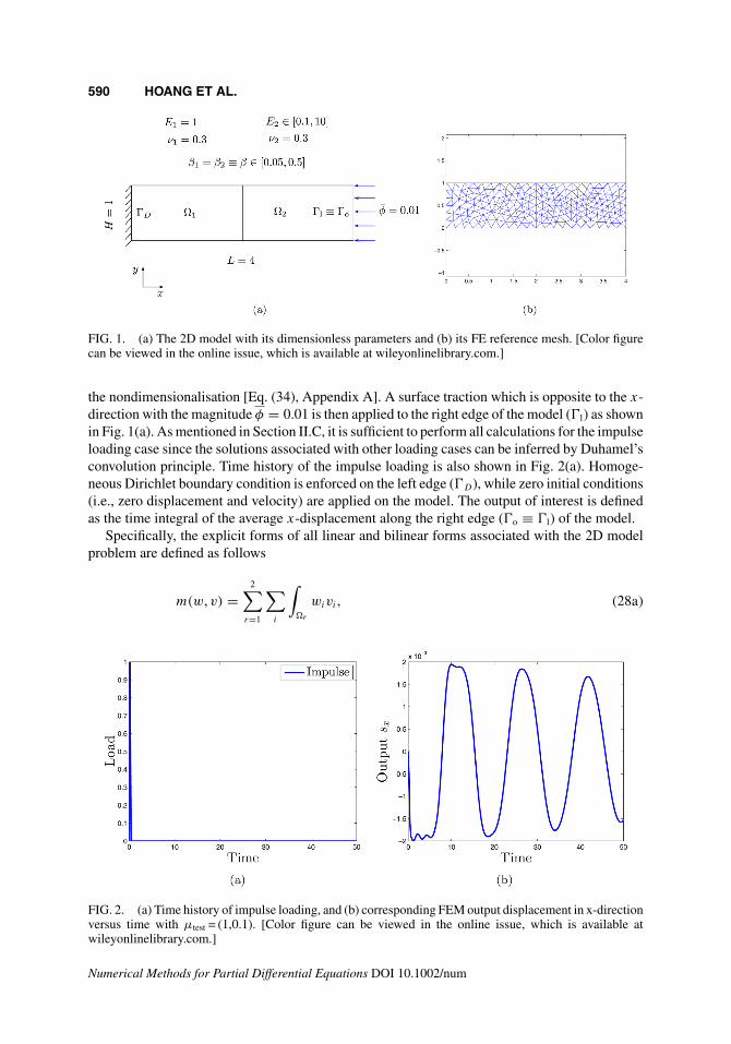
FIG. 1. (a) The 2D model with its dimensionless parameters and (b) its FE reference mesh. [Color figurecan be viewed in the online issue, which is available at wileyonlinelibrary.com.]

the nondimensionalisation [Eq. (34), Appendix A]. A surface traction which is opposite to the x-direction with the magnitude φ = 0.01 is then applied to the right edge of the model (�l) as shownin Fig. 1(a). As mentioned in Section II.C, it is sufficient to perform all calculations for the impulseloading case since the solutions associated with other loading cases can be inferred by Duhamel’sconvolution principle. Time history of the impulse loading is also shown in Fig. 2(a). Homoge-neous Dirichlet boundary condition is enforced on the left edge (�D), while zero initial conditions(i.e., zero displacement and velocity) are applied on the model. The output of interest is definedas the time integral of the average x-displacement along the right edge (�o ≡ �l) of the model.

Specifically, the explicit forms of all linear and bilinear forms associated with the 2D modelproblem are defined as follows

m(w, v) =2∑

r=1

∑i

∫�r

wivi , (28a)

FIG. 2. (a) Time history of impulse loading, and (b) corresponding FEM output displacement in x-directionversus time with μtest = (1,0.1). [Color figure can be viewed in the online issue, which is available atwileyonlinelibrary.com.]



a(w, v; μ) =∑i,j ,k,l

∫�1

∂vi

∂xj

C1ijkl

∂wk

∂xl

+ μ1

∑i,j ,k,l

∫�2

∂vi

∂xj

C2ijkl

∂wk

∂xl

, (28b)

c(w, v; μ) = μ2

∑i,j ,k,l

∫�1

∂vi

∂xj

C1ijkl

∂wk

∂xl

+ μ2μ1

∑i,j ,k,l

∫�2

∂vi

∂xj

C2ijkl

∂wk

∂xl

, (28c)

f (v) =∑

i

∫�l

viφi , (28d)

�(v) = 1

|�o|∫

�o

v1, (28e)

for all w, v ∈ Y , μ ∈ D. Here, the parameter μ = (μ1, μ2) ≡ (E2, β), where E2 is the Young’smodulus of the domain �2 and β is the stiffness-proportional damping coefficient of both domains�1, �2.Cr

ijkl is the constitutive elasticity tensor for isotropic materials and it is expressed in terms ofthe Young’s modulus E and Poisson’s ratio ν of each region �r , 1 ≤ r ≤ 2, respectively. It is obvi-ous from (8) and (28) that the smooth functions �1

a(μ) = 1, �2a(μ) = μ1; �1

c(μ) = μ2, �2c(μ) =

μ1μ2 depend on μ — but the bilinear forms a1(w, v) = c1(w, v) = ∑i,j ,k,l

∫�1

∂vi

∂xjC1

ijkl

∂wk

∂xl, and

a2(w, v) = c2(w, v) = ∑i,j ,k,l

∫�2

∂vi

∂xjC2

ijkl

∂wk

∂xldo not depend on μ.

The FE mesh consist of 215 nodes and 376 linear triangular elements as shown in Fig. 1(b).The FE space to approximate the 2D elastodynamic problem is of dimension N = 416. For timeintegration, T = 50, �t = 0.2, K = T

�t= 250. The parameter μ = (E2, β) ∈ D, where the

parameter domain D ≡ [0.1, 10] × [0.05, 0.5] ⊂ RP=2. The || · ||Y used in this work is defined

as ||w||2Y = a(w, w; μ) + m(w, w; μ), where μ = (1, 0.1); Qa = 2, Qc = 2. The entire work isperformed using the software MATLAB R2012b. We finally show in Fig. 2(b) the “unit” FEMoutput displacement (i.e., under the unit impulse load) in the x-direction versus time at μtest, whereμtest = μ = (1, 0.1).

Numerical Results

The Impulse Loading Case. For this 2D model problem, we aim to investigate the behaviorof the goal-oriented algorithms with various choices of ηT under the impulse loading regime.To start, a training sample set �train is created by an equidistant distribution over D withntrain(= 30 × 30) = 900 samples. Note that we use M = 1 and N go

max = 60 (as in Table I)to terminate the iteration procedures. In the remaining sections, beside the standard and goal-oriented algorithms (ηT ), we also show the results of the goal-oriented algorithm (N = 2N ) forcomparison purpose.

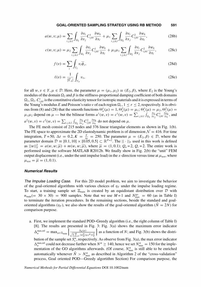
a. First, we implement the standard POD–Greedy algorithm (i.e., the right column of Table I)[8]. The results are presented in Fig. 3: Fig. 3(a) shows the maximum error indicator

�max,relu = maxμ∈�train

{�u(μ)√∑K

k=1 ||ustN

(μ,tk )||2Y

}as a function of N ; and Fig. 3(b) shows the distri-

bution of the sample set Sst∗ , respectively. As observe from Fig. 3(a), the max error indicator

�max,relu could not decrease further when N st ≥ 140, hence we set N st

max = 150 for the imple-mentation of the GO algorithms afterwards. (Of course, N st

max is still able to be enrichedautomatically whenever N > N st

max as described in Algorithm 2 of the “cross-validation”process, Goal oriented POD—Greedy algortithm Section) For comparison purpose, the


592 HOANG ET AL.

FIG. 3. (a) Maximum of error indicator �max,relu over �train as a function of N, and (b) distribution of

sampling points by the standard POD–Greedy algorithm (N stmax = 150). Different markers were used for

the first N stmax = 60 basis functions. [Color figure can be viewed in the online issue, which is available at

wileyonlinelibrary.com.]

results associated with the first N stmax = 60 basis functions were plotted using different

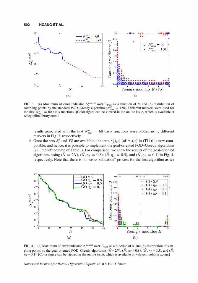
markers in Fig. 3, respectively.b. Once the sets Sst

∗ and Y stN are available, the term sst

N(μ) (of �s(μ) in (T1k)) is now com-

putable; and hence, it is possible to implement the goal-oriented POD–Greedy algorithms(i.e., the left column of Table I). For comparison, we show the results of the goal-orientedalgorithms using (N = 2N ), (N , ηT = 0.8), (N , ηT = 0.5), and (N , ηT = 0.1) in Fig. 4,respectively. Note that there is no “cross-validation” process for the first algorithm as we

FIG. 4. (a) Maximum of error indicator �max,rels over �train as a function of N and (b) distribution of sam-

pling points by the goal-oriented POD–Greedy algorithms (N= 2N), (N , ηT = 0.8), (N , ηT = 0.5), and (N ,ηT = 0.1). [Color figure can be viewed in the online issue, which is available at wileyonlinelibrary.com.]



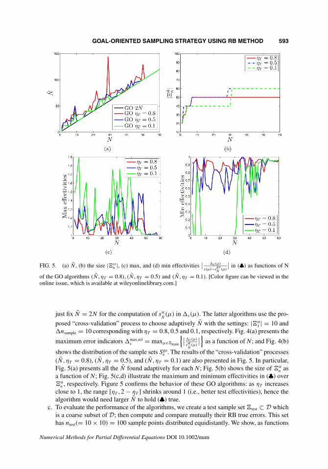
FIG. 5. (a) N , (b) the size |�stn |, (c) max, and (d) min effectivities

∣∣ �s(μ)

s(μ)−sgoN

(μ)

∣∣ in (♣) as functions of N

of the GO algorithms (N , ηT = 0.8), (N , ηT = 0.5) and (N , ηT = 0.1). [Color figure can be viewed in theonline issue, which is available at wileyonlinelibrary.com.]

just fix N = 2N for the computation of sstN(μ) in �s(μ). The latter algorithms use the pro-

posed “cross-validation” process to choose adaptively N with the settings: |�st1 | = 10 and

�nsample = 10 corresponding with ηT = 0.8, 0.5 and 0.1, respectively. Fig. 4(a) presents the

maximum error indicators �max,rels = maxμ∈�train

{∣∣�s(μ)

sstN

(μ)

∣∣} as a function of N ; and Fig. 4(b)

shows the distribution of the sample sets Sgo∗ . The results of the “cross-validation” processes

(N , ηT = 0.8), (N , ηT = 0.5), and (N , ηT = 0.1) are also presented in Fig. 5. In particular,Fig. 5(a) presents all the N found adaptively for each N ; Fig. 5(b) shows the size of �st

n asa function of N ; Fig. 5(c,d) illustrate the maximum and minimum effectivities in (♣) over�st

n , respectively. Figure 5 confirms the behavior of these GO algorithms: as ηT increasesclose to 1, the range [ηT , 2 − ηT ] shrinks around 1 (i.e., better test effectivities), hence thealgorithm would need larger N to hold (♣) true.

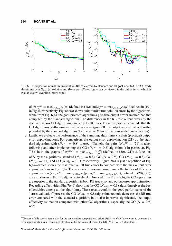
c. To evaluate the performance of the algorithms, we create a test sample set �test ⊂ D whichis a coarse subset of D; then compute and compare mutually their RB true errors. This sethas ntest(= 10 × 10) = 100 sample points distributed equidistantly. We show, as functions


594 HOANG ET AL.

FIG. 6. Comparison of maximum (relative) RB true errors by standard and all goal-oriented POD–Greedyalgorithms over �test: (a) solution and (b) output. [Color figure can be viewed in the online issue, which isavailable at wileyonlinelibrary.com.]

of N : emaxu = maxμ∈�testeu(μ) (defined in (18)) and emax

s = maxμ∈�testes(μ) (defined in (19))in Fig. 6, respectively. Figure 6(a) shows quite similar true solution errors by the algorithms;while from Fig. 6(b), the goal-oriented algorithms give true output errors smaller than thatcomputed by the standard algorithm. The differences in the RB true output errors by thestandard versus GO algorithms can be up to 10 times. Therefore, we can conclude that theGO algorithms (with cross-validation processes) give RB true output errors smaller than thatprovided by the standard algorithm (for the same N basis functions under consideration).

d. Lastly, we evaluate the performance of the sampling algorithms via their (practical) outputerror approximations. For comparison, the output error approximation (21) by the stan-dard algorithm with (N , ηT = 0.8) is used. (Namely, the pairs (N , N) in (21) is takenfollowing and after implementing the GO (N , ηT = 0.8) algorithm.7) In particular, Fig.7(b) shows the graphs of �max,rel

s = maxμ∈�test |�s(μ)

s(μ)| (defined in (20), (21)) as functions

of N by the algorithms: standard (N , ηT = 0.8), GO (N = 2N ), GO (N , ηT = 0.8), GO(N , ηT = 0.5), and GO (N , ηT = 0.1), respectively. Figure 7(a) is just a repetition of Fig.6(b)—which shows the max relative RB true errors to compare with the max output errorapproximations in Fig. 7(b). The associated maximum/minimum effectivities of this errorapproximation (i.e., ηmax

s = maxμ∈�testηs(μ), ηmins = minμ∈�testηs(μ), defined in (20), (21))

are also shown in Fig. 7(c,d), respectively. As observed from Fig. 7(a,b), the GO algorithmsare superior to the standard algorithm in both RB true error and output error approximation.Regarding effectivities, Fig. 7(c,d) show that the GO (N , ηT = 0.8) algorithm gives the besteffectivities among all the algorithms. These results confirm the good performance of the“cross-validation” process: the GO (N , ηT = 0.8) algorithm not only decreases the RB trueerror compared with the standard algorithm, but it also improves significantly the outputeffectivity estimation compared with other GO algorithms (especially the GO (N = 2N )one).

7 The aim of this special test is that for the same online computational effort O(N3) + O(N3), we want to compare theerror approximations and associated effectivities by the standard versus the GO (N , ηT = 0.8) algorithms.



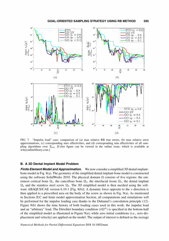
FIG. 7. “Impulse load” case: comparison of (a) max relative RB true errors, (b) max relative errorapproximations, (c) corresponding max effectivities, and (d) corresponding min effectivities of all sam-pling algorithms over �test. [Color figure can be viewed in the online issue, which is available atwileyonlinelibrary.com.]

B. A 3D Dental Implant Model Problem

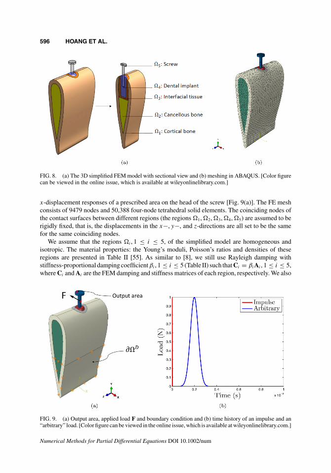
Finite Element Model and Approximation. We now consider a simplified 3D dental implant-bone model in Fig. 8(a). The geometry of the simplified dental implant-bone model is constructedusing the software SolidWorks 2010. The physical domain � consists of five regions: the out-ermost cortical bone �1, the cancellous bone �2, the interfacial tissue �3, the dental implant�4 and the stainless steel screw �5. The 3D simplified model is then meshed using the soft-ware ABAQUS/CAE version 6.10-1 [Fig. 8(b)]. A dynamic force opposite to the x-direction isthen applied to a prescribed area on the body of the screw as shown in Fig. 9(a). As mentionedin Sections II.C and finite model approximation Section, all computations and simulations willbe performed for the impulse loading case thanks to the Duhamel’s convolution principle (12).Figure 9(b) shows the time history of both loading cases used in this work: the impulse loadand an “arbitrary” load. The Dirichlet boundary condition (∂�D) is specified in the bottom-halfof the simplified model as illustrated in Figure 9(a); while zero initial conditions (i.e., zero dis-placement and velocity) are applied on the model. The output of interest is defined as the average


596 HOANG ET AL.

FIG. 8. (a) The 3D simplified FEM model with sectional view and (b) meshing in ABAQUS. [Color figurecan be viewed in the online issue, which is available at wileyonlinelibrary.com.]

x-displacement responses of a prescribed area on the head of the screw [Fig. 9(a)]. The FE meshconsists of 9479 nodes and 50,388 four-node tetrahedral solid elements. The coinciding nodes ofthe contact surfaces between different regions (the regions �1, �2, �3, �4, �5) are assumed to berigidly fixed, that is, the displacements in the x−, y−, and z-directions are all set to be the samefor the same coinciding nodes.

We assume that the regions �i , 1 ≤ i ≤ 5, of the simplified model are homogeneous andisotropic. The material properties: the Young’s moduli, Poisson’s ratios and densities of theseregions are presented in Table II [55]. As similar to [8], we still use Rayleigh damping withstiffness-proportional damping coefficientβi , 1 ≤ i ≤ 5 (Table II) such that Ci = βiAi , 1 ≤ i ≤ 5,where Ci and Ai are the FEM damping and stiffness matrices of each region, respectively. We also

FIG. 9. (a) Output area, applied load F and boundary condition and (b) time history of an impulse and an“arbitrary” load. [Color figure can be viewed in the online issue, which is available at wileyonlinelibrary.com.]



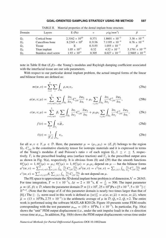
TABLE II. Material properties of the dental implant-bone structure.

Domain Layers E (Pa) ν ρ(g/mm3) β

�1 Cortical bone 2.3162 × 1010 0.371 1.8601 × 10−3 3.38 × 10−6

�2 Cancellous bone 8.2345 × 108 0.3136 7.1195 × 10−4 6.76 × 10−6

�3 Tissue E 0.3155 1.055 × 10−3 β

�4 Titan implant 1.05 × 1011 0.32 4.52 × 10−3 5.1791 × 10−10

�5 Stainless steel screw 1.93 × 1011 0.305 8.027 × 10−3 2.5685 × 10−8

note in Table II that (E,β)—the Young’s modulus and Rayleigh damping coefficient associatedwith the interfacial tissue are our sole parameters.

With respect to our particular dental implant problem, the actual integral forms of the linearand bilinear forms are defined as:

m(w, v) =5∑

r=1

∑i

∫�r

ρrwivi , (29a)

a(w, v; μ) =5∑

r=1,r �=3

∑i,j ,k,l

∫�r

∂vi

∂xj

Crijkl

∂wk

∂xl

+ μ1

∑i,j ,k,l

∫�3

∂vi

∂xj

C3ijkl

∂wk

∂xl

, (29b)

c(w, v; μ) =5∑

r=1,r �=3

βr

∑i,j ,k,l

∫�r

∂vi

∂xj

Crijkl

∂wk

∂xl

+ μ2μ1

∑i,j ,k,l

∫�3

∂vi

∂xj

C3ijkl

∂wk

∂xl

, (29c)

f (v) =∑

i

∫�l

viφi , (29d)

�(v) = 1

|�o|∫

�o

v1, (29e)

for all w, v ∈ Y , μ ∈ D. Here, the parameter μ = (μ1, μ2) ≡ (E, β) belongs to the region�3. Cr

ijkl is the constitutive elasticity tensor for isotropic materials and it is expressed in termsof the Young’s modulus E and Poisson’s ratio ν of each region �r , 1 ≤ r ≤ 5, respec-tively. �l is the prescribed loading area (surface traction) and �o is the prescribed output areaas shown in Fig. 9(a), respectively. It is obvious from (8) and (29) that the smooth functions�1

a(μ) = 1, �2a(μ) = μ1; �1

c(μ) = 1, �2c(μ) = μ1μ2 depend on μ — but the bilinear forms

a1(w, v) = ∑5r=1,r �=3

∑i,j ,k,l

∫�r

∂vi

∂xjCr

ijkl

∂wk

∂xl, a2(w, v) = c2(w, v) = ∑

i,j ,k,l

∫�3

∂vi

∂xjC3

ijkl

∂wk

∂xland

c1(w, v) = ∑5r=1,r �=3 βr

∑i,j ,k,l

∫�r

∂vi

∂xjCr

ijkl

∂wk

∂xldo not depend on μ.

The FE space to approximate the 3D dental implant-bone problem is of dimension N = 26343.For time integration, T = 1 × 10−3s, �t = 2 × 10−6s, K = T

�t= 500. The input parameter

μ ≡ (E, β) ∈ D, where the parameter domain D ≡ [1×106, 25×106]Pa×[5×10−6, 5×10−5] ⊂R

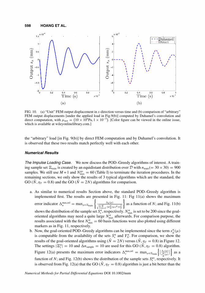
P=2. (Note that the range of E of this parameter domain is nearly two times larger than that of[8].) The || · ||Y norm used in this work is defined as ||w||2Y = a(w, w; μ) + m(w, w; μ), whereμ = (13 × 106Pa, 2.75 × 10−5) is the arithmetic average of μ in D; Qa = 2, Qc = 2. The entirework is performed using the software MATLAB R2012b. Figure 10 presents some FEM resultscorresponding with the test parameter μtest = (10 × 106Pa, 1 × 10−5). In particular, Fig. 10(a)shows the “unit” FEM output displacement (i.e., under the unit impulse load) in the xx-directionversus time at μtest. In addition, Fig. 10(b) shows the FEM output displacements versus time under


598 HOANG ET AL.

FIG. 10. (a) “Unit” FEM output displacement in x-direction versus time and (b) comparison of “arbitrary”FEM output displacements [under the applied load in Fig.9(b)] computed by Duhamel’s convolution anddirect computation, with μtest = (

10 × 106Pa, 1 × 10−5). [Color figure can be viewed in the online issue,

which is available at wileyonlinelibrary.com.]

the “arbitrary” load [in Fig. 9(b)] by direct FEM computation and by Duhamel’s convolution. Itis observed that these two results match perfectly well with each other.

Numerical Results

The Impulse Loading Case. We now discuss the POD–Greedy algorithms of interest. A train-ing sample set �train is created by an equidistant distribution over D with ntrain(= 30 × 30) = 900samples. We still use M = 1 and N go

max = 60 (Table I) to terminate the iteration procedures. In theremaining sections, we only show the results of 3 typical algorithms which are the standard, theGO (N , ηT = 0.8) and the GO (N = 2N ) algorithms for comparison.

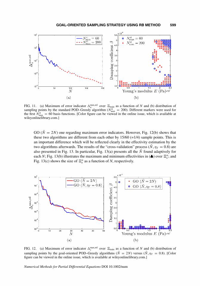
a. As similar to numerical results Section above, the standard POD–Greedy algorithm isimplemented first. The results are presented in Fig. 11: Fig 11(a) shows the maximum

error indicator �max,relu = maxμ∈�train

{�u(μ)√∑K

k=1 ||ustN

(μ,tk )||2Y

}as a function of N ; and Fig. 11(b)

shows the distribution of the sample set Sst∗ , respectively. N st

max is set to be 200 since the goal-oriented algorithms may need a quite large N st

max afterwards. For comparison purpose, theresults associated with the first N st

max = 60 basis functions were also plotted using differentmarkers as in Fig. 11, respectively.

b. Now, the goal-oriented POD–Greedy algorithms can be implemented since the term sstN(μ)

is computable from the availability of the sets Sst∗ and Y st

N . For comparison, we show theresults of the goal-oriented algorithms using (N = 2N ) versus (N , ηT = 0.8) in Figure 12.The settings |�st

1 | = 10 and �nsample = 10 are used for this GO (N , ηT = 0.8) algorithm.

Figure 12(a) presents the maximum error indicators �max,rels = maxμ∈�train

{∣∣�s(μ)

sstN

(μ)

∣∣} as a

function of N ; and Fig. 12(b) shows the distribution of the sample sets Sgo∗ , respectively. It

is observed from Fig. 12(a) that the GO (N , ηT = 0.8) algorithm is just a bit better than the



FIG. 11. (a) Maximum of error indicator �max,relu over �train as a function of N and (b) distribution of

sampling points by the standard POD–Greedy algorithm (N stmax = 200). Different markers were used for

the first N stmax = 60 basis functions. [Color figure can be viewed in the online issue, which is available at

wileyonlinelibrary.com.]

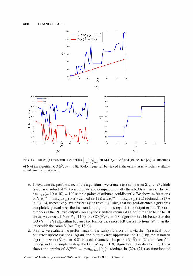
GO (N = 2N ) one regarding maximum error indicators. However, Fig. 12(b) shows thatthese two algorithms are different from each other by 15/60 (=1/4) sample points. This isan important difference which will be reflected clearly in the effectivity estimation by thetwo algorithms afterwards. The results of the “cross-validation” process (N , ηT = 0.8) arealso presented in Fig. 13. In particular, Fig. 13(a) presents all the N found adaptively foreach N ; Fig. 13(b) illustrates the maximum and minimum effectivities in (♣) over �st

n ; andFig. 13(c) shows the size of �st

n as a function of N, respectively.

FIG. 12. (a) Maximum of error indicator �max,rels over �train as a function of N and (b) distribution of

sampling points by the goal-oriented POD–Greedy algorithms (N = 2N ) versus (N , ηT = 0.8). [Colorfigure can be viewed in the online issue, which is available at wileyonlinelibrary.com.]


600 HOANG ET AL.

FIG. 13. (a) N , (b) max/min effectivities∣∣∣ �s(μ)

s(μ)−sgoN

(μ)

∣∣∣ in (♣), ∀μ ∈ �stn ,and (c) the size |�st

n | as functions

of N of the algorithm GO (N , ηT = 0.8). [Color figure can be viewed in the online issue, which is availableat wileyonlinelibrary.com.]

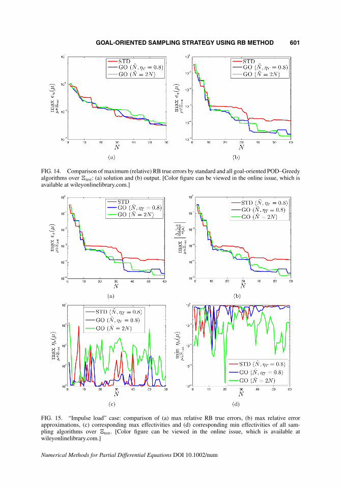
c. To evaluate the performance of the algorithms, we create a test sample set �test ⊂ D whichis a coarse subset of D; then compute and compare mutually their RB true errors. This sethas ntest(= 10 × 10) = 100 sample points distributed equidistantly. We show, as functionsof N : emax

u = maxμ∈�testeu(μ) (defined in (18)) and emaxs = maxμ∈�testes(μ) (defined in (19))

in Fig. 14, respectively. We observe again from Fig. 14(b) that the goal-oriented algorithmscompletely prevail over the the standard algorithm as regards true output errors. The dif-ferences in the RB true output errors by the standard versus GO algorithms can be up to 10times. As expected from Fig. 14(b), the GO (N , ηT = 0.8) algorithm is a bit better than theGO (N = 2N ) algorithm because the former uses more RB basis functions (N ) than thelatter with the same N [see Fig. 13(a)].

d. Finally, we evaluate the performance of the sampling algorithms via their (practical) out-put error approximations. Again, the output error approximation (21) by the standardalgorithm with (N , ηT = 0.8) is used. (Namely, the pairs (N , N) in (21) is taken fol-lowing and after implementing the GO (N , ηT = 0.8) algorithm.) Specifically, Fig. 15(b)shows the graphs of �max,rel

s = maxμ∈�test |�s(μ)

s(μ)| (defined in (20), (21)) as functions of



FIG. 14. Comparison of maximum (relative) RB true errors by standard and all goal-oriented POD–Greedyalgorithms over �test: (a) solution and (b) output. [Color figure can be viewed in the online issue, which isavailable at wileyonlinelibrary.com.]

FIG. 15. “Impulse load” case: comparison of (a) max relative RB true errors, (b) max relative errorapproximations, (c) corresponding max effectivities and (d) corresponding min effectivities of all sam-pling algorithms over �test. [Color figure can be viewed in the online issue, which is available atwileyonlinelibrary.com.]


602 HOANG ET AL.

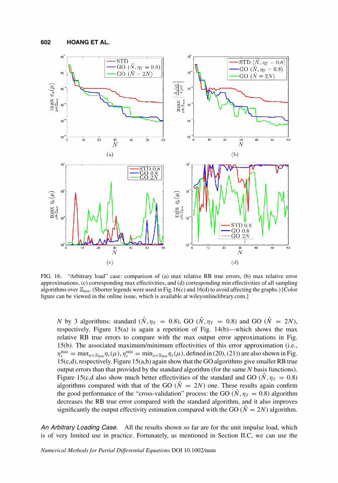
FIG. 16. “Arbitrary load” case: comparison of (a) max relative RB true errors, (b) max relative errorapproximations, (c) corresponding max effectivities, and (d) corresponding min effectivities of all samplingalgorithms over �test. (Shorter legends were used in Fig.16(c) and 16(d) to avoid affecting the graphs.) [Colorfigure can be viewed in the online issue, which is available at wileyonlinelibrary.com.]

N by 3 algorithms: standard (N , ηT = 0.8), GO (N , ηT = 0.8) and GO (N = 2N ),respectively. Figure 15(a) is again a repetition of Fig. 14(b)—which shows the maxrelative RB true errors to compare with the max output error approximations in Fig.15(b). The associated maximum/minimum effectivities of this error approximation (i.e.,ηmax

s = maxμ∈�testηs(μ), ηmins = minμ∈�testηs(μ), defined in (20), (21)) are also shown in Fig.

15(c,d), respectively. Figure 15(a,b) again show that the GO algorithms give smaller RB trueoutput errors than that provided by the standard algorithm (for the same N basis functions).Figure 15(c,d also show much better effectivities of the standard and GO (N , ηT = 0.8)algorithms compared with that of the GO (N = 2N ) one. These results again confirmthe good performance of the “cross-validation” process: the GO (N , ηT = 0.8) algorithmdecreases the RB true error compared with the standard algorithm, and it also improvessignificantly the output effectivity estimation compared with the GO (N = 2N ) algorithm.

An Arbitrary Loading Case. All the results shown so far are for the unit impulse load, whichis of very limited use in practice. Fortunately, as mentioned in Section II.C, we can use the



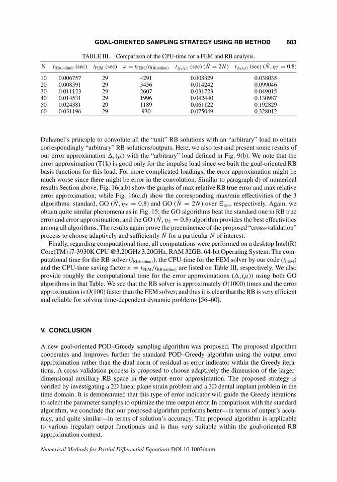
TABLE III. Comparison of the CPU-time for a FEM and RB analysis.

N tRB(online) (sec) tFEM (sec) κ = tFEM/tRB(online) t�s (μ) (sec) (N = 2N ) t�s (μ) (sec) (N , ηT = 0.8)

10 0.006757 29 4291 0.008329 0.03803520 0.008391 29 3456 0.014242 0.09904630 0.011123 29 2607 0.031723 0.04901540 0.014531 29 1996 0.042440 0.13098750 0.024381 29 1189 0.061122 0.19282960 0.031196 29 930 0.075049 0.328012

Duhamel’s principle to convolute all the “unit” RB solutions with an “arbitrary” load to obtaincorrespondingly “arbitrary” RB solutions/outputs. Here, we also test and present some results ofour error approximation �s(μ) with the “arbitrary” load defined in Fig. 9(b). We note that theerror approximation (T1k) is good only for the impulse load since we built the goal-oriented RBbasis functions for this load. For more complicated loadings, the error approximation might bemuch worse since there might be error in the convolution. Similar to paragraph d) of numericalresults Section above, Fig. 16(a,b) show the graphs of max relative RB true error and max relativeerror approximation; while Fig. 16(c,d) show the corresponding max/min effectivities of the 3algorithms: standard, GO (N , ηT = 0.8) and GO (N = 2N ) over �test, respectively. Again, weobtain quite similar phenomena as in Fig. 15: the GO algorithms beat the standard one in RB trueerror and error approximation; and the GO (N , ηT = 0.8) algorithm provides the best effectivitiesamong all algorithms. The results again prove the preeminence of the proposed “cross-validation”process to choose adaptively and sufficiently N for a particular N of interest.

Finally, regarding computational time, all computations were performed on a desktop Intel(R)Core(TM) i7-3930K CPU @3.20GHz 3.20GHz, RAM 32GB, 64-bit Operating System. The com-putational time for the RB solver (tRB(online)), the CPU-time for the FEM solver by our code (tFEM)and the CPU-time saving factor κ = tFEM/tRB(online) are listed on Table III, respectively. We alsoprovide roughly the computational time for the error approximations (�s(μ)) using both GOalgorithms in that Table. We see that the RB solver is approximately O(1000) times and the errorapproximation is O(100) faster than the FEM solver; and thus it is clear that the RB is very efficientand reliable for solving time-dependent dynamic problems [56–60].

V. CONCLUSION

A new goal-oriented POD–Greedy sampling algorithm was proposed. The proposed algorithmcooperates and improves further the standard POD–Greedy algorithm using the output errorapproximation rather than the dual norm of residual as error indicator within the Greedy itera-tions. A cross-validation process is proposed to choose adaptively the dimension of the larger-dimensional auxiliary RB space in the output error approximation. The proposed strategy isverified by investigating a 2D linear plane strain problem and a 3D dental implant problem in thetime domain. It is demonstrated that this type of error indicator will guide the Greedy iterationsto select the parameter samples to optimize the true output error. In comparison with the standardalgorithm, we conclude that our proposed algorithm performs better—in terms of output’s accu-racy, and quite similar—in terms of solution’s accuracy. The proposed algorithm is applicableto various (regular) output functionals and is thus very suitable within the goal-oriented RBapproximation context.


604 HOANG ET AL.

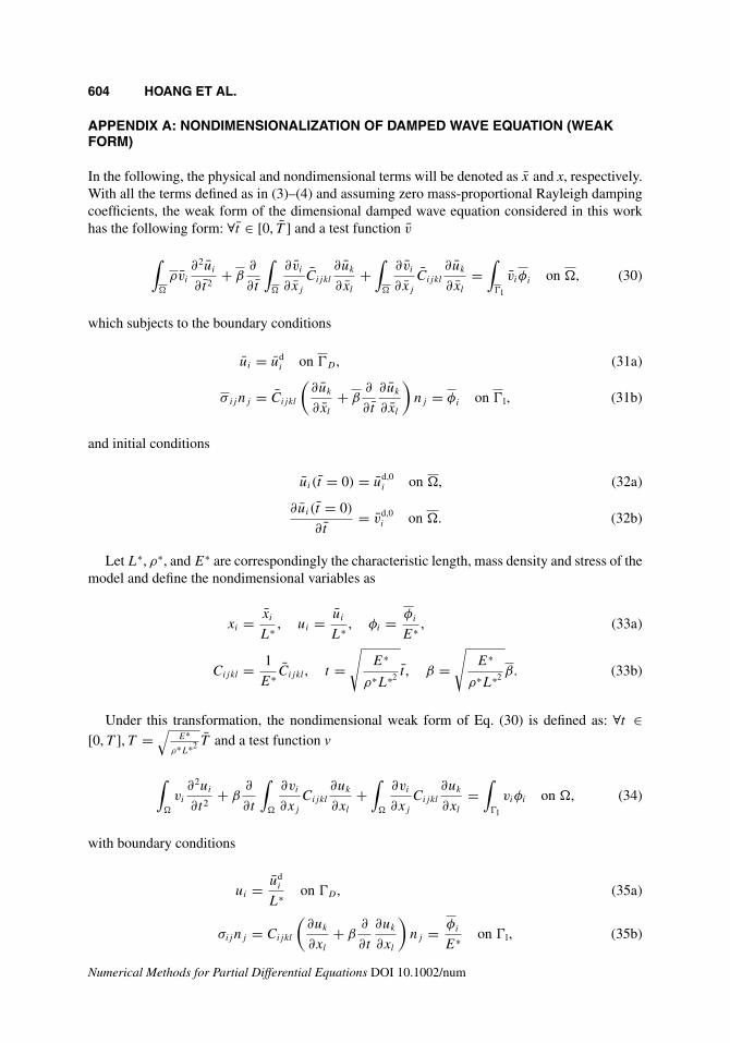
APPENDIX A: NONDIMENSIONALIZATION OF DAMPED WAVE EQUATION (WEAKFORM)

In the following, the physical and nondimensional terms will be denoted as x and x, respectively.With all the terms defined as in (3)–(4) and assuming zero mass-proportional Rayleigh dampingcoefficients, the weak form of the dimensional damped wave equation considered in this workhas the following form: ∀t ∈ [0, T ] and a test function v

∫�

ρvi

∂2ui

∂ t2+ β

∂

∂t

∫�

∂vi

∂xj

Cijkl

∂uk

∂xl

+∫

�

∂vi

∂xj

Cijkl

∂uk

∂xl

=∫

�l

viφi on �, (30)

which subjects to the boundary conditions

ui = udi on �D , (31a)

σ ijnj = Cijkl

(∂uk

∂xl

+ β∂

∂t

∂uk

∂xl

)nj = φi on �l, (31b)

and initial conditions

ui(t = 0) = ud,0i on �, (32a)

∂ui(t = 0)

∂t= v

d,0i on �. (32b)

Let L∗, ρ∗, and E∗ are correspondingly the characteristic length, mass density and stress of themodel and define the nondimensional variables as

xi = xi

L∗ , ui = ui

L∗ , φi = φi

E∗ , (33a)

Cijkl = 1

E∗ Cijkl , t =√

E∗

ρ∗L∗2 t , β =√

E∗

ρ∗L∗2 β. (33b)

Under this transformation, the nondimensional weak form of Eq. (30) is defined as: ∀t ∈[0, T ], T =

√E∗

ρ∗L∗2 T and a test function v

∫�

vi

∂2ui

∂t2+ β

∂

∂t

∫�

∂vi

∂xj

Cijkl

∂uk

∂xl

+∫

�

∂vi

∂xj

Cijkl

∂uk

∂xl

=∫

�l

viφi on �, (34)

with boundary conditions

ui = udi

L∗ on �D , (35a)

σijnj = Cijkl

(∂uk

∂xl

+ β∂

∂t

∂uk

∂xl

)nj = φi

E∗ on �l, (35b)



and initial conditions

ui(t = 0) = ud,0i

L∗ on �, (36a)

∂ui(t = 0)

∂t=

√ρ∗

E∗ vd,0i on �. (36b)

The authors also thank the anonymous reviewers for many contributive comments whichimprove the quality of this article.

References

1. L. Sirovich, Turbulence and the dynamics of coherent structures, part 1: Coherent structures, Q ApplMath 45 (1987), 561–571.

2. P. Kerfriden, P. Gosselet, S. Adhikari, S. Bordas, and J.-C. Passieux, POD-based model order reductionfor the simulation of strong nonlinear evolutions in structures: Application to damage propagation, IOPConf Ser: Mater Sci Eng 10 (2010), 012165.

3. P. Kerfriden, J.-C. Passieux, and S. P.-A. Bordas, Local/global model order reduction strategy for thesimulation of quasi-brittle fracture, Int J Numer Methods Eng 89 (2011), 154–179.

4. P. Kerfriden, P. Gosselet, S. Adhikari, and S. P.-A. Bordas, Bridging proper orthogonal decomposi-tion methods and augmented Newton–Krylov algorithms: an adaptive model order reduction for highlynonlinear mechanical problems, Comput Methods Appl Mech Eng 200 (2011), 850–866.

5. P. Kerfriden, O. Goury, T. Rabczuk, and S. P.-A. Bordas, A partitioned model order reduction approachto rationalise computational expenses in nonlinear fracture mechanics, Comput Methods Appl MechEng 256 (2012), 169–188.

6. P. Kerfriden, J. J. Rodenas, and S. P. A. Bordas, Certification of projection-based reduced order model-ling in computational homogenisation by the constitutive relation error, Int J Numer Methods Eng 97(2014), 395–422.

7. G. Rozza, D. B. P. Huynh, and A. T. Patera, Reduced basis approximation and a posteriori error esti-mation for affinely parametrized elliptic coercive partial differential equations, Arch Comput MethodsEng 15 (2008), 229–275.

8. K. C. Hoang, B. C. Khoo, G. R. Liu, N. C. Nguyen, and A. T. Patera, Rapid identification of materialproperties of the interface tissue in dental implant systems using reduced basis method, Inverse ProblSci Eng 21 (2013), 1310–1334.

9. A. K. Noor and J. M. Peters, Reduced basis technique for nonlinear analysis of structures, AIAA J 18(1980), 455–462.

10. L. Machiels, Y. Maday, I. B. Oliveira, A. T. Patera, and D. V. Rovas, Output bounds for reduced-basisapproximations of symmetric positive definite eigenvalue problems, Comptes Rendus de l’Académiedes Sciences-Series I-Mathematics 331 (2000), 153–158.

11. K. Veroy, C. Prudhomme, D. V. Rovas, and A. T. Patera, A posteriori error bounds for reduced-basisapproximation of parametrized noncoercive and nonlinear elliptic partial differential equations, In: Pro-ceedings of the 16th AIAA Computational Fluid Dynamics Conference, Vol. 3847, 23–26 June 2003,Orlando, Florida.

12. M. A. Grepl and A. T. Patera, A posteriori error bounds for reduced-basis approximations of parametrizedparabolic partial differential equations, ESAIM: Math Model Numer Anal 39 (2005), 157–181.

13. M. A. Grepl, Y. Maday, N. C. Nguyen, and A. T. Patera, Efficient reduced-basis treatment of nonaffineand nonlinear partial differential equations, ESAIM: Math Model Numer Anal 41 (2007), 575–605.

14. A. Y. K. Tan, Reduced basis method for 2nd order wave equation: Application to one-dimensionalseismic problem, Master’s Thesis, Massachusetts Institute of Technology, 2007.


606 HOANG ET AL.

15. N.-C. Nguyen, G. Rozza, and A. T. Patera, Reduced basis approximation and a posteriori error estimationfor the time-dependent viscous Burgers equation, Calcolo 46 (2009), 157–185.

16. N. Jung, B. Haasdonk, and D. Kroner, Reduced basis method for quadratically nonlinear transportequations, Int J Comput Sci Math 2 (2009), 334–353.

17. D. J. Knezevic, N.-C. Nguyen, and A. T. Patera, Reduced basis approximation and a posteriori errorestimation for the parametrized unsteady Boussinesq equations, Math Model Methods Appl Sci 21(2011), 1415–1442.

18. D. B. P. Huynh, D. J. Knezevic, and A. T. Patera, A Laplace transform certified reduced basis method;application to the heat equation and wave equation, Comptes Rendus Mathematique 349 (2011),401–405.

19. K. C. Hoang, Reduced basis approximation and inverse analyses for dental implant problems, PhDThesis, Singapore–MIT Alliance, National University of Singapore, 2012.

20. T. Grätsch and K.-J. Bathe, A posteriori error estimation techniques in practical finite element analysis,Comput Struct 83 (2005), 235–265.

21. P. Ladevèze, F. Pled, and L. Chamoin, New bounding techniques for goal-oriented error estimationapplied to linear problems, Int J Numer Methods Eng 93 (2012), 1345–1380.

22. M. Rüter and E. Stein, Goal-oriented a posteriori error estimates in linear elastic fracture mechanics,Comput Methods Appl Mech Eng 195 (2006), 251–278.

23. O. A. González-Estrada, J. J. Ródenas, S. P. A. Bordas, M. Duflot, P. Kerfriden, and E. Giner, On therole of enrichment and statistical admissibility of recovered fields in a-posteriori error estimation forenriched finite element methods, Eng Comput 29 (2012), 814–841.

24. O. A. González-Estrada, E. Nadal, J. J. Ródenas, P. Kerfriden, S. P. A. Bordas, and F. J. Fuenmayor,Mesh adaptivity driven by goal-oriented locally equilibrated superconvergent patch recovery, ComputMech 53 (2014), 957–976.

25. F. Larsson, K. Runesson, and P. Hansbo, Computation of goal-oriented a posteriori error measuresin space-time finite elements for viscoplasticity, In: W. Wall, K. -U. Bletzinger and K. Schweizerhof,editors, Trends in Computational Structural Mechanics, Int Center Numerical Methods Engineering,Barcelona, 2001, pp. 499–510.

26. S. P. A. Bordas and M. Duflot, Derivative recovery and a posteriori error estimate for extended finiteelements, Comput Methods Appl Mech Eng 196 (2007), 3381–3399.

27. M. Duflot and S. P. A. Bordas, A posteriori error estimation for extended finite elements by an extendedglobal recovery, Int J Numer Methods Eng 76 (2008), 1123–1138.

28. W. Bangerth and R. Rannacher, Finite element approximation of the acoustic wave equation: Errorcontrol and mesh adaptation, East West J Numer Math 7 (1999), 263–282.

29. W. Bangerth and R. Rannacher, Adaptive finite element techniques for the acoustic wave equation, JComput Acoust 9 (2001), 575–591.

30. R. Becker and R. Rannacher, An optimal control approach to a posteriori error estimation in finiteelement methods, Acta Numer 10 (2001), 1–102.

31. W. Bangerth, M. Geiger, and R. Rannacher, Adaptive Galerkin finite element methods for the waveequation, Comput Methods Appl Math 10 (2010), 3–48.

32. G. R. Liu, K. Zaw, and Y. Y. Wang, Rapid inverse parameter estimation using reduced-basisapproximation with asymptotic error estimation, Comput Methods Appl Mech Eng 197 (2008),3898–3910.

33. C. Prudhomme, D. V. Rovas, K. Veroy, L. Machiels, Y. Maday, A. T. Patera, and G. Turinici, Reliablereal-time solution of parametrized partial differential equations: Reduced-basis output bound methods,J Fluids Eng 124 (2002), 70–80.

34. P. Chen and A. Quarteroni, Accurate and efficient evaluation of failure probability for partial differentequations with random input data, Comput Methods Appl Mech Eng 267 (2013), 233–260.



35. K. Urban, S. Volkwein, and O. Zeeb, Greedy sampling using nonlinear optimization, In: Reduced ordermethods for modeling and computational reduction, Springer, Vol. 9, 2014, pp. 137–157.

36. M. Meyer and H. G. Matthies, Efficient model reduction in non-linear dynamics using the Karhunen-Loeve expansion and dual-weighted-residual methods, Comput Mech 31 (2003), 179–191.

37. T. Bui-Thanh, K. Willcox, O. Ghattas, and B. van Bloemen Waanders, Goal-oriented, model-constrainedoptimization for reduction of large-scale systems, J Comput Phys 224 (2007), 880–896.

38. K. Willcox, O. Ghattas, B. van Bloemen Waanders, and B. Bader, An optimization frame work for goal-oriented, model-based reduction of large-scale systems, In: 44th IEEE Conference on Decision andControl, 2005 and 2005 European Control Conference, CDC-ECC’05, 12–15 December 2005, Seville,Spain, pp. 2265–2271.

39. J. Nocedal and S. J. Wright, Numerical optimization, Vol. 2, Springer, New York, 1999.

40. M. Heinkenschloss, Numerical solution of implicitly constrained optimization problems, TechnicalReport, Rice University, Department of Computational and Applied Mathematics, 2008.

41. B. Haasdonk and M. Ohlberger, “Reduced basis method for finite volume approximations ofparametrized linear evolution equations,” ESAIM: Math Model Numer Anal 42 (2008), 277–302.

42. J. L. Lions, Optimal control of systems governed by partial differential equations, Printed in Germany,Springer, 1971.

43. K.-J. Bathe, Finite element procedures, by Prentice-Hall, Inc., New Jersey, 1996.

44. T. J. R. Hughes, The finite element method: Linear static and dynamic finite element analysis,Prentice-Hall International, Inc, Englewood Cliffs, New Jersey, 1987.

45. W. J. T. Daniel, The subcycled Newmark algorithm, Comput Mech 20 (1997), 272–281.

46. K. Zaw, G. R. Liu, B. Deng, and K. B. C. Tan, Rapid identification of elastic modulus of the interfacetissue on dental implants surfaces using reduced-basis method and a neural network, J Biomech 42(2009), 634–641.

47. S. Volkwein, Proper orthogonal decomposition: Theory and reduced-order modelling, Lecture Notes,University of Konstanz, 2013.

48. I. Jolliffe, Principal component analysis, Printed in the United States of America, Wiley, 2005.

49. N. C. Nguyen, A multiscale reduced-basis method for parametrized elliptic partial differential equationswith multiple scales, J Comput Phys 227 (2008), 9807–9822.

50. J. L. Eftang, D. J. Knezevic, and A. T. Patera, An hp certified reduced basis method for parametrizedparabolic partial differential equations, Math Comput Model Dyn Syst 17 (2011), 395–422.

51. B. Haasdonk, Convergence rates of the pod–greedy method, ESAIM: Math Model Numer Anal 47(2013), 859–873.

52. M. Yano, A. T. Patera, and K. Urban, A space-time certified reduced basis method for Burgers equation,Math Model Methods Appl Sci, Submitted, 2012.

53. M. Yano, A Space-Time Petrov–Galerkin certified reduced basis method: Application to the Boussinesqequations, SIAM J Sci Comput 36 (2014), A232–A266.

54. Y. Saad, Iterative methods for sparse linear systems, SIAM, Printed in the United States of America,2003.

55. S. Wang, G. R. Liu, K. C. Hoang, and Y. Guo, Identifiable range of osseointegration of dental implantsthrough resonance frequency analysis, Med Eng Phys 32 (2010), 1094–1106.

56. T. Rabczuk, S. P. A. Bordas, and G. Zi, A three-dimensional meshfree method for continuousmultiple-crack initiation, propagation and junction in statics and dynamics, Comput Mech 40 (2007),473–495.

57. J. H. Song, H. Wang, and T. Belytschko, A comparative study on finite element methods for dynamicfracture, Comput Mech 42 (2008), 239–250.


608 HOANG ET AL.

58. T. Rabczuk, S. P. A. Bordas, and G. Zi, On three-dimensional modelling of crack growth using partitionof unity methods, Comput Struct 88 (2010), 1391–1411.

59. H. Nguyen-Vinh, I. Bakar, M. A. Msekh, J.-H. Song, J. Muthu, G. Zi, P. Le, et al., Extended finiteelement method for dynamic fracture of piezo-electric materials, Eng Fract Mech 92 (2012), 19–31.

60. N. Nguyen-Thanh, T. Rabczuk, H. Nguyen-Xuan, and S. P. A. Bordas, An alternative alpha finite ele-ment method (AαFEM) for free and forced structural vibration using triangular meshes, J Comput ApplMath 233 (2010), 2112–2135.


An efficient goal-oriented sampling strategy using reduced basis method for parametrized elastodynamic problems

Documents