An Efficient Algorithm for Statistical Multiple Alignment on Arbitrary Phylogenetic Trees

JOURNAL OF COMPUTATIONAL BIOLOGYVolume 10, Number 6, 2003© Mary Ann Liebert, Inc.Pp. 869–889

An Ef� cient Algorithm for Statistical MultipleAlignment on Arbitrary Phylogenetic Trees

G.A. LUNTER, I. MIKLÓS, Y.S. SONG, and J. HEIN

ABSTRACT

We present an ef� cient algorithm for statistical multiple alignment based on the TKF91model of Thorne, Kishino, and Felsenstein (1991) on an arbitrary k-leaved phylogenetictree. The existing algorithms use a hidden Markov model approach, which requires at least

O.p

5k/ states and leads to a time complexity of O.5kLk/, where L is the geometric mean

sequence length. Using a combinatorial technique reminiscent of inclusion/exclusion, we areable to sum away the states, thus improving the time complexity to O.2kLk/ and consid-erably reducing memory requirements. This makes statistical multiple alignment under theTKF91 model a de� nite practical possibility in the case of a phylogenetic tree with a modestnumber of leaves.

Key words: statistical alignment, multiple alignment, phylogeny, maximum likelihood.

1. INTRODUCTION

Amajor way by which biological sequences evolve is mutation. Three main types of mutationevents are substitutions, insertions, and deletions of amino acids or nucleotides. The latter two events,

insertions and deletions, introduce the problem of aligning sequences, so that homologous positions appearin the same column of an alignment. When the aim is to � nd sequences from a database which arehomologous to a query sequence, current alignment techniques perform quite well. The alignment problemin phylogenetics, however, is still a serious challenge (Lee, 2001; Goldman, 1998). For example, thephylogenies inferred from different, but equally good, alignments can be quite different (Goldman, 1998).Some researchers have suggested that the regions in the sequences which are responsible for this variancein the inferred phylogeny (usually referred to as unalignable regions [Lee, 2001]) should be omitted. It isunclear, however, how much information is lost by ignoring such regions. Moreover, several studies havesuggested that accurate evolutionary parameters cannot be obtained using only a single “best” alignment(Thorne et al., 1991; Hein et al., 2000), even if this alignment is seemingly reliable (Hein et al., 2000).A more robust approach is to take into account all possible alignments, or a large subset of those, in astatistical framework.

Since insertions and deletions, like substitutions, are rare random events, it seems natural to model themby a continuous time stochastic process, with rates for the three types of mutations. Stochastic models

Department of Statistics, University of Oxford, Oxford, OX1 3TG, UK.

869

870 LUNTER ET AL.

for the substitution process are well known and widely used to obtain maximum-likelihood evolutionaryparameters (Felsenstein, 1981; Whelan et al., 2001). The model of Thorne, Kishino, and Felsenstein (theTKF91 model, hereafter) of sequence evolution incorporates such a mutation model, and moreover allows anucleotide to spawn new nucleotides adjacent to itself, and to die. To model evolution on a phylogenetic tree,the TKF91 model is applied to each branch of the tree, and likelihood calculation of multiple alignmentsthen becomes possible.

Since the TKF91 model is reversible (and the sequence distribution at the root is assumed to be atequilibrium), the root placement is immaterial. In the case of two sequences, one of the sequences maytherefore be considered the ancestral sequence and the other its descendant. In that framework, the numberof possible alignments is � nite. When the TKF91 model is applied to a tree, however, an in� nite numberof sequences may appear at internal nodes, for any given set of sequences which appear at the leaf nodes.Thus, such an extension is not straightforward, and several methods have been proposed. For star-shapedtrees, Steel and Hein (2001) have constructed an algorithm with O.L2k/ running time for k sequences withgeometric mean length L, and it has subsequently been extended, with similar time complexity, to binarytrees (Hein, 2001). Thenceforth, the time complexity has been reduced to O.4kLk/ for star-shaped trees(Miklós, 2002) and to O.5kLk/ for arbitrary binary trees (Hein et al., 2002) (see Appendix B). In the latterpaper, the TKF91 model has been reformulated as a multiple hidden Markov model, in which likelihoodcalculations can be performed using forward and backward algorithms known in the HMM literature(Durbin et al., 1998). Similar ideas have appeared for pairwise and triplewise statistical alignment as well,e.g., Holmes and Bruno (2001) give HMM formulations for alignment on two- and three-leaved trees and

use it for sampling larger trees. In the Markov models, there are O.p

5k/ states, and therefore the running

time of these algorithms is indeed O.5kLk/, in accordance with the general theory of HMMs (Durbin

et al., 1998). The memory usage is of the order O.p

5kLk/ if the entire dynamic programming table is

retained and O.p

5kLk¡1/ if not (Hirshberg, 1977).

Because of the large number of states, the aforementioned algorithms are quite slow, even for a moderatenumber of sequences. Hein et al. (2000), however, have developed an algorithm for statistical alignment oftwo sequences which needs neither different states of a HMM nor partition of probabilities into differenttypes of alignments (Thorne et al., 1991). This is in contrast to the original formulation of the TKF91model, which uses three states. The algorithm of Hein et al. (2000) is, both in time and space complexity,as simple as the traditional distance- or similarity-based dynamic programming algorithms (Needlemanand Wunsch, 1970; Sankoff and Kruskall, 1983). Henceforward, we refer to it as the one-state recursion.

In this paper, we present a one-state recursion for statistical alignment on arbitrary phylogenetic trees.Essentially, it combines the idea of Hein et al. (2000) generalized to trees and Felsenstein’s reverse traversalalgorithm (1981). The � rst idea allows us to reduce the number of states to one, and the second to computein linear time the exponential number of terms that occur in the transition factors. The resulting algorithmhas time complexity O.2kLk/ and space complexity O.Lk/ if the entire dynamic programming table isstored in memory, O.Lk¡1/ if not. This represents a great saving in both space and time compared tothe hidden Markov recursion and makes statistical alignment on a phylogenetic tree of modest size ade� nite practical possibility. Indeed, we have implemented both methods for three and four sequences andachieved a considerable acceleration. One of us (IM) was able to perform a likelihood ratio test (Felsenstein,1981; Whelan et al., 2001) for more than 250 triplets of yeast protein sequences in a day, using triplewisestatistical alignments. Moreover, this one-state recursion can be coupled with corner-cutting techniques(Hein et al., 2000), which provides further reduction both in time and space complexity.

The organization of this paper is as follows. We brie� y describe the TKF model in Section 2 and discussin Section 3 the one-state recursion in the case of two sequences. The two-sequence example is simple,but well illustrates our general approach. We discuss in Section 4 our algorithm for the one-state recursionand consider a speci� c application in Section 5. The main ideas underlying our proof are sketched inSection 6. The general one-state recursion is described in Section 7 and the computation of the transitionfactors which occur in the recursion is discussed in Section 8. In Appendix C we draw a connection witha hidden Markov model and describe how optimal alignments can be obtained. We conclude with someremarks and discussion in Section 9. In the appendix, we show that the number of Markov states in the

HJP recursion is O.p

5k/ and give a proof of Lemma 1 from Section 7.

AN ALGORITHM FOR STATISTICAL MULTIPLE ALIGNMENT 871

2. THE TKF MODEL

The TKF91 model is a continuous time reversible Markov model for the evolution of nucleotide (oramino acid) sequences. It models three of the main processes in sequence evolution, namely substitutions,insertions, and deletions of nucleotides, approximating these as single-nucleotide processes. A nucleotidesequence is represented by an alternating string of nucleotides and links connecting the nucleotides, andthis string both starts and terminates with a link. We adopt the view that insertions originate from links andadd a nucleotide–link pair to the right of the original link; deletions originate from nucleotides and havethe effect of removing the nucleotide and its right link. (This view is slightly different but equivalent to theoriginal description; see Thorne et al. [1991].) In this way, nucleotide subsequences evolve independentlyof each other, and the evolution of a nucleotide sequence is the sum of the evolutions of individualnucleotide–link pairs. The leftmost link of the sequence has no corresponding nucleotide to its left; hence,it is never deleted, and for this reason it is called the immortal link.

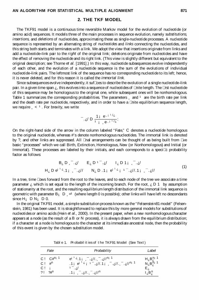
Since subsequences evolve independently, it suf� ces to describe the evolution of a single nucleotide–linkpair. In a given time span ¿ , this evolves into a sequence of nucleotides of � nite length. The � rst nucleotideof this sequence may be homologous to the original one, while subsequent ones will be nonhomologous.Table 1 summarizes the corresponding probabilities. The parameters ¸ and ¹ are the birth rate per linkand the death rate per nucleotide, respectively, and in order to have a � nite equilibrium sequence length,we require ¸ < ¹. For brevity, we write

¯.¿/ D 1 ¡ e.¸¡¹/¿

¹ ¡ ¸e.¸¡¹/¿:

On the right-hand side of the arrow in the column labeled “Fate,” C denotes a nucleotide homologousto the original nucleotide, whereas #’s denote nonhomologous nucleotides. The immortal link is denotedby ?, and other links are suppressed. All � nal arrangements can be thought of as being built from � vebasic “processes” which we call Birth, Extinction, Homologous, New (or Nonhomologous) and Initial (orImmortal). These processes are labeled by their initials, and each corresponds to a speci� c probabilityfactor as follows:

B¿ D ¸¯.¿/ E¿ D ¹¯.¿/ I¿ D 1 ¡ ¸¯.¿/

H¿ D e¡¹¿ .1 ¡ ¸¯.¿// N¿ D .1 ¡ e¡¹¿ ¡ ¹¯.¿//.1 ¡ ¸¯.¿//(1)

In a tree, time � ows forward from the root to the leaves, and to each node of the tree we associate a timeparameter ¿ which is set equal to the length of the incoming branch. For the root, ¿ D 1 by assumptionof stationarity at the root, and the resulting equilibrium length distribution of the immortal link sequence isgeometric with parameter B1 D ¸=¹ (where length 0 is possible); other links will have left no descendantssince H1 D N1 D 0.

In the original TKF91 model, a simple substitution process known as the “Felsenstein81 model” (Felsen-stein, 1981) has been used. It is straightforward to replace this by more general models for substitutions ofnucleotides or amino acids (Hein et al., 2000). In the present paper, when a new nonhomologous characterappears at a node (as the result of a B or N process), it is always drawn from the equilibrium distribution;if a character at a node is homologous to the character at its immediate ancestral node, then the probabilityof this event is given by the chosen substitution model.

Table 1. Probabilities of the TKF91 Model (See Text)

Fate Probability Label

C ! C#n¡1 e¡¹¿ .1 ¡ ¸¯.¿ //.¸¯.¿//n¡1 H¿ Bn¡1¿

C ! #n .1 ¡ e¡¹¿ ¡ ¹¯.¿ //.1 ¡ ¸¯.¿ //.¸¯.¿//n¡1 N¿ Bn¡1¿

C ! ¡ ¹¯.¿/ E¿

? ! ?#n .1 ¡ ¸¯.¿ //.¸¯.¿//n I¿ Bn¿

872 LUNTER ET AL.

Note that we do not sum over possible alignments, but over what we call evolutionary histories (seesection 7.1), which is a discrete summary of the actual evolutionary events in the model specifying thefate of all ancestral nucleotides. As was pointed out by Thorne et al. (1991), for two sequences, there isalmost a correspondence between alignment and evolutionary history (except that gaps in two sequencesthat immediately follow each other may be interchanged without changing the interpretation as alignmentswhereas the evolutionary interpretation in the TKF model is different.) This almost-correspondence breaksdown for trees with larger number of leaves, since information on what occurs at internal nodes is lost inan alignment, which only records the homology structure of observed nucleotides.

3. ONE-STATE RECURSION: A GRAPHICAL PROOF FOR TWO SEQUENCES

Hein et al. (2000) give a proof for the one-state recursion in the case of two-sequence alignment. Herewe provide a different proof for this particular case. Our proof for the general case follows a similar lineof ideas.

Suppose A1 is the ancestral sequence observed at the root and A2 is the descendant sequence whichresults from the TKF91 process after time ¿ . Let Ak

i (respectively, aki ) denote the i-long pre� x (respectively,

the ith character) of sequence Ak . Let P .i; j/ be the joint probability of observing A1i and A2

j . Given thatP .i ¡ 1; j /, P .i; j ¡ 1/, and P .i ¡ 1; j ¡ 1/ are known, we want to compute P .i; j/.

The possible evolutionary histories (or alignments) are customarily (Thorne et al., 1991) classi� ed intothree groups, S0, S1, and S2, according to whether the rightmost root link has 0, 1, or at least 2 descendantsat the leaf. Another way to de� ne these sets is by the last columns in the alignment; symbolically, S0 D f #

¡ g,S1 D f #

# ; #¡

¡# g, and S2 D f #

#¡# ; ¡

#¡# g, where the upper symbols represent nucleotides at the root. These

sets are associated to the evolutionary processes as follows. After the B1E¿ process, the rightmost rootlink has 0 descendants, so the history is in f #

¡ g. After B1H¿ or B1N¿ , it is in f ## ; #

¡¡# g, while after a

birth at the leaf node (B¿ ), the alignment ends in either of f ##

¡# ; ¡

#¡# g. These processes may happen in any

order, except that a transition from f #¡ g to f #

#¡# ; ¡

#¡# g is not allowed: new births at the leaf (B¿ processes)

are allowed except after an extinction (E¿ ) process; see Table 1. A graphical depiction of the three-staterecursion that implements this restriction is provided in Fig. 1. The labeled circle segment representsprobabilities of observing the associated sequence pre� xes, provided the alignment ends according to thelabeling.

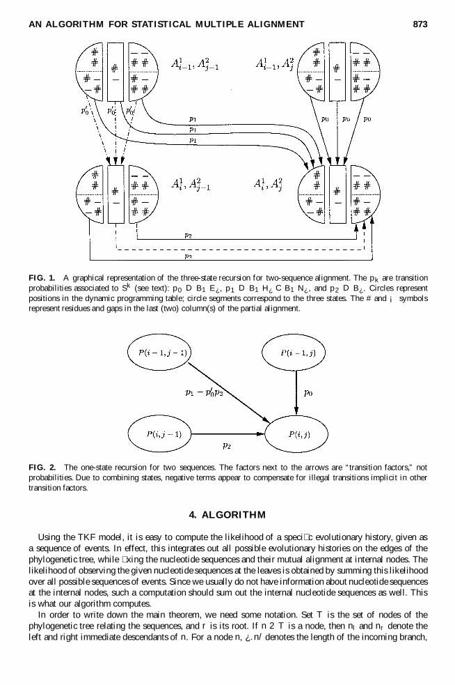
If we combine the three states at each position, by summing their probabilities, we can still computethe contribution of the vertical and diagonal transitions to the probabilities at .i; j /, since the transitionprobabilities (p0 and p1) do not depend on the state. But, for the horizontal transition we would includea contribution from the illegal transition f #

¡ g ! f ##

¡# ; ¡

#¡# g (denoted by a dashed arrow), leading to an

overestimation of the probability at .i; j /. This overestimation can be exactly corrected for, however, sincethe segment labeled #

¡ at .i; j ¡ 1/ is the result of a B1E¿ process from position .i ¡ 1; j ¡ 1/ (thedot-dashed arrows in Fig. 1). In summary, if we let P .i; j / be the sum of the three conditional probabilitiesat .i; j/, we obtain the following one-state recursion:

P .i; j / D P .i ¡ 1; j / £ B1¼.a1i /E¿

C P .i ¡ 1; j ¡ 1/ £ B1¼.a1i /

hN¿ ¼.a2

j / C H¿ p.a1i ! a2

j /i

ChP .i; j ¡ 1/ ¡ P .i ¡ 1; j ¡ 1/B1¼.a1

i /E¿

i£ B¿ ¼.a2

j /:

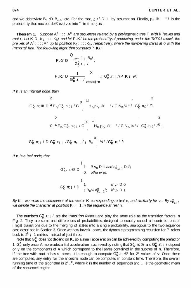
Here ¼.¢/ denotes the equilibrium nucleotide distribution, and p.® ! ° / is the probability that nucleotide® evolves into ° in time ¿ . After rearranging terms, we arrive at the recursion depicted in Fig. 2.

Although it is possible, in principle, to manually derive analogous recursions for an arbitrary number ofsequences following the same line of reasoning, such an approach rapidly gets very tedious, as the numberof terms which one needs to consider grows exponentially with the number of sequences. The goal of thepresent paper is to provide a more constructive method that allows us to prove that a one-state recursionindeed exists for arbitrary trees. Of more practical importance, the proof immediately suggests an ef� cientmethod for calculating the transition factors, through a post-order tree traversal algorithm, thus allowingcomputational derivation of the desired one-state recursion for arbitrary trees.


FIG. 1. A graphical representation of the three-state recursion for two-sequence alignment. The pk are transitionprobabilities associated to Sk (see text): p0 D B1E¿ , p1 D B1H¿ C B1N¿ , and p2 D B¿ . Circles representpositions in the dynamic programming table; circle segments correspond to the three states. The # and ¡ symbolsrepresent residues and gaps in the last (two) column(s) of the partial alignment.

FIG. 2. The one-state recursion for two sequences. The factors next to the arrows are “transition factors,” notprobabilities. Due to combining states, negative terms appear to compensate for illegal transitions implicit in othertransition factors.

4. ALGORITHM

Using the TKF model, it is easy to compute the likelihood of a speci� c evolutionary history, given asa sequence of events. In effect, this integrates out all possible evolutionary histories on the edges of thephylogenetic tree, while � xing the nucleotide sequences and their mutual alignment at internal nodes. Thelikelihood of observing the given nucleotide sequences at the leaves is obtained by summing this likelihoodover all possible sequences of events. Since we usually do not have information about nucleotide sequencesat the internal nodes, such a computation should sum out the internal nucleotide sequences as well. Thisis what our algorithm computes.

In order to write down the main theorem, we need some notation. Set T is the set of nodes of thephylogenetic tree relating the sequences, and r is its root. If n 2 T is a node, then nl and nr denote theleft and right immediate descendants of n. For a node n, ¿ .n/ denotes the length of the incoming branch,

874 LUNTER ET AL.

and we abbreviate Bn :D B¿.n/ etc. For the root, ¿ .r/ D 1 by assumption. Finally, pn.® ! ° / is theprobability that nucleotide ® evolves into ° in time ¿ .n/.

Theorem 1. Suppose A1; : : : ; Ak are sequences related by a phylogenetic tree T with k leaves androot r . Let K D .K1; : : : ; Kk/ and let P .K/ be the probability of producing, under the TKF91 model, thepre� xes of A1; : : : ; Ak up to position K1; : : : ; Kk , respectively, where the numbering starts at 0 with theimmortal link. The following algorithm computes P .K/:

P .0/ DQ

n2T .1 ¡ Bn/

G00.r; ¡/

;

P .K/ D 1

G0K.r; ¡/

X

v2f0;1gkn0

.¡GvK.r; ¡//P .K ¡ v/:

If n is an internal node, then

GvK.n; ®/ D

2

4EnlGv

K.nl; ¡/ CX

°

³Hnl

pnl.® ! ° / C Nnl

¼.° /

´Gv

K.nl ; ° /

3

5

£

2

4EnrGv

K.nr ; ¡/ CX

°

³Hnr

pnr.® ! ° / C Nnr

¼.° /

´Gv

K.nr ; ° /

3

5 ;

GvK.n; ¡/ D Gv

K.nl ; ¡/GvK.nr ; ¡/ ¡ Bn

X

°

¼.° /GvK.n; ° /:

If n is a leaf node, then

GvK.n; ®/ D

(1; if vn D 1 and an

Kn¡1 D ®,

0; otherwise.

GvK.n; ¡/ D

(1; if vn D 0,

¡Bn¼.anKn¡1/; if vn D 1.

By Kn , we mean the component of the vector K corresponding to leaf n, and similarly for vn. By anKn¡1

we denote the character at position Kn ¡ 1 in the sequence at leaf n.

The numbers GvK.r; ¡/ are the transition factors and play the same role as the transition factors in

Fig. 2. They are sums and differences of probabilities, designed to exactly cancel all contributions ofillegal transitions due to the merging of states into a single probability, analogous to the two-sequencecase described in Section 3. Since we now have k leaves, the dynamic programming recursion for P refersback to 2k ¡ 1 entries, instead of just three.

Note that G0K does not depend on K, so a small acceleration can be achieved by computing the prefactor

1=G0K only once. A more substantial acceleration is achieved by noting that Gv

K.n; ®/ and GvK.n; ¡/ depend

only on the components of v which correspond to the leaves contained in the subtree of n. Therefore,if the tree with root n has s leaves, it is enough to compute Gv

K.n; ®/ for 2s values of v. Once theseare computed, any entry for the ancestral node can be computed in constant time. Therefore, the overallrunning time of the algorithm is 2kLk , where k is the number of sequences and L is the geometric meanof the sequence lengths.


5. AN EXAMPLE

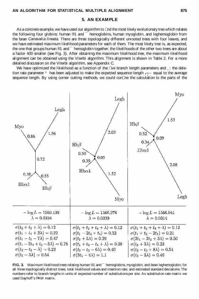
As a concrete example, we have used our algorithm to � nd the most likely evolutionary tree which relatesthe following four globins: human ®1 and ¯ hemoglobins, human myoglobin, and leghemoglobin fromthe bean Canavalia lineata. There are three topologically different unrooted trees with four leaves, andwe have estimated maximum likelihood parameters for each of them. The most likely tree is, as expected,the one that groups human ®1 and ¯ hemoglobin together; the likelihoods of the other two trees are abouta factor 400 smaller (see Fig. 3). After obtaining the maximum likelihood tree, the maximum likelihoodalignment can be obtained using the Viterbi algorithm. This alignment is shown in Table 2. For a moredetailed discussion on the Viterbi algorithm, see Appendix C.

We have optimized the likelihood as a function of the � ve branch length parameters and ¸; the dele-tion rate parameter ¹ has been adjusted to make the expected sequence length ¸

¹¡¸ equal to the averagesequence length. By using corner cutting methods, we could con� ne the calculation to the parts of the

FIG. 3. Maximum likelihood trees relating human ®1 and ¯ hemoglobins, myoglobin, and bean leghemoglobin, forall three topologically distinct trees; total likelihood values and insertion rate; and estimated standard deviations. Thenumbers refer to branch lengths in units of expected number of substitutions per site. As substitution rate matrix weused Dayhoff’s PAM matrix.

876 LUNTER ET AL.

Table 2. The Maximum Likelihood Alignment for the First Pedigree in Fig. 3a

Hba1: MV--LSPADKTNVKAAWGKVGAHAGEYGAEALERMFLSFPTTKTYFPHF--DLS-H-----GSAQVKGHGKKVAD-AL-TNA-Hbb: MV-HLTPEEKSAVTALWGKV--NVDEVGGEALGRLLVVYPWTQRFFESF-GDLSTPDAVM-GNPKVKAHGKKVLG-AF-SDG-Myo: MG--LSDGEWQLVLNVWGKVEADIPGHGQEVLIRLFKGHPETLEKFDKFK-HLKSEDE-MKASEDLKKHGATVLT-AL-GGI-Legh: MGA-FSEKQESLVKSSWEAFKQNVPHHSAVFYTLILEKAPAAQNMFS-F---LSNGVD-P-NNPKLKAHAEKVFKMTVDSAVQ

VAHVDDMPNALSALSDLHAHKLRVDPVNFK-LLSHCLLVTLAAHLPAEFTPAVHASLDKFLASVSTVL-TS-K---YR-LAHLDNLKGTFATLSELHCDKLHVDPENFR-LLGNVLVCVLAHHFGKEFTPPVQAAYQKVVAGVANAL-AH-K---YH-LKKKGHHEAEIKPLAQSHATKHKI-PVKYLEFISECIIQVLQSKHPGDFGADAQGAMNKALELFRKDMASNYKELGFQGLRAKGEVVLADPTLGSVHVQKGVLDP-HFL-VVKEALLKTFKEAVGDKWNDELGNAWEVAYDELAAAI-KK-A-MGSA-

aThe log-likelihood of this alignment is ¡1593:223.

dynamic programming table which contribute nonin� nitesimally to the � nal probability, resulting in aspeedup of about a factor of 500. At the extremal point we estimated the second derivative to get a co-variance matrix; see Fig. 3 for the standard deviations in the directions of the eigenvectors of this matrix.

6. IDEA OF PROOF

Our aim is to give a “one-state” dynamic programming algorithm for calculating the joint likelihoodof observing a set of sequences at the leaves of an evolutionary tree. This likelihood is the sum of theprobabilities of all evolutionary histories which produce the observed sequences at the leaves.

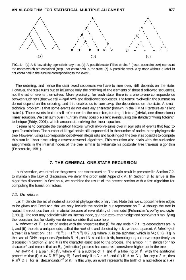
We introduce the concept of an event which corresponds to a nucleotidebirth at a node of the phylogenetictree and its subsequent fate down its descendant subtree. More precisely, in the process of going from onenode to a descendant node, one of the following three things may happen: The nucleotide may survive asa homologous nucleotide, it may die leaving at least one surviving new nucleotide, or it may go extinctaltogether. These three possibilities are labeled H, N, and E, respectively, as discussed in Section 2. In the� rst two cases, other nonhomologous descendants may have been born, but these possibilities are dealtwith in subsequent events. Hence, in this model, evolutionary histories of nucleotide sequences correspondto sequences of events. However, this correspondence is not one to one for two reasons. One reason is thatwe need to honor the TKF model, which does not allow extinct nucleotides to spawn new ones. (In Table 1,this is re� ected by the third entry, C ! ¡, which is the only one that may not be followed by a string of#’s.) The other reason is that different sequences of events may represent the same evolutionary history,since the relative ordering of events on disjoint subtrees has no meaning. In a Markov chain approach,these two requirements are met by de� ning states and by ruling out certain events (i.e., transitions, in theMealy machine view [Durbin et al., 1998]) in certain states. Essentially that is how we also approachthe problem. We de� ne a “state” and use it to rule out events which violate the TKF model. Our choiceof state (see Fig. 4) still allows overcounting of histories. To overcome this, we require the events to beordered in a speci� c way depending on the state.

The ordering we use has the property that in properly ordered sequences of events, an event whichviolates the TKF model can be recognized by comparing it to its immediate predecessor. This means thatwe do not need the state to decide which events are allowed, but the state is still used to de� ne the properordering. We can now use a recursion which, as a � rst approximation, allows all events. This includes alllegal sequences of events, as well as some sequences of events which end in an illegal pair, either becausethey are not properly ordered, or because they violate the TKF model. As a second approximation, wesubtract all sequences of events which end in particular illegal pairs. In the same way as before, thisincludes some illegal triplets which should not have been subtracted, and these are added in again, etc.,in a procedure reminiscent of inclusion–exclusion. We have dubbed the pairs, triplets, etc. involved in thisprocedure the disallowed sequences.

It turns out that there exist only � nitely many disallowed sequences, so that the inclusion–exclusion pro-cedure stops after � nitely many steps (bounded by the number of nodes in the tree). Moreover, disallowedsequences emit at most one nucleotide per leaf, and that leads to a recursion which refers back only to the2k ¡1 nearest predecessors in the k-dimensionaldynamic programming table,where k is the number of leaves.


FIG. 4. (a) A 6-leaved phylogenetic binary tree. (b) A possible state. Filled circles ² (resp., open circles ±) representthe nodes which are contained (resp., not contained) in the state. (c) A possible event. Any node without a label isnot contained in the subtree corresponding to the event.

The ordering, and hence the disallowed sequences we have to sum over, still depends on the state.However, the state turns out to in� uence only the ordering of the elements of these disallowed sequences,not the set of events themselves. More precisely, for each state, there is a one-to-one correspondencebetween such sets (that we call illegal sets) and disallowed sequences. The terms involved in the summationdo not depend on the ordering, and this enables us to sum away the dependence on the state. A smalltechnical problem is that some events do not emit any character (known in the HMM literature as “silentstates”). These events lead to self-references in the recursion, turning it into a (trivial, one-dimensional)linear equation. We can sum over in� nitely many possible silent events using the standard “wing folding”technique (Eddy, 2001), which amounts to solving the linear equation.

It remains to compute the transition factors, which involve sums over illegal sets of events that lead tospeci� c emissions. The number of illegal sets is still exponential in the number of nodes in the phylogenetictree. However, using a correspondence between illegal sets and labelings of the tree, it is possible to computethis sum in linear time using a reverse-traversal algorithm. This recursion also deals with the nucleotideassignments in the internal nodes of the tree, similar to Felsenstein’s postorder tree traversal algorithm(Felsenstein, 1981).

7. THE GENERAL ONE-STATE RECURSION

In this section, we introduce the general one-state recursion. The main result is presented in Section 7.2;to maintain the � ow of discussion, we defer the proof until Appendix A. In Section 8, to arrive at thealgorithm discussed in Section 4, we combine the result of the present section with a fast algorithm forcomputing the transition factors.

7.1. De� nitions

Let T denote the set of nodes of a rooted phylogenetic binary tree. Note that we suppose the tree edgesto be given and � xed and that we only include the nodes in our representation T . Although the tree isrooted, the root position is immaterial because of reversibility of the model (Felsenstein’s pulley principle,[1981]). The root may coincide with an internal node, giving a zero-length edge and somewhat simplifyingthe recursion, but for clarity we do not consider that case here.

A subtree t of T is a set of nodes with the properties that (i) for any node n 2 t , its descendants are int , and (ii) there is a unique node, called the root of t and denoted by r.t/, without a parent. A labeling ofa tree t is a function l : t ! fB®; ¡; H ® ; N ® j ® 2 Ag, where A is the alphabet, which is fA; C; G; T g inthe case of DNA sequences. Symbols B , H , and N stand for birth, homologous, and new, respectively, asdiscussed in Section 2, and ® is the character associated to the process. The symbol “¡” stands for “nocharacter” and means that an E¿ (extinction) process has occurred somewhere higher up in the tree.

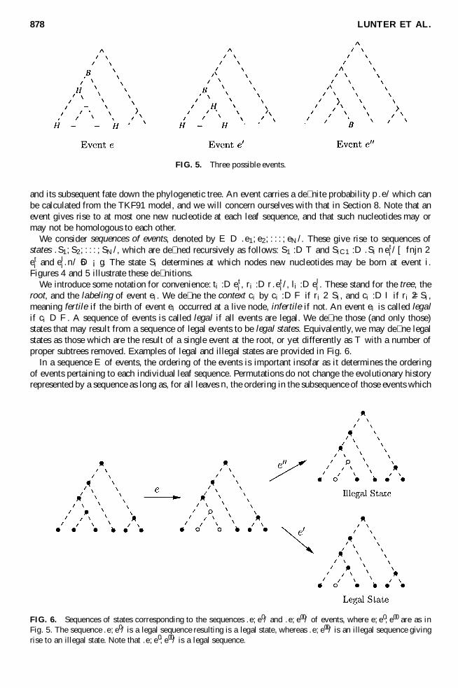
An event e is a pair .et ; el/, where et is a subtree of T and el a labeling of et , with the additionalproperties that (i) el.n/ D B® (any ®) if and only if n D r.et /, and (ii) if el.n/ D ¡ for any n 2 et , thenel.n0/ D ¡ for all descendants n0 of n. In this way, an event represents the birth of a nucleotide at r.et /

878 LUNTER ET AL.

FIG. 5. Three possible events.

and its subsequent fate down the phylogenetic tree. An event carries a de� nite probability p.e/ which canbe calculated from the TKF91 model, and we will concern ourselves with that in Section 8. Note that anevent gives rise to at most one new nucleotide at each leaf sequence, and that such nucleotides may ormay not be homologous to each other.

We consider sequences of events, denoted by E D .e1; e2; : : : ; eN /. These give rise to sequences ofstates .S1; S2; : : : ; SN /, which are de� ned recursively as follows: S1 :D T and SiC1 :D .Si n et

i/ [ fnjn 2et

i and eli.n/ 6D ¡g. The state Si determines at which nodes new nucleotides may be born at event i.

Figures 4 and 5 illustrate these de� nitions.We introduce some notation for convenience: ti :D et

i , ri :D r.eti/, li :D el

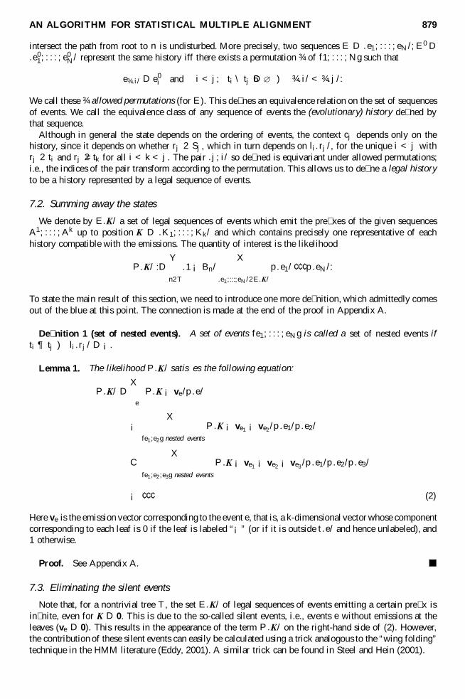
i . These stand for the tree, theroot, and the labeling of event ei . We de� ne the context ci by ci :D F if ri 2 Si , and ci :D I if ri =2 Si ,meaning fertile if the birth of event ei occurred at a live node, infertile if not. An event ei is called legalif ci D F . A sequence of events is called legal if all events are legal. We de� ne those (and only those)states that may result from a sequence of legal events to be legal states. Equivalently, we may de� ne legalstates as those which are the result of a single event at the root, or yet differently as T with a number ofproper subtrees removed. Examples of legal and illegal states are provided in Fig. 6.

In a sequence E of events, the ordering of the events is important insofar as it determines the orderingof events pertaining to each individual leaf sequence. Permutations do not change the evolutionary historyrepresented by a sequence as long as, for all leaves n, the ordering in the subsequence of those events which

FIG. 6. Sequences of states corresponding to the sequences .e; e0/ and .e; e00/ of events, where e; e0; e00 are as inFig. 5. The sequence .e; e0/ is a legal sequence resulting is a legal state, whereas .e; e00/ is an illegal sequence givingrise to an illegal state. Note that .e; e0; e00/ is a legal sequence.


intersect the path from root to n is undisturbed. More precisely, two sequences E D .e1; : : : ; eN /; E0 D.e0

1; : : : ; e0N / represent the same history iff there exists a permutation ¾ of f1; : : : ; Ng such that

e¾ .i/ D e0i and i < j; ti \ tj 6D ? ) ¾ .i/ < ¾.j/:

We call these ¾ allowed permutations (for E). This de� nes an equivalence relation on the set of sequencesof events. We call the equivalence class of any sequence of events the (evolutionary) history de� ned bythat sequence.

Although in general the state depends on the ordering of events, the context cj depends only on thehistory, since it depends on whether rj 2 Sj , which in turn depends on li.rj /, for the unique i < j withrj 2 ti and rj =2 tk for all i < k < j . The pair .j; i/ so de� ned is equivariant under allowed permutations;i.e., the indices of the pair transform according to the permutation. This allows us to de� ne a legal historyto be a history represented by a legal sequence of events.

7.2. Summing away the states

We denote by E.K/ a set of legal sequences of events which emit the pre� xes of the given sequencesA1; : : : ; Ak up to position K D .K1; : : : ; Kk/ and which contains precisely one representative of eachhistory compatible with the emissions. The quantity of interest is the likelihood

P .K/ :DY

n2T

.1 ¡ Bn/X

.e1;:::;eN /2E.K/

p.e1/ ¢ ¢ ¢ p.eN /:

To state the main result of this section, we need to introduce one more de� nition, which admittedly comesout of the blue at this point. The connection is made at the end of the proof in Appendix A.

De� nition 1 (set of nested events). A set of events fe1; : : : ; eN g is called a set of nested events ifti ¶ tj ) li.rj / D ¡.

Lemma 1. The likelihood P .K/ satis�es the following equation:

P .K/ DX

e

P .K ¡ ve/p.e/

¡X

fe1;e2g nested events

P .K ¡ ve1 ¡ ve2/p.e1/p.e2/

CX

fe1;e2;e3g nested events

P .K ¡ ve1 ¡ ve2 ¡ ve3 /p.e1/p.e2/p.e3/

¡ ¢ ¢ ¢ (2)

Here ve is the emission vector corresponding to the event e, that is, a k-dimensional vector whose componentcorresponding to each leaf is 0 if the leaf is labeled “¡” (or if it is outside t .e/ and hence unlabeled), and1 otherwise.

Proof. See Appendix A.

7.3. Eliminating the silent events

Note that, for a nontrivial tree T , the set E.K/ of legal sequences of events emitting a certain pre� x isin� nite, even for K D 0. This is due to the so-called silent events, i.e., events e without emissions at theleaves (ve D 0). This results in the appearance of the term P .K/ on the right-hand side of (2). However,the contribution of these silent events can easily be calculated using a trick analogous to the “wing folding”technique in the HMM literature (Eddy, 2001). A similar trick can be found in Steel and Hein (2001).

880 LUNTER ET AL.

Note that by de� nition, the set feg is a set of nested events, and therefore (2) can be rewritten as follows:

P .K/ DX

M 6D ? nested events,

P±

K ¡P

ei2M vei

².¡1/jM jC1

Y

ei 2M

p.ei/: (3)

We can decompose the sum as

P .K/ DX

M 6D ? nested events,not all vei

D 0

P±

K ¡P

ei2M vei

².¡1/jM jC1

Y

ei 2M

p.ei/

C P .K/X

M 6D ? nested events,all vei D 0

.¡1/jM jC1Y

ei2M

p.ei/:

Solving this equation for P .K/ gives the correct answer and includes histories with 0; 1; 2; : : : silent events.A heuristic way to see this is to observe that the equation X D a C sX, where s and a are the silent andnonsilent contributions, respectively, is solved by X D a=.1 ¡ s/ D a.1 C s C s2 C ¢ ¢ ¢ /. This expansionclearly shows the separate contributions of chains of silent events of length 0; 1; 2; : : : . The reasoning inthe proof of Lemma 1 makes sure that only sequences of legal events are included, and that applies to thesilent states as well.

8. PRUNING THE TREE

In this section we shall present Theorem 1. The recursion (2) enables us to compute P .K/, but it requiressumming over a number of terms exponential in the number of sequences. A similar problem occurs whencalculating the likelihood of nucleotide emissions on a tree under a simple substitution model, in whichcase one needs to sum over an exponential number of nucleotide assignments to internal nodes. This canbe computed in linear time by Felsenstein’s linear time post-order tree traversal algorithm, which is againa dynamic programming algorithm, now on a tree instead of the more familiar square lattice. We proceedin a similar way, by � nding a correspondence between certain labelings of T and sets of nested events.The summation over all such labelings, including the .¡1/kC1 sign arising from the inclusion–exclusionargument, can be performed in linear time by a dynamic programming algorithm similar to Felsenstein’s.

The probability factor associated to an event is the product of conditional factors at the nodes of thephylogenetic tree, and the conditional factor at a node depends only on the labeling of the node and itsancestral node. The label determines both the process and the associated nucleotide, except for “¡” whichimplies an Extinction event only if its ancestral node is not labeled “¡”. Symbolically,

p.B®j¡/ D Bn¼.®/;

p.N® jX° / D Nn¼.®/; p.N®j¡/ D 0;

p.H® jX° / D Hnpn.° ! ®/; p.H ®j¡/ D 0;

p.¡jX° / D En; p.¡j¡/ D 1;

where ®; ° 2 A (c.f. Section 7.1). The symbol X, denoting the process in the ancestral node, may beanything except “¡”. The probability factors Bn, Nn , Hn , and En are subscripted with a node and arede� ned (c.f. (1)) in terms of the length of the incoming branch (1 if n D r.T /). Note that p.B®jX° / willnever occur.

This allows us to calculate probability factors of events, but we want to sum over nested events directly.It follows from De� nition 1 that for each node n 2 T , at most one event in the nested set has n labeledwith a symbol other than “¡”. Furthermore, since the roots of events are uniquely identi� ed as the onlynodes labeled B® , there is a one-to-one correspondence between sets of nested events and labelings of T


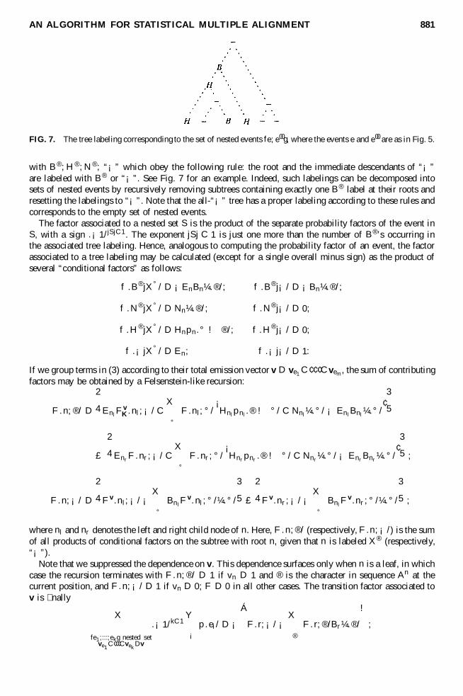
FIG. 7. The tree labeling corresponding to the set of nested events fe; e00g, where the events e and e00 are as in Fig. 5.

with B®; H ® ; N ®; “¡” which obey the following rule: the root and the immediate descendants of “¡”are labeled with B® or “¡”. See Fig. 7 for an example. Indeed, such labelings can be decomposed intosets of nested events by recursively removing subtrees containing exactly one B® label at their roots andresetting the labelings to “¡”. Note that the all-“¡” tree has a proper labeling according to these rules andcorresponds to the empty set of nested events.

The factor associated to a nested set S is the product of the separate probability factors of the event inS, with a sign .¡1/jSjC1. The exponent jSj C 1 is just one more than the number of B®’s occurring inthe associated tree labeling. Hence, analogous to computing the probability factor of an event, the factorassociated to a tree labeling may be calculated (except for a single overall minus sign) as the product ofseveral “conditional factors” as follows:

f .B® jX° / D ¡EnBn¼.®/; f .B® j¡/ D ¡Bn¼.®/;

f .N® jX° / D Nn¼.®/; f .N® j¡/ D 0;

f .H® jX° / D Hnpn.° ! ®/; f .H® j¡/ D 0;

f .¡jX° / D En; f .¡j¡/ D 1:

If we group terms in (3) according to their total emission vector v D ve1 C¢ ¢ ¢Cvem , the sum of contributingfactors may be obtained by a Felsenstein-like recursion:

F .n; ®/ D

2

4EnlF v

K.nl ; ¡/ CX

°

F .nl; ° /¡Hnl

pnl.® ! ° / C Nnl

¼.° / ¡ EnlBnl

¼.° /¢3

5

£

2

4EnrF .nr ; ¡/ C

X

°

F .nr ; ° /¡Hnr

pnr.® ! ° / C Nnr

¼.° / ¡ EnrBnr

¼.° /¢3

5 ;

F .n; ¡/ D

2

4F v.nl; ¡/ ¡X

°

BnlF v.nl ; ° /¼.° /

3

5 £

2

4F v.nr ; ¡/ ¡X

°

BnlF v.nr ; ° /¼.° /

3

5 ;

where nl and nr denotes the left and right child node of n. Here, F .n; ®/ (respectively, F .n; ¡/) is the sumof all products of conditional factors on the subtree with root n, given that n is labeled X® (respectively,“¡”).

Note that we suppressed the dependence on v. This dependence surfaces only when n is a leaf, in whichcase the recursion terminates with F .n; ®/ D 1 if vn D 1 and ® is the character in sequence An at thecurrent position, and F .n; ¡/ D 1 if vn D 0; F D 0 in all other cases. The transition factor associated tov is � nally

X

fe1;:::;ekg nested setve1

C¢¢¢CvekDv

.¡1/kC1Y

i

p.ei/ D ¡

Á

F .r; ¡/ ¡X

®

F .r; ®/Br¼.®/

!

;

882 LUNTER ET AL.

where r is the root of T . A � nal useful simpli� cation occurs if we set G.n; ®/ D F .n; ®/ and G.n; ¡/ DF .n; ¡/ ¡

P° Bn¼.° /F .n; ° /, in which case the recursion for G takes the form given in Section 4 and

the transition factor is simply ¡G.r; ¡/.To compute P .K/, we have to eliminate the silent events by solving a linear equation, as described in

Section 7.3. This amounts to dividing each transition factor by

1 ¡X

? 6Dfe1;:::;ek g nested setve1 C¢¢¢Cvek

D0

.¡1/kC1Y

i

p.ei/; (4)

one minus the transition factor associated to the null emission. Since the recursion for F also includes the“¡”-labeled tree which gets assigned a term C1 (corresponding to also including the empty set in (4)), infact G.r; ¡/ for v D 0 is precisely equal to (4).

It remains to compute the initial value P .0/, the probability of emitting no nucleotides to any sequenceand being left with only the immortal link. According to the TKF91 model, this is the product of theimmortal link prefactors In D 1 ¡ Bn, where the product extends over all nodes in T , and silent events areincluded by dividing this by G.r; ¡/. This completes the proof of Theorem 1.

9. DISCUSSION

The importance of incorporating statistical analysis into biological studies has become abundantly clearover the years. In particular, many interesting problems which arise in the � eld of bioinformatics have beensuccessfully addressed using statistical models. For instance, the evolution of biological sequences, whichis the focus of the present paper, has been formulated in a statistical framework in which mutation eventsare seen as stochastic processes. A closer examination of the past progress reveals, however, that althoughsubstitution processes have been modeled as continuous-time evolutionary processes for more than threedecades (Jukes and Cantor, 1969) and have been widely used in phylogenetics and genealogy (Felsenstein,2001), modeling insertion and deletion processes based on evolution has only recently been generalizedto an arbitrary number of sequences (Steel and Hein, 2001; Hein, 2001; Miklós, 2002; Hein et al., 2002).Furthermore, implementations of such generalizations have hitherto required quite a large running time.Alternative probabilistic approaches to sequence alignment exist (for example, see Mitchison [1999]), butinsertion and deletion processes in such models are not explicitly based on evolution.

In the present paper, we have constructed several algorithmic improvements which make multiple sta-tistical alignment computationally tractable. More precisely, we have proved that the one-state recursion

exists for an arbitrary number of sequences, thus reducing the space complexity by a factor of O.p

5k/,

where k is the number of sequences. Furthermore, we have developed a reverse traversal algorithm whichcalculates, with time complexity linear in the number of sequences, each transition factor appearing in theone-state dynamic programming algorithm. This reduces the time complexity of the entire algorithm toO.k2kLk/, where L is the geometric mean sequence length. In fact, most of the transition factors appearingin the recursion share a common part, which hence needs to be calculated only once. Therefore, with amore careful implementation, the running time of the � nal algorithm can be reduced to O.2kLk/.

The achieved improvements are not only theoretical, but make multiple statistical alignment on treespossible in practice, as we have shown in the globin example. Compared to the ordinary hidden Markovmodel implementation on a four-sequence tree, our method gives rise to a speedup of about a factor 50,and as well as reduces the number of states from 45 to 1, with an associated reduction in memory usage.

Our algorithm is useful mainly for trees with small number of leaves and may be used for hypothesistesting or as a basis for the quartet method. Even for small trees, however, corner cutting techniques arenecessary in practical applications. The example of Section 5 requires computing a table of size 4:8 £ 108

in a straightforward implementation, while corner cutting can reduce this by a factor of about 500. Becausethe probability mass is highly concentrated around the alignment region, we lose almost no contributionto the total probability, even though only 0:2% of the entire table is actually visited. For more than, say,six sequences, our method will cease to be practical, and MCMC methods will be more useful. Somepromising attempts have already been made in this direction (Holmes and Bruno, 2001; Jensen and Hein,


2002). Our algorithm can be used to compare exact likelihood calculations and approximations, and henceit might still be useful for developing new sampling techniques.

The underlying sequence evolution model has the drawback of treating only single nucleotide insertionsand deletions, as was already mentioned in the original paper (Thorne et al., 1991). A model that can handleinsertion and deletion events of whole subsequences is expected to perform better (Thorne et al., 1992),just as af� ne gaps improve alignments in score-based methods. Similarly, models that incorporate somestructure information will probably result in better multiple alignments as well. We hope to incorporatethese ideas in the future.

APPENDIX A. PROOFS

The main goal of this section is to prove Lemma 1 from Section 7.2. In the � rst two subsections, we� rst establish some results which are used in the proof of Lemma 1.

A.1. Unique legal sequences

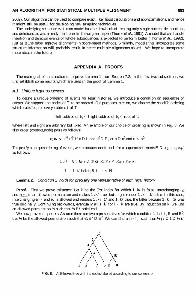
To de� ne a unique ordering of events for legal histories, we introduce a condition on sequences ofevents. We suppose the nodes of T to be ordered. For purposes later on, we choose the speci� c orderingwhich satis� es, for every subtree t of T ,

fleft subtree of tg < fright subtree of tg < root of t;

where left and right are arbitrary but � xed. An example of our choice of ordering is shown in Fig. 8. Wealso order (context,node) pairs as follows:

.c; n/ < .c0; n0/ if c D I and c0 D F , or c D c0 and n < n0:

To specify a unique ordering of events, we introduce condition 1 for a sequence of events E D .e1; : : : ; eN /

as follows:

1.i/ : ti \ tiC1 6D ? or .ci; ri/ < .ciC1; riC1/;

1 : 1.i/ holds; 8 1 · i < N:

Lemma 2. Condition 1 holds for precisely one representative of each legal history.

Proof. First we prove existence. Let k be the � rst index for which 1.k/ is false. Interchanging ek

and ekC1 is an allowed permutation and makes 1.k/ true, but might render 1.k ¡ 1/ false. In this case,interchanging ek¡1 and ek is allowed and renders 1.k ¡ 1/ and 1.k/ true, the latter because 1.k ¡ 1/ wastrue originally. Continuing backwards, eventually all 1.i/ for i · k are true. By induction on k, we � ndan allowed permutation ¼ such that ¼.E/ satis� es 1.

We now prove uniqueness. Assume there are two representatives for which condition 1 holds, E and E0.Let ¼ be the allowed permutation such that ¼.E/ D E0. We can � nd an i < j such that ¼.j/ C 1 D ¼.i/

FIG. 8. A 6-leaved tree with its nodes labeled according to our convention.

884 LUNTER ET AL.

(Christie, 1996). Since ¼ is an allowed permutation, ti \ tj D ?. E0 satis� es 1, therefore tj and ti are partof the left and right subtree of a node C0, respectively. Moreover, i C 1 6D j , because this would contradict1.i/ for E.

We prove by induction that for each k ¸ 0, a node Ck exists such that tj¡k is in the left subtree ofCk , ti is in the right subtree of Ck , and tj is contained in either. This means that there is no k such thati C 1 D j ¡ k; therefore, there is only one representative that satis� es the 1 condition.

We already proved that the induction hypothesis holds for k D 0. Assume it holds for certain k. Fourpossible cases are to be considered.

1. tj¡k¡1 \ ti 6D ? and tj¡k¡1 \ tj¡k 6D ?. This implies that Ck 2 tj¡k¡1 and hence tj¡k¡1 \ tj 6D ?.Since ¼ is an allowed permutation, ¼.i/ < ¼.j ¡ k ¡ 1/ and ¼.j ¡ k ¡ 1/ < ¼.j/, but this is impossible.

2. tj¡k¡1 \ ti 6D ? and tj¡k¡1 \ tj¡k D ?. This means that tj¡k¡1 is on the right subtree of Ck , andtherefore rj¡k¡1 > rj ¡ k, but this contradicts the 1 condition, since all cj D F because the history islegal.

3. tj¡k¡1 \ ti D ? and tj¡k¡1 \ tj¡k 6D ?. This means that tj¡k¡1 is on the left part of Ck . ForCkC1 D Ck , the condition of the induction holds.

4. tj¡k¡1 \ ti D ? and tj¡k¡1 \ tj¡k D ?. In this case, rj¡k¡1 < rj¡k < ri . The � rst inequality comesfrom the 1 condition, while the second one is from the induction hypothesis. However, these inequalitiesguarantee the existence of a proper CkC1.

In properly ordered sequences, legal sequences may be recognized by looking at pairs of events.

De� nition 2. A pair of events .e1; e2/ is called pairwise legal if t1 ¶ t2 ) l1.r2/ 6D ¡.

Lemma 3. The set

f.e1; : : : ; eN /j1 holds; .ei ; eiC1/ pairwise legal for i D 1; : : : ; N ¡ 1g

consists of precisely one representative of each legal history.

Proof. µ: Since 1 holds, at most one of each legal history is included. We prove that illegal historiesare not included. Let e1; : : : ; eN be an illegal sequence in the set. Let ei be the � rst event with ci D I ,that is, ri =2 Si . Since cj D F for j < i, in particular Si¡1 is legal. Suppose ti¡1 \ ti 6D ?. If ti¡1 ½ ti ,then ri =2 Si implies ri =2 Si¡1, but ri¡1 2 Si¡1 and ri¡1 is a descendant of ri , in contradiction with Si¡1

legal. So ti¡1 ¶ ti , but then ri =2 Si implies .ei¡1; ei/ is not pairwise legal. So ti¡1 \ ti D ?. Note thatci¡1 D F and ci D I , so 1 is false, which is the required contradiction.

¶: For all legal histories there exists a sequence obeying 1 by Lemma 2, and all neighboring pairs inlegal sequences are pairwise legal.

This result enables us to determine the sequences of events we want to sum over, by looking only atneighboring pairs. To use the inclusion/exclusion trick, we next have to characterize sequences of eventpairs that do not obey our condition.

A.2. Disallowed sequences and illegal sets

De� nition 3. Suppose Si is a legal state, and suppose that for all j D i; : : : ; k ¡ 1 we have .ej ; ejC1/

not pairwise legal or 1.j/ false. We call such (sub)sequences disallowed sequences.

Lemma 4. Let .ei ; eiC1; : : : ; ek/ be a disallowed sequence starting from state Si . Then:

(a) The sequence .cj ; rj /, i · j · k, is strictly decreasing.(b) All events ej with cj D F are disjoint.(c) For each node n, there is at most one event ej with n 2 tj and lj .n/ 6D ¡.

Note that statement (c) implies that there is at most one emission per leaf.


Proof. If .ej ; ejC1/ is not pairwise legal, then rjC1 is a descendant of rj and lj .rjC1/ D ¡. Thismeans that rj > rjC1 and cjC1 D I , so .cj ; rj / > .cjC1; rjC1/. If 1.j/ is false, then it directly followsfrom the de� nition of condition 1 that .cj ; rj / > .cjC1; rj C1/.

Now, that the sequence .cj ; rj / is strictly decreasing implies that, for some m, we have ci D ciC1 D¢ ¢ ¢ D cm D F and cmC1 D cmC2 D ¢ ¢ ¢ D ck D I . For i · j < m, the pair .ej ; ejC1/ is pairwise legalsince cjC1 D F ; therefore, we must have 1.j/ false, which implies that tj \ tjC1 D ?. Furthermore,tj \ tjC1 D ? and rj > rjC1 together imply that there exists a subtree t of T such that tj is in a rightsubtree of t , whereas tjC1 is in a left subtree of t . Applying this reasoning sequentially, we conclude thatfor all i · a < b · m there exists a subtree t such that ta (tb) is in a right (left) subtree of t . Hence,ta \ tb D ? and it follows that all of ti ; tiC1; : : : ; tm are pairwise disjoint.

Note that SmC1 is a legal state since Si is a legal state and all events ei ; eiC1; : : : ; em are legal events.For every m < j · k, that the event ej is illegal implies that rj =2 Sj . Now, suppose Sj \ tj 6D ?. Then,Sj must contain at least one descendant of rj , which is possible only if, since SmC1 is a legal state andrj =2 Sj , at least one of emC1; emC2; : : : ; ej¡1 has a birth at a descendant node of rj . But this contradictsthe fact that rmC1 > rmC2 > ¢ ¢ ¢ > rk , and therefore we must have Sj \ tj D ? for every m < j · k.

Finally, the results from the previous two paragraphs together imply (c).

Lemma 5. For a given legal initial state S, there is a one-to-one correspondence between illegal setsand disallowed sequences starting from S.

Proof. We prove the correspondence by establishing two injections.From disallowed sequence to illegal set: The events with cj D F are pairwise disjoint, and their trees

not the subtree of any other because the initial state is legal. The trees with cj D I may be subtreesof another tk , in which case lk.rj / D ¡, so the events form an illegal set. There is only one disallowedsequence giving rise to this set, since the sequence .cj ; rj / corresponding to the disallowed sequence isordered.

From illegal set to disallowed sequence: Take the events whose trees are not a subset of another andwhose root is in S, sorted decreasing by root. Follow them by the other events, sorted decreasing by root.A disallowed sequence results.

A.3. Proof of Lemma 1

For ease of reference, we here restate the lemma. We denote by E.K/ a set of legal sequences of eventswhich emit the pre� xes of the given sequences A1; : : : ; Ak up to position K D .K1; : : : ; Kk/ and whichcontains precisely one representative of each history. The quantity of interest is the likelihood

P .K/ :DX

.e1;:::;eN /2E.K/

p.e1/ ¢ ¢ ¢ p.eN /:

Lemma 1. The likelihood P .K/ satis� es the following equation:

P .K/ DX

e

P .K ¡ ve/p.e/

¡X

fe1;e2g illegal

P .K ¡ ve1 ¡ ve2 /p.e1/p.e2/

CX

fe1;e2;e3g illegal

P .K ¡ ve1 ¡ ve2 ¡ ve3/p.e1/p.e2/p.e3/

¡ ¢ ¢ ¢ :

Here, ve is the emission vector corresponding to the event e, that is, a k-dimensional vector whosecomponent corresponding to each leaf is 0 if the leaf is labeled ¡, or 1 otherwise.

886 LUNTER ET AL.

Proof. Let S.e/ denote the state after event e in state S. De� ne PS.K/ to be the likelihood of emittinglegal sequences up to position K and ending up in state S. We allow illegal states S, in which casePS.K/ D 0 always. For brevity, we denote by C.S0; e0; S1; e1; : : : ; en¡1; Sn/ the condition S0.e0/ DS1 ^ : : : ^ Sn¡1.en¡1/ D Sn, and by Dis.S; e0; : : : ; en/ the condition that .e0; : : : ; en/ is a disallowedsequence when starting from state S. Then

PS.K/ DX

.S 0;e/:C.S 0;e;S/

PS 0.K ¡ ve/p.e/

¡X

.S 0;e;S 00;e0/:C.S 00;e0;S0;e;S/^Dis.S 00;e0;e/

PS 00.K ¡ ve ¡ ve0/p.e0/p.e/

CX

.S 0;e;S00;e0;S 000;e00/:C.S 000;e00;S 00;e0;S0;e;S/^

^ Dis.S000;e00;e0;e/

PS000.K ¡ ve ¡ ve0 ¡ ve00/p.e00/p.e0/p.e/

¡ ¢ ¢ ¢ :

This recursion sums over all sequences of events which do not have disallowed subsequences, since allterms in the � rst line that include a disallowed subsequence (of length 2) are subtracted in the second line;this also subtracts terms involving disallowed subsequences of length 3 that were not included in the � rstplace, which are added in again in the third line, and so on. By Lemma 3, this implies that we indeedsum over all sequences of legal events (which end up in state S). Note that for illegal states S, PS.K/ D 0always, so we may de� ne Dis.S; e0; : : : / arbitrarily for illegal states S.

Now we sum the recursion equation over all states S. The left-hand side becomes P .K/. The � rstsummation on the right-hand side turns into

X

S

X

.S 0;e/:S 0.e/DS

PS 0.K ¡ ve/p.e/ DX

.S 0;e/

PS0.K ¡ ve/p.e/ DX

e

P .K ¡ ve/p.e/;

which is the desired term. Similarly, the second summation becomes

X

.S 00;e0;e/:Dis.S 00;e0;e/

PS 00.K ¡ ve ¡ ve0/p.e0/p.e/:

Observe that the summand is independent of the ordering of events e0; e. Hence, we can also sum overillegal sets of events and over S 00, using Lemma 5. This turns the summation into

X

S 00

X

fe0;eg illegal

PS 00.K ¡ ve ¡ ve0/p.e0/p.e/ DX

fe0;eg illegal

P .K ¡ ve ¡ ve0/p.e0/p.e/;

which is the desired term. All other summations are dealt with analogously. Note that only � nitely manysummands contribute to the recursion, since illegal sets have a bounded number of elements.

APPENDIX B. STATES FOR THE HJP RECURSION

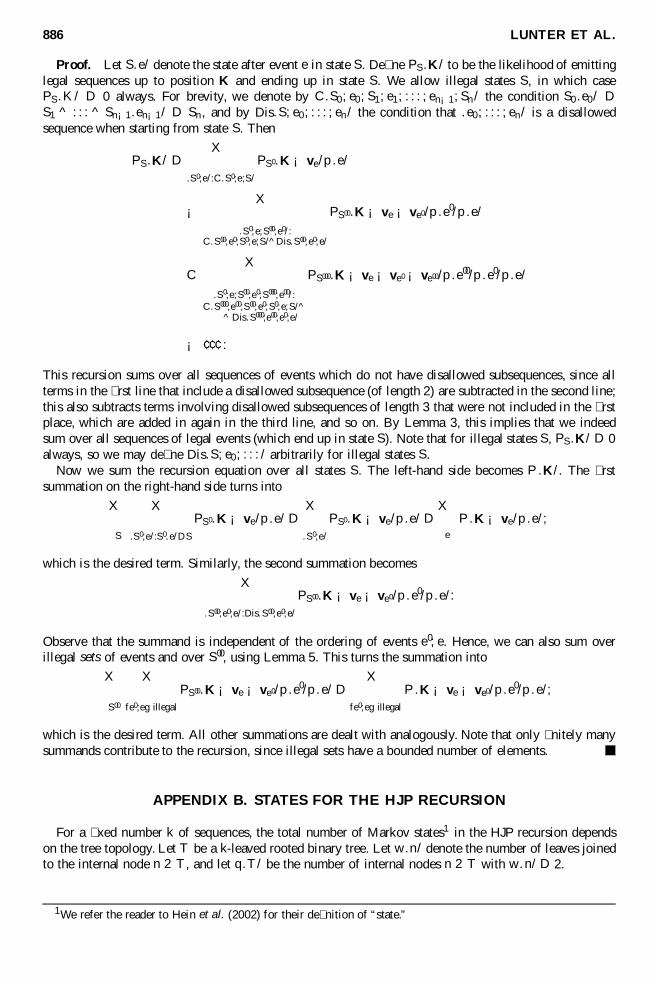
For a � xed number k of sequences, the total number of Markov states1 in the HJP recursion dependson the tree topology. Let T be a k-leaved rooted binary tree. Let w.n/ denote the number of leaves joinedto the internal node n 2 T , and let q.T / be the number of internal nodes n 2 T with w.n/ D 2.

1We refer the reader to Hein et al. (2002) for their de� nition of “state.”


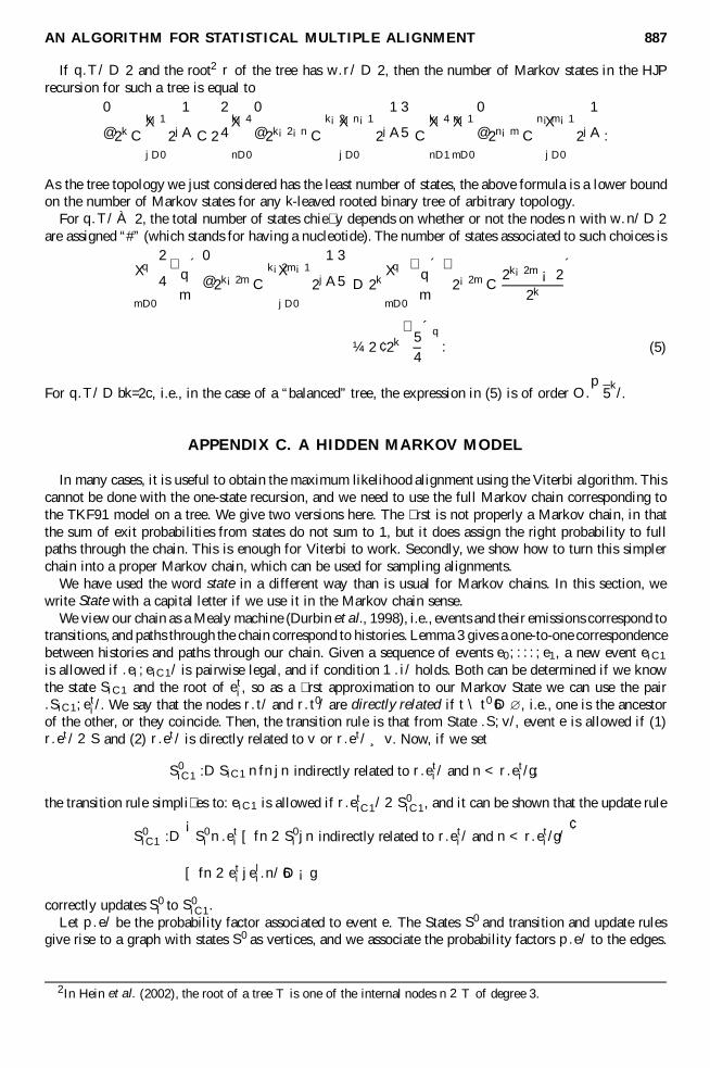
If q.T / D 2 and the root2 r of the tree has w.r/ D 2, then the number of Markov states in the HJPrecursion for such a tree is equal to

0

@2k Ck¡1X

jD0

2j

1

A C 2

2

4k¡4X

nD0

0

@2k¡2¡n Ck¡2¡n¡1X

jD0

2j

1

A

3

5 Ck¡4X

nD1

n¡1X

mD0

0

@2n¡m Cn¡m¡1X

jD0

2j

1

A :

As the tree topology we just considered has the least number of states, the above formula is a lower boundon the number of Markov states for any k-leaved rooted binary tree of arbitrary topology.

For q.T / À 2, the total number of states chie� y depends on whether or not the nodes n with w.n/ D 2are assigned “#” (which stands for having a nucleotide). The number of states associated to such choices is

qX

mD0

2

4³

q

m

´ 0

@2k¡2m Ck¡2m¡1X

jD0

2j

1

A

3

5 D 2k

qX

mD0

³q

m

´ ³2¡2m C 2k¡2m ¡ 2

2k

´

¼ 2 ¢ 2k

³54

´q

: (5)

For q.T / D bk=2c, i.e., in the case of a “balanced” tree, the expression in (5) is of order O.p

5k/.

APPENDIX C. A HIDDEN MARKOV MODEL

In many cases, it is useful to obtain the maximum likelihood alignment using the Viterbi algorithm. Thiscannot be done with the one-state recursion, and we need to use the full Markov chain corresponding tothe TKF91 model on a tree. We give two versions here. The � rst is not properly a Markov chain, in thatthe sum of exit probabilities from states do not sum to 1, but it does assign the right probability to fullpaths through the chain. This is enough for Viterbi to work. Secondly, we show how to turn this simplerchain into a proper Markov chain, which can be used for sampling alignments.

We have used the word state in a different way than is usual for Markov chains. In this section, wewrite State with a capital letter if we use it in the Markov chain sense.

We view our chain as a Mealy machine (Durbin et al., 1998), i.e., events and their emissions correspond totransitions, and paths through the chain correspond to histories. Lemma 3 gives a one-to-one correspondencebetween histories and paths through our chain. Given a sequence of events e0; : : : ; e1, a new event eiC1

is allowed if .ei ; eiC1/ is pairwise legal, and if condition 1.i/ holds. Both can be determined if we knowthe state SiC1 and the root of et

i , so as a � rst approximation to our Markov State we can use the pair.SiC1; et

i/. We say that the nodes r.t/ and r.t 0/ are directly related if t \ t 0 6D ?, i.e., one is the ancestorof the other, or they coincide. Then, the transition rule is that from State .S; v/, event e is allowed if (1)r.et / 2 S and (2) r.et / is directly related to v or r.et/ ¸ v. Now, if we set

S 0iC1 :D SiC1 n fn j n indirectly related to r.et

i/ and n < r.eti/g;

the transition rule simpli� es to: eiC1 is allowed if r.etiC1/ 2 S 0

iC1, and it can be shown that the update rule

S 0iC1 :D

¡S 0

i n .eti [ fn 2 S0

i j n indirectly related to r.eti/ and n < r.et

i/g/¢

[ fn 2 eti j el

i.n/ 6D ¡g

correctly updates S 0i to S 0

iC1.Let p.e/ be the probability factor associated to event e. The States S0 and transition and update rules

give rise to a graph with states S 0 as vertices, and we associate the probability factors p.e/ to the edges.

2In Hein et al. (2002), the root of a tree T is one of the internal nodes n 2 T of degree 3.

888 LUNTER ET AL.

To complete the graph, we introduce the initial and end States A and Ä. Furthermore, we introduce asingle edge (with p D

Qn2T In) between A and the State T and join each State except A to Ä by a single

edge (with p D 1). In this way, the product of probability factors along any path from A to Ä is just theprobability of the associated sequence of events, or history, under the TKF91 model. Since by our choiceof States, each permissible history is counted exactly once, the probabilities sum up to 1.

For sampling, it is necessary to have a proper Markov chain, i.e., have the probabilities of outgoingedges sum to 1, and the graph just de� ned can be turned into one by a scalar base change. Let PS bethe probability of being in State S, i.e., the sum of probabilities of all paths ending in S. Then, the stateequation can be written as PS D

PS 0 PS 0 tS 0S , where tS 0S is the transition matrix. If we introduce new

variables OPS D fSPS , then we can write OPS DP

S 0 OPS 0 OtS 0S , where OtS 0S D tS 0SfS=fS 0 . The graph becomes

a Markov chain ifP

SOtS0S D 1. A tedious but straightforward calculation shows that fS D

¡Qn2S In

¢¡1

solves this equation, and the transition probabilities become

Sie¡! SiC1 :

fSiC1

fSi

p.e/;

where fA D fÄ D 1.

ACKNOWLEDGMENTS

The authors wish to thank Rune Lyngsø and Alexei Drummond for helpful discussions and the refereesfor their thorough reading and detailed comments. Just before publication, Jens Ledet Jensen sent us analternative proof of the results presented here.3 This research is supported by EPSRC under grant HAMJWand by MRC under grant HAMKA. Y.S. Song is supported in part by a grant from the Danish NaturalScience Foundation (SNF-5503-13370).

REFERENCES

Christie, D.A. 1996. Sorting permutations by block-interchanges. Inf. Proc. Letters 60, 165–169.Durbin, R., Eddy, S., Krogh, A., and Mitchison, G. 1998. Biological Sequence Analysis, Cambridge University Press.Eddy, S. 2001. HMMER: Pro� le hidden markov models for biological sequence analysis (hmmer.wustl.edu/).Felsenstein, J. 1981. Evolutionary trees from DNA sequences: A maximum likelihood approach. J. Mol. Evol. 17,

368–376.Felsenstein, J. 2001. Phylip: Phylogeny Inference Package, University of Washington.Goldman, N. 1998. Effects of sequence alignment procedures on estimates of phylogeny. BioEssays 20, 287–290.Hein, J. 2001. An algorithm for statistical alignment of sequences related by a binary tree. Pac. Symp. Biocomp.,

179–190.Hein, J., Jensen, J.L., and Pedersen, C.N.S. 2002. Recursions for statistical multiple alignment. Technical Report 425,

Dept. of Theor. Stat., Univ. of Aarhus.Hein, J., Wiuf, C., Knudsen, B., Møller, M.B., and Wibling, G. 2000. Statistical alignment: Computational properties,

homology testing and goodness-of-�t. J. Mol. Biol. 302, 265–279.Hirshberg, D.S. 1977. Algorithms for the longest common subsequence problem. J. ACM 24, 664–675.Holmes, I., and Bruno, W.J. 2001. Evolutionary HMMs: A Bayesian approach to multiple alignment. Bioinformatics

17(9), 803–820.Jensen, J.L., and Hein, J. 2002. Gibbs sampler for statistical multiple alignment. Technical Report 429, Dept. of Theor.

Stat., Univ. of Aarhus.Jukes, T.H., and Cantor, C.R. 1969. Mammalian Protein Metabolism, chapter Evolution of protein molecules, 21–132,

Academic Press.Lee, M.S.Y. 2001. Unalignable sequences and molecular evolution. Trends in Ecology and Evolution 16, 681–685.

3This proof has appeared in: Lunter, G.A., Miklos, I., Drummond, A.J., Jensen, J.L., Hein, J. 2003. BayesianPhylogenetic Inference under a Statistical Insertion-Deletion Model. In: Benson, G., and Page, R. (eds.), WABI 2003,LNBI 2812, 228–244. (Note added in proof.)


Miklós, I. 2002. An improved algorithm for statistical alignment of sequences related by a star tree. Bull. Math. Biol.64, 771–779.

Mitchison, G. 1999. A probabilistic treatment of phylogeny and sequence alignment. J. Mol. Evol. 49, 11–22.Needleman, S.B., and Wunsch, C.D. 1970. A general method applicable to the search for similarities in the amino

acid sequences in two proteins. J. Mol. Biol. 48, 443–453.Sankoff, D., and Kruskall, J.B. 1983. Time Warps, String Edits and Macromolecules: The Theory and Practice of

Sequence Comparison, Addison-Wesley, Reading, PA.Steel, M., and Hein, J. 2001. Applying the Thorne–Kishino–Felsenstein model to sequence evolution on a star-shaped

tree. Appl. Math. Let. 14, 679–684.Thorne, J.L., Kishino, H., and Felsenstein, J. 1991. An evolutionary model for maximum likelihood alignment of DNA

sequences. J. Mol. Evol. 33, 114–124.Thorne, J.L., Kishino, H., and Felsenstein, J. 1992. Inching toward reality: An improved likelihood model of sequence

evolution. J. Mol Evol. 34, 3–16.Whelan, S., Lió, P., and Goldman, N. 2001. Molecular phylogenetics: State-of-the-art methods for looking into the

past. Trends Genet. 17, 262–272.

Address correspondence to:G.A. Lunter

Department of StatisticsUniversity of Oxford

Oxford, OX1 3TG, UK

E-mail: [email protected]

An Efficient Algorithm for Statistical Multiple Alignment on Arbitrary Phylogenetic Trees

Documents