An efficient 1D O CCAM’S inversion algorithm using analytically computed first- and second-order derivatives for dc resistivity soundings

ARTICLE IN PRESS

0098-3004/$ - se

doi:10.1016/j.ca

$Code on serv�Correspond

fax: +9140 234

E-mail addr1CSIR-TWA

Computers & Geosciences 31 (2005) 319–328

www.elsevier.com/locate/cageo

An efficient 1D OCCAM’S inversion algorithm usinganalytically computed first- and second-order derivatives

for DC resistivity soundings$

Nimisha Vedanti, Ravi P. Srivastava, John Sagode1, V.P. Dimri�

National Geophysical Research Institute, Council of Scientific and Industrial Research, Post Bag No. 724, Uppal Road,

Hyderabad 500 007, India

Abstract

An efficient algorithm has been developed for 1D resistivity inversion problem using both first- and second-order

derivatives, which are computed analytically. The second-order derivative matrix, which is not used in the OCCAM’s

inversion, has been incorporated into the algorithm employing analytical expressions. Computation of complicated

second-order derivatives in each iteration is circumvented by a new algorithm. These modifications result in stable

convergence of the OCCAM’s inversion and in general, better misfit can be achieved specially for smoothing parameter,

mo1: The modified inversion algorithm, coded in MATLAB was tested using two synthetic Schlumberger resistivity

sounding examples. Its application has been illustrated with field data from south India.

r 2004 Elsevier Ltd. All rights reserved.

Keywords: Hessian matrix; Jacobian matrix; Schlumberger sounding; Newton’s method; Smoothing parameter

1. Introduction

The OCCAM’s inversion algorithm was first intro-

duced by Constable et al. (1987) to find the smoothest

model that fits the magnetotelluric (MT) and Schlum-

berger geoelectric sounding data. The method gained

popularity in inversion studies and was applied to many

investigations (LaBrecque et al., 1996; Siripunvaraporn

and Egbert, 1996; Qian et al., 1997). In this scheme a

highly nonlinear problem is formulated in a linear

fashion, which obviates the computation of second-

e front matter r 2004 Elsevier Ltd. All rights reserve

geo.2004.10.015

er at http://www.iamg.org/CGEditor/index.htm.

ing author. Tel.: +9140 234 34 600;

34651.

ess: [email protected] (V.P. Dimri).

S Fellow.

order derivatives that carry useful curvature information

of the objective function.

In this paper the 1D OCCAM’s algorithm has been

improved by inclusion of second-order derivative matrix

known as Hessian that is computed analytically. This

leads to a quadratic equation approximation of the

objective function. The modified algorithm has been

tested on synthetic and real field resistivity sounding

data. It is found that the modified algorithm is more

stable and convergent than OCCAM’s inversion.

The computation of second-order derivatives in

Schlumberger resistivity sounding involves cumbersome

piece of algebra and therefore these derivatives are

computed numerically using finite difference schemes.

This introduces many unacceptable errors and requires

more computational time, which results in inaccurate

curvature information that decides the step of descent

where as computation of the derivatives analytically

d.

www.elsevier.com/locate/cageo

http://www.iamg.org/CGEditor/index.htm

ARTICLE IN PRESSN. Vedanti et al. / Computers & Geosciences 31 (2005) 319–328320

solves the problem. The analytic approach based on

recursive formulation provides faster computation of the

derivatives.

2. Formulation of the problem

The nonlinear resistivity inversion relates observed

data and model parameters by equation

Y ¼ gðxÞ þ n; (1)

where Y ¼ ðy1; . . . ; yN ; Þ is a vector representing ob-

servations at different half-electrode separations in

Schlumberger sounding, N is number of half-electrode

separations, gðxÞ ¼ ðg1ðxÞ; . . . ; gN ðxÞÞ represents pre-

dicted data at different half-electrode separations, and

n is the measurement noise.

Various schemes to treat this non-linear problem are

described in detail by Dimri (1992). Terminology used

here closely follows Chernoguz (1995) with some

differences arising due to Constable et al. (1987).

Following Constable et al. (1987) the inverse problem

is posed as a constrained optimization problem, set forth

to minimize misfit X ¼ jjWY� WgðxÞjj; subject to the

constraint that roughness R ¼ jj@xjj is also minimized.

This can be converted to an unconstrained problem by

the use of Lagrange parameter m as follows:

U ¼1

2jj@xjj2 þ

1

2mfðW DYðxÞÞTðW DYðxÞ � w2�Þg; (2)

where @ is N N matrix defined by Constable et al.

(1987) as

@ ¼

0 0 ::: ::: 0

�1 1 ::: ::: 0

0 �1 1 ::: 0

: : : : :

: : : : :

0 0 ::: �1 1

0BBBBBBBB@

1CCCCCCCCA:

W is weighting matrix, w� is acceptable misfit value and,m is a Lagrange parameter used to optimize the

constrained functional ‘U’ (Smith, 1974) and DYðxÞ ¼

WY� WgðxÞ: If we expand the functional in Taylor’s

series at x ¼ xk (say) we get

Uðxk þ d; m;YÞ ¼ Uðxk; m;YÞ þ JTk dþ

1

2dTQkd;

where

Jk ¼ rxU ¼ @T@x �1

mðWGðxÞÞTW DYðxÞ

and

Qk ¼ r2xU ¼ @T@�1

mrxfðWGðxÞÞTW DYðxÞg:

Using the identity

rxfWGðxÞÞTW DYðxÞg ¼ ðWHðxÞÞTW DYðxÞ

� ðWGðxÞÞTWGðxÞ

the Qk becomes

Qk ¼ r2xU

¼ @T@�1

mfðWGðxÞÞTWGðxÞ

� ðWHðxÞÞTW DYðxÞg

where GðxÞ is Jacobian of gðxÞ and HðxÞ is Hessian of

gðxÞ:If we define

ðWHÞTW DY ¼

Xj

WHjW DYj as q;

where in Hj is Hessian of gðxÞ evaluated at jth data point

and DYj ¼ yj � gjðxÞ; q is the nonlinear part of the

Hessian, then minimization of the functional (2) using

Newton’s method for ith iteration step di yields

di ¼ � @T@þ m�1fWGðxÞTWGðxÞ � qg� �1

@T@x � m�1WGðxÞTW DYðxÞ�

x¼xi: ð3Þ

Thus xiþ1 ¼ xi þ di forms the iterative basis for the

optimization of functional (2). Eq. (3) gives generalized

OCCAM’s correction steps. By setting q as a null

matrix, the equation gives the model correction of the

popular OCCAM’s inversion algorithm. The OCCAM’s

optimization in Eq. (3) can be viewed as two sub-

algorithms, where primary optimizes the functional U

for different values of x and m and secondary optimizes

only misfit function. The difficulty may arise when the

primary suggests corrections in the direction of decreas-

ing U and secondary moves in search of decreasing

misfit without regarding the roughness. Thus due to lack

of curvature information in the OCCAM’s inversion,

secondary algorithm becomes blind in the direction of

true minimum of w2; when the requirement of the

primary algorithm to reduce U is overpowering.

Another problem in OCCAM’s inversion is the choice

of Lagrange’s parameter m. If we take mo1 for

minimization of functional used in standard OCCAM’s

inversion, the algorithm tends to be blind to minimize

misfit function in the absence of the curvature informa-

tion. Hence, there is need to incorporate curvature

information in terms of Hessian matrix. If we take mp1

in Eq. (3) the nonlinear part carrying curvature

information, will contribute to the convergence. In our

work we include the curvature information in the

OCCAM’s model correction steps. From Newton–-

Gauss method we have,

xiþ1 ¼ xi þ aidi; (4)

ARTICLE IN PRESSN. Vedanti et al. / Computers & Geosciences 31 (2005) 319–328 321

where ai is the extra smoothing parameter which

uses curvature information as provided by Hessian

terms.

Following Chernoguz (1995) we have

ai ¼�j0ð0Þj00ð0Þ if 0oaip1;

1 otherwise;

((5)

where j0ð0Þ is the first-order derivative and j00ð0Þ is the

second-order derivative of Uðxi þ aidi; m;YÞ that are

computed as

j0ð0Þ ¼ dTi ½@@xi � m�1WGðxiÞTW DYðxiÞ�

and

j00ð0Þ ¼ � dTi ½@@xi � m�1fWGðxiÞTW DYðxiÞ

� WHðxiÞTW DYðxiÞdig�;

where the computation of Hessian matrix is involved in

each iteration.

Generally, derivatives are calculated using finite-

difference techniques. The two most commonly used

techniques are forward difference, which is accurate to

first order and central difference, which is accurate to

second order. In general, errors in forward difference

approximation become unacceptably large during the

last few iterations and often in such cases, central

difference scheme is used. Computation of partial

derivatives using central difference requires twice

evaluations of forward functional than forward

difference (Constable et al., 1987), and takes more

computational time. Hence it is not worthwhile to

use central difference for computation of Jacobian

and Hessian matrices. Errors associated with computa-

tion of Hessian terms have a substantial effect on

inversion algorithm. The use of analytical expre-

ssions instead of finite difference solves all the above

problems.

In OCCAM’s inversion Constable et al. (1987) have

computed Jacobian matrix for Schlumberger sounding

using analytical expressions and have concluded that the

Schlumberger resistivity inversion with finite-difference

derivatives takes 15 times more computational time than

the analytical derivatives. Hence in our algorithm, the

Hessian terms are calculated analytically.

For very large data sets computation of the Hessian in

each iteration becomes very tedious and time consum-

ing, hence we follow Chernoguz (1995) to minimize the

computations and at the same time to preserve the

curvature information using Hessian matrix in the extra

smoothing parameter a. In our algorithm Eq. (3) can be

used for first two iterations to get the two consecutive

values of a that are less than 1, and then the next

correction step can be deduced using a relation

ai ¼ 1� expð�tisÞ; (6)

where t and s are positive scalar constants (sX1) in ith

iteration, given as

t ¼ � ln ð1� a1Þ;

s ¼ log2½ln ð1� a2Þ= ln ð1� a1Þ�: ð7Þ

Eq. (5) is used to find the two consecutive values of a,i.e. a1 and a2 that are less than 1. In subsequent

iterations, Eq. (6) can be applied directly to find the

values of extra smoothing parameter to be used in

correction steps of Eq. (4). This avoids computation of

the tedious Hessian matrix in each iteration. In the

modified algorithm we choose initial model at random

as in the case of global optimization techniques. The

above-described inversion algorithm is coded in MA-

TLAB and can run on any machine. The weighting

matrix used in the code is taken as identity if uncertainty

in the data is not known. Step wise description of the

MATLAB code is given in Appendix A.

3. Analytical expressions of derivatives

The forward calculation for Schlumberger apparent

resistivity over a layered earth is given as

ra ¼AB

2

� �2 Z10

T1ðlÞJ1AB

2l

� �ldl; (8)

where J1 is the first-order Bessel’s function of the first

kind, AB/2 is the half-electrode spacing, l is electrode

parameter, T1 is the resistivity transform (Koefoed,

1976) that can be calculated recursively as

Ti�1 ¼Ti þ ri�1 tanhðlti�1Þ

1þ Ti tanhðlti�1Þ=ri�1

;

where ri and ti are the resistivity and thickness of ith

layer, respectively.

For the last layer TM ¼ rM ; where M is number of

layers.

Using fast Hankel transforms apparent resistivity can

be written as (Ghosh, 1971):

ra ¼X

K

T1ðlK Þf K ; (9)

where f K are the filter coefficients and K is the number

of coefficients.

3.1. First-order derivatives

The first-order derivatives of Eq. (9) are

qraqrj

¼X

K

qT1ðlK Þ

qrj

f K ; (10)

ARTICLE IN PRESS

Table 2

Synthetic data generated using input model given in (a) Table

1A and (b) Table 1B

AB/2 (m) Apparent

resistivity

(Om)

Log 10 apparent

resistivity

(Om)

(a)

2.50 8.69 0.94

3.00 9.05 0.96

3.70 9.71 0.99

4.60 10.79 1.03

5.80 12.61 1.10

7.20 15.26 1.18

8.40 17.95 1.25

10.00 22.08 1.34

12.50 29.67 1.47

16.00 42.05 1.62

20.00 57.78 1.76

25.00 78.35 1.89

30.00 98.68 1.99

37.00 125.21 2.10

46.00 154.72 2.19

58.00 185.90 2.27

72.00 212.54 2.33

84.00 229.22 2.36

100.00 245.38 2.39

125.00 261.82 2.42

160.00 275.04 2.44

200.00 283.37 2.45

250.00 289.15 2.46

N. Vedanti et al. / Computers & Geosciences 31 (2005) 319–328322

where

qT1

qrj

¼qT1

qT2

qT2

qT3� � �

qTj�1

qTj

qTj

qrj

; (10a)

qTj

qTjþ1¼ ½1� tanh2ðtjlK Þ�=Cj ; (10b)

qTj

qrj

¼ tanhðtjlK Þ½1þ T2jþ1=r

2j

þ 2Tjþ1 tanhðtjlK Þ=rj �=Cj ; ð10cÞ

and

Cj ¼ ½1þ tanh2ðtjlK ÞTjþ1=rj �2; (10d)

also

qTM

qrM

¼ 1; (11)

since TM ¼ rM for the last layer.

3.2. Second-order derivatives

The second-order derivatives of Eq. (9) are

qraqrjqri

¼X

K

q2T1ðlK Þ

qrjqri

f K : (12)

Table 1

Input synthetic models

Input model

(Om)

Input model

log10(resistivity)

(Om)

Inverted model

predicted log 10

(resistivity)

(Om)

Error (Om)

(a) Model 1a

8.10 0.91 0.90 1.02

15.40 1.19 1.31 0.76

166.40 2.22 1.91 2.04

215.50 2.33 2.32 1.02

300.40 2.48 2.48 1.00

(b) Model 2b

8.00 0.90 0.93 0.93

15.60 1.19 1.25 0.87

60.30 1.78 1.63 1.41

112.20 2.05 1.97 1.20

210.30 2.32 2.29 1.07

375.80 2.58 2.57 1.02

Error (Om) ¼ 10(log10(input model) �log10 (inverted model).aNo. of layers is 5 and thickness of each layer is 2.5m.bNo. of layers is 6 and thickness of each layer is 3.5m.

300.00 292.49 2.47

(b)

2.50 8.22 0.91

3.00 8.36 0.92

3.70 8.64 0.94

4.60 9.10 0.96

5.80 9.91 1.00

7.20 11.08 1.04

8.40 12.25 1.09

10.00 14.04 1.15

12.50 17.28 1.24

16.00 22.70 1.36

20.00 30.02 1.48

25.00 40.60 1.61

30.00 52.44 1.72

37.00 70.47 1.85

46.00 94.83 1.98

58.00 127.02 2.10

72.00 161.69 2.21

84.00 187.91 2.27

100.00 217.66 2.34

125.00 253.67 2.40

160.00 288.15 2.46

200.00 313.16 2.50

250.00 332.26 2.52

300.00 343.99 2.54

ARTICLE IN PRESS

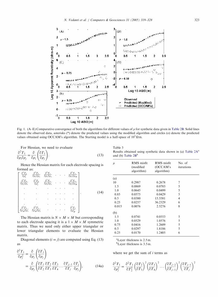
Fig. 1. (A–E) Comparative convergence of both the algorithms for different values of m for synthetic data given in Table 2B. Solid linesdenote the observed data, asterisks (*) denote the predicted values using the modified algorithm and circles (o) denote the predicted

values obtained using OCCAM’s algorithm. The Starting model is a half-space of 105Om.

Table 3

Results obtained using synthetic data shown in (a) Table 2Aa

and (b) Table 2Bb

m RMS misfit

(modified

algorithm)

RMS misfit

(OCCAM’s

algorithm)

No. of

iterations

(a)

10 0.2987 0.2678 7

1.5 0.0869 0.0703 5

1.0 0.0645 0.0499 5

0.85 0.0575 0.0429 5

0.5 0.0380 15.5581 4

0.25 0.0257 36.2329 6

0.015 0.0076 2.5276 8

(b)

1.5 0.0741 0.0553 5

1.0 0.0529 1.0576 5

0.75 0.0416 1.2609 5

0.5 0.0297 1.8186 5

0.25 0.0170 1.2405 6

aLayer thickness is 2.5m.bLayer thickness is 3.5m.

N. Vedanti et al. / Computers & Geosciences 31 (2005) 319–328 323

For Hessian, we need to evaluate

q2T1

qriqrj

¼qqri

qT1

qrj

!: (13)

Hence the Hessian matrix for each electrode spacing is

formed as:q2T1

qr21

q2T1

qr1qr2q2T1

qr1qr3: : : q2T1

qr1qrM

q2T1

qr2@r1q2T1

qr22

q2T1

qr2qr3: : : q2T1

qr2qrM

: : : : : : :

: : : : : : :

: : : : : : :

: : : : : : :q2T1

qrMqr1q2T1

qrMqr2: : : : q2T1

qr2M

266666666666664

377777777777775: (14)

The Hessian matrix is N M M but corresponding

to each electrode spacing it is a 1 M M symmetric

matrix. Thus we need only either upper triangular or

lower triangular elements to evaluate the Hessian

matrix.

Diagonal elements (i ¼ j) are computed using Eq. (13)

as

q2T1

qr2j¼

qqrj

qT1

qrj

!

¼qqrj

qT1

qT2

qT2

qT3

qT3

qT4. . .

qTj�1

qTj

qTj

qrj

!; ð14aÞ

where we get the sum of i terms as

q2T1

qr2j¼

q2T1

qT22

qT2

qT3

� �2 qT3

qT4

� �2

. . .qTj�2

qTj�1

� �2 qTj�1

qTj

� �2

ARTICLE IN PRESS

1 2 3 4 5 60

3.5

3

2.5

2

1.5

1

0.5

= 1.5

1.0

0.75

0.50

0.25

=

=

=

=

50

100

150

200

250

(A)

RM

S m

isfit

RM

S m

isfit

No. of Iterations

µ

µ= 1.50

1.00

0.75

0.50

0.25

=

=

=

=


qTj

qrj

!2

þqT1

qT2

q2T2

qT23

!qT3

qT4

� �2

. . .qTj�2

qTj�1

� �2

qTj�1

qTj

� �2 qTj

qrj

!2

þ . . .þqT1

qT2

qT2

qT3. . .

q2Tk

qT2kþ1

qTkþ1

qTkþ2

� �2

. . .qTj�1

qTj

� �2

þ . . .þqT1

qT2

qT2

qT3

qT3

qT4. . .

qTj�2

qTj�1

qTj�1

qTj

q2Tj

qr2jð14bÞ

and nondiagonal elements are represented as

q2T1

qriqrj

¼q2T1

qT22

qT2

qT3

� �2 qT3

qT4

� �2

. . .qTi

qTj

qTi

qri

qTj

qrj

þqT1

qT2

q2T2

qT23

!qT3

qT4

� �2 qT4

qT5. . .

qTi

qri

qTj

qrj

þqT1

qT2

qT2

qT3

q2T3

qT24

. . .qTi

qTj

qTi

qri

qTj

qrj

þ . . .

þqT1

qT2

qT2

qT3

qT3

qT4. . .

qTi�1

qTi

qTj

qrj

qqri

qTi

qTj

� �;

ð14cÞ

where in

qqrj

qTj

qTjþ1

� �¼

qqTjþ1

qTj

qrj

!(14d)

¼ 2 tanhðtjlK ÞTjþ1½1

þ Tjþ1 tanhðtjlK Þ=rj �qTj

qTjþ1

� ��r2j Cj ð14eÞ

q2Tj

qr2j¼ � 2 tanhðtjlkÞf1� tanh2ðtjlkÞgT

2jþ1=frj

þ tanhðtjlkÞTjþ1g3; ð14fÞ

q2Tj

qT2jþ1

¼ � 2r2j tanhðtjlK Þ½1

� tanh2ðtjlkÞ�=frj þ tan hðtjlkÞTjþ1g; ð14gÞ

Cj is the same as in Jacobian computations. It is

advantageous to compute all the terms of the Hessian

and the adjoining products simultaneously to save

computational time and memory.

1 2 3 4 5 60

(B) No. of Iterations

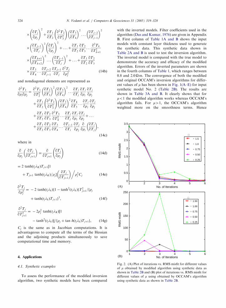
Fig. 2. (A) Plot of iterations vs. RMS misfit for different values

of m obtained by modified algorithm using synthetic data as

shown in Table 2B and (B) plot of iterations vs. RMS misfit for

different values of m using obtained by OCCAM’s algorithm

using synthetic data as shown in Table 2B.

4. Applications

4.1. Synthetic examples

To assess the performance of the modified inversion

algorithm, two synthetic models have been compared

with the inverted models. Filter coefficients used in the

algorithm (Das and Kumar, 1976) are given in Appendix

B. First column of Table 1A and B shows the input

models with constant layer thickness used to generate

the synthetic data. This synthetic data shown in

Table 2A and B is used to test the inversion algorithm.

The inverted model is compared with the true model to

demonstrate the accuracy and efficacy of the modified

algorithm. Errors of the inverted parameters are shown

in the fourth columns of Table 1, which ranges between

0.8 and 2.0Om. The convergence of both the modified

and original OCCAM’s inversion algorithms for differ-

ent values of m has been shown in Fig. 1(A–E) for input

synthetic model No. 2 (Table 2B). The results are

shown in Table 3A and B. It clearly shows that for

mo1 the modified algorithm works whereas OCCAM’s

algorithm fails. For m41; the OCCAM’s algorithm

weighted more on the smoothness terms. Hence

ARTICLE IN PRESS

2

2.5

= 1.00

µ

N. Vedanti et al. / Computers & Geosciences 31 (2005) 319–328 325

the modified algorithm can be seen as generalized

OCCAM’s inversion.

It is worth pointing here that smaller values of mshould be preferred to give less weight to the smooth-

ness/roughness part as described in Eq. (2). The bias

of algorithm to generate smooth models should be

avoided whenever it is not required. Variation of

RMS misfit with iteration number has been shown in

Fig. 2 for different values of m: The modified algorithm

shows stable convergence, while erratic variation in

RMS misfit of OCCAM’s algorithm has been observed

for mo1: We observed a remarkable difference in

convergence between modified inversion algorithm

and existing OCCAM’s algorithm for mo1: Results

obtained using two different filters is shown in

Appendix C.

RM

S m

isfit

1 2 3 4 5 60

0.5

1

1.5

= 0.10 = 0.05 = 0.0125 = 0.005

No. of Iterations

Fig. 4. Plot of iterations vs. RMS misfit for different values of musing field data of SGT.

4.2. Field example

The developed algorithm is used to invert 1D

Schlumberger resistivity sounding data. The data from

Southern Granulitic Terrain (SGT) of India

(1113405400N, 781301800E) over a 10 km long profile is

given in Appendix D. This data has been collected

by Deep Resistivity Sounding (DRS) Group of

NGRI, Hyderabad, India using the Scintrex make Deep

Resistivity Equipment, TSQ4-10 KVA. The convergence

of the modified algorithm has been shown in

Fig. 3(A–F). We have assumed starting model as a

Iteration No. 1 Iteratio

Iteration No. 4 Iteratio

8

6

4

3

2

2

5

4

3

2

10

02

0 2 4 0

0 2 4

4

(A) (B)

(D) (E)

ObservedPredicted

3.5

2.5

1.5

3

2

4

3.5

2.5

1.5

log 10(AB/2) [m] log 10(ALog1

0 [A

ppar

ent R

esis

tivity

] [oh

m-m

]Lo

g10

[App

aren

t Res

istiv

ity] [

ohm

-m]

Fig. 3. (A–F) Convergence of modified algorithm for m ¼ 0:0125 usinobserved data, asterisks (*) denote predicted values using modified al

half-space of 105Om, which was far from the observed

one. The modified algorithm searches for the lowest

misfit until it becomes constant with further iterations as

shown in Fig. 4. This is the global optimization strategy

of our inversion scheme, where the existing OCCAM’s

inversion fails for mo1: Results obtained using the

modified algorithm for different values of m, are shownin Table 4.

n No. 2

n No. 5 Iteration No. 6

Iteration No. 3

4

3

2

4 0 2 4

2 4 0 2 4

(C)

(F)

4.5

3.5

2.5

1.5

1.5

3

2

4

3.5

2.5

B/2) [m] log 10(AB/2) [m]

g field data of SGT as given in Appendix D. Solid lines denote

gorithm. The starting model is a half-space of 105Om.

ARTICLE IN PRESS

Table 4

Results obtained by modified algorithm using field data over SGT

Iteration No. RMS misfit

m ¼ 1:0 m ¼ 0:1 m ¼ 0:05 m ¼ 0:0125 m ¼ 0:005

1 2.3147 2.3147 2.3147 2.3147 2.3147

2 1.9339 2.3385 2.4075 2.4804 2.4967

3 0.493 0.1925 0.1703 0.2209 0.3221

4 0.1751 0.0977 0.0851 0.0777 0.0986

5 0.1682 0.0952 0.0795 0.0593 0.0529

6 0.168 0.0951 0.0792 0.0584 0.0494


5. Concluding remarks

The modified OCCAM’s inversion algorithm is very

efficient, robust and simple to be used for 1D resistivity

inversion. The modified algorithm finds an alternate way

to simplify the nonlinear resistivity inversion problem

without linearizing it. The code computes the first- and

second-order derivatives of Schlumberger resistivity

analytically and in general the convergence is obtained

within 5–6 iterations. We have demonstrated the efficacy

of the algorithm with two synthetic examples. For mo1;the modified gives less RMS error than OCCAM’s with

equal number of iterations. For m41 our modified

algorithm yields similar results as OCCAM’s. Hence our

inversion algorithm may be considered as generalized

OCCAM’s inversion.

Acknowledgements

Authors express heartfelt thanks towards late Profes-

sor P.S. Moharir for his invaluable suggestions to

develop the MATLAB codes. We are thankful to

Professor Peter Weidelt and reviewers of the manuscript

for many constructive comments that helped us in

improving quality of the work. We acknowledge Dr.

S.B. Singh, Head, Deep Resistivity Sounding Group,

NGRI Hyderabad for providing DC geoelectric sound-

ing data of SGT. One of the authors John Sagode

acknowledges CSIR, India and TWAS, Italy for the

award of fellowship.

Appendix A. Stepwise code description of 1D nonlinear

resistivity inversion algorithm

1.
Input to the program:
(a) digital resistivity filters (as per the choice of

user);

(b) AB/2 vs. apparent resistivity (in log10);

(c) starting model.

2.

Predicted apparent resistivity values corresponding

to each AB/2 are computed using starting model by

the forward algorithm.

3.
First-order and second-order derivatives are com-
puted analytically which is multiplied with the

filter coefficients to obtain apparent resistivity

values.

4.
First-order derivatives are arranged to form Jaco-
bian and second-order derivative are arranged to

form Hessian matrix.

5.
Predicted resistivity values are matched with the
observed data, and the difference is computed.

6.
With the above-mentioned steps the functional to be
minimized is ready.

7.
Search for m that minimizes the objective functional
depending upon user’s choice (Golden section

search may be used for this purpose).

8.
Iteration steps are computed using Eq. (4) and
values of a are computed using Eq. (5).

9.
If in any two consecutive iteration different values of
a are obtained such that these are o1, then Hessian

computation is bypassed and the value of a obtainedby consecutive a values are used in iteration steps,

otherwise a ¼ 1:
10. Above procedure is repeated until two consecutive
misfit values o1 having difference of o0.001 is

obtained.

Appendix B. Schlumberger coefficients as given by Das

and Kumar (1976) are

Sampling interval
ln 10/6
Shift
+0.1343155
Total number of filter points
14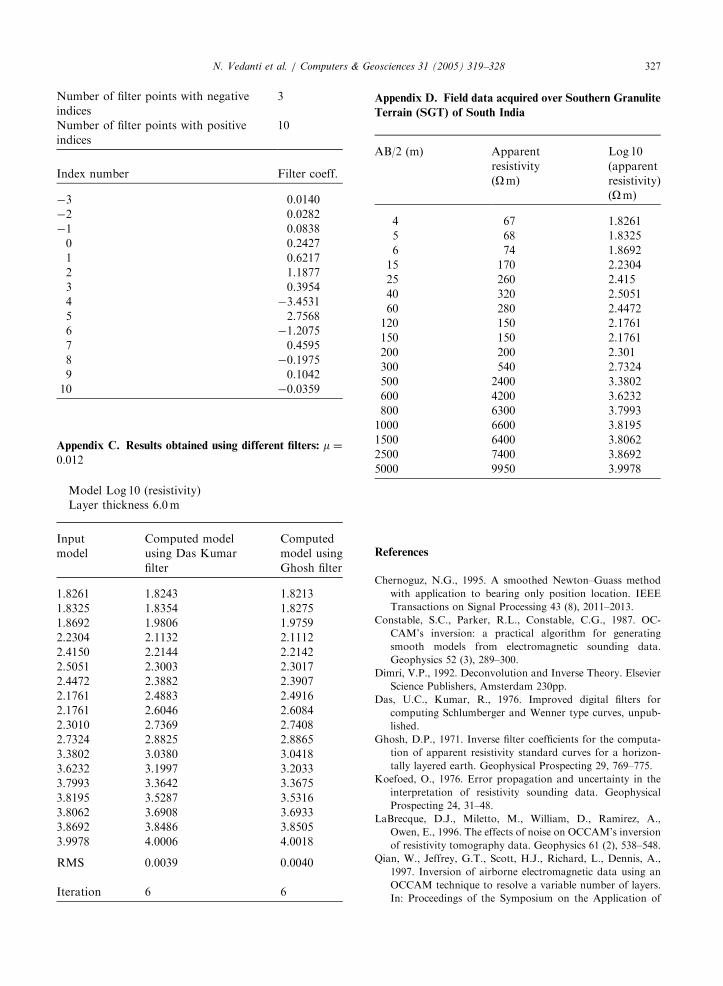

ARTICLE IN PRESSN. Vedanti et al. / Computers & Geosciences 31 (2005) 319–328 327

Number of filter points with negative

indices

3

Number of filter points with positive

indices

10

Index number
Filter coeff.
�3
0.0140
�2
0.0282
�1
0.0838
0
0.2427
1
0.6217
2
1.1877
3
0.3954
4
�3.4531
5
2.7568
6
�1.2075
7
0.4595
8
�0.1975
9
0.1042
10
�0.0359
Appendix C. Results obtained using different filters: m ¼

0:012

Model Log 10 (resistivity)

Layer thickness 6.0m

Input

model

Computed model

using Das Kumar

filter

Computed

model using

Ghosh filter

1.8261
1.8243 1.8213
1.8325
1.8354 1.8275
1.8692
1.9806 1.9759
2.2304
2.1132 2.1112
2.4150
2.2144 2.2142
2.5051
2.3003 2.3017
2.4472
2.3882 2.3907
2.1761
2.4883 2.4916
2.1761
2.6046 2.6084
2.3010
2.7369 2.7408
2.7324
2.8825 2.8865
3.3802
3.0380 3.0418
3.6232
3.1997 3.2033
3.7993
3.3642 3.3675
3.8195
3.5287 3.5316
3.8062
3.6908 3.6933
3.8692
3.8486 3.8505
3.9978
4.0006 4.0018
RMS
0.0039 0.0040
Iteration
6 6
Appendix D. Field data acquired over Southern Granulite

Terrain (SGT) of South India

AB/2 (m)
Apparent
resistivity

(Om)

Log 10

(apparent

resistivity)

(Om)

4
67 1.8261
5
68 1.8325
6
74 1.8692
15
170 2.2304
25
260 2.415
40
320 2.5051
60
280 2.4472
120
150 2.1761
150
150 2.1761
200
200 2.301
300
540 2.7324
500
2400 3.3802
600
4200 3.6232
800
6300 3.7993
1000
6600 3.8195
1500
6400 3.8062
2500
7400 3.8692
5000
9950 3.9978
References

Chernoguz, N.G., 1995. A smoothed Newton–Guass method

with application to bearing only position location. IEEE

Transactions on Signal Processing 43 (8), 2011–2013.

Constable, S.C., Parker, R.L., Constable, C.G., 1987. OC-

CAM’s inversion: a practical algorithm for generating

smooth models from electromagnetic sounding data.

Geophysics 52 (3), 289–300.

Dimri, V.P., 1992. Deconvolution and Inverse Theory. Elsevier

Science Publishers, Amsterdam 230pp.

Das, U.C., Kumar, R., 1976. Improved digital filters for

computing Schlumberger and Wenner type curves, unpub-

lished.

Ghosh, D.P., 1971. Inverse filter coefficients for the computa-

tion of apparent resistivity standard curves for a horizon-

tally layered earth. Geophysical Prospecting 29, 769–775.

Koefoed, O., 1976. Error propagation and uncertainty in the

interpretation of resistivity sounding data. Geophysical

Prospecting 24, 31–48.

LaBrecque, D.J., Miletto, M., William, D., Ramirez, A.,

Owen, E., 1996. The effects of noise on OCCAM’s inversion

of resistivity tomography data. Geophysics 61 (2), 538–548.

Qian, W., Jeffrey, G.T., Scott, H.J., Richard, L., Dennis, A.,

1997. Inversion of airborne electromagnetic data using an

OCCAM technique to resolve a variable number of layers.

In: Proceedings of the Symposium on the Application of

ARTICLE IN PRESSN. Vedanti et al. / Computers & Geosciences 31 (2005) 319–328328

Geophysics to Environmental and Engineering Problems

(SAGEEP), pp. 735–739.

Siripunvaraporn, W., Egbert, G.D., 1996. An efficient data

space OCCAM’s inversion for MT and MV data. EOS,

Transactions, American Geophysical Union 77(46) (Suppl.)

p. 156.

Smith, D.R., 1974. Variational Methods in Optimization.

Prentice-Hall, Inc., Englewood, NJ.

An efficient 1D O CCAM’S inversion algorithm using analytically computed first- and second-order derivatives for dc resistivity soundings

Documents