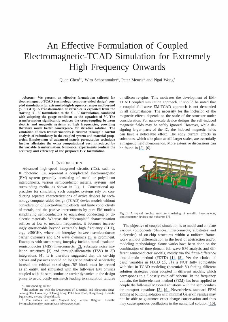
An Effective Formulation of Coupled Electromagnetic-TCAD Simulation for Extremely High Frequency Onward

An Effective Formulation of CoupledElectromagnetic-TCAD Simulation for Extremely

High Frequency OnwardsQuan Chen†∗, Wim Schoenmaker‡, Peter Meuris‡ and Ngai Wong†

Abstract—We present an effective formulation tailored forelectromagnetic-TCAD (technology computer-aided design) cou-pled simulations for extremely-high-frequency ranges and beyond(> 50GHz). A transformation of variables is exploited from thestarting A−V formulation to the E−V formulation, combinedwith adopting the gauge condition as the equation ofV . Thetransformation significantly reduces the cross-coupling betweenelectric and magnetic systems at high frequencies, providingtherefore much better convergence for iterative solution. Thevalidation of such transformations is ensured through a carefulanalysis of redundancy in the coupled system and material prop-erties. Employment of advanced matrix permutation techniquefurther alleviates the extra computational cost introduced bythe variable transformation. Numerical experiments confirm theaccuracy and efficiency of the proposed E-V formulation.

I. I NTRODUCTION

Advanced high-speed integrated circuits (ICs), such asRF/photonic ICs, represent a complicated electromagnetic(EM) system generally consisting of metal or polysiliconinterconnects, various semiconductor material systems, andsurrounding media, as shown in Fig. 1. Conventional ap-proaches for simulating such complex systems rely on con-ducting separate characterizations of active devices by tech-nology computer-aided design (TCAD) device models withoutconsideration of electrodynamic effects and finite conductivityof metals, and the passive interconnects by pure EM modelssimplifying semiconductors to equivalent conducting or di-electric materials. Whereas this “decoupled” characterizationsuffices at low to medium frequencies, it becomes increas-ingly questionable beyond extremely high frequency (EHF),e.g., >50GHz, where the interplay between semiconductorcarrier dynamics and EM wave dynamics [1] is prominent.Examples with such strong interplay include metal-insulator-semiconductor (MIS) interconnects [2], substrate noise iso-lation structures [3] and through-silicon-via (TSV) in 3Dintegrations [4]. It is therefore suggested that the on-chipactives and passives should no longer be analyzed separately;instead, the critical mixed-signal/RF block must be treatedas an entity, and simulated with the full-wave EM physicscoupled with the semiconductor carrier dynamics in the designphase to avoid costly mismatch leading to simulation failures

∗Corresponding author†The authors are with the Department of Electrical and Electronic Engi-

neering, The University of Hong Kong, Pokfulam Road, Hong Kong. E-mails:quanchen, [email protected]

‡ The authors are with Magwel NV, Leuven, Belgium. E-mails:wim.schoenmaker, [email protected]

or silicon re-spins. This motivates the development of EM-TCAD coupled simulation approach. It should be noted thata coupled full-wave EM-TCAD approach is not demandedin all circumstances. The necessity for the inclusion of themagnetic effects depends on the scale of the structure underconsideration. For nano-scale device designs the self-inducedmagnetic fields may be safely ignored. However, while de-signing larger parts of the IC, the induced magnetic fieldscan have a noticeable effect. The eddy current effects insubstrates, which take place at still larger scales, are essentiallya magnetic field phenomenon. More extensive discussions canbe found in [5], [6].

Fig. 1. A typical on-chip structure consisting of metallic interconnects,semiconductor devices and substrate [7].

The objective of coupled simulation is to model and emulatevarious components (devices, interconnects, substrates anddielectrics) of on-chip structures within a uniform frame-work without differentiation in the level of abstraction and/ormodeling methodology. Some works have been done on thecombination of time-domain full-wave EM analysis and dif-ferent semiconductor models, mostly via the finite-differencetime-domain method (FDTD) [1], [8]. Yet the choice ofbasic variables in FDTD (E, H) is NOT fully compatiblewith that in TCAD modeling (potentials V) forcing differentsolution strategies being adopted in different models, whichcorresponds to a ”loosely coupled” scheme. In the frequencydomain, the finite-element method (FEM) has been applied tocouple the full-wave Maxwell equations with the semiconduc-tor transport equations [2], [9]. Nevertheless, standard FEMaiming at building solution with minimal Galerkin residue maynot be able to guarantee exact charge conservation and thusmay cause spurious oscillations in the numerical solution [10].

2

A more sophisticated frequency-domain technique for multi-domain (metal, semiconductor and insulator) coupled simula-tion was proposed in [11], [12], based on the finite-volumemethod (FVM) that has built-in guarantee of charge conserva-tion. Instead of the conventional use of electric and magneticfields (E andH), the technique uses the scalar potentialV andvector potentialA (with B = ∇×A) as fundamental variables(denoted as A-V formulation or A-V solver hereafter), and asaconsequence provides a convenient, physically consistentand“tightly coupled” interfacing between the full-wave EM modeland the TCAD device model. The A-V formulation has beenvalidated for a number of cases in which the simulator resultswere compared with measured data on test structures devel-oped in industry [13], [14]. The solver has been transferredinto a series of commercial tools of MAGWEL [15].

Despite the attractive performance from DC to tens of GHz,the A-V solver suffers from a slow iterative solution in the highmicrowave and even terahertz (THz) regimes wherein EM-TCAD coupled simulation capacity is pressingly demanded.The high-frequency difficulty of A-V solver is attributed tothestrong cross-couplings between electric and magnetic systemsat high frequencies and when metallic materials are involved,which together lead to linear systems with significant off-diagonal dominance that largely affects the convergence ofiterative solvers.

In this paper, we propose a new framework of coupledsimulation characterized by usingV andE as basic variables,called the E-V formulation or solver henceforth, in the problemformulation, and by using a modified gauge condition as theequation ofV in metals and insulators. The transformationremoves much of the undesirable dependency of the cross-couplings on frequency and metal conductivity which is ingeneral a large variable. In this way the diagonal dominanceofresultant Jacobian matrices is improved and the performanceof iterative solution is greatly enhanced for EHF problems.Validity of the proposed E-V formulation is proved thoughexamining the redundancy problem specific to coupled sim-ulation and the influence of material properties. Additionalcost in computations introduced by the reformulation is wellalleviated by the column approximate minimum degree (CO-LAMD) permutation, rendering the E-V solver an effectivetool for generic integrated simulation tasks at sub-THz andTHz frequency ranges.

It should be emphasized that the E-V formulation obtainedby performing a variable transformation has interesting con-sequences for microelectronic applications. First, the minimalprocedure to identify voltages and currents at contacts andports is preserved. In other words, the connection to theKirchhoff variables is straightforward, as was discussed in[12]. Furthermore, the planar technology implies that currentelements in the vertical direction are usually over the lengthsof the via heights. Consequently, it is a valuable assumptionthat the vertical component of the vector potential is negligible.This approximation leads to a much smaller size of the set ofdegrees of freedom and this property is also preserved afterthe transformation. We also note that the resulting system isnot identical to the E-formulation that is often exploited infinite element solvers. The latter often works in the temporal

gauge for whichV = 0 everywhere.The remaining parts of the paper are organized as follows.

Section II briefly reviews the A-V formulation and verifies itsfeasibility with measurement data. Section III discusses theorigin of the difficulty that the A-V solver faces in iterativesolution at high frequencies. Formulation and implementationof the proposed E-V solver are detailed in Section IV. Anin-depth numerical study of the E-V solver including spectralanalyses is provided in Section V to demonstrate the meritsof the E-V solver. A conclusion is drawn in Section VI.

II. REVIEW OF A-V FORMULATION

A. A-V Formulation of the Coupled System

In the A-V framework for coupled simulation, the Gauss lawis used to solve for the scalar potentialV in insulating andsemiconducting regions, and the current-continuity equation∇ · J + jωρ = 0 is to employed to find theV in metals.

∇ ·[

εr(

∇V + jωA)]

+ ρ = 0 insul. & semi.∇ ·

[

(σ + jωεr)(

∇V + jωA)]

= 0 metal(1)

whereσ, εr andω denote respectively the conductivity, relativepermittivity, and frequency. The free charge density is denotedby ρ and in semiconductorsρ = n+p+Nd whereNd is the netdoping concentration. This set of equations is often regardedas the electric system.

The current-continuity equation is exploited to solve theelectron and hole charge carrier densities,n and p, in thesemiconductor region.

∇ · Jχ − jωqχ∓R(n, p) = 0, χ ∈ n, p , (2)

in which R(n, p) refers to the generation/recombination ofcarriers andq the elementary charge. The sign∓ is forelectrons and holes, respectively. Provided the drift-diffusionmodel is employed, the semiconductor current is determinedby Jχ = qµχχ (−∇V −jωA)±kTµχ∇χ, χ ∈ n, p, whereµ, k andT denote the carrier mobility, Boltzmann constant andtemperature, respectively. The Scharfetter-Gummel scheme isapplied to discretize (2) [16].

To solve the magnetic vector potentialA, we consider theMaxwell-Ampere equation, which is regarded as the magneticsystem

∇×

(

1

µr

∇× A

)

+K(σ + jωεr)(∇V + jωA)

−K Jsemi = 0,

(3)

whereJsemi = Jn+Jp denotes the semiconductor current, andK is the dimensionless constant in the scaling scheme [12].For generic materials of on-chip structures it is safe to setµr =1. Equation (3) itself is not well-defined since the operator∇× (∇×) is intrinsically singular when discretized by FVM.A special treatment in the A-V solver is to subtract (3) by thedivergence of the gauge condition

∇ · A+ ξKjωεrV = 0, (4)

which yields

∇×(

∇× A)

−∇(

∇ · A)

+K(σ + jωεr)jωA

+K(σ + jωεr)∇V − ξKjωεr∇V −KJsemi = 0,(5)

3

Fig. 2. View on the coupled spiral inductor using the MAGWEL editor.

whereξ is the gauge slider ranging from0 (Coulomb gauge)to 1 (Lorenz gauge). This regularization procedure recovers aLaplacian-like operator and thus eliminates the singularity.

The task of coupled simulation is to find the simultaneoussolution of (1), (2) and (5), which are represented in acondensed notation as

F(

V, n, p , A)

= 0

H(

V, n, p , A)

= 0

G(

V, n, p , A)

= 0

. (6)

B. Feasibility of the A-V Solver

Using the solver based on computational electrodynamics,we are able to compute the s-parameters by setting up a fieldsimulation of the full structure. This allows us to study indetail the physical coupling mechanisms. As an illustration,we consider two inductors which are positioned on a substratelayer separated by a distance of14µm. This structure wasprocessed and characterized and thes-parameters were ob-tained. It is quite convenient when studying a compact modelparameters to obtain a quick picture of the behavior of thestructure. For this device a convenient variable is the “gain”,which corresponds to the ratio of the injected power and thedelivered power over an output impedance [17]

G =Pin

Pout

. (7)

The structure is shown in Fig. 2.When computing thes-parameters, we put the signal source

on one spiral (port 1) and place50Ω impedance over thecontacts of the second spiral (port 2). Thes11-parameter isshown in Fig. 3 and thes12-parameter is shown in Fig. 4.Finally, the gain plot is shown in Fig. 5. This results shownhere have been obtained without any calibration of the materialparameters. The silicon is treated ’as-is’. This means thatthesubstrate and the eddy current suppressing n-wells are dealtwith as doped silicon.

III. O RIGIN OF THE HIGH-FREQUENCY BREAKDOWN OF

THE A-V SOLVER

The coupled system of equations (6) is intrinsically non-linear when semiconducting regions are present and preferably

-1.5

-1

-0.5

0

0.5

1

1.5

2

2.5

3

0 2e+09 4e+09 6e+09 8e+09 1e+10 1.2e+10 1.4e+10 1.6e+10

S1

1

f [Hz]

S11-abs-arg

S11 meas absS11 simul absS11 meas argS11 simul arg

Fig. 3. Comparison of the experiment and simulation results fors11 .

-2

-1.5

-1

-0.5

0

0.5

1

1.5

2

2.5

0 2e+09 4e+09 6e+09 8e+09 1e+10 1.2e+10 1.4e+10 1.6e+10

S1

2

f [Hz]

S12-abs-arg

S12 meas absS12 simul absS12 meas argS12 simul arg

Fig. 4. Comparison of the experiment and simulation results fors12 .

-100

-90

-80

-70

-60

-50

-40

-30

-20

1e+07 1e+08 1e+09 1e+10 1e+11

magnitude

frequency

Gain in dB

Gain measGain sim

Fig. 5. Comparison of the experimental and simulation results for the gain.

4

solved by the Newton’s method. The non-linearity arises fromthe discretization of the current flux along the links of thecomputational grid. As has been shown in [11], the discretizedcarrier current associated to a link of the grid is

Jχij = χiB(∓Xij)− χjB(±Xij), χ ∈ n, p (8)

whereχiandχj are the carrier concentrations of the begin andend nodes of the link, and

B(z) =z

exp(z)− 1(9)

is the Bernoulli function. The argumentXij = Vi − Vj +sgn(ij) jωhijAij andVi , Vj are the nodal voltages andAij

is the projection of the vector potentialA on the link< ij >.Finally sgn(ij) is ± depending on the orientation of the linkwith respect to its begin and end nodes. Evidently, the presenceof the Bernoulli function turns the problem into a highly non-linear one.

Starting from some initial guess, for example the DC solu-tion, the update vector in each Newton’s iteration is obtainedby solving the sparse linear system

MX = b, (10)

which in details reads

∂F∂V

∂F∂n,p

∂F∂A

∂H∂V

∂H∂n,p

∂H∂A

∂G∂V

∂G∂n,p

∂G∂A

∆V∆ n, p

∆A

= −

F(V, n, p , A)H(V, n, p , A)G(V, n, p , A)

.

(11)

The numerical difficulty of the A-V solver can be revealedby analyzing the magnitudes of the matrix entries in (11),which are mainly dependent on the electric properties of ma-terials and the frequency under consideration. The differentialoperators (∇,∇·,∇×) are usually of order one with spatialscaling. In the electric sector (1) the magnitude of the cross-coupling of A to V is

∂F

∂A= ∇ · [jω (σ + jωεr)] ∼ O (jω (σ + jωεr)) , (12)

whereO (·) denotes the order of the magnitude, and in themagnetic sector (5) the magnitude of the cross-coupling ofVto A is

∂G

∂V= [K(σ + jωεr)∇− ξKjωεr∇] ∼ O (K(σ + jωεr)) .

(13)Although the cross-couplings betweenA and V tend to

vanish at zero frequency, they become dominant for frequen-cies in the higher GHz range, especially when the structureincludes metallic conductors that have large conductivityσand skin effects are desired to be computed such that surface-impedance models can be obtained. When solved by thewidely-used Krylov subspace methods such as GMRES, thesesignificant off-diagonal blocks will impose negative effectsto the convergence rate through inducing undesirable spectraldistribution in the preconditioned system matrix. For instance,the popular ILU preconditioner and its variants compute theincompleteL andU factors ofM such that

M = LU + E, (14)

whereE is the error matrix. Then an iterative solver effectivelydeals with the preconditioned matrix

(LU)−1

M = I + U−1L−1E, (15)

For diagonally dominant matrices,L andU are well condi-tioned and the size (2-norm) ofU−1L−1E remains reasonablybounded, which confines the eigenvalues of the preconditionedmatrix within a small neighborhood of1 and allows a fastconvergence of Krylov subspace methods. When the matrixM lacks diagonal dominance,L−1 or U−1 may have largenorms, rendering the “preconditioned” error matrixU−1L−1Eof large size and thus adding large perturbations to the identitymatrix [18]. This large perturbation causes the eigenvalues dis-persed and spread far away from each other, resulting in slowdown or even failure of the convergence of iterative solution.As a consequence, the A-V solver becomes increasingly inef-ficient, if not impossible, in EHF scenarios wherein coupledsimulation is demanded to capture the complicated interplaybetween EM wave and semiconductor carrier transport.

IV. E-V FORMULATION

From a modeling perspective, the above intensive cross-coupling arise from explicitly separating the electric field(more precisely the electric field in the metals) into its staticcomponent fromV and dynamic component fromA, andassociating them with equal weightings that have magnitudesdepending on the frequency and metal conductivity. To reducethe weight of cross-coupling terms, we reformulate the coupledsystem using the scalar potentialV and the electric fieldEvia the variable transformation

E = −∇V − jωA. (16)

The coupled system of (1), (2) and (5) under this transfor-mation changes into

F′ :

∇ ·(

εrE)

+ ρ = 0, semi. & insul.

∇ ·[

(σ + jωεr) E]

= 0, metal(17a)

H′ : ∇ · Jχ − jωqχ∓R(n, p) = 0, χ ∈ n, p , (17b)

G′ : ∇×

(

∇× E)

−∇(

∇ · E)

+Kjω(σ + jωεr)E (17c)

−∇(

∇2V)

− ξKω2∇ (εrV ) +KjωJsemi = 0,

where Jχ = qµχχE ± kTµχ∇χ, χ ∈ n, p accordingly.Note that here we only considerE as a variable transformationof A instead of an independent physical quantity.

The transformation from A-V to E-V immediately removesthe conductance-dependent cross-coupling ofV from (17c).Yet little improvement has been made to (17a) wherein thecross-coupling coefficients ofE still have undesirable depen-dence onσ andω. A detailed analysis of the coupled systemin the next subsection however indicates that we are allowedtoexploit, instead of the Gauss law (17a) (as well as the current-continuity), the transformed gauge condition to determinethescalar potential in the metal and insulator regions (but notinthe semiconductor regions), which reads

∇2V + ξKω2εrV +∇ · E = 0. (18)

5

This way, the cross-couplings ofE have magnitudes of orderone, and are not growing any more with the large value ofσand frequency in the bulk of metallic materials. Whereas theconversion from A-V solver to E-V solver looks promising,there are certain subtleties that require special attention toguarantee a correct implementation of the E-V solver.

A. Redundancy in Coupled System

It is a unique feature for coupled EM-TCAD simulationto look for a simultaneous solution of the following system,which consists of the Gauss law, the current-continuity law,and the Maxwell-Ampere law

∇ · D − ρ = 0, (19a)

∇ · J = 0, (19b)

∇× H − J = 0, (19c)

whereJ represents the total current including the conductionand the displacement parts. In the A-V formulation all un-knowns are expressed in terms of potentialsV and A, and agauge condition is required to eliminate the well-known gaugefreedom to ensure a unique solution.

∇ · A+ f = 0 (20)

wheref can be an arbitrary function ofV and A.It is straightforward to see the system (19), more exactly

(19b) and (19c), is redundant by taking the divergence on bothsides of (19c) [19]. Conventional TCAD device simulation orfull-wave EM simulation alone, is free of this redundancy,in that the former uses only (19a) and (19b) to solve forVand ρ (n and p) without A, while the latter uses only (19c)and (20) to look forV and A in the absence ofρ (whichis recovered later via (19a)). When the A-V solver has todeal with the combined system of (19b) and (19c) that isfundamental to describe the field-carrier interaction, it employsa specific technique to address the redundancy problem, which,as mentioned above, is to subtract (19c) by the divergence ofthe gauge condition, yielding

∇× H − J −∇ ·(

∇ · A+ f)

= 0. (21)

There are several points in (21) that deserve attention: 1)The system of (19b) and (21) is not redundant as long as thegauge condition is not explicitly involved in the system ofequations; 2) Though the gauge condition does not participatein the solution procedure, it should serve as an implicitconstraint and be recovered from the solution thereby obtained.Taking divergence on (21) and together with (19b), we have

∇2(

∇ · A+ f)

= 0. (22)

which is essentially a Laplace’s equation. In numerical theory,it is known that for a Laplace’s equation∇2φ = 0 in somedomainΩ, the solution will be zero everywhere inΩ providedthe boundary conditionφ|∂Ω = 0 is applied. Hence therequirement of the second point is that the gauge conditionmust be set equal to zero at the boundary of the simulationdomain. This is done in the discretization of (21), wherein

the evaluations of∇ · A + f are forced to be equal tozero by the discretization scheme for the nodes bouncing onthe boundary of the simulation domain. In other words, thegauge condition will be automatically recovered over the usualMaxwell-Ampere equation for the whole domain provided thatthe current-continuity equation is solved.

Above discussion shows the way how the A-V solverdeals with the redundancy arising when different systems ofequations are coupled together, wherein the current-continuityequation is solved explicitly forV with the gauge conditionbeing an implicit constraint. Alternatively, one could choosethe gauge condition as the equation ofV constrained bythe current conservation. This change requires the current-continuity equation being removed from the system of equa-tions, otherwise the system will become redundant again sincethe gauge condition is enforced explicitly and implicitly atthe same time. The removal of current-continuity equationas a consequence requires the removal of charge densityρfrom the unknown list for an equal counting of equationsand unknowns. Such removal is applicable in the metallic andinsulating regions in whichρ is able to be recovered by theGauss law, while not in the semiconductors in which the carrierconcentrationsn andp are of fundamental interest and cannotbe recovered from merely the field variables.

As a result, in the E-V solver the equation (18) can beexploited to solve forV in the metals and insulators (thoughnot entirely, see the next section), while (17a) remains theonewe should use in the semiconducting regions. Note that thegauge condition will still be recovered in the semiconductorsgiven the fact that the gauge condition is set zero at all nodessurrounding the semiconductors. In addition, using (17) inthesemiconductors will not introduce large cross-coupling termsas the relative permittivities of semiconducting materials aregenerally of order one.

B. Issues of Material Properties

Depending on the electric properties of the materials underinvestigation (metal or insulator or material interfaces), thereare still subtle distinctions in the appropriate formulation ofgauge condition that should be employed as the equation ofV i.e., (18) in the E-V solver. For nodes in the bulk of metalsas well as material interfaces except semiconductor/insulatorinterfaces, the governing equation is essentially the current-continuity equation; the Gauss equation will come into useonly when the (surface) charge density is demanded in post-process steps. Therefore, the equation in the E-V solver forthese nodes is exactly (18), which together with (17c) areequivalent to the current-continuity equation (1) in the A-Vsolver.

The situation is slightly different for the insulating regions.The current-continuity is now trivial (0 = 0) and the (small-signal) free charge density is zero by definition. Therefore,there is no need to recover the current-continuity equationand only the Gauss’s equation must be recovered. Althoughapplying the gauge condition to find outV remains possible,such choice will induce certain numerical difficulty, especiallyfor the insulators with homogeneous dielectric constants.This

6

is because, due to the homogeneity of dielectric constants,solution of (18) in the bulk of insulators has to obey a strongerrequirement of demanding∇2V +KjωεrV = 0 and∇·E = 0simultaneously. Direct application of (18) will cause non-uniqueness in the solution and render the system matrix highlyill-conditioning. As a result, the ordinary Gauss equationremains an appropriate choice to determine the scalar potentialin the insulators, no matter homogeneous or inhomogeneous:

∇ ·(

εrE)

= 0. (23)

The nodes at semiconductor/insulator interfaces are classifiedas semiconductor nodes for which it is natural to apply theoriginal Gauss equation (17a).

C. Boundary Conditions

Boundary conditions for the E-V solver are derived fromits A-V counterpart through the transformation relation (16).The underlying principle is to minimize the coupling betweenthe simulation domain and the rest of the world.

As done in the A-V solver [11], [12], we divide the bound-ary of the simulation domain into two parts: contact regionsand non-contact regions. The contacts allow currents, and thusenergy, to enter and leave the simulation domain, whereinthe constant voltage condition is applied. The remainder, thenon-contact boundary, is characterized by demanding thatthe outward-pointing normal component ofE vanishes, i.e.,En = 0. This leads to the boundary condition of the electricsystem for non-contact boundary nodes:

∇ ·[

(σ + jωεr) E]

= 0. (24)

The boundary condition (24) introduces again aσ-dependentcoupling in some circumstances, i.e., for boundary nodesattached by metallic cubes. Their contribution to undesirablecross-couplings, however, is much lower than that in the A-V formulation, wherein all nodes attached by metallic cubeshave to be taken into account.

For the magnetic sector, the similar requirement ofBn = 0is applied to keep all magnetic fields remain inside thesimulation domain. This forces a zero tangential componentof A since B = ∇ × A, viz. At = 0, which holds for boththe contact and non-contact boundaries. In light of (16), theboundary condition of magnetic system should be

Et = −∇Vt. (25)

The above condition implies the unknowns associated to theboundary links, which are part of degrees of freedom in theE-V solver but not in the A-V solver, can be substituted by thecorresponding nodal unknowns ofV in the solution phase andrecovered later by post-processing. This way, the total numberof unknowns are identical for both the A-V and E-V solvers.

It should be emphasized that above selection of the bound-ary conditions represents a particular choice which was moti-vated by upgrading standard TCAD simulations into the elec-tromagnetic regime. However, there is nothing “fundamental”about this choice. One may equally well choose radiativeboundary conditions or Neumann-type boundary conditionsfor the vector potential. The preferred choice depends on the

problem under consideration. Here, it is important to note thatwhen discussing the A-V solver and the E-V solver, thesamephysical boundary conditions are used.

D. Implementation Details

The full system of equations of the E-V solver is laid outin (26).

F′ :

∇ ·[

(σ + jωεr) E]

− ρ = 0, boundary.

∇ ·(

εrE)

− ρ = 0, Semi. and insul.

∇2V + ξKω

2εrV +∇ · E = 0, remaining regions.

(26a)

H′ : ∇ · Jχ − jωqχ∓R(n, p) = 0, χ ∈ n, p , (26b)

G′ : ∇×

(

∇× E)

−∇(

∇ · E)

+Kjω(σ + jωεr)E (26c)

−∇(

∇2V)

− ξKω2∇ (εrV ) +KjωJsemi = 0,

Similar to (11), a linear systemMX = b is solved ateach Newton’s step, in whichM results from the FVMdiscretization of the Jacobian of (26).

It is convenient to upgrade the A-V solver to include an E-Vsolver by exploiting the following 4-step solution strategy:

1) Map A− V variables ontoE − V variables via (16).2) Apply the E-V solver to compute the update vector

[

∆V,∆E]T

in the Newton’s iteration.

3) Map[

∆V,∆E]T

onto[

∆V,∆A]T

4) Update the A-V system.

Using this approach, the data structure in the original A-Vsolver is unaltered and the switching between the A-V andE-V solvers is easy to realize. This is beneficial in that, asshown in Section IV, the A-V and E-V solvers are suitableto work complementarily with the former at low frequenciesand the latter at high frequencies, and thus switching betweensolvers may be needed in a wide-band simulation.

E. Matrix Permutation

Despite the attractive reduction in the magnitudes of cross-couplings, the E-V transformation introduces more non-zerofill-ins into the off-diagonal block of∂G

∂Vthrough the term

∇(

∇2V)

in (26c). The increased amount of fill-ins from A-V to E-V formulations is approximately10× the number ofboundary links. Inferior sparsity burdens the construction ofpreconditioner as well as subsequent iterations, limitingtheapplications of E-V solver to relatively small-sized problems.

To enhance the performance of the E-V solver, the columnapproximate minimum degree (COLAMD) permutation [20]is applied to the system matrixM , which computes a permu-tation vectorp such that the (incomplete) LU factorization ofM(:, p) tends to be much sparser than that ofM . This way,building popular ILUT preconditioners with small thresholdbecomes possible forM in the order of tens of thousands.The subsequent iteration also speeds up owing to the improvedsparsity of the computed LU factors.

7

(a) (b)

Fig. 6. (a) Cross wire structure. Simulation domain is10× 10× 10µm3 andthe cross sections of metal wires are2× 2µm2. σ = 5.96× 107S/m. FVMdiscretization generates1400 nodes and3820 links. (b) Metal plug structure.Simulation domain is10 × 10 × 10µm3 the cross section of metal plug is4× 4µm2. σ = 3.37× 107S/m. A uniform doping ofND = 1× 1024 isused. FVM discretization generates1300 nodes and3540 links.

V. NUMERICAL RESULTS

The proposed E-V solver as well as its A-V counterpart, onwhich MAGWEL’s softwares are based, are implemented andcompared in MATLAB. The “de Mari” scaling scheme [12] isadopted. For simplicity, the Coulomb gauge (ξ = 0) is adoptedthroughout the numerical experiments. Three structures aretested to demonstrate the efficiency of the E-V solver: 1)a cross wire structure consisting only passives as shownin Fig. 6(a); 2) a metal plug structure consisting of bothpassives and actives as shown in Fig. 6(b); 3) a practicalsubstrate noise isolation (SNI) structure as shown in Fig. 7.The iterative solutions are computed by GMRES with ILUTpreconditioners. All programming and simulations were doneon a3.2GHz 16Gb-RAM Linux-based server.

Fig. 7. Substrate noise isolation structure. A deep n-well (DNW) (pink region)is implanted in the p-type substrate to isolate analog circuits from digital noisesources. Simulation domain is100 × 50 × 11µm3. σ = 3.37 × 107S/m.A user-defined doping profile is adopted. FVM discretizationgenerates6300nodes and13540 links.

A. Accuracy of E-V Solver

Fig. 8 verifies the accuracy of E-V solver in comparisonwith the A-V solver at frequencies ranging from106Hz to1015Hz for the three test benches. This frequency range

covers a wide spectrum from medium radio frequency tovisible light. Direct solver (Gaussian elimination) is used tosolve the linear equations at each Newton’s iteration. Theaccuracy is measured by the relative error between the wholeinternal state space solution of the A-V and E-V solverserr = ‖XEV −XAV ‖2 / ‖XAV ‖2, X =

[

V ;n; p; A]

. It isseen that the E-V solver is in an excellent agreement withthe A-V solver throughout the testings, which is expectedfrom a mathematical perspective since no approximation isintroduced in the variable and equation transformations. Theslight fluctuations in the curves are due to the final precisionsof Newton’s method and vary among solvers even whenthe same convergence criterion is applied. Fig. 9 visualizesthe current density inside the substrate of the SNI structure,demonstrating a clear isolation effect for the part of analogcircuits from external digital noises.

106

108

1010

1012

1014

1016

10−16

10−14

10−12

10−10

10−8

10−6

10−4

10−2

100

Frequency (Hz)

Err

or

Cross wire

Metal plug

SNI

Fig. 8. Differences between the A-V and E-V solvers for the testing structures(with direct solver).

0 1 2 3 4 5 6 7 80

0.5

1

1.5

2

2.5

3

3.5

4

0

1

2

3

4

5

6

Fig. 9. Current density at the middle layer of the substrate ofSNI structure(shown in log10 scale).

B. Spectral Analyses

To investigate the influence of increasing frequency onthe A-V and E-V solvers, we plot in Fig. 10 and Fig. 11the eigenvalues of the Jacobian matrices preconditioned by

8

TABLE INORMS OFL−1 AND U−1 COMPUTED FOR THEA-V AND E-V SOLVERS

(ILUT(10−6))

FrequencyA-V E-V

∥

∥L−1∥

∥

∥

∥U−1∥

∥

∥

∥L−1∥

∥

∥

∥U−1∥

∥

106Hz 1.55× 101 4.82 9.15× 101 1.67× 107

109Hz 1.32× 101 4.87× 102 4.37× 101 3.82× 104

1012Hz 2.50× 101 1.75× 107 2.89× 101 1.16× 102

1015Hz 2.42× 102 1.15× 1011 1.52× 101 5.15

ILUT(10−6) for the metal plug structure at four differentfrequencies. The norms ofL−1 andU−1 of each solver arealso computed in Table I.

0.9 0.95 1 1.05 1.1−5

0

5x 10

−3 106 Hz

−300 −200 −100 0 100−40

−20

0

20109 Hz

−1 0 1 2

x 106

−2

−1

0

1x 10

6 1012 Hz

−2 0 2 4 6

x 1012

−2

−1

0

1

2x 10

12 1015 Hz

Fig. 10. Eigenvalue distribution of the preconditioned Jacobian matrices ofA-V solver at different frequencies.

−400 −200 0 200 400−400

−200

0

200106 Hz

−10 0 10 20−10

−5

0

5

10109 Hz

0 0.5 1 1.5 2−1

−0.5

0

0.5

11012 Hz

0.8 1 1.2 1.4−0.5

0

0.51015 Hz

Fig. 11. Eigenvalue distribution of the preconditioned Jacobian matrices ofE-V solver at different frequencies.

At relatively low frequency (106Hz), the off-diagonal blocksin (12) and (13) are of small sizes and so are the normsof the inverses of incomplete factorsL and U in (15). Theeigenvalues of the preconditioned matrix from the A-V solverare then tightly clustered around the point1 in favor of a fastconvergence of iterative solution. As frequency increases, thespectra of the preconditioned matrices have eigenvalue clusterswith continuously enlarging radii and separations among each

0.99 0.995 1 1.005 1.01−0.01

−0.005

0

0.005

0.01106 Hz

0.9 0.95 1 1.05 1.1−5

0

5x 10

−3 109 Hz

−1 0 1 2 3−0.5

0

0.51012 Hz

−5 0 5 10−10

0

10

201015 Hz

Fig. 12. Eigenvalue distribution of the preconditioned Jacobian matrices ofA-V solver at different frequencies (no metal).

0.9 1 1.1 1.2−0.05

0

0.05106 Hz

0.9 1 1.1 1.2−0.05

0

0.05109 Hz

0.9 1 1.1 1.2−0.05

0

0.051012 Hz

0.9 1 1.1 1.2 1.3−0.1

−0.05

0

0.05

0.11015 Hz

Fig. 13. Eigenvalue distribution of the preconditioned Jacobian matrices ofE-V solver at different frequencies (no metal).

other, reflecting an increasing perturbation to the identitymatrix as the result of increasing off-diagonal dominance.Thisis also confirmed by looking into the growing sizes ofU−1

in Table I. It therefore suggests a poor iterative performancefor the A-V solver at high frequencies when Krylov subspacemethods are applied, whose convergence behaviors are closelyrelated to the relative radii of eigenvalue clusters and their sep-arations of the preconditioned matrix [21]. The enlargementsof cluster radii and separations are proportional to the increasesof frequency.

Compared to that of the A-V solver, the spectral distributionof the preconditioned system of E-V solver has a roughlyopposite trend along with the rising frequency. The eigenvaluesare clustered more loosely at low frequencies, while becomingincreasingly concentrated around1 at higher frequencies, dueto the growing contribution from the term ofKjω(σ+jωεr)Ein (26c) improving diagonal dominance. Such concentrationof eigenvalues greatly facilitates the convergence of iterativemethods and thus suggests enhanced performances for the E-Vsolver at high-frequency scenarios.

Similar experiments are conducted in Fig. 12 and Fig. 13to examine the role of metal conductivity. The metal plug

9

structure is used again, but with the metallic part replacedbyinsulating materials, rendering the structure consistingof onlyinsulators and semiconductors. Horizontal comparisons for theA-V solver show that, whereas at sufficiently high frequenciesthe eigenvalues still disperse, the degree of dispersion isreduced by a great extent. This confirms that the presenceof metallic conductors with large conductivity is one originof the numerical difficulty of A-V solver at high frequencies.The eigenvalues of E-V solver are in a similar distributionover the four testing frequencies, suggesting roughly constantperformance in iterative solution.

C. Performance Comparisons

Detailed comparisons between the A-V and E-V solversfor their performances in iterative solution are tabulatedinTable II-IV. A relative tolerance of10−10 and a maximumnumber of iterations of1000 are used in GMRES. The highaccuracy used in iterative solution is intended to minimizethenumber of necessary Newton iterations to as close as withdirect solver, so as not to complicate the analysis by theissues related to the convergence rate of Newton’s method.Successful solutions with convergence achieved are shownwith the time for building preconditioner, the number ofiterations and the time per iteration. Unsuccessful solutions,according to the reasons of failure, are marked as “NC” (noconvergence within the maximum number of iterations) or“IP” (ill-conditioned preconditioner). The iterative solvers withand without COLAMD pre-processing are labeled as “AMD”and “ORIG”, respectively. The runtimes of direct solver (at10GHz) are also shown with the label of “DS” for reference.

For all the three structures, the A-V solver exhibits deterio-rated performances as frequency increases, and tends to breakdown at frequencies beyond (tens of) GHz for requiring eithera large number of iterations or high-quality preconditionersthat are costly to generate (“UV catastrophe”). The E-V solverfails to converge for low frequencies (“IR singularity”) but incontrast to the A-V solver, performs increasingly well withgrowing frequency. These results are consistent with the abovespectral analysis and confirm the merit of the E-V solver asa capable tool in EHF applications. Meanwhile, it suggeststhat the A-V and E-V solvers have complementary preferablefrequency ranges and thus are suitable to work together toprovide a truly wide-band coupled simulation framework.

As frequency increases, calculating ILUT preconditionersare generally more time-consuming for the A-V solver, whileless for the E-V solver, which may be attributed to theiropposite behaviors in terms of diagonal dominance. Withoutmatrix permutation, the constructions of preconditionersforthe E-V solver is several times slower than that of the A-Vsolver due to a higher number of matrix fill-ins introduced bythe ∇(∇2V ) term. This prevents the E-V solver from beingapplied to simulate large-scale problems. As a remedy, applica-tion of the COLAMD permutation in the E-V solver providesa remarkable reduction (∼ 20X for the SNI example) in thecomputational cost of preconditioner and a moderate reduction(> 2X for the SNI example) in the cost of following iterations,rendering the overall cost of E-V solver comparable even

with that of the COLAMD-permuted A-V solver, for whichthe improvement is less significant because of its inherentlybetter sparsity. Besides, an increased number of iterations isobserved for the COLAMD-permuted A-V solver comparedto the original version, offsetting its gain in preconditionercomputations. It turns out that the E-V solver combined withCOLAMD is the most robust and efficient tool for coupledsimulations at EHF and beyond.

VI. CONCLUSION

An effective E-V formulation is proposed, with dedicationto the simultaneous simulation of full-wave EM and semi-conductor dynamics for EHF regime onwards. The underlyingidea is to reformulate the conventional A-V formulation viavariable and equation transformations, which removes theundesirable dependencies of cross-couplings on frequencyandmetal conductivity, and as a consequence brings substantialimprovement into the efficiency of iterative solution at highfrequencies. From a spectral perspective, the improved di-agonal dominance ameliorates the concentric appearance ofeigenvalues of the preconditioned Jacobian matrix, by whicha fast convergence of iterative solution is achieved. Theequation transformation from the Gauss equation to the gaugecondition is rigorously validated by a careful investigation ofthe redundancy in coupled system and the influence of materialproperties. The COLAMD matrix permutation technique isapplied to offset the additional cost introduced by the E-Vreformulation, rendering the E-V solver comparably efficientwith its A-V counterpart. Numerical experiments have con-firmed the superior performance of the proposed method withfrequency up to optical range.

ACKNOWLEDGEMENT

This work was supported in part by the Hong Kong Re-search Grants Council under Projects HKU 717407E and718509E, the University Research Committee of The Uni-versity of Hong Kong, and in part by the EU projectsCHAMELEON-RF (IST-2004-027378), ICESTARS (IST-FP7/2008/ICT/214911) and the IWT-Medea + project COSIP-Vlaanderen (IWT-080478). Discussions with Nicodemus Ba-nagaaya and Wil Schilders are highly appreciated.

REFERENCES

[1] K. J. Willis, J. S. Ayubi-Moak, S. C. Hagness, and I. Knezevic,“Global modeling of carrier-field dynamics in semiconductors usingEMC-FDTD,” Journal of Computational Electronics, vol. 8, no. 2, pp.153–171, Jun 2009.

[2] G. F. Wang, R. W. Dutton, and C. S. Rafferty, “Device-level simula-tion of wave propagation along metal-insulator-semiconductor intercon-nects,”IEEE Trans. Microw. Theory Tech., vol. 50, no. 4, pp. 1127–1136,Apr 2002.

[3] P. C. Yeh, H. K. Chiou, C. Y. Lee, J. Yeh, D. Tang, and J. Chern,“An experimental study on high-frequency substrate noise isolation inBiCMOS technology,”Electron Device Letters, IEEE, vol. 29, no. 3, pp.255–258, March 2008.

[4] C. Xu, H. Li, R. Suaya, and K. Banerjee, “Compact AC modelingandanalysis of Cu, W, and CNT based through-silicon vias (TSVs) in 3-DICs,” in Proc. IEEE Electron Device Meeting (IEDM), 2009, pp. 521–524.

10

TABLE IIITERATIVE PERFORMANCE OFA-V AND E-V SOLVERS FOR THE CROSS WIRE STRUCTURE. (ILUT(10−6), TIME UNIT : SECOND)

Freq.A-V(ORIG) A-V(AMD)

A-V(DS)E-V(ORIG) E-V(AMD)

E-V(DS)tpre Nit tper it tpre Nit tper it tpre Nit tper it tpre Nit tper it

106 48.34 5 0.37 11.22 5 0.38

12.76

NC NC

15.08

107 62.15 6 0.34 12.68 7 0.37 179.16 546 1.51 49.88 515 1.01108 62.96 11 0.41 12.91 12 0.39 179.49 130 1.11 45.73 91 0.71109 77.59 27 0.42 14.80 35 0.41 163.00 17 1.09 43.15 14 0.671010 105.06 43 0.73 20.77 167 0.50 163.73 9 1.09 38.01 8 0.651011 NC NC 155.41 8 1.03 38.09 7 0.631012 NC NC 154.45 7 1.01 38.50 7 0.611013 IP NC 154.52 7 1.08 38.77 6 0.571014 IP IP 150.29 6 0.98 34.55 6 0.571015 IP IP 127.37 5 1.01 28.64 6 0.51

TABLE IIIITERATIVE PERFORMANCE OFA-V AND E-V SOLVERS FOR THE METAL PLUG STRUCTURE. (ILUT(10−6), TIME UNIT : SECOND)

Freq.A-V(ORIG) A-V(AMD)

A-V(DS)E-V(ORIG) E-V(AMD)

E-V(DS)tpre Nit tper it tpre Nit tper it tpre Nit tper it tpre Nit tper it

106 100.02 5 0.57 34.83 5 0.62

37.39

NC NC

50.12

107 146.18 6 0.54 53.71 7 0.65 NC NC108 156.44 10 0.60 62.01 11 0.68 616.12 187 2.11 136.12 141 1.11109 200.28 22 0.69 62.50 27 0.66 455.02 81 1.81 129.19 51 0.911010 207.16 102 0.73 69.39 165 0.72 442.65 21 1.73 128.94 18 0.921011 NC NC 440.56 13 1.72 100.18 12 0.801012 NC NC 369.19 11 1.39 85.50 11 0.781013 IP NC 363.20 9 1.32 83.16 10 0.781014 IP IP 362.21 7 1.23 83.18 7 0.811015 IP IP 309.64 5 1.10 83.20 6 0.74

TABLE IVITERATIVE PERFORMANCE OFA-V AND E-V SOLVERS FOR THESNI STRUCTURE. (ILUT(10−4), TIME UNIT : SECOND)

Freq.A-V(ORIG) A-V(AMD)

A-V(DS)E-V(ORIG) E-V(AMD)

E-V(DS)tpre Nit tper it tpre Nit tper it tpre Nit tper it tpre Nit tper it

106 1298.45 8 2.57 252.83 9 2.12

943.01

NC NC

1391.67

107 1506.15 32 3.54 349.11 41 3.45 NC NC108 2112.06 100 4.60 539.78 140 4.08 NC NC109 NC NC 17347.12 141 11.12 770.81 101 3.621010 NC NC 13556.65 71 9.34 598.76 70 3.491011 NC NC 9342.33 47 9.02 474.05 44 3.281012 IP NC 8006.09 40 8.62 427.25 36 3.201013 IP IP 7681.85 36 8.00 394.00 32 3.011014 IP IP 7262.10 19 7.68 318.64 18 2.851015 IP IP 7245.72 16 6.11 301.66 15 2.79

[5] W. Schoenmaker, P. Meuris, E. Janssens, W. Schilders, andD. Ioan,“Modeling of passive-active device interactions,” inProc. 37th Euro-pean Solid-State Device Research Conference, ESSDERC-2007, MunichGermany, Sept. 2007.

[6] N. Nastos and Y. Papananos, “RF optimization of MOSFETs under in-tegrated inductors,”IEEE Trans. on Microwave Theory and Techniques,vol. 54, no. 5, pp. 2106–2117, 2006.

[7] S. Kapora, M. Stuber, W. Schoenmaker, and P. Meuris, “Substrate noiseisolation characterization in 90nm CMOS technology,” inUser trackIEEE Design Automation Conference (DAC), 2009.

[8] R. O. Grondin, S. M. El-Ghazaly, and S. Goodnick, “A review ofglobal modeling of charge transport in semiconductors and full-waveelectromagnetics,”IEEE Trans. Microw. Theory Tech., vol. 47, no. 6,pp. 817–829, Jun 1999.

[9] F. Bertazzi, F. Cappelluti, S. D. Guerrieri, F. Bonani, and G. Ghione,“Self-consistent coupled carrier transport full-wave EM analysis ofsemiconductor traveling-wave devices,”IEEE Trans. Microw. TheoryTech., vol. 54, no. 4, pp. 1611–1617, Apr 2006.

[10] W. Schoenmaker, W. Magnus, P. Meuris, and B. Maleszka, “Renormal-ization group meshes and the discretization of TCAD equations,” IEEETrans. Comput.-Aided Design, vol. 21, no. 12, Dec 2002.

[11] P. Meuris, W. Schoenmaker, and W. Magnus, “Strategy for electro-magnetic interconnect modeling,”IEEE Trans. Comput.-Aided Design,vol. 20, no. 6, pp. 753–762, Jun. 2001.

[12] W. Schoenmaker and P. Meuris, “Electromagnetic interconnects and pas-

sives modeling: software implementation issues,”IEEE Trans. Comput.-Aided Design, vol. 21, no. 5, pp. 534–543, May 2002.

[13] CODESTAR - compact modeling of on-chip passive structures at highfrequencies. [Online]. Available: http://www.magwel.com/codestar/

[14] Chameleon-RF - comprehensive high-accuracy modeling ofelectromagnetic effects in complete nanoscale RF blocks. [Online].Available: http://www.chameleon-rf.org/

[15] Magwel. [Online]. Available: http://www.magwel.com/[16] D. L. Scharfetter and H. K. Gummel, “Large scale analysis of a silicon

read diode oscillator,”IEEE Trans. Electron Devices, vol. 16, no. 1, pp.64–77, Jan. 1969.

[17] A. M. Niknejad and R. G. Meyer, “Analysis, design and optimizationof spiral inductors and transformers for Si RF ICs,”IEEE Journ. ofSolid-State Circuits, vol. 33, pp. 1470–1481, 1998.

[18] Y. Saad,Iterative methods for sparse linear systems. Boston: PWS,1996.

[19] P. Enders, “Underdeterminacy and redundance in Maxwell’s equationsequations. Origin of gauge freedom - transversality of freeelectro-magnetic waves - Gaugefree canonical treatment without constraints,”Electronic Journal of Theoretical Physics, vol. 6, no. 22, pp. 135–166,Oct. 2009.

[20] T. A. Davis, J. R. Gilbert, S. I. Larimore, and E. G. Ng, “A columnapproximate minimum degree ordering algorithm,”ACM Trans. Math.Softw., vol. 30, no. 3, pp. 353–376, 2004.

11

[21] S. L. Campbell, I. C. F. Ipsen, C. T. Kelley, and C. D. Meyer, “GMRESand the minimal polynomial,”BIT, vol. 36, pp. 32–43, 1996.