An Efﬁcient Hybrid Algorithm for the Separable Convex ...users.clas.ufl.edu/hager/papers/CG/knapsack.pdf · Additional Key Words and Phrases: Continuous quadratic knapsack, nonlinear

22

An Efficient Hybrid Algorithm for the Separable Convex QuadraticKnapsack Problem

TIMOTHY A. DAVIS, Texas A&M UniversityWILLIAM W. HAGER, University of FloridaJAMES T. HUNGERFORD, M.A.I.O.R.

This article considers the problem of minimizing a convex, separable quadratic function subject to a knapsackconstraint and a box constraint. An algorithm called NAPHEAP has been developed to solve this problem.The algorithm solves the Karush-Kuhn-Tucker system using a starting guess to the optimal Lagrangemultiplier and updating the guess monotonically in the direction of the solution. The starting guess iscomputed using the variable fixing method or is supplied by the user. A key innovation in our algorithm isthe implementation of a heap data structure for storing the break points of the dual function and computingthe solution of the dual problem. Also, a new version of the variable fixing algorithm is developed that isconvergent even when the objective Hessian is not strictly positive definite. The hybrid algorithm NAPHEAPthat uses a Newton-type method (variable fixing method, secant method, or Newton’s method) to bracket aroot, followed by a heap-based monotone break point search, can be faster than a Newton-type method byitself, as demonstrated in the numerical experiments.

CCS Concepts: � Mathematics of computing → Mathematical analysis; Mathematical optimiza-tion; Continuous optimization; Quadratic programming

Additional Key Words and Phrases: Continuous quadratic knapsack, nonlinear programming, convex pro-gramming, quadratic programming, separable programming, heap

ACM Reference Format:Timothy A. Davis, William W. Hager, and James T. Hungerford. 2016. An efficient hybrid algorithm for theseparable convex quadratic knapsack problem. ACM Trans. Math. Softw. 42, 3, Article 22 (May 2016), 25pages.DOI: http://dx.doi.org/10.1145/2828635

1. INTRODUCTION

We consider the following separable convex quadratic knapsack problem:

minx∈Rn

q(x) := 12

xTDx − yTx (1)

subject to � ≤ x ≤ u and r ≤ aTx ≤ s,

The authors gratefully acknowledge support by the Office of Naval Research under Grants No. N00014-11-1-0068 and No. N00014-15-1-2048, by the National Science Foundation under Grants No. 0620286 and No.1522629, and by the Defense Advanced Research Project Agency under Contract No. HR0011-12-C-0011.The views, opinions, and/or findings contained in this article are those of the authors and should not beinterpreted as representing the official views or policies of the Department of Defense or the U.S. Government.Distribution Statement “A” (Approved for Public Release, Distribution Unlimited).Authors’ addresses: T. A. Davis, 425E HRBright Building, Department of Computer Science and Engi-neering, Texas A&M University, 3112 TAMU, College Station, TX 77843-3112; email: [email protected]; W.W. Hager, Department of Mathematics, University of Florida, 358 Little Hall, PO Box 118105, Gainesville,FL 32611-8105; email: [email protected]; J. T. Hungerford, M.A.I.O.R. – Management, Artificial Intelligence,and Operations Research, Lucca, Italy; email: [email protected] to make digital or hard copies of all or part of this work for personal or classroom use is grantedwithout fee provided that copies are not made or distributed for profit or commercial advantage and thatcopies bear this notice and the full citation on the first page. Copyrights for components of this work ownedby others than the author(s) must be honored. Abstracting with credit is permitted. To copy otherwise, orrepublish, to post on servers or to redistribute to lists, requires prior specific permission and/or a fee. Requestpermissions from [email protected] Copyright is held by the owner/author(s). Publication rights licensed to ACM.ACM 0098-3500/2016/05-ART22 $15.00DOI: http://dx.doi.org/10.1145/2828635

ACM Transactions on Mathematical Software, Vol. 42, No. 3, Article 22, Publication date: May 2016.

http://dx.doi.org/10.1145/2828635

http://dx.doi.org/10.1145/2828635

22:2 T. A. Davis et al.

where a, y ∈ Rn, � ∈ (R ∪ {−∞})n, u ∈ (R ∪ {∞})n, r, s ∈ R, and D ∈ R

n×n is a positivesemidefinite diagonal matrix with diagonal d. Without loss of generality, we assumethat � < u. Problem (1) has applications in quadratic resource allocation [Bitran andHax 1981; Bretthauer and Shetty 1997; Cosares and Hochbaum 1994; Hochbaum andHong 1995], quasi-Newton updates with bounds [Calamai and More 1987], multi-capacity network flow problems [Helgason et al. 1980; Nielsen and Zenios 1992; Shettyand Muthukrishnan 1990], continuous formulations of graph partitioning problems[Hager and Hungerford 2015; Hager and Krylyuk 1999], and support vector machines[Dai and Fletcher 2006].

By introducing an auxiliary variable b ∈ R, we may reformulate Problem (1) as:

minx∈Rn, b∈R

{q(x) : � ≤ x ≤ u, r ≤ b ≤ s, aTx = b}. (2)

Making the substitutions

x ←(

xb

), � ←

(�r

), u ←

(us

), a ←

(a

−1

), n ← n + 1,

and augmenting y and d by an additional zero entry, Problem (2) is transformed intothe problem

minx∈Rn

{q(x) : � ≤ x ≤ u, aTx = 0}.Hence, without loss of generality, we may restrict our study to an equality-constrainedversion of Problem (1):

minx∈Rn

{q(x) : � ≤ x ≤ u, aTx = b}, (3)

where b ∈ R is given. The constraints of Problem (3) are continuous analogs of theconstraints that arise in the discrete knapsack problem (see Bretthauer et al. [1996]).

In quadratic resource allocation, problem (3) arises with a = 1 and � = 0, where 1and 0 are the vectors whose entries are all 1 and 0, respectively. The objective is tominimize the total cost of allocating b resources to n projects, where 1

2 dix2i − yixi is the

cost function for project i. The amount of resources allocated to project i is constrainedto lie between �i and ui.

In other applications [Calamai and More 1987; Dai and Fletcher 2006; Hager andHungerford 2015; Hager and Krylyuk 1999; Helgason et al. 1980; Nielsen and Zenios1992; Shetty and Muthukrishnan 1990], an objective function F is minimized over afeasible set described by bound constraints and a single linear equality constraint:

minx∈Rn

{F(x) : � ≤ x ≤ u, aTx = b}. (4)

The gradient projection algorithm as formulated in Hager and Zhang [2006] startswith an initial guess x0 ∈ R

n to a solution of (4), and for each k ≥ 0, the (k+ 1)st iterateis given by

xk+1 = xk + skpk, where pk = proj(xk − αk∇F(xk)).

Here sk ≥ 0 is the stepsize, αkI is an approximation to the inverse Hessian of F, andproj(z) is the unique projection, relative to the 2-norm, of z onto the feasible set of (4).That is, proj(z) is the solution of the problem

minx∈Rn

{12

‖x − z‖2 : � ≤ x ≤ u, aTx = b}

. (5)

This projection problem is a special case of Problem (3) in which D is the identitymatrix and y = xk − αk∇F(xk).


Separable Convex Quadratic Knapsack Problem 22:3

Specialized algorithms for solving (3) typically assume D is positive definite andsearch for a root of the derivative of the dual function, a continuous piecewise linear,monotonic function with at most 2nbreak points (“kinks” where the slope could change).The first algorithm [Helgason et al. 1980] was based on sorting all the break pointsand then sequentially marching through the break points until the optimal multiplierwas found. The worst case complexity of this algorithm is O(n log2 n) due to the sort.Starting with Brucker [1984], linear time algorithms were proposed based on a mediansearch rather than a sort. Subsequent developments of the median search methodinclude those in Calamai and More [1987], Maculan et al. [2003], and Pardalos andKovoor [1990].

Bitran and Hax [1981] proposed a method for solving a generalization of Problem (3)in which the objective function is convex and separable but not necessarily quadratic.In their algorithm, which has come to be known as the variable fixing method, eachiteration implicitly computes an estimate for the optimal Lagrange multiplier by solv-ing a subproblem in which the box constraints are ignored. Based on the sign of thederivative of the dual function at the multiplier estimate, a non-empty subset of indicesis identified for which xi can be optimally fixed at an upper or lower bound. The fixedvariables are removed from the problem and the process repeats until all the boundcomponents of an optimal solution have been determined. Subsequent developmentsof this approach in the context of Problem (3) can be found in Bretthauer et al. [1996],Kiwiel [2008], Michelot [1986], Robinson et al. [1992], Shor [1985], and Ventura [1991].An efficient and reliable implementation of the variable fixing method for Problem (3),and a thorough convergence analysis, is given by Kiwiel [2008].

Dai and Fletcher [2006] developed a method in which each multiplier estimate is theroot of a secant approximation to the derivative of the dual function (with additionalmodifications for speeding up convergence). In Cominetti et al. [2014], a method isproposed by Cominetti, Mascarenhas, and Silva that uses semi-smooth Newton stepsfor updating multiplier estimates, with a secant safeguard. Numerical experimentsusing a standard test set of randomly generated problems showed that the semi-smoothNewton method was faster than the variable fixing method, the secant method, and amedian-based method. As we explain in Section 3, Newton’s method is not very wellsuited for problems where the elements of d are small relative to elements of y sincethe derivative of the dual function is nearly piecewise constant, and when a Newtoniterate lands on a flat segment, it jumps towards ±∞. As shown in Cominetti et al.[2014], if a > 0 and u = ∞ or � = −∞, then the variable fixing method and Newton’smethod can generate identical iterates. This result is generalized in Section 2.

In this article we develop an algorithm called NAPHEAP that is built around amonotone break point search implemented using a heap data structure. Given aninterval (α, β) containing an optimal dual multiplier λ∗ associated with the knapsackconstraint, the break points on (α, β) are arranged in a heap. If there are m breakpoints, then building the heap requires about m comparisons, while updating the heapafter removing or adding a break point takes about log2 m comparisons. Hence, ifeither α or β is separated from λ∗ by l break points, then λ∗ can be found using aboutm + l log2 m comparisons. If m is small, then the heap-based algorithm is fast. Onesituation where a good starting guess is often available is when the gradient projectionalgorithm is applied to the nonlinear optimization problem (4). In this situation, wecompute the projection proj(xk − αk∇F(xk)) to obtain the search direction pk. If λk isthe Lagrange multiplier associated with the linear constraint in the projection problemproj(xk − αk∇F(xk)), then it is observed in Fu and Dai [2010] that a good guess for theLagrange multiplier in the projection problem proj(xk+1 − αk+1∇F(xk+1)) at iterationk + 1 is αk+1λk/αk. In particular, they observe that this starting guess could reducethe computing time by 40% when compared to the starting guess λk at iteration k + 1.



Currently, algorithms that are able to take advantage of a good starting guess includethe secant-based algorithm and the semi-smooth Newton method. In Cominetti et al.[2014], numerical comparisons were made between algorithms for solving sequences ofprojection problems arising in Support Vector Machine applications. When hot startsare allowed, the Newton method was shown to be faster than the other methods.

We use the expression “Newton-type method” to refer to the class of methods thatincludes the variable fixing algorithm, Newton’s method, and the secant method. Ifthe knapsack problem is not connected with a convergent algorithm like the gradientprojection algorithm, then a few iterations of a Newton-type method may yield a goodstarting guess. Let x∗ denote an optimal solution of (1), assuming it exists. When on theorder of n components of x∗ satisfy �i < x∗

i < ui, the time for an iteration of a Newton-type method is proportional to n, even if the iterates start very close to λ∗. On the otherhand, the time to pass over a break point in a step of NAPHEAP is proportional tolog2 m, where m is the number of break points in an interval bracketing a solution. Aswe will show in the numerical experiments, a hybrid algorithm that uses a Newton-typemethod to generate a starting guess followed by heap-based search (until convergence)can be much faster than a Newton-type method by itself.

Our article is organized as follows. In Section 2, we give an overview of algorithms forsolving (3) when D is positive definite, and we identify the elements these algorithmshave in common. Section 3 studies the complexity of Newton-type methods, both in the-ory and in experiments. An example is constructed that shows the worst-case runningtime of a variable fixing algorithm could grow like n2. Section 4 develops a generaliza-tion of the variable fixing algorithm that can be used even when some components of dvanish. Section 5 presents our heap-based algorithm for solving Problem (3). Finally,Section 6 compares the performance of our hybrid NAPHEAP algorithm to the New-ton method from Cominetti et al. [2014] using randomly generated test problems. Thestructure of the dual function is investigated in an effort to understand the implicationsof numerical results based on randomly generated problems.

Notation. 0 and 1 denote vectors whose entries are all 0 and all 1, respectively, thedimensions should be clear from context. If S is a set, then |S| denotes the number ofelements in S, and Sc is the complement of S. A subscript k is often used to denotethe iteration number. Thus xk is the kth iterate and xki is the ith component of the kthiterate.

2. OVERVIEW OF ALGORITHMS

For ease of exposition, it is assumed throughout the article that a > 0. Note that ifai = 0, then xi does not appear in the knapsack constraint and the optimal xi is anysolution of

min{.5x2

i di − yixi : �i ≤ xi ≤ ui},

and if ai < 0, then we can make the change of variables zi = −xi to obtain an equivalentproblem with ai > 0. In this section, we also assume that d > 0, while in the next sectionwe take into account vanishing diagonal elements.

The common approach to (3) is to solve the dual problem. LetL denote the Lagrangiandefined by

L(x, λ) = 12

xTDx − yTx + λ(aTx − b),

and let L denote the dual function

L(λ) = min{L(x, λ) : � ≤ x ≤ u}. (6)



The dual problem is

max{L(λ) : λ ∈ R}. (7)

Since d > 0, it follows that L is differentiable (see Clarke [1975, Thm. 2.1] or Danskin[1967]), and

L′(λ) = aTx(λ) − b,

where x(λ) is the unique minimizer in (6) given by

xi(λ) = mid(�i, (yi − λai)/di, ui), i = 1, 2, . . . , n, (8)

and mid(a, b, c) denotes the median (or middle) of a, b, and c. The following result iswell known (for example, see Brucker [1984]):

PROPOSITION 2.1. Suppose d > 0 and (3) is feasible.

(1) L is concave and L′ is non-increasing, continuous, and piecewise linear with breakpoints given by the set

� :=⋃

1≤i≤n

{yi − �idi

ai,

yi − uidi

ai

}. (9)

(2) (7) has a solution λ∗ ∈ R and L′(λ∗) = 0.(3) If L′(λ∗) = 0, then x(λ∗) defined in (8) is the unique solution of (3).

Even in the case where λ is not an optimal multiplier, one can still use the sign ofL′(λ) to determine some bound components of the optimal solution to Problem (3) (forexample, see Ventura [1991, Thm. 6]):

PROPOSITION 2.2. If d > 0, a ≥ 0, and x∗ is a solution of (3), then for any λ ∈ R, wehave the following:

(1) If L′(λ) ≥ 0, then x∗i = �i for every i such that xi(λ) = �i .

(2) If L′(λ) ≤ 0, then x∗i = ui for every i such that xi(λ) = ui.

PROOF. If L′(λ) ≥ 0, then since L′ is non-increasing, it follows that λ ≤ λ∗ for any λ∗which satisfies L′(λ∗) = 0. If xi(λ) = �i, then by the definition of x(λ), we conclude that(yi − λai)/di ≤ �i. And since ai > 0 and λ∗ ≥ λ,

yi − λ∗ai

di≤ yi − λai

di≤ �i.

This implies that

x∗i = xi(λ∗) = mid(�i, (yi − λ∗ai)/di, ui) = �i.

The case where L′(λ) ≤ 0 is treated similarly.

The specialized algorithms that have been developed for Problem (3) have the genericform shown in Algorithm 1. The algorithms start with an initial guess λ1 for the optimaldual multiplier and update λk until L′(λk) = 0. The solution x∗ to Problem (3) is thevector x(λk) constructed using Equation (8). In particular,

x∗i =

{�i if i ∈ Lk,ui if i ∈ Uk,

mid(�i, (yi − λkai)/di, ui) otherwise.

In Step 3, Proposition 2.2 may be used to “fix” the values of some components of x∗ ateach iteration.



ALGORITHM 1: Solve a Separable Quadratic Knapsack Problem (3) with d > 0 and a > 0.Input: Vectors a, d, y, �, u and scalar b defining the problem (3); initial guess λ1Output: The solution vector xk = 1 ; L1 = ∅ ; U1 = ∅ ;while true do

Step 1: Generate λk (use initial guess if k = 1).Step 2: Stopping Criterion:if L′(λk) = 0 then

x∗ = x(λk)break

endStep 3: Variable fixing (optional):Define Fk = (Uk ∪ Lk)c.if L′(λk) > 0 then

Lk+1 = Lk ∪ {i ∈ Fk : xi(λk) = �i} and Uk+1 = Uk. (10)

endif L′(λk) < 0 then

Uk+1 = Uk ∪ {i ∈ Fk : xi(λk) = ui} and Lk+1 = Lk. (11)

endk = k + 1

end

Algorithms for solving Problem (3) differ primarily in how they choose λk in Step 1.For example, in a break-point search [Helgason et al. 1980], λk is the next break pointbetween λk−1 and λ∗ if such a break point exists. Otherwise, λk = λ∗ is found by linearinterpolation. In the median search methods of Brucker [1984], Calamai and More[1987], Maculan et al. [2003], and Pardalos and Kovoor [1990], the iteration amountsto selecting λk as the median of the remaining break points. Based on the sign of L′ atthe median, half of the remaining break points can be discarded. In the secant-basedalgorithm of Dai and Fletcher [2006], λk is the root of a secant based on the value of L′at two previous iterates (with additional modifications for speeding up convergence).

In the variable fixing methods [Bitran and Hax 1981; Bretthauer et al. 1996; Kiwiel2008; Michelot 1986; Robinson et al. 1992; Shor 1985; Ventura 1991], each iterationk ≥ 2 solves a subproblem over the remaining unfixed variables:

min

⎧⎨⎩

∑i∈Fk

12

dix2i − yixi :

∑i∈Fk

aixi = bk

⎫⎬⎭ . (12)

Here, Fk = Bck, where Bk = Lk ∪ Uk, and

bk = b −∑i∈Bk

aix∗i . (13)

Note that the constraint �i ≤ xi ≤ ui is dropped in (12). The iterate λk is the optimalmultiplier associated with the linear constraint in (12) and is given by

λFk = −bk + ∑

i∈Fkai yi/di∑

i∈Fka2

i /di. (14)

While the method may begin with an arbitrary guess λ1 ∈ R, many implementationscompute λ1 using the formula (14) with F1 = {1, 2, . . . , n}.



The recent method of Cominetti et al. [2014] updates the multiplier by taking asemi-smooth Newton step in the direction of λ∗:

λNk = λk−1 − L′(λk−1)

L′′±(λk−1), k ≥ 2, (15)

for some starting guess λ1 ∈ R. Here, L′′±(λk−1) denotes either the right or left side

derivative of L′ at λk−1 (the side is chosen according to the sign of L′). Equivalently, λNk

is the maximizer of the second-order Taylor series approximation to L at λk−1 in thedirection of λ∗ (in the case where λk−1 is a break point, the Taylor series approximationdepends on the direction in which we expand). If the Newton step is unacceptably large,then λk is either computed using a secant approximation or by simply moving to thenext break point in the direction of λ∗. These modifications also prevent the iteratesfrom cycling.

The Newton algorithm [Cominetti et al. 2014] and the variable fixing algorithm[Kiwiel 2008] are closely related. Both algorithms employ the variable fixing operation,and the iterate λk has the property that λk ∈ (αk−1, βk−1), where

α j = sup{λi : L′(λi) > 0 and i ≤ j} and (16)β j = inf{λi : L′(λi) < 0 and i ≤ j},

where we use the convention that sup ∅ = ∞ and inf ∅ = −∞. For the variable fixingalgorithm, this is a consequence of the formula (14)—see Lemma 4.1 in Kiwiel [2008].For the Newton scheme in Cominetti et al. [2014], this property is ensured by replacingthe Newton iterate by a secant iterate when the Newton iterate is not contained in(αk−1, βk−1).

Any algorithm of the form of the generic Algorithm 1 that includes the variable fixingstep and that produces iterates λk ∈ (αk−1, βk−1), also has the property that

xi(λk) = x∗i for all i ∈ Bk+1. (17)

In particular, if i ∈ Bk+1 \ Bk, then by Equations (10) and (11), xi(λk) = x∗i . If i ∈ Bk,

then it entered Bk at an earlier iteration from either of the updates (10) or (11). To bespecific, suppose that for some j < k, we have L′(λ j) > 0 and xi(λ j) = �i = x∗

i . Since αk−1is expressed as a maximum in Equation (16), it follows that λ j ≤ αk−1. Since ai > 0,xi(λ) is a decreasing function of λ with xi(λ) ≥ �i for all λ. It follows that

x∗i = �i = xi(λ j) ≥ xi(αk−1) ≥ xi(λk) ≥ �i,

which yields Equation (17). The case L′(λ j) < 0 and xi(λ j) = ui = x∗i is similar.

Another interesting connection between these two algorithms, established below, isthat both λF

k and λNk maximize a quadratic approximation to L of the form

LB(λ) = min{L(z, λ) : z ∈ Rn, zi = xi(λk−1) for all i ∈ B}, (18)

for some choice of B ⊆ A(x(λk−1)), where A(x) denotes the set of active indices:

A(x) = {i : xi = �i or xi = ui}.LEMMA 2.3. Assume either that k = 1 or that k ≥ 2 and L′(λk−1) �= 0. Then the variable

fixing iterate λFk in (14) is the unique maximizer of LBk(λ).

PROOF. By (17), xi(λk−1) = x∗i for all i ∈ Bk (if k = 1, then Bk = ∅, so this is vacuously

true). Hence, LBk can be expressed

LBk(λ) = min{L(z, λ) : z ∈ Rn, zi = x∗

i for all i ∈ Bk}.



Consequently, LBk is the dual function associated with the optimization problem

min{

12

zTDz − yTz : aTz = b, zi = x∗i for all i ∈ Bk

}. (19)

Since either k = 1 or L′(λk−1) �= 0, we have that Fk is nonempty; hence, the maximizerof LBk is unique since it is strongly convex. Since the optimization problem (12) is thesame as (19), the maximizer of LBk is the same as the optimal multiplier associated withthe linear constraint of (19), which is the same as the optimal multiplier associatedwith the linear constraint of (12).

Next, let us relate the Newton iterate to the maximizer of a dual function LB forsome choice of B.

LEMMA 2.4. Let k ≥ 2 and suppose that L′(λk−1) �= 0. Let A0 be defined by

A0 :={

i :yi − λk−1ai

di= �i if L′(λk−1) < 0 and

yi − λk−1ai

di= ui if L′(λk−1) > 0

}.

Then λNk is the unique maximizer of LB(λ), where B = A(x(λk−1))\A0.

PROOF. Assume without loss of generality that L′(λk−1) > 0. By definition, λNk is the

maximizer of the second-order Taylor series

L(λk−1) + L′(λk−1)(λ − λk−1) + 12

L′′+(λk−1)(λ − λk−1)2. (20)

Hence, we need only show that for B = A(x(λk−1))\A0, LB(λ) is equivalent to theexpression (20). Since LB(λ) is a quadratic function of λ, we need only show thatLB(λk−1) = L(λk−1), L′

B(λk−1) = L′(λk−1), and L′′B(λk−1) = L′′

+(λk−1).For each λ, let z(λ) denote the unique solution to Problem (18). We claim that z(λk−1) =

x(λk−1). If i ∈ B, then zi(λk−1) = xi(λk−1) by the constraint in Problem (18). If i ∈ Bc,then either i ∈ A(x(λk−1))c or i ∈ A0. In either case, it follows from Equation (8) that

xi(λk−1) = yi − λk−1ai

di.

By direct substitution, we obtain

∂

∂xiL(x(λk−1), λk−1) = 0.

Hence, x(λk−1) satisfies the first-order optimality conditions for Problem (18) and bythe strong convexity of the objective function z(λk−1) = x(λk−1). It follows immediatelythat LB(λk−1) = L(λk−1). Moreover, by Clarke [1975, Thm. 2.1], we have

L′B(λk−1) = aTz(λk−1) − b = aTx(λk−1) − b = L′(λk−1).

Next, let us consider the second derivative of LB. We claim that for each i,

z′i(λk−1) = x′

i(λ+k−1). (21)

Indeed, if i ∈ B, then i ∈ A(x(λk−1))\A0, so by definition of A0, we have either

yi − λk−1ai

di≤ �i or

yi − λk−1ai

di> ui.

So, xi(λ) = ui or �i if λ ∈ [λk, λk + ε] with ε > 0 sufficiently small. Hence, in the casei ∈ B, zi(λ) is constant on R, and z′

i(λk−1) = 0 = x′i(λ

+k−1). On the other hand, if i ∈ Bc,



then either i ∈ A0 or �i < xi(λk−1) < ui. In either case, we have

�i < xi(λ) = yi − λai

di≤ ui

for λ ∈ [λk−1, λk−1 + ε] and ε > 0. Consequently, z′i(λk−1) = −ai/di = x′

i(λ+k−1). This

completes the proof of the claim (21). Thus, we have

L′′B(λk−1) = [aTz(λk−1) − b]′ = [aTx(λ+

k−1) − b]′ = L′′+(λk−1),

which completes the proof.

The next proposition shows that the iterates λFk and λN

k coincide whenever the activecomponents of x(λk−1) coincide with Bk.

THEOREM 2.5. Let k ≥ 2 and assume that L′(λk−1) �= 0. If Bk = A(x(λk−1)), thenλN

k = λFk .

PROOF. Assume without loss of generality that L′(λk−1) > 0. We prove that A0 = ∅ bycontradiction, where A0 is defined in Lemma 2.4. If i ∈ A0, then i ∈ A(x(λk−1)) and

xi(λk−1) = yi − λk−1ai

di= ui.

Since ai > 0, it follows that xi(λ) < xi(λk−1) = ui for every λ > λk−1. Hence, x∗i cannot

have been fixed by the end of iteration k − 1, and i �∈ Bk. Since i ∈ A(x(λk−1)) buti �∈ Bk, we contradict the assumption that Bk = A(x(λk−1)). Therefore, A0 = ∅, and byLemma 2.4, λN

k is the unique maximizer of LB for B = A(x(λk−1)). By Lemma 2.3, λFk

maximizes LB for B = Bk. So since Bk = A(x(λk−1)), λNk = λF

k .

Remark 2.6. Theorem 2.5 generalizes Proposition 5.1 in Cominetti et al. [2014] inwhich the semi-smooth Newton iterates are shown to be equivalent to the variablefixing iterates in the case where λ1 satisfies (14), a > 0, and u = ∞. In this case, itcan be shown that the sequence λk is monotonically increasing towards λ∗, xi(λk) ismonotonically decreasing, and whenever a variable reaches a lower bound, it is fixed;that is, at each iteration k, we have Bk = A(x(λk−1)). By Theorem 2.5, λF

k = λNk .

3. WORST-CASE PERFORMANCE OF NEWTON-TYPE METHODS

In this section, we examine the worst-case performance of the Newton-type methodssuch as the semi-smooth Newton method, the variable fixing method, and the secantmethod. All of these methods require the computation of L′(λk) in each iteration. Sincethis computation involves a sum over the free indices, it follows that if (n) componentsof an optimal solution are free, then each iteration of a Newton-type method requires(n) flops. Here (n) denotes a number bounded from below by cn for some c > 0.

Table I shows the performance of the variable fixing algorithm for a randomly selectedexample from Problem Set 1 of Section 6 of size n = 3,000,000. For each iteration, wegive the CPU time for that iteration in seconds, the value of λk, and the size of the setsFk = Bc

k and Bk+1 \Bk. The algorithm converges after 10 iterations. However, after only5 iterations, the relative error between λk and λ∗ is already within 0.7%. The time foriteration 10 is smaller than the rest since the stopping condition was satisfied beforecompleting the iteration. For iterations 5 through 9, the time per iteration is about0.03 s and the number of free variables is on the order of 1 million.

In Table II we solve the same problem associated with Table I, but with the goodstarting guess λ1 = 3.84760, which agrees with the exact multiplier to six significantdigits. This starting guess is so good that all the components of the optimal solutionthat are at the upper bound can be fixed in the first iteration. Nonetheless, the variable



Table I. Statistics for the Variable Fixing Algorithm Appliedto an Example from Problem Set 1

k CPU (s) λk |Fk| |Bk+1\Bk|1 .190 0.2560789 2153491 8465092 .066 1.5665073 1895702 2577893 .066 3.3274053 1608655 2870474 .054 4.4810929 1248067 3605885 .032 3.8210237 1179116 689516 .030 3.8630132 1146762 323547 .029 3.8475087 1143152 36108 .029 3.8476129 1142346 8069 .028 3.8476022 1142331 15

10 .014 3.8476022 1142331 0

Table II. Statistics for the Variable Fixing Algorithm Appliedto the Same Example Shown in Table I But with a Very

Good Starting Guess

k CPU (s) λk |Fk| |Bk+1\Bk|1 .127 3.8476000 2606250 3937502 .096 0.1763559 1775119 8311313 .051 1.3610706 1540751 2343684 .045 2.6162104 1321817 2189345 .036 3.5998977 1176249 1455686 .030 3.8380911 1143634 326157 .029 3.8475885 1142330 13048 .014 3.8476022 1142330 0

fixing algorithm still took eight iterations to reach the optimal solution, and the timefor the trailing iterations is still around 0.03 s when the number of free variables is onthe order of 1 million.

Although Newton’s method, starting from the good guess, would converge in oneiteration on the problem of Table I, it still requires (n) flops per iteration. The goodstarting guess helps Newton’s method by reducing the number of iterations but not thetime per iteration. Newton’s method may also encounter convergence problems whenthere are small diagonal elements. To illustrate the effect of small diagonal elements,we consider a series of knapsack problems of the following form:

di = δ, ai = 1, yi = rand [−10, 10], �i = 0, ui = 1. (22)

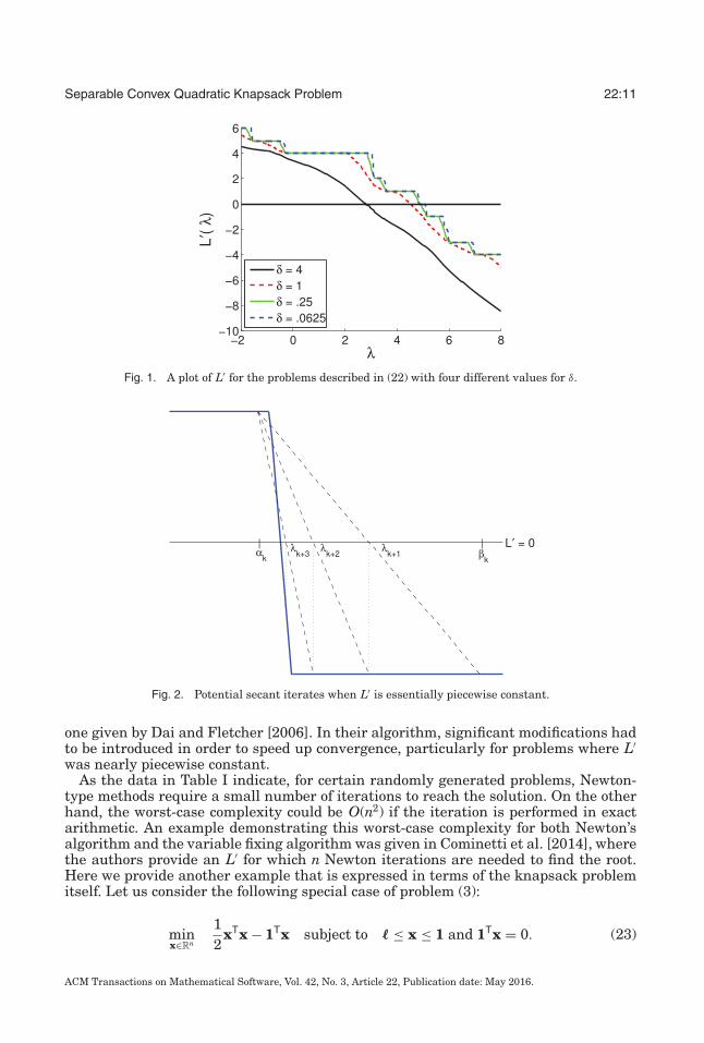
Here rand [−10, 10] denotes a random number between −10 and 10 with a uniformdistribution. The series of problems depends on the parameter δ. In Figure 1 we plotL′ for four different values of δ. When δ = 4, the plot is approximately linear, andNewton’s method should find the root quickly. However, when δ decreases to 1, the plotdevelops a flat spot, and any Newton iterate landing on this flat spot would be kickedout toward ±∞. When δ reaches 0.0625, the graph is essentially piecewise constant,and, in this case, Newton’s method would not work well.

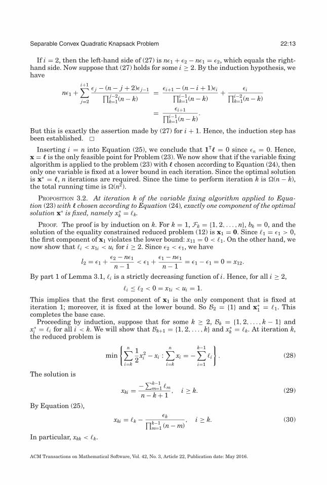
To correct for this poor performance, the authors of Cominetti et al. [2014] imple-ment a safeguard; whenever the Newton iterate lies outside the interval (αk−1, βk−1),the multiplier update is computed by either moving to the next break point in thedirection of λ∗ or using a secant step. In either case, convergence may be quite slow. Forexample, Figure 2 shows that when the graph of L′ is essentially piecewise constant,the convergence of a secant iteration based on the function values at αk−1 and βk−1 canbe slow. Similar difficulties may be encountered when using a secant method like the



Fig. 1. A plot of L′ for the problems described in (22) with four different values for δ.

Fig. 2. Potential secant iterates when L′ is essentially piecewise constant.

one given by Dai and Fletcher [2006]. In their algorithm, significant modifications hadto be introduced in order to speed up convergence, particularly for problems where L′was nearly piecewise constant.

As the data in Table I indicate, for certain randomly generated problems, Newton-type methods require a small number of iterations to reach the solution. On the otherhand, the worst-case complexity could be O(n2) if the iteration is performed in exactarithmetic. An example demonstrating this worst-case complexity for both Newton’salgorithm and the variable fixing algorithm was given in Cominetti et al. [2014], wherethe authors provide an L′ for which n Newton iterations are needed to find the root.Here we provide another example that is expressed in terms of the knapsack problemitself. Let us consider the following special case of problem (3):

minx∈Rn

12

xTx − 1Tx subject to � ≤ x ≤ 1 and 1Tx = 0. (23)



Consider any lower bound � of the following form:

�1 = ε1, �i = ε1 +i∑

j=2

ε j − (n − j + 2)ε j−1∏ j−1k=1(n − k)

for all i ≥ 2, (24)

where εi is an arbitrary sequence that satisfies 1 > ε1 > ε2 > · · · > εn = 0.

LEMMA 3.1. The components of � given in (24) satisfy the following:

(1) 1 > �1 > �2 > · · · > �n.(2) For each i ≥ 2, the following relation holds:

�i = −∑i−1m=1 �m

n − i + 1+ εi∏i−1

m=1 (n − m). (25)

PROOF.Part 1. Since the sequence εi is strictly decreasing and non-negative, it follows that,

for any 2 ≤ j ≤ n, we have

ε j − (n − j + 2)ε j−1 < ε j − ε j−1 < 0.

Hence, the terms in the sum in (24) are all negative, which implies that the sequence�i is strictly decreasing and �1 = ε1 < 1.

Part 2. Substituting �m using (24), we obtain

i−1∑m=1

�m = (i − 1)ε1 +i−1∑m=1

m∑j=2

ε j − (n − j + 2)ε j−1∏ j−1k=1(n − k)

. (26)

Notice that for each 2 ≤ j ≤ n, the term ε j−(n− j+2)ε j−1∏ j−1k=1(n−k)

appears exactly (i − j) times in

the sum of (26). Hence, Equation (26) simplifies to

i−1∑m=1

�m = (i − 1)ε1 +i−1∑j=2

(ε j − (n − j + 2)ε j−1∏ j−1

k=1(n − k)

)(i − j).

We make this substitution on the right-hand side of (25), the substitution (24) on theleft, and multiply by n − i + 1 to obtain

ε1(n − i + 1) +i∑

j=2

(ε j − (n − j + 2)ε j−1∏ j−1

k=1(n − k)

)(n − i + 1)

= −ε1(i − 1) −i−1∑j=2

ε j − (n − j + 2)ε j−1∏ j−1k=1(n − k)

(i − j) + εi∏i−2k=1(n − k)

.

In the special case i = 2, this relation remains valid if the products are treated as 1 andthe sums are treated as 0 when the lower limit exceeds the upper limit. We rearrangethis relation to get

nε1 +i∑

j=2

ε j − (n − j + 2)ε j−1∏ j−2k=1(n − k)

= εi∏i−2k=1(n − k)

. (27)

Hence, Equation (25) is equivalent to Equation (27). We prove Equation (27) byinduction.



If i = 2, then the left-hand side of (27) is nε1 + ε2 − nε1 = ε2, which equals the right-hand side. Now suppose that (27) holds for some i ≥ 2. By the induction hypothesis, wehave

nε1 +i+1∑j=2

ε j − (n − j + 2)ε j−1∏ j−2k=1(n − k)

= εi+1 − (n − i + 1)εi∏i−1k=1(n − k)

+ εi∏i−2k=1(n − k)

= εi+1∏i−1k=1(n − k)

.

But this is exactly the assertion made by (27) for i + 1. Hence, the induction step hasbeen established.

Inserting i = n into Equation (25), we conclude that 1T� = 0 since εn = 0. Hence,x = � is the only feasible point for Problem (23). We now show that if the variable fixingalgorithm is applied to the problem (23) with � chosen according to Equation (24), thenonly one variable is fixed at a lower bound in each iteration. Since the optimal solutionis x∗ = �, n iterations are required. Since the time to perform iteration k is (n − k),the total running time is (n2).

PROPOSITION 3.2. At iteration k of the variable fixing algorithm applied to Equa-tion (23) with � chosen according to Equation (24), exactly one component of the optimalsolution x∗ is fixed, namely x∗

k = �k.

PROOF. The proof is by induction on k. For k = 1, Fk = {1, 2, . . . , n}, bk = 0, and thesolution of the equality constrained reduced problem (12) is x1 = 0. Since �1 = ε1 > 0,the first component of x1 violates the lower bound: x11 = 0 < �1. On the other hand, wenow show that �i < x1i < ui for i ≥ 2. Since ε2 < ε1, we have

l2 = ε1 + ε2 − nε1

n − 1< ε1 + ε1 − nε1

n − 1= ε1 − ε1 = 0 = x12.

By part 1 of Lemma 3.1, �i is a strictly decreasing function of i. Hence, for all i ≥ 2,

�i ≤ �2 < 0 = x1i < ui = 1.

This implies that the first component of x1 is the only component that is fixed atiteration 1; moreover, it is fixed at the lower bound. So B2 = {1} and x∗

1 = �1. Thiscompletes the base case.

Proceeding by induction, suppose that for some k ≥ 2, Bk = {1, 2, . . . , k − 1} andx∗

i = �i for all i < k. We will show that Bk+1 = {1, 2, . . . , k} and x∗k = �k. At iteration k,

the reduced problem is

min

{n∑

i=k

12

x2i − xi :

n∑i=k

xi = −k−1∑i=1

�i

}. (28)

The solution is

xki = −∑k−1m=1 �m

n − k + 1, i ≥ k. (29)

By Equation (25),

xki = �k − εk∏k−1m=1 (n − m)

, i ≥ k. (30)

In particular, xkk < �k.



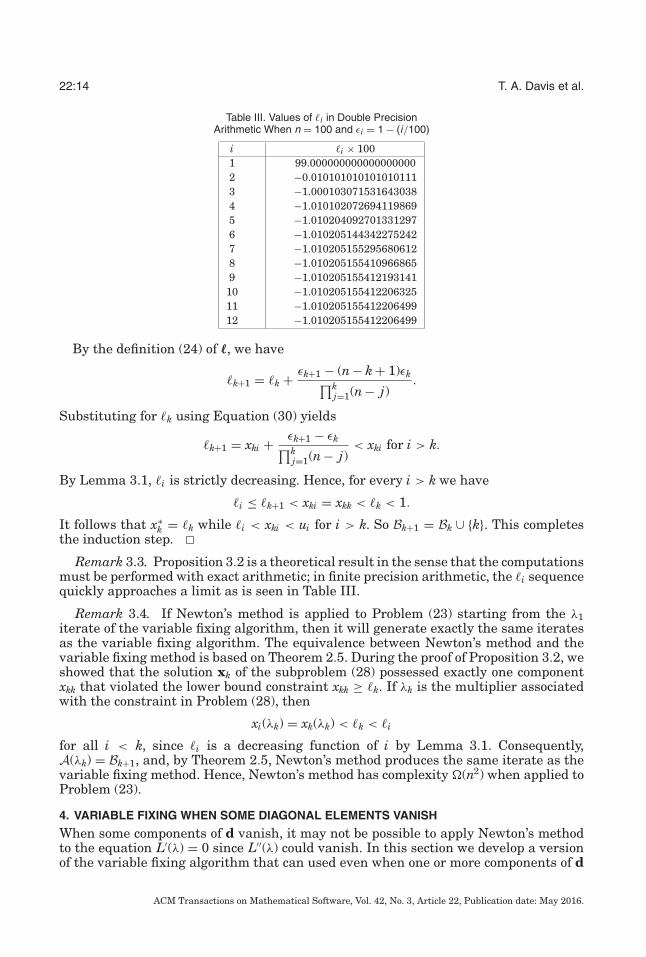
Table III. Values of �i in Double PrecisionArithmetic When n = 100 and εi = 1 − (i/100)

i �i × 1001 99.0000000000000000002 −0.0101010101010101113 −1.0001030715316430384 −1.0101020726941198695 −1.0102040927013312976 −1.0102051443422752427 −1.0102051552956806128 −1.0102051554109668659 −1.01020515541219314110 −1.01020515541220632511 −1.01020515541220649912 −1.010205155412206499

By the definition (24) of �, we have

�k+1 = �k + εk+1 − (n − k + 1)εk∏kj=1(n − j)

.

Substituting for �k using Equation (30) yields

�k+1 = xki + εk+1 − εk∏kj=1(n − j)

< xki for i > k.

By Lemma 3.1, �i is strictly decreasing. Hence, for every i > k we have

�i ≤ �k+1 < xki = xkk < �k < 1.

It follows that x∗k = �k while �i < xki < ui for i > k. So Bk+1 = Bk ∪ {k}. This completes

the induction step.

Remark 3.3. Proposition 3.2 is a theoretical result in the sense that the computationsmust be performed with exact arithmetic; in finite precision arithmetic, the �i sequencequickly approaches a limit as is seen in Table III.

Remark 3.4. If Newton’s method is applied to Problem (23) starting from the λ1iterate of the variable fixing algorithm, then it will generate exactly the same iteratesas the variable fixing algorithm. The equivalence between Newton’s method and thevariable fixing method is based on Theorem 2.5. During the proof of Proposition 3.2, weshowed that the solution xk of the subproblem (28) possessed exactly one componentxkk that violated the lower bound constraint xkk ≥ �k. If λk is the multiplier associatedwith the constraint in Problem (28), then

xi(λk) = xk(λk) < �k < �i

for all i < k, since �i is a decreasing function of i by Lemma 3.1. Consequently,A(λk) = Bk+1, and, by Theorem 2.5, Newton’s method produces the same iterate as thevariable fixing method. Hence, Newton’s method has complexity (n2) when applied toProblem (23).

4. VARIABLE FIXING WHEN SOME DIAGONAL ELEMENTS VANISH

When some components of d vanish, it may not be possible to apply Newton’s methodto the equation L′(λ) = 0 since L′′(λ) could vanish. In this section we develop a versionof the variable fixing algorithm that can used even when one or more components of d



vanish. Assuming L(λ) > −∞ (that is, λ lies in the domain of L), the set of minimizersX(λ) for the dual function (6) is

X(λ) = arg min{L(x, λ) : � ≤ x ≤ u}. (31)

If di > 0, then the ith component of X(λ) is unique and is given by (8). The associatedbreak points (9) are (yi − �idi)/ai and (yi − uidi)/ai. Between the break points, Xi(λ) =(yi − λai)/di, while outside the break point interval, Xi(λ) = �i or ui. If di = 0 and λ liesin the interior of the domain of the dual function, then

Xi(λ) = arg min {(λai − yi)xi : �i ≤ xi ≤ ui} ={

�i if aiλ > yi,

[�i, ui] if aiλ = yi,ui if aiλ < yi.

The interval [�i, ui] corresponds to the break point λ = yi/ai. On either side of the breakpoint, Xi(λ) equals either �i or ui. Hence, for any d ≥ 0, X(λ) is a linear function of λ onthe interior of any interval located between break points.

By Clarke [1975, Thm. 2.1] or Danskin [1967], the subdifferential of L can be ex-pressed

∂L(λ) = [L′(λ+), L′(λ−)], (32)

where

L′(λ+) = min{aTx − b : x ∈ X(λ)} and L′(λ−) = max{aTx − b : x ∈ X(λ)}.Since L is concave, its subdifferential is monotone; in particular, if λ1 < λ2, g1 ∈ ∂L(λ1),and g2 ∈ ∂L(λ2), then g1 ≥ g2. The generalization of Proposition 2.1 is the following:

PROPOSITION 4.1. If d ≥ 0 and there exists an optimal solution x∗ of (3), then thereexists a maximizer λ∗ of the dual function, 0 ∈ ∂L(λ∗), and x∗ ∈ X(λ∗). Moreover, anyx∗ ∈ X(λ∗) with aTx∗ = b is optimal in (3).

PROOF. The existence of a maximizer λ∗ of the dual function along with the optimalityconditions for λ∗ and x∗ are well-known properties of a concave optimization problem(see Luenberger and Ye [2008] and Rockafellar [1970]).

For any given λ and for all sufficiently small ε > 0, the sets X(λ + ε) and X(λ − ε) aresingletons. We define

X(λ+) := limε→0+

X(λ + ε) and X(λ−) := limε→0+

X(λ − ε).

The following proposition extends Proposition 2.2 to the case d ≥ 0:

PROPOSITION 4.2. If d ≥ 0, a > 0, and x∗ is optimal in (3), then for any λ in the domainof L, we have the following:

(1) If L′(λ+) ≥ 0, then x∗i = �i for every i such that Xi(λ+) = �i .

(2) If L′(λ−) ≤ 0, then x∗i = ui for every i such that Xi(λ−) = ui.

PROOF. Since the proofs of parts 1 and 2 are similar, we only prove part 1. Let λ∗ max-imize L. By Proposition 4.1, 0 ∈ ∂L(λ∗). If L′(λ+) ≥ 0, it follows from the monotonicityof ∂L, that λ ≤ λ∗.

Case 1. First suppose that λ = λ∗ and Xi(λ+) = �i. Since 0 ∈ ∂L(λ∗) =∂L(λ) =[L′(λ+), L′(λ−)], we conclude that L′(λ+) ≤ 0. By assumption, L′(λ+) ≥ 0. Soit follows that L′(λ+) = 0. If di > 0, then Xi(λ) = Xi(λ+) = �i. So since λ = λ∗, Xi(λ∗) = �i.And since x∗ ∈ X(λ∗) by Proposition 4.1, x∗

i = �i. If di = 0, then since Xi(λ+) = �i, itfollows that λai − yi = λ∗ai − yi ≥ 0. If λ∗ai − yi > 0, then x∗

i = Xi(λ∗) = �i. If λai − yi = 0,then Xi(λ) =Xi(λ∗) = [�i, ui]. Since x∗ is optimal in Problem (3), we have aTx∗ = b. If



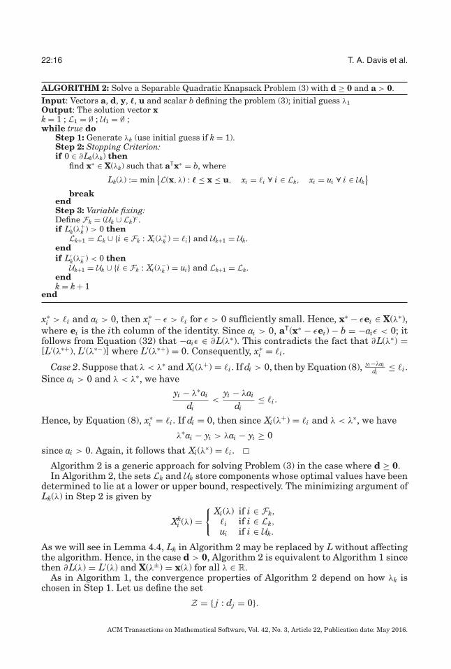
ALGORITHM 2: Solve a Separable Quadratic Knapsack Problem (3) with d ≥ 0 and a > 0.Input: Vectors a, d, y, �, u and scalar b defining the problem (3); initial guess λ1Output: The solution vector xk = 1 ; L1 = ∅ ; U1 = ∅ ;while true do

Step 1: Generate λk (use initial guess if k = 1).Step 2: Stopping Criterion:if 0 ∈ ∂Lk(λk) then

find x∗ ∈ X(λk) such that aTx∗ = b, where

Lk(λ) := min{L(x, λ) : � ≤ x ≤ u, xi = �i ∀ i ∈ Lk, xi = ui ∀ i ∈ Uk

}break

endStep 3: Variable fixing:Define Fk = (Uk ∪ Lk)c.if L′

k(λ+k ) > 0 then

Lk+1 = Lk ∪ {i ∈ Fk : Xi(λ+k ) = �i} and Uk+1 = Uk.

endif L′

k(λ−k ) < 0 then

Uk+1 = Uk ∪ {i ∈ Fk : Xi(λ−k ) = ui} and Lk+1 = Lk.

endk = k + 1

end

x∗i > �i and ai > 0, then x∗

i − ε > �i for ε > 0 sufficiently small. Hence, x∗ − εei ∈ X(λ∗),where ei is the ith column of the identity. Since ai > 0, aT(x∗ − εei) − b = −aiε < 0; itfollows from Equation (32) that −aiε ∈ ∂L(λ∗). This contradicts the fact that ∂L(λ∗) =[L′(λ∗+), L′(λ∗−)] where L′(λ∗+) = 0. Consequently, x∗

i = �i.

Case 2. Suppose that λ < λ∗ and Xi(λ+) = �i. If di > 0, then by Equation (8), yi−λaidi

≤ �i.Since ai > 0 and λ < λ∗, we have

yi − λ∗ai

di<

yi − λai

di≤ �i.

Hence, by Equation (8), x∗i = �i. If di = 0, then since Xi(λ+) = �i and λ < λ∗, we have

λ∗ai − yi > λai − yi ≥ 0

since ai > 0. Again, it follows that Xi(λ∗) = �i.

Algorithm 2 is a generic approach for solving Problem (3) in the case where d ≥ 0.In Algorithm 2, the sets Lk and Uk store components whose optimal values have been

determined to lie at a lower or upper bound, respectively. The minimizing argument ofLk(λ) in Step 2 is given by

Xki (λ) =

{ Xi(λ) if i ∈ Fk,�i if i ∈ Lk,ui if i ∈ Uk.

As we will see in Lemma 4.4, Lk in Algorithm 2 may be replaced by L without affectingthe algorithm. Hence, in the case d > 0, Algorithm 2 is equivalent to Algorithm 1 sincethen ∂L(λ) = L′(λ) and X(λ±) = x(λ) for all λ ∈ R.

As in Algorithm 1, the convergence properties of Algorithm 2 depend on how λk ischosen in Step 1. Let us define the set

Z = { j : dj = 0}.



When Z �= ∅, the variable fixing iterates λFk defined in (14) and the Newton iterates

(15) may be invalid, due to division by zero. However, the variable fixing algorithm hasa natural extension to the case Z �= ∅, as we will now show.

Given an instance of Problem (3) with d ≥ 0, let ε > 0 and define dε by

dεi =

{ε if i ∈ Z,di if i /∈ Z,

i = 1, 2, . . . , n. Consider the perturbed problem

minx∈Rn

{12

xTDεx − yTx : � ≤ x ≤ u, aTx = b}

, (33)

where Dε is the diagonal matrix with dε on the diagonal. Since dεi > 0 for every i, the

kth variable fixing iterate for (33) is well defined and is given by

λFk,ε =

−bk + ∑i∈Fk\Z

yiaidi

+ ∑i∈Fk∩Z

yiaiε∑

i∈Fk\Za2

idi

+ ∑i∈Fk∩Z

a2iε

=−εbk + ε

∑i∈Fk\Z

yiaidi

+ ∑i∈Fk∩Z yiai

ε∑

i∈Fk\Za2

idi

+ ∑i∈Fk∩Z a2

i

.

Hence when Z ∩ Fk �= ∅, we have

λFk,0 := lim

ε→0+λF

k,ε =∑

i∈Z∩Fkyiai∑

i∈Z∩Fka2

i

.

This motivates the following theorem.

THEOREM 4.3. Let d ≥ 0, a > 0, and suppose that (3) has an optimal solution. Foreach iteration k ≥ 1 of Algorithm 2, let λk be defined by

λk ={

λFk,0 if Z ∩ Fk �= ∅,

λFk if Z ∩ Fk = ∅.

(34)

Then Algorithm 2 converges in finitely many iterations to some λ∗ such that 0 ∈ ∂L(λ∗).Hence, any x∗ ∈ X(λ∗) such that aTx∗ = b is optimal in Problem (3).

The proof of Theorem 4.3 is based on the following lemma.

LEMMA 4.4. Let d ≥ 0, a > 0, and suppose that Problem (3) has an optimal solution.For each iteration k ≥ 1, define

λLk := sup{λi : 1 ≤ i ≤ k − 1, L′

i(λ+i ) > 0},

λRk := inf{λi : 1 ≤ i ≤ k − 1, L′

i(λ−i ) < 0},

where sup ∅ := −∞ and inf ∅ := ∞. Then, for every k ≥ 1 such that Z ∩ Fk �= ∅, thefollowing hold:

(1) λk ∈ (λLk , λR

k ).(2) If 0 /∈ ∂Lk(λk), then either |Lk+1| > |Lk| or |Uk+1| > |Uk|.(3) Lk(λ) = L(λ) for every λ ∈ (λL

k , λRk ).

(4) For every λ ∈ R with 0 ∈ ∂Lk(λ), we have 0 ∈ ∂L(λ).



PROOF. Parts 1 and 2: Since Z ∩ Fk �= ∅, we have

λk =∑

i∈Z∩Fkyiai∑

j∈Z∩Fka2

j

=∑

i∈Z∩Fk

yi

ai

(a2

i∑j∈Z∩Fk

a2j

)=

∑i∈Z∩Fk

αi,k

(yi

ai

),

where αi,k = a2i∑

j∈Z∩Fka2

j> 0 and

∑i∈Z∩Fk

αi,k = 1. Hence, λk is a convex combination of

breakpoints associated with components in Z∩Fk. In particular, there exist i, j ∈ Z∩Fksuch that

yi

ai≤ λk ≤ yj

aj. (35)

Next, we claim that λLk <

yiai

. Indeed, suppose by way of contradiction that this is nottrue. Then, by definition of λL

k , there is some (smallest) l ≤ k − 1 such that L′l(λ

+l ) > 0

and λl ≥ yiai

. Since λl ≥ yiai

, Xi(λ+l ) = �i by definition of X, and on Step 3 of the lth

iteration of Algorithm 2, i ∈ Ll+1\Ll ⊆ Lk, contradicting i ∈ Fk. By a similar argument,yj

aj< λR

k . Hence, by Equation (35) λLk < λk < λR

k , which proves Part 1.Now, suppose that 0 /∈ ∂Lk(λk). Then by Equation (32) either L′

k(λ+k ) > 0 or L′

k(λ−k ) < 0.

Notice that (35) implies that Xi(λ+k ) = �i and Xj(λ−

k ) = uj , by definition of X. Hence,if L′

k(λ+k ) > 0, then by Step 3 of the kth iteration of Algorithm 2 we have i ∈ Lk+1\Lk;

whereas if L′k(λ−

k ) < 0, then j ∈ Uk+1\Uk. This completes the proof of Part 2.Parts 3 and 4: We prove Parts 3 and 4 by induction on k. The base cases where

k = 1 are trivial, since L1 = L. So, suppose that for some s ≥ 1, we have Z ∩ Fk �= ∅and Parts 3 and 4 hold for every k ≤ s. Suppose that Z ∩ Fs+1 �= ∅. We will show thatParts 3 and 4 hold for k = s + 1.

Since the algorithm did not stop on iteration s, we must have 0 /∈ ∂Ls(λs). We assumewithout loss of generality that L′

s(λ+s ) > 0 (the proof in the case L′

s(λ−s ) < 0 is similar).

By the induction hypothesis, Ls(λ) = L(λ) for any λ ∈ (λLs , λR

s ) ⊇ (λLs+1, λ

Rs+1). Hence, we

will be done with Part 3 when we show that Ls+1(λ) = Ls(λ) for every λ ∈ (λLs+1, λ

Rs+1).

Let λ ∈ (λLs+1, λ

Rs+1). Since L′

s(λ+s ) > 0 by assumption, Step 3 of the algorithm gives

Us+1 = Us and Ls ⊂ Ls+1. Hence, Xs+1i (λ) = Xs

i (λ) = ui for all i ∈ Us+1 and Xs+1i (λ) =

Xsi (λ) = �i for all i ∈ Ls. Since F s+1 ⊂ F s, it follows that Xs+1

i (λ) = Xsi (λ) for all

i ∈ Fs+1. Hence, the only indices where Xs+1i (λ) Xs

i (λ) could differ are those i ∈ Ls+1\Ls.We will now show that for every i ∈ Ls+1\Ls, Xs

i (λ) = �i = Xs+1i (λ). This will imply

Xs+1(λ) = Xs(λ), and therefore Ls+1(λ) = Ls(λ).Let i ∈ Ls+1\Ls. Since L′

s(λ+s ) > 0 by assumption, Step 3 of the algorithm implies

Xi(λ+s ) = �i. (36)

By Part 1, λs ∈ (λLs , λR

s ); hence by definition of λLs+1,

λLs+1 = λs. (37)

Since λ > λLs+1 = λs and Xi(·) is nonincreasing and bounded below by �i, we have

Xi(λ) = �i. Thus, Xsi (λ) = Xi(λ) = �i = Xs+1

i (λ).Since i ∈ Ls+1\Ls was arbitrary, we have shown that Xs+1(λ) = Xs(λ); hence, Ls+1(λ) =

Ls(λ). Since λ ∈ (λLs+1, λ

Rs+1) was arbitrary, we have shown that

Ls+1(λ) = Ls(λ) = L(λ) ∀ λ ∈ (λL

s+1, λRs+1

), (38)

which proves Part 3 for k = s + 1.



Now we prove Part 4 holds for k = s + 1. Suppose that 0 ∈ ∂Ls+1(λ) for some λ ∈ R.Then by Equation (32),

L′s+1(λ+) ≤ 0 ≤ L′

s+1(λ−). (39)

We claim that λ ∈ (λLs+1, λ

Rs+1). Once this claim is proved, it will follow from Equation

(38) that ∂L(λ) = ∂Ls+1(λ). Since 0 ∈ ∂Ls+1(λ), we will have 0 ∈ ∂L(λ), and the proof willbe complete.

First, we show λLs+1 < λ. If λL

s+1 = −∞, then we are done. So, suppose λLs+1 > −∞.

ThenL′

s+1

(λL+

s+1

) = L′s

(λL+

s+1

) = L′s

(λ+

s

)> 0, (40)

where the first equality follows from Equation (38), the second follows from Equa-tion (37), and the inequality follows from our assumption. Since ∂Ls+1(·) is monotonenonincreasing, Equation (40) and the first half of Equation (39) imply λL

s+1 < λ.Now, we show λ < λR

s+1. If λRs+1 = ∞, then we are done. So, suppose λR

s+1 < ∞. ThenλR

s+1 = λ j for some j ≤ s such that L′j(λ

−j ) < 0. By Equation (38) and the induction

assumption for Part 3,

Ls+1(λ) = L(λ) = Lj(λ) ∀ λ ∈ (λL

s+1, λRs+1

) ⊆ (λL

j , λRj

).

Hence,

L′s+1

(λR−

s+1

) = L′j

(λR−

s+1

) = L′j

(λ−

j

)< 0. (41)

So, since ∂L(·) is monotone nonincreasing, Equation (41) and the second half of Equa-tion (39) imply λ < λR

s+1. Thus, λ ∈ (λLs+1, λ

Rs+1), and our claim is proved. This completes

the proof of Part 4 for k = s + 1.Therefore, the proof of Parts 3 and 4 is complete by induction.

Remark 4.5. By Lemma 4.4, we may replace Lk with L in Algorithm 2. Hence, in thecase where Z = ∅, Algorithm 2 is equivalent to Algorithm 1, since then ∂L(λ) = L′(λ)and X(λ±) = x(λ) for all λ ∈ R.

PROOF OF THEOREM 4.3. By Part 2 of Lemma 4.4, since |Lk| and |Uk| are bounded fromabove by n, we eventually must reach an iteration s ≥ 1 such that either

[Z ∩ Fs = ∅] or [Z ∩ Fs �= ∅ and 0 ∈ ∂Ls(λs)]. (42)

Let s be the first iteration satisfying Equation (42). In the second case of Equation (42),we have 0 ∈ ∂L(λs) by Part 3 of Lemma 4.4, and we are done. Now suppose instead thatthe first case holds. Then for k ≥ s, λk = λF

k and Algorithm 2 reduces to the VariableFixing Algorithm of Kiwiel [2008] for the problem

min q(x)subject to � ≤ x ≤ u, aTx = b, xi = �i ∀ i ∈ Ls, and xi = ui ∀ i ∈ Us.

(The formula for λFk (14) comes directly from Kiwiel [2008, page 448]). Therefore, by

Kiwiel [2008, Theorem 4.1], λk converges to some λ∗ such that

∂Ls(λ∗) = L′s(λ

∗) = aTs xs(λ∗) − bs = 0,

where as and xs(λ∗) represent the vectors formed by only including components in Fs,and bs is defined by

bs = b −∑i∈Ls

ai�i −∑i∈Us

aiui. (43)

Therefore, by Part 4 of Lemma 4.4, 0 ∈ ∂L(λ∗). This completes the proof.



5. NAPHEAP

In many problems, the iterates in a variable fixing method or Newton method exhibita diminishing returns property: Most of the progress towards finding the optimalmultiplier is made in the first several iterations, while subsequent iterations yieldsteps that are much smaller. We propose an algorithm called NAPHEAP that exploitsthis property. The algorithm first generates an interval (α, β) (possibly semi-infinite)that brackets a solution of the dual problem (7) by applying a few iterations of aNewton-type method. Then all the break points of the dual function between α and βare arranged in heaps. NAPHEAP then starts from either α or β and monotonicallyvisits the break points until reaching an optimal dual solution λ∗. Since L′ is linearon any interval between break points, a solution of the dual problem can be evaluatedby linear interpolation. If there are m break points in (α, β), then the time to updatethe heap after visiting a break point is proportional to log2 m. Similarly, the time tobuild a heap with m elements is roughly the time to perform m comparisons. Hence,when l break points are visited on the path to the solution, the total running time ofthe heap phase is proportional to m+ l log2 m. For details concerning the constructionand updating of heaps, see Cormen et al. [2009]. The steps of the NAPHEAP code arepartitioned into three phases that we now discuss in more detail.

NAPHEAP Phase 0. If ai = 0 for some i, then the optimal value for xi can evaluated,and xi can be eliminated from the problem. Hence, without loss of generality, we assumethat ai �= 0 for all i. If di = 0 for some i, then we evaluate the expressions

α0 = max{

yi

ai: di = 0 and ui = ∞

}and β0 = min

{yi

ai: di = 0 and �i = −∞

},

where the maximum and the minimum are defined to be ∞ and −∞, respectively, whenthe arguments are empty. L is finite on the interval [α0, β0], the domain of the dualfunction, and an optimal dual solution λ∗ lies between α0 and β0. If a starting guess λ1was not provided, then we evaluate one by performing a single iteration of the variablefixing algorithm. From the sign of L′(λ1), and the values of α0 and β0, we can furtherrefine the bracketing interval (α, β).

NAPHEAP Phase 1. The bracketing interval generated in phase 0 is further refinedby performing a few iterations of a Newton-type method. The optimal number of it-erations depends on the problem. When di = 0 for some i, Version 2.1 of NAPHEAPcurrently performs K (a user specified number) Newton-type iterations before switch-ing to the break point search. However, when d > 0, an adaptive strategy is employedbased on the following observation: Newton’s method often converges monotonically tothe solution of the dual problem. Hence, if we multiply the Newton step by a scalingfactor ξ > 1 (default 1.1), then the scaled Newton iterate

λk+1 = λk − ξ

(L′(λk)L′′±(λk)

)will typically lie on the opposite side of the root from λk when λk is sufficiently close to asolution. We continue to perform a scaled Newton iteration until we reach the oppositeside of the root, and then we terminate phase 1. When the scaled Newton iteratelands outside the current bracketing interval, then we attempt a secant iteration. Ifthe bracketing interval is semi-infinite and the secant iteration cannot be performed,then we use a variable fixing iteration. We impose an upper bound on the number ofNewton-type iterations (default (20)).

NAPHEAP Phase 2. Phase 1 generates either the solution of the knapsack problem oran interval [α, β] (possibly semi-infinite) that brackets a solution of the dual problem;



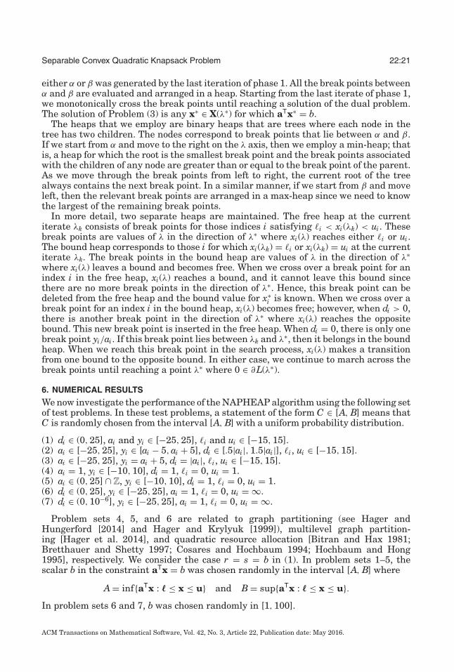
either α or β was generated by the last iteration of phase 1. All the break points betweenα and β are evaluated and arranged in a heap. Starting from the last iterate of phase 1,we monotonically cross the break points until reaching a solution of the dual problem.The solution of Problem (3) is any x∗ ∈ X(λ∗) for which aTx∗ = b.

The heaps that we employ are binary heaps that are trees where each node in thetree has two children. The nodes correspond to break points that lie between α and β.If we start from α and move to the right on the λ axis, then we employ a min-heap; thatis, a heap for which the root is the smallest break point and the break points associatedwith the children of any node are greater than or equal to the break point of the parent.As we move through the break points from left to right, the current root of the treealways contains the next break point. In a similar manner, if we start from β and moveleft, then the relevant break points are arranged in a max-heap since we need to knowthe largest of the remaining break points.

In more detail, two separate heaps are maintained. The free heap at the currentiterate λk consists of break points for those indices i satisfying �i < xi(λk) < ui. Thesebreak points are values of λ in the direction of λ∗ where xi(λ) reaches either �i or ui.The bound heap corresponds to those i for which xi(λk) = �i or xi(λk) = ui at the currentiterate λk. The break points in the bound heap are values of λ in the direction of λ∗where xi(λ) leaves a bound and becomes free. When we cross over a break point for anindex i in the free heap, xi(λ) reaches a bound, and it cannot leave this bound sincethere are no more break points in the direction of λ∗. Hence, this break point can bedeleted from the free heap and the bound value for x∗

i is known. When we cross over abreak point for an index i in the bound heap, xi(λ) becomes free; however, when di > 0,there is another break point in the direction of λ∗ where xi(λ) reaches the oppositebound. This new break point is inserted in the free heap. When di = 0, there is only onebreak point yi/ai. If this break point lies between λk and λ∗, then it belongs in the boundheap. When we reach this break point in the search process, xi(λ) makes a transitionfrom one bound to the opposite bound. In either case, we continue to march across thebreak points until reaching a point λ∗ where 0 ∈ ∂L(λ∗).

6. NUMERICAL RESULTS

We now investigate the performance of the NAPHEAP algorithm using the following setof test problems. In these test problems, a statement of the form C ∈ [A, B] means thatC is randomly chosen from the interval [A, B] with a uniform probability distribution.

(1) di ∈ (0, 25], ai and yi ∈ [−25, 25], �i and ui ∈ [−15, 15].(2) ai ∈ [−25, 25], yi ∈ [ai − 5, ai + 5], di ∈ [.5|ai|, 1.5|ai|], �i, ui ∈ [−15, 15].(3) ai ∈ [−25, 25], yi = ai + 5, di = |ai|, �i, ui ∈ [−15, 15].(4) ai = 1, yi ∈ [−10, 10], di = 1, �i = 0, ui = 1.(5) ai ∈ (0, 25] ∩ Z, yi ∈ [−10, 10], di = 1, �i = 0, ui = 1.(6) di ∈ (0, 25], yi ∈ [−25, 25], ai = 1, �i = 0, ui = ∞.(7) di ∈ (0, 10−6], yi ∈ [−25, 25], ai = 1, �i = 0, ui = ∞.

Problem sets 4, 5, and 6 are related to graph partitioning (see Hager andHungerford [2014] and Hager and Krylyuk [1999]), multilevel graph partition-ing [Hager et al. 2014], and quadratic resource allocation [Bitran and Hax 1981;Bretthauer and Shetty 1997; Cosares and Hochbaum 1994; Hochbaum and Hong1995], respectively. We consider the case r = s = b in (1). In problem sets 1–5, thescalar b in the constraint aTx = b was chosen randomly in the interval [A, B] where

A = inf{aTx : � ≤ x ≤ u} and B = sup{aTx : � ≤ x ≤ u}.In problem sets 6 and 7, b was chosen randomly in [1, 100].



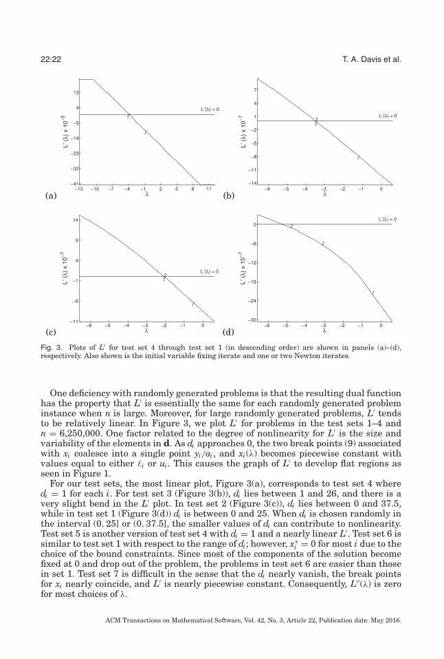
Fig. 3. Plots of L′ for test set 4 through test set 1 (in descending order) are shown in panels (a)–(d),respectively. Also shown is the initial variable fixing iterate and one or two Newton iterates.

One deficiency with randomly generated problems is that the resulting dual functionhas the property that L′ is essentially the same for each randomly generated probleminstance when n is large. Moreover, for large randomly generated problems, L′ tendsto be relatively linear. In Figure 3, we plot L′ for problems in the test sets 1–4 andn = 6,250,000. One factor related to the degree of nonlinearity for L′ is the size andvariability of the elements in d. As di approaches 0, the two break points (9) associatedwith xi coalesce into a single point yi/ai, and xi(λ) becomes piecewise constant withvalues equal to either �i or ui. This causes the graph of L′ to develop flat regions asseen in Figure 1.

For our test sets, the most linear plot, Figure 3(a), corresponds to test set 4 wheredi = 1 for each i. For test set 3 (Figure 3(b)), di lies between 1 and 26, and there is avery slight bend in the L′ plot. In test set 2 (Figure 3(c)), di lies between 0 and 37.5,while in test set 1 (Figure 3(d)) di is between 0 and 25. When di is chosen randomly inthe interval (0, 25] or (0, 37.5], the smaller values of di can contribute to nonlinearity.Test set 5 is another version of test set 4 with di = 1 and a nearly linear L′. Test set 6 issimilar to test set 1 with respect to the range of di; however, x∗

i = 0 for most i due to thechoice of the bound constraints. Since most of the components of the solution becomefixed at 0 and drop out of the problem, the problems in test set 6 are easier than thosein set 1. Test set 7 is difficult in the sense that the di nearly vanish, the break pointsfor xi nearly coincide, and L′ is nearly piecewise constant. Consequently, L′′(λ) is zerofor most choices of λ.



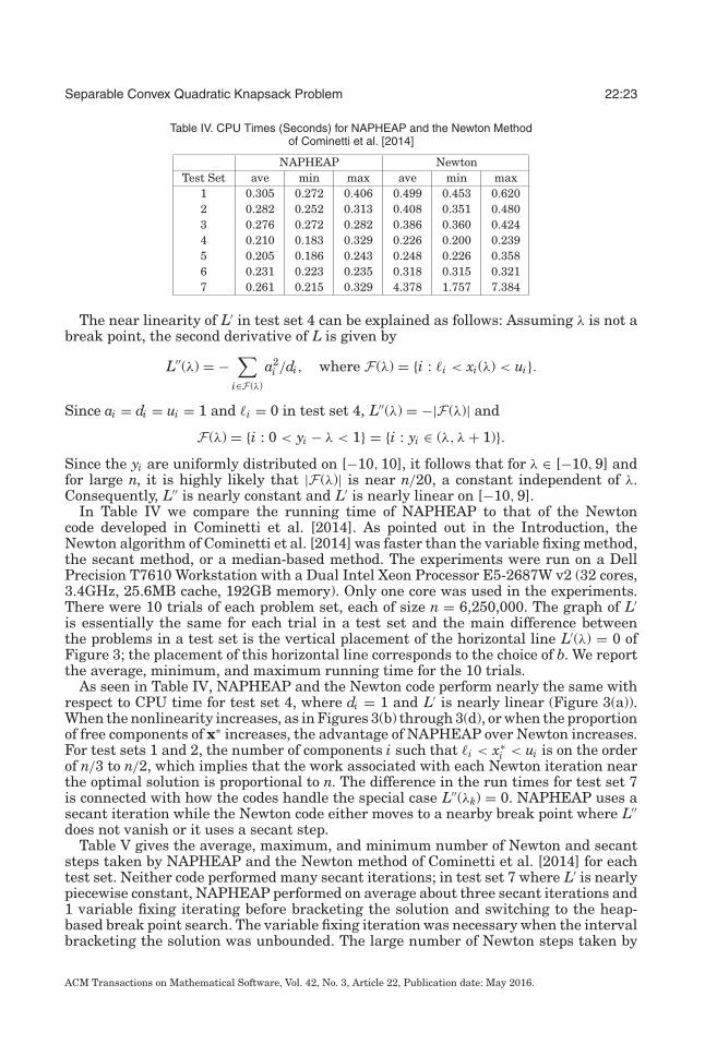
Table IV. CPU Times (Seconds) for NAPHEAP and the Newton Methodof Cominetti et al. [2014]

NAPHEAP NewtonTest Set ave min max ave min max

1 0.305 0.272 0.406 0.499 0.453 0.6202 0.282 0.252 0.313 0.408 0.351 0.4803 0.276 0.272 0.282 0.386 0.360 0.4244 0.210 0.183 0.329 0.226 0.200 0.2395 0.205 0.186 0.243 0.248 0.226 0.3586 0.231 0.223 0.235 0.318 0.315 0.3217 0.261 0.215 0.329 4.378 1.757 7.384

The near linearity of L′ in test set 4 can be explained as follows: Assuming λ is not abreak point, the second derivative of L is given by

L′′(λ) = −∑

i∈F(λ)

a2i /di, where F(λ) = {i : �i < xi(λ) < ui}.

Since ai = di = ui = 1 and �i = 0 in test set 4, L′′(λ) = −|F(λ)| and

F(λ) = {i : 0 < yi − λ < 1} = {i : yi ∈ (λ, λ + 1)}.Since the yi are uniformly distributed on [−10, 10], it follows that for λ ∈ [−10, 9] andfor large n, it is highly likely that |F(λ)| is near n/20, a constant independent of λ.Consequently, L′′ is nearly constant and L′ is nearly linear on [−10, 9].

In Table IV we compare the running time of NAPHEAP to that of the Newtoncode developed in Cominetti et al. [2014]. As pointed out in the Introduction, theNewton algorithm of Cominetti et al. [2014] was faster than the variable fixing method,the secant method, or a median-based method. The experiments were run on a DellPrecision T7610 Workstation with a Dual Intel Xeon Processor E5-2687W v2 (32 cores,3.4GHz, 25.6MB cache, 192GB memory). Only one core was used in the experiments.There were 10 trials of each problem set, each of size n = 6,250,000. The graph of L′is essentially the same for each trial in a test set and the main difference betweenthe problems in a test set is the vertical placement of the horizontal line L′(λ) = 0 ofFigure 3; the placement of this horizontal line corresponds to the choice of b. We reportthe average, minimum, and maximum running time for the 10 trials.

As seen in Table IV, NAPHEAP and the Newton code perform nearly the same withrespect to CPU time for test set 4, where di = 1 and L′ is nearly linear (Figure 3(a)).When the nonlinearity increases, as in Figures 3(b) through 3(d), or when the proportionof free components of x∗ increases, the advantage of NAPHEAP over Newton increases.For test sets 1 and 2, the number of components i such that �i < x∗

i < ui is on the orderof n/3 to n/2, which implies that the work associated with each Newton iteration nearthe optimal solution is proportional to n. The difference in the run times for test set 7is connected with how the codes handle the special case L′′(λk) = 0. NAPHEAP uses asecant iteration while the Newton code either moves to a nearby break point where L′′does not vanish or it uses a secant step.

Table V gives the average, maximum, and minimum number of Newton and secantsteps taken by NAPHEAP and the Newton method of Cominetti et al. [2014] for eachtest set. Neither code performed many secant iterations; in test set 7 where L′ is nearlypiecewise constant, NAPHEAP performed on average about three secant iterations and1 variable fixing iterating before bracketing the solution and switching to the heap-based break point search. The variable fixing iteration was necessary when the intervalbracketing the solution was unbounded. The large number of Newton steps taken by



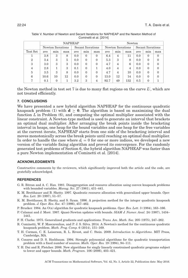
Table V. Number of Newton and Secant Iterations for NAPHEAP and the Newton Method ofCominetti et al. [2014]

NAPHEAP NewtonNewton Iterations Secant Iterations Newton Iterations Secant Iterations

Test Set ave min max ave min max ave min max ave min max1 3.8 3 8 0.0 0 0 6.4 4 11 0.0 0 02 3.4 3 5 0.0 0 0 5.3 3 8 0.0 0 03 3.0 3 3 0.0 0 0 4.7 4 6 0.0 0 04 2.8 1 3 0.1 0 1 4.0 4 4 0.0 0 05 3.5 3 8 0.0 0 0 4.7 4 10 0.0 0 06 10.6 10 12 0.0 0 0 13.0 12 14 0.0 0 07 0.1 0 1 3.2 3 4 92.7 49 132 0.5 0 1

the Newton method in test set 7 is due to many flat regions on the curve L′, which arenot treated efficiently.

7. CONCLUSIONS

We have presented a new hybrid algorithm NAPHEAP for the continuous quadraticknapsack problem (1) with d ≥ 0. The algorithm is based on maximizing the dualfunction L in Problem (6), and computing the optimal multiplier associated with thelinear constraint. A Newton-type method is used to generate an interval that bracketsan optimal dual multiplier. After arranging the break points inside the bracketinginterval in heaps, one heap for the bound variables and one heap for the free variablesat the current iterate, NAPHEAP starts from one side of the bracketing interval andmoves monotonically across the break points until reaching an optimal dual multiplier.In order to handle the case where di = 0 for one or more indices, we developed a newversion of the variable fixing algorithm and proved its convergence. For the randomlygenerated test problems of Section 6, the hybrid algorithm NAPHEAP was faster thana pure Newton implementation of Cominetti et al. [2014].

ACKNOWLEDGMENTS

Constructive comments by the reviewers, which significantly improved both the article and the code, aregratefully acknowledged.

REFERENCES

G. R. Bitran and A. C. Hax. 1981. Disaggregation and resource allocation using convex knapsack problemswith bounded variables. Manag. Sci. 27 (1981), 431–441.

K. M. Bretthauer and B. Shetty. 1997. Quadratic resource allocation with generalized upper bounds. Oper.Res. Lett. 20 (1997), 51–57.

K. M. Bretthauer, B. Shetty, and S. Syam. 1996. A projection method for the integer quadratic knapsackproblem. J. Oper. Res. Soc. 47 (1996), 457–462.

P. Brucker. 1984. An O(n) algorithm for quadratic knapsack problems. Oper. Res. Lett. 3 (1984), 163–166.P. Calamai and J. More. 1987. Quasi-Newton updates with bounds. SIAM J. Numer. Anal. 24 (1987), 1434–

1441.F. H. Clarke. 1975. Generalized gradients and applications. Trans. Am. Math. Soc. 205 (1975), 247–262.R. Cominetti, W. F. Mascarenhas, and P. J. S. Silva. 2014. A Newton’s method for the continuous quadratic

knapsack problem. Math. Prog. Comp. 6 (2014), 151–169.T. H. Cormen, C. E. Leiserson, R. L. Rivest, and C. Stein. 2009. Introduction to Algorithms. MIT Press,

Cambridge, MA.S. Cosares and D. S. Hochbaum. 1994. Strongly polynomial algorithms for the quadratic transportation

problem with a fixed number of sources. Math. Oper. Res. 19 (1994), 94–111.Y. H. Dai and R. Fletcher. 2006. New algorithms for singly linearly constrained quadratic programs subject

to lower and upper bounds. Math. Program. 106 (2006), 403–421.



J. M. Danskin. 1967. The Theory of Max-Min and its Applications to Weapons Allocation Problems. Springer-Verlag, New York, NY.

Y. S. Fu and Y. H. Dai. 2010. Improved projected gradient algorithms for singly linearly constrainedquadrataic programs subject to lower and upper bounds. Asia-Pac. J. Oper. Res. 27 (2010), 71–84.

W. W. Hager and J. T. Hungerford. 2014. Optimality conditions for maximizing a function over a polyhedron.Math. Program. 145 (2014), 179–198.

W. W. Hager and J. T. Hungerford. 2015. Continuous quadratic programming formulations of optimizationproblems on graphs. Eur. J. Oper. Res. 240 (2015), 328–337.

W. W. Hager, J. T. Hungerford, and I. Safro. 2014. A multilevel bilinear programming algorithm for the vertexseparator problem. http://clas.ufl.edu/users/hager/papers/GP/ml.pdf.

W. W. Hager and Y. Krylyuk. 1999. Graph partitioning and continuous quadratic programming. SIAM J.Disc. Math. 12 (1999), 500–523.

W. W. Hager and H. Zhang. 2006. A new active set algorithm for box constrained optimization. SIAM J.Optim. 17 (2006), 526–557.

K. Helgason, J. Kennington, and H. Lall. 1980. A polynomially bounded algorithm for a singly-constrainedquadratic program. Math. Program. 18 (1980), 338–343.

D. S. Hochbaum and S. P. Hong. 1995. About strongly polynomial time algorithms for quadratic optimizationover submodular constraints. Math. Program. 69 (1995), 269–309.

K. C. Kiwiel. 2008. Variable fixing algorithms for the continuous quadratic knapsack problem. J. Optim.Theory Appl. 136 (2008), 445–458.

D. G. Luenberger and Y. Ye. 2008. Linear and Nonlinear Programming. Springer, Berlin.N. Maculan, C. P. Santiago, E. M. Macambira, and M. H. C. Jardim. 2003. An O(n) algorithm for projecting a

vector on the intersection of a hyperplane and a box in Rn. J. Optim. Theory Appl. 117 (2003), 553–574.

C. Michelot. 1986. A finite algorithm for finding the projection of a point onto the canonical simplex of Rn. J.

Optim. Theory Appl. 50 (1986), 195–200.S. S. Nielsen and S. A. Zenios. 1992. Massively parallel algorithms for singly-constrained convex programs.

ORSA J. Comput. 4 (1992), 166–181.P. M. Pardalos and N. Kovoor. 1990. An algorithm for a singly constrained class of quadratic programs subject

to upper and lower bounds. Math. Program. 46 (1990), 321–328.A. G. Robinson, N. Jiang, and C. S. Lerme. 1992. On the continuous quadratic knapsack problem. Math.

Program. 55 (1992), 99–108.R. T. Rockafellar. 1970. Convex Analysis. Princeton University Press, Princeton, NJ.B. Shetty and R. Muthukrishnan. 1990. A parallel projection for the multicommodity network model. J. Oper.

Res. Soc. 41 (1990), 837–842.N. Z. Shor. 1985. Minimization Methods for Nondifferentiable Functions. Springer-Verlag, New York, NY.J. A. Ventura. 1991. Computational development of a Lagrangian dual approach for quadratic networks.

Networks 21 (1991), 469–485.

Received October 2013; revised September 2015; accepted September 2015


http://clas.ufl.edu/users/hager/papers/GP/ml.pdf

An Efﬁcient Hybrid Algorithm for the Separable Convex ...users.clas.ufl.edu/hager/papers/CG/knapsack.pdf · Additional Key Words and Phrases: Continuous quadratic knapsack, nonlinear

Documents