An Efﬁcient Adaptive Sequential Methodology for …users.iems.northwestern.edu/~bea/articles/An Efficient...An Efﬁcient Adaptive Sequential Methodology for Expensive Response Surface

Research Article

(wileyonlinelibrary.com) DOI: 10.1002/qre.1432 Published online 25 June 2012 in Wiley Online Library

An Efficient Adaptive Sequential Methodologyfor Expensive Response Surface OptimizationAdel Alaeddini,a*,† Alper Murat,b Kai Yangb and Bruce Ankenmanc

The preset response surface methodology (RSM) designs are commonly used in a wide range of process and design optimi-zation applications. Although they offer ease of implementation and good performance, they are not sufficiently adaptive toreduce the required number of experiments and thus are not cost effective for applications with high cost of experimenta-tion. We propose an efficient adaptive sequential methodology based on optimal design and experiments ranking forresponse surface optimization (O-ASRSM) for industrial experiments with high experimentation cost, limited experimentalresources, and requiring high design optimization performance. The proposed approach combines the concepts from opti-mal design of experiments, nonlinear optimization, and RSM. By using the information gained from the previous experi-ments, O-ASRSM designs the subsequent experiment by simultaneously reducing the region of interest and by identifyingfactor combinations for new experiments. Given a given response target, O-ASRSM identifies the input factor combinationin less number of experiments than the classical single-shot RSM designs. We conducted extensive simulated experimentsinvolving quadratic and nonlinear response functions. The results show that the O-ASRSM method outperforms the popularcentral composite design, the Box–Behnken design, and the optimal designs and is competitive with other sequentialresponse surface methods in the literature. Furthermore, results indicate that O-ASRSM’s performance is robust with respectto the increasing number of factors. Copyright © 2012 John Wiley & Sons, Ltd.

Keywords: adaptive sequential experiment; response surface optimization; central composite design (CCD); Box–Behnken design(BBD); optimal design; min–max optimization; system of quadratic inequalities

1. Introduction

Response surface methodology (RSM), a popular experimental method, explores the relationships between a set of explanatoryvariables and one or more response variables. Although the method was first introduced by Box and Wilson,1 its essentialelements have remained unchanged in most applications. The RSM uses a sequence of designed experiments to obtain an

optimal response. Given important factors, the RSM first locates a region of curvature (region of interest) using the steepest ascentmethod by fitting a linear model (often a fractional factorial design) at every iteration. In the second phase, once the region of interestis identified, RSM uses experiments from a second-order design (often a central composite design [CCD] built from a new factorialdesign) and fits a quadratic model to locate at least a local optimum where the response is improved.

Although CCD (as well as other typical RSM methods) offers ease of implementation and good performance over a wide rangeof applications, as the number of factors increases, the number of required design points increases dramatically. This limitationconstitutes a major disadvantage in many applications, in particular, where the cost of experimentation is high or when the experi-mentation resources are limited (Gramacy and Lee,2 and Gu3). For instance, in n dimensions, the full second-order model only has(n2 + 3n + 2)/2 terms,

y ¼Xn

i¼1biix

2i þ

Xn

i;j¼1bijxixj þ b0 (1)

and the CCD requires 2n+ 2n+1 design points. The CCD is built by combining a factorial design with 2n corner points, 2n star pointson the axes and one center point (in some applications the center point is replicated to estimate measurement variability). Table Iillustrates the number of terms in the quadratic model and the number of design points in CCD as the dimension increases.

To reduce the number of experiments needed, there have been some modifications and alternatives to the commonly used CCDdesign. For instance, Sanchez and Sanchez4 proposed focusing only on the second-order terms, and Box and Behnken5 proposed the

aIndustrial and Operations Engineering, University of Michigan, 1205 Beal Avenue, Ann Arbor, MI 48109, USAbIndustrial and Systems Engineering, Wayne State University, Detroit, MI, USAcIndustrial Engineering, Northwestern University, Evanston, IL, USA*Correspondence to: Adel Alaeddini, Industrial and Operations Engineering, University of Michigan, 1205 Beal Avenue, Ann Arbor, MI 48109, USA.†E-mail: [email protected]

Copyright © 2012 John Wiley & Sons, Ltd. Qual. Reliab. Engng. Int. 2013, 29 799–817

799

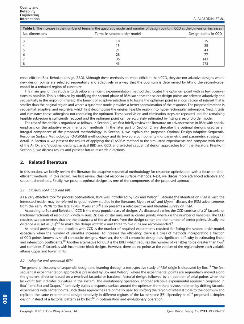
Table I. The increase in the number of terms in the quadratic model and number of design points in CCD as the dimension increases

No. dimensions Terms in second-order model Design points in CCD

3 10 154 15 255 21 436 28 777 36 1438 45 273

A. ALAEDDINI ET AL.

800

more efficient Box–Behnken design (BBD). Although these methods are more efficient than CCD, they are not adaptive designs wherenew design points are selected sequentially and adaptively in a way that the optimum is determined by fitting the second-ordermodel in a reduced region of curvature.

The main goal of this study is to develop an efficient experimentation method that locates the optimum point with as few observa-tions as possible. This is achieved by modifying the second phase of RSM such that the select design points are selected adaptively andsequentially in the region of interest. The benefit of adaptive selection is to locate the optimum point in a local region of interest that issmaller than the original region and where a quadratic model provides a better approximation of the response. The proposed method issequential, adaptive, and recursive, which first decomposes the original feasible region into hyper-rectangular subregions. Next, it testsand eliminates those subregions not containing the optimum. These subdivision and elimination steps are repeated until the remainingfeasible subregion is sufficiently reduced and the optimum point can be accurately estimated by fitting a second-order model.

The rest of the article is organized as follows. In Section 2, we first briefly review the literature on advancements in RSM with specialemphasis on the adaptive experimentation methods. In the later part of Section 2, we describe the optimal designs used as anintegral component of the proposed methodology. In Section 3, we explain the proposed Optimal Design-Adaptive SequentialResponse Surface Methodology (O-ASRSM) methodology and its two core components (nonparametric and parametric strategy) indetail. In Section 4, we present the results of applying the O-ASRSM method to the simulated experiments and compare with thoseof the A-, D-, and V-optimal designs, classical BBD and CCD, and selected sequential design approaches from the literature. Finally, inSection 5, we discuss results and present future research directions.

2. Related literature

In this section, we briefly review the literature for adaptive sequential methodology for response optimization with a focus on data-efficient methods. In this regard, we first review classical response surface methods. Next, we discus more advanced adaptive andsequential methods. Finally, we present optimal designs as one of the components of the proposed approach.

2.1. Classical RSM: CCD and BBD

As a very effective tool for process optimization, RSM was introduced by Box and Wilson.1 Because the literature on RSM is vast, theinterested reader may be referred to good review studies in the literature. Myers et al.6 and Myers7 discuss the RSM advancementsfrom the early 1970s to the late 1990s. Myers et al.8 also presents a retrospective and literature survey on RSM.

According to Box and Behnken,5 CCD is the most popular class of designs. As discussed earlier, the CCD consists of a 2k factorial orfractional factorials of resolution V with nF runs, 2k axial or star runs, and nC center points, where k is the number of variables. The CCDrequires two parameters that are the distance a of the axial runs from the design center and the number of center points. Usually thedistance a is set as (nF)

1/4 to make the design rotatable and three to five runs are recommended.9

As noted previously, one problem with CCD is the number of required experiments required for fitting the second-order model,especially when the number of variables increases. To increase the efficiency, there is a class of methods incorporating a fractionof CCD points, known as small composite designs. However, the small composite design has significant difficulty in estimating linearand interaction coefficients.10 Another alternative for CCD is the BBD, which requires the number of variables to be greater than two5

and combines 2k factorials with incomplete block designs. However, there are no points at the vertices of the region where each variableattains upper and lower limits.

2.2. Adaptive and sequential RSM

The general philosophy of sequential design and learning through a retrospective study of RSM origin is discussed by Box.11 The firstsequential experimentation approach is presented by Box and Wilson,1 where the experimental points are sequentially moved alongthe gradient direction based on a two-level factorial or fractional factorial design, followed by an addition of axial points when thelack-of-fit test indicates curvature in the system. The evolutionary operation, another adaptive experimental approach proposed inBox12 and Box and Draper,13 iteratively builds a response surface around the optimum from the previous iteration by drifting factorialexperiments with center points. Both these approaches are primarily used for shifting the region of interest close to the optimum andreplicate the same experimental design iteratively in different regions of the factor space (FS). Spendley et al.14 proposed a simplexdesign instead of a factorial pattern as by Box12 in optimization and evolutionary operation.


A. ALAEDDINI ET AL.

801

Friedman and Savage15 proposed the one-factor-at-a-time (OFAT) approach, which changes one variable at a time while keepingothers constant at fixed values to find the best response. In this method, once a factor is changed, its value is fixed in the remainder ofthe process, for example, no recurring changes. This process is repeated until all the variables are changed. However, OFAT experimenta-tion is generally discouraged in the literature in comparisonwith factorial design and fractional factorial design (Box et al.,16 Montgomery,9

and Czitrom17). Frey et al.18 introduced the adaptive OFAT (AOFAT) experimentation method, which tends to achieve greater gains thanthose of orthogonal arrays when experimental error is small or the interactions among control factors are large. Frey and Jugulum19 inves-tigate the mechanisms by which AOFAT technique leads to improvement. They investigated conditional main effect, exploitation of aneffect, synergistic interaction, antisynergistic interaction, and overwhelming effect. The AOFAT method is shown to exploit main effectsif interactions are small and exploits two-factor interactions when two-factor interactions are large (Frey and Wang20).

Another adaptive experimentation method is the adaptive response surface method, where in each iteration a portion of thedesign space that corresponds to the response values worse than a given threshold value is discarded.21 When the underlyingfunction is quasi-convex, such elimination reduces the design space gradually to the neighborhood of the global design optimum.However, the number of required design experiments increases exponentially with the number of design variables because adaptiveresponse surface method uses CCD at each iteration and does not inherit any of the previous runs and requires a completely new setof CCD points. Wang22 substitutes CCD with Latin hypercube design to keep some of the points from earlier runs and increase theefficacy. The successive RSM method uses a subspace of the original design as the region of interest to determine an initial approx-imate optimum, which is then improved during the subsequent stages.23 In this method, the new region of interest is centrally builtaround each successive optimum. The improvement in response is attained by moving the center of the region of interest as well aschanging its size through panning and zooming operations, respectively. At each subregion, a D-optimal experimental design is usedto best use the number of available runs together with oversampling to maximize the predictive capability.

To reduce the number of experiments and avoid strong assumptions on the form of the response function, Moore et al.24 designeda response optimization algorithm. Their algorithm tries to determine convex region of interest for performing experiments in eachiteration. To define a neighborhood, they used a geometric procedure that captures the size and shape of the zone of possible opti-mum location(s). Anderson et al.25 developed an efficient nonparametric approach called pairwise bisection for optimizing expensivenoisy function. Their algorithm uses a nonparametric approach to find a geometric relationship among experimented points to findthe optimum effectively. Alaeddini et al.26 proposed an adaptive sequential methodology for responses with two factors, which com-bines the concept of bisection method and classical response surface optimization for reducing the number of required experimentsfor estimating the optimal point. Their methodology uses the information from previous experiments to shrink the FS toward the realoptimum and identify the factor settings of new experiments.

Another adaptive and sequential experimentation research stream that emerges from computer experiments are called surrogatesand extensively used in multidisciplinary design optimization. Sobieszczanski-Sobieski27 proposed concurrent subspace optimizations,where the multidisciplinary systems are linearly decoupled for concurrent optimization. Renaud and Gabriele28 modified this algorithmto build response surface approximations of the objective function and the constraints. Rodríguez et al.29 introduced a general frame-work for surrogate optimization with a trust-region approach. Jones et al.30 proposed an efficient global optimization of expensive blackbox functions. Alexandrov et al.31 developed a trust-region framework for managing the use of approximation models in optimization.Chang et al.32 suggested a stochastic trust-region response-surface method. Gano and Renaud33 introduced a kriging-based scalingfunction to better approximate the high fidelity response on a more global level. Rodríguez et al.34 suggested two sampling strategies,for example, variable and medium fidelity samplings for global optimization. Baumert and Smith35 used pure random search for theglobal optimization of noisy functions and to assess the implications to stochastic global optimization. Jones36 presented a taxonomyof existing approaches for using response surfaces for global optimization. We refer the reader to Sobieszczanski-Sobieski and Haftka,37

Kleijnen,38 Kleijnen et al.,39 Simpson et al.,40 and Chen et al.41 for additional reviews of the studies in this field.

2.3. Optimal design and space-filling sampling

There are multiple optimal designs that differ by the statistical criterion used to select the experiment points. The points are selectedby first determining the region of interest, selecting the number of runs to make, specifying the optimality criterion, and choosing thedesign points from a set of candidate points spaced over the feasible design region. The two earlier studies that greatly contributed tothe development of the idea of optimal designs are Kiefer42,43 and Kiefer and Wolfowitz.44 Optimal designs offer three advantagesover suboptimal experimental designs45: (i) optimal designs reduce the costs of experimentation by allowing statistical models tobe estimated with fewer experimental runs; (ii) optimal designs can accommodate multiple types of factors, such as process, mixture,and discrete factors; and (iii) optimal designs can be optimized with constrained design space, for example, when the mathematicalprocess space contains factor settings that are practically infeasible.

It is known that the least squares estimator minimizes the variance of mean-unbiased estimators. In the estimation theory forstatistical models with one real parameter, the reciprocal of the variance of an (efficient) estimator is called the Fisher informationfor that estimator. Because of this reciprocity, minimizing the variance corresponds to maximizing the information. When the statis-tical model has several parameters, however, the mean of the parameter estimator is a vector, and its variance is a matrix. The inversematrix of the variance matrix is called the information matrix. Because the variance of the estimator of a parameter vector is a matrix,the problem of minimizing the variance is complicated. Using statistical theory, statisticians compress the information matrix usingreal-valued summary statistics; being real-valued functions, these information criteria can be maximized. The traditional optimalitycriteria are invariants of the information matrix; algebraically, the traditional optimality criteria are functions of the eigenvalues ofthe information matrix.46


A. ALAEDDINI ET AL.

802

D-optimal design is the most widely used criterion in optimal designs. A design is said to be D-optimal if |(X0X)� 1| is minimized,which is equivalent to minimizing the volume of the joint confidence region of the vector of regression coefficients or equivalentlymaximizing the differential Shannon information content of the parameter estimates.47 A-optimality seeks to minimize the trace ofthe inverse of the information matrix (Min tr(X0X)� 1). This criterion results in minimizing the average variance of the estimates ofthe regression coefficients. Two other optimal criteria are the G-optimal design that minimizes the maximum scaled predictionvariance over the design region and the V-optimal design that minimizes the average prediction variance over the set of points ofinterest. More recently, Ginsburg and Ben-Gal48 suggest a new design-of-experiment optimality criterion, termed Vs-optimal, forthe robust design of empirically fitted models. Pukelsheim46 provides an excellent source on the optimal design of experiments.

Space-filling designs attempt to spread out the samples as evenly as possible to collect as much information about the entiredesign space as possible. Space-filling methods include orthogonal arrays and various Latin hypercube designs. Latin hypercube isa statistical method for generating a distribution of plausible collections of parameter values from a multidimensional distribution.49

The technique was introduced by McKay et al.50 and further developed by Iman et al.51 More information on the Latin hypercube canbe found in the studies of Tang,52 Park,53 and Ye et al.49 In the context of statistical sampling, a square grid containing sample posi-tions is a Latin square if and only if there is only one sample in each row and each column. A Latin hypercube is the generalization ofthis concept to an arbitrary number of dimensions, whereby each sample is the only one in each axis-aligned hyperplane containingit. Orthogonal sampling adds the requirement that the entire sample space must be sampled evenly.54,55 In other words, orthogonalsampling ensures that the ensemble of random numbers is a very good representative of the real variability. Although orthogonalsampling is generally more efficient, it is more difficult to implement because all random samples must be generated simultaneously.

3. Proposed methodology

O-ASRSM starts with few experiments generated based on an optimal design followed by a nonparametric experiment ranking strat-egy and a parametric quadratic model fitting strategy. The purpose of ranking the experiments is to eliminate those parts of the FSthat are unlikely to contain the real optimal point. The fitting of the quadratic model, which is concurrent to the experiment ranking,finds the approximate location of optimal point. The information from these strategies is combined to determine a reduced FS for thenext run. This procedure continues until the convergence criteria based on the estimated optimal experiment are attained. In the restof this section, we first describe the terminology and state the assumptions in Section 3.1. Next, we provide an overview of themethodology in Section 3.2 and then describe the two core strategies of the O-ASRSM: (i) nonparametric approach in Sections3.3.–3.6 and (ii) parametric approach in Section 3.7. In Section 3.8, we describe how the results of these two strategies are used indesigning the next run of O-ASRSM.

3.1. Terminology and assumptions

For ease of exposition, we first present the definitions and the terminology used in the proposed O-ASRSM method in the next section.Figure 1 illustrates some of the notations for a two-dimensional FS with five initial experiments:

r

Figure 1.

Copyrigh

: index of runs, for example, r= 1, 2, . . . R, where R is the total number of runs.
FSr : factor space at run r and expressed as Cartesian product of factor ranges in run r. n : number of factors in the FS. f si : initial range of factor i. D : design of the incumbent run. d : minimum number of required points to estimate quadratic regression parameters (d= (n2 + 3n+ 4)/2). e : index of experiments, for example, e = 1,2,. . .,E, where E is the total number of experiments. B : experiment with the best response level in a given run.
B

N3

N5

N6

WN7

\

after the initialrun (based on ranking)

Legend

Additional after two more experiments (based on ranking)

B

N2

N4

WN5

N3N4

N2

(a) (b)

Additional experiments

Estimated Optimal (EO) point (based on parametric strategic)

Initial run’s experiments

An illustration of terminology on a two-dimensional FS: (a) eliminated subregions (NORs) after first five experiments; (b) eliminated subregions (NORs) afteradditional two experiments

t © 2012 John Wiley & Sons, Ltd. Qual. Reliab. Engng. Int. 2013, 29 799–817

A. ALAEDDINI ET AL.

Nk

Figure 2.

Copyrigh

: experiment with the kth best response level (2⩽ k⩽ e� 1) in a given run.
W : experiment with the worst response level in a given run. ORr : optimal region after the rth run. NOR : nonoptimal region, for example, regions declared as not containing the optimum experiment. RO : real optimum experiment of the response function. EOr : estimated optimum experiment at the end of the rth run. sb : index of subregions for a given factor, for example, sb=1, 2 . . ., kn, where kn is the total number of subregions E* : total number of augmenting experiments. Ssb : size of subregion sb.
The proposed O-ASRSM method, as in most RSM approaches, relies on the simplifying assumption of quadratic relation betweenthe single response and the input factors. The reason is that RSM models are usually used in a sufficiently small region around theoptimum experiment. As a result, it is commonly assumed in RSM applications that the underlying model can be approximated viaa quadratic function in the small region of interest containing the optimum experiment. Such assumption also holds for this study;however, as shown in the numerical example section, the proposed method is robust with regard to this assumption.

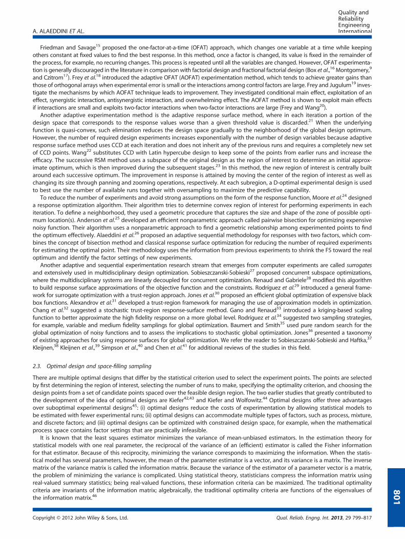
3.2. General scheme of the proposed methodology

We illustrate the general scheme of the proposed methodology in Figure 2. The procedure is initialized with a region of interest, forexample, an FS assumed to contain the optimum. The goal is to arrive at the vicinity of RO in finite number of experiments. The initialrun is setup with an optimal design (D) using minimum number of experiments possible and then augmented with E* additionalexperiments. Once the experimentation is completed, the approach follows two concurrent (parallel) strategies: (i) nonparametricranking strategy and (ii) parametric model fitting strategy.

The main objective of the nonparametric strategy is to identify those parts of the FS that have a small probability of containing thereal optimal point. For this purpose, the nonparametric strategy partitions the FS into a set of subregions (sb). Next, it uses the observedrank of experiments to construct a system of quadratic inequalities for each sb to check their possibility of containing the real optimalpoint (RO). In Section 3.4, we prove that the feasible solution of the system of equation for each sb is equivalent to the sb containing theRO and vice versa. The subregions that do not contain RO are indicated as NORs and the rest are labeled as ORs. Therefore, by applyingthe nonparametric strategy, the NORs are excluded from further experimentation in the subsequent iterations.

Initialize:• Label the first run (r=1) • Determine the design D based on an optimal

design with smallest number of experiments

Experimentation:• Take the experiment/s one at a time based on

design D

FS partitioning:• Partition the factor space into a set of sub-

regions ( ) with similar structure to

Model fitting:• Fit the quadratic model using the E

experiments in the current run

Converged?

RO Estimation:• Determine the optimal point • Stop

Yes

Parametric Approach (Model Fitting Strategy)

Design Augmentation:• Design augmenting experiments on the new

factor space and set r=r+1

No

Experiments Ranking:• Rank the experiments in the current run as B,

N2,…, Nk, ,W

FS Reduction:• Design a system of quadratic inequalities • solve it for each sub-region to check if it can

be labeled as and removed

E d

NoNon-parametric Approach

(Ranking Strategy)Yes

Indentifying EO:• Solve the fitted model to estimate the

optimal point (EOr)

The general scheme of O-ASRSM

t © 2012 John Wiley & Sons, Ltd. Qual. Reliab. Engng. Int. 2013, 29 799–817

803

A. ALAEDDINI ET AL.

804

The main objectives of the parametric strategy are providing a point estimate (EO) of the real optima and checking the conver-gence of the algorithm. The parametric strategy fits a quadratic model using all the experiments and determines the EO. Next, itchecks the convergence of the algorithm based on the incremental change in the (|Δ(EO)|⩽ dEO).

On the basis of the result of parametric strategy, if the stopping a criterion is not met (|Δ(EO)|⩽ dEO), the O-ASRSM algorithmproceeds to another run of experimentation and analysis by determining a reduced FS (FSr+1) for of the next run (r+ 1) using onlythe ORs indentified by the nonparametric strategy. This procedure continues until the convergence criteria, incremental change inthe EO being less than the tolerance specified, is attained.

3.3. Design structure of experimental runs

The designD structure of the FS in the proposed approach is adapted from the D-optimal design usingminimum number of experiments.This design may be further augmented with E* additional experiments in the identified ORs of the FS as discussed in Section 3.7.

The FS of each run r (FSr) can be expressed as a mapping (’r) of the FS of the preceding iteration (FSr�1). In its most generalform, the proposed methodology generates a nested series of FSs, for example, FSr=’r(’r� 1(. . .’0(FS1))). The output of map-ping ’r? depends on the current FS, the experimentation design (D), the experiment ranking outcome, and the result of theparametric strategy described in the next section. The ranking and the parametric strategies are described in Sections 3.4 and3.8, respectively.

In the traditional CCD and BBD approaches, the corner points are taken at � 1 unit distance away from the center point (0,0). Incontrast, the proposed methodology, whenever it is possible, starts with a broader initial region around the center point, forexample, � 2n/4 unit distance from the center. The preceding relation is based on the calculation of axial points in rotatableCCD with single replicate at all designated points.9 While initializing with a larger space may appear to be disadvantageous forO-ASRSM, our experimental results demonstrate that the reduction in the FS with the equal number of experiments well compen-sates for this difference. As an additional benefit, this modification may decrease the effect of random error on the initial results. Toillustrate this, let us consider the diagonal cross section of these two designs in one dimension and assume that the noise is iden-tically distributed on this cross section (Figure 3b). Then, it can be shown that the impact of the noise in predicting the optimalexperiment point is less with the O-ASRSM’s expanded FS. Figure 3 compares the initial FS of the traditional CCD and the proposedapproach for a two-dimensional FS.

3.4. Nonparametric approach: ranking strategy

At each stage of the O-ASRSM, we rank the experiments according to their response levels, for example, from best (B) to worst (W),and the rankings in between are labeled as N2 . . .,N(k� 1). On the basis of this ranking, we remove the nonpromising subregions(NORs) from further consideration as they are determined to not to contain the RO. The remaining subregions identify an impliedoptimal region that contains the EOr. This region, which is contained in FS (can be a convex or nonconvex set), determines the FSof the next run. In what follows, we first present the theorem used for the identification of the NORs inside an FS. Next, we describehow to reduce the FS by removing the nonoptimal subregions. Finally, we describe how to choose additional experiments in the finalstep of the nonparametric ranking strategy.

Theorem 1:Let FS be a hyper-rectangular region of n dimensions with E experiments placed inside the region based on an optimal design. Also,assume E is greater than or equal to the minimum number of the required points to estimate quadratic regression parameters E⩾ d. Ifthe underlying function is quadratic and convex, and the true ranking of experiments is available, then using the ranking at least onesubregion of nonzero size {Ssb|Ssb> 0, sb2 FS} can be identified inside FS which is guaranteed not to contain the RO.

(b)(a)

+1 +1.4142-1.4142 -1 0

Proposed Approach

initial range

CCD

initial range

d=

d=

Figure 3. (a) Initial FS and design structure and (b) diagonal cross section of the traditional CCD and proposed O-ASRSM approach


A. ALAEDDINI ET AL.

ProofDivide the hyper-rectangular FS into a set of kn (k> 1) subregions with equal sizes (dx1, . . ., dxn) in all dimensions. Because the underlyingfunction is assumed to be convex and unimodal, there is only one subregion containing the RO, and kn� 1 subregions not containingRO. It should be noted that because we use optimal design for D, the experiments are expected to not form a cluster in any subregion ofthe FS. If not, we can resize those subregions such that each experiment is contained in only one subregion.

Let us assume the optimal point, denoted by O , resides in the subregion containing W, the worst experiments. Then, for each

experiment 1< e⩽ E, we express the response model in a canonical form as Ze ¼Pn

i;j¼1Ai;j Xei � XO

i

� �Xej � XO

j

� �þPn

i¼1Bi Xei � XO

i

� �þ Re , where Ai, j2 R and Re are constants. Because the canonical form must be consistent with empirical ranks of

the experiments (B<N2<⋯<Nk<W), we can sort the canonical forms of the experiments in an ascending order

ZeB < ZeN2 < ⋯ < ZeW

� �. Next, on the basis of the sorted experiments, we formulate a system of inequalities with E(E� 1)/2 pairwise

comparisons as follows:

ZeB � ZeN2 ¼Xni;j¼1

Ai;j XeBi � XO

i

� �XeBj � XOj

� �þXni¼1

Bi XeBi � XO

i

� �" #�

Xni;j¼1

Ai;j XeN2i � XO

i

� �XeN2j � XO

j

� �þXni¼1

Bi XeN2i � XO

i

� �" #< 0:

ZeN2 � ZeN3 ¼Xni;j¼1

Ai;j XeN2i � XO

i

� �XeN2j � XO

j

� �þXni¼1

Bi XeN2i � XO

i

� �" #�

Xni;j¼1

Ai;j XeN3i � XO

i

� �XeN3j � XO

j

� �þXni¼1

Bi XeN3i � XO

i

� �" #< 0:

⋮ ⋮ ⋮

ZeNk � ZeW ¼Xni;j¼1

Ai;j XeNki � XO

i

� �XeNkj � XOj

� �þXni¼1

Bi XeNki � XO

i

� �" #�

Xni;j¼1

Ai;j XeWi � XO

i

� �XeWj � XO

j

� �þXni¼1

Bi XeWi � XO

i

� �" #< 0:

8>>>>>>>>>>>>><>>>>>>>>>>>>>:

(2)

where Ai, j, Bi, and XOj are the unknowns and XO

j is bounded by the boundaries of the subregion hypothesized to contain O . Ifpreviously mentioned system of quadratic inequalities does not have a feasible solution, the candidate subregion cannot containRO and vice versa.

Each of the inequalities in Equation (2) compares the canonical quadratic distance between a pair of experiments, for example, W

and B, to O. Given that O is contained in the same sb withW, as the size of sb (Ssb) decreases, the canonical quadratic distance ofW willbe less than other experiments (with better ranks), making the system of inequalities (Equation (2)) infeasible. Because this contradictsthe existence of RO in one of the subregions, the proof is complete.

The following example illustrates the previously mentioned proof using a simple two-dimensional FS.

3.4.1. Example: analysis for existence and size of an NOR subregion in a sample with two-dimensional FS. Figure 4 illustrates two-dimensional FS of unit length with seven experiments from a D-optimal design. We consider uniform grid for subregions, for example,dxi= a for i=1, 2. For the candidate subregion where W experiment resides on the northeast corner, the system of quadratic equationscan be written as

B

N2

Lx2=1

N3

N4

W

dx1=

dx2=N6

N7

Hypothetical

location for

Lx1=1

Figure 4. Two-dimensional FS with seven experiments based on D-optimal design


805

A. ALAEDDINI ET AL.

806

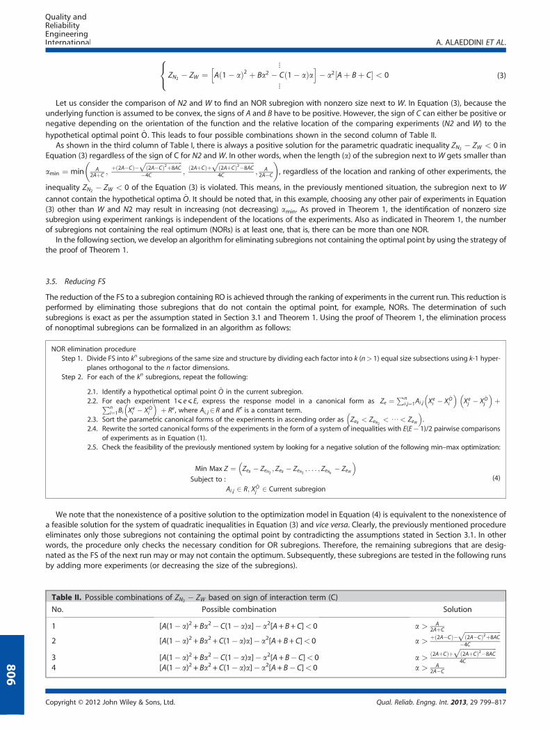
⋮ZN2 � ZW ¼ A 1� að Þ2 þ Ba2 � C 1� að Þa

h i� a2 Aþ Bþ C½ � < 0

⋮

8<: (3)

Let us consider the comparison of N2 and W to find an NOR subregion with nonzero size next to W. In Equation (3), because theunderlying function is assumed to be convex, the signs of A and B have to be positive. However, the sign of C can either be positive ornegative depending on the orientation of the function and the relative location of the comparing experiments (N2 and W) to the

hypothetical optimal point O. This leads to four possible combinations shown in the second column of Table II.As shown in the third column of Table I, there is always a positive solution for the parametric quadratic inequality ZN2 � ZW < 0 in

Equation (3) regardless of the sign of C for N2 andW. In other words, when the length (a) of the subregion next toW gets smaller than

amin ¼ min A2AþC ;

þ 2A�Cð Þ�ffiffiffiffiffiffiffiffiffiffiffiffiffiffiffiffiffiffiffiffiffi2A�Cð Þ2þ8AC

p�4C ;

2AþCð Þþffiffiffiffiffiffiffiffiffiffiffiffiffiffiffiffiffiffiffiffiffi2AþCð Þ2�8AC

p4C ; A

2A�C

� �, regardless of the location and ranking of other experiments, the

inequality ZN2 � ZW < 0 of the Equation (3) is violated. This means, in the previously mentioned situation, the subregion next to W

cannot contain the hypothetical optima O. It should be noted that, in this example, choosing any other pair of experiments in Equation(3) other than W and N2 may result in increasing (not decreasing) amin. As proved in Theorem 1, the identification of nonzero sizesubregion using experiment rankings is independent of the locations of the experiments. Also as indicated in Theorem 1, the numberof subregions not containing the real optimum (NORs) is at least one, that is, there can be more than one NOR.

In the following section, we develop an algorithm for eliminating subregions not containing the optimal point by using the strategy ofthe proof of Theorem 1.

3.5. Reducing FS

The reduction of the FS to a subregion containing RO is achieved through the ranking of experiments in the current run. This reduction isperformed by eliminating those subregions that do not contain the optimal point, for example, NORs. The determination of suchsubregions is exact as per the assumption stated in Section 3.1 and Theorem 1. Using the proof of Theorem 1, the elimination processof nonoptimal subregions can be formalized in an algorithm as follows:

NOR elimination procedure

Ta

No

1

2

34

Copy

Step 1. Divide FS into kn subregions of the same size and structure by dividing each factor into k (n> 1) equal size subsections using k-1 hyper-planes orthogonal to the n factor dimensions.

Step 2. For each of the kn subregions, repeat the following:

ble II. P

.

right ©

2.1. Identify a hypothetical optimal point O in the current subregion.2.2. For each experiment 1⩽ e⩽ E, express the response model in a canonical form as Ze ¼

Pni;j¼1Ai;j Xe

i � XOi

� �Xej � XO

j

� �þPn

i¼1Bi Xei � XO

i

� �þ Re, where Ai, j2 R and Re is a constant term.

2.3. Sort the parametric canonical forms of the experiments in ascending order as ZeB < ZeN2 < ⋯ < ZeW

� �.

2.4. Rewrite the sorted canonical forms of the experiments in the form of a system of inequalities with E(E� 1)/2 pairwise comparisonsof experiments as in Equation (1).

2.5. Check the feasibility of the previously mentioned system by looking for a negative solution of the following min–max optimization:

Min Max Z ¼ ZeB � ZeN2 ; ZeB � ZeN2 ; . . . ; ZeNk � ZeW

� �Subject to :

Ai;j 2 R; XOj 2 Current subregion

(4)

We note that the nonexistence of a positive solution to the optimization model in Equation (4) is equivalent to the nonexistence ofa feasible solution for the system of quadratic inequalities in Equation (3) and vice versa. Clearly, the previously mentioned procedureeliminates only those subregions not containing the optimal point by contradicting the assumptions stated in Section 3.1. In otherwords, the procedure only checks the necessary condition for OR subregions. Therefore, the remaining subregions that are desig-nated as the FS of the next run may or may not contain the optimum. Subsequently, these subregions are tested in the following runsby adding more experiments (or decreasing the size of the subregions).

ossible combinations of ZN2 � ZW based on sign of interaction term (C)

Possible combination Solution

[A(1� a)2 + Ba2� C(1� a)a]� a2[A+ B+C]< 0 a > A2AþC

[A(1� a)2 + Ba2 + C(1� a)a]� a2[A+ B+C]< 0 a >þ 2A�Cð Þ�

ffiffiffiffiffiffiffiffiffiffiffiffiffiffiffiffiffiffiffiffiffi2A�Cð Þ2þ8AC

p�4C

[A(1� a)2 + Ba2� C(1� a)a]� a2[A+ B�C]< 0 a >2AþCð Þþ

ffiffiffiffiffiffiffiffiffiffiffiffiffiffiffiffiffiffiffiffiffi2AþCð Þ2�8AC

p4C

[A(1� a)2 + Ba2 + C(1� a)a]� a2[A+ B�C]< 0 a > A2A�C

2012 John Wiley & Sons, Ltd. Qual. Reliab. Engng. Int. 2013, 29 799–817

A. ALAEDDINI ET AL.

3.6. Computational complexity and accuracy of NOR elimination procedure

The computational complexity and accuracy of NOR elimination procedure depends on three variables, E, n, and k:

(1) E, the number of experiments, affects the number of quadratic inequalities (NIQ) in the system of quadratic inequalities by a

polynomial order NIQ ¼ E E�1ð Þ2

� �.

(2) n, the number of dimensions, affects both the number of variables in quadratic inequalities (V) by a polynomial order

V ¼ 3n1

� �þ n

2

� �� and the number of procedure iterations (PI) by an exponential order (PI = kn).

(3) k, the number of divisions in each FS, affects the number of the procedure iterations (PI) by an exponential order (PI = kn).

As a result, the complexity of the elimination procedure grows exponentially with increasing n and k. In other words, O-ASRSMtrades off between the total number of experiments and the computational complexity of the algorithm. In most practical cases,the computational effort necessary is negligible, either due to the existence of powerful computational resources (e.g. parallelcomputing facilities) or due to experiments being too costly vis-à-vis the computational effort. In other cases, the choice of k can savethe computational effort considerably while keeping the accuracy of the algorithm at an acceptable level.

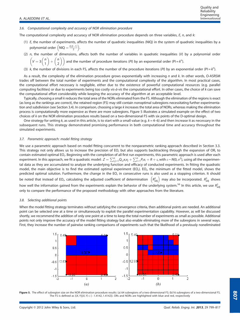
Typically, choosing a small k reduces the total area of the NORs eliminated from the FS. Although the elimination of the regions is exact(as long as the rankings are correct), the retained region (FS) may still contain nonoptimal subregions necessitating further experimenta-tion and subdivision (see Section 3.4). In comparison, choosing a large k increases the total area of NORs, whereas making the eliminationprocess is computationally more expensive as there are more subregions. Figure 5 illustrates a simulated example on the effect of twochoices of k on the NOR elimination procedure results based on a two-dimensional FS with six points of the D-optimal design.

One strategy for setting k, as used in this article, is to start with a small value (e.g. k = 4–6) and then increase it as necessary in thesubsequent runs. This strategy demonstrated promising performance in both computational time and accuracy throughout thesimulated experiments.

3.7. Parametric approach: model fitting strategy

We use a parametric approach based on model fitting concurrent to the nonparametric ranking approach described in Section 3.3.This strategy not only allows us to increase the precision of EOr but also supports backtracking through the expansion of ORr tocontain estimated optimal EOr. Beginning with the completion of all first run experiments, this parametric approach is used after eachexperiment. In this approach, we fit a quadratic model: Z ¼ Pn

i;j¼1Qi;jxixj þPn

i¼1Pixi þ Rþ e, with e~N(0,s2), using all the experimen-

tal data as they are accumulated to analyze the underlying function and efficacy of conducted experiments. In fitting the quadraticmodel, the main objective is to find the estimated optimal experiment (EOr). EOr, the minimum of the fitted model, shows thepredicted optimal solution. Furthermore, the change in the EOr in consecutive runs is also used as a stopping criterion. It should

be noted that instead of EOr, calculating the adjusted coefficient of determination R2adj

� �may also be incorporated. R2adj shows

how well the information gained from the experiments explain the behavior of the underlying system.56 In this article, we use R2adjonly to compare the performance of the proposed methodology with other approaches from the literature.

3.8. Selecting additional points

When the model fitting strategy terminates without satisfying the convergence criteria, then additional points are needed. An additionalpoint can be selected one at a time or simultaneously to exploit the parallel experimentation capability. However, as will be discussedshortly, we recommend the addition of only one point at a time to keep the total number of experiments as small as possible. Additionalpoints not only improve the accuracy of the model fitting strategy but also enable eliminating more of the subregions in several ways.First, they increase the number of pairwise ranking comparisons of experiments such that the likelihood of a previously noneliminated

(a) (b)

Figure 5. The effect of subregion size on the NOR elimination procedure results: (a) 64 subregions of a two-dimensional FS; (b)16 subregions of a two-dimensional FS.The FS is defined as {(X, Y)|(X, Y)2 [�1.4142, 1.4142]}. ORs and NORs are highlighted with blue and red, respectively


807

A. ALAEDDINI ET AL.

808

subregion becoming a NOR is increased. Second, with these additional points, the new ranking of the experiments leads to a bettercoverage of FS. Finally, additional points result in more reliable ranking of the experiments when the underlying function is noisy. Thenecessary condition for the above claims is that the additional points do not change the characterization of previously labeled NORsubregion, which can be provenwhen the underlying function is convex quadratic and deterministic. The following proposition guaranteesthe consistent characterization of the NOR through adding additional points:

Proposition 1:If the underlying function is convex quadratic and without noise, then the addition of experiment(s) to the rth run FS does not reducethe size of the NORs identified in the ((r� 1)th run.

ProofLet E denote the number of experiments at the (r� 1)th run where the FS (FSr� 1) has been divided into kn subregions. The necessarycondition for optimality of each subregion is the feasible solution of the system of Equation (1), consisting of E(E� 1)/2 inequalities atthe (r� 1)th run. Adding F new experiments to the design in the next run (r) will add (E+ F)(E+ F� 1)/2� E(E� 1)/2 inequalities toEquation (1) for each subregion while preserving the previous inequalities. This addition of constraints only reduces the feasible spaceof Equation (1), which clearly does not cause NORs to become ORs. Therefore, the addition of point(s) to the FS in a run will not reducethe size of the previous run’s NORs. □

Corollary 1:If the underlying function is convex quadratic and without noise, then NORs and ORs across NOR elimination procedures are nonde-creasing and nonincreasing sets, respectively.

ProofOn the basis of Proposition 1, additional experiments do not decrease the NORs. Therefore, moving from one run to the next, bypotentially including additional runs, NORs will not decrease or equivalently ORs are nonincreasing.

Corollary 1 shows that the FS area can be reduced toward the optimal point by adding more experiments. However, because oneof the goals of O-ASRSM is to reduce the total number of experiments, the number of additional points (E*) should be kept as small aspossible, preferably by adding one at a time. For this purpose, each of the additional points can be selected by implementing an aug-mented optimal design with E* experiments (in this study we use E* = 1) on the remaining parts of FSr� 1, after eliminating the NORs(ORr� 1 = FSr). Augmentation of the optimal design D with respect to ORr� 1 can be performed by adding a total ofm� 2n constraints,where m is the number of NORs and n is the number of factors, to the objective function of the optimal design. Each set of 2n con-straints is for turning one of NORs to unfeasible parts of FSr, where each constraint can be written as

Yn

i¼1

max Xi � XiLð Þ; 0½ �Xi � XiLð Þ �max XiU � Xið Þ; 0½ �

XiU � Xið Þ ¼ 0 (5)

In Equation (5), XiL ; XiUð Þ are the lower and upper bounds of the selected NOR subregion. The denominators in Equation (5) are usedfor scaling purposes such that the left-hand side of the equation becomes either 0 or 1. Note that this approach could also be used totackle simple bound constraints within the O-ASRSM method, thereby making it applicable to a broader range of engineering designproblems, for example, constrained problems with simple bound constraints.

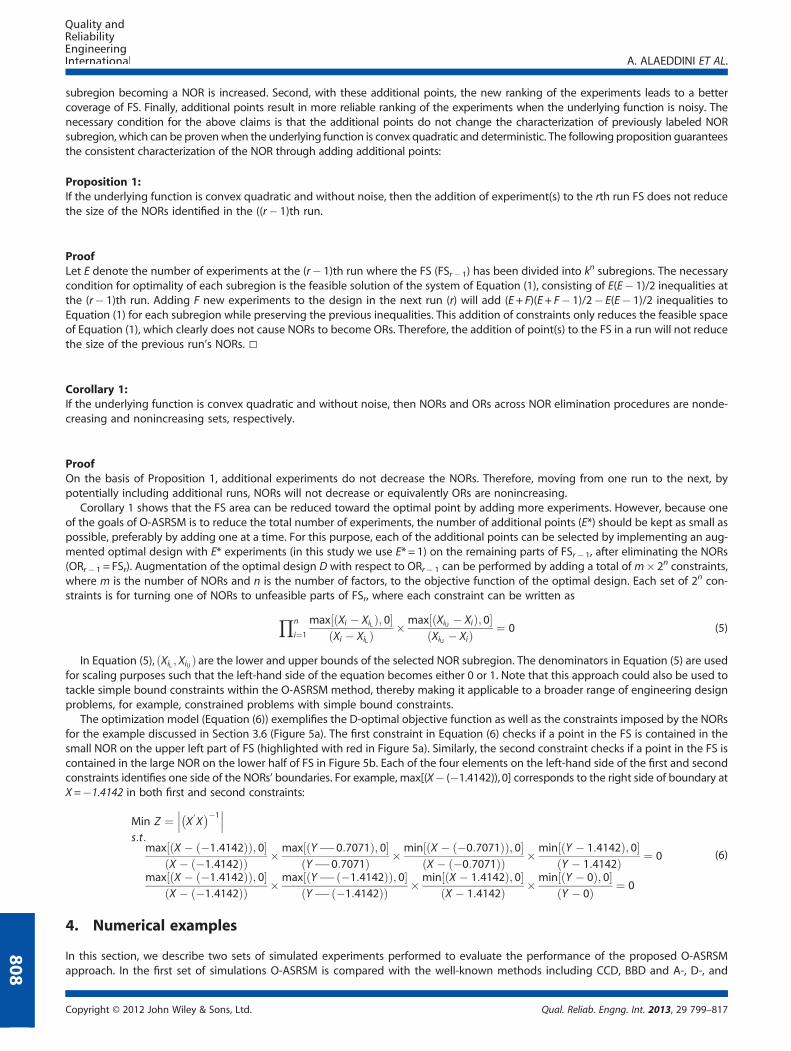
The optimization model (Equation (6)) exemplifies the D-optimal objective function as well as the constraints imposed by the NORsfor the example discussed in Section 3.6 (Figure 5a). The first constraint in Equation (6) checks if a point in the FS is contained in thesmall NOR on the upper left part of FS (highlighted with red in Figure 5a). Similarly, the second constraint checks if a point in the FS iscontained in the large NOR on the lower half of FS in Figure 5b. Each of the four elements on the left-hand side of the first and secondconstraints identifies one side of the NORs’ boundaries. For example, max[(X� (�1.4142)), 0] corresponds to the right side of boundary atX=�1.4142 in both first and second constraints:

Min Z ¼ X0X

� ��1

s:t:max X � �1:4142ð Þð Þ; 0½ �

X � �1:4142ð Þð Þ �max Y�0:7071ð Þ; 0½ �Y�0:7071ð Þ �min X � �0:7071ð Þð Þ; 0½ �

X � �0:7071ð Þð Þ �min Y � 1:4142ð Þ; 0½ �Y � 1:4142ð Þ ¼ 0

max X � �1:4142ð Þð Þ; 0½ �X � �1:4142ð Þð Þ �max Y� �1:4142ð Þð Þ; 0½ �

Y� �1:4142ð Þð Þ �min X � 1:4142ð Þ; 0½ �X � 1:4142ð Þ �min Y � 0ð Þ; 0½ �

Y � 0ð Þ ¼ 0

(6)

4. Numerical examples

In this section, we describe two sets of simulated experiments performed to evaluate the performance of the proposed O-ASRSMapproach. In the first set of simulations O-ASRSM is compared with the well-known methods including CCD, BBD and A-, D-, and


A. ALAEDDINI ET AL.

V-optimal designs using different quadratic response models with varying variance of errors. The second set of simulations study theperformance of the proposed approach along with classical models, optimal designs and two global optimization methods (Standleret al.23 Wang22) on several nonlinear response models with varying levels of noise.

4.1. Quadratic response models

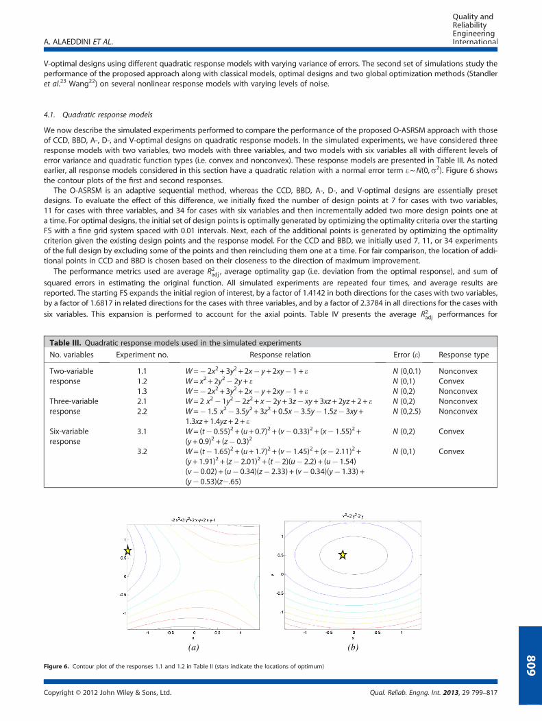
We now describe the simulated experiments performed to compare the performance of the proposed O-ASRSM approach with thoseof CCD, BBD, A-, D-, and V-optimal designs on quadratic response models. In the simulated experiments, we have considered threeresponse models with two variables, two models with three variables, and two models with six variables all with different levels oferror variance and quadratic function types (i.e. convex and nonconvex). These response models are presented in Table III. As notedearlier, all response models considered in this section have a quadratic relation with a normal error term e~N(0,s2). Figure 6 showsthe contour plots of the first and second responses.

The O-ASRSM is an adaptive sequential method, whereas the CCD, BBD, A-, D-, and V-optimal designs are essentially presetdesigns. To evaluate the effect of this difference, we initially fixed the number of design points at 7 for cases with two variables,11 for cases with three variables, and 34 for cases with six variables and then incrementally added two more design points one ata time. For optimal designs, the initial set of design points is optimally generated by optimizing the optimality criteria over the startingFS with a fine grid system spaced with 0.01 intervals. Next, each of the additional points is generated by optimizing the optimalitycriterion given the existing design points and the response model. For the CCD and BBD, we initially used 7, 11, or 34 experimentsof the full design by excluding some of the points and then reincluding them one at a time. For fair comparison, the location of addi-tional points in CCD and BBD is chosen based on their closeness to the direction of maximum improvement.

The performance metrics used are average R2adj , average optimality gap (i.e. deviation from the optimal response), and sum of

squared errors in estimating the original function. All simulated experiments are repeated four times, and average results arereported. The starting FS expands the initial region of interest, by a factor of 1.4142 in both directions for the cases with two variables,by a factor of 1.6817 in related directions for the cases with three variables, and by a factor of 2.3784 in all directions for the cases with

six variables. This expansion is performed to account for the axial points. Table IV presents the average R2adj performances for

Table III. Quadratic response models used in the simulated experiments

No. variables Experiment no. Response relation Error (e) Response type

Two-variableresponse

1.1 W=� 2x2 + 3y2 + 2x� y+2xy� 1 + e N (0,0.1) Nonconvex1.2 W= x2 + 2y2� 2y+ e N (0,1) Convex1.3 W=� 2x2 + 3y2 + 2x� y+2xy� 1 + e N (0,2) Nonconvex

Three-variableresponse

2.1 W= 2 x2� 1y2� 2z2 + x� 2y+ 3z� xy+ 3xz+ 2yz+ 2+ e N (0,2) Nonconvex2.2 W=� 1.5 x2� 3.5y2 + 3z2 + 0.5x� 3.5y� 1.5z� 3xy+

1.3xz+ 1.4yz+ 2+ eN (0,2.5) Nonconvex

Six-variableresponse

3.1 W= (t� 0.55)2 + (u+0.7)2 + (v� 0.33)2 + (x� 1.55)2 +(y+ 0.9)2 + (z� 0.3)2

N (0,2) Convex

3.2 W= (t� 1.65)2 + (u+1.7)2 + (v� 1.45)2 + (x� 2.11)2 +(y+ 1.91)2 + (z� 2.01)2 + (t� 2)(u� 2.2) + (u� 1.54)(v� 0.02) + (u� 0.34)(z� 2.33) + (v� 0.34)(y� 1.33) +(y� 0.53)(z�.65)

N (0,1) Convex

(a) (b)

Figure 6. Contour plot of the responses 1.1 and 1.2 in Table II (stars indicate the locations of optimum)


809

Table

IV.R2 ad

jfortrials7,8,an

d9ofthequad

raticresponseswithtw

ovariab

les;trials11

,12,an

d13

ofthequad

raticresponseswiththreevariab

les;an

dtrials34

,35an

d36

ofthe

quad

raticresponseswithsixvariab

les

Adjusted

R2

Experim

entno.

No.o

bservation

CCD

BBD

O-ASR

SMD-optimal

V-optimal

A-optimal

1.1

799

.96%

N/A

99.99%

99.96%

99.92%

99.94%

899

.96%

N/A

99.99%

99.98%

99.95%

99.95%

999

.95%

N/A

99.99%

99.97%

99.94%

99.92%

1.2

792

.69%

N/A

98.74%

95.01%

94.85%

90.69%

892

.48%

N/A

98.42%

89.20%

95.86%

86.86%

992

.00%

N/A

97.15%

90.42%

95.42%

86.58%

1.3

769

.77%

N/A

92.95%

92.96%

72.11%

97.71%

870

.60%

N/A

94.59%

91.06%

74.92%

79.86%

988

.48%

N/A

95.55%

89.02%

80.89%

82.00%

Ave.

787

.47%

N/A

97.23%

95.98%

88.96%

96.11%

887

.68%

N/A

97.67%

93.41%

90.24%

88.89%

993

.48%

N/A

97.56%

93.14%

92.08%

89.50%

2.1

1187

.30%

76.11%

93.13%

98.18%

92.66%

98.42%

1288

.10%

81.32%

96.29%

98.61%

95.60%

96.60%

1391

.09%

79.87%

98.32%

97.66%

95.67%

97.79%

2.2

1189

.02%

53.12%

98.39%

89.25%

84.88%

90.50%

1287

.06%

56.04%

97.37%

92.93%

86.88%

91.76%

1386

.50%

49.48%

95.36%

91.74%

88.27%

90.12%

Average

1188

.16%

64.62%

95.76%

93.72%

88.77%

94.46%

1287

.58%

68.68%

96.83%

95.77%

91.24%

94.18%

1388

.80%

64.68%

96.84%

94.70%

91.97%

93.96%

3.1

3480

.21%

70.00%

98.63%

90.20%

96.49%

90.20%

3579

.61%

70.10%

98.94%

91.84%

96.76%

91.84%

3679

.82%

64.18%

99.05%

92.73%

97.26%

92.73%

3.2

3499

.56%

98.27%

99.92%

97.80%

99.93%

99.82%

3599

.55%

98.27%

99.94%

99.81%

99.94%

99.85%

3699

.55%

98.27%

99.95%

99.82%

99.94%

99.81%

3489

.89%

84.14%

99.28%

94.00%

98.21%

95.01%

Average

3589

.58%

84.19%

99.44%

95.83%

98.35%

95.85%

3689

.69%

81.23%

99.50%

96.28%

98.60%

96.27%

A. ALAEDDINI ET AL.


810

A. ALAEDDINI ET AL.

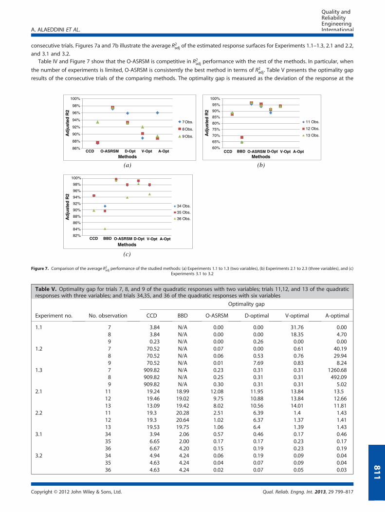
consecutive trials. Figures 7a and 7b illustrate the average R2adj of the estimated response surfaces for Experiments 1.1–1.3, 2.1 and 2.2,

and 3.1 and 3.2.Table IV and Figure 7 show that the O-ASRSM is competitive in R2adj performance with the rest of the methods. In particular, when

the number of experiments is limited, O-ASRSM is consistently the best method in terms of R2adj. Table V presents the optimality gap

results of the consecutive trials of the comparing methods. The optimality gap is measured as the deviation of the response at the

86%

88%

90%

92%

94%

96%

98%

100%

Ad

just

ed R

2

Methods

7 Obs.

8 Obs.

9 Obs.

60%

65%

70%

75%

80%

85%

90%

95%

100%

Ad

just

ed R

2

Methods

11 Obs.

12 Obs.

13 Obs.

(a) (b)

82%

84%

86%

88%

90%

92%

94%

96%

98%

100%

Ad

just

ed R

2

Methods

34 Obs.

35 Obs.

36 Obs.

(c)

CCD

CCD

D-OptO-ASRSM V-Opt A-Opt CCD D-OptO-ASRSM

O-ASRSM

BBD

BBD

V-Opt A-Opt

D-Opt V-Opt A-Opt

Figure 7. Comparison of the average R2adj performance of the studied methods: (a) Experiments 1.1 to 1.3 (two variables), (b) Experiments 2.1 to 2.3 (three variables), and (c)Experiments 3.1 to 3.2

Table V. Optimality gap for trials 7, 8, and 9 of the quadratic responses with two variables; trials 11,12, and 13 of the quadraticresponses with three variables; and trials 34,35, and 36 of the quadratic responses with six variables

Optimality gap

Experiment no. No. observation CCD BBD O-ASRSM D-optimal V-optimal A-optimal

1.1 7 3.84 N/A 0.00 0.00 31.76 0.008 3.84 N/A 0.00 0.00 18.35 4.709 0.23 N/A 0.00 0.26 0.00 0.00

1.2 7 70.52 N/A 0.07 0.00 0.61 40.198 70.52 N/A 0.06 0.53 0.76 29.949 70.52 N/A 0.01 7.69 0.83 8.24

1.3 7 909.82 N/A 0.23 0.31 0.31 1260.688 909.82 N/A 0.25 0.31 0.31 492.099 909.82 N/A 0.30 0.31 0.31 5.02

2.1 11 19.24 18.99 12.08 11.95 13.84 13.512 19.46 19.02 9.75 10.88 13.84 12.6613 13.09 19.42 8.02 10.56 14.01 11.81

2.2 11 19.3 20.28 2.51 6.39 1.4 1.4312 19.3 20.64 1.02 6.37 1.37 1.4113 19.53 19.75 1.06 6.4 1.39 1.43

3.1 34 3.94 2.06 0.57 0.46 0.17 0.4635 6.65 2.00 0.17 0.17 0.23 0.1736 6.67 4.20 0.15 0.19 0.23 0.19

3.2 34 4.94 4.24 0.06 0.19 0.09 0.0435 4.63 4.24 0.04 0.07 0.09 0.0436 4.63 4.24 0.02 0.07 0.05 0.03


811

A. ALAEDDINI ET AL.

812

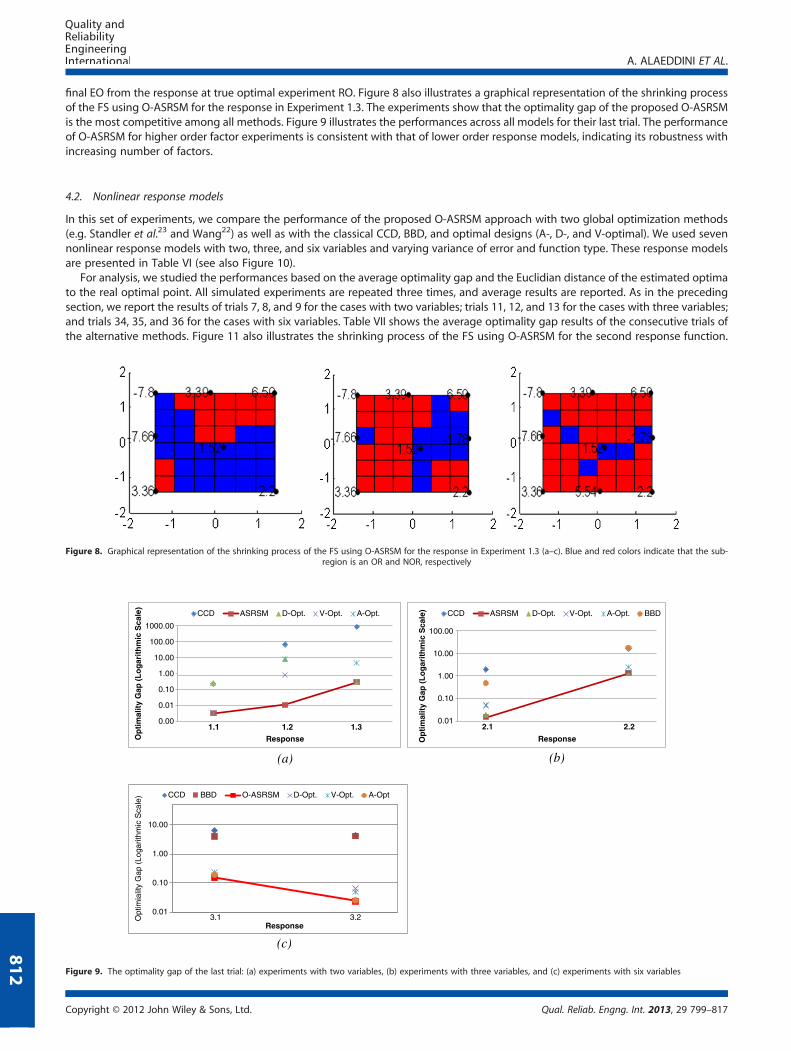
final EO from the response at true optimal experiment RO. Figure 8 also illustrates a graphical representation of the shrinking processof the FS using O-ASRSM for the response in Experiment 1.3. The experiments show that the optimality gap of the proposed O-ASRSMis the most competitive among all methods. Figure 9 illustrates the performances across all models for their last trial. The performanceof O-ASRSM for higher order factor experiments is consistent with that of lower order response models, indicating its robustness withincreasing number of factors.

4.2. Nonlinear response models

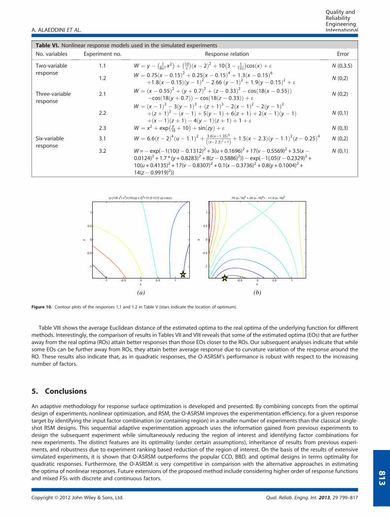
In this set of experiments, we compare the performance of the proposed O-ASRSM approach with two global optimization methods(e.g. Standler et al.23 and Wang22) as well as with the classical CCD, BBD, and optimal designs (A-, D-, and V-optimal). We used sevennonlinear response models with two, three, and six variables and varying variance of error and function type. These response modelsare presented in Table VI (see also Figure 10).

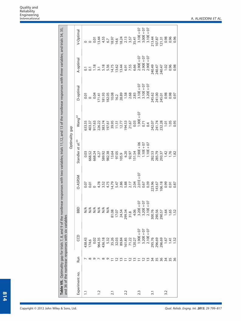
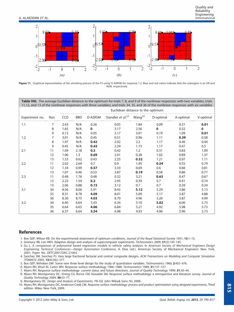
For analysis, we studied the performances based on the average optimality gap and the Euclidian distance of the estimated optimato the real optimal point. All simulated experiments are repeated three times, and average results are reported. As in the precedingsection, we report the results of trials 7, 8, and 9 for the cases with two variables; trials 11, 12, and 13 for the cases with three variables;and trials 34, 35, and 36 for the cases with six variables. Table VII shows the average optimality gap results of the consecutive trials ofthe alternative methods. Figure 11 also illustrates the shrinking process of the FS using O-ASRSM for the second response function.

0.00

0.01

0.10

1.00

10.00

100.00

1000.00

Op

tim

alit

y G

ap (

Lo

gar

ith

mic

Sca

le)

1.1 1.2 1.3Response

CCD ASRSM D-Opt. V-Opt. A-Opt.

0.01

0.10

1.00

10.00

100.00

Op

tim

alit

y G

ap (

Lo

gar

ith

mic

Sca

le)

2.1 2.2

Response

CCD ASRSM D-Opt. V-Opt. A-Opt. BBD

BBDCCD O-ASRSM D-Opt. V-Opt. A-Opt

(a) (b)

0.01

0.10

1.00

10.00

Opt

imia

lity

Gap

(Lo

garit

hmic

Sca

le)

3.1 3.2Response

(c)

Figure 9. The optimality gap of the last trial: (a) experiments with two variables, (b) experiments with three variables, and (c) experiments with six variables

Figure 8. Graphical representation of the shrinking process of the FS using O-ASRSM for the response in Experiment 1.3 (a–c). Blue and red colors indicate that the sub-region is an OR and NOR, respectively


(a) (b)

Figure 10. Contour plots of the responses 1.1 and 1.2 in Table V (stars indicate the location of optimum)

Table VI. Nonlinear response models used in the simulated experiments

No. variables Experiment no. Response relation Error

Two-variableresponse

1.1 W ¼ y � 18p2 x

2� �þ 10

p

� �x � 2ð Þ2 þ 10 3� 1

12p

� �cos xð Þ þ e N (0,3.5)

1.2 W ¼ 0:75 x � 0:15ð Þ2 þ 0:25 x � 0:15ð Þ4 þ 1:3 x � 0:15ð Þ6þ1:8 x � 0:15ð Þ y � 1ð Þ2 � 2:66 y � 1ð Þ2 þ 1:9 y � 0:15ð Þ2 þ e

N (0,2)

Three-variableresponse

2.1 W ¼ x � 0:55ð Þ2 þ y þ 0:7ð Þ2 þ z � 0:33ð Þ2 � cos 18 x � 0:55ð Þð Þ�cos 18 y þ 0:7ð Þð Þ � cos 18 z � 0:33ð Þð Þ þ e

N (0,2)

2.2W ¼ x � 1ð Þ3 � 3 y � 1ð Þ3 þ z þ 1ð Þ3 � 2 x � 1ð Þ2 � 2 y � 1ð Þ2

þ z þ 1ð Þ2 � x � 1ð Þ þ 5 y � 1ð Þ þ 6 z þ 1ð Þ þ 2 x � 1ð Þ y � 1ð Þþ x � 1ð Þ z þ 1ð Þ � 4 y � 1ð Þ z þ 1ð Þ þ 1þ e

N (0,1)

2.3 W ¼ x2 þ exp y10 þ 10� �þ sin zyð Þ þ e N (0,3)

Six-variableresponse

3.1 W ¼ 6:6 t � 2ð Þ4 u� 1:1ð Þ2 þ 3:6 v�1:35ð Þ6x�2:3ð Þ2þ1ð Þ þ 1:5 x � 2:3ð Þ y � 1:1ð Þ2 z � 0:25ð Þ4 N (0,2)

3.2 W=� exp(�1(10(t� 0.1312)2 + 3(u+ 0.1696)2 + 17(v� 0.5569)2 + 3.5(x�0.0124)2 + 1.7 * (y+ 0.8283)2 + 8(z� 0.5886)2))� exp(�1(.05(t� 0.2329)2 +10(u+ 0.4135)2 + 17(v� 0.8307)2 + 0.1(x� 0.3736)2 + 0.8(y+0.1004)2 +14(z� 0.9919)2))

N (0,1)

A. ALAEDDINI ET AL.

Table VIII shows the average Euclidean distance of the estimated optima to the real optima of the underlying function for differentmethods. Interestingly, the comparison of results in Tables VII and VIII reveals that some of the estimated optima (EOs) that are furtheraway from the real optima (ROs) attain better responses than those EOs closer to the ROs. Our subsequent analyses indicate that whilesome EOs can be further away from ROs, they attain better average response due to curvature variation of the response around theRO. These results also indicate that, as in quadratic responses, the O-ASRSM’s performance is robust with respect to the increasingnumber of factors.

813

5. Conclusions

An adaptive methodology for response surface optimization is developed and presented. By combining concepts from the optimaldesign of experiments, nonlinear optimization, and RSM, the O-ASRSM improves the experimentation efficiency, for a given responsetarget by identifying the input factor combination (or containing region) in a smaller number of experiments than the classical single-shot RSM designs. This sequential adaptive experimentation approach uses the information gained from previous experiments todesign the subsequent experiment while simultaneously reducing the region of interest and identifying factor combinations fornew experiments. The distinct features are its optimality (under certain assumptions), inheritance of results from previous experi-ments, and robustness due to experiment ranking based reduction of the region of interest. On the basis of the results of extensivesimulated experiments, it is shown that O-ASRSM outperforms the popular CCD, BBD, and optimal designs in terms optimality forquadratic responses. Furthermore, the O-ASRSM is very competitive in comparison with the alternative approaches in estimatingthe optima of nonlinear responses. Future extensions of the proposed method include considering higher order of response functionsand mixed FSs with discrete and continuous factors.


Table

VII.Optimalitygap

fortrials7,8,an

d9ofthenonlin

earresponseswithtw

ovariab

les;trials11

,12,an

d13

ofthenonlin

earresponseswiththreevariab

les;an

dtrials34

,35,

and36

ofthenonlin

earresponseswithsixvariab

les

Optimalitygap

Experim

entno.

Run

CCD

BBD

O-ASR

SMStan

dleret

al.23

Wan

g22

D-optimal

A-optimal

V-Optimal

1.1

743

8.43

N/A

0.07

0.03

633.55

0.01

0.1

08

174.6

N/A

0.01

668.52

403.37

00.1

09

0.02

N/A

066

8.24

917.63

0.04

1.18

0.01

1.2

796

4.35

N/A

4.78

6.27

226.22

171.41

3.1

13.44

843

6.18

N/A

3.52

589.92

383.74

181.93

5.18

4.55

95.32

N/A

4.75

982.38

197.61

182.05

5.56

6.7

2.1

1135

.26

81.08

14.79

13.64

39.95

10.08

14.75

18.97

1232

.03

17.07

5.47

97.05

11.51

16.2

13.62

14.6

1389

.84

24.54

2.86

105.9

12.77

28.89

13.44

18.24

2.2

1116

1.85

299.34

5.88

6.20

194.53

1.58

6.91

2.13

1271

.22

31.8

2.17

92.97

21.67

2.68

7.55

3.57

1312

0.27

4.06

2.04

151.54

0.03

2.83

6.66

35.41

2.3

111.90

E+07

3.20

E+07

2.01

E+07

7.90

E+06

1.90

E+07

3.10

E+07

2.90

E+07

3.10

E+07

125.20

E+07

3.20

E+07

0.67

1.10

E+07

0.71

3.10

E+07

2.90

E+07

3.00

E+07

132.10

E+07

2.10

E+07

0.39

1.10

E+07

0.4

3.20

E+07

2.90

E+07

3.10

E+07

3.1

3429

5.76

300.76

223.96

282.53

242.07

245.62

240.49

213.44

3529

6.69

290.56

143.67

285.79

241.74

241.00

240.47

107.87

3629

6.69

290.57

106.18

293.37

232.28

245.01

240.47

121.31

3.2

341.67

1.64

0.99

1.42

1.01

0.98

1.02

0.98

351.41

1.65

0.91

1.76

1.05

0.98

0.96

0.96

361.52

1.52

0.87

1.82

0.95

0.97

0.98

0.96

A. ALAEDDINI ET AL.


814

(a) (b) (c)

Figure 11. Graphical representation of the shrinking process of the FS using O-ASRSM for response 1.2. Blue and red colors indicate that the subregion is an OR andNOR, respectively

Table VIII. The average Euclidian distance to the optimum for trials 7, 8, and 9 of the nonlinear responses with two variables; trials11,12, and 13 of the nonlinear responses with three variables; and trials 34, 35, and 36 of the nonlinear responses with six variables

Euclidean distance to the optimum

Experiment no. Run CCD BBD O-ASRSM Standler et al.23 Wang22 D-optimal A-optimal V-optimal

1.1 7 2.43 N/A 0.26 0.05 1.84 0.09 0.31 0.018 1.65 N/A 0 3.17 2.56 0 0.32 09 0.13 N/A 0.05 3.17 3.01 0.19 1.09 0.01

1.2 7 3.01 N/A 0.45 0.51 0.96 1.11 0.39 0.588 1.97 N/A 0.42 2.02 2.2 1.17 0.46 0.449 0.45 N/A 0.43 2.39 1.73 1.17 0.47 0.5

2.1 11 1.09 2.18 0.3 0.42 1.2 0.31 0.83 1.0912 1.06 1.3 0.69 2.01 0.38 1.02 0.89 1.3713 1.53 0.62 0.43 2.25 0.32 1.21 0.97 1.11

2.2 11 2.02 2.69 0.7 0.9 1.95 0.54 0.55 0.7912 1.34 0.99 0.57 3.33 0.69 0.6 0.66 0.8113 1.07 0.46 0.53 3.87 0.19 0.58 0.86 0.77

2.3 11 0.48 1.76 0.48 0.32 3.21 0.63 0.47 0.6712 2.23 1.59 0.2 2.95 0.39 0.7 0.41 0.7413 2.06 0.88 0.15 3.12 0.7 0.7 0.39 0.34

3.1 34 8.56 8.06 5.91 8.45 5.12 5.29 5.86 5.1335 8.31 8.78 4.09 8.01 5.09 5.17 5.87 4.8836 8.30 8.75 4.03 8.70 4.96 5.20 5.87 4.99

3.2 34 6.40 6.64 5.43 6.34 5.10 5.02 6.00 5.7335 6.64 6.63 4.06 6.84 5.21 4.92 5.98 5.7336 6.37 6.64 3.54 6.98 4.93 4.96 5.96 5.73

A. ALAEDDINI ET AL.

815

References1. Box GEP, Wilson KB. On the experimental attainment of optimum conditions. Journal of the Royal Statistical Society 1951; 13:1–15.2. Gramacy RB, Lee HKH. Adaptive design and analysis of supercomputer experiments. Technometics 2009; 51(2):130–145.3. Gu L. A comparison of polynomial based regression models in vehicle safety analysis. In American Society of Mechanical Engineers Design

Engineering Technical Conferences—Design Automation Conference, A. Diaz (ed.). American Society of Mechanical Engineers: New York,2001; Paper No. DETC2001/DAC-21063.

4. Sanchez SM, Sanchez PJ. Very large fractional factorial and central composite designs. ACM Transactions on Modeling and Computer Simulation(TOMACS) 2005; 15(4):362–377.

5. Box GEP, Behnken DW. Some new three level design for the study of quantitative variables. Technometrics 1960; 2:455–476.6. Myers RH, Khuri AI, Carter WH. Response surface methodology 1966–1988. Technometrics 1989; 31:137–157.7. Myers RH. Response surface methodology- current status and future directions. Journal of Quality Technology 1999; 31:30–44.8. Myers RH, Montgomery DC, Vining CG, Borror CM, Kowalski SM. Response surface methodology: a retrospective and literature survey. Journal of

Quality Technology 2004; 36:53–77.9. Montgomery DC. Design and Analysis of Experiments, 7th Ed. John Wiley& Sons: NJ, 2008.10. Myers RH, Montgomery DC, Anderson-Cook CM. Response surface methodology: process and product optimization using designed experiments, Third

edition. Wiley: New York, 2009.


A. ALAEDDINI ET AL.

816

11. Box GEP. Statistics as a catalyst to learning by scientific method: Part II – A discussion. Journal of Quality Technology 1999; 31(1):16–29.12. Box GEP. Evolutionary operation: A method for increasing industrial productivity. Applied Statistics 1957; 6:81–101.13. Box GEP, Draper NR. Evolutionary operation: A method for increasing industrial productivity. John Wiley and Sons: NY, 1969.14. Spendley GR, Hex GR, Himsworth FR. Sequential application of simplex designs in optimization and evolutionary operation. Technometrics 1962;

4:441–461.15. Friedman M, Savage LJ. Planning experiments seeking maxima. In Techniques of Statistical Analysis, C. Eisenhart, M. Hastay, W. A. Wallis (eds.).

McGraw-Hill: NY, 1947; 363–72.16. 0Box GEP, Hunter WG, Hunter JS. Statistics for experimenters: design, innovation, and discovery, 2nd Edition. Wiley Series in Probability and Mathematical

Statistics: NY, 2005.17. Czitrom V. One-factor-at-a-time versus designed experiments. The American Statistician 1999; 53(2):126–131.18. Frey DD, Engelhardt F, Greitzer EM. A Role for one factor at a time experimentation in parameter design. Research in Engineering Design 2003;

14:65–74.19. Frey DD, Jugulum R. The mechanisms by which adaptive one-factor-at-a-time experimentation leads to improvement. American Society of Mechanical

Engineers Journal of Mechanical Design 2006; 128:1050–1060.20. Frey DD, Wang H. Adaptive one-factor-at-a-time experimentation and expected value of improvement. Technometrics 2006; 48(3):418–31.21. Wang G, Dong Z, Aitchison P. Adaptive response surface method - a global optimization scheme for computation-intensive design problems.

Journal of Engineering Optimization 2001; 33(6):707–734.22. Wang G. Adaptive response surface method using inherited Latin hypercube designs. American Society of Mechanical Engineers Journal of Mechanical

Design 2003; 125(2):210–220.23. Standler N. The Successive response surface method applied to sheet-metal forming. Proceedings of the First MIT Conference on Computationa Fluid

and Solid Mechanics, Boston, June 12–14, 2001. Elsevier Science Ltd.: Oxford, 2001.24. Moore AW, Schneider JM, Boyan J, Lee MS. Q2: A memory based active learning algorithm for black box noisy optimization. Proceedings of the

Fifteenth International Conference on Machine Learning. Morgan Kaufmann, 1998; 386–394.25. Anderson BS, Moore AW, Cohn D. A non-parametric approach to noisy and costly optimization. Proceedings of the Seventeenth International

Conference on Machine Learning (ICML), Santa Clara, CA, USA, 2000.26. Alaeddini A, Yang K., Murat A. ASRSM: A Sequential Experimental Design for Response Surface Optimization. Quality and Reliability Engineering

International 2012; To appear. DOI: 10.1002/qre.1306.27. Sobieszczanski-Sobieski J. Optimization by decomposition: a step from hierarchic to nonhierarchic systems. Second NASA/Air Force Symposium on

Recent Advances in Multidisciplinary Analysis and Optimization, Hampton, VA, NASA CP-3031, Part 1. Also NASA TM-101494, 1988.28. Renaud JE, Gabriele GA. Approximation in non-hierarchic system optimization. American Institute of Aeronautics and Astronautics Journal 1994; 32

(1):198–205.29. Rodriguez JF, Renaud JE, Watson LT. Convergence of trust region augmented Lagrangian methods using variable fidelity approximation data.

Structural and Multidisciplinary Optimization 1998; 15:141–156.30. Jones DR, Schonlau M, Welch WJ. Efficient global optimization of expensive black-box functions. Journal of Global Optimization 1998; 13:455–492.31. Alexandrov NM, Dennis JE, Lewis RM, Torczon V. A trust-region framework for managing the use of approximation models in optimization.

Structural and Multidisciplinary Optimization 1998; 15(1):16–23.32. Chang K-H, Hong J, Wan H. Stochastic trust-region response-surface method (STRONG) -- a new response-surface framework for simulation

optimization. INFORMS Journal on Computing 2012; To appear.33. Gano SE, Renaud JE. Variable fidelity optimization using a Kriging based scaling function. 10th AIAA/ISSMO Multidisciplinary Analysis and Optimization

Conference, Albany, New York, 2004.34. Rodriguez JF, Perez VM, Padmanabhan D, Renaud JE. Sequential approximate optimization using variable fidelity response surface approximations.

Structural Optimization 2001; 22(1):24–34.35. Baumert S, Smith RL. Pure random search for noisy objective functions, University of Michigan Technical Report, 2001.36. Jones DR. A taxonomy of global optimization methods based on response surfaces. Journal of Global Optimization 2001; 21(4):345–383.37. Sobieszczanski-Sobieski J, Haftka RT. Multidisciplinary aerospace design optimization: survey of recent developments. Structural and Multidisciplinary

Optimization 1997; 14(1):1–23.38. Kleijnen JPC. Design and Analysis of Simulation Experiments. Springer: New York, 2008.39. Kleijnen JPC, Van Beers WCM, Van Nieuwenhuyse I. Constrained optimization in simulation: A novel approach. European Journal of Operational

Research 2010; 202(1):164–174.40. Simpson TW, Booker AJ, Ghosh D, Giunta AA, Koch PN, Yang RJ. Approximation methods in multidisciplinary analysis and optimization: a panel

discussion. Structural and Multidisciplinary Optimization 2004; 27(5):302–313.41. Chen VCP, Tsui KL, Barton RR, Meckesheimer M. A review on design, modeling and applications of computer experiments. IIE Transactions 2006;

38:273–291.42. Kiefer J. Optimum Experimental Designs. Journal of Royal Statistical Society B 1959; 21:272–304.43. Kiefer J. Optimum Designs in Regression Problems. Annals of Mathematical Statistics 1961; 32:298–325.44. Kiefer J., Wolfowitz J. Optimum Designs in Regression Problems. Annals of Mathematical Statistics 1959; 30:271–294.45. Atkinson AC, Donev AN, Tobias RD. Optimum experimental designs with SAS. Oxford University Press: Oxford, UK, 2007; 511+xvi. ISBN: 978-0-19-929660-6.46. Pukelsheim F. Optimal Design of Experiments. Society for Industrial and Applied Mathematics (SIAM): Philadelphia, PA, 2006.47. Andere-Rendon J, Montgomery DC, Rollier DA. Design of mixture experiments using Bayesian D-optimality. Journal of Quality Technology 1997; 29

(4):451–463.48. Ginsburg H, Ben-Gal I. Designing experiments for robust-optimization problems: the Vs-optimality criterion. IIE Transactions 2006; 38(6):445–461.49. Ye KQ, William L, Sudianto A. Algorithmic construction of optimal symmetric Latin hypercube designs. Journal of Statistical Planning and Inferences

2000; 90:145–159.50. McKay MD, Beckman RJ, Conover, WJ. A Comparison of three methods for selecting values of input variables in the analysis of output from a

computer code. Technometrics 1979; 21(2): 239–245.51. Iman RL, Helton JC, Campbell JE. An approach to sensitivity analysis of computer models, Part 1. Introduction, input variable selection and

preliminary variable assessment. Journal of Quality Technology 1981; 13(3):174–183.52. Tang B. Orthogonal array-based Latin hypercube. Journal of the American Statistical Association 1993; 88(424); Theory and Methods: 1392–1397.53. Park JS. Optimal Latin-hypercube designs for computer experiments. Journal of Statistical Planning Inference 1994; 39:95–111.54. Taguchi G, Yokoyama Y, Wu Y. Taguchi methods: design of experiments. American Supplier Institute: Allen Park, Michigan, 1993.55. Owen A. Orthogonal arrays for computer experiments, integration, and visualization. Statistica Sinica 1992; 2:439–452.56. Seber GAF, Alan JL. Linear Regression Analysis. Wiley Interscience: NJ, 2003.


A. ALAEDDINI ET AL.

Authors' biographies

Dr. Adel Alaeddini is a Post Doctoral Scholar in the Department of Industrial and Operations Engineering at the University ofMichigan-Ann Arbor. His research interests include Statistical Modelling, Global Optimization, and Healthcare Operations Management.

Dr. Alper Murat is an Assistant Professor in the Department of Industrial and Systems Engineering at Wayne State University, Detroit,Michigan. Dr. Murat’s research interests include Supply Chain Management, Product Development, Healthcare Systems Engineering,and Data Mining.

Dr. Kai Yang is a Professor in the Department of Industrial and Systems Engineering at Wayne State University, Detroit, Michigan.Dr. Yang’s field of expertise includes Quality and Reliability Engineering and Management, Healthcare Systems Engineering, andProduct Development.

Dr. Bruce Ankenman is an Associate Professor in the Department of Industrial Engineering & Management Sciences at NorthwesternUniversity, Evanston, IL. Dr. Ankenman’s field of expertise includes Statistical Design of Industrial and Simulation Experiments,Engineering Design and Development, Quality Improvement and Quality Control, and Applied Statistical Methods.


817

An Efﬁcient Adaptive Sequential Methodology for …users.iems.northwestern.edu/~bea/articles/An Efficient...An Efﬁcient Adaptive Sequential Methodology for Expensive Response Surface

Documents