An Economic Theory of Leadership Mana Komai Dissertation submitted to the Faculty of the Virginia Polytechnic Institute and State University in partial fulfillment of the requirements for the degree of Doctor of Philosophy in Economics Catherine Eckel, Chair Hans Haller Nancy Lutz Richard Ashley Lise Vesterlund May 25, 2004 Blacksburg, Virginia Keywords: Leadership, Power, Information, Efficiency , Organization Copyright 2004, Mana Komai

Welcome message from author
This document is posted to help you gain knowledge. Please leave a comment to let me know what you think about it! Share it to your friends and learn new things together.
Transcript

An Economic Theory of Leadership
Mana Komai
Dissertation submitted to the Faculty of the
Virginia Polytechnic Institute and State University
in partial fulfillment of the requirements for the degree of
Doctor of Philosophy
in
Economics
Catherine Eckel, Chair
Hans Haller
Nancy Lutz
Richard Ashley
Lise Vesterlund
May 25, 2004
Blacksburg, Virginia
Keywords: Leadership, Power, Information, Efficiency , Organization
Copyright 2004, Mana Komai
An Economic Theory of Leadership
Mana Komai
(ABSTRACT)
This dissertation develops an economic theory of leadership based on assignment of informa-tion. Common theories assume that organizations exist to reduce transaction costs by replacingimperfect markets with incomplete long term contracts that give managers the power to com-mand subordinates. This view reverses all of these premises: I study an organization in whichit is costless to transmit and process information, contracts exist in the backgound if at all,and agents are not bound to the organization. The organization is held together by economiesof scale in generating information and by the advantages of controlling access to that infor-mation. The minimalist model of organizations produces a minimalist theory of leadership:leaders have no special talent but are leaders simply because they are given exclusive access tocertain information. A single leader induces a first best outcome if his incentives are alignedwith his subordinates. If a single leader is not credible, then diluting the power of leadershipby appointing multiple informed leaders can ensure credibility and improve efficiency but cannot produce the first best. If agents are differentiated by their costs of cooperation the mostcooperative player is not necessarily the best leader. In this scenario, the ability of the groupto sustain fully cooperative outcomes may depend on the player with the least propensity tocooperate. Therefore, to maximize efficiency (i.e., to maximize the range of circumstances inwhich efficient cooperation is sustainable), the group should sometimes promote less cooperativepeople. Here, ”less cooperative” means lazy or busy rather than disagreeable. This disserta-tion also applies the idea of leadership (endorsement) to voluntary provision of public goods.I show that when the leader is unable to fully reveal his information expected contributions,ex-ante, are unambigeously higher in the leader-follower setting. That is partial revelation ofinformation induces more contribution compared to full revelation or complete information. Ialso show that if the utility functions are linear then ex-ante welfare is unambigeously higherin the presence of an informed endorser.

Acknowledgments
First, I want to thank my advisor, Catherine Eckel, for her guidance before and throughout the
entire writing process. The basic idea of this dissertation grew out of her course in experimental
economics. She introduced me to the field of experimental economics and taught me how to
develop a theory that is testable by experiments. She was always available to answer my
questions and discuss my ideas.
I thank the members of my committee, Nancy Lutz, Hans Haller, Richard Ashley and Lise
Vesterlund for their useful comments.
I thank Mark Stegeman for his insightful guidance.
I also thank Farshid Mojaver Hosseini and Djavad Salehi Isfahani who made it possible for me
to attend the graduate program at Virginia Tech.
I also want to thank Barbara Barker, Sherry Williams and Mike Cutlip for their administrative
support.
Finally, I thank my friends, Subhadip Chakrabarti, Sudipta Sarangi, Matt Parrett, Ali Alichi,
Karim Jeafarqomi, Hojjat Ghandi, Rushad Faridi, Syed Islam, Narine Badasyan, Davood Soori
and Darron Thomas for making Blacksburg a nice place to be in.
I dedicate my dissertation to my family, Tooran, Naser and Raha Komai, for their love and
support all through my life.
iii

Contents
1 Literature Review 1
1.1 Introduction . . . . . . . . . . . . . . . . . . . . . . . . . . . . . . . . . . . . . . . 1
1.2 Leadership in Business and Management . . . . . . . . . . . . . . . . . . . . . . 4
1.2.1 The Classical Approaches . . . . . . . . . . . . . . . . . . . . . . . . . . . 4
1.2.2 The Contemporary Approaches . . . . . . . . . . . . . . . . . . . . . . . . 8
1.2.3 Alternative Approaches . . . . . . . . . . . . . . . . . . . . . . . . . . . . 12
1.2.4 The New Wave Approaches . . . . . . . . . . . . . . . . . . . . . . . . . . 20
1.3 Leadership in Economics . . . . . . . . . . . . . . . . . . . . . . . . . . . . . . . . 27
2 An Economic Theory of Leadership Based on Assignment of Information 37
2.1 The Basic Setup . . . . . . . . . . . . . . . . . . . . . . . . . . . . . . . . . . . . 38
2.2 Model 1: Complete Information Scenario; Homogeneous Population . . . . . . . . 41
2.3 Model 2: Incomplete Information Scenario with a Single Leader; Homogeneous
Population . . . . . . . . . . . . . . . . . . . . . . . . . . . . . . . . . . . . . . . 43
2.4 Efficiency and the single leader . . . . . . . . . . . . . . . . . . . . . . . . . . . . 46
2.5 Model 3: Incomplete Information Scenario with Multiple Leaders; Homogeneous
Population . . . . . . . . . . . . . . . . . . . . . . . . . . . . . . . . . . . . . . . 48
2.5.1 Optimal Number of Leaders . . . . . . . . . . . . . . . . . . . . . . . . . . 51
2.6 Model 4: Incomplete Information Scenario with a Single Leader; Heterogeneous
Population . . . . . . . . . . . . . . . . . . . . . . . . . . . . . . . . . . . . . . . 53
2.6.1 Efficiency and the Choice of the Leader . . . . . . . . . . . . . . . . . . . 57
2.7 Conclusion . . . . . . . . . . . . . . . . . . . . . . . . . . . . . . . . . . . . . . . 59
iv
2.8 Appendix . . . . . . . . . . . . . . . . . . . . . . . . . . . . . . . . . . . . . . . . 61
3 Leadership in Public Good Projects 77
3.1 Model 1: Provision of Public Goods under Complete Information . . . . . . . . . 80
3.2 Model 2: Provision of Public Goods with a Single Leader . . . . . . . . . . . . . 83
3.3 Overall Contributions and the Single Leader . . . . . . . . . . . . . . . . . . . . . 87
3.4 Efficiency Improvements and the Single Leader . . . . . . . . . . . . . . . . . . . 90
3.5 Conclusion . . . . . . . . . . . . . . . . . . . . . . . . . . . . . . . . . . . . . . . 93
3.6 Appendix . . . . . . . . . . . . . . . . . . . . . . . . . . . . . . . . . . . . . . . . 94
v

Chapter 1
Literature Review
1.1 Introduction
Leadership has been long studied by political theorists and social scientists. It has, however,
generally been neglected by economists. Common theories of organizations have focused on
formal and incomplete long-term contracts that give managers the power to control their sub-
ordinates (e.g. Hart (1995) and Grossman and Hart (1986)). Such theories have produced
important insights, but miss the point that leadership is distinct from formal authority. The
reason is that many of the incentives for cooperation are difficult to modify by contracts. There-
fore, to induce cooperation managers must encourage and motivate their subordinates. This is
where leadership comes into the picture.
I distinguish leadership from formal authority. This dissertation is organized in three chap-
ters. The first chapter gathers the literature on leadership in management and economics.
Leadership has been widely studied in management in various contexts and from many dif-
ferent aspects. This variety along with the informal style of management scholars makes this
literature confusing and hard to understand from an economist’s perspective. Unlike in man-
agement, leadership has not been highly recognized in economics. The purpose of chapter one
is to show the potential for economic research on leadership. It is time for economists to take
action toward formalizing this concept.
In the second chapter, I develop a minimalist model of leadership based on assignment of
information. The model, while representing only one dimension of organizations, can replicate
1

several stylized facts about organizational forms and behavior. My model does not fall into the
contract design literature mentioned above. Contracts are external to the model and appear
only implicitly in the exogenous payoffs that agents receive. The model does raise interesting
contracts design issues, which I do not answer. In my model, an organization is held together
only by economies of scale in generating information and by the advantages of restricting access
to that information. Leaders have no special talent but are leaders simply because they are
given exclusive access to certain information. I consider an organization in which leaders are
exogenously informed about the quality of the project undertaken by the organization and
decide whether to participate in the project. Leaders’ participation is observable by their
followers and serves as a signal which partially transmits their information. The binary nature
of the decision does not allow the leaders to fully reveal their information even if they want to.
Followers rely on this partial information to make their decision.
My model turns on the observation that leaders are able to use their informational advantage
to solve cooperation and coordination problems by sending a vague signal which partly reveals
their information to their followers. Uninformed followers are more cooperative, because they
do not know when their cooperative actions actually produce high personal pay-off. They rely
on the imperfect inferences that they draw from an informed leader’s actions. Leaders are also
more cooperative in the presence of ill informed agents, because their effort transmits part of
their information to the others.
In a homogeneous setting, I show that a single leader often induces cooperation, coordination
and the unconstrained first best if he can not credibly reveal all of his information. In contrast
the standard free-riding and coordination problems usually preclude first-best efficiency if all
agents are informed.
To induce cooperation and coordination, a leader should convince his followers that he is
not misleading them by transmitting incorrect information. A powerless leader will be recog-
nized and won’t be followed by his followers. In this case, diluting the power of leadership by
appointing multiple informed leaders can improve efficiency but cannot achieve the first best.
I also consider a scenario where agents are differentiated by their cost of cooperation. Relax-
ing the homogeneity assumption is not only more realistic but also allows us to address the issue
of leadership selection. In the new setting we can focus on players’ characteristics to identify the
2

optimal leader. I argue that If agents are differentiated by their costs of cooperation, then the
ability of the group to sustain cooperative outcomes may depend on the follower whose behavior
is least cooperative. I show that it is never optimal to promote the most cooperative player to
the leadership position. To maximize efficiency (i.e., to maximize the range of circumstances in
which efficient cooperation is sustainable), the group should often choose an average player. If
the average player is not powerful, it improves efficiency to choose the leaders from among less
cooperative (i.e. lazier or busier) players.
Chapter 3 applies the idea of leadership to the private provision of public goods. In this
chapter I develop a model in which the leader is exogenously informed about the value of the
public project. The leader makes two separate decisions: whether to endorse the project and
how much to participate. The leader’s endorsement (commitment) is costly and observable by
the other players. His amount of contribution, however, can not be verified by the others. As
in the former models, the leader is unable to credibly transmit all of his information, for his
amount of contribution is not verifiable.
The theoretical setting in this chapter is different and somewhat complementary to that
of chapter 2. One important distinction is that the new setting restricts the payoff structure
to a quasi-linear form but generalizes the participation decision by making it continuos rather
than binary. Another distinction is that unlike chapter 2, in the model of chapter 3 information
transmission is costly and the leader’s signal is unproductive.
I show that partial revelation of information by the leader increases the overall contributions
to lower return projects which can not be sufficiently financed under complete information. The
ex-post results in this chapter are weaker than those of chapter 2 because participation decisions
are continuos and the leader’s signal is not welfare increasing. That is, in some cases the ex-
post contributions to the higher return projects may be larger under complete information. I
show, however, that the leader increases the overall amount of contribution ex-ante. That is the
leader is able to increase the amount of contribution on average. Finally it is shown that when
followers’ payoff functions are linear and the return to the project is uniformly distributed,
the ex-ante welfare is higher under partial revelation than that of full revelation or complete
information. I also specify the conditions under which the leader increases the welfare level
ex-post.
3

1.2 Leadership in Business and Management
Leadership may be defined as the process (act) of influencing the activities of an organized
group in its efforts toward goal setting and goal achievement. (Stogdill, 1950, p. 3)
Leadership is a process of influence between a leader and those who are followers. (Hollander,
1978, p. 1)
Leadership is the behavior of an individual when he is directing the activities of a group
toward a shared goal. (Hemphill and Coons, 1957, p. 7)
The statement, ‘ a leader tries to influence other people in a given direction is relatively
simple, but it seems to capture the essence of what we mean by leadership’...(Korman, 1971,
p. 115).
As it can be seen from the above definitions, a leader is interpreted as someone who sets
direction in an effort and influences people to follow that direction.
Leadership has been long studied by business scholars but it has almost been neglected
by economists. Many of business scholars are seeking to understand and write about the
concept of leadership today. It can be confusing to try to understand leadership in business
literature, for different scholars analyze leadership in many different contexts and from many
different perspectives. There are numerous theories about leadership in business. There are
also numerous theories about leadership styles and how leaders carry out their roles.
To explore the territory of leadership in business and to investigate the potential for research
in economics, I briefly scan some of the major studies in the business literature and economics
in this chapter.
The major approaches to leadership in business and management can be classified into four
groups: Classical approaches, Contemporary approaches, Alternative approaches and the New
wave approaches.
1.2.1 The Classical Approaches
Ohio State Model, Contingency Model and Participative leadership are the most known classical
approaches in leadership literature in business and management. These theories have been
introduced initially by Schriesheim, Cogliser and Neider; Ayman, Chemers and Fiedler; and
4

Vroom and Jago, respectively. These theories are instantly recognizable by any student in
social sciences because of their resilience and longevity during the last 35 years.
Ohio State Model
The title of this section refers to a highly influential series of studies conducted by an inter-
disciplinary team of researchers. Its main impact derives from its relatively early development
of precise operational definitions of what people in leadership position do. The research team
was genuinely interdisciplinary, in that although psychologists predominated, a sociologist, an
economist, and an educationalist were also members. The focus was on the activities of leaders.
The group actually reduced this accumulation to 130 questionnaire items. This research
instrument was named the Leader Behavior Description Questionnaire (LBDQ), and was sup-
posed to reflect eight theoretical aspects of leader behavior.
A central development in the Ohio programme was a factor analysis of the results of the
administration of the LBDQ to see members of air crews, who were asked to describe the
behavior of their leaders in terms of the 130 questionnaire descriptions.
The analysis revealed that four factors predominated in the depictions of the leader behavior.
The first factor was called consideration, which denoted natural trust, liking and respect in the
relationship between leaders and their subordinates. The second factor was named initially
structure. Leaders, whose behavioral descriptions result in their receiving high scores on this
dimension tend to organize work tightly, to structure the work context, to provide clear-cut
definitions of role responsibility, and generally play a very active part in getting the work at hand
fully scheduled. The third factor is called production emphasis, which is regarded as indicative
of motivating the crew to greater activity by emphasizing the mission or job to be done. The
forth factor is named sensitivity, which refers to the awareness of social interrelationship and
pressures existing both inside and outside the subordinates.
The first two factors were the central ingredients of the measurement of leader’s behavior.
The other two factors, however, were recognized as being theoretically interesting, but not
capable of specification with the same degree of certainty.
The Ohio state questionnaire instruments have been developed during the time but the
general methodology of the Ohio State studies are the same. The approach is to focus upon
5

putative leaders in an organization. The questionnaires are administered to their subordinates in
order to gauge the behavior of the leaders. The questionnaires invariably compromise additional
scales to examine various aspects of the climate or morale of the work group attached to the
leaders. The scores of the respondents in each group are then aggregated to discern that leader’s
leadership profile and the general climate or moral by the group.
The cluster of the methodological procedures reflects three important characteristics, which
underpin much of the research in Ohio State Studies. First, the work group is the level of
analysis. Second, The focus is upon what have been called designated or putative leaders, that
is on individuals in supervisory positions within a broader hierarchy. Third, The Ohio State
studies seeks to relate descriptions of leadership to measures of outcome.
It is for the development of rigorous measures of leadership behavior and their catchy de-
scriptions of such behavior that the Ohio State researchers will be remembered.
Contingency Model
The contingency model of leadership effectiveness was presented in its most complete form in
Fiedler (1967) and Fiedler and Chemers (1974). The evolution of the model and the devel-
opment of its constructs covers three decades of research. The model predicts that a leader’s
effectiveness is based on two main factors: A leader’s attributes, referred to as task or re-
lationship motivational orientation (formerly referred to as style), and a leader’s situational
control (formerly referred to as situational favorability). The model predicts that leaders who
have a task motivational orientation compared to those, who have a relationship orientation or
motivation will be more successful in high and low control situations (Fiedler, 1987).
The model is, by design, multi-level and multi-source. That is, measures of the leader’s
motivational orientation are based on the leader’s responses (individual level); Characteristics
of the situation have been measured by the leader’s report and/or that of subordinates and ex-
perimenters (multi-level and multi-source), and outcomes have been assessed at the group level,
primarily group performance (Fiedler, 1978) as determined by objective measures, supervisor
ratings and average follower satisfaction (Rice, 1981).
The model has been the target of numerous criticism through its evolution and has been an
impetus for over 200 empirical studies. The result have supported the model .
6

Participative Leadership
How much influence a leader should permit his subordinates over matters relating to their jobs
is an important decision that all leaders face. This is the fundamental issue, which underpins
the widespread interest in how participative a leader should be, that is, how far he should allow
subordinates to determine how the work, for which he is responsible should be done; how closely
he should supervise them; and how far he should take their views into account.
An example of an approach to the study of the leadership behavior, which focuses suc-
cessively on participative leadership is the influential framework adopted by Tannenbaum and
Schmidt (1958). The title of their work was ” How to choose a leadership pattern’. In fact
the framework is about how to choose a participative leadership pattern, as the article is ef-
fectively about what degree of participation ought to be allowed to subordinates and under
what circumstances. They conceptualize the range of leadership behaviors as a continuum with
boss-centered leadership and subordinate-centered leadership as the two poles.
Participative leadership, involves a shift away from authoritarian, highly directive forms of
leadership towards a broader range of individuals being allowed and encouraged to play a part
in decision-making. The idea that greater participation must be encouraged in contemporary
organizations is widespread in the literature. Social scientists have always been at the fore-
front of the advocacy of participative management. Mulder (1971, p. 31) calls it ’the most
vital organizational problem of our time’, while Preston and Post (1974) refer to participative
management as the ’third managerial revolution’. Anthony (1978, pp. 27-9) cites eight possi-
ble advantages of participatory leadership: greater readiness to accept change, more peaceful
manager-subordinate relations, greater trust in management, increased employee commitment
to the organization, greater ease in the management of the subordinates, improved quality of
management decisions, improved upward communication and improved teamwork.
Other benefits of participation are often mentioned in the literature: for example, under
participative management people identify more with a decision and often see themselves as
having an investment in it; participation leads to a better understanding of the organization;
it enhances people’s self development; and so on.
Potential disadvantages are often mentioned in the literature on participation: it may bring
conflict to the open to such a degree that the organization falters; it may lead to time consuming
7
decisions and possibly ones, which are based too much on compromise; managers may be riddled
with anxiety if they are faced with being responsible for large numbers of decisions with which
they have little agreement; and so on.
One of the difficulties inherent in reviewing the literature on participation is simply that
researchers differ in what they mean by it. In consequence it is necessary to adopt a loose
definition of what is in any case an imprecise concept.
The research can be grouped into three main headings: experimental studies in non-
organizational settings, field experimental studies in organizations, and correlational studies
in organizations.
The reviews of relevant literature and studies show disparate findings. While, there is a
fair amount of evidence to suggest that participation contributes to satisfaction, as well as
performance, there is too much unsupporting evidence to be too confident. We can name two
factors that account for these discrepancies. Firstly, the studies reviewed cover a variety of
different types of participation, so that a failure to take into account the diversity of forms of
participation and their relative effects has contributed to a field in which comparisons between
different investigations are not always entirely sensible. Secondly, it has been recognized that
participative leadership outcome relationships are likely to be situationally contingent. The
failure to take such contextual factors into account may on occasions have led to the various
discrepancies. Because of the disparate findings, and the fuzzy implications of many of the
studies, the area of participation is a confusing one.
1.2.2 The Contemporary Approaches
The contemporary approaches have a more explicit focus on both of the leaders and the devel-
opment of their followers. This subtle shift can be seen in the three leading papers in this area.
Klein’s and House’s charismatic leadership, Avolio’s and Bass’s transformational leadership and
LMX approach of Graen and Uhl-Bien are examples the contemporary approaches.
Charismatic Leadership
Charismatic leadership has its root in political science and sociology but it can apply to or-
ganizational charisma. Charisma is a fire that ignites followers’ energy, commitment and per-
8

formance. Charisma resides not in the leader, nor a follower, but in the relationship between a
leader, who has charismatic qualities and a follower who is open to charisma, within a charisma-
conductive environment.
Charismatic leadership theory and research considers charisma to be the product of three
elements. A leader who has charismatic qualities, followers, who are open and susceptible to
charisma and an environment conductive to charisma.
(a) Leaders
Charismatic leadership theory has identified a number of personal characteristics and be-
haviors that distinguish leaders who have the potential to ignite a fire of charisma within their
subordinates. These personal characteristics include for example, prosocial assertiveness, self
confidence, need for social influence, moral conviction, and concern for the moral exercise of
power (e.g., Bass, 1988; Conger & Kanungo, 1988; House et al., 1991; House et al., 1994).
The charismatic behaviors also include articulation of distal ideological goals, communication
of high expectations and confidence in followers, emphasis on symbolic and expressive aspects
of the task, articulation of a visionary mission that is discrepant from the status quo, references
to the collective and the collective identity, and assumption of personal risk and sacrifices (e.g.,
Bass, 1985; Conger & Kanungo, 1987; House et al., 1994; Shamir et al., 1993).
It is common, within the literature on charismatic leadership, to suggest that the personal
characteristics and behaviors listed above make a leader charismatic or distinguish charismatic
leaders. But as mentioned before, the leaders characteristics and behaviors are necessary but
not sufficient to ignite charisma within subordinates. Followers and the environment also are
other important factors that are necessary to form charismatic relationships.
(b) Followers
To form charismatic relationships, subordinates also have to be open or susceptible to
charisma. Some literature suggest that the followers who are most open to charisma are vul-
nerable and/ or looking for direction or psychological meaning in life (Conger & Kanungo,
1988).
Another view suggests that the followers in charismatic relationships are not weak but are
instead compatible and comfortable with their leader’s vision and style (Shamir et al., 1993).
The third view suggests, implicitly, that followers in charismatic relationships do not differ
9

significantly from followers involved in other, non charismatic relationships. The tacit assump-
tion appears to be the leaders with charismatic qualities are so compelling and persuasive that
all followers, regardless of their personal characteristics, readily fall under these leaders’ influ-
ence. The characteristics of followers within charismatic relationships have not been investigated
empirically and therefore is ripe for empirical study.
(c) The Charisma-Conductive Environment
Some theorists argue that charismatic relationships are facilitated in the time of crises (e.g.,
Bass, 1985; Burns, 1978, Conger & Kanungo, 1988; House 1977; Weber, 1947). In crises,
individuals are uncertain and stressed and, thus, open to the influence of persuasive leaders
who offer an inspiring vision of the crisis resolved.
Charismatic leadership scholars also suggest that a variety of environmental conditions,
which simply arouse uncertainty but do not constitute real crises, may help the development
of charismatic leadership. Shamir and his colleagues (1993), argued that the emergence of
charismatic relationship is facilitated in work settings in which performance goals can not be
easily specified and measured, extrinsic rewards can not be made clearly contingent on individual
performance, and/ or there are few situational cues, constrains and reinforcers to guide behavior
and provide incentives for specific performance.
The environmental conditions conductive to charisma have received more theoretical atten-
tion than the follower characteristics, but no greater empirical attention.
As we have emphasized, according to the charismatic leadership theory, charisma resides in
the relationship of a follower and a leader and is the product of the leader, the follower and
the situation. This conceptualization is the core of charismatic leadership theory and has been
used as a stepping stone to new insights in charismatic leadership literature. A dynamic theory
of charismatic leadership is yet to be developed and Issues such as socialized and personalized
charismatic leaders, susceptible followers, Homogeneity of charisma, and its determinants and
consequences await further theoretical and empirical developments.
Transformational Leadership
The concept of transformational leadership was introduced by Bass (1985) and Burns (1978)
as distinct from other categories of leadership in that transformational leaders empower their
10

followers and encourage them to do more than they originally expected to do. Transformational
leaders were further described as having vision and as inspiring trust and respect in subordi-
nates. For the past decade, this view of leadership has become a central notion in the study of
leadership and has revitalized leadership research.
Bass (1985) examined transformational leadership through his development of the multi
factor leadership questionnaire (MLQ). The first version of MLQ included three factors, whose
joint influence was described as creating the special effect of the transformational leader:
(1)Charisma; (2) individual consideration; (3) intellectual stimulation. In a later version of
MLQ (Bass and Avolio), the factor of charisma was divided into two parts: idealized influence
and inspirational motivation. The revised MLQ thus includes four factors of transformational
leadership that measure the following influences of the transformational leader: (1) idealized
influence is defined with respect to both the leader’s behavior and the followers attributions
about the leader. Idealized leaders consider the needs of the others before their own personal
needs, avoid the use of power for personal gain, demonstrate high moral standards, and set
the challenging goals for their followers. Jointly, these behaviors set the leaders as role models
for their followers; (2) inspirational motivation refers to the ways by which transformational
leaders motivate and inspire those around them, mostly by providing meaning and challenge.
Specifically they do so by displaying enthusiasm and optimism, by involving the followers in
envisioning attractive future status, by communicating high expectations, and by demonstrat-
ing commitment to the shared goals; (3) Individualized consideration represents the leader’s
consistent effort to treat each individual as a special person and to act as a mentor, who devel-
ops his or her followers’ potential; (4) intellectual stimulation represents the leader’s effort to
stimulate the followers to be innovative and creative as well as the leader’s effort to encourage
followers to question assumptions and to reframe problems and approach them in new ways.
A large body of research portrays the transformational leader as different from, and some-
times obtaining superior outcomes to, those of other leadership styles. The focus of transforma-
tional leadership has created renewed interest in the question of what predisposes a person to
become a transformational leader and has motivated a large number of personality configuration
literature.
11

Leader-Member Exchange
The leader-member exchange approach focuses solely on (leader-follower) relationships or link-
ages. This is an extremely important clarification of the LMX approach. The leader per se
and the followers per se are not of interest in this approach. The primary variable (LMX)
in Graen’s and Uhl- Bien’s papers is defined as involving mutual trust, reciprocal trust, and
mutual obligation.
This new definition helps explain why the LMX approach, unlike the other approaches, is
not specific about the appropriate level of analysis for followers or leaders.
An essential premise of leader-member exchange theory is that leaders and supervisors
have limited amounts of personal, social, and organizational resources (e.g., time, energy, role,
discretion and positional power) and thus distribute such resources among their subordinates
selectively (e.g., Dansereau, Graen & Haga, 1975; Graen & Scandura, 1987; Graen & Uhl-Bien,
1995). Leaders do not interact with all subordinates equally, which, overtime results in the
formation of LMXs that vary in quality. Interactions in higher-quality LMXs are characterized
by increased levels of information exchange, mutual support, informal influence, trust, and
greater negotiating latitude and input in decisions. Lower-quality LMXs are characterized by
more formal supervision, less support, and less trust and attention from the leader.
The LMX theory has enhanced our understanding of the leadership communication process
between superiors and subordinates. Some research explain how the quality of LMX affect
subordinates’ and superior’s communication in areas such as discourse patterns, upward influ-
ence, communication expectations, cooperative communication, perceived organizational justice
and decision-making practices (e.g., Fairhurst, 1993; Fairhurst & Chandler, 1989; Jablin, 1987;
Krone, 1992; Lee, 1997,2001). LMX theory, however, is still open to questions and further
developments.
1.2.3 Alternative Approaches
The ideas of information processing, the substitutes for leadership approach and romance
of leadership, are grouped separated from classic or contemporary views in the alternative
category.
12
Information processing
During the past four decades there has been a trend for management practitioners and I/O
psychologists to apply information processing principles to develop theory and improve man-
agement or personnel practice. Much information processing research can be characterized in
terms of one of four general models, which provide a guiding, often implicit framework for
research. These models are labeled rational, limited capacity, expert, and cybernetic models of
information processing and behavior. Although these models are not distinguished clearly, it is
useful to view these models as different information processing perspective or metatheories.
Rational models assume that people thoroughly process all relevant information in order to
maximize relevant outcome. Traditionally, rational models dominated management science and
economic theory. The general evaluation of rational information processing models is that they
are strong in two respects. They have stimulated very explicit theories in a wide range of areas,
and their analytic basis and extensive use of information makes them prescriptively useful. The
two main deficiencies are that they usually are not descriptively accurate, nor do they generate
applications that people can apply easily. Instead, applications consistent with rational models
often require explicit instruction and the use of formal procedures or informational aids such
as computers. Thus, although rational models are appropriate in some situations and they can
be followed by people, they do not provide a very general explanation of human behavior.
In contrast to rational models, limited capacity models focus on how people simplify informa-
tion processing while still generating adequate but not optimal behaviors. These explanations
of human behavior require only limited amounts and limited processing of information. Inter-
est in these models stems from recognition of human information processing limitations. Many
studies document that human choices and behaviors do not agree with predictions from rational
models. One of the simplest and most influential limited capacity models is the satisfying model
proposed by Simon (1955). Rather than assuming exhaustive processing, this model assumes
that processing stops when the first acceptable alternative is identified. Management science
theorists similarly have characterized organizations as adaptively or boundedly rational (Cyert
& March, 1963; March & Simon, 1958). Limited capacity models do not require extensive
knowledge or omniscience, as do rational models. Instead, people work within a very limited
conceptualization of problems, considering only a few of all possible alternatives. Thus, limited
13
capacity models are more congruent with short-term memory capacities than rational models
because they require the use of less information at one time and simpler evaluation procedures.
Limited capacity models emphasize the role of cognitive heuristics and simplifying knowledge
structures in reducing information processing demands. Unlike the conscious use of algorithms
characteristic of rational models, heuristics are used informally and often without awareness.
Limited capacity models apply to leadership behavior ratings (Mitchell, Larson & Green ,
1977), Leadership perceptions (Lord, Foti & De Vader, 1984), categorization in performance
appraisal (Feldman, 1981), biases in social perceptions (Nisbett & Ross, 1980), and strategic
decision making (Brief & Downey, 1983; Dutton & Jackson, 1987). This evaluation of limited
capacity models shows that they have almost opposite strengths and Weaknesses of rational
models. Thus, limited capacity and rational models are often seen as contrasting perspectives.
The strengths of the limited capacity models are that they describe typical information pro-
cessing in many situations, provide a cognitively simple model for applications, and stimulate
new theories in several areas. However, the perspective value is weak because the model recog-
nizes that typical human information processing does not always lead to optimal decisions or
solutions.
The recognition that expertise supplements simplified information processing defines a set
of models, which are labeled expert information processing . The key assumption underlying
these models is that people rely on already developed knowledge structures to supplement
simplified means of processing information. However, these knowledge structures pertain only
to a specific content domain. Thus, an expert is defined as someone with a large knowledge
base in a particular context. For example, chess masters have approximately 50,000 chunks, or
familiar chess patterns, in memory (Simon, 1987).
A growing body of literature indicates that experts and novices differ in the way that
schema are structured. Several studies illustrate that experts and novices also differ in the
way information is processed. Experts recall of information is less biased, and they focus
more on inconsistencies in the stimulus material than novices (Fiske, Kinder, & Larter, 1983).
Generalizing this model of the human information processor, this literature suggests that experts
store and retrieve information from long term memory differently than novices (Glaser, 1982).
Experts knowledge structures in long term memory are larger and more easily accessed from
14
short term memory. In this sense, extensive knowledge substitutes for limits processing capacity
in short term memory. Put concretely, experts often recognize immediately what novices require
great effort to discover. However, it should be stressed that experts are not superior information
processors in a general sense; rather they perform better only within their specific domain of
expertise.
One primary difference between experts and novices is the greater knowledge base that
experts acquire through experience in a specific domain (Glaser, 1984). Abelson and Black
(1986) suggested that individuals with experience in familiar contexts have different knowledge
structures than those unfamiliar with the context. Therefore, they can apply different problem
solving strategies. Experts recognize relevant categories more quickly than do novices, and these
categories are linked more strongly to appropriate actions. Novices tend to organize knowledge
around literal objects and surface features explicit in a given problem statement. Experts on the
other hand, possess schema derived from knowledge of the subject matter. These schema are or-
ganized around principles that subsume the literal objects (Glaser, 1984, 1988). Moreover, when
experts identify a principle, it is connected in memory to applications of the principle. Thus
as Glaser (1988) noted, the organization of experts’ knowledge structures efficiently translates
problem information into problem solutions. In this sense, heuristic processing under expert
information processing models is something to be developed, not overcome, as it is in limited
capacity models.
Chi, Glaser, and Farr (1988) emphasized the interaction between knowledge structures and
the processes of reasoning and problem solving. They explained that experts achieve a high
level of competence because their organized body of conceptual and procedural knowledge can
be accessed and integrated with superior monitoring and self regulatory skills.
Being relatively new, expert models have not generated extensive theory in the management
area and the perspective value of such models is unexplored in the management literature.
However, recent development in using expert systems suggest that it may be high. Moreover,
work in artificial intelligence indicates that many problems, which can not be solved merely
by extensive computer processing can be solved quickly by incorporating the content specific
knowledge of experts. Work in artificial intelligence has emphasized knowledge based strategies
for the last decade. The major draw back of these models is that becoming an expert often
15

takes years of intensive study or experience. Thus, the descriptive value of expert models are
limited to career-oriented jobs, skilled trades, jobs with low turnover, or social situations that
are very common. Similarly, applications based on expert models may be very difficult for
non-expert to use due to their lack of necessary knowledge structures in long-term memory. It
is not yet known whether the acquisition of knowledge structures can be accelerated by specific
training techniques, but the issue is certainly important for the training area.
The final set of information processing models is more dynamic than the previous three.
Hogarth (1981) criticized much of the judgement and decision-making literature for focusing
on discrete events, particularly since much human judgment involves continuous adaptation
to complex and changing environments. Similarly, Ostrom argued that action is integral to
cognitive processes (1984, p. 26). Such criticism supports the use of cybernetic models, which
represent information processing and actions as being interspersed over time.
Cybernetic information processing models are dynamic, whereas all three previous mod-
els are static. In cybernetic models, behavior, learning, and the nature of cognitive processes
themselves may be altered by feedback. Also cybernetic models have future, present and retro-
spective orientations. The interpretation of past task or social information is intermixed over
time with planning future activities and executing current behaviors. The prior models adopt
a single time perspective, which may be either prospective or retrospective.
Like rational models, cybernetic models may be optimized in the long run, but they do this
by learning and adaptation, rather than by sophisticated processing before choice or behavior.
Further, as noted by Hogarth, many of the heuristic processes, which seem suboptimal for
discrete choices may be functional in a continuous environment. Hogarth (1981) argued that a
dynamic perspective provides an alternative definition of rationality based on an evolutionary
adaptation rather than the stable optimization procedures of rational economic models discussed
earlier.
Kleinmuntz and Thomas (1987) compared action oriented (cybernetic) to judgment oriented
(rational) decision strategies in a dynamic medical decision making task. They found that most
subjects used a judgement oriented strategy, which was enhanced by the provision of a rational
decision making aid. However, they also found that under conditions of low risk, the best
judgement oriented subjects barely reached the performance levels of a random, action oriented
16

benchmark procedure. Thus, decision procedures, which seem inefficient in static environments
may be very effective when choices can be repeated.
Another advantage of cybernetic models is that they are as applicable to learning as they
are to the generation of behavior. Cybernetic models, which can be traced to the early work of
Ashby (1956) and Wiener (1954), have been applied in several areas. Cybernetic information
processing characterizes models of problem recognition in which information about performance
levels is compared to some relevant standard as a means to identify problems. Cybernetic models
also apply to social perceptions in general (Hastie & Park, 1986), leadership perceptions (Lord
& Mahr, 1989b), and performance appraisal (DeNisi & Williams, 1988). Such models posit
that social perceptions are periodically reformulated by updating past perceptions with current
behavioral information. When such updating occurs, general impressions are stored in long-term
memory, but specific behavioral information is lost. Finally, cybernetic information processing
is reflected in control theory models of behavior (Carver & Scheier, 1982; Powers, 1973) and
motivation (Lord & Hanges, 1987).
The current evaluation of the cybernetic information processing models places them high in
terms of stimulating theory and in terms of both descriptive and prescriptive value. However,
it should be remembered that cybernetic models can not be used effectively when feedback is
slow or when courses of actions are costly to reverse. In terms of generating applications that fit
typical information processing, such applications require accurate, fast, and frequent feedback.
If these conditions are present, people should find applications based on cybernetic models easy
to use.
Substitutes for Leadership
The idea of substitutes for leadership was formulated most explicitly by Kerr and Jermier
(1978) to draw attention to the possibility that many of the situational factors, which moderate
leadership-outcome relationships do so by tending to negate the leader’s ability to either improve
or impair subordinate satisfaction or performance. This can occur because particular situational
factors neutralize the effects of leadership style. Kerr and Jermier distinguish between two
general types of leader behavioral: Relationship-oriented/supportive/people-centered leadership
and task oriented/instrumental/job-centered leadership.
17

According to Kerr and Jermier, substitutes for leadership can best be grouped into three
headings: subordinate, task, and organizational characteristics. They argue that different sub-
stitutes tend to neutralize the effects of different leadership styles. They report a study of city
police in which the relative effects of the substitutes and both instrumental and supportive
leader behavior were examined to discern their relative impact on police officers’ organizational
commitment and role ambiguity. They found that the impact of leader behavior on these two
outcome variables was small. They also find that few of the substitutes had a strong effect on
the outcomes, which renders an interpretation of the lack of influence of the leader behaviors
somewhat indeterminate.
A very similar study was conducted on hospital employees by Howell and Dorfman (1981)
using the same leader behavior and substitutes scales. The two outcome variables investigated
were organizational commitment and job satisfaction. They find out that a leader’s supportive
behavior will make a difference to organizational commitment and job satisfaction and substi-
tutes do not negate such leader behavior.
Finally, Podsakoff et al. (1984) also investigated the impact of the substitutes for leadership
scales on the effect of different reward and punishment behaviors. In this investigation, very
little evidence was found for the substitutes for leadership approach.
Kerr and Jemrmier’s approach is interesting but it seems that the first tranche of results is
not too encouraging. It may be that a concentration of a wider range of leader behaviors and
substitutes in relation to each other will bear fruit.
Romance of leadership
The romance of leadership notion (introduced by Meindle, Ehrlich & Dukerich, 1985) refers
to the prominence of leaders and leadership in the way organizational actors and observers
address organizational issues and problems, revealing a potential bias or false assumption-
making regarding the relative importance of leadership factors to the functioning of groups and
organizations.
The romance of leadership emphasizes leadership as a social construction. Attention is
focused on development of theory and hypothesis regarding the features, outcomes, and im-
plications of the social construction process, as it occurs among followers and as it is affected
18

by the contexts in which they are embedded. It seeks to understand the existence of general
and more situation-specific concepts of leaders and how they are conceptualized and otherwise
constructed by actors and observers.
Although there are currently many available perspectives that highlight the thoughts and
phenomenology of the leader, the romance of the leadership is about the thoughts of follow-
ers: how leaders are constructed and represented in their thought systems. The romance of
leadership perspective focuses on the linkage between leaders and followers as constructed in
the minds of followers. Rather than assuming leaders and followers are linked in a substan-
tially casual way, it assumes that the relationship between leaders and followers is primarily a
constructed one, heavily influenced by interfollower factors and relationships. The behavioral
linkages between the leader and follower are seen as a derivative of the constructions made by
followers. The behavior of followers is assumed to be much less under the control and influence
of forces that govern the social construction process itself.
One aspect of a leader-centric perspective is a focus on the persona of the leader. The
romance of leadership perspective moves a researcher away from the personality of the leader
as a significant substantive and casual force on the thoughts and actions of followers. It instead
places more weight on the images of leaders that followers construct for one another. It assumes
that followers react to, and are more influenced by, their constructions of the leader’s personality
than they are by the true personality of the leader. It is the personalities of leaders as imagined
or constructed by followers that become the object of study, not actual or clinical personalities
per se.
Similarly, this approach does not explain or deal with the behavior of the leader and the
direct impact of that behavior on followers. In other words, direct effects of the actions and
activities of the leader, independent of and unmoderated or unmediated by social construction
processes, are not addressed. Thus, leadership is assumed to be revealed not in the actions or
exertions of the leader but as part of the way actors experience organizational processes. In
essence, leadership is very much in the eyes of the beholder: followers not the leader define it.
From this perspective, the idea that leadership can not and does not occur without followers is
taken literally to be true.
The leader centric perspective favors the rather direct control of followers by engaging in
19

so called leadership behaviors. The present approach would emphasize more indirect and less
tightly controlled effects on followers. Manipulations of contexts and constructions, rather
than of leader behaviors, would in a sense, constitute the practice of leadership. Rather than
searching for the right personality, one would search for the opportunity to create the right
impression. Reputations would be more significant than actions. Rather than being concerned
about engaging in the right practices, one would be concerned about creating the right spin.
The creation and sustenance of the interpretive dominance regarding leadership would have the
highest priority.
Those who have aspirations for an objective theory of leadership will find great difficulty
with the inherently subjectivistic, social constructionist view being advanced here. A subjective
definition and a social construction view of leadership does not imply that it can not be studied
through normal scientific processes of inquiry. Meindle shows it is possible to use the romance
of leadership notion, with its constructionistic, followership-centric bent to formulate testable
hypotheses. There are likely many existing possibilities for research at all levels of analysis, the
only real limitation being the creativity and the interest of the researcher.
1.2.4 The New Wave Approaches
Self leadership, Multiple-Linkage Model, Multi level theory and Individualized leadership can
be categorized in the new wave approaches in leadership literature.
Self Leadership
Self leadership literature pays attention to a neglected aspect of organizational behavior- the
influence organization members exert over themselves. This managerial focus has emerged pri-
marily from the social learning theory literature (Bandura, 1969; Cautela, 1969; Goldfried and
Merbaum, 1973; Kanfer, 1970; Manhoney and Arnkoff, 1978, 1979; Manhoney & Thoresen,
1974). In the organization literature, this process generally has been referred to as self man-
agement (Andrasik & Heimberg, 1982; Luthans & Davis, 1979; Manz and Sims, 1980; Marx,
1982; Mills, 1983).
Organizations impose multiple controls of varying character on employees. One view sug-
gests that the control process involves applying rational, manageable, central mechanisms to
20
influence employees through external means to assure that the organization achieves its goals.
An alternative view, however, shifts the perspective of the control system-controlee inter-
face significantly. Self leadership perspective, views each person as possessing an internal self
control system (Manz, 1979). Organizational control systems in their most basic form provide
performance standards, evaluation mechanisms, and systems of reward and punishment. Sim-
ilarly, individuals posses self generated personal standards, engage in self evaluation processes
and self administrative rewards and punishments in managing their daily activities (Bandura,
1977a, Mahoney and Thoresen, 1974; Manz and Sims, 1980). Even though these mechanisms
take place frequently in an almost automatic manner, this makes them no less powerful.
Further more, while organizations provide employees with certain values and beliefs pack-
aged into cultures, corporate visions and so forth, people too possess their own systems of values,
beliefs, and visions for their future. In addition, the counterparts of organization rules, policies,
and operating procedures are represented internally in the form of behavioral and psychological
scripts or programs held at various levels of abstraction.
The point is organizations provide organizational control systems that influence people but
these systems do not access individual actions directly. Rather, the impact of organizational
control mechanisms is determined by the way they influence, in intended as well as unintended
ways, the self control systems within organization members.
While this perspective is not new, an analysis of theory and research in the field reveals that
it has not been well integrated into organizational management. The literature does include
cognitive mediation of external stimuli (e.g. social learning theory views- Davis & Luthans,
1980; Manz & Sims, 1980) and attributed causes to observed physical actions (Feldman, 1981;
Green & Mitchell, 1979; Mitchell & Larson & Green, 1977; Staw, 1975) but does not adequately
recognize the self-influence system as a focal point for enhanced understanding and practice
of organizational management. This perspective, on the other hand, suggests that the self
influence system is the ultimate system of control. In addition, it suggests that this internal
control system must receive significant attention in its own right before maximum benefits for
the organization and employee are realized.
Recent work on cybernetic (control) theory provides a useful perspective for making concrete
the nature of employee self-regulating systems (Carver & Scheier, 1981, 1982). Carver and
21
Scheier (1981) present an insightful view of the self regulating process involving : (a) input
perceptions of existing conditions, (b) comparison of the perception with an existing reference
value, (c) output behaviors to reduce discrepancies from the standard, and (d) a consequent
impact on the environment.
From this view, an employee attempting to achieve a given production standard would
operate within a closed loop of control aimed at minimizing deviations from standards in existing
performance. Unless an environmental disturbance of some kind occurred, this self regulating
process theoretically could occur indefinitely.
Carver and Scheier (1981, 1982) further speculated, based on the work of powers (1973a,
1973b), that standards emerge from a hierarchical organization of control systems. That is,
standards for a particular control system loop derive from superordinate systems of control.
Thus, an employee working to achieve a minimum deviation from a production standard at one
level may serve higher level systems aimed at higher level standards.
From an organizational perspective, recognizing and facilitating employee self regulating
systems pose a viable and more realistic view of control than views centered entirely on exter-
nal influence. In addition, overreliance on external controls can lead to number of dysfunctional
employee behaviors: Rigid bureaucratic behavior, inputting of invalid information into man-
agement information systems and so forth.
More relevant treatments of self management to date focused on strategies designed to
facilitate behaviors targeted for change (Andrasik & Heimberg, 1982; Luthans & Davis, 1979;
Manz & Sims, 1980). This work generally reflects the view that behaviors are not performed for
their intrinsic value but because of their necessity or because of what the performer will receive
for his performance. A widely recognized definition of self-control, one that illustrates this view,
is: A person displays self control when in the relative absence of immediate external constraints
he engages in behavior, whose previous probability has been less than that of alternatively
available behaviors (a less attractive behavior but one that is implied to be more desirable).
Several specific self management strategies can be identified. Mahoney and Arnkoff (1978,
1979) provided a useful array of strategies that were applied in clinical contexts. These include,
self observation, self goal setting, cueing strategies, self reinforcement, self punishment, and
rehearsal. Much of the employee self management literature has centered on adaptations of
22

these self control strategies for addressing management problems (Andrasik & Heimberg, 1982;
Luthans & Davis, 1979; Manz & Simz, 1980, 1981).
Luthans and Davis, (1979) provided descriptions of cueing strategy interventions across
a variety of work contexts. Physical cues such as a wall graph to chart progress on target
behaviors and a magnetic message board were used to self induce desired behavioral change in
specific cases. Manz and Sims (1980) explicated the relevance of the broader range of self control
strategies, especially as substitutes for formal organizational leadership. Self observation, cueing
strategies, self goal setting, self reward, self punishment, and the rehearsal were each discussed in
terms of their applicability to organizational contexts. Andrasik and Heimberg (1982) developed
a behavioral self management program for individualized self modification of targeted work
behaviors. Their approach involved pinpointing a specific behavior for change, observing the
behavior over time, developing a behavioral change plan involving self reward or some other
self influence strategy, and adjusting the plan based on self awareness of a need for change.
In terms of cybernetic self regulating systems (Carver & Scheier, 1981, 1982), these employee
self management perspectives can be viewed as providing a set of strategies that facilitate
behaviors that serve to reduce deviations from higher level reference values that the employee
may or may not have helped establish. That is, the governing standards at higher levels of
abstraction can remain largely externally defined even though lower level standards to reach the
goals may be personally created. Mills (1983) argued that factors such as the normative system
and professional norms can exercise just as much control over the individual as a mechanistic
situation in which the performance process is manipulated directly. This view is consistent with
arguments that employee self control is perhaps more an illusion than a reality (Dunbar, 1981)
and that self managed individuals are far from loosely supervised or controlled (Mills, 1983).
In addition, it has been argued that self management strategies themselves are behaviors that
require reinforcement in order to be maintained (Kerr & Sllocum, 1981; Manz & Sims, 1980;
Thoresen & Mahoney, 1974). Because of this dependence on external reinforcement, it could be
argued that the self management approach violates Thoresen and Mahoney’s (1974) definition
cited earlier, in the long run. That is, while immediate external constraints or supports may
not be required, longer-term reinforcement is.
The considerable attention devoted to individual self influence processes in organizations
23

has been focusing primarily on self management that facilitates behaviors that are not naturally
motivating and that meet externally anchored standards. Manz (1986), proposed a more com-
prehensive approach to more fully address the higher-level standards/ reasons that employee
self influence is performed and to suggest self influence strategies that allow the intrinsic value
of work to help enhance individual performance.
Further research and theoretical development is needed to address several central elements
of self influence- for example, the derivation of personal standards at multiple hierarchical levels,
human thought patterns, self influence strategies that build motivation into target behaviors-
that have been neglected in the employee self management literature.
Multiple Linkage Model
Most leadership theories deal with a few selected behaviors rather than a wide range of lead-
ership behaviors. An exception is Yukl’s (1989, 1994) multiple linkage model, which identifies
categories of leadership behavior that are relevant for most types of managerial positions. The
multiple linkage model builds on earlier theories of effective leadership behavior and theories
of effective groups. According to the model, the effects of leader behavior on work unit perfor-
mance are mediated by individual level intervening variables (subordinate effort, role clarity,
and ability) and by group level intervening variables (work organization, teamwork, resources
for doing the work and external coordination). Some of the leadership behaviors (clarifying,
delegating, developing, recognizing, supporting) are used primarily to influence the individual
level intervening variables. Other leadership behaviors (planning, problem solving, monitor-
ing, team building) are used primarily to improve group-level intervening variables. However,
there is no simple one to one correspondence between leader behaviors and the intervening
variables. Rather, effective leadership depends on the overall pattern of leader behavior and its
relevance to the situation. Situational variables (the nature of the task, the characteristics of
subordinates, and the external environment) influence the intervening variables and determine
which leadership behaviors are relevant to a particular manager. The multiple linkage model
and most prior research on leadership behavior deal with leadership effectiveness rather than
advancement.
There has been little empirical research to test the model. Although hundreds of studies
24

have been conducted in the past four decades to investigate the behavior associated with effec-
tive leadership, most of this research has examined broad categories of task oriented behavior
that are difficult to relate to the demands and challenges faced by managers in different situa-
tions. The number of studies on specific behaviors is still small, and different researchers have
examined different subsets of behaviors, making it difficult to compare results across studies.
Multi-level Theory
Some years ago, Dublin (1979) contrasted the terms leadership of organizations and leadership
in organizations in an insightful decision. Leadership of organizations is similar to what some
now term strategic leadership, it involves human actors in interaction with the organization as
an entity. Leadership in organizations involves the kind of lower organizational level, face to
face interactions that comprise more than 90 percent of the current leadership literature (Hunt,
1991; Phillips & Hunt, 1992).
Hunt’s model, which examines leadership up and down the organizational hierarchy, involves
the complex relationships of both kinds of leadership operating together. Hunt’s (1991) model
argues, first, that there are critical tasks that must be performed by leaders if an organization
is to perform effectively. Because of an assumed increasingly complex setting as one moves
higher in an organization, these critical tasks become increasingly complex and qualitatively
different. The extended model assumes that the critical tasks can be divided by organizational
levels within three domains. The bottom domain is labeled direct or production, The middle
domain is called organizational, and the top domain is labeled systems or strategic.
The number of levels encompassing critical tasks within the domains is argued to vary as a
function of the organization’s size, the time span, and the requirement that each level add value
to both its higher and its next lower level. The model argues that generally, even for the largest
organizations, the number of levels probably should not exceed seven, from the employee level
to the very top. For a large complex organization, then, there would be: (1) an employee and
two leadership levels in the production domain; (2) two leadership levels in the organizational
domain; and (3) two leadership levels in the strategic domain.
Hunt’s extended model also assumes that accompanying the increasing task complexity by
organizational level, there must be an increasing level of the leader cognitive capacity. Con-
25

sistent with requisite variety notions, there should be a rough match between leader cognitive
capacity and critical task complexity at each organizational level. The extended level also as-
sumes that there is an accompanying leader behavioral complexity notion comprised of leader
behaviors or skills. Hunt’s model also includes leader background, predisposition, value prefer-
ences, organizational culture or subculture, and various aspects of organizational and subunit
effectiveness. Finally, the organization is considered to be embedded within external environ-
ment and societal culture aspects.
Individualized leadership
The individualized leadership is introduced in a paper by Dansereau et al. This approach views
people as forming relationships with one individual totally independent of the relationships
they form with other individuals. There need to be no consistency on the part of an individual
in forming relationships with multiple individuals. That is, an individual may treat a group of
people the same way or all differently; it depends on how he or she views the other individuals.
According to this view, formal as well as informal relationships between a focal individual or a
superior and other individual (e.g. a subordinate) tell us nothing about that focal individual’s
relationship with any other individual.
In this new approach to leadership, leaders first provide support for the sense of self-worth of
followers as unique individuals, who are independent of other individuals they interact. Second,
in exchange, followers then perform in ways that satisfy the leader. Third, as a result, leaders
and followers link in dyads, where there is consistency and agreement, yet differences between,
these independent dyads.
This theory is tested in a number of studies, and nearly identical effects were found in all
studies. This approach would be enhanced by considering some of the features of other new
wave approaches. An increase in the number of variables of interest in future research seems
appropriate.
26
1.3 Leadership in Economics
The concept of leadership has not received as much attention in economics as it has in business
and management. There are some interesting economic contributions to the leadership theory
literature, however, which analyze leadership as a concept distinguished from formal authority,
namely Kreps (1990a), Rotemberg and Saloner (1993), Hermalin (1998), Vesterlund (2000), and
Andreoni (2004). Kreps, Rotemberg and Saloner begin from an incomplete contract setting,
Hermalin takes his starting point in the Holmstrom (1982) complete contracts team model and
Vesterlund and Andreoni address leadership in a charitable fund-raising context.
Strictly speaking Kreps’s paper is not about leadership per se, but rather about corporate
culture and how reputation that a corporate culture may help build provides an important part
of the explanation of firms’ organization. Nevertheless, it certainly makes provision for leader-
ship. Kreps’s paper is an explorative discussion aimed at convincing organizational economists
of the possibility of alternative routs of research. Starting from property rights/incomplete
contracts theory (Grossman and Hart, 1986; Hart, 1995), Kreps argues that incompleteness
of contracts may produce a need for implicit contracts. However, in the face of unforeseen
contingencies it is not clear how implicit contracts should be administered; in particular it is
not clear how well standard reputation arguments work with unforeseen contingencies. The
possible role of leadership in this setting is to provide general principles that instruct employees
and suppliers about how unforeseen contingencies will be handled in the future by management.
Another notable leadership theory is Julio J. Rotemberg and Garth Saloner (1993), which
studies the question of leadership styles. Rotemberg and Saloner are more taken up with
how leadership styles are influenced by environmental contingencies. However, the same ba-
sic insights as in Kreps, namely that the provision of incentives is not straight forward under
incomplete contracting, plays a key role in their paper. Rotemberg and Saloner provide an
economic model in which leadership style has an important effect on firms’ profitability. They
show that senior management’s style can alter the incentives that can be provided for subor-
dinates to ferret out profitable opportunities for the firm. Leadership style is modeled as the
degree to which the leader empathizes with followers (formally, the weight the leader’s utility
function assigns to the followers’ utility).
Rotemberg and Saloner argue that the personality of the leader affects both the management
27

style and the ease with which this incentive problem is overcome. Specifically, they study the
relationship between a firm’s environment and its optimal leadership style inside a setting, where
contracts between the firm and subordinates are incomplete so that providing incentives to
subordinates is not straightforward. Leadership style, whether based on organizational culture
or the personality of the leader, then affects the incentive contracts that can be offered to
subordinates.
Rotemberg and Saloner show that in an incomplete contracting environment, empathy can
serve as a commitment device and, therefore, be valuable. They argue that leaders who em-
pathize with their employees adopt a participatory style and that the shareholders gain from
appointing such leaders when the firm has the potential for exploiting numerous innovative
ideas. By contrast, when the environment is poor in new ideas, shareholders benefit from
hiring a more selfish (i.e., more profit maximizing) leader whose style is more autocratic.
Hermalin offers a finely honed theory about leadership behavior. He defines a leader as
someone with followers and argues that following is inherently a voluntary activity and, there-
fore, a central question in understanding leadership is how does a leader induce others to follow
him. As an economist he presumes that followers follow because it is in their interest to do
so. Hermalin argues that followers believe that leader has better information about what they
should do than they have. He believes that leadership is about transmitting information to the
followers and convincing them that he is transmitting the correct information.
Hermalin suggests two ways in which a leader can convince his followers to put in more
effort in the organizational activities. One is leader’s sacrifice: The leader offers gifts to the
followers. The followers respond not because they want the gifts themselves, but because the
leader’s sacrifice convinces them that she must truly consider this to be a worthwhile activity.
The other way to convince the followers in Hermalin’s opinion is leading by example: The
leader himself puts in long hours on the activity, thereby convincing followers that she indeed
considers it worthwhile.
He studies incentive problems in the context of the team model of Holmstrom (1982). He
argues that Bengt Holmstrom’s team model is well suited for studying leadership. First, because
the leader shares in the team’s output, she has an incentive to exaggerate the value of effort
devoted to the common activity. Second, because the information structure limits the leader’s
28

ability to coerce followers, she must induce their voluntary compliance with his wishes. As
holmstrom showed, since each person gets only a fraction of the overall return to his effort, he
expends less than the first-best level of effort on the common endeavor. In other words, he fails
to internalize the positive externality his effort has for the firm. This team problem is thus
simply an example for free riding problem endemic to the allocation of public goods.
Hermalin assumes that only one leader has information about the return to effort allocated
to the common endeavor. Given asymmetric information he considers two possible ways that the
leader can credibly communicate all of his information. First he considers a mechanism design
setting. Hermalin shows that a mechanism that makes side payments among team members
a function of the leader’s announcement about his information can duplicate the symmetric-
information second-best outcome. In the second setting Hermalin allows the leader to lead by
example, that is, he expends effort before the other workers. Based on the leader’s effort, the
other workers form beliefs about the leader’s information. He shows that leading by example
yields an outcome that is superior to the symmetric-information outcome. The reason for this
conclusion is that the hidden information problem counteracts the team problem: The need to
convince the other workers increases the leader’s incentives, so he works harder.
Hermalin, then proceeds to derive what the optimal contract (shares) should be when the
leader leads by example. He finds that in a small team, he has the smallest share, but in a
large team he has the largest share. Hermalin argues that under certain conditions, leading by
example dominates symmetric information even when attention is restricted to equal shares.
Hermalin focuses on what the leader does to induce a following. He does not consider the
questions of how the leader is chosen, why people want to be leaders or who is the best choice
for the leadership position. Hermalin’s theory also falls into the contract economics approach
as of Kreps’s, Rotemberg’s and Saloner’s works.
Vesterlund’s model investigates sequential fund-raising and the role of the fund-raiser in
fund-raising games under incomplete information. The hypothesis of her paper is that when
the information about the quality of the charity is unknown, an announcement strategy for a
high type charity is successful because it helps reveal the information about the quality of the
charity. Vesterlund’s paper assumes that the first contributor obtains costly information about
the charity’s quality. She argues that when the information cost is sufficiently low, a first mover
29
who is informed with a high signal fully reveals the value of the charity through a large initial
contribution. This increase in contribution decreases the donation of the second contributor
but the overall contribution level exceeds the complete information scenario.
Vesterlund’s model investigates sequential fund-raising and the role of the fund-raiser in
fund-raising games under incomplete information. The hypothesis of her paper is that when
the information about the quality of the charity is unknown, an announcement strategy for a
high type charity is successful because it helps reveal the information about the quality of the
charity. Vesterlund’s paper assumes that the first contributor obtains costly information about
the charity’s quality. She argues that when the information cost is sufficiently low, a first mover
who is informed with a high signal fully reveals the value of the charity through a large initial
contribution. This increase in contribution decreases the donation of the second contributor
but the overall contribution level exceeds the complete information scenario.
Andreoni develops a model of leadership giving in charitable fund-raising. His aim is to
provide a positive economic model for the observation that charitable fund-raisers often rely
on leadership givers, who are typically wealthy individuals who give exceptionally large gifts to
the charity. He argues that gifts can be a signal of the quality of the charitable good. Since the
person sending the signal would rather all followers think the quality is high, the leader must
give an exceptionally large gift for the signal of quality to be credible. He argues that the game
of providing the signal then reduces to a familiar war of attrition game where the person with
the lowest cost-benifit ratio is the one who provides the good immediately who is the wealtiest
person assuming identical preferences.
The above modelling efforts are neat, logical and produce interesting and sometimes counter-
intuitive conclusions. The basic thrust of this literature is to conceptualize virtually any issue
related to the economics of organizations in terms of solving incentive conflicts. Thus the
essence of the above contributions is that leaders exist because they resolve incentive conflicts,
albeit sophisticated and non-standard ones.
The role of leadership, however, is not limited to resolving incentive conflicts. The view
that all, or most, organizational phenomena are reducible to problems of aligning incentives is
one that is implicitly contradicted by contributions to organization studies (Thompson, 1967),
The executive and leadership literature (Barnard, 1948; Carlsson, 1951; Selznick 1957; Kotter,
30
1996), political science (Calvert,1992,1995), sociology (coleman, 1990) and in some quarters of
economics of organization (Milgrom and Roberts, 1992, Ch. 4; Camerer and Knez, 1994, 1996,
1997; Langlois, 1998; Weber, 1998; Langlois and Foss, 1999). Many of these contributions are
directly related to the issue of leadership.
For example, Coleman (1990) observes that charismatic authority may be a response to co-
ordination problems that do not necessarily turn on misaligned incentives. Camerer and Knez
(1994, 1996, 1997) and Calvert (1992, 1995) argue that attention should be shifted to coordi-
nation games (rather than cooperation games) in seeking a foundation for the understanding
of organizational phenomena.
Nicolai J. Foss (2000) provides an explorative discussion somewhat in the style of Kreps,
aimed to emphasize the importance of leadership as a way of solving the coordination problems.
He argues that all the emphasis has been on cooperation games, i.e. games where the payoff
space of the game is such that the efficient outcomes are not supportable as equilibria at least
in one-shot play. The key problem that such a game leads one to ponder is how to avoid the
Pareto-inferior outcome. Indeed the basic hold-up situation has a prisoners’ dilemma structure
and this is also the case with the team production problem and other problems with information
externalities and moral hazard.
Foss criticizes the lack of interest in the interaction problems that may be represented by
coordination games, which is in his opinion a somewhat surprising neglect given the increasing
emphasis on such problems in other areas of economics, such as standards, conventions, learning
behavior and macroeconomics.
He mostly focuses on shared interest coordination games distinct from coordination games
with mixed interests1. Foss argues that classical game theory solves the coordination problem
by defining it away, that is, by assuming that agents by means of pure ratiocination can reason
their way to equilibrium. Moreover, sometimes in classical game theory literature it is argued
that suppressing coordination problems is justified because it allows concentration on essentials.
Foss, argues that coordination games are non-trivial and quite fundamental and claims that
leadership may, in certain situations, be a low cost device to solve the problem of coordination.
1 In the shared interest coordination games players’ preferences over equilibria coincide. In contrast, coordi-nation games with mixed interests will also exibit multiple equilibria, but these equilibria are ranked differentlyby the players.
31

Foss defines leadership as the taking of actions that coordinate the complimentary actions
of many people through the creation of belief conditions that substitute for common knowledge
and where these actions characteristically consist of some act of communication directed at
those being led. He distinguishes between coordination problems in which common knowledge
about payoffs and strategies obtains initially and those in which it does not. He also makes a
distinction between games where agents can communicate by exchanging cheap talk at no or
low cost and those in which they can’t (or communication is very costly). However, the leader
will be privileged by being the only player who can always communicate if he so chooses. Foss
introduces four cases following this distinction, in which leadership plays different roles.
Case 1) This represents the case where leadership is least likely to play a role, since knowledge
is common and agents may communicate at low or no cost.
Case 2) This represents the case, where agents can not engage in communication but the
common knowledge assumption is maintained. In this case, based on substantial empirical
evidence players may not choose the efficient equilibrium. In this situation the leader may, by
playing the efficient equilibrium and making this common knowledge, induce the other players
to play the efficient equilibrium.
Case 3) This refers to the situation, where knowledge is not held in common but agents may
communicate at no or low cost. In this case if communication costs are zero, one could expect
common knowledge conditions to be established instantaneously and coordination follow in the
same split second. There may be a role for leadership if communication costs are positive.
Case 4) This represents the situation where knowledge is not held in common and agents
can not communicate. This case is the most realistic of the four cases. In this situation players
have incomplete information (or non at all) about other players, available strategies, previous
plays, etc. and games have to be redefined and played anew. In this situation there is unlikely
to be an exact correspondence between players, strategies and outcomes of the game. There
will be likely to be multiple equilibria. Foss argues that in such a situation leadership may be
conceptualized as picking one equilibrium out of a multiplicity, for establishing belief conditions
that approximate common knowledge.
Foss states that leadership may be thought of in terms of remedying: (i) problems of coor-
dinating on an equilibrium when agents are initially outside the equilibrium; (ii) problems of
32

coordinating on one equilibrium out of a multitude; (iii) problems of moving from an inferior
equilibrium to the efficient equilibrium by influencing the beliefs that agents hold.
Leadership as an institutional solution for coordination problems, has also been investigated
in experimental economics literature. Wilson and Rhodes (1997) begin their research with one
component of leadership- its coordinating role- and disentangle how leadership matters for
followers. They proceed their analysis as a simple one-sided signalling game from leaders to
followers and investigate when a leader’s signals are credible. The empirical analysis is based
on a series of laboratories experiments in which groups of four actors were involved in a series of
one stage coordination games. They show that although leadership is crucial for coordinating
followers, the introduction of uncertainty about the type of leader markedly decreases the
ameliorating impact of leadership.
Wilson and Rhodes, concentrate on three types of n-player coordination games. The first
is a pure coordination game with no leader. The second is a pure coordination game with a
leader, who produces cheap talk signals for followers. The third type is a coordination game
with an uncertain type leader. Their game has a symmetric payoff structure and therefore there
is no Pareto ranking over the Nash equilibria. In the absence of a Pareto superior alternative,
each of the equilibria is equivalent. The problem for players is to coordinate on a single choice,
a task that is not as simple as it seems.
They show that in a pure coordination game with no leader, subjects fail to coordinate
as predicted. In their second setup, full coordination is not automatic. The existence of a
credible leader, however, considerably increases the overall coordination rates. In the third
stage, Wilson and Rhodes introduce uncertainty about the types of the leaders. In other words
they induce some uncertainty about the commonality of interests between leader and follower.
From the followers standpoint a good leader’s incentives are aligned with theirs. A bad leader’s
interests, however, diverge from those of the followers. A good leader has strong incentives to
send a coordinating signal to the followers. On the other hand, a bad leader always has an
incentive to send misleading signals to his followers. In this setup the leaders are informed
about their type but followers only have probabilistic information about which kind of leader
they are facing. The results show that in non of the trials under this condition did followers
fully coordinate. They also show that in assessing leader’s suggestion, subjects are sensitive
33

not only to the presence of uncertainty but to the degree of that uncertainty. Therefore they
conclude that leadership is clearly important for resolving coordination problems. Leadership
can serve as a focal point, helping followers choose one equilibrium from among several. They
argue, however, that the only presence of leadership is no guarantee that coordination problems
will be solved. If followers are uncertain about their leader’s incentives, then they can easily
ignore leadership.
Another interesting experimental economics contribution to the leadership literature is
Vesterlund, Potters, and Sefton (2004). They examine endogenous sequencing in voluntary
contribution games when some donors do not know the true value of the good. They not only
study whether an informed leader can use her contribution to convince others of the quality of
the public good, but also whether the sequential ordering may arise endogenously. Their ex-
perimental study shows that the vast majority of subjects prefer that the informed contributor
gives first and the contribution of the informed donor be revealed to the uninformed. They
find out that the resulting contributions and earnings in these endogenously generated sequen-
tial games are much larger than those found when subjects make donations simultaneously.
When the informed player’s donation is announced, the uninformed player mimics her behavior
and the informed player correctly anticipates this response. They also compare the endoge-
nous determination of contribution orderings to the case where the ordering is set exogenously.
This result suggests that the gain from announcements is smaller when the sequence of play is
determined by an outside party.
This dissertation is different from the current leadership literature in economics in several
ways. First, unlike Kreps, Rotemberg, Saloner and Hermalin my model does not fall into
the contract design literature2. My purpose is not to disregard other important aspects of
organizations but to show that it is possible to address important questions of organizational
design while suppressing all issues of monitoring, bargaining and contracts. I also argue that
leadership is not necessarily a very complicated concept. Leaders sometimes play an important
role in achieving cooperation and coordination even if they have no special talent. In my
model the leader is simply an average player with exclusive access to information. I model an
environment in which an organization is held together simply by the advantages of controlling
2There is no question that payoffs may be affected by contracts, but this issue remains in the background.
34

access to information.
Second, In my model as of Hermalin’s and Vesterlund’s, a leader is simply an average player
who has exclusive information about the value of the project undertaken by the organization
but unlike their model the leader’s participation in the project only partially transfers his
information to his subordinates. Therefore, in my model the leader increases efficiency not
by revealing all of his information but by sending a vague signal which partially reveals the
value of the project. In my model, the first best is achieved not only because the leader works
harder to set an example for the others, but also because followers do not know exactly when
their participation yields high personal payoffs. Therefore, the employees participate to socially
efficient projects which they refuse to participate in if the value of the project is fully revealed3.
Third, while the current literature on leadership addresses incentive conflicts and coordina-
tion problems separately, I define leadership as an institutional solution to both cooperation and
coordination problems. That is, in this model a leader not only eliminates incentive conflicts
but also coordinates the group members at the same time.
The forth contribution of this paper is to address the power of leadership theoretically. I
argue that leadership is not just about information transmission. A leader should convince his
followers that he is transmitting correct information. A leader who is unable to convince his
followers is not able to induce a following and is considered to be a powerless leader. I show that
appointing multiple leaders improves the power of leadership. An organization with multiple
informed leaders can not achieve the first best but is more efficient than an organization in
which the value of the project is common knowledge. I also specify the optimal number of
leaders that maximizes efficiency.
This dissertation also addresses the issue of leadership selection by considering a heteroge-
neous structure in which the employees are differentiated by their cost of participation. I show
that it is never optimal to promote the most cooperative player to the leadership position. To
maximize efficiency, the group should often choose an average player. If the average player
is not powerful enough to induce a following it improves efficiency to choose the leaders from
among less cooperative players.
3The issue of private and social value of information and its role in designing efficient social/economic policiesand structures have also been addressed in information economics literature (Hirshleifer 1971, Stephen 2002, andArthur 1992)
35

The next chapter introduces the first four models and presents the results in more detail.
36

Chapter 2
An Economic Theory of Leadership
Based on Assignment of Information
In this chapter, I develop a minimalist theory of leadership in which leadership is formed only
based on assignment of information. This chapter introduces four models representing four
different organizational structures. First I explain the basic set up which is common in all four
models. Then as a benchmark, I consider a homogeneous organization in which all the members
are equally informed about the value of the project undertaken by the organization. The second
model represents a different organizational structure in which only one player is informed about
the value of the project and is appointed to be the only leader of the organization. The rest
of the players are uninformed followers. In the third model, I consider an organization with
multiple informed leaders who lead symmetric groups of followers. The fourth model considers
a single leader organization but relaxes the assumption of homogeneous population.
As mentioned before, this section investigates how leadership which is formed based on
information improves participation and efficiency within an organization. This analysis can
be applied to a setting where the adoption of new methods can increase a firm’s profitability.
Adoption of new methods may be everything from simple changes in the production process
to the introduction of completely new products. All of these require that employees first think
about ways to change the firm’s operations and later cooperate to implement the change. Most
large scale changes in a firm go through several stages of this kind.
37
From the firm’s point of view the generation of proposals is extremely valuable and needs to
be encouraged. One can consider a setting, where employees are supposed to start investment
projects that might lead to a change. It is not possible, however, to ensure that employees work
hard at generating viable proposals. This is an appropriate assumption whenever the activity
of proposal generation can not itself be structured and monitored. We can argue that the
outside appearance of a proposal need not bear a close relationship to the amount of effort that
went into developing it because it is hard to monitor and measure intellectual activity. This
problem arises not only in the research laboratory but also where a large number of employees
is expected to develop ideas for continuous improvement. In conclusion when a firm wants to
generate proposals for change they confront a difficult incentive problem.
Other potential applications include cooperation to win a contest or contract or political
campaigns.
The following section introduces the basic setup of our model.
2.1 The Basic Setup
In this section I construct the basic setup, which is common in all four models. I consider m
identical players, i ∈ I = {1, 2, ...,m}, who constitute an organization or otherwise benefit fromcollective action. Each player makes a discrete decision whether to join a project undertaken
by the organization. Therefore, each player’s action set is A = {P,N}, where, P denotes
participation and N stands for not participating in the project.
The quality index of the project is the random variable x, which is distributed on the
interval [0, x] with the density function φ(x). Participating in the project is costly and the cost
of participation is fixed at c > 0 for all players. Let ai ∈ A denote player i’s action and c(ai)his cost of participation. Thus c(N) = 0 and c(P ) = c.
At the beginning of the game, nature chooses x. Then some or all players observe x (ac-
cording to the model considered) and each player chooses an action ai ∈ A. I assume thatuninformed players do not participate in the project.
Player i’s payoff is γ(ai, q;x)−c(ai), where q is the fraction of the m players who participate
in the project. Assume that the function γ : A × [0, 1] × <+ → < is C2; it is economically
38
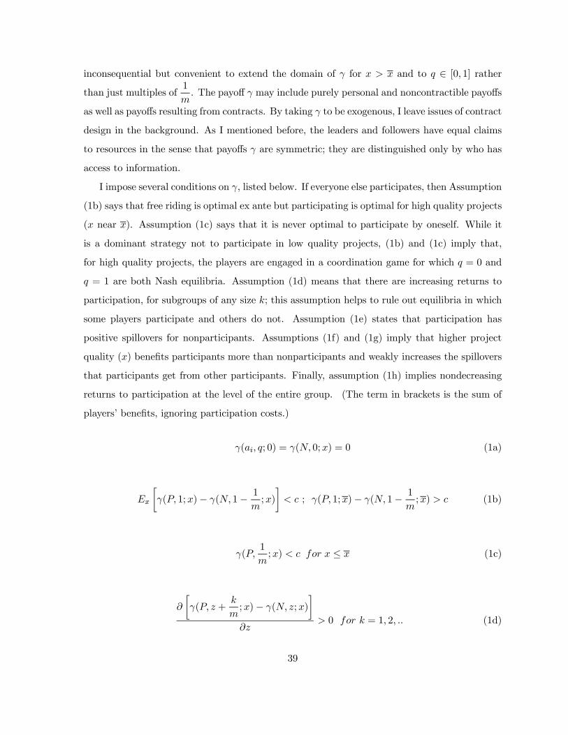
inconsequential but convenient to extend the domain of γ for x > x and to q ∈ [0, 1] ratherthan just multiples of
1
m. The payoff γ may include purely personal and noncontractible payoffs
as well as payoffs resulting from contracts. By taking γ to be exogenous, I leave issues of contract
design in the background. As I mentioned before, the leaders and followers have equal claims
to resources in the sense that payoffs γ are symmetric; they are distinguished only by who has
access to information.
I impose several conditions on γ, listed below. If everyone else participates, then Assumption
(1b) says that free riding is optimal ex ante but participating is optimal for high quality projects
(x near x). Assumption (1c) says that it is never optimal to participate by oneself. While it
is a dominant strategy not to participate in low quality projects, (1b) and (1c) imply that,
for high quality projects, the players are engaged in a coordination game for which q = 0 and
q = 1 are both Nash equilibria. Assumption (1d) means that there are increasing returns to
participation, for subgroups of any size k; this assumption helps to rule out equilibria in which
some players participate and others do not. Assumption (1e) states that participation has
positive spillovers for nonparticipants. Assumptions (1f) and (1g) imply that higher project
quality (x) benefits participants more than nonparticipants and weakly increases the spillovers
that participants get from other participants. Finally, assumption (1h) implies nondecreasing
returns to participation at the level of the entire group. (The term in brackets is the sum of
players’ benefits, ignoring participation costs.)
γ(ai, q; 0) = γ(N, 0;x) = 0 (1a)
Ex
·γ(P, 1;x)− γ(N, 1− 1
m;x)
¸< c ; γ(P, 1;x)− γ(N, 1− 1
m;x) > c (1b)
γ(P,1
m;x) < c for x ≤ x (1c)
∂
·γ(P, z +
k
m;x)− γ(N, z;x)
¸∂z
> 0 for k = 1, 2, .. (1d)
39
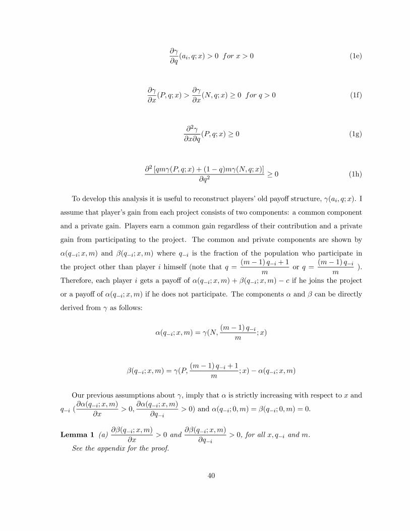
∂γ
∂q(ai, q;x) > 0 for x > 0 (1e)
∂γ
∂x(P, q;x) >
∂γ
∂x(N, q;x) ≥ 0 for q > 0 (1f)
∂2γ
∂x∂q(P, q;x) ≥ 0 (1g)
∂2 [qmγ(P, q;x) + (1− q)mγ(N, q;x)]
∂q2≥ 0 (1h)
To develop this analysis it is useful to reconstruct players’ old payoff structure, γ(ai, q;x). I
assume that player’s gain from each project consists of two components: a common component
and a private gain. Players earn a common gain regardless of their contribution and a private
gain from participating to the project. The common and private components are shown by
α(q−i;x,m) and β(q−i;x,m) where q−i is the fraction of the population who participate in
the project other than player i himself (note that q =(m− 1) q−i + 1
mor q =
(m− 1) q−im
).
Therefore, each player i gets a payoff of α(q−i;x,m) + β(q−i;x,m) − c if he joins the projector a payoff of α(q−i;x,m) if he does not participate. The components α and β can be directly
derived from γ as follows:
α(q−i;x,m) = γ(N,(m− 1) q−i
m;x)
β(q−i;x,m) = γ(P,(m− 1) q−i + 1
m;x)− α(q−i;x,m)
Our previous assumptions about γ, imply that α is strictly increasing with respect to x and
q−i (∂α(q−i;x,m)
∂x> 0,
∂α(q−i;x,m)∂q−i
> 0) and α(q−i; 0,m) = β(q−i; 0,m) = 0.
Lemma 1 (a)∂β(q−i;x,m)
∂x> 0 and
∂β(q−i;x,m)∂q−i
> 0, for all x, q−i and m.
See the appendix for the proof.
40

In the next section I introduce a model which represents a homogeneous organization in
which all members have complete information and show how under complete information an
organization is unable to achieve the first best.
2.2 Model 1: Complete Information Scenario; Homogeneous
Population
As a benchmark, I first consider the case that all players observe the project quality x and then
make simultaneous participation decisions. A player’s strategy thus takes the form s : [0, x]
→ A. Let #P and #N denote the numbers assigned to participation and non-participation
respectively. let #P ≡ 1 and #N ≡ 0 and let
Πm(si, s−i;x) ≡ γ
µsi(x),
Pj∈I #sj(x)m
;x
¶− c(si(x))
denote player i’s payoff from adopting strategy si given x and other player’s strategy s−i. A
Nash equilibrium of the game is the strategy profile S∗ = (s∗i , i ∈ I) such that:
s∗i (x) = Argmaxsi
Πm(si, s∗−i;x) ∀i ∈ I, x ∈ [0, x]
For simplicity, I restrict my attention only to symmetric equilibria such that each player
adopts a threshold strategy. A threshold strategy is x∗ such that players play P iff x > x∗.
Allowing other equilibria introduces no new phenomena of interest and just some additional
complex equilibria.
Theorem 2 Define the unique threshold τm ∈ (0, x) such that
hm(τm) = β(1; τm,m)− c = 0
The threshold strategy x∗ constitutes a Nash equilibrium iff τm ≤ x∗
See the appendix for the proof.
Theorem (2) states that in the complete information scenario, players decide not to par-
ticipate in the project for all values of x less than τm. For any value of x between τm and x
41
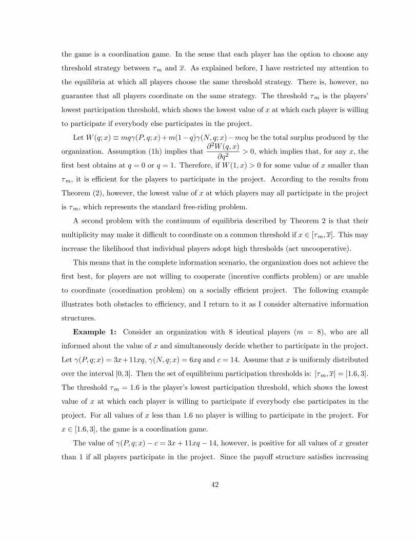
the game is a coordination game. In the sense that each player has the option to choose any
threshold strategy between τm and x. As explained before, I have restricted my attention to
the equilibria at which all players choose the same threshold strategy. There is, however, no
guarantee that all players coordinate on the same strategy. The threshold τm is the players’
lowest participation threshold, which shows the lowest value of x at which each player is willing
to participate if everybody else participates in the project.
Let W (q;x) ≡ mqγ(P, q;x)+m(1− q)γ(N, q;x)−mcq be the total surplus produced by theorganization. Assumption (1h) implies that
∂2W (q, x)
∂q2> 0, which implies that, for any x, the
first best obtains at q = 0 or q = 1. Therefore, if W (1, x) > 0 for some value of x smaller than
τm, it is efficient for the players to participate in the project. According to the results from
Theorem (2), however, the lowest value of x at which players may all participate in the project
is τm, which represents the standard free-riding problem.
A second problem with the continuum of equilibria described by Theorem 2 is that their
multiplicity may make it difficult to coordinate on a common threshold if x ∈ [τm, x]. This mayincrease the likelihood that individual players adopt high thresholds (act uncooperative).
This means that in the complete information scenario, the organization does not achieve the
first best, for players are not willing to cooperate (incentive conflicts problem) or are unable
to coordinate (coordination problem) on a socially efficient project. The following example
illustrates both obstacles to efficiency, and I return to it as I consider alternative information
structures.
Example 1: Consider an organization with 8 identical players (m = 8), who are all
informed about the value of x and simultaneously decide whether to participate in the project.
Let γ(P, q;x) = 3x+11xq, γ(N, q;x) = 6xq and c = 14. Assume that x is uniformly distributed
over the interval [0, 3]. Then the set of equilibrium participation thresholds is: [τm, x] = [1.6, 3].
The threshold τm = 1.6 is the player’s lowest participation threshold, which shows the lowest
value of x at which each player is willing to participate if everybody else participates in the
project. For all values of x less than 1.6 no player is willing to participate in the project. For
x ∈ [1.6, 3], the game is a coordination game.The value of γ(P, q;x)− c = 3x+ 11xq − 14, however, is positive for all values of x greater
than 1 if all players participate in the project. Since the payoff structure satisfies increasing
42

returns to participation at the level of the entire group, the efficient outcome is for all players
to participate in the project for all values of x ∈ (1, 3], which is not supported by any of theequilibria in the game. The conclusion is: in the complete information scenario, the organization
does not achieve the first best.
In the next section I show that the standard coordination and cooperation problems can be
solved by appointing a single leader, who has exclusive access to information and is unable to
fully transmit his information to the others.
2.3 Model 2: Incomplete Information Scenario with a Single
Leader; Homogeneous Population
This section pursues the idea that, even if it is costless, as in model 1, to make information about
the project quality available to all players, it may improve efficiency to select one player arbi-
trarily and give her exclusive access to that information (e.g., the output of the organization’s
research department). In other words, it may improve efficiency to reduce player’s access to
information artificially. It is implicit in this approach that the excluded players cannot discover
x for themselves, perhaps because that would be too costly for an individual.
I revise the model by changing (only) the timing and the information structure. I assume
that exactly one player l ∈ I observes x (the leader) and that the leader acts first choosingal ∈ A. Then the remaining followers observe the leader’s action and act simultaneously. LetF ≡ I\{l} denote the set of followers.
In this extensive game, the leader’s strategy takes the form sl : [0, x]→ A and each follower’s
strategy takes the form sF : A → A. Note that the leader cannot report x to the followers,
even if she wishes to. The interpretation is that the leader typically benefits by reporting a
false (e.g., high) value of x, and the followers are unable to verify the leader’s report. Each
follower’s four possible strategies can be abbreviated SF = {PP,NN,C,R}, where the strategyPP means that follower f always participates, NN means that follower f never participates, C
means that the follower always copies the leader’s action and R means always reject the leader’s
43

actions. Let
Π1(sl, s−l;x) ≡ γ
µsl(x),
#sl(x) +Pi∈F #si(sl(x))m
;x
¶− c(sl(x))
denote the leader’s payoff as a function of all players’ strategies, and similarly for each follower
f ∈ F :
Π1(sf , s−f ;x) ≡ γ
µsf (sl(x)),
#sl(x) +Pi∈F #si(sl(x))m
;x
¶− c(sf (sl(x)))
Let χ be a measurable subset of [0, x] and µ(χ) = prob(x ∈ χ). Given sl(x), define χP =
{x ∈ [o, x] : sl(x) = P} and χN = {x ∈ [o, x] : sl(x) = N}. A Perfect Bayesian equilibrium of
the game is the strategy profile S∗ = (s∗l , s∗f ) and the posterior beliefs µ(χ | χP ) and µ(χ | χN)
such that:
s∗l (x) = Argmaxsl
Π1(sl, s∗−l;x) ∀x ∈ [0, x]
s∗f (al) = Argmaxsf
Ex[Π1(sf , s∗−f ;x) | s∗l (x) = al]
∀al ∈ A such that al occurs with positive probability given s∗l , ∀f ∈ F.
µ(χ | χP ) =µ(χ)µ(χP | χ)
µ(χP )
µ(χ | χN ) =µ(χ)µ(χN | χ)
µ(χN)
The three following lemmas and theorem help us characterize the equilibrium. Lemma 3
simplifies the followers’ gain from participation. Lemma 4 shows that all followers copy the
leader in any nontrivial equilibrium which implies that the leader leads by example. Finally,
Theorem 5 characterizes the equilibria.
Lemma 3 Followers’ expected gain from participation conditional on the leader’s action, de-
pends only on their conditional expected private gain, E[β(q−i;x,m) | al, sl].See the appendix for the proof.
Lemma 4 If (s∗l ; s∗f , f ∈ F ) is an equilibrium strategy profile such that the leader participates
with positive probability, then s∗f = C for all f ∈ F .See the appendix for the proof.
44

The idea behind Lemma 4 is that the equilibrium participation of any one leader or follower
implies, by increasing returns to participation (assumption (1d)), that others should also par-
ticipate. Followers should not participate unconditionally, however, because the ex ante returns
are too low (assumption (1b)). The only remaining possibility is for followers to copy the leader.
If the leader adopts a threshold strategy x∗, then the followers learn from his action either
that x ≤ x∗ or x > x∗. If x∗ is too small, then the leader asks too much and the followers
become unwilling to follow. In this case, we say that the leader has no power. The following
theorem shows the existence of an equilibrium in which the leader is powerful and is able to
induce a following.
Theorem 5 Define the unique thresholds τ1 ∈ (0, x), τF ∈ (0, x), such that
h1(τ1) = α(1; τ1,m) + β(1; τ1,m)− c = 0
br(τF ) = Ex[β(1;x,m) | x ≥ τF ]− c = 0
Then, the pair (x∗, s∗f , f ∈ F ) is a positive participation equilibrium iff x∗ = τ1 (τF < τ1) and
s∗f = C for all f ∈ F .See the appendix for the proof.
The presence of a single informed leader greatly reduces the number of equilibria. The
above theorem characterizes those equilibria. There always exists a trivial no-participation
equilibrium, with the leader choosing the threshold strategy x∗ = x (i.e., she never participates)
and the followers all choosing NN . Aside from such trivial equilibria, there exists at most
one positive-participation equilibrium, meaning that the probability that at least one player
participates exceeds zero.
Lets explain the positive-participation equilibrium in more detail. The threshold τ1 repre-
sents the leader’s optimal strategy given that all followers play C. If τ1 < τF , then the signal
conveyed by his participation decision (i.e., x > x∗) is too weak to convince the followers to
participate: they would expect her to participate too often in circumstances that they would
not find individually advantageous. Therefore, equilibrium participation requires satisfaction
45
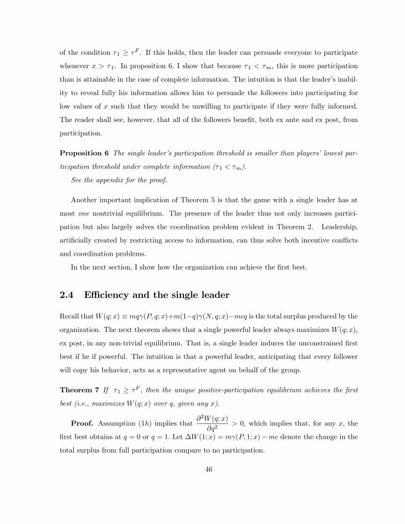
of the condition τ1 ≥ τF . If this holds, then the leader can persuade everyone to participate
whenever x > τ1. In proposition 6, I show that because τ1 < τm, this is more participation
than is attainable in the case of complete information. The intuition is that the leader’s inabil-
ity to reveal fully his information allows him to persuade the followers into participating for
low values of x such that they would be unwilling to participate if they were fully informed.
The reader shall see, however, that all of the followers benefit, both ex ante and ex post, from
participation.
Proposition 6 The single leader’s participation threshold is smaller than players’ lowest par-
ticipation threshold under complete information (τ1 < τm).
See the appendix for the proof.
Another important implication of Theorem 5 is that the game with a single leader has at
most one nontrivial equilibrium. The presence of the leader thus not only increases partici-
pation but also largely solves the coordination problem evident in Theorem 2. Leadership,
artificially created by restricting access to information, can thus solve both incentive conflicts
and coordination problems.
In the next section, I show how the organization can achieve the first best.
2.4 Efficiency and the single leader
Recall thatW (q;x) ≡ mqγ(P, q;x)+m(1−q)γ(N, q;x)−mcq is the total surplus produced by theorganization. The next theorem shows that a single powerful leader always maximizes W (q;x),
ex post, in any non-trivial equilibrium. That is, a single leader induces the unconstrained first
best if he if powerful. The intuition is that a powerful leader, anticipating that every follower
will copy his behavior, acts as a representative agent on behalf of the group.
Theorem 7 If τ1 ≥ τF , then the unique positive-participation equilibrium achieves the first
best (i.e., maximizes W (q;x) over q, given any x).
Proof. Assumption (1h) implies that∂2W (q;x)
∂q2> 0, which implies that, for any x, the
first best obtains at q = 0 or q = 1. Let ∆W (1;x) = mγ(P, 1;x)−mc denote the change in thetotal surplus from full participation compare to no participation.
46

By assumption∂W (1;x)
∂x=
∂γ(P, 1;x)
∂x> 0.
By definition of τ1 and since∂W (1;x)
∂x> 0 we can conclude that ∆W (1;x) > 0 for all
x > τ1 and ∆W (1;x) < 0 for all x < τ1. Therefore, full participation (q = 1) is efficient for all
x > τ1 and q = 0 is efficient for all x < τ1.
Therefore, since τ1 > τF , the existence of the positive participation equilibrium from The-
orem (6) implies that a single leader can induce a first best outcome.
Example 2: Consider the organization introduced in Example 1. Now, however, assume
that exactly one player is promoted to the leadership position and allowed to observe x. The
leader is powerful because τ1 = 1 exceeds τF = 0.2. Therefore, a positive participation equi-
librium exists. In this equilibrium, the leader participates only for x ≥ 1 and is followed byeveryone else.
If the leader is not powerful because the condition (τ1 > τF ) is not satisfied, he won’t be
able to induce a first best outcome simply because he will not be followed by his subordinates.
There are several potential ways to increase the power of the leader (short of redesigning the
payoff structure γ). One way is to relax the assumption that the population is homogeneous.
Considering a heterogeneous organization is not only more realistic, but also allows us to focus
on the players’ characteristics to choose the most appropriate person for the leadership position,
who is powerful and able to create the highest surplus (This scenario will be discussed in model
4). It will be shown that if some players have high participation costs, then appointing a lazy
or busy (high cost) player to the leadership position can increase the power of leadership.
Another way to increase the power of leadership is to appoint multiple informed leaders
in the organizational structure. This increases each leader’s power by reducing each leader’s
influence. I show that multiple leadership can restore the power of leaders by increasing their
participation threshold above τF .
It will be shown that the total surplus in the multi-leader scenario is higher than the complete
information scenario, but multiple leadership can not induce the unconstrained first best. The
multi-leader scenario is interesting but it raises the question of how leaders can coordinate
on participation. This creates an incentive for future research. Considering a hierarchical
organization and appointing a top leader followed by subleaders may solve the coordination
problem among the subleaders. This idea is undeveloped at this stage but it may bear fruit in
47

the future.
Next section analyzes how multiple leadership affects the power of leadership and the equi-
librium outcome of the game. It also addresses the question of what is the optimal number of
leaders that maximizes the total surplus produced by the organization.
2.5 Model 3: Incomplete Information Scenario with Multiple
Leaders; Homogeneous Population
This section considers the same model of leadership, with one difference. I now allow multiple
players to lead identically sized groups of followers. Let L ⊂ I denote the set of leaders
and F (l) ⊂ I the set of followers of leader l ∈ L. I assume that each follower has only oneleader and no followers; L and F (l)l∈L thus constitute a partition of I. Let n ≡ #L ∈ N(m)denote the number of leaders, where N(m) ≡ {1, ...m} denotes the integer factors of m, and letrn ≡ m
n− 1 denote the number of followers per leader. It is economically reasonable to allow
n to take integer values n /∈ N(m), but my formal analysis does not accommodate fractionalfollowers.
I show that multiple leaders can be powerful and induce participation in circumstances such
that a single leader could not persuade anyone to participate. Unlike a single leader, multiple
leaders generally cannot induce first best outcomes ex ante, but I derive the number of leaders
needed to support the constrained optimum.
The model of multiple leaders may be appropriate for political or other contexts in which
numerous groups work together toward a common objective. The leader of a single large group
might have too many followers to be powerful (because he gets a large payoff from his followers’
participation and therefore he has a greater incentive to exaggerate the value of the project),
but smaller groups can cooperate effectively if their leaders can solve the coordination problem
among themselves.
Consider the following extensive game, similar to the game of the previous section. Nature
initially chooses x, the leaders observe x, and then each leader l ∈ L chooses an action al ∈ A.After the leaders act simultaneously, each follower f ∈ F (l) observes leader l’s action andchooses an action af ∈ A. The followers act simultaneously. As before, a leader’s strategy is
48

a function sl : [0, x] → A, and a follower’s strategy is a function sf : A → A. The followers’
strategies can again be represented by the set SF = {PP,NN,C,R}. Let
Πn(si, s−i;x) ≡ π
si(sl(x)),Pl∈Lh#sl(x) +
Pf∈F (l)#sf (sl(x))
im
;x
− c(si(sl(x)))denote the payoff to follower i ∈ F (l), as a function of all players’ strategies. If player i is theleader, then the formula is the same except that si(x) replaces si(sl(x)).
To simplify matters, I consider only group symmetric equilibria, meaning that each group
adopts a strategy profile identical to that of each other group. If the followers adopt diverse
strategies, then the proportion of followers who adopt a given strategy is the same in each
group.
Recall that χ is a measurable subset of [0, x] and µ(χ) = prob(x ∈ χ). Given sl(x), I also
defined χP = {x ∈ [o, x] : sl(x) = P} and χN = {x ∈ [o, x] : sl(x) = N}. A Perfect Bayesian
equilibrium of the game is the strategy profile S∗ = (s∗l ; s∗f , f ∈ F (l)) and the posterior beliefs
µ(χ | χP ) and µ(χ | χN) such that:
s∗l (x) = Argmaxsl
Πn(sl, s∗−l;x) ∀x ∈ [0, x]
s∗f (al) = Argmaxsf
Ex[Πn(sf , s∗−f ;x) | s∗l (x) = al]
∀al ∈ A such that al occurs with positive probability given s∗l , ∀f ∈ F (l)
µ(χ | χP ) =µ(χ)µ(χP | χ)
µ(χP )
µ(χ | χN) =µ(χ)µ(χN | χ)
µ(χN )
As for the other models, assumption (1c) implies that the multi-leader case always supports
a no-participation equilibrium (e.g. leaders never participate and every follower plays NN). If
leaders participate with positive probability, however, then I can show, as in the case of a single
leader, that followers must copy their leaders in equilibrium.
Lemma 8 If (s∗l ; s∗f , f ∈ F (l)) is a group symmetric equilibrium such that leaders participate
with positive probability, then s∗f = C for all f ∈ F (l).See the appendix for the proof.
49

As in the complete information setting of Model 1, but not the single leader setting of Model
2, the presence of multiple informed players introduces coordination problems that support
complicated equilibria incorporating non-threshold strategies. To simplify matters somewhat,
I follow the pattern of Model 1 by restricting attention to threshold strategies for the informed
players. The following theorem, generalizes Theorems 2 and 5 from the extreme cases n = m
(i.e. complete information) and n = 1 to intermediate numbers of leaders.
Theorem 9 Define the unique thresholds τAn ∈ (0, x), τBn > τAn , τF ∈ (0, x), such that
hAn (τAn ) = α(1; τAn ,m) + β(1; τAn ,m)− α(
m³1− rn
m
´− 1
m− 1 ; τAn ,m)− c = 0
hBn (τBn ) = α(
rnm− 1; τ
Bn ,m) + β(
rnm− 1; τ
Bn ,m)− c = 0
br(τF ) = Ex[β(1;x,m) | x ≥ τF ]− c = 0
Then, the pair (x∗; s∗f , f ∈ F (l)) is a positive participation group symmetric equilibrium iff
Max©τAn , τ
Fª ≤ x∗ ≤ τBn and s
∗f = C.
See the appendix for the proof.
Theorem 9 shows that the presence of multiple leaders complicates the determination of
equilibrium, because the leaders’ participation threshold is not unique; the leaders play a coor-
dination game among themselves, in which the (symmetric) equilibrium participation threshold
can fall anywhere in the interval [τAn , τBn ]. The threshold τAn is the lowest value of x at which a
leader is willing to participate if all other leaders are also willing to participate. The threshold
τBn is the lowest value of x for which a leader is willing to participate even if no other leader
participates. For n = 1 the interval [τAn , τBn ] collapses to the point τ1.
Theorem 9 shows that the power constraint for n leaders, analogous to the τ1 ≥ τF condition
for one leader, is τBn ≥ τF . Proposition 10 shows that increasing the number of leaders relaxes
this constraint.
Proposition 10 If n0> n then τA
n0 > τAn and τB
n0 > τBn .
50
See the appendix for the proof.
As mentioned before, the above proposition shows that the leaders’ participation threshold
increases with the number of leaders. Therefore appointing more leaders can improve leaders’
power.
As the reader can see, the participation interval in the multi-leader case (Max©τAn , τ
Fª ≤
x∗ ≤ τBn ) captures smaller values of x, relative to the complete information scenario (τm ≤x∗ ≤ x), because τm > τAn . This means that the total surplus is higher in the multi-leader case.
2.5.1 Optimal Number of Leaders
Theorem 9 and Proposition 10 suggest that the optimal number of leaders is whatever value
of n ∈ N(m) that is just large enough to create a powerful leader (τBn ≥ τF ). Fewer leaders
cannot induce participation because they are powerful, but it is suboptimal to introduce more
leaders because their increased incentive to free ride off each other causes unnecessary efficiency
losses. The next theorem makes this conjecture precise.
One complication is that the multiplicity of positive-participation equilibria for sufficiently
large n introduces ambiguity into the determination of the optimal n. I will consider two welfare
measures, an optimistic measure V (n), which assumes that the leaders coordinate on the most
efficient equilibrium, and a pessimistic measure V (n).
To develop these measures, I first summarize the results concerning equilibria for various
numbers of leaders n. Every positive-participation equilibrium described by Theorems 2, 5, and
9 is characterized by a single parameter x∗ ∈ [0, x∗], the participation threshold of informedplayers. If x > x∗, then everyone participates; if x ≤ x∗, then no one participates. In every case,x∗ must satisfy the constraint x∗ ≥ τF (> 0) and the leaders’ equilibrium condition x∗ ∈ X∗(n),where X∗(1) = {τ1}, X∗(m) = [τm, x], and X∗(n) = [τAn , τ
Bn ] for intermediate values of n.
Expected per capita surplus, as a function of equilibrium x∗, is:
cW (x∗) ≡ Z x
x∗[γ(P, 1;x)− c]φ(x)dx
Let V (n) and V (n) denote, respectively, the maximized and minimized values of cW (x∗) subjectto x∗ ∈ [τF , x] ∩X∗(n) and n ∈ N(m), or zero if the constraint set is empty (i.e., there exist
51
no positive-participation equilibria).
Theorem 11 shows that the problems of maximizing V (n) and V (n) have the same solution.
Theorem 11 Let n∗ denote the smallest element of N(m) that satisfies τF ≤ τBn ; then n∗
maximizes V (n) and V (n) among n ∈ N(m).See the appendix for the proof.
The following example illustrates how the number of leaders affects the leaders’ power and
efficiency and why n∗ is the optimal number of leaders.
Example 3: Consider an organization with 8 identical players as in Example 1, who all
observe the value of x and simultaneously decide whether to participate in the project. Let
γ(P, q;x) = 7x(8q+1), γ(N, q;x) = 48xq, and c = 42. Assume that x is uniformly distributed on
the interval [0, 3]. Under complete information, the set of equilibrium participation thresholds,
from Theorem 1, is: [τm, x] = [2, 3]. For x ∈ [2, 3], the game is a coordination game and it isefficient for everyone to participate.
The first best outcome, however, is for all players to participate for x > 0.66. Appointing a
single leader cannot support this outcome, because the condition τ1 ≥ τF fails, with τ1 = 0.66
while τF = 1. One way to establish the power of leadership is to appoint multiple leaders.
Each leader then has fewer followers, less impact on total participation, and less incentive to
participate for small values of x.
Specifically, two is the smallest number of leaders that satisfies the condition τBn ≥ τFand
supports a positive-participation; n=2 leaders can coordinate on any participation threshold
x∗ ∈ [τA2 , τB2 ] ≈ [1.08, 1.20]. The most efficient equilibrium has two leaders, each participating
for x ≥ 1.08. This equilibrium fails to achieve the first-best, however, because it does not
support full participation ex post, if x ∈ (.66, 1.08).I leave for future study the important question of how multiple leaders coordinate among
themselves, but a hierarchical organization with a top leader and partially informed subleaders
appears to support better cooperation and coordination than are available from the two-tier
hierarchy considered here.
As I mentioned before, another potential way to address the power of leadership is to relax
the assumption that the population is homogeneous. The main purpose of this variation is
52
to focus on player’s characteristics to appoint a powerful leader. Considering a heterogeneous
population raises the question of who is the best choice for the leadership position.
In the next section, I consider a scenario where players are differentiated by their participa-
tion costs. I show that it never improves efficiency to promote the most cooperative player to
the leadership position even if they are powerful. I also show that an average player is the best
choice for the leadership position if he is powerful. If an average player is not powerful enough
to induce a following then promoting less cooperative (lazier or busier) players establishes a
powerful leadership and therefore produces the highest possible surplus.
2.6 Model 4: Incomplete Information Scenario with a Single
Leader; Heterogeneous Population
In this section I adopt the same basic structure as in previous models but allow players to be
differentiated by their cost of participation. To do so, I consider
C = {ci(P ) | ci+1(P ) = ci(p) + r, r > 0, i ∈ I}
to be the set of players’ participation costs.
I show that in the heterogeneous population model, complete information structure is in-
efficient as it was in the homogeneous population scenario, for fully informed players refuse to
participate in cases where full participation is efficient.
In previous sections, I introduced leadership as a solution to this problem. I showed that
an informed single leader who is powerful can produce a first best outcome in cases where the
first best can not be obtained under complete information. The main purpose of the present
variation is to consider the question: which player should serve as a leader. I start the analysis
with the following example.
Example 4: Consider the same organization as example 1 with 8 players who are differen-
tiated by their cost of participation. c = {c1,c2,c3,c4,c5,c6,c7,c8} = {10, 11, 12, 13, 14, 15, 16, 17}be the set of players’ participation costs. As in example 1, I assume that γ(P, q;x) = 3x+11xq
and γ(N, q;x) = 6xq. I also assume that x is uniformly distributed over the interval [0, 3.2].
If we restrict our attention to the threshold strategies we can see that all players are willing
53

to participate in the project if x > 2. For x ∈ [1, 2], the game is a coordination game for allor some of the players. For all values of x less than 1, no player is willing to participate in the
project.
The total surplus, however, is positive for all values of x greater than 0.84 if all players
participate in the project. Since the players’ cost of participation does not vary significantly
across the players and the payoff structure satisfies increasing returns to participation at the
level of the entire group, the efficient outcome is for all players to fully participate in the
project for all values of x ∈ (0.84, 3.2]. As the reader can see, however, for x ∈ (0.84, 1), fullparticipation is not supported by any equilibrium in the game because the dominant strategy
for all players is not to participate in the project. Also, for x ∈ [1, 2] full cooperation is notnecessarily the equilibrium outcome because all or some of the players play a coordination game
among themselves. The conclusion is: in the complete information scenario, the organization
can not achieve the first best.
Lets consider an incomplete information scenario in which only one player (player l) is
informed about the quality of the project and is appointed to be the only leader of the organi-
zation.
As in model 2, I assume that other players are uninformed followers. I also assume that
F (l) is the set of followers who follow leader l.
One important distinction between this model and model 2 is that the leader in model 2
is a representative player with the same characteristics of the others. In the current model,
however, the leader is different from his followers, for players are differentiated. Therefore,
players’ characteristics become crucial in selecting the appropriate leader.
As in model 2, I consider the following sequential-move game. At the beginning of the game,
nature chooses x. The realized value of x is only observed by the leader. The distribution of x,
however, is common knowledge. In the first stage of the game leader l observes x and chooses
an action al ∈ A. Leader l’s strategy can therefore be described by sl = [0, x] −→ A and
his possible strategy set can be shown by Sl = {P,N}. In the second stage of the game eachfollower observes the leader’s action, updates his beliefs about the value of the project and
chooses an action af ∈ A. Thus the followers’ strategy and their possible strategy set can beshown by sf : A −→ A and Sf = {PP,NN,C,R} respectively.
54
As in model 2 and 3, I assume that an uninformed follower does not participate in the
project.
Let
Π1l(sl, s−l;x) ≡ γ
µsl(x),
#sl(x) +Pi∈F #si(sl(x))m
;x
¶− cl(sl(x))
denote the leader’s payoff as a function of all players’ strategies, and similarly for each follower
f ∈ F :
Π1f (sf , s−f ;x) ≡ γ
µsf (sl(x)),
#sl(x) +Pi∈F #si(sl(x))m
;x
¶− cf (sf (sl(x)))
A Perfect Bayesian equilibrium of the game is the strategy profile S∗ = (s∗l ; s∗f , f ∈ F (l))
and the posterior beliefs µ(χ | χP ) and µ(χ | χN ) such that:
s∗l (x) = Argmaxsl
Π1(sl, s∗−l;x) ∀x ∈ [0, x]
s∗f (al) = Argmaxsf
Ex[Πf1(sf , s∗−f ;x) | s∗l (x) = al]
∀al ∈ A such that al occurs with positive probability given s∗l ,∀f ∈ F.
µ(χ | χP ) =µ(χ)µ(χP | χ)
µ(χP )
µ(χ | χN) =µ(χ)µ(χN | χ)
µ(χN )
To avoid complexity at this point I restrict my attention to the follower symmetric equilibria
where either all followers participate in the project or nobody does at all.
The following theorem shows the existence of an equilibrium in which the leader is powerful
and is able to induce a following.
Theorem 12 Define the unique thresholds τl1 ∈ (0, x), τF ∈ (0, x), such that
hl1(τ l1) = α(1; τ l1,m) + β(1; τ l1,m)− cl = 0
55

br(τF ) = Ex[β(1;x,m) | x ≥ τF ]− c = 0
where c is the highest cost of participation. Then, the pair (x∗, s∗f )f∈F (l) is a positive par-
ticipation follower symmetric equilibrium iff x∗ = τ l1 (τ l1 ≥ τF ) and s∗f = C.
See the appendix for the proof.
As in Model 2, presence of a single informed leader greatly reduces the number of equilibria.
The above theorem characterizes the follower symmetric equilibria. There always exists a trivial
no-participation equilibrium, with the leader choosing the threshold strategy x∗ = x (i.e., she
never participates) and the followers all choosing NN . Aside from such trivial equilibria, there
exists at most one positive-participation follower symmetric equilibrium.
Lets explain the positive-participation symmetric equilibrium in more detail. The threshold
τ l1 represents the leader’s optimal strategy given that all followers play C. If τ l1 < τF , then
the signal conveyed by his participation decision (i.e., x > x∗) is too weak to convince all
the followers to participate: some or all followers would expect her to participate too often
in circumstances that they would not find individually advantageous. Therefore, the follower
symmetric equilibrium participation requires satisfaction of the condition τ l1 ≥ τF . If this
holds, then the leader can persuade everyone to participate whenever x > τ l1.
Example 5: In example 4, I considered an organizational structure with 8 players who are
differentiated by their cost of participation. I showed that players are not willing to participate
or fail to coordinate on an efficient outcome if they are all equally informed about the value of
the project.
In this example, I consider a scenario where player 1 (c1 = 10) is the leader and the rest of
the players are uninformed followers. The existence of the positive participation equilibrium in
Theorem 12 implies that if the leader is convincing to all his subordinates (i.e. if τ11 ≥ τF ) he
will decide to participate in the project for all values of x greater than τ11 and will be followed
by his subordinates.
In this example, the leader is powerful, for τ11 = 0.62 is larger than τF = 0.1. Therefore,
the leader will contribute for all values of x greater than .62 and will be followed by his subor-
dinates. In the complete information scenario, however, full participation is not necessarily the
equilibrium outcome for all values of x smaller than 2.
56

Up to this point I have only focused on how and under what circumstances a single leader
induces full participation. One important consideration, however, is that whether a single leader
is able to improve efficiency by inducing full contribution.
In Model 2, I showed that a single leader can induce a first best outcome. The current
scenario, however, is different from Model 2, for the fact that now players are differentiated
by their cost of participation. Relaxing the homogeneity assumption of Model 2 changes the
efficiency results and raises interesting questions such as who is the best choice for the leadership
position.
In the next section, I derive the efficiency results and address the problem of leadership
selection.
2.6.1 Efficiency and the Choice of the Leader
In the homogeneous population scenario, I showed that a powerful single leader can induce the
unconstrained first best by inducing cooperation and coordination in situations where informed
players are not willing to cooperate or are unable to coordinate on an efficient outcome.
This results from the assumption that players are homogeneous and the leader is just a
representative player with exclusive information about the value of the project. Therefore, the
leader’s payoff function is exactly the same as the others and his incentives are aligned with his
followers. Thus, if the leader gains a positive payoff from participating to the project, so do the
other players.
The story, however, is different in the heterogeneous scenario. Since players are differentiated
by their cost of participation, the leader’s payoff is different from his subordinates. Therefore
the leader’s incentives is not always aligned with his followers and a single leader does not
necessarily induce an efficient outcome.
To see this consider example 5. As one can see from example 5, player 1’s cost of partic-
ipation is the smallest among the players and therefore the projects that yield him a positive
payoff do not necessarily produce a positive payoff for the other players. Therefore, promoting
him to the leadership position creates a negative ex-post surplus for x ∈ [0.62, 0.84], becausehe participates in the project for x > 0.62 and is followed by the rest since he is powerful
(τ11 = 0.62 > τF = 0.1).
57

The question is: which player should serve as the leader. The next four propositions and
theorems address this question.
Recall that C = {ci(P ) | ci+1(P ) = ci(p) + r, r > 0, i ∈ I} is the set of players’ participationcosts. Lets sort the population by their cost of participation and let w(q;x) = mqγ(q;x, P ) +
m(1−q)γ(q;x,N)−rc1q− rmq(mq − 1)2
be the total surplus produced by the first q fraction of
the population. The following lemma shows that if participation costs do not vary significantly
across the players, the efficient outcome obtains at q = 0 or q = 1. That is, if participation
costs are not significantly different, then partial contribution is never optimal. Theorem 14
addresses the issue of leadership selection. It shows that an average leader is the best choice for
the leadership position if he is powerful. Proposition 15 is used to prove Theorem 14 and 16.
Lemma 13 Let∂2 [qγ(q;x, P ) + (1− q)γ(q;x,N)]
m∂q2= A. If r < A then the efficient outcome
obtains at q = 0 and q = 1.
See the appendix for the proof.
Theorem 14 Let ca denote the average realized cost of participation and define the unique
threshold τa1 such that
ha1(τa1) = α(1; τa1,m) + β(1; τa1,m)− ca = 0If r < A and τa1 ≥ τf , then choosing a leader with cl = ca induces first best.
See the appendix for the proof.
The intuition behind Theorem 14 is that leaders with participation costs smaller than av-
erage are willing to participate for low return projects and therefore induce a negative total
surplus. Therefore, they are unable to improve efficiency even if they are powerful. In the case
where the average player is powerful, appointing leaders with higher participation costs is also
suboptimal because their lack of incentive for participation causes unnecessary efficiency loss.
The story, however, is different if the average player is not powerful enough to induce a fol-
lowing. In this case, Proposition 15 and Theorem 16 shows that players with larger participation
costs are more powerful.
Proposition 15 If ci > ck then τ i > τk.
See the appendix for the proof.
58

Theorem 16 If the average leader is not powerful, then define Cc = {ci > ca which satisfiesτ i1 > τf}. Choosing a leader with cl = MinCc maximizes the total surplus obtainable from a
follower symmetric equilibrium.
See the appendix for the proof.
Theorem 16 shows that when the average leader is not powerful, it improves efficiency
to appoint a lazier or busier player (lazy or busy enough to satisfy the leadership’s power
constraint). The intuition is that less cooperative players are less likely to participate for low
value projects. Therefore, the participation of a high cost leader is a more convincing signal for
his followers.
So far I have restricted my attention to follower symmetric equilibria in which all followers
follow the same strategy. The cost differentiation, however, introduces some complexities. First,
there are equilibria in which the leader is convincing for some followers but not convincing for
the others. Therefore leader’s participation is followed by some but not by the others. Second,
if participation costs are significantly different, then partial participation may become optimal.
I leave the partial participation equilibria for future research and conclude this chapter in the
next section.
2.7 Conclusion
I developed a theory of leadership unrelated to questions of voting and contract design, in which
contracts are external to the model. In my theory, an organization is held together only by the
substantial fixed costs of generating information and by the advantages of restricting access to
that information. Leaders have no special talent but are leaders simply because they are given
exclusive access to information. I show that such a minimal leader can simultaneously resolve
otherwise serious failures of cooperation and coordination. Indeed the leader can often induce
the unconstrained first best, even though every player has incentive to free ride.
These results turn some traditional ideas in organizational design on their head. Instead
of designing an organization to mitigate problems resulting from costly information transmis-
sion and processing, I assume that information transmission and processing are costless and
demonstrate the advantages of keeping subordinates (or voters) uninformed.
59

A key assumption is that subordinates are unable to verify the costless claims that lead-
ers may make about the information to which they have exclusive access. This prevents full
revelation and consequently causes rational subordinates to be more cooperative.
In the sparse formal theory of leadership in economics, the nearest antecedent to my work
is Hermalin (1998) model of a leader who (like my model) is characterized primarily by having
superior information. Hermalin’s leader, however, fully reveals his information in equilibrium,
and the efficiency gains resulting are qualitatively smaller than those obtaining in my model.
My model is related to the idea of information cascades, but unlike the many studies focus-
ing on the inefficiencies induced by cascades, I use the leader-follower relationship to improve
efficiency.
To induce cooperation a leader must convince the followers that she is transmitting correct
information and not misleading them. Therefore, a single leader may not produce first-best
outcomes if his actions are not convincing because his leadership role gives him too much
influence over collective payoffs, at too little cost to himself. In this case, I show that diluting
the power of the leadership by appointing multiple informed leaders can improve efficiency but
cannot achieve the first best.
If agents are differentiated by their costs of cooperation, then I show that appointing un-
cooperative (i.e.‘busy’ or ‘lazy’) leaders can produce more efficiency than appointing a ‘repre-
sentative’ leader, if the representative leader would not be powerful. In contrast, it is never
optimal to appoint an especially cooperative leader, unless one wishes to account for positive
externalities that cooperation within the modelled group may confer on unmodelled outsiders.
I leave for future research analyzing the complications of the multi-leadership and hetero-
geneous population models. The heterogenous organization introduces the existence of partial
participation equilibria and the possible optimality of partial participation. The multi-leader
organization on the other hand, introduces complications such as how the leaders can coordinate
among themselves. A hierarchical structure comprising a top leader and multiple subleaders
may be a way to construct an organizational structure that supports better cooperation and
coordination. The latter will be addressed in a subsequent paper.
60

2.8 Appendix
proof of Lemma 1:
Part a:
By definition we have:
β(q−i;x,m) = γ(P,(m− 1) q−i + 1
m;x)− γ(N,
(m− 1) q−im
;x)
Assumptions (1f) and (1g) imply that:
∂β(q−i;x,M)∂x
=∂γ(P,
(m− 1) q−i + 1m
;x)
∂x−
∂γ(N,(m− 1) q−i
m;x)
∂x> 0
Summarizing:
∂β(q−i;x,M)∂x
> 0
Part b:
Assumption (1d) for k = 1 implies that:
∂
·γ(P, z +
1
m;x)− γ(N, z;x)
¸∂z
> 0
For z =(m− 1) q−i
mwe have:
∂
·γ(P,
(m− 1) q−i + 1m
;x)− γ(N,(m− 1) q−i
m;x)
¸∂z
> 0
∂
·γ(P,
(m− 1) q−i + 1m
;x)− γ(N,(m− 1) q−i
m;x)
¸∂q−i
× ∂q−i∂z
> 0
Therefore,
61

∂β(q−i;x,M)∂q−i
=
∂
·γ(P,
(m− 1) q−i + 1m
;x)− γ(N,(m− 1) q−i
m;x)
¸∂q−i
> 0
Summarizing:
∂β(q−i;x,M)∂q−i
> 0
Proof of Theorem 2:See the proof of theorem 9, which is the general version of theorem
2.
Proof of Lemma 3:
Let
r(al, q−f ) = Ex[γ(P,
(m− 1) q−f + 1m
;x)− c− γ(N,(m− 1) q−f
m;x) | al, sl]
denote the followers’ expected marginal gain from participation given q−f and leaders’ action
al, and f ∈ F (l).by definition of γ,α and β we have:
r(q−f , al) = Ex[α(x, q−f ;m) + β(x, q−f ;m)− α(x, q−f ;m)− c | al, sl]
Therefore,
r(q−f , al) = Ex[β(x, q−f ;m)− c | al, sl]
Proof of Lemma 4:See the proof of lemma 8, which is the general version of lemma 4.
Proof of Theorem 5:
62

See the proof of theorem 9, which is the general version of this theorem.
Proof of Proposition 6:
See the proof of proposition 10, which is the general version of this proposition.
Proof of Lemma 8:
Because the result is vacuous for n = m, assume n < m. The proof comprises four steps.
For the given equilibrium:
(i) All followers choose the same strategy.
(ii) That strategy cannot be NN .
(iii) That strategy cannot be R.
(iv) That strategy cannot be PP .
For a ∈ A, let X(a) ≡ {x ∈ [0, x] | s∗l (x) = P}, the inverse image of any leader l’s action a.By assumption, X(P ) occurs with positive probability.
Proof of (i). The idea of the proof is that increasing returns to participation imply that
if any follower chooses to participate, then others should also. Fix l ∈ L and a ∈ A. It is
sufficient to show that s∗f (a) takes the same value for all f ∈ F (l). Suppose that this does
not happen. Let©FN , FP
ªdenote the partition of F (l), FN and FP non-empty, such that
s∗f (a) = N for all f ∈ FN and s∗f (a) = P for all f ∈ FP . Let ψ(q−f ) denote f ’s (private) gainfrom participating after observing a, as a function of the participation rate of everyone else:1
ψ(q−f ) ≡ Ex[β(q−f ;x) | x ∈ X(a)] =Zx∈X(a)
β(q−f ;x)φ(x | x ∈ X(a))dx
Because ∂β/∂q−f > 0: ψ0(q−f ) > 0. Choose f ∈ FN and f 0 ∈ FP . Then q−f > q−f 0 , implyingψ(q−f ) > ψ(q−f 0), but this contradicts the premise that follower f 0 chooses to participate while
f does not. Therefore, every f ∈ F (l) adopts the same response to a.Proof of (ii). The idea is that a leader without followers faces incentives similar to those of a
follower, and if such a leader ever chooses to participate, then increasing returns to participation
imply that followers should also. Suppose that all followers choose NN . Because no one
1The ψ function differs from the h function of Lemma 3 because ψ describes a follower’s gain from participatingas a function of others’ participation, holding his leader’s action fixed, instead of as a function of the leader’sstrategy, holding participation fixed.
63

follows leader l, her gain from participating given x ∈ X(P ) is β( n−1m−1 ;x) ≥ 0, and ∂β/∂q−i
> 0 then implies β( nm−1 ;x) > 0, but that equals a follower’s gain from participating given
x ∈ X(P ). Therefore, a follower’s gain from participating, after observing P , is Ex[β( nm−1 ;x) |
x ∈ X(P )] > 0, contradicting the optimality of NN .Proof of (iii). The idea is similar to part (ii), except that a leader with rebellious followers
has even smaller incentives to participate, and if she nevertheless participates then her followers
should also. Suppose that all followers choose R. Leader l’s gain from participating given
x ∈ X(P ) is π(P, nm ;x)− π(N, n−1m + rn;x)− c ≥ 0, and (1e) implies that this is weakly smallerthan π(P, nm ;x)− π(N, n−1m ;x)− c = β( n−1m−1 ;x). Therefore, β(
n−1m−1 ;x) > 0, and the rest of the
proof follows part (ii).
Proof of (iv). A follower who plays PP earns expected payoff Ex [β(q−i;x)] given q−i, but
(A2) implies that this is strictly negative regardless of other players’ strategies, implying that
PP earns a strictly negative payoff ex ante. Because (1e) implies that NN earns a non-negative
ex ante payoff, PP cannot be optimal.
Proof of Theorem 9:
To prove this theorem I need to show the following:
(i) There exists a unique threshold τAn ∈ (0, x) such that hAn (τAn ) = 0.(ii) There exists a unique threshold τBn > τAn such that h
Bn (τ
Bn ) = 0.
(iii) There exists a unique threshold τF ∈ (0, x) such that br(τF ) = 0.(iv) The strategy profile (x∗, s∗f , f ∈ F (l)), where Max
©τAn , τ
Fª ≤ x∗ ≤ τBn and s
∗f = C, is
a group symmetric equilibrium.
(v) If (x∗, s∗f , f ∈ F (l)) is a group symmetric equilibrium then Max©τAn , τ
Fª ≤ x∗ ≤ τBn
and s∗f = C.
Proof of (i):
The threshold τAn is defined by:
hAn (τAn ) = α(1; τAn ,m) + β(1; τAn ,m)− α(
m(1− rnm)− 1
m− 1 ; τAn ,m)− c
64

By definition of γ, α and β we have:
hAn (τAn ) = γ(P, 1; τAn )− γ(N, 1− rn
m− 1
m; τAn )− c
Clearly,
hAn (0) < 0. (i− a)
Also from assumption (1b) we have:
hAn (x) = γ(P, 1;x)− γ(N, 1− rnm− 1
m;x)− c (i− b)
Since hAn (x) is continuous and increasing in x, the inequalities (i−a) and (i−b) imply that,there exists a unique τAn ∈ (0, x) such that hAn (τAn ) = 0.
Proof of (ii):
The threshold τBn is defined by:
hBn (τBn ) = α(
rnm− 1; τ
Bn ,m) + β(
rnm− 1; τ
Bn ,m)− c = γ(P,
rn + 1
m; τBn )− c
If there is only one leader, rn = m− 1. Then, hAn (x) = hBn (x) and therefore τAn = τBn is the
unique value such that hAn (τAn ) = h
Bn (τ
Bn ) = 0.
Suppose n > 1. Clearly, hBn (0) < 0. Our assumption of convenience implies that hBn (x) > 0
for x sufficiently large enough. Since hBn (x) is continuous, our assumption of convenience implies
that there exists a unique value τBn such that hBn (τ
Bn ) = 0.
Proof of (iii):
According to lemma 2, r(P, 1) = Ex[β(1;x,m) | P, sl]−c denotes followers’ expected marginal
gain from participating in the project given q−l = 1 and al = P . Since we restrict our attention
to threshold strategies for the leaders, r(P, 1) can be redefined as:
br(τ) = Ex[β(1;x,m)− c | x ≥ τ , sl]
,where τ is the leaders’ threshold strategy.
65

Since,∂β(1;x,m)
∂x> 0, we have:
∂br(τ)∂τ
=∂Ex[β(1;x,m)− c | x ≥ τ , sl]
∂τ
=f(τ)
1− F (τ) ×xZτ
β(1;x,m)f(x)dx
1− F (τ) − β(1;x,m)f(τ)
1− F (τ)
>f(τ)
1− F (τ) ×xZτ
β(1;x,m)f(x)dx
1− F (τ) − β(1;x,m)f(τ)
1− F (τ)
=f(τ)β(1;x,m)
1− F (τ) × xZ
τ
f(x)dx
1− F (τ) − 1 = f(τ)β(1;x,m)
1− F (τ) × 0 = 0
Therefore,
∂br(τ)∂τ
> 0
The threshold τF is defined by:
br(τ) = Ex[β(1;x,m) | x ≥ τ , sl]− c = 0
Clearly,
br(0) < 0 (iii− a)
We also have:
x∗ = x and s∗f = NN orEx[β(1;x,m) | x ≥ τ , sl]− c > 0 (iii− b)
Since br(τ) is continuous and increasing in τ , the inequalities (iii − a) and (iii − b) implythat there exists a unique τF ∈ (0, x) such that br(τF ) = 0.
proof of (v):
To prove part (iv), we have to prove that:
(iv-a) The threshold strategy Max©τAn , τ
Fª ≤ x∗ ≤ τBn is leader l’s best response to
66

followers playing C and all the other leaders playing the threshold strategy Max©τAn , τ
Fª ≤
x∗ ≤ τBn .
(iv-b) The strategy C is follower f ’s best response to all the other followers playing C and
leaders playing the threshold strategy Max©τAn , τ
Fª ≤ x∗ ≤ τBn .
Proof of (iv-a):
Leader l’s marginal gain from participation for all x > x∗, when followers choose to play C
and other leaders choose the threshold x∗ is:
hAn (x) = α(1;x,m) + β(1;x,m)− α(m(1− rn
m)− 1
m− 1 ;x,m)− c
Clearly hAn (x) > 0 implies that s∗l (x) = P for l ∈ L.
Since∂hAn (x)
∂x> 0, we have:
hAn (x) > hAn (x
∗) ≥ hAn (τAn ) = 0 for all x > x∗. Therefore, s∗l (x) = P for all l ∈ L and x > x∗.Leader l’s marginal gain from participation for all x < x∗ when followers play C and other
leader’s choose the threshold strategy Max©τBn , τ
Fª ≤ x∗ ≤ τBn is:
hBn (x) = α(rn
m− 1;x,m) + β(rn
m− 1;x,m)− c
Clearly, hBn (x) < 0 implies that s∗l (x) = N for l ∈ L.
Since∂hBn (x)
∂x> 0, we have:
hBn (x) < hBn (x
∗) ≤ hBn (τBn ) = 0 for all x < x∗
Therefore, s∗l (x) = N for l ∈ L and x < x∗.Summarizing:
s∗l (x) = P for all l ∈ L and x > x∗.s∗l (x) = N for all l ∈ L and x < x∗.Therefore, Max
©τAn , τ
Fª ≤ x∗ ≤ τBn is leader i’s best response to followers playing C and
all the other leaders playing the threshold strategy Max©τAn , τ
Fª ≤ x∗ ≤ τBn .
Proof of (iv-b):
67

If follower f knows that other followers play C and leaders play the threshold strategy
Max©τAn , τ
Fª ≤ x∗ ≤ τBn , his expected gain from participation in the project when he observes
al = P is:
br(x∗) = Ex[β(1;x,m) | x ≥ x∗, sl]− c
Clearly br(x) > 0 implies that s∗f (x) = P for all f ∈ F (l)l∈L.Since
∂br(x)∂x
> 0, we have:
br(x∗) ≥ br(τF ) = 0This implies that s∗f (x) = P is optimal for all f ∈ F (l)l∈L.Follower f ’s expected gain from participation in the project when he observes al = N is:
br(x∗) = Ex[β(0;x,m) | x < x∗, sl]− c < 0
This implies that s∗f (N) = N is optimal for all f ∈ F (l)l∈L.Summarizing: s∗f (P ) = P and s
∗f (N) = N is optimal for all f ∈ F (l)l∈L.
Therefore, C is follower ’s best response to all the other followers playing C and leaders
playing the threshold strategy Max©τAn , τ
Fª ≤ x∗ ≤ τBn .
Proof of (v):
To prove part (v) we have to prove that:
(v-a) There is no equilibrium, where leaders participate with probability one.
(v-b) Any equilibrium at which leaders participate with probability zero must be of the kind
described in part a.
It remains the equilibrium where leaders play P with probability strictly between zero and
one. In this case based on lemma 3 followers play C.
(v-c) The threshold x∗ can not be less than τAn .
(v-d) The threshold x∗ can not be less than τF .
(v-e) The threshold x∗ can not be greater than τBn .
Proof of (v-a):
68

By assumption γ(P, q;x) is a continuous function of x and γ(P, q; 0) = 0 for all q ∈ [0, 1].This implies that γ(P, q;x) − c < 0 for all q ∈ [0, 1] and x ∈ [0, ε) for some ε > 0. Therefore,the dominant strategy for values of x ∈ [0, ε) is not to participate. Since prob(ε) > 0, there isno equilibrium where leaders participate with probability one.
Proof of (v-b):
Consider an equilibrium such that leaders participate with probability zero. Under these
circumstances followers are effectively uninformed and therefore choose not to participate ac-
cording to assumption (∗). Therefore, such an equilibrium must be of the kind described in
part a.
Proof of (v-c):
Consider x∗ < τAn . Since∂hAn (x)
∂x> 0, there exists an x
0 ∈ (x∗, τAn ) such that hAn (x∗) <hAn (x
0) < hAn (τ
An ) = 0. Therefore, h
An (x
0) < 0 for x
0 ∈ (x∗, τAn ), which implies that sl(x0) = Nfor the leader. This contradicts the definition of x∗. Thus x∗ < τAn is not the leader’s best
response to the strategy C played by the followers.
Proof of (v-d):
If τF < τAn , then x∗ can not be less than τF by proof of part (v-c). Otherwise
∂br(x)∂x
> 0,
implies that br(x) < br(τF ) = 0 for all x ∈ (x∗, τF ).Therefore, sf (P ) = N for all x ∈ (x∗, τF ) and all f ∈ F (l)l∈L.Proof of (v-e):
Consider x∗ > τBn . There exists an x0 ∈ (τBn , x∗) such that hBn (x0) > hBn (τ
Bn ) = 0. This
implies that sl(x0) = P for all l ∈ L, which contradicts the definition of x∗.
Proof of Proposition 10:
Recall that by definition:
γ(P, 1; τAn )− γ(N, 1− rfm− 1
m; τAn )− c = 0
γ(P,rf + 1
m; τBn )− c = 0
69

Since, rf =m
n− 1 we have:
γ(P, 1; τAn )− γ(N, 1− 1n; τAn )− c = 0
γ(P,1
n; τBn )− c = 0
Now suppose that n0> n but τA
n0 < τAn . Then (1f) and (1e) implies that:
γ(P, 1; τAn )− γ(N, 1− 1n; τAn )− c > γ(P, 1; τAn )− γ(N, 1− 1
n0; τAn )− c
γ(P, 1; τAn0 )− γ(P, 1− 1
n0; τAn0 )− c = 0
, which is a contradiction. Therefore, τAn0 > τAn if n
0> n.
Now suppose n0> n but τB
n0 < τBn . Then∂γ(ai, q, x)
∂x> 0 and
∂γ(ai, q, x)
∂q> 0 imply that:
γ(P,1
n; τBn )− c > γ(P,
1
n; τBn0 )− c > γ(P,
1
n0; τBn0 )− c = 0
, which is a contradiction. Therefore , τBn0 > τBn if n
0> n.
Proof of Theorem 11:
The definition of τ1 implies that π(P, 1; τ1) = c. Given (1f), this implies:
cW 0(x∗) = − [π(P, 1;x∗)− c]φ(x∗) ≤ 0 for x∗ ≥ τ1
Proposition 8 shows that x∗ ≥ τ1 for all x∗ ∈ X∗(n), any n, and Theorem 5 shows that x∗ = τ1
maximizes cW (x∗). Therefore, cW 0(x∗) ≤ 0 is for x∗ ∈ [τF , x] ∩X∗(n), any n. Theorem 7 and
Proposition 8 imply that the interval X∗(n) always owns a point smaller than x, and Theorem
1 and Lemma 3 imply that τF < x, implying that [τF , x] ∩ X∗(n) = ∅ iff x < τF for all
x ∈ X∗(n). Because τB1 = τ1 and τBm > x (from Lemma 3), this condition holds iff τF > τBm,
and Proposition 8 implies that the last condition holds iff n < n∗. Therefore, V (n) = V (n) = 0
70

for n < n∗. Clearly V (n) ≥ 0 and V (n) ≥ 0 for all n. For n ≥ n∗, [τF , x] ∩X∗(n) 6= ∅ andProposition 8 shows that its minimal and maximal elements are increasing in n for n ≥ n∗.Because cW 0(x∗) ≤ 0 on that domain, V (n) and V (n) are both decreasing in n for n ≥ n∗.
Therefore, V (n) and V (n) are both maximized at n = n∗.
Proof of Theorem 12:
To prove this theorem we need to show the following:
(i) There exists a unique threshold τ l1 ∈ (0, x) such that hl1(τ l1) = 0.(ii) There exists a unique threshold τF ∈ (0, x) such that br(τF ) = 0.(iii) The strategy profile (x∗, s∗f )f∈F (l), where x
∗ = τ l1and τ l1 ≥ τF and s∗f = C, is a
symmetric equilibrium.
(iv) If (x∗, s∗f )f∈F (l) is a group symmetric equilibrium then it satisfies (a) or (b).
Proof of (i):
See the proof of part (i) from theorem 9.
Proof of (ii):
See the proof of part (ii) from theorem 9.
Proof of (iii):
To prove part (iii), we have to prove that:
(iii-a) The threshold strategy x∗ = τ l1(τ l1 ≥ τF ) is leader i’s best response to followers
playing C.
(iii-b) The strategy C is follower j’s best response to all the other followers playing C and
the leader playing the threshold strategy x∗ = τ l1(τ l1 ≥ τF ).
Proof of (iii-a):
Leader l’s marginal gain from participation when followers choose to play C is:
hl1(x) = α(1;x,m) + β(1;x,m)− cl
Clearly hl1(x) > 0 implies that s∗l (x) = P for l ∈ L and hl1(x) < 0 implies that s∗l (x) = Nfor l ∈ L.
Since∂hl1(x)
∂x> 0, we have:
71

hl1(x) > hl1(x∗) = hl1(τ l1) = 0 for all x > x∗ and hl1(x) < hl1(x
∗) = hl1(τ l1) = 0 for all
x = x∗. Therefore, s∗l (x) = P for all l ∈ L and x > x∗, and s∗l (x) = N for all l ∈ L and x < x∗.Proof of (iii-b):
If follower j knows that other followers play C and the leader plays the threshold strategy
x∗ = τ l1(τ l1 ≥ τF ), his expected gain from participation in the project when he observes al = P
is:
br(x∗) = Ex[β(1;x,m) | x ≥ x∗, sl]− c
Clearly br(x) > 0 implies that s∗f (x) = P for all f ∈ F (l)l∈L.Since
∂br(x)∂x
> 0, we have:
br(x∗) ≥ br(τF ) = 0This implies that s∗f (x) = P is optimal for all f ∈ F (l)l∈L.Follower j’s expected gain from participation in the project when he observes al = N is:
Ex[β(
1
m;x,m) | x < x∗, sl]− cf < 0
This implies that s∗f (N) = N is optimal for all f ∈ F (l)l∈L.Proof of (iv):
To prove part (iv) we have to prove that:
(iv-a) There is no equilibrium, where leaders participate with probability one.
(iv-b) Any equilibrium at which leaders participate with probability zero must be of the kind
described in part a.
(iv-c)It remains the equilibrium where leaders play P with probability strictly between zero
and one. In this case we can show that there is no equilibrium where all followers play PP , R
or NN .
(iv-d) The threshold x∗ can not be less or greater than τ l1.
(iv-e) The threshold x∗ can not be greater than τF .
Proof of (iv-a):
72

By assumption γ(P, q;x) is a continuous function of x and γ(P, q; 0) = 0 for all q ∈ [0, 1].This implies that γ(P, q;x) − ci < 0 for all q ∈ [0, 1] and x ∈ [0, ε) for some ε > 0. Therefore,the dominant strategy for values of x ∈ [0, ε) is not to participate. Since prob(ε) > 0, there isno equilibrium where leaders participate with probability one.
Proof of (iv-b):
See the proof of part (v-b) in theorem 9.
Proof of (iv-c):
(iv-c-1) Followers do not choose to play PP at equilibrium (see lemma 10 for the proof).
(iv-c-2) There is no equilibrium where all followers play R. Suppose that s∗f = R for all
f ∈ F (l). Let χ = {x : al(x) = P} for any leader l ∈ L. By assumption x ∈ χ occurs with
positive probability. If x ∈ χ occurs then optimization for leader l implies that:
γ(P,1
m;x)− cl ≥ γ(N,
m− 1m
;x)
Assumption (1e) implies that:
γ(P,2
m;x) > γ(P,
1
m;x)
γ(N,m− 1m
;x) > γ(N,1
m;x)
The above inequalities all together imply that:
γ(P,2
m;x)− γ(N,
1
m;x)− cl > 0
or
β(1
m− 1;x,m)− cl > 0
Taking conditional expectations from both sides if the inequality we have:
Ex
·β(
1
m− 1;x,m) | P, sl¸− cl > 0
73

Therefore,
Ex
·β(
1
m− 1;x,m) | P, sl¸− cf > 0 for all cf < cl
Then Lemma 3 immediately implies that s∗f (P ) = P for all followers with cf < cl, which is
a contradiction. Therefore there is no equilibrium where all followers play R.
(iv-c-3) There is no equilibrium where all followers play NN .
Suppose s∗f = NN for all f ∈ F (l). If x ∈ χ occurs, then the optimization for any leader
requires that:
γ(P,1
m;x)− cl = β(0;x,m)− cl ≥ 0
Since∂β(q−i;x,m)
∂q−i> 0 we have:
β(1
m;x,m)− cl > 0
By taking expectations we have:
Ex
·β(
1
m− 1;x,m) | P, sl¸− cl > 0
Therefore,
Ex
·β(
1
m− 1;x,m) | P, sl¸− cf > 0 for all cf < cl
Then Lemma 3 immediately implies that s∗f (P ) = P for all followers with cf < cl, which is
a contradiction. Therefore there is no equilibrium where all followers play NN .
Proof of (iv-d):
Consider x∗ < τ l1. Since∂hl1(x)
∂x> 0, there exists an x
0 ∈ (x∗, τ l1) such that If hl1(x∗) <hl1(x
0) < hl1(τ l1) = 0. Therefore, s∗l (x
0) = N for leader l. This contradicts the definition of x∗.
Thus x∗ < τ l1 is not leader l’s best response to the strategy C played by the followers.
Now consider x∗ ≥ τ l1. Then, there exists an x0 ∈ (τ l1, x∗) such that hl1(x0) > hl1(τ l1) = 0.
This implies that sl(x0) = P for leader l, which contradicts the definition of x∗.
74

Proof of (iv-e):
In the equilibrium where all followers follow the same strategy, x∗ can not be less than τF .
Suppose x∗ <F , then∂br(x)∂x
> 0, implies that br(x) < br(τF ) = 0 for all x ∈ (x∗, τF ). Thus,sf (P ) = N for f ∈ F (l) with cf ∈ (cl, c).
Proof of Lemma 13:
If r < A, then∂2 [mqγ(P, q;x) +m(1− q)γ(N, q;x)]
m∂q2− rm2 > 0. Therefore, ∂
2w(q, x)
m∂q2> 0
which implies that the efficient outcome obtains at q = 0 or q = 1.
Proof of Theorem 14
Let w(1, x) = mα(1;x,m)+mβ(1;x,m)−Pi∈I ci denote the total surplus produced by full
participation. Since ca =
Pi∈I cim
, we have: w(1, x) = m [α(1;x,m) + β(1;x,m)− ca].By definition we know that w(1, τa1) = m [α(1; τa1,m) + β(1; τa1,m)− ca] = 0. Moreover,
∂α(1;x,m)
∂x> 0 and
∂β(1;x,m)
∂x> 0 imply that
∂w(q, x)
∂x> 0. Thus, w(q, x) > 0 for all
x > τa1 and w(q, x) < 0 for all x < τa1. Since r < A, Lemma 15 implies that the efficient
outcome obtains at q = 1 and q = 0 for x > τa1 and x < τa1 respectively. Choose cl = ca, then
τ l1 = τa1. Because τf ≤ τa1, the existence of type (b) equilibrium from Theorem 12 implies
that the leader can induce a first best outcome.
Claim: Leader l’s cost of participation can not be smaller than ca. To prove this consider
a scenario where, cl < ca. Then, Proposition 15 implies that τ l1 < τa1. Since∂w(q, x)
∂x> 0
we have w(1, τ l1) < w(1, x) < w(1, τa1) = 0 for x ∈ (τ l1, τa1). Under these circumstances theexistence of type (b) equilibrium induces a negative surplus which is an inefficient outcome.
Leader l’s cost of participation can not be larger than ca. To prove this consider a scenario
where, cl > ca. Then, proposition 15 implies that τ l1 > τa1. Since∂w(q, x)
∂x> 0 we have
w(1, τ l1) > w(1, x) > w(1, τa1) = 0 for x ∈ (τa1, τ l1). Therefore, the efficient outcome is forleader l to participate in the project for x ∈ (τa1, τ l1). Leader l, however, refuses to participatein the project which results to no participation and zero surplus.
Proof of Proposition 15:
Let cl > ck but τ l ≤ τk. Then∂α(q;x,m)
∂x> 0 and
∂β(q;x,m)
∂x> 0 imply that:
α(1; τ l1,m) + β(1; τ l1,m) − cl < α(1; τk1,m) + β(1; τk1,m) − ck = 0 which contradicts the
definition of τ1 in Theorem 12.
75

Proof of Theorem 16:
If cl < MinCc, then according to proposition 15, τ l1 > τf . Therefore, the leader is not
powerful. In this case, nobody participates in the project and w(0, x) = 0.
If cl < MinCc, then according to lemma 15, τ l1 > τMin1. Since by assumption∂w(q, x)
∂x> 0
and ca < MinCc we have: w(1, τ l1) > w(1, x) > w(1, τMin1) > 0 for x ∈ (τMin1, τ l1) Therefore,full participation is efficient for x ∈ (τMin1, τ l1). Leader l, however, refuses to participate; Thusthe surplus obtained from a symmetric equilibrium will be zero for x ∈ (τMin1, τ l1).
Summarizing: Choosing a leader with cl < MinCc or cl > MinCc reduces the total surplus
obtainable by a symmetric equilibrium and therefore ci =MinCc.
76

Chapter 3
Leadership in Public Good Projects
The private provision of public goods is an area of much study in public economics. Several re-
searchers have examined the private provision of public goods in simultaneous-move Nash games
in which all agents choose their contribution levels without knowledge of others’ contribution
decisions. A standard result of this theoretical research on public goods is that pure public
goods are under-provided by voluntary contributions of private individuals. For details see
Bergstrom, Blume and Varian (1985), Warr (1983), Bergstrom (1986) and Corns and Sandler
(1984,85).
Varian (1992) addresses the role of leadership in public projects by considering a Stackelberg
contribution game in which players sequentially contribute to a public project with an additive
nature. In his model, the leader’s move is observable to the followers and therefore the leader
can credibly commit to his contribution in a way that it is not possible in a simultaneous move
game. The main finding of Varian is that the total contribution in sequential-move games is
at most as large as that of a simultaneous-move game. The reason is that if donations are
observed and the leader commits to a one time contribution, then he can effectively free ride
on his follower by committing to a low initial donation. Varian first shows this result with a
quasi-linear utility function and then proves it for any differentiable, strictly concave utility
function.
Leaders, however, increase the overall contribution in some public projects. Sung (1998)
77

shows that Varian’s result is reversed for weakest link public goods1 and does not necessarily
hold for best shot public good projects2. Romano and Yildirim (1998) show that sequential-
move contributions lead to larger donations if the utility function is increasing in the donations
and the followers’ best response function is increasing in the contribution of the leader.
The closest work to my model is Hermalin (1998), and Vesterlund (2000). Hermalin’s work
is explained in the first chapter. His work is in the spirit of Holmstrom complete contracts
team model (1982). He investigates a team production problem using a sequential-move game
in which a player (the leader) is exogenously informed about the marginal return to effort.
He suggests two ways in which a leader can convince his followers to put in more effort in
organizational activities. One is leader’s sacrifice: The leader offers gifts to the followers.
Followers respond not because they want the gifts themselves, but because the leader’s sacrifice
convinces them that she must truly consider this to be a worthwhile activity. Another way to
convince followers in Hermalin’s opinion is leading by example: the leader himself puts in long
hours on the activity, thereby convincing the followers that she indeed considers it worthwhile.
In both scenarios the leader’s action fully reveals his information about the rate of return to
effort and increases the overall contribution above the contribution level of complete information
scenario.
Vesterlund’s model investigates sequential fund-raising and the role of the fund-raiser in
fund-raising games under incomplete information. The hypothesis of her paper is that when
the information about the quality of the charity is unknown, an announcement strategy for a
high type charity is successful because it helps reveal the information about the quality of the
charity. Vesterlund’s paper assumes that the first contributor obtains costly information about
the charity’s quality. She argues that when the information cost is sufficiently low, a first mover
who is informed with a high signal fully reveals the value of the charity through a large initial
contribution. This increase in contribution decreases the donation of the second contributor
but the overall contribution level exceeds the complete information scenario.
The above modelling efforts by Vesterlund and Hermalin are logical and interesting and
1The weakest-link public good has its aggregate supply level defined as the minimum of all individual contri-bution levels.
2The best-shot public good, has a social composition level being equal to the maximum of all individualcontributions. In other words, only the best counts.
78

produce somewhat counter-intuitive conclusions. The basic thrust of both papers is to show
how the leader is able to induce higher participation by fully transmitting his information to
the other players via a welfare increasing signal.
The model in this chapter changes the above theme in the following way: I argue that
ill-informed followers tend to be more cooperative, when the leader is unable to credibly reveal
all of his information. The reason is that they do not know when their cooperative actions
actually produce high personal payoffs.
To show this, I consider a setup where the leader has two strategies. First, he decides
whether to make a costly commitment to the public project and then he decides how much to
contribute. A key assumption is that followers only observe the leaders’ commitment signal but
are unable to verify the leaders’ exact amount of contribution. This prevents full revelation
and allows the leader to persuade his followers into participating in cases where they would be
unwilling to participate if they were fully informed. As in chapter 2 we will see that followers
benefit from participation. Partial revelation of information therefore, is more efficient than
full revelation or complete information. The idea of this chapter is similar to that of chapter 2
but my new model is different and somewhat complementary to the previous model. One main
distinction is that the participation decision in the new model is continuos rather than discrete.
That is this chapter generalizes the contribution decision. The payoff structure in this model
is, however, more restrictive; that is, in this model I restrict my attention to quasi-linear payoff
functions.
This change in structure changes the ex-post contributions and welfare results: the ex-post
results are ambiguous in some cases; the ex-ante contribution and welfare results, however, still
support the idea that partial revelation of information by a powerful leader is more efficient
than full revelation or complete information.
My model does not explain leading by example as in Vesterlund’s or Hermalin’s papers, for
the leader’s contribution level is not observable by the followers. Also, in this model the leader
sends an unproductive signal, which is not the case in Vesterlund’s and Hermalin’s models.
This chapter is organized as the following. Section 3.1, introduces a game theoretic model
of public goods provision under complete information. I consider a public good game in which
information about the marginal return to the public project is common knowledge and players
79
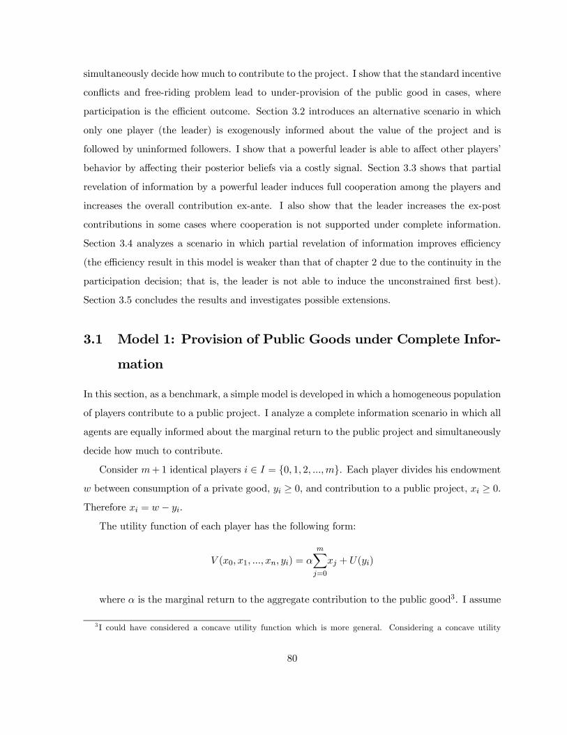
simultaneously decide how much to contribute to the project. I show that the standard incentive
conflicts and free-riding problem lead to under-provision of the public good in cases, where
participation is the efficient outcome. Section 3.2 introduces an alternative scenario in which
only one player (the leader) is exogenously informed about the value of the project and is
followed by uninformed followers. I show that a powerful leader is able to affect other players’
behavior by affecting their posterior beliefs via a costly signal. Section 3.3 shows that partial
revelation of information by a powerful leader induces full cooperation among the players and
increases the overall contribution ex-ante. I also show that the leader increases the ex-post
contributions in some cases where cooperation is not supported under complete information.
Section 3.4 analyzes a scenario in which partial revelation of information improves efficiency
(the efficiency result in this model is weaker than that of chapter 2 due to the continuity in the
participation decision; that is, the leader is not able to induce the unconstrained first best).
Section 3.5 concludes the results and investigates possible extensions.
3.1 Model 1: Provision of Public Goods under Complete Infor-
mation
In this section, as a benchmark, a simple model is developed in which a homogeneous population
of players contribute to a public project. I analyze a complete information scenario in which all
agents are equally informed about the marginal return to the public project and simultaneously
decide how much to contribute.
Consider m+1 identical players i ∈ I = {0, 1, 2, ...,m}. Each player divides his endowmentw between consumption of a private good, yi ≥ 0, and contribution to a public project, xi ≥ 0.Therefore xi = w − yi.
The utility function of each player has the following form:
V (x0, x1, ..., xn, yi) = αmXj=0
xj + U(yi)
where α is the marginal return to the aggregate contribution to the public good3. I assume
3I could have considered a concave utility function which is more general. Considering a concave utility
80

that α is distributed on the interval [0,α] with the density function f(α). I also assume that
U : <+ −→ < is a C3 function, which is strictly concave (U 00 < 0) and strictly monotone
increasing (U 0 > 0) over the interval [0, w]. Furthermore, I assume that Limy→0U
0(y) = +∞ and
Limy→∞ U 0(y) = 0 and players’ absolute risk aversion is non increasing, implying U 000 > 04.
Substituting for yi, players’ utility function can be written as:
bV (x0, x1, ..., xn) = αmXj=0
xj + U(w − xi)
I consider a simultaneous move game in which α is determined by the nature. All players
observe the realized value of α and simultaneously decide how much to contribute to the public
project.
A Nash equilibrium of the game is a vector of contributions³ eX(α)´ such that
eX(α) = Argmaxxi
αmXj=0
xj + U(w − xi) (2a)
Consider the maximization problem of a representative player. Each player decides to make
a zero or positive contribution. If the marginal return to the public project is small, such that
the player’s marginal utility of money exceeds the marginal return to the project, then he won’t
have any incentive to contribute to the project. For players to make a positive contribution, the
marginal return to the public project has to be at least as large as their marginal utility of money.
The following proposition represents this fact. Proposition 17 introduces players’ Contribution
Threshold under complete information: the smallest value of α above which players are willing
to make a positive contribution to the project. Most proofs including that of Proposition 17
are collected in the appendix.
Proposition 17 There exists a threshold eα such thatX(α) = 0 if α < eα
function, however, introduces more complexities but no new phenomenon of interest.4Player i’s absolute risk aversion is non increasing if −U
000U0+U002U02 ≤ 0. Since u0 > 0 by assumption, U 000 should
be positive for the inequality to be held.
81

X(α) = 1 if α > eαSee the appendix for the proof.
The threshold eα represents the smallest value of α above which players are willing to makea positive contribution. For α > eα, players’ optimal contribution level eX(α) is positive andresults from the following first order condition:
α =∂U
∂xi
This condition states that player i’s optimal contribution level must set his marginal utility
of money equal to the marginal return to the public project. Since U 00 < 0, Limy→0 U
0(y) = ∞and Lim
y→∞ U 0(y) = 0, for α > eα an interior solution exists and the above first order conditionis necessary and sufficient for the existence of a unique maximum. The following lemma shows
that once player i decides to participate to the public project, his contribution is a concave
function of α. This lemma is used in future proofs.
Lemma 18 For any α > eα player i’s optimal contribution eX(α) is a concave function of α.See the appendix for the proof.
For α < eα, the dominant strategy is not to contribute to the project. One motivation for mywork is the observation (shown below) that players may refuse to make a positive contribution
even when it is efficient to do so.
To see this define
∆W (α) = (m+ 1) [α(m+ 1)X(α) + U(w −X(α))− U(w)]
to be the welfare gain obtained by the group for the positive contribution X(α). If ∆W (α) > 0
for some α < eα, then the efficient outcome is to contribute to the public project. Positivecontribution, however, is not supported at the equilibrium by the implication of Lemma 1.
This illustrates the standard free-riding problem that leads to underprovision of public goods
under complete information.
82
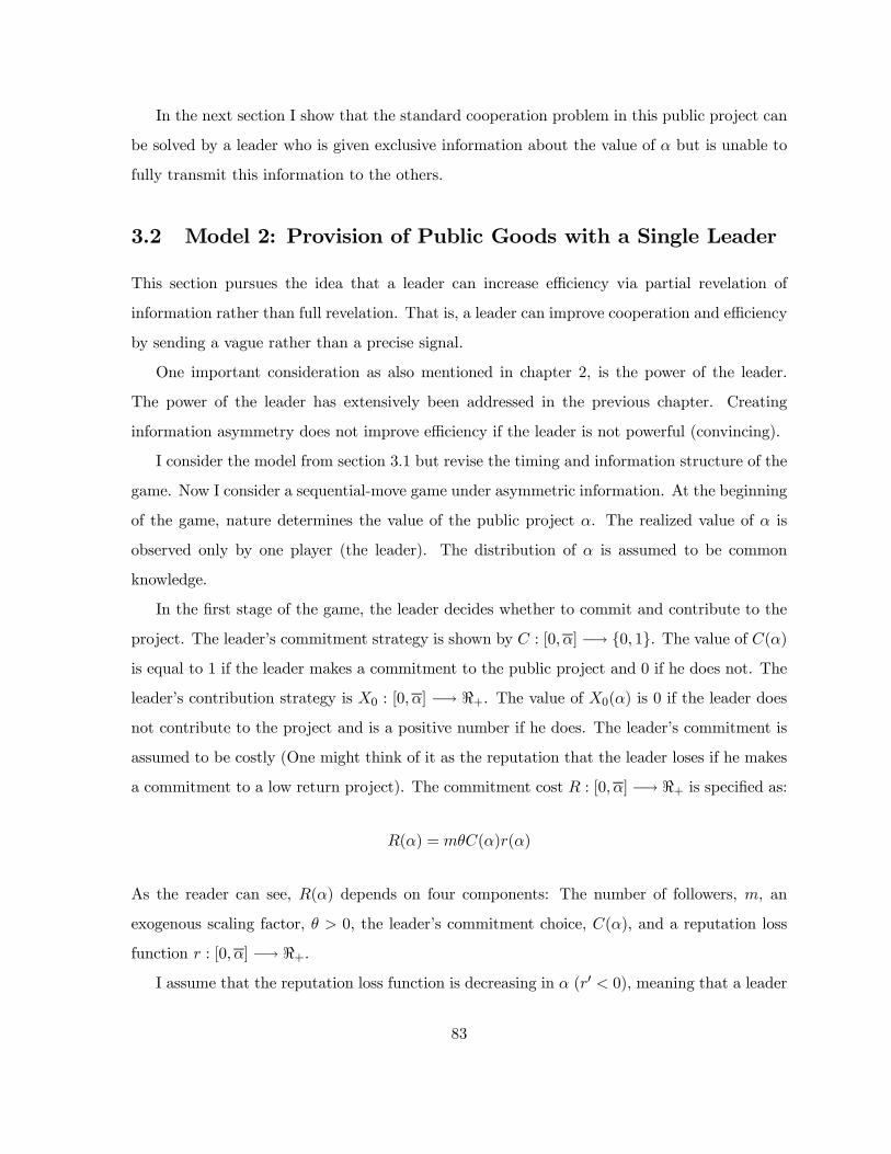
In the next section I show that the standard cooperation problem in this public project can
be solved by a leader who is given exclusive information about the value of α but is unable to
fully transmit this information to the others.
3.2 Model 2: Provision of Public Goods with a Single Leader
This section pursues the idea that a leader can increase efficiency via partial revelation of
information rather than full revelation. That is, a leader can improve cooperation and efficiency
by sending a vague rather than a precise signal.
One important consideration as also mentioned in chapter 2, is the power of the leader.
The power of the leader has extensively been addressed in the previous chapter. Creating
information asymmetry does not improve efficiency if the leader is not powerful (convincing).
I consider the model from section 3.1 but revise the timing and information structure of the
game. Now I consider a sequential-move game under asymmetric information. At the beginning
of the game, nature determines the value of the public project α. The realized value of α is
observed only by one player (the leader). The distribution of α is assumed to be common
knowledge.
In the first stage of the game, the leader decides whether to commit and contribute to the
project. The leader’s commitment strategy is shown by C : [0,α] −→ {0, 1}. The value of C(α)is equal to 1 if the leader makes a commitment to the public project and 0 if he does not. The
leader’s contribution strategy is X0 : [0,α] −→ <+. The value of X0(α) is 0 if the leader doesnot contribute to the project and is a positive number if he does. The leader’s commitment is
assumed to be costly (One might think of it as the reputation that the leader loses if he makes
a commitment to a low return project). The commitment cost R : [0,α] −→ <+ is specified as:
R(α) = mθC(α)r(α)
As the reader can see, R(α) depends on four components: The number of followers, m, an
exogenous scaling factor, θ > 0, the leader’s commitment choice, C(α), and a reputation loss
function r : [0,α] −→ <+.I assume that the reputation loss function is decreasing in α (r0 < 0), meaning that a leader
83
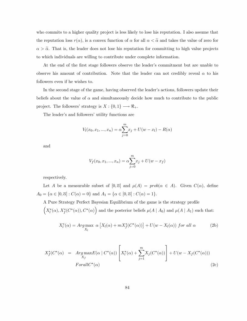
who commits to a higher quality project is less likely to lose his reputation. I also assume that
the reputation loss r(α), is a convex function of α for all α < eα and takes the value of zero forα > eα. That is, the leader does not lose his reputation for committing to high value projectsto which individuals are willing to contribute under complete information.
At the end of the first stage followers observe the leader’s commitment but are unable to
observe his amount of contribution. Note that the leader can not credibly reveal α to his
followers even if he wishes to.
In the second stage of the game, having observed the leader’s actions, followers update their
beliefs about the value of α and simultaneously decide how much to contribute to the public
project. The followers’ strategy is X : {0, 1} −→ <+.The leader’s and followers’ utility functions are
Vl(x0, x1, ..., xn) = αmXj=0
xj + U(w − xl)−R(α)
and
Vf (x0, x1, ..., xn) = αmXj=0
xj + U(w − xf )
respectively.
Let A be a measurable subset of [0,α] and µ(A) = prob(α ∈ A). Given C(α), define
A0 = {α ∈ [0,α] : C(α) = 0} and A1 = {α ∈ [0,α] : C(α) = 1}.A Pure Strategy Perfect Bayesian Equilibrium of the game is the strategy profile³X∗l (α),X
∗f (C
∗(α)), C∗(α)´and the posterior beliefs µ(A | A0) and µ(A | A1) such that:
X∗l (α) = ArgmaxXl
α£Xl(α) +mX
∗f (C
∗(α))¤+ U(w −Xl(α)) for all α (2b)
X∗f (C∗(α) = Argmax
Xf
E(α | C∗(α))X∗l (α) + mX
j=1
Xj(C∗(α))
+ U(w −Xf (C∗(α)))ForallC∗(α) (2c)
84
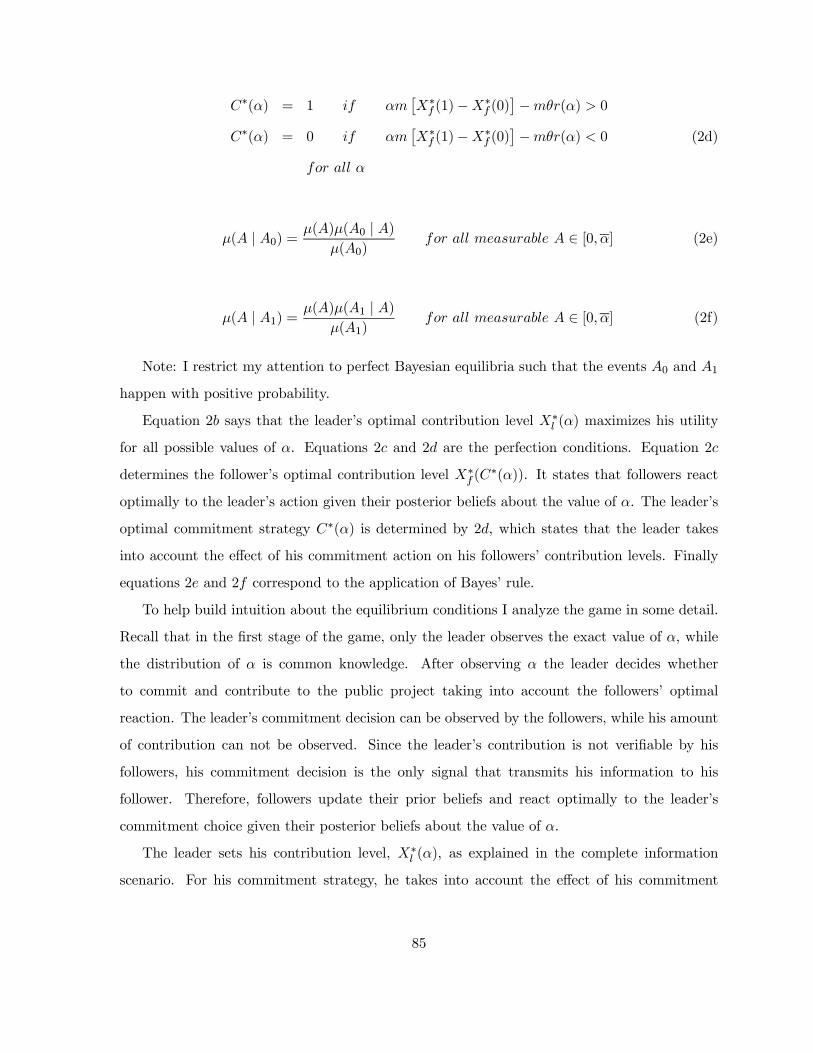
C∗(α) = 1 if αm£X∗f (1)−X∗f (0)
¤−mθr(α) > 0
C∗(α) = 0 if αm£X∗f (1)−X∗f (0)
¤−mθr(α) < 0 (2d)
for all α
µ(A | A0) = µ(A)µ(A0 | A)µ(A0)
for all measurable A ∈ [0,α] (2e)
µ(A | A1) = µ(A)µ(A1 | A)µ(A1)
for all measurable A ∈ [0,α] (2f)
Note: I restrict my attention to perfect Bayesian equilibria such that the events A0 and A1
happen with positive probability.
Equation 2b says that the leader’s optimal contribution level X∗l (α) maximizes his utility
for all possible values of α. Equations 2c and 2d are the perfection conditions. Equation 2c
determines the follower’s optimal contribution level X∗f (C∗(α)). It states that followers react
optimally to the leader’s action given their posterior beliefs about the value of α. The leader’s
optimal commitment strategy C∗(α) is determined by 2d, which states that the leader takes
into account the effect of his commitment action on his followers’ contribution levels. Finally
equations 2e and 2f correspond to the application of Bayes’ rule.
To help build intuition about the equilibrium conditions I analyze the game in some detail.
Recall that in the first stage of the game, only the leader observes the exact value of α, while
the distribution of α is common knowledge. After observing α the leader decides whether
to commit and contribute to the public project taking into account the followers’ optimal
reaction. The leader’s commitment decision can be observed by the followers, while his amount
of contribution can not be observed. Since the leader’s contribution is not verifiable by his
followers, his commitment decision is the only signal that transmits his information to his
follower. Therefore, followers update their prior beliefs and react optimally to the leader’s
commitment choice given their posterior beliefs about the value of α.
The leader sets his contribution level, X∗l (α), as explained in the complete information
scenario. For his commitment strategy, he takes into account the effect of his commitment
85
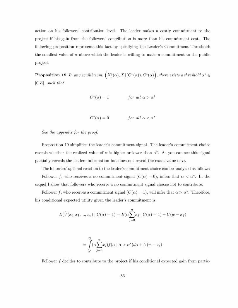
action on his followers’ contribution level. The leader makes a costly commitment to the
project if his gain from the followers’ contribution is more than his commitment cost. The
following proposition represents this fact by specifying the Leader’s Commitment Threshold:
the smallest value of α above which the leader is willing to make a commitment to the public
project.
Proposition 19 In any equilibrium,³X∗l (α),X
∗f (C
∗(α)), C∗(α)´, there exists a threshold α∗ ∈
[0,α], such that
C∗(α) = 1 for all α > α∗
C∗(α) = 0 for all α < α∗
See the appendix for the proof.
Proposition 19 simplifies the leader’s commitment signal. The leader’s commitment choice
reveals whether the realized value of α is higher or lower than α∗. As you can see this signal
partially reveals the leaders information but does not reveal the exact value of α.
The followers’ optimal reaction to the leader’s commitment choice can be analyzed as follows:
Follower f , who receives a no commitment signal (C(α) = 0), infers that α < α∗. In the
sequel I show that followers who receive a no commitment signal choose not to contribute.
Follower f , who receives a commitment signal (C(α) = 1), will infer that α > α∗. Therefore,
his conditional expected utility given the leader’s commitment is:
E(bV (x0, x1, ..., xn) | C(α) = 1) = E(α nXj=0
xj | C(α) = 1) + U(w − xf )
=
αZα∗
(αnXj=0
xj)f(α | α > α∗)dα+ U(w − xi)
Follower f decides to contribute to the project if his conditional expected gain from partic-
86

ipation is positive given the leader’s action, that is,
E(αnXj=0
xj | C(α)) + U(w − xi) > E(αnXj 6=ixj | C(α)) + U(w) for some xi > 0
For a follower who decides to make a positive contribution the first order condition implies
that E(α | C(α)) = ∂U
∂xi. Given the assumptions about the utility function once follower f
decides to contribute to the public project an interior solution exists and the above first order
condition is necessary and sufficient for the existence of a unique maximum X∗f (1).
As one can see from the above analysis, the contribution decision of an uninformed follower
depends on E(α | C(α)) rather than α itself. This enables a powerful leader to increase the
overall participation by manipulating his followers’ expectations via a vague signal. The next
section investigates this in detail.
3.3 Overall Contributions and the Single Leader
In this section I analyze three main issues. First, even if it is costless to inform everybody
about the quality of a project, it may improve cooperation to inform only one player. Second,
cooperation improves if the informed player (the leader) is unable to credibly reveal all of his
information. The third issue is about the leader’s power. The leader has the incentive to
exaggerate the value of the project, for he gets a large benefit from his followers’ participation.
Followers recognize such a leader and refuse to follow him. Appointing a single informed leader
will not improve efficiency unless we choose a player who is able to convince the rest. I will
specify the conditions sufficient to create a powerful leader.
This section is organized as the following. First, Proposition 21 shows that under incomplete
information followers base their contribution decision on E(α | C(α)) rather than α. Proposition22 addresses the power of leadership and specifies the condition under which the leader is
powerful enough to induce a following. I show that a powerful leader can increase expost
contributions to some low return but efficient projects. For cases where the expost result is
ambiguous, Theorem 23 states that a powerful leader increases the level of contribution ex-ante
(on average) by partial revelation of his private information.
87

Lemma 20 Recall that eα is the players’ complete information contribution threshold and g(α) =α eX(α) + U(w − eX(α)) − U(w) denotes player’s equilibrium utility gain from his contribution
to the public project under complete information. Then,
g(α) = 0 for all α < eα
g(α) > 0 for all α > eαSee the appendix for the proof.
Proposition 21 Consider the incomplete information scenario. Recall that follower f ’s ex-
pected utility function after observing a commitment decision is :
E(bV (x1, x2, ..., xn) | C(α)) = E(α nXj=1
xj | C(α)) + U(w − xf )
Because X∗f (C(α)) is optimal, E(α | C(α)) > eα implies X∗f (C(α)) > 0 and E(α | C(α)) < eαimplies X∗f (C(α)) = 0.
See the appendix for the proof.
Proposition 21 states that under incomplete information followers decide to make a positive
contribution if E(α | C(α)) is large enough to exceed eα. That is, they contribute if the leader’scommitment signal convinces them that the project yields a large personal payoff; large enough
to encourage participation even under complete information.
It can be shown that the leader’s commitment threshold α∗ is always below the complete in-
formation contribution threshold eα5. This means that, followers who observe a no commitmentsignal decide not to contribute to the project (X∗f (0) = 0).
Followers who observe a commitment signal choose to contribute if the leader’s commitment
is convincing them that α is high enough. A leader should not be willing to contribute for very
5By assumption r(α) = 0 for all α > eα. Therefore C(α) = 1 for all α > eα. This implies that α > α∗ for allα > eα. Therefore eα ≥ α∗
88

small values of α because he will not be convincing and therefore will not be followed by the
other players. The following proposition specifies the condition that a powerful leader should
satisfy.
Proposition 22 Consider the incomplete information scenario. Recall that α∗ is the leader’s
commitment threshold. There exists a threshold α∗c ∈ [0, eα], such that:E(α | C(α) = 1) > eα if α∗ > α∗c
E(α | C(α) = 1) < eα if α∗ < α∗c
See the appendix for the proof.
The threshold α∗c specified in Proposition 22, is called the Critical Threshold. A leader is
powerful if his commitment threshold exceeds α∗c . Lets assume that a powerful leader exists
and consider the possible scenarios that can occur from the ex-post point of view:
Case 1) α∗ < α ≤ eαCase 2) α < α∗ ≤ eαCase 3) α∗ ≤ eα < α
In Case 1, players refuse to contribute in the complete information scenario. Under incom-
plete information, however, the leader commits to the public good project (C(α) = 1) and
his commitment is followed by the others. Therefore, followers’ ex-post contribution under
incomplete information will exceed that of complete information.
In the second case, players refuse to participate in the public project under complete in-
formation. Under incomplete information the leader also refuses to commit to the project.
Therefore, nobody cooperates under either scenario.
In case three, everyone contributes in both complete and incomplete information scenarios,
but the size of the contributions may be different in each case. Whether followers contribute
more under complete or incomplete information depends on whether E(α | C(α)) is higher orlower than the true value of α.
In case three, there exists a range of α, (α ∈ (α∗, bα) , eα < bα < α), for which followers’
89

contributions under incomplete information exceeds those under complete information ex-post.
But ex-post contributions may be larger under complete information for higher values of α.
From the ex-ante point of view the incomplete information scenario seems less ambiguous.
Theorem 23 states that a powerful leader can increase follower’s expected contribution ex-ante.
Theorem 23 Given α∗ > α∗c , Eα
hX∗f (1)
i> E
α
h eX(α)iSee the appendix for the proof.
The above theorem states that followers who follow a powerful leader contribute more on
average.
A powerful leader can increase the average level of contribution above the complete informa-
tion scenario. An important issue, however, is how the leader’s exclusive access to information
affects the total surplus generated by the group. In the next section, I derive the efficiency
results for a special case with linear utility functions. In the future, I will develop the efficiency
analysis beyond the linear case presented in the next section.
3.4 Efficiency Improvements and the Single Leader
To analyze the welfare effects of the leader’s information advantage, I consider the following
scenario with linear utility functions.
Suppose that players’ utility functions are linear in the overall return to the public project
and consumption of the private good:
bV (x0, x1, ..., xn) = αnXj=1
xj +w − xi
As in the previous model, xi ≥ 0 is the amount of contribution and α is the marginal returnto the aggregate contribution to the public project.
In the complete information scenario, players’ optimal contribution level is the result of the
following first order condition:
∂ bV (x0, x1, ..., xn)∂xi
= α− 1 = 0
90

Therefore,
eX(α) = w, for α > 1
eX(α) = 0, for α < 1
eX(α) ∈ [0, w], for α = 1
That is under complete information, players are willing to contribute all their endowment
if α is greater than their complete information contribution threshold eα = 1 and they have noincentive to contribute if α is less than eα = 1.
In the incomplete information scenario, however, the story is different. In this example as
in the previous model, the leader moves first, deciding whether to commit and how much to
contribute to the project with only his commitment decision being observable by the followers.
As in the previous models, I assume that the leader’s commitment to the public project is costly
and the cost of commitment is R(α) = nθC(α)r(α), with r0 < 0 and r00 > 0. Followers extract
information from the leader’s commitment decision and decide how much to contribute to the
project.
Under such circumstances, there exists an equilibrium in which the leader commits to the
project and is followed by the others if the following conditions hold:
α > α∗ =θr(α∗)w
6 (i)
E(α | α ≥ α∗) > 1 (ii)
Condition (i) says that the realized value of α should be higher than the leader’s commitment
threshold α∗; that is it should be worthwhile for the leader to commit to the public project.
Condition (ii) states the condition under which the leader’s signal is powerful (convincing). This
condition states that followers’ expected value of α after observing the leader’s commitment,
should be greater than their complete information contribution threshold eα = 1, for it shouldbe worthwhile for them to contribute.
In the above equilibrium, for any α > 1, the followers’ contribution under incomplete in-
91
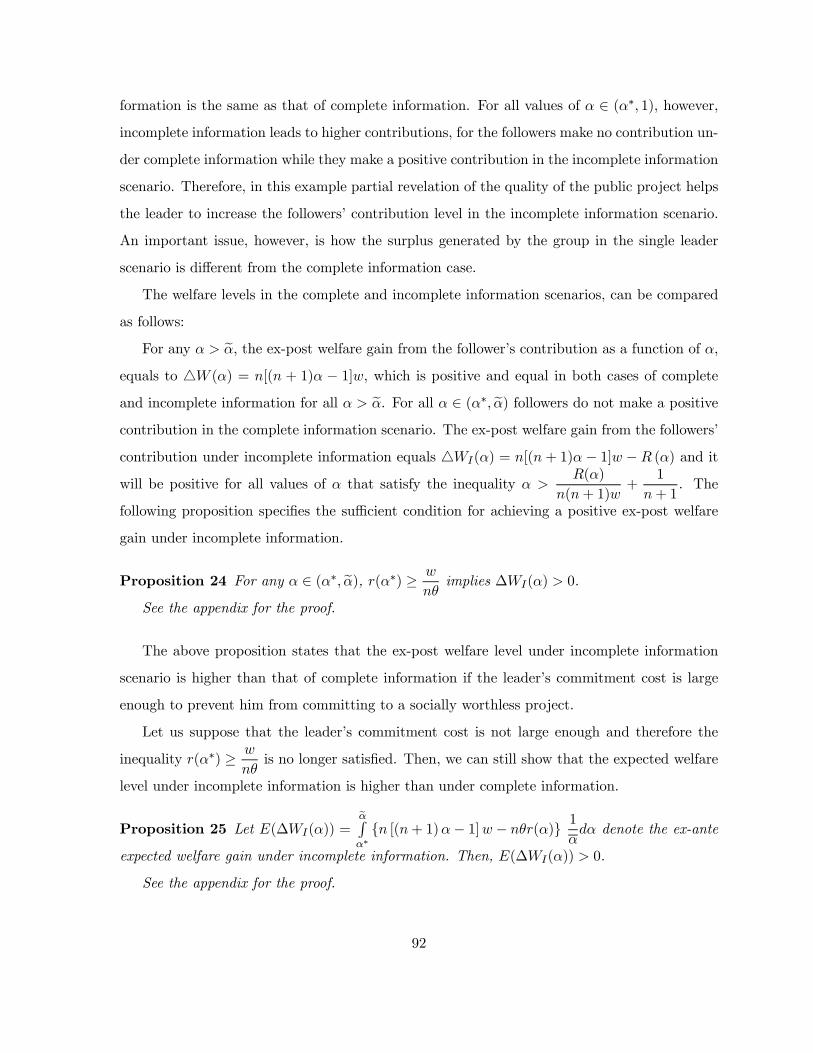
formation is the same as that of complete information. For all values of α ∈ (α∗, 1), however,incomplete information leads to higher contributions, for the followers make no contribution un-
der complete information while they make a positive contribution in the incomplete information
scenario. Therefore, in this example partial revelation of the quality of the public project helps
the leader to increase the followers’ contribution level in the incomplete information scenario.
An important issue, however, is how the surplus generated by the group in the single leader
scenario is different from the complete information case.
The welfare levels in the complete and incomplete information scenarios, can be compared
as follows:
For any α > eα, the ex-post welfare gain from the follower’s contribution as a function of α,
equals to 4W (α) = n[(n + 1)α − 1]w, which is positive and equal in both cases of completeand incomplete information for all α > eα. For all α ∈ (α∗, eα) followers do not make a positivecontribution in the complete information scenario. The ex-post welfare gain from the followers’
contribution under incomplete information equals 4WI(α) = n[(n+ 1)α − 1]w − R (α) and itwill be positive for all values of α that satisfy the inequality α >
R(α)
n(n+ 1)w+
1
n+ 1. The
following proposition specifies the sufficient condition for achieving a positive ex-post welfare
gain under incomplete information.
Proposition 24 For any α ∈ (α∗, eα), r(α∗) ≥ w
nθimplies ∆WI(α) > 0.
See the appendix for the proof.
The above proposition states that the ex-post welfare level under incomplete information
scenario is higher than that of complete information if the leader’s commitment cost is large
enough to prevent him from committing to a socially worthless project.
Let us suppose that the leader’s commitment cost is not large enough and therefore the
inequality r(α∗) ≥ w
nθis no longer satisfied. Then, we can still show that the expected welfare
level under incomplete information is higher than under complete information.
Proposition 25 Let E(∆WI(α)) =eαRα∗{n [(n+ 1)α− 1]w − nθr(α)} 1
αdα denote the ex-ante
expected welfare gain under incomplete information. Then, E(∆WI(α)) > 0.
See the appendix for the proof.
92

Proposition 25 states that the welfare level on average is higher under incomplete information
than that of complete information. This shows that the leader’s exclusive access to information
can improve efficiency ex-ante by partially transmitting his information to the others.
The following section concludes this chapter and discusses the further extensions.
3.5 Conclusion
A standard result of the theory of the public goods is that public goods are under-provided by
voluntary contributions.
I introduce leadership as an institutional solution to incentive conflicts and free-riding prob-
lems in public good games. By my definition, a leader is a person who has exclusive information
about the value of the public project.
I introduce a game theoretic model of public good provision under two different scenarios:
the complete information scenario and the incomplete information scenario.
In the single leader scenario, the leader is exogenously informed about the return to the
public project and is able to credibly transmit part of his information to the others by making
a costly commitment. Comparing these two cases, I draw the following conclusions:
I show that under incomplete information a powerful leader who has exclusive access to
the information can increase the overall contribution and the welfare level if he is unable to
transmit all of his information to the others.
I argue that under fairly general assumptions the leader can increase his followers’ ex-post
contributions. In cases where the ex-post result is ambiguous, I show that the ex-ante contri-
butions are larger in the presence of a powerful leader than those of complete information. In
other words, a powerful leader can increase the followers’ average contributions under incom-
plete information.
A leader can not induce a following unless he is able to convince his followers that he is
transmitting the correct information. I specify the condition under which the leader is powerful
enough to induce a following.
I also consider a scenario with linear utility functions and show that a powerful leader
can increase the ex-post social surplus if his commitment cost is large enough to prevent him
93

from committing to a socially worthless project. In cases where the ex-post welfare result is
ambiguous, I show that the ex-ante welfare in a single leader scenario is higher than that under
complete information, meaning that a powerful leader can increase the average welfare level.
In the future I seek to derive the welfare results for the more general utility function described
in the model.
3.6 Appendix
Proof of Proposition 17:
Let g(α) = α eX(α) + U(w − eX(α)) − U(w) denote the equilibrium utility gain from player
i’s contribution to the public project. Clearly g(α) > 0 implies eX(α) > 0.If eX(α) = 0 for all α ∈ [0,α], then eα = α.
Suppose eX(bα) > 0 for some bα ∈ [0,α]. Then g(bα) ≥ 0 and we have: g(α) ≥ α eX(bα)+U(w−eX(bα))− U(w) > g(bα) ≥ 0 for all α > bα. This implies that eX(α) > 0 for all α > bα.Summarizing: eX(bα) > 0 for some bα ∈ [0,α] implies that eX(α) > 0 for all α > bα. Pickeα = Inf nα : eX(α) > 0o.Proof of Lemma 18:
For any α > eα, player i’s optimization problem with respect to the private good yi, takes
the following form:
Maxyi
eV (yi) = αnXj=1
(w − yj) + U(yi)
The first order condition implies that:
U 0(yi) = α
Since U is strictly concave U 0 is invertible and:
£U 0¤−1
(α) = yi
94

Therefore, player i’s contribution as a function of α is the following:
eX(α) = w − £U 0¤−1 (α)Let [U 0]−1 (α) = g(α) and f(yi) = g−1(yi) = U 0(yi). According to our assumptions f 0(yi) is
well defined and non-zero. Therefore, Inverse Function Theorem implies that:
f 0(yi) =1
g0 [f(yi)]for all yi > 0
Taking the derivative from both sides of the above equality we have:
f 00(yi) =−f 0(yi).g00 [f(yi)][g0 [f(yi)]]2
for all yi > 0
or
U 000(yi) =−U 00(yi).g00 [f(yi)]
[g0 [f(yi)]]2for all yi > 0
Since U 000(yi) > 0 and U 00(yi) < 0 by assumption, then g00 [f(yi)] > 0 for all yi > 0, implying
that g(α) = [U 0]−1 (α) is convex in α. This implies that eX(α) is concave in α.
Proof of Proposition 19:
Let h(α) = αn (X∗(1)−X∗(0))−nθr(α) denote the leader’s utility gain from the followers’
contribution if he commits to the project. Clearly, h(α) > 0 implies C(α) = 1 and h(α) < 0
implies C(α) = 0.
If C(α) = 0 for all α ∈ [0,α], then α∗ = α.
Suppose C(bα) = 1 for some bα ∈ [0,α]. Then h(bα) ≥ 0, implying that (X∗(1)−X∗(0)) > 0.We also know by assumption that r0(α) < 0. Thus we can conclude that h0(α) > 0 for all
α > bα. This implies that h(α) > 0 for all α > bα. Therefore C(α) = 1 for all α > bα.Summarizing: C(bα) = 1 for some bα ∈ [0,α], implies C(α) = 1 for all α > bα. Pick
α∗ = Inf {α : C(α) = 1}.
Proof of Lemma 20:
95
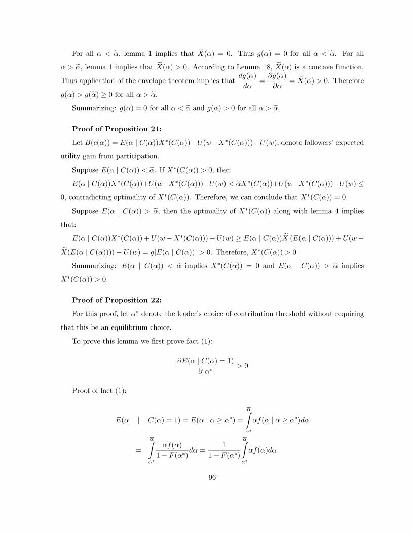
For all α < eα, lemma 1 implies that eX(α) = 0. Thus g(α) = 0 for all α < eα. For allα > eα, lemma 1 implies that eX(α) > 0. According to Lemma 18, eX(α) is a concave function.Thus application of the envelope theorem implies that
dg(α)
dα=
∂g(α)
∂α= eX(α) > 0. Therefore
g(α) > g(eα) ≥ 0 for all α > eα.Summarizing: g(α) = 0 for all α < eα and g(α) > 0 for all α > eα.Proof of Proposition 21:
Let B(c(α)) = E(α | C(α))X∗(C(α))+U(w−X∗(C(α)))−U(w), denote followers’ expectedutility gain from participation.
Suppose E(α | C(α)) < eα. If X∗(C(α)) > 0, thenE(α | C(α))X∗(C(α))+U(w−X∗(C(α)))−U(w) < eαX∗(C(α))+U(w−X∗(C(α)))−U(w) ≤
0, contradicting optimality of X∗(C(α)). Therefore, we can conclude that X∗(C(α)) = 0.
Suppose E(α | C(α)) > eα, then the optimality of X∗(C(α)) along with lemma 4 impliesthat:
E(α | C(α))X∗(C(α)) +U(w−X∗(C(α)))−U(w) ≥ E(α | C(α)) eX (E(α | C(α))) +U(w−eX(E(α | C(α))))− U(w) = g[E(α | C(α))] > 0. Therefore, X∗(C(α)) > 0.Summarizing: E(α | C(α)) < eα implies X∗(C(α)) = 0 and E(α | C(α)) > eα implies
X∗(C(α)) > 0.
Proof of Proposition 22:
For this proof, let α∗ denote the leader’s choice of contribution threshold without requiring
that this be an equilibrium choice.
To prove this lemma we first prove fact (1):
∂E(α | C(α) = 1)∂ α∗
> 0
Proof of fact (1):
E(α | C(α) = 1) = E(α | α ≥ α∗) =αZα∗
αf(α | α ≥ α∗)dα
=
αZα∗
αf(α)
1− F (α∗)dα =1
1− F (α∗)
αZα∗
αf(α)dα
96

Taking the derivative of E(α | α ≥ α∗) with respect to α∗ we have:
∂E(α | α ≥ α∗)∂ α∗
=f(α∗)
[1− F (α∗)]2αZα∗
αf(α)dα− α∗f(α∗)1− F (α∗)
=f(α∗)
1− F (α∗)
αZα∗
αf(α)
1− F (α∗)dα−α∗f(α∗)1− F (α∗)
>f(α∗)
1− F (α∗)
αZα∗
α∗f(α)1− F (α∗)dα−
α∗f(α∗)1− F (α∗)
=α∗f(α∗)1− F (α∗)
αZα∗
f(α)
1− F (α∗)dα− 1 = α∗f(α∗)
1− F (α∗) × 0 = 0
(Proof of fact 1 completed.)
Considering fact one,
If E(α | C(α) = 1) < eα for all α∗ ∈ [0, eα], then α∗c = eα.If E(α | C(α) = 1) > eα for all α∗ ∈ [0, eα], then α∗c = 0.
If E(α | C(α) = 1) = eα, let α∗c = α∗.
Proof of Theorem 23:
By definition eX(α) is the amount of player i’s contribution in the complete informationscenario that maximizes:
bV (x1, x2, ..., xn) = αnXj=1
xj + U(w − xi)
If α > eα (or if an interior solution exists), the first order condition for follower i impliesthat
α = U 0(w − eX(α)) (i)
By definition X∗(1) is the amount of follower i’s contribution under incomplete information
97
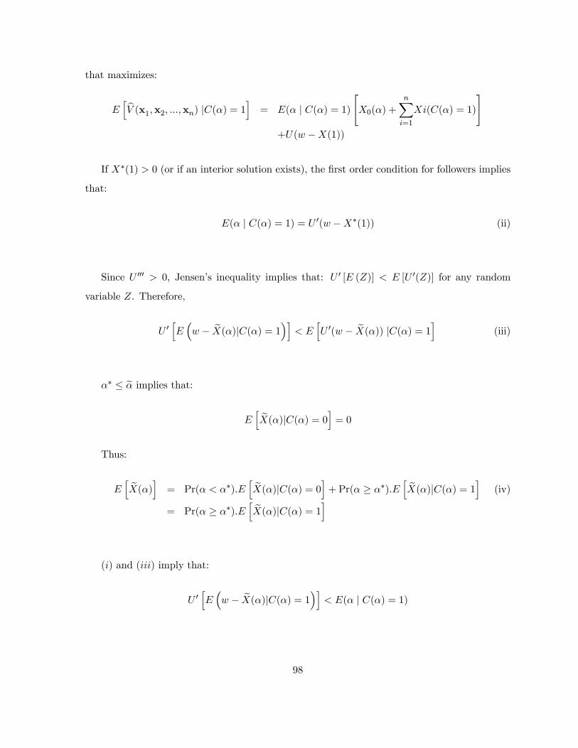
that maximizes:
EhbV (x1,x2, ...,xn) |C(α) = 1i = E(α | C(α) = 1)
"X0(α) +
nXi=1
Xi(C(α) = 1)
#+U(w −X(1))
If X∗(1) > 0 (or if an interior solution exists), the first order condition for followers implies
that:
E(α | C(α) = 1) = U 0(w −X∗(1)) (ii)
Since U 000 > 0, Jensen’s inequality implies that: U 0 [E (Z)] < E [U 0(Z)] for any random
variable Z. Therefore,
U 0hE³w − eX(α)|C(α) = 1´i < E hU 0(w − eX(α)) |C(α) = 1i (iii)
α∗ ≤ eα implies that:Eh eX(α)|C(α) = 0i = 0
Thus:
Eh eX(α)i = Pr(α < α∗).E
h eX(α)|C(α) = 0i+Pr(α ≥ α∗).Eh eX(α)|C(α) = 1i (iv)
= Pr(α ≥ α∗).Eh eX(α)|C(α) = 1i
(i) and (iii) imply that:
U 0hE³w − eX(α)|C(α) = 1´i < E(α | C(α) = 1)
98

Using (ii) we have:
U 0hE³w − eX(α)|C(α) = 1´i < U 0(w −X∗(1))
Because U 00 < 0 it follows that:
w −E³ eX(α)|C(α) = 1´ > w −X∗(1)
or
E³ eX(α)|C(α) = 1´ < X∗(1)
Thus,
Pr(α ≥ α∗).E³ eX(α)|C(α) = 1´ < Pr(α ≥ α∗).X∗(1)
Therefore from (iv) we have:
E [X∗(1)] > Eh eX(α)i
Proof of Proposition 24:
The inequality r(α∗) ≥ w
nθimplies that nθr(α∗) ≥ w. Adding θr(α∗) to both sides of the
inequality I have:
(n+ 1)θr(α∗)− w − θr(α∗) ≥ 0
If I multiply and divide the first term by w I get:
w(n+ 1)θr(α∗)w
− w − θr(α∗) ≥ 0
99

Since according to equation i, α∗ =θr(α∗)w
, I can rewrite the above inequality as:
(n+ 1)wα∗ − w − θr(α∗) ≥ 0
Multiplying both sides by n I get:
n [(n+ 1)α∗ − 1]w − nθr(α∗) ≥ 0
The above inequality simply shows that ∆WI(α) ≥ 0 at α = α∗. Since r0 < 0, ∆WI(α) is
an increasing function of α. Therefore ∆WI(α) ≥ 0 at α = α∗, implies that ∆WI(α) ≥ 0 forany α ∈ (α∗, eα).
Summarizing: r(α∗) ≥ w
nθimplies ∆WI(α) ≥ 0 for any α ∈ (α∗, eα).
Proof of Proposition 25:
Choose θ0 > 0 such that r(α∗) = θ0(eα− α∗) and define
A =
eαZα∗
©n [(n+ 1)α− 1]w − nθθ0(eα− α)
ª 1αdα
A =
eαZα∗
£n (n+ 1)αw − nw − nθθ0eα+ nθθ0α¤ 1
αdα
A =¡n2w + nw + nθθ0
¢ eαZα∗
α1
αdα− (nw + nθθ0eα) eαZ
α∗
1
αdα
A =¡n2w + nw + nθθ0
¢ ·α22α
¸eαα∗− (nw + nθθ0eα)·α
α
¸eαα∗
A =¡n2w + nw + nθθ0
¢ · w2 + 2wθθ0
2α(w2 + θ2θ02 + 2wθθ0)
¸−µnw
α
¶A =
n2w3 + 2n2w2θθ0 − nw3 − nw2θθ02α(w2 + θ2θ02 + 2wθθ0)
As it can be seen, A is positive for n > 0. By assumption r(α) is a convex function. This
implies that E(∆WI(α)) is a concave function of α. Therefore, E(∆WI(α)) > A > 0.
100

References1) Andreoni, James, Toward a Theory of Charitable Fund-Raising, Journal of Political
Economy, 1998, Vol. 106, no. 6.
2) Andreoni, James, Leadership Giving in Charitable Fund-Raising, Working Paper 2004.
3) Bergstrom, Theodore, Blume, Lawrance and Varian, Hall, On the Private Provision of
Public Goods, Journal of Public Economics, 1995, 29, 25-49.
4) Bryman, Alan, Leadership and Organizations, Book, Routledge & Kegan Paul, London,
Boston and Henley.
5) Cornes, R. and T. Sandler, Easy Riders, Joint Production and Public Goods, Economic
Journal, 1984, 94, 59-74.
6) Cornes, R. and T. Sandler, The Simple Analytics of Pure Public Good Provision, Eco-
nomica,1985,52, 103-116.
7) Castelnovo, Omri, Mayseless, Ofra, Popper, Micha, Transformational Leadership and
Attachment, Leadership Quarterly, Volume 11, Issue 2, Pages 267-289.
8) Dansereau, Fred, Yammarino, Francis, Leadership: The Multiple-level Approaches, Book,
1998, Jaipress Inc, Stanford, Connecticut, London, England.
9) Dansereau et al., Individualized Leadership: A New Multiple Level Approach, Leadership
Quarterly, Volume 6, Issue 3, Pages, 413-450.
10) Ehrlich, Sanford B., Meindle, James R., The Romance of Leadership and the evaluation
of Organizational Performance, The Academy of Management Journal, Volume 30, Issue 1,
March, 1987, Pages 91-109.
11) Ehrlich, Sanford B., Meindle, James R., Dukerich Janet M., The Romance of Leadership,
Administrative Science Quarterly, Volume 30, 1985, Pages 78-102.
12) Foss, Nicolai J., Leadership, Beliefs and Coordination: an Explorative Discussion, In-
dustrial and Corporate Changes, Volume 10, Number 2, 2001, Pages 357-388.
13) Hirshleifer, Jack, The Private and Social Value of Information and the Reward to
Inventive Activity, The American Economic Review, Vol. 61, No. 4, 561-574.
14) Hermalin, Benjamin E., Toward an Economic Theory of Leadership: Leading by Exam-
ple, American Economic Review, Vol 88, Issue 5, Dec. 1998, 1188-1206.
15) Hunt, James G., Ropo, Arja, Multi Level Leadership: Grounded Theory andMainstream
101
Theory Applied to the Case of General Motors, Leadership Quarterly, Volume 6, Issue 3, Pages
379-412.
16) Kim, Helen, Yukl, Gary, Relationships of Managerial Effectiveness and Advancement
to Self Reported and Subordinate Reported Leadership behaviors from the Multiple Linkage
Model, Leadership quarterly. Volume 6, Issue 3, Pages 361-377.
17) Kuhnert, Karl W., Lewis, Philip, Transactional and Transformational Leadership: A
Constructive/ Developmental Analysis, Academy of Management Review, 1987, Volume 12,
No. 4, Pages 648-657.
18) Kanungo, Rabindra N., Conger, Jay A., Toward a Behavioral Theory of Charismatic
Leadership in Organizational Settings, The academy of management review, Volume 12, Issue
4, October, 1987, Pages 637-647.
19) Lord, Robert, G., Mahr, Karen J., Leadership & Information Processing, Book, Rout-
ledge, London and New York.
20) Lord, Robert, G., Mahr, Karen J., Alternative Information Processing Models and their
Implications for Theory, Research and Practice, The Academy of Management Review, Volume
15, Issue 1, January, 1990, Pages 9-28.
21) Manz, Charles C., Self Leadership: Toward an Expanded Theory of Self-influence Pro-
cess in Organizations, The Academy of Management Review, Volume 11, Issue 3, July, 1986,
Pages 585-600.
22) Mueller, Bridget H., Lee Jaesub, Leader-Member Exchange and Organizational Com-
munication Satisfaction In Multiple Contexts, The journal of Business Communication, Volume
39, Issue 2, Pages 220-244.
23) Rhodes, Carl M., Wilson Rick K., Leaders, Followers, and the Situational Problem of
Trust, Working Paper.
24) Rhodes, Carl M., Wilson Rick K., Leadership and Credibility in N-person Coordination
Games, Journal of Conflict Resolution, Volume 41, number 6 December, 1997, Pages 767-791.
25) Romano, Richard and Huseyin Yildirim, Why Charities Announce Donations: A positive
Perspective, Manuscript, University of Florida, 1998.
26) Saloner, Garth, Rotemberg, Julio J., Leadership Style and Incentives, Management
Science, Volume 39, Issue 11, November 1993, Pages 1299-1318.
102
27) Sung, Yusen, Sequential versus Simultaneous Contribution Equilibria under Alternative
Public Good Specifications, Taiwan Economic Review,1998, 26: 4, 367-386.
28) Vecchio, Robert P., Leadership, Book, University of Notredame, Indiana.
29) Varian, Hal R., Sequential Provision of Public Goods, Journal of Public Economics,
1992, 53,165-86.
30) Vesterlund, Lise, The Informational Value of Sequential Fund-raising, Department of
Economics, Iowa State University, Working Paper, June 2000.
31) Vesterlund, Lise, Sefton, Martin, Potters, Jan, After You- Endogenous Sequencing in
Voluntary Contribution Games, Working Paper, April 2000.
32) Warr, P. G., The Private Provision of a Public Good Is Independent of the Distribution
of Incomes, Economic Letters, 1993, 13, 207-211.
103
Related Documents