An Early Warning Model for Predicting Credit Booms using Macroeconomic Aggregates

- Bogotá - Colombia - Bogotá - Colombia - Bogotá - Colombia - Bogotá - Colombia - Bogotá - Colombia - Bogotá - Colombia - Bogotá - Colombia - Bogotá - Colombia - Bogotá -

mtriansa

Cuadro de texto

An Early Warning Model for Predicting Credit Booms using Macroeconomic Aggregates Por:Alexander Guarín, Andrés González, Daphné Skandalis, Daniela Sánchez Núm. 723 2012

An Early Warning Model for Predicting Credit Booms using Macroeconomic

Aggregates∗

Alexander Guarí[email protected]

Andrés Gonzá[email protected]

Daphné [email protected]

Daniela Sá[email protected]

Banco de la República, Bogotá, Colombia.

Abstract

In this paper, we propose an alternative methodology to determine the existence of credit booms,which is a complex and crucial issue for policymakers. In particular, we exploit the Mendoza and Ter-rones (2008)’s idea that macroeconomic aggregates other than the credit growth rate contain valuableinformation to predict credit boom episodes. Our econometric method is used to estimate and predictthe probability of being in a credit boom. We run empirical exercises on quarterly data for six LatinAmerican countries between 1996 and 2011. In order to capture simultaneously model and parameteruncertainty, we implement the Bayesian model averaging method. As we employ panel data, the esti-mates may be used to predict booms of countries which are not considered in the estimation. Overall,our findings show that macroeconomic variables contain valuable information to predict credit booms.In fact, with our method the probability of detecting a credit boom is 80%, while the probability ofnot having false alarms is greater than 92%.

Keywords: Early Warning Indicator, Credit Booms, Business Cycles, Emerging Markets.

JEL Codes: E32, E37, E44, E51, C53

∗We would like to express our gratitude to Hernando Vargas and Sergio Ocampo for their valuable comments and suggestions andto Camila Fonseca for their assistance in the research work. The opinions expressed here are those of the authors and do not necessarilyrepresent neither those of the Banco de la República nor of its Board of Directors. As usual, all errors and omissions in this work areour responsibility.

1

2

1 Introduction

In general, a credit boom is defined as an excess of lending above its long-run trend. Credit booms tend tomake economies more volatile and vulnerable, and are often associated with increases in inflation, declinesin lending standards, instability in the banking sector and increases in the probability of a financial crisis(Reinhart and Kaminsky (2000), Gourinchas et al. (2001), Barajas et al. (2007), Dell’Ariccia et al. (2012)and Williams (2012)). Consequently, the identification of episodes of credit boom and their early predictionis a crucial problem for policymakers.

Nevertheless, the correct determination of these booms is a complex problem that is far from beingstraightforward in practice. The literature on credit booms has adopted several methodologies to identifyperiods of credit boom but none of them is fully satisfactory. Accordingly to one of these methods lendingboom periods are associated with high credit growth rates. Sachs et al. (1996), Borio and Lowe (2002),Kraft and Jankov (2005), Berkmen et al. (2009) and Frankel and Saravelos (2010) use the credit growthas an early warning indicator for predicting financial crises. However, Terrones (2004) points out thatperiods with high rates of credit growth can be the result of financial deepening, the economic cycle orthe catching up after recession periods. Hence, the dynamics of this rate alone is not a sufficient measureto define boom episodes.

Other strand of the literature characterizes lending booms as periods where the cyclical componentof credit exceeds a specific threshold. Moreover, it associates these boom episodes with the dynamics ofmacroeconomic aggregates (e.g. Gourinchas et al. (2001), Cottarelli et al. (2003), Kiss et al. (2006) andMendoza and Terrones (2008)). However, these works do not focus on the construction of quantitativeearly warning indicators of credit booms.

Our main contribution in this paper is the construction of an indicator that allows the identificationand the early prediction of credit boom episodes by exploiting the relationship between these latter andthe macroeconomic aggregates. Our indicator is based on two elements: the probability of being in acredit boom at time t+ h for h ≥ 0 conditioned on the set of data available up to time t, and second, onan estimated threshold value that establishes the probability at which the model defines the existence ofa credit boom.

The probabilities of credit boom are computed through a Bayesian average of many logistic regressionmodels applied to panel data. The Bayesian model averaging (BMA) methodology deals with parameterand model uncertainty. In our case, model uncertainty is related with the selection of the macroeconomicaggregates that should be included as explanatory variables in the logistic regression. The BMA runs alarge number of estimates on different combinations of covariates, and then, takes the weighted average ofall results. The weights are given by the model posterior probability.

The econometric analysis is applied on quarterly data of six Latin American countries between 1996and 2011. We run the BMA algorithm on two sets of covariates to test whether macroeconomic variablescontain additional information to the credit growth rate to explain credit boom episodes. The first setonly considers the macroeconomic aggregates as explanatory variables in the model while the second setadditionally includes the credit growth rate.

Our findings show that macroeconomic aggregates hold valuable information to identify the lendingboom episodes and to provide early warning signals about future booms. This is the case even if the creditgrowth rate is included as explanatory variable. The estimated probabilities of being in a credit boom attime t+ h with h ≥ 0 show an outstanding performance. For example, for our sample of Latin Americancountries, we estimate a threshold probability of 38%, which implies a probability of detecting a creditboom of 80.3% and a probability of not having false alarms greater than 92%.

We also carry out a cross-validation exercise across countries to check the reliability of our results.

3

Our findings indicate that the determinant factors of credit booms are similar across countries, and that,those factors can be captured with standard macroeconomic variables. These results also suggest that ouralgorithm may be used to predict lending booms of countries in the region that are not considered in theestimation and that may have short time series data.

Overall, this paper provides a valuable empirical tool to give a statistical response on the probabilityof being in a credit boom, or having a boom in the future. To the best of our knowledge, this is the firstpaper that performs the estimation and prediction of credit boom probabilities using macroeconomic data.In this sense both the methodology and the empirical results for our sample of Latin American countriesrepresent a new contribution to the burgeoning literature on credit booms.

The reminder of the paper is organized as follows. Section 2 presents the econometric methodology toestimate and predict the probability of being in a credit boom. This section also describes the estimationof the threshold probability. Section 3 goes into the details of the data set used in the empirical exercise.In Section 4 we perform the empirical exercises. Finally, Section 5 brings some conclusions.

2 Econometric Methodology

In order to estimate the probability of credit boom, we use the logistic regression model with panel dataand fixed effects

yi,t+h = αi + β′xit + εit i = 1, . . . , I t = 1, . . . , T (1)

where yi,t+h = 1 if there is a credit boom for country i at quarter t + h, h ≥ 0 and yi,t+h = 0 otherwise,β is a R × 1 parameter vector, εit is the error term and xit = (x1,it, . . . , xR,it) is a set of R covariates, αiwith i = 1, . . . , I are the fixed effects. These latter take into account the effect of omitted variables thatare specific to each country and affect the idiosyncratic credit boom probability.

Our aim is to estimate the probability of being in a credit boom at time t+ h with h ≥ 0 conditionedon the information up to time t through the following equation

p(yi,t+h = 1 | θ;xit) = F (αi + β′xit). (2)

where F is the cumulative logistic distribution function and θ = [α′ β′]′ with α = [α1, . . . , αI ]′ is the

parameter vector.In order to deal simultaneously with the model and parameter uncertainty, we apply the BMA method-

ology (see Raftery (1995) and Raftery et al. (1997)). We assume thatM = [M1, . . . ,MK ] is the set of allmodels, where Mk is the k-th model, which is defined as a subset of covariates of the set xit whose size isless or equal to R, θk is its associated parameter vector and D denotes the data set.

The BMA probability of being in a credit boom at time t+ h , h ≥ 0 is given by

pBMA (yi,t+h = 1 | D) =

K∑k=1

ˆp(yi,t+h = 1 | θk;D

)p(θk,Mk | D)dθk (3)

where p(θk,Mk | D) is the joint posterior probability. As can be seeing, the BMA probability in equation(3) is a weighted average of equation (2) where weights are given by p(θk,Mk | D). Since, the jointposterior probability is unknown, we approximate equation (3) using the reversible jump Markov chainMonte Carlo (RJMCMC) algorithm introduced by Green (1995) (see also Hoeting et al. (1999), Brookset al. (2003) and Green and Hastie (2009) for additional details).

Even though the probability pBMA (yi,t+h = 1 | D) is informative, it is interesting determine a value ofthis probability at which we have a clear warning of the existence of a credit boom. In other words, how

4

large does this probability need to be before calling for a credit boom? To answer this question, we definea threshold value, τ ∈ [0, 1], over which the methodology defines the warning. This estimation is carriedout through a variable yi,t+h (τ) defined as

yi,t+h (τ) =

{1 if p

(yi,t+h = 1 | θk;D

)≥ τ

0 otherwise.(4)

Note that for a given probability p(yi,t+h = 1 | θk;D

), the number of estimated credit booms depends

on the threshold τ . If this latter is very small, then we will have many warnings of credit boom which couldbe false alarms. On the contrary, if τ is very large, then we will have few warnings, and the probability ofhaving undetected booms would be large.

In order to define a threshold probability, we compute the value τ that

Min φ (τ) subject to γ (τ) ≤ γ (5)τε [0, 1]

where φ (τ) is the proportion of credit boom’s false alarms, γ (τ) is the proportion of undetected creditbooms and γ is the maximum value of γ admitted by the policymaker. The values of γ (τ) and φ (τ) areestimated as

γ (τ) =

∑Ii=1

∑Tt=1 1{(yi,t+h(τ)=0)∧(yi,t+h=1)}

T × I, (6)

φ (τ) =

∑Ii=1

∑Tt=1 1{(yi,t+h(τ)=1)∧(yi,t+h=0)}

T × I(7)

for h ≥ 0, where 1{·} is an indicator variable equal to 1 if condition {·} is satisfied, and 0 otherwise. Notethat the proportion {·} is calculated with respect to the total number of observations in the sample, andtherefore, γ (τ) and φ (τ) are different from the traditional Type I and II errors.

3 Data: Credit Booms and Macroeconomic Aggregates

We use quarterly data from Argentina, Brazil, Chile, Colombia, Mexico and Peru between the first quarter1996 and the fourth quarter 2011. Our set of covariates includes the macroeconomic aggregates highlightedby Mendoza and Terrones (2008) as relevant to determine credit booms: domestic economic activityvariables (Gross domestic product (GDP), investment, private consumption and government spending),international trade variables (terms of trade (ToT), real exchange rate (RER), current account), andfinancial system variables (asset prices and net capital flows). In specific exercises, we additionally includethe quarterly growth rate of the per-capita real credit. We include lagged values of the explanatoryvariables to capture the build up process of credit booms.

Data come from the International Monetary Found (IMF) and Central Banks websites1. The covariates:GDP, investment, private consumption, government spending and asset prices are seasonally adjusted andexpressed in real terms through the consumer price index (CPI). The RER corresponds to units of nationalcurrency for special drawing rights (SDR) of the IMF basket expressed in real terms with the CPI. TheToT are defined as the ratio between the prices of exportable and importable goods. We compute the

1Appendix A summarizes the set of covariates included in this research, the definition of each one and its specific source.

5

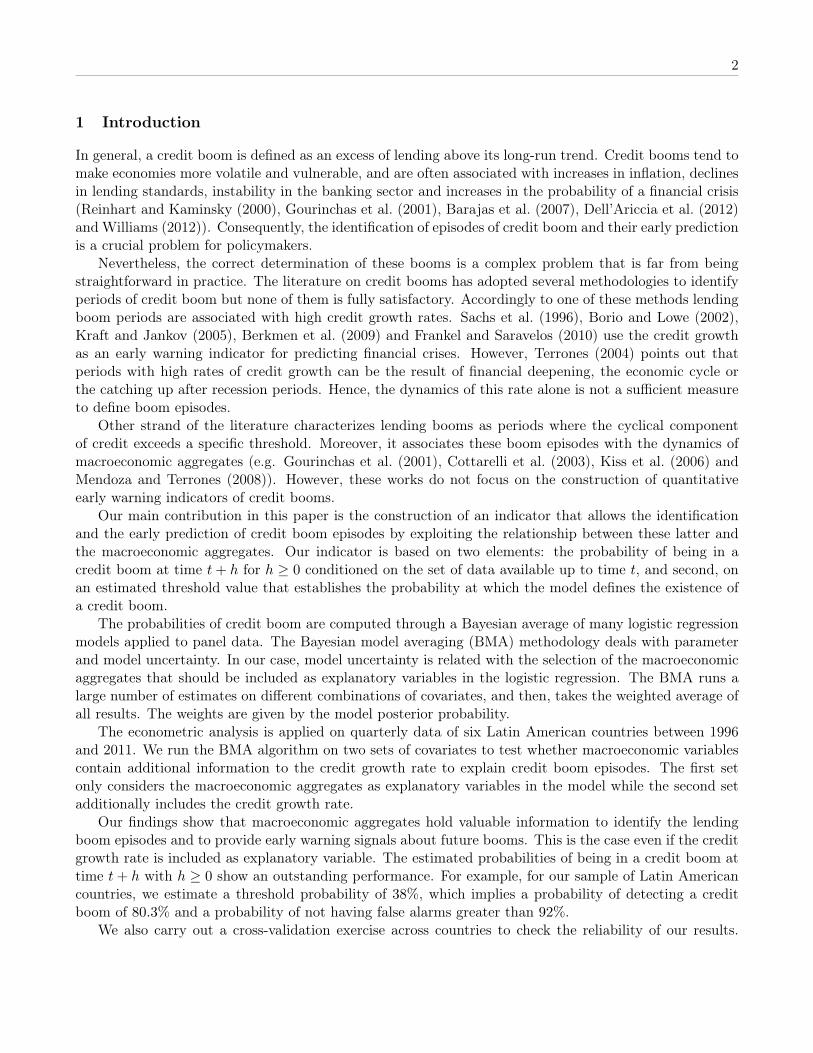
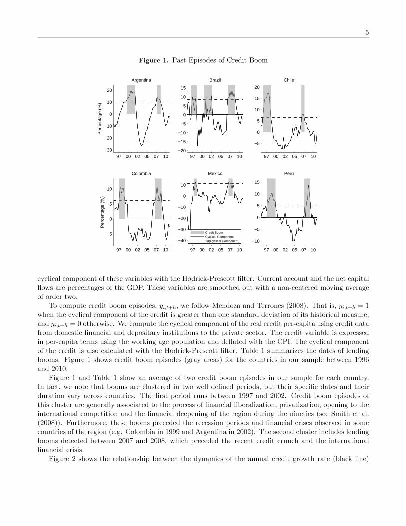
Figure 1. Past Episodes of Credit Boom

97 00 02 05 07 10−30

−20

−10

0

10

20

Per

cent

age

(%)

Argentina

97 00 02 05 07 10−20

−15

−10

−5

0

5

10

15

Brazil

97 00 02 05 07 10

−5

0

5

10

15

20

Chile

97 00 02 05 07 10

−5

0

5

10

Per

cent

age

(%)

Colombia

97 00 02 05 07 10

−40

−30

−20

−10

0

10

Mexico

97 00 02 05 07 10

−10

−5

0

5

10

15

Peru

Credit BoomCyclical Component1σ(Cyclical Component)

cyclical component of these variables with the Hodrick-Prescott filter. Current account and the net capitalflows are percentages of the GDP. These variables are smoothed out with a non-centered moving averageof order two.

To compute credit boom episodes, yi,t+h, we follow Mendoza and Terrones (2008). That is, yi,t+h = 1when the cyclical component of the credit is greater than one standard deviation of its historical measure,and yi,t+h = 0 otherwise. We compute the cyclical component of the real credit per-capita using credit datafrom domestic financial and depositary institutions to the private sector. The credit variable is expressedin per-capita terms using the working age population and deflated with the CPI. The cyclical componentof the credit is also calculated with the Hodrick-Prescott filter. Table 1 summarizes the dates of lendingbooms. Figure 1 shows credit boom episodes (gray areas) for the countries in our sample between 1996and 2010.

Figure 1 and Table 1 show an average of two credit boom episodes in our sample for each country.In fact, we note that booms are clustered in two well defined periods, but their specific dates and theirduration vary across countries. The first period runs between 1997 and 2002. Credit boom episodes ofthis cluster are generally associated to the process of financial liberalization, privatization, opening to theinternational competition and the financial deepening of the region during the nineties (see Smith et al.(2008)). Furthermore, these booms preceded the recession periods and financial crises observed in somecountries of the region (e.g. Colombia in 1999 and Argentina in 2002). The second cluster includes lendingbooms detected between 2007 and 2008, which preceded the recent credit crunch and the internationalfinancial crisis.

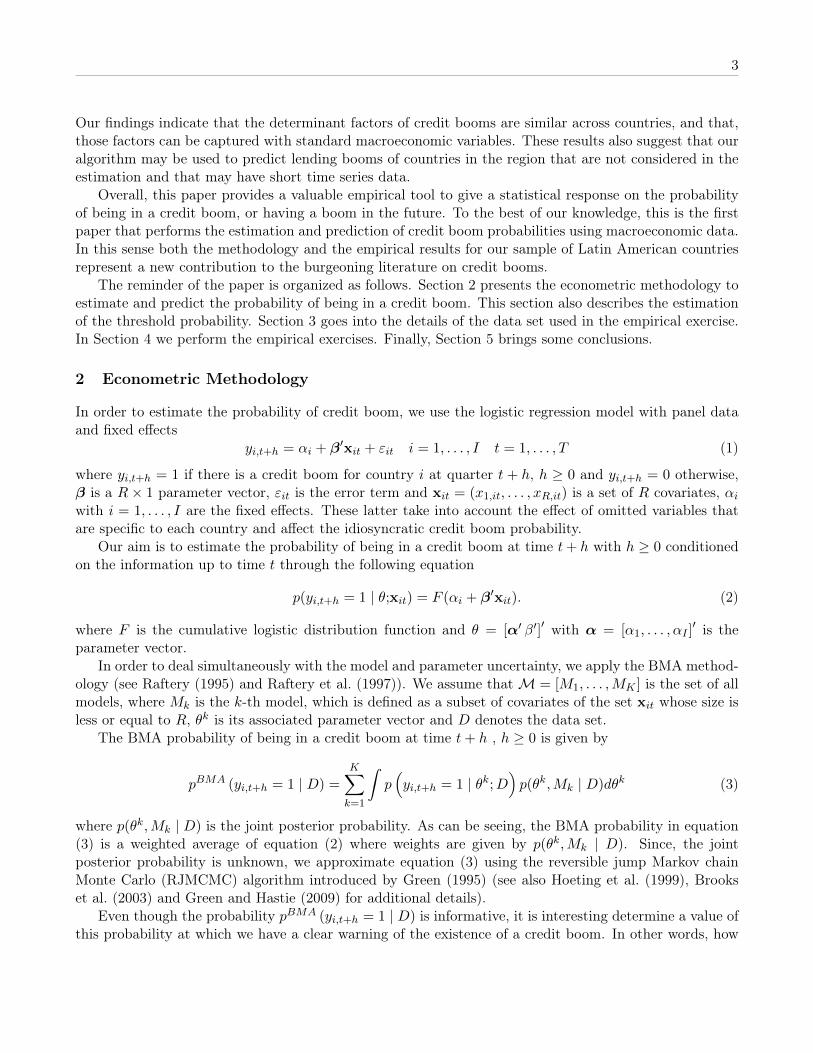
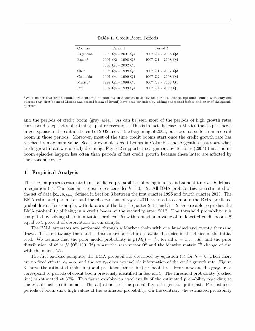
Figure 2 shows the relationship between the dynamics of the annual credit growth rate (black line)

6

Table 1. Credit Boom Periods

Country Period 1 Period 2

Argentina 1999 Q4 - 2001 Q4 2007 Q4 - 2008 Q3

Brazil* 1997 Q2 - 1998 Q3 2007 Q1 - 2008 Q4

2000 Q4 - 2002 Q3

Chile 1996 Q4 - 1998 Q3 2007 Q1 - 2007 Q3

Colombia 1997 Q4 - 1999 Q1 2007 Q2 - 2008 Q4

Mexico* 1998 Q1 - 1998 Q3 2007 Q2 - 2008 Q1

Peru 1997 Q4 - 1999 Q4 2007 Q4 - 2009 Q1

*We consider that credit booms are economic phenomena that last at least several periods. Hence, episodes defined with only onequarter (e.g. first boom of Mexico and second boom of Brazil) have been extended by adding one period before and after of the specificquarters.

and the periods of credit boom (gray area). As can be seen most of the periods of high growth ratescorrespond to episodes of catching up after recessions. This is in fact the case in Mexico that experience alarge expansion of credit at the end of 2002 and at the beginning of 2003, but does not suffer from a creditboom in those periods. Moreover, most of the time credit booms start once the credit growth rate hasreached its maximum value. See, for example, credit booms in Colombia and Argentina that start whencredit growth rate was already declining. Figure 2 supports the argument by Terrones (2004) that lendingboom episodes happen less often than periods of fast credit growth because these latter are affected bythe economic cycle.

4 Empirical Analysis

This section presents estimated and predicted probabilities of being in a credit boom at time t+h definedin equation (3). The econometric exercises consider h = 0, 1, 2. All BMA probabilities are estimated onthe set of data [xit, yi,t+h] defined in Section 3 between the first quarter 1996 and fourth quarter 2010. TheBMA estimated parameter and the observations of xit of 2011 are used to compute the BMA predictedprobabilities. For example, with data xit of the fourth quarter 2011 and h = 2, we are able to predict theBMA probability of being in a credit boom at the second quarter 2012. The threshold probability τ iscomputed by solving the minimization problem (5) with a maximum value of undetected credit booms γequal to 5 percent of observations in our sample.

The BMA estimates are performed through a Markov chain with one hundred and twenty thousanddraws. The first twenty thousand estimates are burned-up to avoid the noise in the choice of the initialseed. We assume that the prior model probability is p (Mk) = 1

K , for all k = 1, . . . ,K, and the priordistribution of θk is N

(0k, 100 · Ik

)where the zero vector 0k and the identity matrix Ik change of size

with the model Mk.The first exercise computes the BMA probabilities described by equation (3) for h = 0, when there

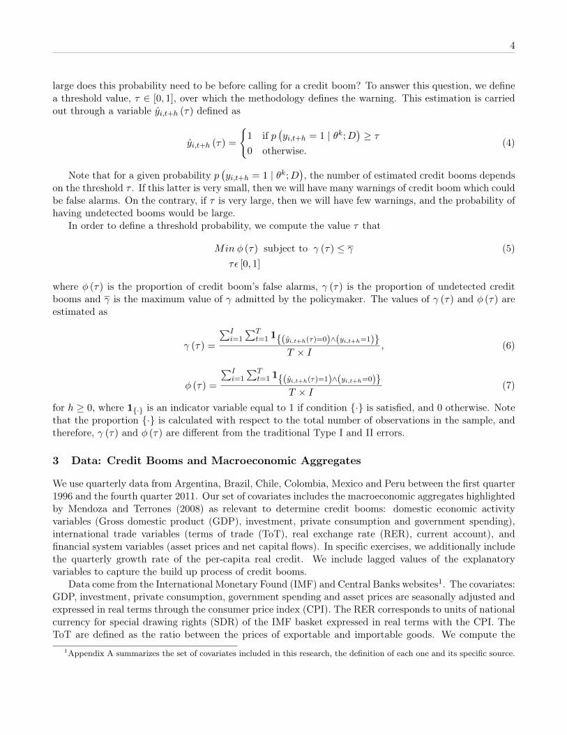
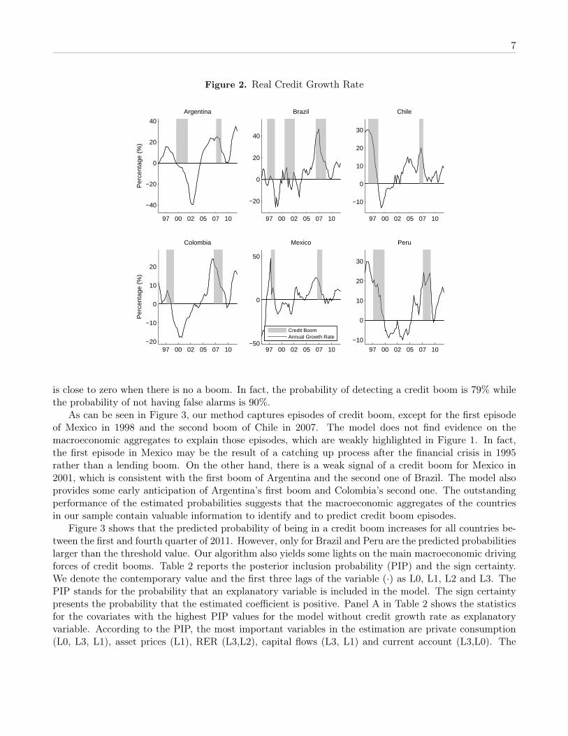
are no fixed effects, αi = α, and the set xit does not include information of the credit growth rate. Figure3 shows the estimated (thin line) and predicted (thick line) probabilities. From now on, the gray areascorrespond to periods of credit boom previously identified in Section 3. The threshold probability (dashedline) is estimated at 37%. This figure exhibits an excellent fit of the estimated probability regarding tothe established credit booms. The adjustment of the probability is in general quite fast. For instance,periods of boom show high values of the estimated probability. On the contrary, the estimated probability

7

Figure 2. Real Credit Growth Rate

97 00 02 05 07 10

−40

−20

0

20

40

Per

cent

age

(%)

Argentina

97 00 02 05 07 10

−20

0

20

40

Brazil

97 00 02 05 07 10

−10

0

10

20

30

Chile

97 00 02 05 07 10−20

−10

0

10

20

Per

cent

age

(%)

Colombia

97 00 02 05 07 10−50

0

50

Mexico

97 00 02 05 07 10

−10

0

10

20

30

Peru

Credit BoomAnnual Growth Rate

is close to zero when there is no a boom. In fact, the probability of detecting a credit boom is 79% whilethe probability of not having false alarms is 90%.

As can be seen in Figure 3, our method captures episodes of credit boom, except for the first episodeof Mexico in 1998 and the second boom of Chile in 2007. The model does not find evidence on themacroeconomic aggregates to explain those episodes, which are weakly highlighted in Figure 1. In fact,the first episode in Mexico may be the result of a catching up process after the financial crisis in 1995rather than a lending boom. On the other hand, there is a weak signal of a credit boom for Mexico in2001, which is consistent with the first boom of Argentina and the second one of Brazil. The model alsoprovides some early anticipation of Argentina’s first boom and Colombia’s second one. The outstandingperformance of the estimated probabilities suggests that the macroeconomic aggregates of the countriesin our sample contain valuable information to identify and to predict credit boom episodes.

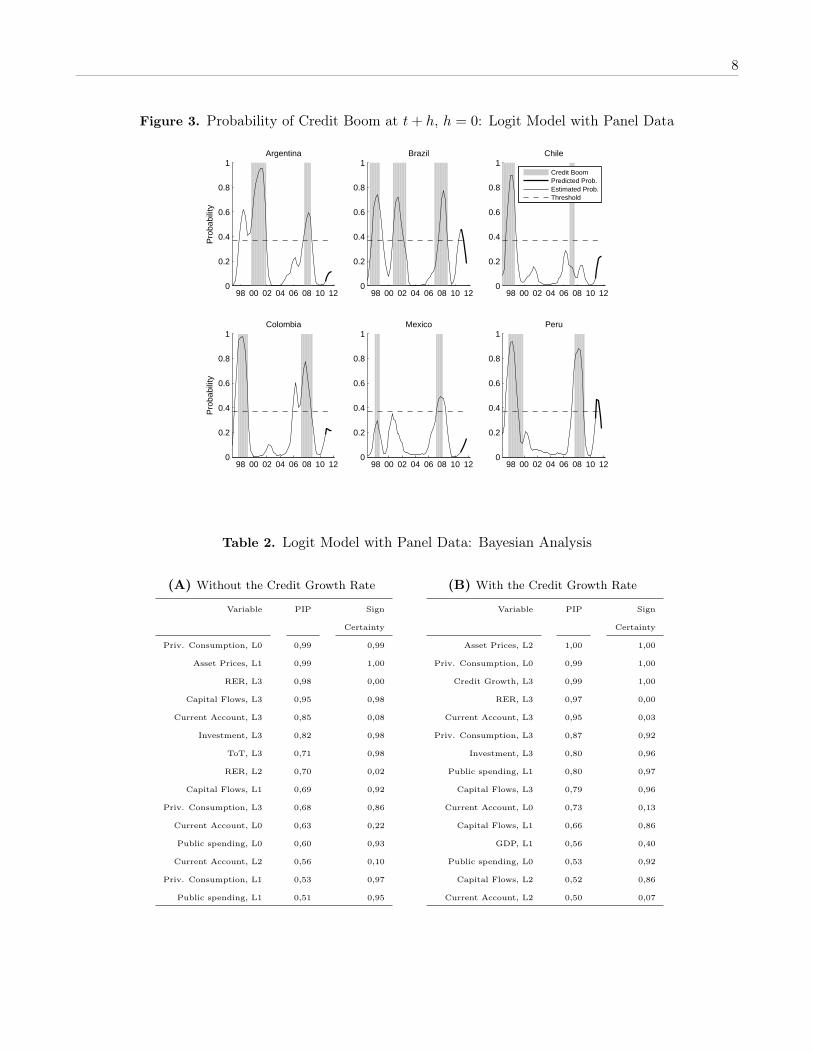
Figure 3 shows that the predicted probability of being in a credit boom increases for all countries be-tween the first and fourth quarter of 2011. However, only for Brazil and Peru are the predicted probabilitieslarger than the threshold value. Our algorithm also yields some lights on the main macroeconomic drivingforces of credit booms. Table 2 reports the posterior inclusion probability (PIP) and the sign certainty.We denote the contemporary value and the first three lags of the variable (·) as L0, L1, L2 and L3. ThePIP stands for the probability that an explanatory variable is included in the model. The sign certaintypresents the probability that the estimated coefficient is positive. Panel A in Table 2 shows the statisticsfor the covariates with the highest PIP values for the model without credit growth rate as explanatoryvariable. According to the PIP, the most important variables in the estimation are private consumption(L0, L3, L1), asset prices (L1), RER (L3,L2), capital flows (L3, L1) and current account (L3,L0). The

8

Figure 3. Probability of Credit Boom at t+ h, h = 0: Logit Model with Panel Data

98 00 02 04 06 08 10 120

0.2

0.4

0.6

0.8

1

Pro

babi

lity

Argentina

98 00 02 04 06 08 10 120

0.2

0.4

0.6

0.8

1Brazil

98 00 02 04 06 08 10 120

0.2

0.4

0.6

0.8

1Chile

Credit BoomPredicted Prob.Estimated Prob.Threshold

98 00 02 04 06 08 10 120

0.2

0.4

0.6

0.8

1

Pro

babi

lity

Colombia

98 00 02 04 06 08 10 120

0.2

0.4

0.6

0.8

1Mexico

98 00 02 04 06 08 10 120

0.2

0.4

0.6

0.8

1Peru

Table 2. Logit Model with Panel Data: Bayesian Analysis

(A) Without the Credit Growth Rate

Variable PIP Sign

Certainty

Priv. Consumption, L0 0,99 0,99

Asset Prices, L1 0,99 1,00

RER, L3 0,98 0,00

Capital Flows, L3 0,95 0,98

Current Account, L3 0,85 0,08

Investment, L3 0,82 0,98

ToT, L3 0,71 0,98

RER, L2 0,70 0,02




Public spending, L0 0,60 0,93




(B) With the Credit Growth Rate

Variable PIP Sign

Certainty



Credit Growth, L3 0,99 1,00

RER, L3 0,97 0,00








GDP, L1 0,56 0,40




9

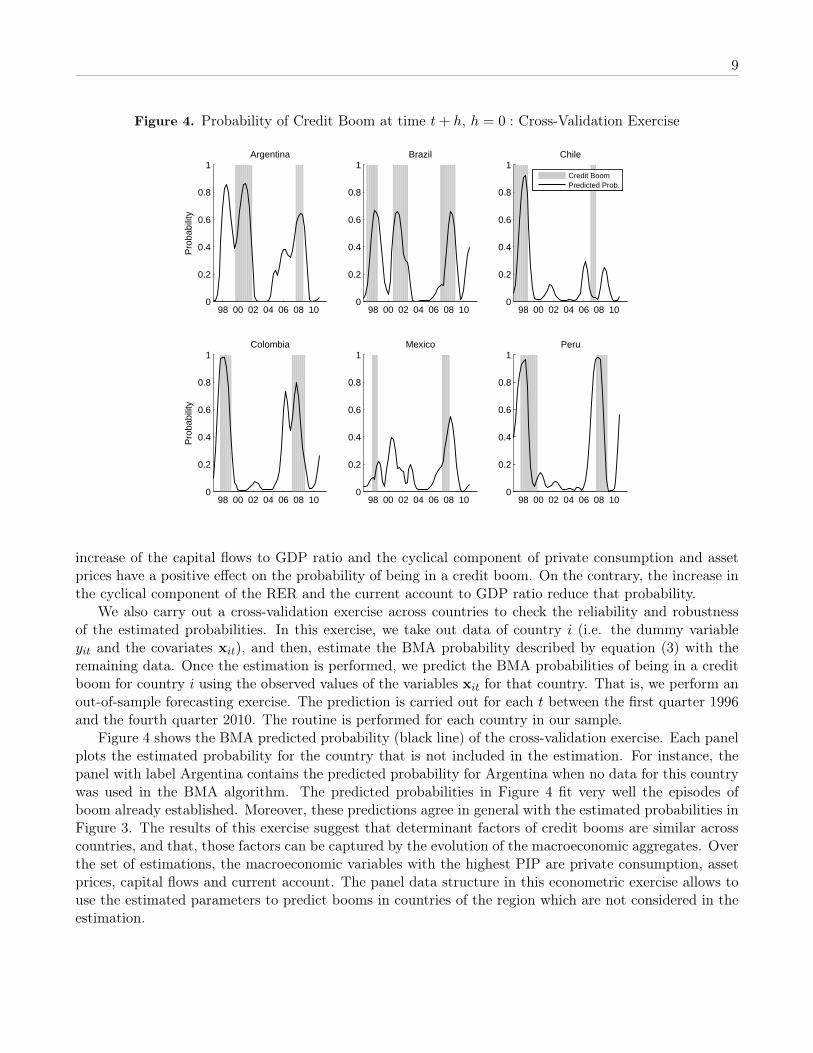
Figure 4. Probability of Credit Boom at time t+ h, h = 0 : Cross-Validation Exercise

98 00 02 04 06 08 100

0.2

0.4

0.6

0.8

1

Pro

babi

lity

Argentina

98 00 02 04 06 08 100

0.2

0.4

0.6

0.8

1Brazil

98 00 02 04 06 08 100

0.2

0.4

0.6

0.8

1Chile

Credit BoomPredicted Prob.

98 00 02 04 06 08 100

0.2

0.4

0.6

0.8

1

Pro

babi

lity

Colombia

98 00 02 04 06 08 100

0.2

0.4

0.6

0.8

1Mexico

98 00 02 04 06 08 100

0.2

0.4

0.6

0.8

1Peru

increase of the capital flows to GDP ratio and the cyclical component of private consumption and assetprices have a positive effect on the probability of being in a credit boom. On the contrary, the increase inthe cyclical component of the RER and the current account to GDP ratio reduce that probability.

We also carry out a cross-validation exercise across countries to check the reliability and robustnessof the estimated probabilities. In this exercise, we take out data of country i (i.e. the dummy variableyit and the covariates xit), and then, estimate the BMA probability described by equation (3) with theremaining data. Once the estimation is performed, we predict the BMA probabilities of being in a creditboom for country i using the observed values of the variables xit for that country. That is, we perform anout-of-sample forecasting exercise. The prediction is carried out for each t between the first quarter 1996and the fourth quarter 2010. The routine is performed for each country in our sample.

Figure 4 shows the BMA predicted probability (black line) of the cross-validation exercise. Each panelplots the estimated probability for the country that is not included in the estimation. For instance, thepanel with label Argentina contains the predicted probability for Argentina when no data for this countrywas used in the BMA algorithm. The predicted probabilities in Figure 4 fit very well the episodes ofboom already established. Moreover, these predictions agree in general with the estimated probabilities inFigure 3. The results of this exercise suggest that determinant factors of credit booms are similar acrosscountries, and that, those factors can be captured by the evolution of the macroeconomic aggregates. Overthe set of estimations, the macroeconomic variables with the highest PIP are private consumption, assetprices, capital flows and current account. The panel data structure in this econometric exercise allows touse the estimated parameters to predict booms in countries of the region which are not considered in theestimation.

10

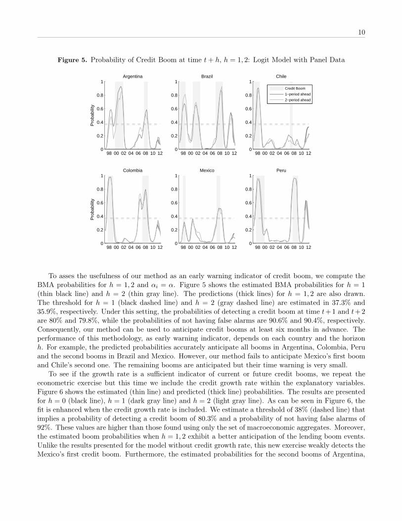
Figure 5. Probability of Credit Boom at time t+ h, h = 1, 2: Logit Model with Panel Data

98 00 02 04 06 08 10 120

0.2

0.4

0.6

0.8

1

Pro

babi

lity

Argentina

98 00 02 04 06 08 10 120

0.2

0.4

0.6

0.8

1Brazil

98 00 02 04 06 08 10 120

0.2

0.4

0.6

0.8

1Chile

98 00 02 04 06 08 10 120

0.2

0.4

0.6

0.8

1

Pro

babi

lity

Colombia

98 00 02 04 06 08 10 120

0.2

0.4

0.6

0.8

1Mexico

98 00 02 04 06 08 10 120

0.2

0.4

0.6

0.8

1Peru

Credit Boom

1−period ahead

2−period ahead

To asses the usefulness of our method as an early warning indicator of credit boom, we compute theBMA probabilities for h = 1, 2 and αi = α. Figure 5 shows the estimated BMA probabilities for h = 1(thin black line) and h = 2 (thin gray line). The predictions (thick lines) for h = 1, 2 are also drawn.The threshold for h = 1 (black dashed line) and h = 2 (gray dashed line) are estimated in 37.3% and35.9%, respectively. Under this setting, the probabilities of detecting a credit boom at time t+1 and t+2are 80% and 79.8%, while the probabilities of not having false alarms are 90.6% and 90.4%, respectively.Consequently, our method can be used to anticipate credit booms at least six months in advance. Theperformance of this methodology, as early warning indicator, depends on each country and the horizonh. For example, the predicted probabilities accurately anticipate all booms in Argentina, Colombia, Peruand the second booms in Brazil and Mexico. However, our method fails to anticipate Mexico’s first boomand Chile’s second one. The remaining booms are anticipated but their time warning is very small.

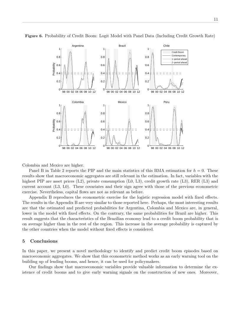
To see if the growth rate is a sufficient indicator of current or future credit booms, we repeat theeconometric exercise but this time we include the credit growth rate within the explanatory variables.Figure 6 shows the estimated (thin line) and predicted (thick line) probabilities. The results are presentedfor h = 0 (black line), h = 1 (dark gray line) and h = 2 (light gray line). As can be seen in Figure 6, thefit is enhanced when the credit growth rate is included. We estimate a threshold of 38% (dashed line) thatimplies a probability of detecting a credit boom of 80.3% and a probability of not having false alarms of92%. These values are higher than those found using only the set of macroeconomic aggregates. Moreover,the estimated boom probabilities when h = 1, 2 exhibit a better anticipation of the lending boom events.Unlike the results presented for the model without credit growth rate, this new exercise weakly detects theMexico’s first credit boom. Furthermore, the estimated probabilities for the second booms of Argentina,

11

Figure 6. Probability of Credit Boom: Logit Model with Panel Data (Including Credit Growth Rate)

98 00 02 04 06 08 10 120

0.2

0.4

0.6

0.8

1

Pro

babi

lity

Argentina

98 00 02 04 06 08 10 120

0.2

0.4

0.6

0.8

1Brazil

98 00 02 04 06 08 10 120

0.2

0.4

0.6

0.8

1Chile

98 00 02 04 06 08 10 120

0.2

0.4

0.6

0.8

1

Pro

babi

lity

Colombia

98 00 02 04 06 08 10 120

0.2

0.4

0.6

0.8

1Mexico

98 00 02 04 06 08 10 120

0.2

0.4

0.6

0.8

1Peru

Credit Boom

Contemporary

1−period ahead

2−period ahead

Colombia and Mexico are higher.Panel B in Table 2 reports the PIP and the main statistics of this BMA estimation for h = 0. These

results show that macroeconomic aggregates are still relevant in the estimation. In fact, variables with thehighest PIP are asset prices (L2), private consumption (L0, L3), credit growth rate (L3), RER (L3) andcurrent account (L3, L0). These covariates and their sign agree with those of the previous econometricexercise. Nevertheless, capital flows are not as relevant as before.

Appendix B reproduces the econometric exercise for the logistic regression model with fixed effects.The results in the Appendix B are very similar to those reported here. Perhaps, the most interesting resultsare that the estimated and predicted probabilities for Argentina, Colombia and Mexico are, in general,lower in the model with fixed effects. On the contrary, the same probabilities for Brazil are higher. Thisresult suggests that the characteristics of the Brazilian economy lead to a credit boom probability that ison average higher than in the rest of the region. This increase in the average probability is captured bythe other countries when the model without fixed effects is considered.

5 Conclusions

In this paper, we present a novel methodology to identify and predict credit boom episodes based onmacroeconomic aggregates. We show that this econometric method works as an early warning tool on thebuilding up of lending booms, and hence, it can be used for policymakers.

Our findings show that macroeconomic variables provide valuable information to determine the ex-istence of credit booms and to give early warning signals on the construction of new ones. Moreover,

12

our results suggest that the determinant factors of these boom episodes across countries are similar, andtherefore, our estimates can be used to predict booms of countries that are not considered in our sample.Even if the credit growth rate is included as explanatory variable, the macroeconomic variables remainrelevant to estimate and predict lending boom episodes.

The results show that the estimated probabilities of credit boom achieve a very good fit of episodespreviously determined by Mendoza and Terrones (2008)’s methodology. Nevertheless, if the credit growthrate is added to the set of covariates, the fit is enhanced.

References

Barajas, A., G. Dell’Ariccia, and A. Levchenko: 2007, ‘Credit Booms: The Good, The Bad and The Ugly’.Working paper, IMF.

Berkmen, P., G. Gaston, R. Rennhack, and J. Walsh: 2009, ‘The Global Financial Crisis: ExplainingCross-Country Differences in The Output Impact’. Journal of International Money and Finance 31,42–59.

Borio, C. and P. Lowe: 2002, ‘Asset Prices, Financial and Monetary Stability: Exploring The Nexus’.Working paper, BIS.

Brooks, S., F. N., and K. R.: 2003, ‘Classical Model Selection Via Simulated Annealing’. Journal of TheRoyal Statistical Society 65(2), 503–520.

Cottarelli, C., I. Vladkova, and G. Dell’Ariccia: 2003, ‘Early Birds, Late Risers, and Sleeping Beauties:Bank Credit Growth to The Private Sector in Central and Eastern Europe and in The Balkans’. WorkingPaper 03/213, IMF.

Dell’Ariccia, G., D. Igan, and L. Laeven: 2012, ‘Credit Booms and Lending Standards: Evidence FromThe Subprime Mortgage Market’. Journal of Money, Credit and Banking 44, 367–384.

Frankel, J. and G. Saravelos: 2010, ‘Are Leading Indicators of Financial Crises Useful for AssessingCountry Vulnerability? Evidence From The 2008-09 Global Crisis’. Working Paper 16047, NBER.

Gourinchas, P., R. Valdes, and O. Landerretche: 2001, ‘Lending Booms: Latin America and The World’.Working paper, NBER.

Green, P.: 1995, ‘Reversible Jump Markov Chain Monte Carlo Computation and Bayesian Model Deter-mination’. Biometrika 82(4), 711–732.

Green, P. and D. Hastie: 2009, ‘Reversible Jump MCMC’. Working paper, University of Helsinky.

Hoeting, J., D. Madigan, A. Raftery, and C. Volinsky: 1999, ‘Bayesian Model Averaging: A Tutorial’.Statistical Science 14(4), 382–417.

Kiss, G., M. Nagy, and B. Vonnák: 2006, ‘Credit Growth in Central and Eastern Europe: Convergence orBoom?’. Working paper, The Central Bank of Hungary.

Kraft, E. and L. Jankov: 2005, ‘Does Speed Kill? Lending Booms and Their Consequences in Croatia’.Journal of Banking & Finance 29(1), 105–121.

13

Mendoza, E. and M. Terrones: 2008, ‘An Anatomy of Credit Booms: Evidence From Macro Aggregatesand Micro Data’. Working paper, NBER.

Raftery, A.: 1995, ‘Bayesian Model Selection in Social Research’. Sociological Methodology 25, 111–164.

Raftery, A., D. Madigan, and J. Hoeting: 1997, ‘Bayesian Model Averaging for Linear Regression Models’.Journal of The American Statistical Association 92(437), 179–191.

Reinhart, C. and G. Kaminsky: 2000, ‘The Twin Crises: The Causes of Banking and Balance of PaymentsProblems’. MPRA Paper 13842, University Library of Munich, Germany.

Sachs, J., A. Tornell, and A. Velasco: 1996, ‘Financial Crises in Emerging Markets: The Lessons from1995’. Working Paper 5576, NBER.

Smith, J., T. Juhn, and C. Humphrey: 2008, ‘Consumer and Small Business Credit: Building Blocks ofThe Middle Class’. In: J. Haar and J. Price (eds.): Can Latin America Compete? Confronting TheChallenges of Globalization. Palgrave Macmillan.

Terrones, M.: 2004, ‘Are Credit Booms in Emerging Markets A Concern?’. In: World Economic Outlook.IMF, pp. 147–166.

Williams, G.: 2012, ‘Beyond The Credit Boom’. Working paper, The Institute for Public Policy Research.

14

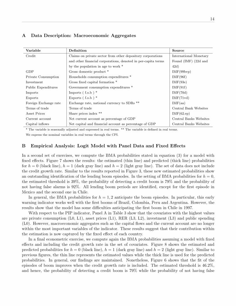
A Data Description: Macroeconomic Aggregates

Variable Definition SourceCredit Claims on private sector from other depository corporations

and other financial corporations, denoted in per-capita termsby the population in age to work *

International MonetaryFound (IMF) (22d and42d)

GDP Gross domestic product * IMF(99bvp)Private Consumption Households consumption expenditures * IMF(96f)Investment Gross fixed capital formation * IMF(93e)Public Expenditures Government consumption expenditures * IMF(91f)Imports Imports ( f.o.b ) * IMF(70d)Exports Exports ( f.o.b ) * IMF(71vd)Foreign Exchange rate Exchange rate, national currency to SDRs ** IMF(aa)Terms of trade Terms of trade Central Bank WebsitesAsset Prices Share prices index ** IMF(62.ep)Current account Net current account as percentage of GDP Central Banks WebsitesCapital inflows Net capital and financial account as percentage of GDP Central Banks Websites* The variable is seasonally adjusted and expressed in real terms. ** The variable is defined in real terms.

We express the nominal variables in real terms through the CPI.

B Empirical Analysis: Logit Model with Panel Data and Fixed Effects

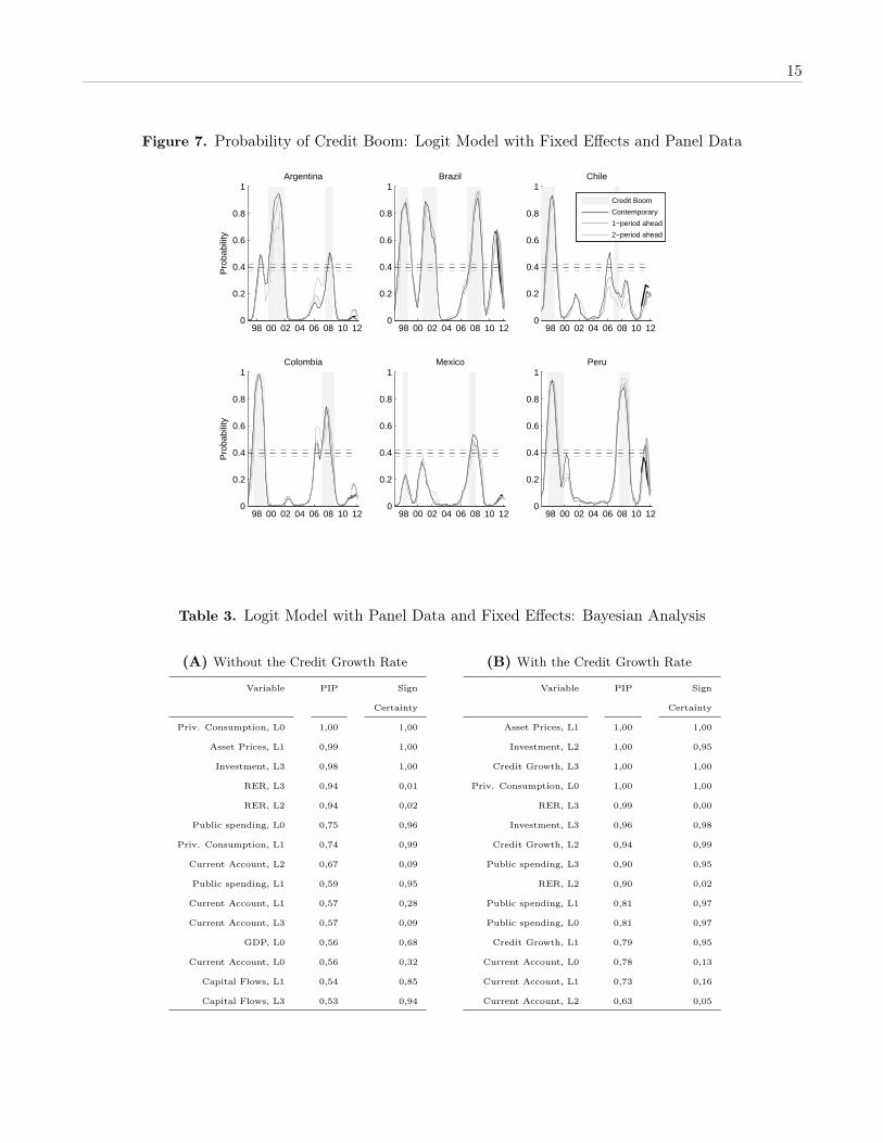
In a second set of exercises, we compute the BMA probabilities stated in equation (3) for a model withfixed effects. Figure 7 shows the results: the estimated (thin line) and predicted (thick line) probabilitiesfor h = 0 (black line), h = 1 (dark gray line) and h = 2 (light gray line). The set of data does not includethe credit growth rate. Similar to the results reported in Figure 3, these new estimated probabilities showan outstanding identification of the lending boom episodes. In the setting of BMA probabilities for h = 0,the estimated threshold is 39%, the probability of detecting a credit boom is 79% and the probability ofnot having false alarms is 92%. All lending boom periods are identified, except for the first episode inMexico and the second one in Chile.

In general, the BMA probabilities for h = 1, 2 anticipate the boom episodes. In particular, this earlywarning indicator works well with the first booms of Brazil, Colombia, Peru and Argentina. However, theresults show that the model has some difficulties anticipating the first boom in Chile in 1997.

With respect to the PIP indicator, Panel A in Table 3 show that the covariates with the highest valuesare private consumption (L0, L1), asset prices (L1), RER (L3, L2), investment (L3) and public spending(L0). However, macroeconomic aggregates such as the capital flows and the current account are no longerwithin the most important variables of the indicator. These results suggest that their contribution withinthe estimation is now captured by the fixed effect of each country.

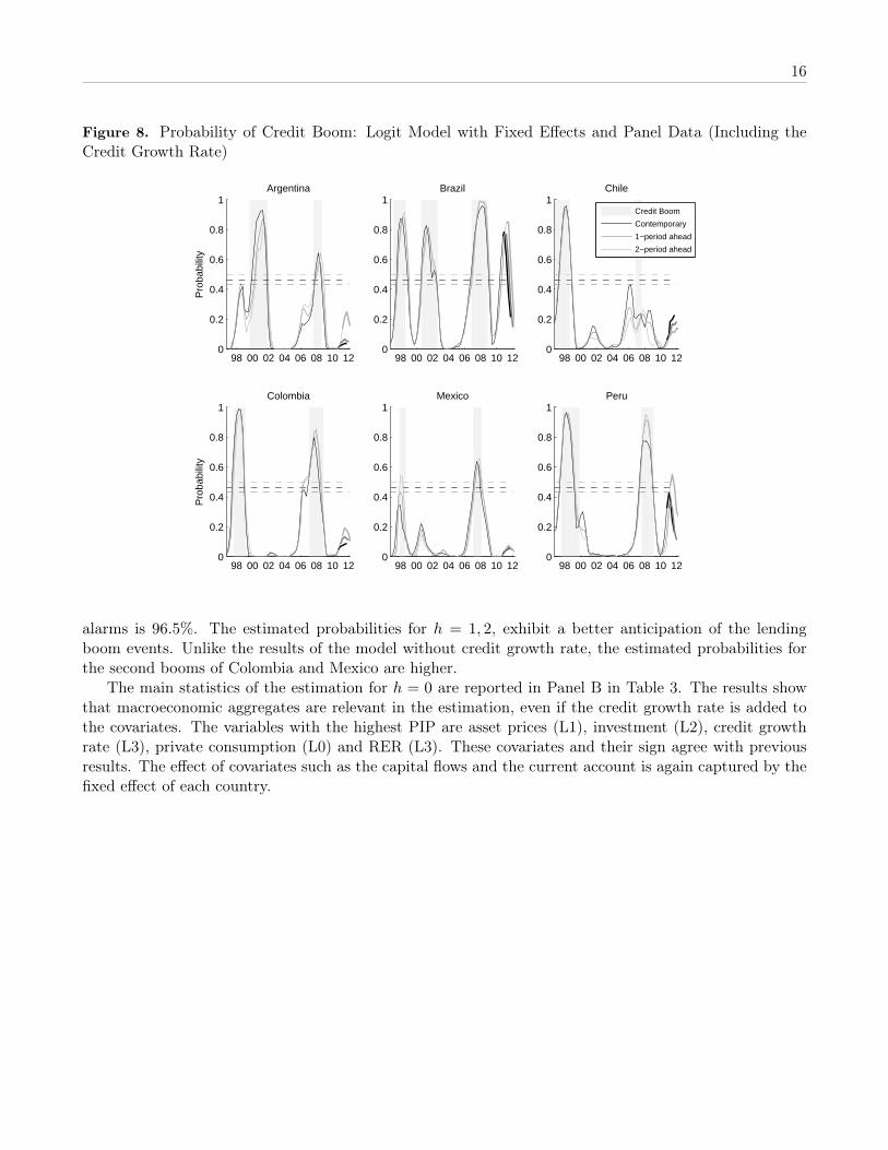
In a final econometric exercise, we compute again the BMA probabilities assuming a model with fixedeffects and including the credit growth rate in the set of covariates. Figure 8 shows the estimated andpredicted probabilities for h = 0 (black line), h = 1 (dark gray line) and h = 2 (light gray line). Similar toprevious figures, the thin line represents the estimated values while the thick line is used for the predictedprobabilities. In general, our findings are maintained. Nonetheless, Figure 6 shows that the fit of theepisodes of boom improves when the credit growth rate is included. The estimated threshold is 46.2%,and hence, the probability of detecting a credit boom is 79% while the probability of not having false

15

Figure 7. Probability of Credit Boom: Logit Model with Fixed Effects and Panel Data

98 00 02 04 06 08 10 120

0.2

0.4

0.6

0.8

1

Pro

babi

lity

Argentina

98 00 02 04 06 08 10 120

0.2

0.4

0.6

0.8

1Brazil

98 00 02 04 06 08 10 120

0.2

0.4

0.6

0.8

1Chile

98 00 02 04 06 08 10 120

0.2

0.4

0.6

0.8

1

Pro

babi

lity

Colombia

98 00 02 04 06 08 10 120

0.2

0.4

0.6

0.8

1Mexico

98 00 02 04 06 08 10 120

0.2

0.4

0.6

0.8

1Peru

Credit Boom

Contemporary

1−period ahead

2−period ahead

Table 3. Logit Model with Panel Data and Fixed Effects: Bayesian Analysis

(A) Without the Credit Growth Rate

Variable PIP Sign

Certainty




RER, L3 0,94 0,01

RER, L2 0,94 0,02







GDP, L0 0,56 0,68




(B) With the Credit Growth Rate

Variable PIP Sign

Certainty





RER, L3 0,99 0,00




RER, L2 0,90 0,02







16

Figure 8. Probability of Credit Boom: Logit Model with Fixed Effects and Panel Data (Including theCredit Growth Rate)

98 00 02 04 06 08 10 120

0.2

0.4

0.6

0.8

1P

roba

bilit

yArgentina

98 00 02 04 06 08 10 120

0.2

0.4

0.6

0.8

1Brazil

98 00 02 04 06 08 10 120

0.2

0.4

0.6

0.8

1Chile

98 00 02 04 06 08 10 120

0.2

0.4

0.6

0.8

1

Pro

babi

lity

Colombia

98 00 02 04 06 08 10 120

0.2

0.4

0.6

0.8

1Mexico

98 00 02 04 06 08 10 120

0.2

0.4

0.6

0.8

1Peru

Credit Boom

Contemporary

1−period ahead

2−period ahead

alarms is 96.5%. The estimated probabilities for h = 1, 2, exhibit a better anticipation of the lendingboom events. Unlike the results of the model without credit growth rate, the estimated probabilities forthe second booms of Colombia and Mexico are higher.

The main statistics of the estimation for h = 0 are reported in Panel B in Table 3. The results showthat macroeconomic aggregates are relevant in the estimation, even if the credit growth rate is added tothe covariates. The variables with the highest PIP are asset prices (L1), investment (L2), credit growthrate (L3), private consumption (L0) and RER (L3). These covariates and their sign agree with previousresults. The effect of covariates such as the capital flows and the current account is again captured by thefixed effect of each country.

An Early Warning Model for Predicting Credit Booms using Macroeconomic Aggregates

Documents