An AVO analysis project - Stanford · PDF file2 AVO group SEP–80 In this paper we present the Mobil AVO data set and describe our preliminary preprocess-ing work. We discuss model

Stanford Exploration Project, Report 80, May 15, 2001, pages 1–344

An AVO analysis project

C. Ecker, D. Lumley, S. Levin,T. Rekdal, A. Berlioux, R. Clapp, Y. Wang & J. Ji1

ABSTRACT

We present an AVO data set consisting of raw prestack seismic data, petrophysical infor-mation and well-logs. These data are the focus of an AVO workshop sponsored by Mobil.SEP’s AVO project goals include: true-amplitude preprocessing including multiple sup-pression, AVO analysis and impedance inversion, and developing lithologic/hydrocarbonindicators based on rock physics properties and seismic attributes. We discuss preliminaryresults in model building, synthetic seismogram generation and preprocessing, and brieflyoutline our planned research.

INTRODUCTION

Seismic reflections and their “amplitude variation with offset” (AVO) are related to subsur-face lithology and pore fluid content. In the last decade, seismic AVO analysis has becomeprominent in the direct detection of hydrocarbons, and in reducing exploration drilling risk.For example, Ostrander (1984) demonstrated the ability to distinguish “bright spots” causedby hydrocarbon gas from non-hydrocarbon related high-impedance contrast layers.

However, problems associated with AVO analysis may produce false indications of hydro-carbon presence. True-amplitude preprocessing, essential for subsequent amplitude analysis,may have difficulties associated with shot and amplitude balancing, multiple suppression, andcalibration of overburden amplitude corrections. Furthermore, the non-uniqueness and in-stability of some seismic inversion schemes often makes it difficult to correctly interpret thelithology and pore fluid content resulting from the AVO analysis. Hence, both true-amplitudepreprocessing and robust seismic inversion methods are of major concern for successful AVOanalyses.

This study introduces an AVO data set consisting of seismic, petrophysical and well-loginformation which was provided by Mobil as part of an AVO workshop. The prestack seismicdata are heavily contaminated with free-surface and water-bottom multiple reflections. Pri-mary goals of our project are to 1) measure the true AVO on the primary reflections by eithersuppressing or incorporating the interfering multiple reflection energy, 2) perform a subse-quent robust impedance inversion and correlate the results with the well-log and petrophysicaldata, and 3) devise AVO indicators relevant for these data using rock physical principles.

1email: not available

1

2 AVO group SEP–80

In this paper we present the Mobil AVO data set and describe our preliminary preprocess-ing work. We discuss model building and synthetic seismograms which we plan to use to testour true-amplitude preprocessing and multiple suppression methods. Finally, we give a briefoverview of our plans for AVO analysis and impedance inversions, and rock physics analysisof optimal AVO indicators.

MOBIL AVO DATA SET

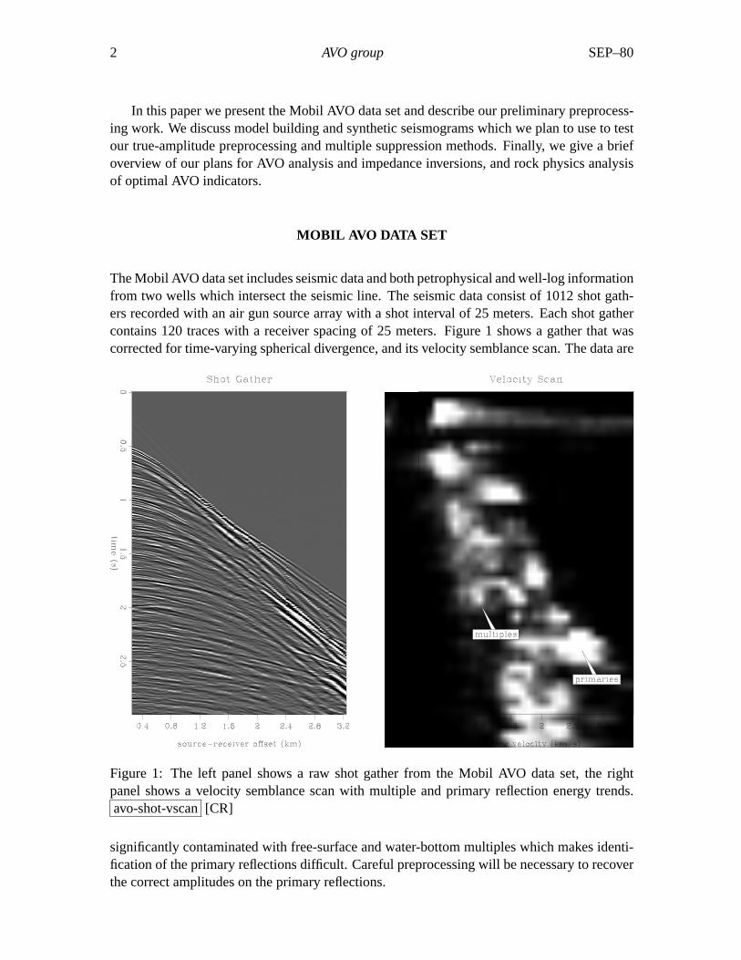
The Mobil AVO data set includes seismic data and both petrophysical and well-log informationfrom two wells which intersect the seismic line. The seismic data consist of 1012 shot gath-ers recorded with an air gun source array with a shot interval of 25 meters. Each shot gathercontains 120 traces with a receiver spacing of 25 meters. Figure 1 shows a gather that wascorrected for time-varying spherical divergence, and its velocity semblance scan. The data are

Figure 1: The left panel shows a raw shot gather from the Mobil AVO data set, the rightpanel shows a velocity semblance scan with multiple and primary reflection energy trends.avo-shot-vscan[CR]

significantly contaminated with free-surface and water-bottom multiples which makes identi-fication of the primary reflections difficult. Careful preprocessing will be necessary to recoverthe correct amplitudes on the primary reflections.

SEP–80 AVO project 3

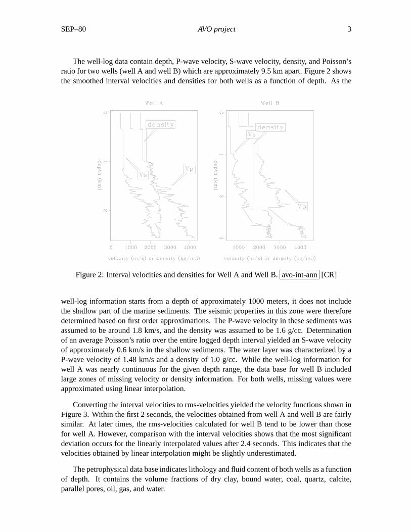
The well-log data contain depth, P-wave velocity, S-wave velocity, density, and Poisson’sratio for two wells (well A and well B) which are approximately 9.5 km apart. Figure 2 showsthe smoothed interval velocities and densities for both wells as a function of depth. As the

Figure 2: Interval velocities and densities for Well A and Well B.avo-int-ann[CR]

well-log information starts from a depth of approximately 1000 meters, it does not includethe shallow part of the marine sediments. The seismic properties in this zone were thereforedetermined based on first order approximations. The P-wave velocity in these sediments wasassumed to be around 1.8 km/s, and the density was assumed to be 1.6 g/cc. Determinationof an average Poisson’s ratio over the entire logged depth interval yielded an S-wave velocityof approximately 0.6 km/s in the shallow sediments. The water layer was characterized by aP-wave velocity of 1.48 km/s and a density of 1.0 g/cc. While the well-log information forwell A was nearly continuous for the given depth range, the data base for well B includedlarge zones of missing velocity or density information. For both wells, missing values wereapproximated using linear interpolation.

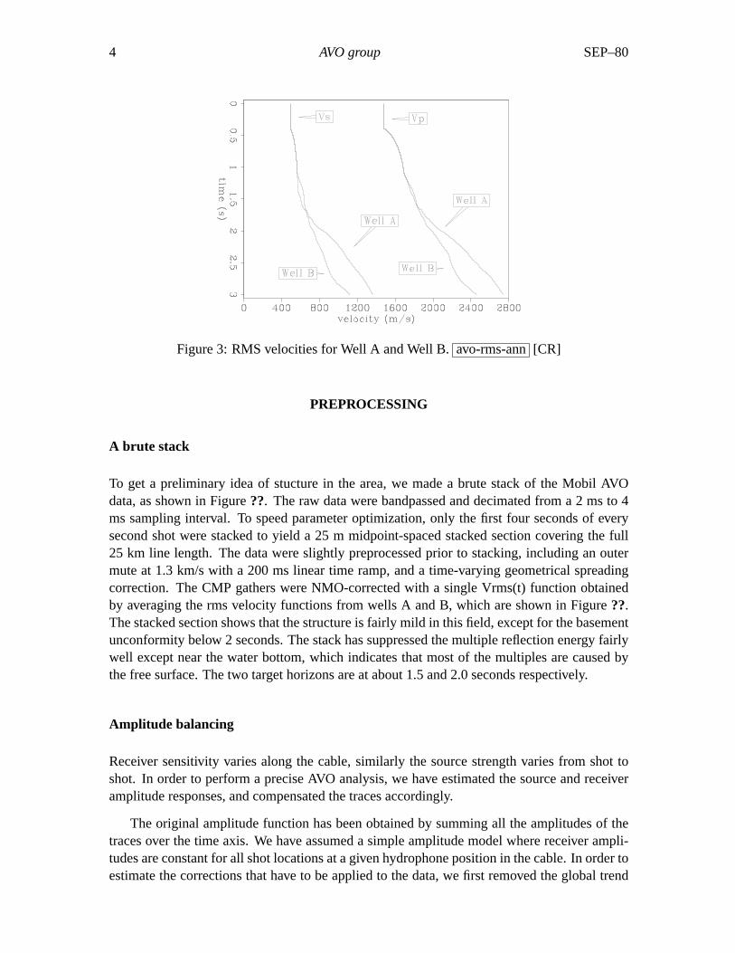
Converting the interval velocities to rms-velocities yielded the velocity functions shown inFigure 3. Within the first 2 seconds, the velocities obtained from well A and well B are fairlysimilar. At later times, the rms-velocities calculated for well B tend to be lower than thosefor well A. However, comparison with the interval velocities shows that the most significantdeviation occurs for the linearly interpolated values after 2.4 seconds. This indicates that thevelocities obtained by linear interpolation might be slightly underestimated.

The petrophysical data base indicates lithology and fluid content of both wells as a functionof depth. It contains the volume fractions of dry clay, bound water, coal, quartz, calcite,parallel pores, oil, gas, and water.


Figure 3: RMS velocities for Well A and Well B.avo-rms-ann[CR]

PREPROCESSING

A brute stack

To get a preliminary idea of stucture in the area, we made a brute stack of the Mobil AVOdata, as shown in Figure??. The raw data were bandpassed and decimated from a 2 ms to 4ms sampling interval. To speed parameter optimization, only the first four seconds of everysecond shot were stacked to yield a 25 m midpoint-spaced stacked section covering the full25 km line length. The data were slightly preprocessed prior to stacking, including an outermute at 1.3 km/s with a 200 ms linear time ramp, and a time-varying geometrical spreadingcorrection. The CMP gathers were NMO-corrected with a single Vrms(t) function obtainedby averaging the rms velocity functions from wells A and B, which are shown in Figure??.The stacked section shows that the structure is fairly mild in this field, except for the basementunconformity below 2 seconds. The stack has suppressed the multiple reflection energy fairlywell except near the water bottom, which indicates that most of the multiples are caused bythe free surface. The two target horizons are at about 1.5 and 2.0 seconds respectively.

Amplitude balancing

Receiver sensitivity varies along the cable, similarly the source strength varies from shot toshot. In order to perform a precise AVO analysis, we have estimated the source and receiveramplitude responses, and compensated the traces accordingly.

The original amplitude function has been obtained by summing all the amplitudes of thetraces over the time axis. We have assumed a simple amplitude model where receiver ampli-tudes are constant for all shot locations at a given hydrophone position in the cable. In order toestimate the corrections that have to be applied to the data, we first removed the global trend


Figure 4: A brute stack of the Mobil AVO dataset.avo-stack[CR]


in both receiver and shot directions. This was done by least-squares fitting a linear function inthe shot direction and the exponential of a quadratic function in the offset direction (Berliouxand Lumley, 1994).

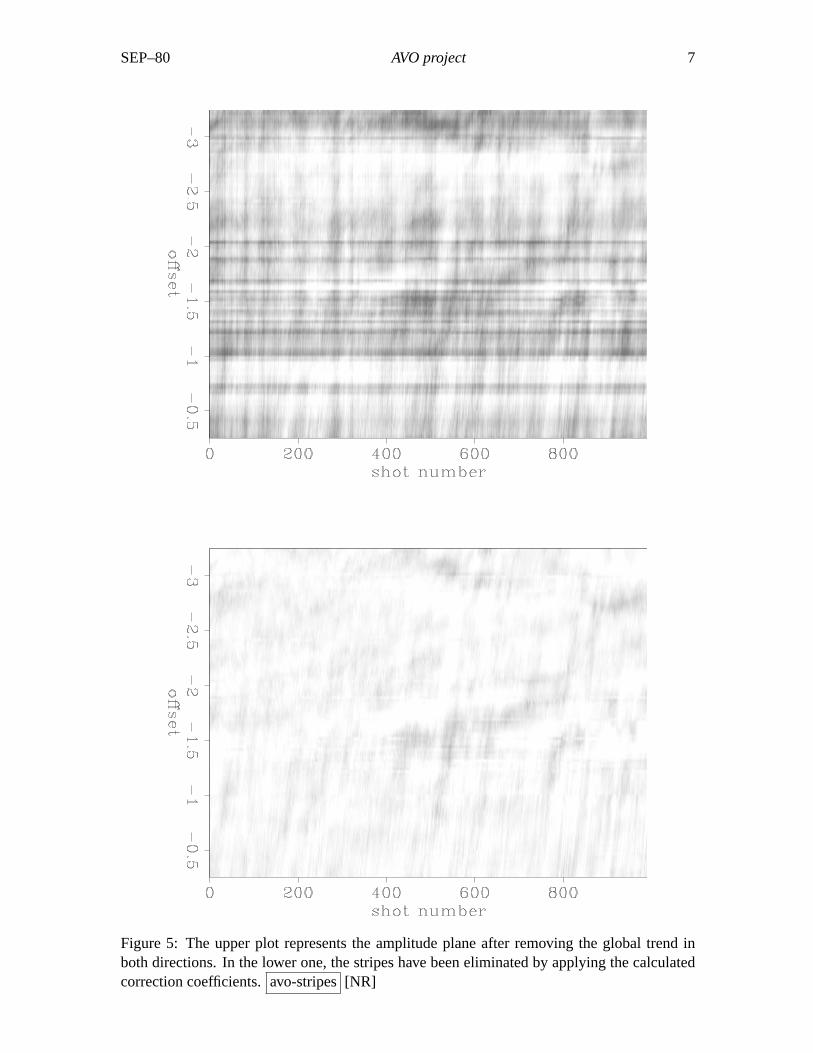
The upper plot in Figure 5 shows the amplitude plane after removal of the global trend.On the grey background, horizontal and vertical stripes are visible. The horizontal stripescorrespond to receivers stronger or weaker than the general tendency. The vertical stripescorrespond to varying pressure shots.

We have then estimated the correction coefficients by stacking the amplitude plane sepa-rately in both offset and shot direction after removal of the global trend. On the lower plotin Figure 5, the stripes have been eliminated by applying the correction coefficients in bothdirection.

MULTIPLE REFLECTIONS

One of the challenges of the Mobil AVO dataset is the presence of a large amount of multipleenergy on the prestack gathers, as indicated by the shot gather and velocity scan of Figure??. We intend to both 1) suppress multiple energy and recover primary reflection AVO re-sponses in order to perform AVO analysis, and 2) use the primary and multiple reflection datasimultaneously to measure and analyze AVO. Stew Levin has also urged Mobil to provide par-ticipants with a copy of their preprocessed data so that those interested in prestack inversioncan get rolling quickly, leaving the subject of multiples for concurrent research. We brieflydiscuss several avenues we are going to pursue.

Radon transform

From personal communication, we gather that Mobil has used a form of parabolic Radonfiltering (Hampson, 1986) with fair-to-good success in attenuating the multiple energy. Weare working with the ProMAX Radon Filter module to try to achieve a similar result. Currentlimitations of the ProMAX module are making tests on synthetic seismograms slow going.We are currently using a CSM SU utility to facilitate the split/merge functionality needed.

L2 velocity-transform pairs

We have much practical experience in computing stacking velocity scans, and can use that ex-pertise to optimally separate the multiple and primary reflection trends in velocity space. Thealgorithm that achieves the previous goal is the forward velocity transform. An example ofthe velocity transform space is shown in the scan of Figure??. Additionally, we have gainedsome insight in how to code adjoint and least-squares pseudo-inverse algorithms, given a for-ward transform code. We plan to use an enhanced forward velocity transform, its adjoint andits pseudo-inverse to suppress multiples while recovering primary reflection AVO amplitudes.


Figure 5: The upper plot represents the amplitude plane after removing the global trend inboth directions. In the lower one, the stripes have been eliminated by applying the calculatedcorrection coefficients.avo-stripes[NR]


This method builds upon previous work by Thorson (1984) and Harlan (1986), and can berelated to a generalized hyperbolic Radon transform multiple-suppression scheme.

Wave-equation multiple suppression

For the purpose of AVO analysis, perhaps the best tool for cleaning up prestack records con-taminated by multiples is the Delft surface-related multiple elimination algorithm of Verschuur(1991). We are developing the tools needed to implement this algorithm and, as discussed inthe next subsection, hope to employ them not just as a multiple suppression algorithm, butalso as an AVO estimation tool.

Migrating multiples

One of our goals is to apply the precept that multiples are data. We already know from Jon’sOverlay program (Claerbout, 1987) that multiple reflections can significantly increase the pre-cision of velocity and traveltime estimates for NMO. We also believe they can be used to in-crease the precision and reliability of amplitude versus angle (AVA) measurements on prestackdata. We think this can be accomplished by “migrating the multiples” as has been previouslysuggested at Delft (Berkhout, 1993) and the Colorado School of Mines (Zhdanov and Tjan,1993). We believe that the surface-related multiple elimination process can be adapted to buildan AVA estimate from free-surface multiple reflections. Even if such proves too grandiose forthe time frame of the project, the ability to suppress free-surface multiples is in itself a desir-able target. In another paper in this report, Yetmen Wang and Stew Levin develop and discusssome of the machinery they think is needed for this purpose.

MODELING

There are several reasons why we are interested in building depth models for the Mobil AVOdata. We will use the models to test our multiple suppression schemes in terms of recover-ing primary reflection AVO. We have constructed a 1-D elastic model in order to computea full-waveform elastic CMP gather with and without free-surface multiples. We have alsoconstructed an idealized 2-D depth model for generation of more sophisticated elastic finite-difference shot gather data. Finally, we would like to build a realistic 2-D depth model tocompute Kirchhoff Green’s functions for depth migration and to test wave-equation inversionschemes.

Haskell-Thompson 1-D modeling

We constructed a 1-D elastic model to test our multiple suppression methods. Each layer ischaracterized by the constant elastic parameters P-velocity, S-velocity and density, based onthe well-logs and the paper time-migrated section, which was provided by Mobil and is not


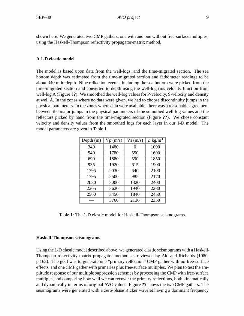
shown here. We generated two CMP gathers, one with and one without free-surface multiples,using the Haskell-Thompson reflectivity propagator-matrix method.

A 1-D elastic model

The model is based upon data from the well-logs, and the time-migrated section. The seabottom depth was estimated from the time-migrated section and fathometer readings to beabout 340 m in depth. Nine reflection events, including the sea bottom were picked from thetime-migrated section and converted to depth using the well-log rms velocity function fromwell-log A (Figure??). We smoothed the well-log values for P-velocity, S-velocity and densityat well A. In the zones where no data were given, we had to choose discontinuity jumps in thephysical parameters. In the zones where data were available, there was a reasonable agreementbetween the major jumps in the physical parameters of the smoothed well-log values and thereflectors picked by hand from the time-migrated section (Figure??). We chose constantvelocity and density values from the smoothed logs for each layer in our 1-D model. Themodel parameters are given in Table 1.

Depth (m) Vp (m/s) Vs (m/s) ρ kg/m3

340 1480 0 1000540 1780 550 1600690 1880 590 1850935 1920 615 19001395 2030 640 21001795 2500 985 21702030 3000 1320 24002265 3620 1940 22802560 3450 1840 2450— 3760 2136 2350

Table 1: The 1-D elastic model for Haskell-Thompson seismograms.

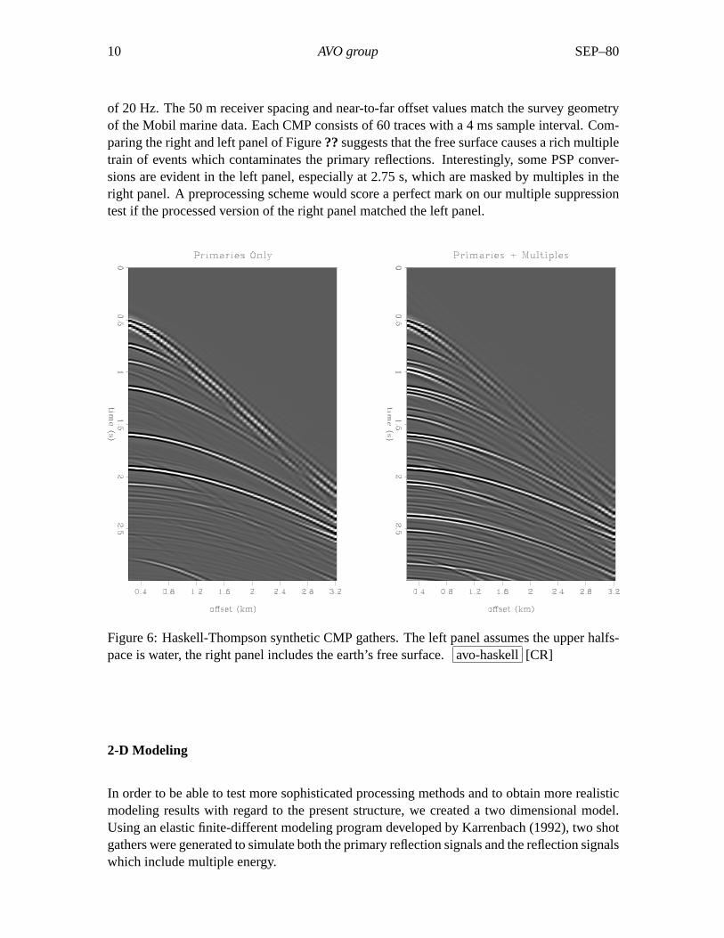
Haskell-Thompson seismograms

Using the 1-D elastic model described above, we generated elastic seismograms with a Haskell-Thompson reflectivity matrix propagator method, as reviewed by Aki and Richards (1980,p.163). The goal was to generate one “primary-reflection” CMP gather with no free-surfaceeffects, and one CMP gather with primaries plus free-surface multiples. We plan to test the am-plitude response of our multiple suppression schemes by processing the CMP with free-surfacemultiples and comparing how well we can recover the primary reflections, both kinematicallyand dynamically in terms of original AVO values. Figure??shows the two CMP gathers. Theseismograms were generated with a zero-phase Ricker wavelet having a dominant frequency


of 20 Hz. The 50 m receiver spacing and near-to-far offset values match the survey geometryof the Mobil marine data. Each CMP consists of 60 traces with a 4 ms sample interval. Com-paring the right and left panel of Figure??suggests that the free surface causes a rich multipletrain of events which contaminates the primary reflections. Interestingly, some PSP conver-sions are evident in the left panel, especially at 2.75 s, which are masked by multiples in theright panel. A preprocessing scheme would score a perfect mark on our multiple suppressiontest if the processed version of the right panel matched the left panel.

Figure 6: Haskell-Thompson synthetic CMP gathers. The left panel assumes the upper halfs-pace is water, the right panel includes the earth’s free surface.avo-haskell[CR]

2-D Modeling

In order to be able to test more sophisticated processing methods and to obtain more realisticmodeling results with regard to the present structure, we created a two dimensional model.Using an elastic finite-different modeling program developed by Karrenbach (1992), two shotgathers were generated to simulate both the primary reflection signals and the reflection signalswhich include multiple energy.


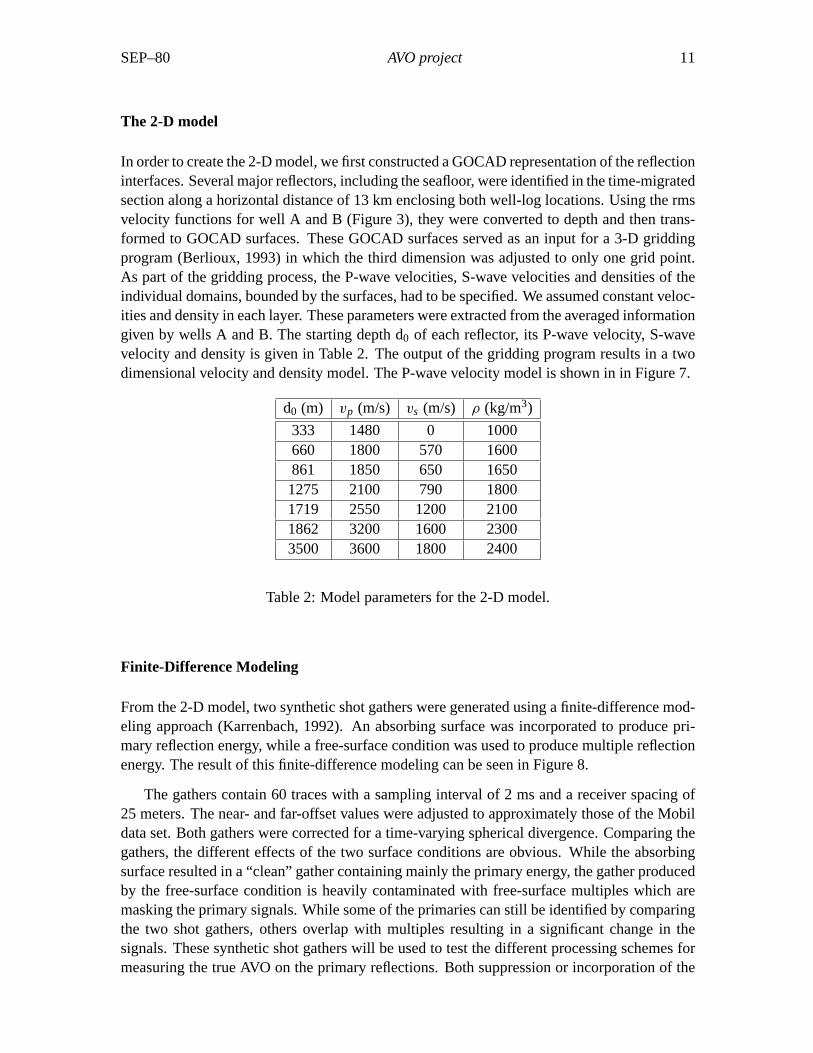
The 2-D model

In order to create the 2-D model, we first constructed a GOCAD representation of the reflectioninterfaces. Several major reflectors, including the seafloor, were identified in the time-migratedsection along a horizontal distance of 13 km enclosing both well-log locations. Using the rmsvelocity functions for well A and B (Figure 3), they were converted to depth and then trans-formed to GOCAD surfaces. These GOCAD surfaces served as an input for a 3-D griddingprogram (Berlioux, 1993) in which the third dimension was adjusted to only one grid point.As part of the gridding process, the P-wave velocities, S-wave velocities and densities of theindividual domains, bounded by the surfaces, had to be specified. We assumed constant veloc-ities and density in each layer. These parameters were extracted from the averaged informationgiven by wells A and B. The starting depth d0 of each reflector, its P-wave velocity, S-wavevelocity and density is given in Table 2. The output of the gridding program results in a twodimensional velocity and density model. The P-wave velocity model is shown in in Figure 7.

d0 (m) vp (m/s) vs (m/s) ρ (kg/m3)

333 1480 0 1000660 1800 570 1600861 1850 650 16501275 2100 790 18001719 2550 1200 21001862 3200 1600 23003500 3600 1800 2400

Table 2: Model parameters for the 2-D model.

Finite-Difference Modeling

From the 2-D model, two synthetic shot gathers were generated using a finite-difference mod-eling approach (Karrenbach, 1992). An absorbing surface was incorporated to produce pri-mary reflection energy, while a free-surface condition was used to produce multiple reflectionenergy. The result of this finite-difference modeling can be seen in Figure 8.

The gathers contain 60 traces with a sampling interval of 2 ms and a receiver spacing of25 meters. The near- and far-offset values were adjusted to approximately those of the Mobildata set. Both gathers were corrected for a time-varying spherical divergence. Comparing thegathers, the different effects of the two surface conditions are obvious. While the absorbingsurface resulted in a “clean” gather containing mainly the primary energy, the gather producedby the free-surface condition is heavily contaminated with free-surface multiples which aremasking the primary signals. While some of the primaries can still be identified by comparingthe two shot gathers, others overlap with multiples resulting in a significant change in thesignals. These synthetic shot gathers will be used to test the different processing schemes formeasuring the true AVO on the primary reflections. Both suppression or incorporation of the


Figure 7: 2-D P-wave velocity model in depth. The second layer is actually made of twoseparate layers with weak velocity contrast.avo-model [CR]

interfering multiple energy in the processing should produce the multiple-free synthetic shotgather from the one contaminated with multiples.

AVO ANALYSIS

After careful true-amplitude preprocessing and multiple suppression, the data will be suitablefor AVO analysis and impedance inversion. Subsequently, we will try to relate the estimatedseismic parameters to lithology and pore fluid content by developing AVO indicators in con-junction with rock physics analysis and the Mobil petrophysical database. The simplest ap-proach is to first perform a linearized parameter inversion on unmigrated amplitude-correctedCMP gathers. Ecker and Lumley (1993;?) showed an example of this on methane hydrateAVO data. In a more sophisticated analysis, a Kirchhoff wave-equation elastic impedance in-version will be attempted. The basis of this technique was described by Lumley and Beydoun(1991), and was applied in a gas reservoir study by Lumley (1993) and in a recent methanehydrate analysis by Ecker and Lumley (1994). Since the field structure is not complicated, wealso expect to make a meaningful comparison of time and depth migration/inversion resultson the Mobil data. Another approach is to analyze the angle-dependent reflectivity image ob-tained by imaging with wavefront synthesis. This technique was described by Ji (1993) andwas tested on the Marmousi dataset. Unlike the Marmousi data, the simple structure on theMobil data should provide more interpretable angle-dependent reflectivity image.


Figure 8: Finite-difference synthetic shot gathers for the 2-D model. The left gather assumedan absorbing boundary condition, while the right gather incorporated a free-surface condition.avo-findiff [CR]


SUMMARY

In summary, we have given an overview of our AVO project, from preliminary results toplanned research strategy. We expect to participate in Mobil’s AVO review workshop in Lon-don this summer, and at the special SEG AVO workshop in Los Angeles this October. We planto harness our combined technical skills and field-data expertise in order to solve some of thechallenging problems presented in the Mobil AVO dataset as part of an ongoing SEP project.

ACKNOWLEDGMENTS

We would like to thank Bob Keys of the Mobil Exploration and Production Technical Centerfor providing SEP with the Mobil AVO dataset, and visiting us to discuss our mutual AVOresearch interests.

REFERENCES

Berkhout, A. J., 1993, Migration of multiple reflections: 63rd Ann. Mtg. and Intl. Expo., Soc.Expl. Geophys., Expanded Abstracts, 1022–1025.

Berlioux, A., and Lumley, D., 1994, Amplitude balancing for AVO analysis: SEP–80, 345–356.

Berlioux, A., 1993, 3-D grid with GOCAD: SEP–79, 301–318.

Claerbout, J. F., 1987, Interpretation with the overlay program: SEP–51, 269–300.

Ecker, C., and Lumley, D., 1993, AVO analysis of methane hydrate seismic data: SEP–79,161–176.

Ecker, C., and Lumley, D. E., 1994, Seismic AVO analysis of methane hydrate structures:SEP–80, ??–??.

Hampson, D., 1986, Inverse velocity stacking for multiple elimination: J. Can. Soc. Expl.Geophys.,22, no. 1, 44–55.

Harlan, W. S., 1986, Signal-noise separation and seismic inversion: Ph.D. thesis, StanfordUniversity.

Ji, J., 1993, Controlled illumination by wavefront synthesis: SEP–79, 129–144.

Karrenbach, M., 1992, “Plug ’n Play” wave equation modules: SEP–75, 273–288.

Lumley, D., and Beydoun, W., 1991, Elastic parameter estimation by Kirchhoff prestack depthmigration inversion: SEP–70, 165–192.


Lumley, D. E., 1993, Kirchhoff prestack impedance inversion: a gas reservoir pilot study:SEP–77, 211–230.

Ostrander, W. J., 1984, Plane-wave reflection coefficients for gas sands at nonnormal anglesof incidence: Geophysics,49, 1637–1649.

Thorson, J. R., 1984, Velocity stack and slant stack inversion methods: Ph.D. thesis, StanfordUniversity.

Verschuur, D. J., Berkhout, A. J., and Wapenaar, C. P. A., 1991, Surface-related multipleelimination: Application on real data: 61st Annual Internat. Mtg., Soc. Expl. Geophys.,Expanded Abstracts, 1476–1479.

Zhdanov, M. S., and Tjan, T., 1993, Migration by analytic continuation through a variablebackground medium: 63rd Ann. Mtg. and Intl. Expo., Soc. Expl. Geophys., Expanded Ab-stracts, 1048–1051.

An AVO analysis project - Stanford · PDF file2 AVO group SEP–80 In this paper we present the Mobil AVO data set and describe our preliminary preprocess-ing work. We discuss model

Documents