An automation system for gas-lifted oil wells: Model identification, control, and optimization

Journal of Petroleum Science and Engineering 70 (2010) 157–167

Contents lists available at ScienceDirect

Journal of Petroleum Science and Engineering

j ourna l homepage: www.e lsev ie r.com/ locate /pet ro l

Research paper

An automation system for gas-lifted oil wells: Model identification, control,and optimization

Eduardo Camponogara a,⁎,1, Agustinho Plucenio a,2, Alex F. Teixeira b, Sthener R.V. Campos b

a Department of Automation and Systems Engineering, Federal University of Santa Catarina, Cx.P. 476, 88040-900 Florianópolis, SC, Brazilb Petrobras Research Center, Cidade Universitária Q.7 Ilha do Fundão, 21.949-900 Rio de Janeiro, RJ, Brazil

⁎ Corresponding author.E-mail address: [email protected] (E. Campono

1 Supported by CNPq (Brazil) under grants #306398/2 Supported by Agência Nacional do Petróleo, Gás Na

under grant PRH-34/aciPG/ANP.

0920-4105/$ – see front matter © 2009 Elsevier B.V. Aldoi:10.1016/j.petrol.2009.11.003

a b s t r a c t

Article history:Received 6 June 2008Accepted 4 November 2009

Keywords:smart fieldsgas-lifted wellssystem automationcontroloptimization

Smart fields technology advocates the use of a suite of skills, workflows, and technologies to drive efficiencygains while maximizing oil recovery from reservoirs. This paper contributes to smart fields technology bydeveloping an automation system for integrated operation of gas-lift platforms, thereby bridging the gapbetween downhole devices (sensors, valves, and controllers) and surface facilities (operating policies,constraints, and faults). The components of the system are: (1) a module for identification of well-performance curves from downhole pressure measurements; (2) a control strategy for the pressure of thegas-lift manifold and a software sensor to indirectly measure the gas-mass flow-rate available for artificiallifting; and (3) an algorithm for optimal allocation of limited resources, such as the lift-gas rate, fluidhandling capacities, and water-treatment processing capacity. The paper reports results from simulationsperformed with a prototype platform as a proof of concept.

gara).2003-6 and #479157/2006-5.tural e Biocombustíveis (ANP)

l rights reserved.

© 2009 Elsevier B.V. All rights reserved.

1. Introduction

The growing demand for fossil fuels is compelling the oil industryto operate oil fields in more innovative ways (DeVries, 2005; Murrayet al., 2006). To match the challenge, the smart fields technology isemploying a suite of skills, workflows, and technologies to optimizeproduction of oil fields in the long run (Williams and Webb, 2007).

The first applications of smart fields were limited to simple auto-mation back in the late 1960s. Today, such applications are regardedas smartwells,meaning thedesignof completionswithdownhole equip-ment forflow control and sensors thatmeasure pressure, temperature,and flow (Williams andWebb, 2007). Data from the sensors are trans-mitted to surface facilities, providing useful information for monitor-ing the reservoir and optimizing production.

Recent studies confirm that smart wells help improve oil recovery,reduce interventions, and control byproducts such as water (Bogaertet al., 2004). The findings indicate that automation systems should gobeyond the wells to encompass surface facilities. However, the devel-opment of such systems is a formidable challenge, entailing the designof sensors, information systems, and control and optimization algo-rithms of considerable complexity. This technology is known as smartfields, i-fields, field of the future, and digital integrated field manage-ment (GeDIg) (Plucenio and Pagano, 2004; Moisés et al., 2008).

Oil companies view smart fields as an evolving technology thatif materialized will bring great benefits while, on the other hand,research groups see this trend as an opportunity for advancing scienceand technology. Progress has been made in a number of fronts, in-cluding sensors (Nath et al., 2006; Aref et al., 2006), frameworks fordata acquisition (DeVries, 2005), and studies on reservoir optimiza-tion (Yeten and Jalali, 2001; Yeten et al., 2004).

This paper contributes to smart fields technology by developingan automation system for integrated operation of gas-lift platforms,thereby bridging the gap between smart downhole devices (sensors,valves, and controllers) and surface facilities. The automation system hasthree modules.

The first module consists of algorithms for estimating the well-performance curve (WPC) of gas-lifted wells from downhole pressuremeasurements. The algorithms obtain accurate WPCs despite using alimited number of data points around the lowest well-flowing pres-sure point, incurring little reduction on production.

The second module consists of a control-based sensor for estimat-ing the available gas-mass flow-rate supplied by the compressingstation to the gas-lift manifold (GLM). The available gas-mass flow-rateis informed to eachwell gas-injection flow-rate controllerwhich is usedto derive its set-point.

The third module consists of algorithms that distribute the availablelift-gas rate to thewells, relying on theirWPCs and accounting for otherfacility constraints. The models and algorithms yield provably optimalallocations of the limited resources.

The paper is structured as follows. Section 2 gives an overview of theautomation system, develops an algorithm for identification of the inflowproduction relationship (IPR) from well-flowing pressure measurements,

158 E. Camponogara et al. / Journal of Petroleum Science and Engineering 70 (2010) 157–167

andproposes a control algorithmfor theGLM. Section3 formalizes the lift-gas allocation problem under multiple facility constraints, deliversa mixed-integer reformulation by piecewise linearizing the WPCs, andproposes an efficient cut-and-branch algorithm. Section 4 coalesces thesedevelopments in a prototype platform of the automation system,reporting results from a case study as a proof of concept.

2. An automatic control system for gas-lift operations

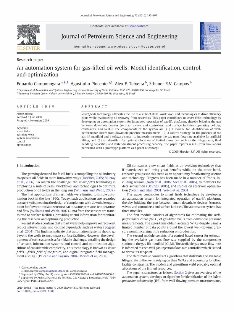
This section proposes models and control algorithms to operate agroup of wells equipped with downhole pressure and temperaturesensors. Each well has a local controller for the lift-gas flow suppliedby a common manifold as shown in Fig. 1. Downhole pressure andtemperature measurements are not only interesting from the oper-ations point of view, but they also provide useful information formanagement and oil recovery of the oil field.

The automation system should operate the gas-lifted wells opti-mally under conditions of high availability of lift-gas, while ensuringstable operations during periods of shortage. State-of-the-art opti-mization algorithms that yield an optimal operation are proposed inSection 3. As these algorithms rely on well performance curves andthe available gas-injection flow-rate, this section develops a practicalprocedure to obtain WPCs from downhole pressure measurementsand a control-based algorithm to estimate the available gas-massflow-rate of lift-gas.

2.1. Obtaining the WPC curves

Despite all the progress on the technology for multiphase flow-rate measurement, such instruments are not currently used in everyproducing well due to the high cost, the difficulty of installation inexisting wells, and their limited accuracy which sometimes is belowstandards set by regulatory agencies. For these reasons, the methodof aligning a well to a test separator is still widely used for a reliablemeasurement of the oil, gas and water flow-rate.

The industry has relied on inflow production relationships torelate the well liquid flow-rate and the pressure in front of theperforated zone. Several models were developed for saturated andunder-saturated fluid production. Since IPR curves change slowly overtime for most of the wells, they were seldom updated by means ofproduction tests in the absence of downhole pressure sensors.

Permanent downhole pressure and temperature sensors allow theoperator to perform production tests more frequently by directingthe well production to a test separator. Such instruments facilitateacquisition and processing of separation test data, thereby obtaininga more accurate IPR curve and well production parameters such aswater saturation (BSW) and gas–oil ratio (GOR). With downhole pres-sure measurements, the oil, water, and gas flow-rate can be estimatedfrom equations. For under-saturated reservoir (formation pressureabove the bubble point pressure), the equation for the oil flow-rate is:

qo = Jðp�−pwf Þ; ð1Þ

Fig. 1. Gas-lift manifold.

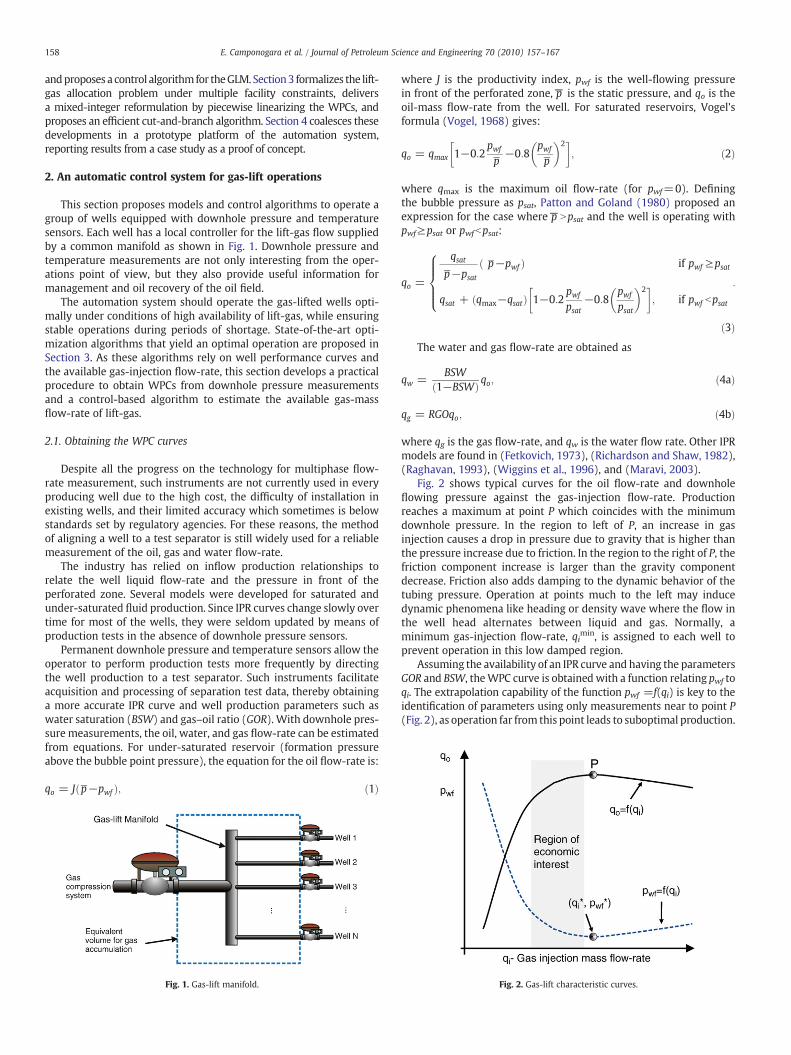
where J is the productivity index, pwf is the well-flowing pressurein front of the perforated zone, p is the static pressure, and qo is theoil-mass flow-rate from the well. For saturated reservoirs, Vogel'sformula (Vogel, 1968) gives:

qo = qmax 1−0:2pwf

p� −0:8pwf

p�� �2� �

; ð2Þ

where qmax is the maximum oil flow-rate (for pwf=0). Definingthe bubble pressure as psat, Patton and Goland (1980) proposed anexpression for the case where p Npsat and the well is operating withpwf≥psat or pwfbpsat:

qo =

qsatp�−psat

ð p�−pwf Þ if pwf ≥psat

qsat + ðqmax−qsatÞ 1−0:2pwf

psat−0:8

pwf

psat

� �2� �; if pwf bpsat

:

8>>><>>>:

ð3ÞThe water and gas flow-rate are obtained as

qw =BSW

ð1−BSWÞ qo; ð4aÞ

qg = RGOqo; ð4bÞ

where qg is the gas flow-rate, and qw is the water flow rate. Other IPRmodels are found in (Fetkovich, 1973), (Richardson and Shaw, 1982),(Raghavan, 1993), (Wiggins et al., 1996), and (Maravi, 2003).

Fig. 2 shows typical curves for the oil flow-rate and downholeflowing pressure against the gas-injection flow-rate. Productionreaches a maximum at point P which coincides with the minimumdownhole pressure. In the region to left of P, an increase in gasinjection causes a drop in pressure due to gravity that is higher thanthe pressure increase due to friction. In the region to the right of P, thefriction component increase is larger than the gravity componentdecrease. Friction also adds damping to the dynamic behavior of thetubing pressure. Operation at points much to the left may inducedynamic phenomena like heading or density wave where the flow inthe well head alternates between liquid and gas. Normally, aminimum gas-injection flow-rate, qimin, is assigned to each well toprevent operation in this low damped region.

Assuming the availability of an IPR curve and having the parametersGOR and BSW, theWPC curve is obtained with a function relating pwf toqi. The extrapolation capability of the function pwf =f(qi) is key to theidentification of parameters using only measurements near to point P(Fig. 2), as operation far from this point leads to suboptimal production.

Fig. 2. Gas-lift characteristic curves.

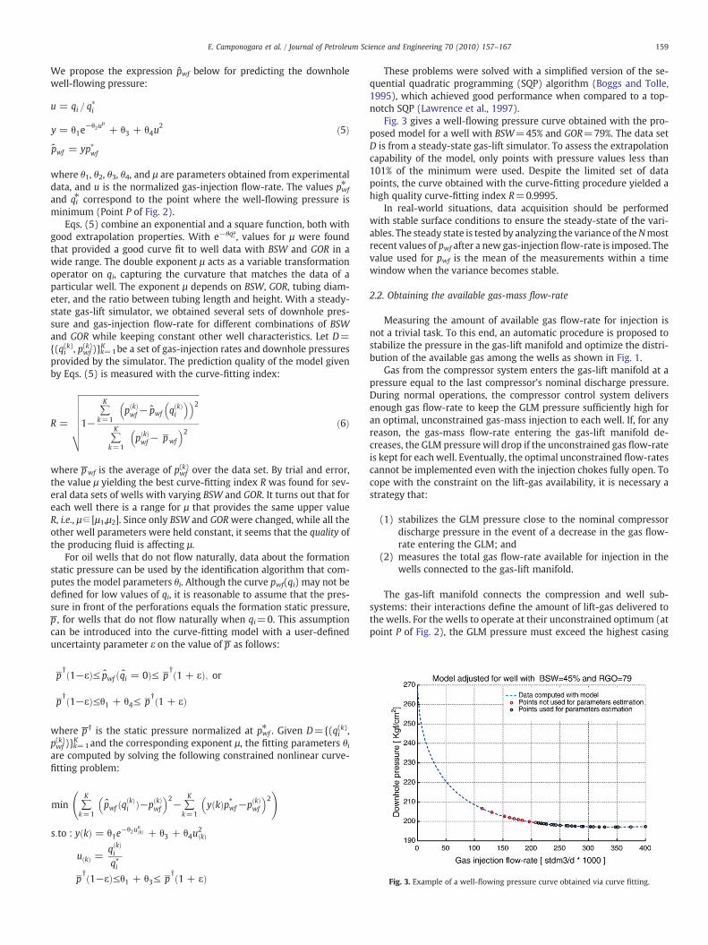
Fig. 3. Example of a well-flowing pressure curve obtained via curve fitting.

159E. Camponogara et al. / Journal of Petroleum Science and Engineering 70 (2010) 157–167

We propose the expression pwf below for predicting the downholewell-flowing pressure:

u = qi = q⁎i

y = θ1e−θ2u

μ

+ θ3 + θ4u2

pwf = yp⁎wf

ð5Þ

where θ1, θ2, θ3, θ4, and µ are parameters obtained from experimentaldata, and u is the normalized gas-injection flow-rate. The values pwf

⁎

and qi⁎ correspond to the point where the well-flowing pressure isminimum (Point P of Fig. 2).

Eqs. (5) combine an exponential and a square function, both withgood extrapolation properties. With e−θqi

µ, values for µ were found

that provided a good curve fit to well data with BSW and GOR in awide range. The double exponent µ acts as a variable transformationoperator on qi, capturing the curvature that matches the data of aparticular well. The exponent µ depends on BSW, GOR, tubing diam-eter, and the ratio between tubing length and height. With a steady-state gas-lift simulator, we obtained several sets of downhole pres-sure and gas-injection flow-rate for different combinations of BSWand GOR while keeping constant other well characteristics. Let D={(qi

(k), pwf(k))}k=1

K be a set of gas-injection rates and downhole pressuresprovided by the simulator. The prediction quality of the model givenby Eqs. (5) is measured with the curve-fitting index:

R =

ffiffiffiffiffiffiffiffiffiffiffiffiffiffiffiffiffiffiffiffiffiffiffiffiffiffiffiffiffiffiffiffiffiffiffiffiffiffiffiffiffiffiffiffiffiffiffiffiffiffiffiffiffiffiffiffiffiffiffiffi1−

∑K

k=1pðkÞwf− pwf qðkÞi

� �� �2∑K

k=1pðkÞwf− p�wf

� �2

vuuuuuut ð6Þ

where pwf is the average of pwf(k) over the data set. By trial and error,

the value µ yielding the best curve-fitting index R was found for sev-eral data sets of wells with varying BSW and GOR. It turns out that foreach well there is a range for µ that provides the same upper valueR, i.e., µ∈ [µ1,µ2]. Since only BSW and GORwere changed, while all theother well parameters were held constant, it seems that the quality ofthe producing fluid is affecting µ.

For oil wells that do not flow naturally, data about the formationstatic pressure can be used by the identification algorithm that com-putes the model parameters θi. Although the curve pwf(qi) may not bedefined for low values of qi, it is reasonable to assume that the pres-sure in front of the perforations equals the formation static pressure,p , for wells that do not flow naturally when qi=0. This assumptioncan be introduced into the curve-fitting model with a user-defineduncertainty parameter ε on the value of p as follows:

p�†ð1−εÞ≤ pwf ðqi = 0Þ≤ p�†ð1 + εÞ; or

p�†ð1−εÞ≤θ1 + θ4≤ p�†ð1 + εÞ

where p † is the static pressure normalized at pwf⁎ . Given D={(qi

(k),pwf(k))}k=1

K and the corresponding exponent µ, the fitting parameters θiare computed by solving the following constrained nonlinear curve-fitting problem:

min ∑K

k=1pwf ðqðkÞi Þ−pðkÞwf

� �2−∑K

k=1yðkÞp4wf−pðkÞwf

� �2 !

s:to : yðkÞ = θ1e−θ2u

ukð Þ + θ3 + θ4u

2kð Þ

u kð Þ =qðkÞi

q4ip�†ð1−εÞ≤θ1 + θ3≤ p�†ð1 + εÞ

These problems were solved with a simplified version of the se-quential quadratic programming (SQP) algorithm (Boggs and Tolle,1995), which achieved good performance when compared to a top-notch SQP (Lawrence et al., 1997).

Fig. 3 gives a well-flowing pressure curve obtained with the pro-posed model for a well with BSW=45% and GOR=79%. The data setD is from a steady-state gas-lift simulator. To assess the extrapolationcapability of the model, only points with pressure values less than101% of the minimum were used. Despite the limited set of datapoints, the curve obtained with the curve-fitting procedure yielded ahigh quality curve-fitting index R=0.9995.

In real-world situations, data acquisition should be performedwith stable surface conditions to ensure the steady-state of the vari-ables. The steady state is tested by analyzing the variance of theNmostrecent values of pwf after a new gas-injection flow-rate is imposed. Thevalue used for pwf is the mean of the measurements within a timewindow when the variance becomes stable.

2.2. Obtaining the available gas-mass flow-rate

Measuring the amount of available gas flow-rate for injection isnot a trivial task. To this end, an automatic procedure is proposed tostabilize the pressure in the gas-lift manifold and optimize the distri-bution of the available gas among the wells as shown in Fig. 1.

Gas from the compressor system enters the gas-lift manifold at apressure equal to the last compressor's nominal discharge pressure.During normal operations, the compressor control system deliversenough gas flow-rate to keep the GLM pressure sufficiently high foran optimal, unconstrained gas-mass injection to each well. If, for anyreason, the gas-mass flow-rate entering the gas-lift manifold de-creases, the GLM pressure will drop if the unconstrained gas flow-rateis kept for each well. Eventually, the optimal unconstrained flow-ratescannot be implemented even with the injection chokes fully open. Tocope with the constraint on the lift-gas availability, it is necessary astrategy that:

(1) stabilizes the GLM pressure close to the nominal compressordischarge pressure in the event of a decrease in the gas flow-rate entering the GLM; and

(2) measures the total gas flow-rate available for injection in thewells connected to the gas-lift manifold.

The gas-lift manifold connects the compression and well sub-systems: their interactions define the amount of lift-gas delivered tothe wells. For the wells to operate at their unconstrained optimum (atpoint P of Fig. 2), the GLM pressure must exceed the highest casing

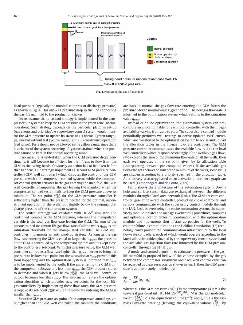
Fig. 4. Pressure in the gas-lift manifold.

160 E. Camponogara et al. / Journal of Petroleum Science and Engineering 70 (2010) 157–167

head pressure (typically the nominal compressor discharge pressure)as shown in Fig. 4. This allows a pressure drop in the line connectingthe gas-lift manifold to the production chokes.

Let us assume that a control strategy is implemented in the com-pressor subsystem to keep the GLM pressure in the green zone (normaloperation). Such strategy depends on the particular platform set-up(gas clients and priorities). A supervisory control system would moni-tor the GLM pressure to update its status to (i) normal (green range),(ii) normal without test (yellow range), and (iii) constrained operation(red range). Tests should not be allowed in the yellow range, since thereis a chance of the system becoming lift-gas constrained when the pres-sure cannot be kept in the normal operating range.

If no measure is undertaken when the GLM pressure drops con-tinually, it will become insufficient for the lift-gas to flow from theGLM to the casing heads. Obviously an action has to be taken beforethat happens. Our strategy implements a second GLM pressure con-troller (GLM well controller) which disputes the control of the GLMpressure with the compressor control system: while the compres-sor control system actuates in the gas entering the manifold, the GLMwell controller manipulates the gas leaving the manifold when thecompressor control system fails to keep the GLM pressure above itsminimum. The set point pGLM

min for the GLM pressure controller issufficiently higher than the pressure needed for the optimal, uncon-strained operation of the wells, but slightly below the nominal dis-charge pressure of the compressor system.

The control strategy was validated with OLGA® simulator. Thecontrolled variable is the GLM pressure, whereas the manipulatedvariable is the total gas flow-rate leaving the GLM. The sum of theunconstrained maximum lift-gas flow-rate of all the wells, qtotal, is thesaturation threshold for the manipulated variable. The GLM wellcontroller implements an anti wind-up strategy. As long as the gasflow-rate entering the GLM is equal or larger than qtotal, the pressureat the GLM is controlled by the compressor system and it is kept closeto the controller's set-point. With this pressure value, the GLM wellcontroller computes a flow-rate higher than qtotal in order to bring thepressure to its lower set-point, but the saturation at qtotal prevents thisfrom happening and the optimization system is informed that qtotalis to be implemented by the wells. If the gas entering the GLM fromthe compressor subsystem is less than qtotal, the GLM pressure startsto decrease and when it gets below pGLM

min , the GLM well controlleroutput becomes less than qtotal. This information enters the optimi-zation algorithm which provides new set-points for the local lift-gas controllers. By implementing these flow-rates, the GLM pressureis kept at its set-point pGLMmin while the flow-rate entering the GLM issmaller than qtotal.

Since the GLM pressure set-point of the compressor control systemis higher than the GLM well controller, the moment the conditions

are back to normal, the gas flow-rate entering the GLM forces thepressure back to normal values (green zone). The new gas flow-rate isinformed to the optimization system which returns to the saturationvalue qtotal.

Instead of online optimization, the automation system can pre-compute an allocation table for each local controller with the lift-gasavailability varying from zero to qtotal. The supervisory control moduleperiodically performs well testings to derive updated WPC curves,which are transferred to the optimization system to revise and uploadthe allocation tables in the lift-gas flow-rate controllers. The GLMpressure controller communicates the available flow-rate to the localwell controllers which respond accordingly. If the available gas flow-rate exceeds the sum of the minimum flow-rate of all the wells, theneach well operates at the set-point given by its allocation table(interpolating between pre-computed values). If the available gasflow-rate gets below the sum of theminimum of thewells, somewellsare shut-in according to a priority specified in the allocation table.Alternatively, a strategy based on an activation precedence graph canbe used (Camponogara and de Conto, 2009).

Fig. 5 shows the architecture of the automation system. Down-hole and surface sensor data are exchanged between the differentmodules through a local area network (LAN). The GLM pressure con-troller, gas-lift flow-rate controller, production choke controller, andsensors communicate with the supervisory control module throughthe LAN. Besides overseeing the entire automation system, the super-visorymodule initiates andmanageswell testingprocedures, computesand uploads allocation tables in coordination with the optimizationmodule, and implements shut-in/start-up policies for the wells. Tocounter failure in communications, the Fieldbus Foundation (FF) tech-nology could provide the communication infrastructure to the localflow-rate controllers, each of which would operate according to thelatest allocation table uploaded by the supervisory control system andthe available gas-injection flow-rate informed by the GLM pressurecontroller through the FF H1 bus.

A model and control algorithm to estimate the pressure in the gas-lift manifold is proposed below. If the volume occupied by the gasbetween the compressor subsystem and each well control valve canbe regarded as a gas reservoir, as shown in Fig. 1, then the GLM pres-sure is approximately modeled by:

∂p∂t =

RTMV

ðqe−qsÞ ð7Þ

where: p is the GLM pressure (Pa); T is the temperature (K); R is theuniversal gas constant (8:3144126 Pam3mol

K); M is the gas molecular

weight Kgmol

� �; V is the equivalent volume (m3); and qe (qs) is the gas-

mass flow-rate entering (leaving) the equivalent volume Kgs

� �. By

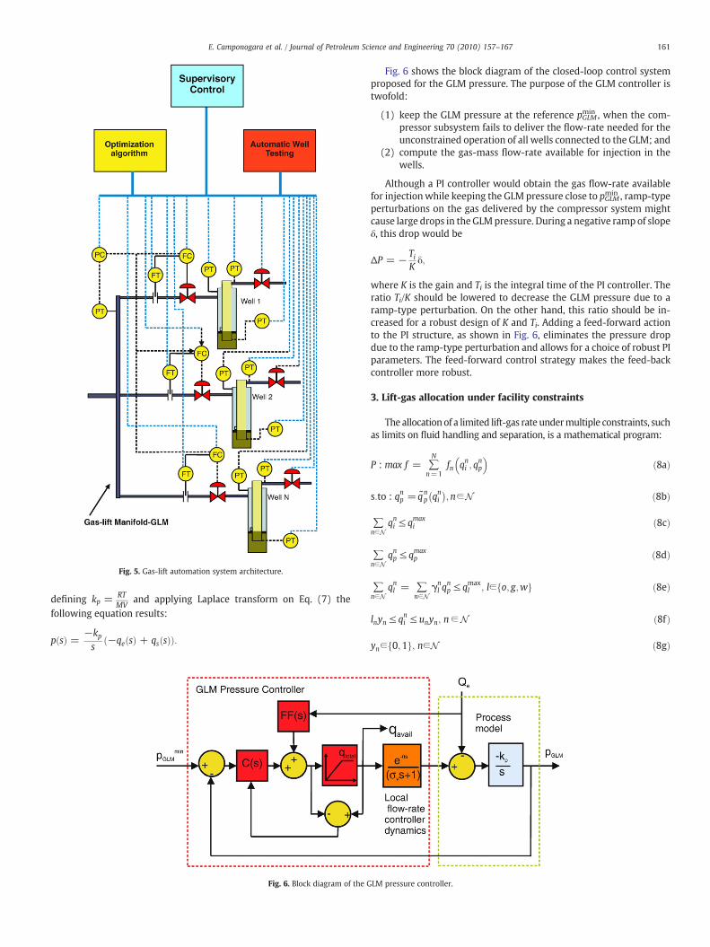
Fig. 5. Gas-lift automation system architecture.

161E. Camponogara et al. / Journal of Petroleum Science and Engineering 70 (2010) 157–167

defining kp = RTMV

and applying Laplace transform on Eq. (7) thefollowing equation results:

pðsÞ = −kps

ð−qeðsÞ + qsðsÞÞ:

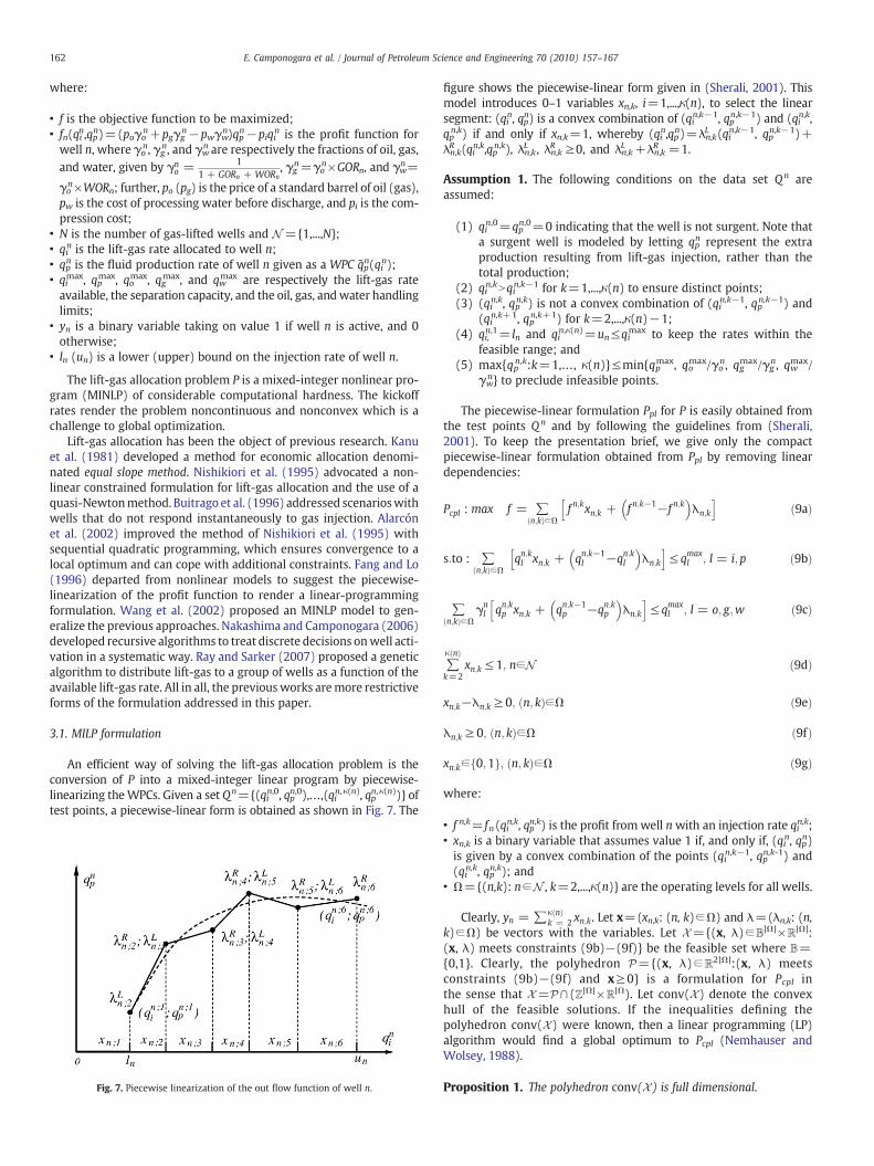
Fig. 6. Block diagram of the G

Fig. 6 shows the block diagram of the closed-loop control systemproposed for the GLM pressure. The purpose of the GLM controller istwofold:

(1) keep the GLM pressure at the reference pGLMmin , when the com-

pressor subsystem fails to deliver the flow-rate needed for theunconstrained operation of all wells connected to the GLM; and

(2) compute the gas-mass flow-rate available for injection in thewells.

Although a PI controller would obtain the gas flow-rate availablefor injectionwhile keeping the GLM pressure close to pGLM

min , ramp-typeperturbations on the gas delivered by the compressor system mightcause large drops in the GLMpressure. During a negative ramp of slopeδ, this drop would be

ΔP = − TiKδ;

where K is the gain and Ti is the integral time of the PI controller. Theratio Ti/K should be lowered to decrease the GLM pressure due to aramp-type perturbation. On the other hand, this ratio should be in-creased for a robust design of K and Ti. Adding a feed-forward actionto the PI structure, as shown in Fig. 6, eliminates the pressure dropdue to the ramp-type perturbation and allows for a choice of robust PIparameters. The feed-forward control strategy makes the feed-backcontroller more robust.

3. Lift-gas allocation under facility constraints

The allocationof a limited lift-gas rate undermultiple constraints, suchas limits on fluid handling and separation, is a mathematical program:

P : max f = ∑N

n=1fn qni ; q

np

� �ð8aÞ

s:to : qnp = qnp qni

;n∈N ð8bÞ

∑n∈N

qni ≤ qmaxi ð8cÞ

∑n∈N

qnp ≤ qmaxp ð8dÞ

∑n∈N

qnl = ∑n∈N

γnl q

np ≤ qmax

l ; l∈fo; g;wg ð8eÞ

lnyn ≤ qni ≤ unyn; n∈N ð8fÞ

yn∈f0;1g; n∈N ð8gÞ

LM pressure controller.

162 E. Camponogara et al. / Journal of Petroleum Science and Engineering 70 (2010) 157–167

where:

• f is the objective function to be maximized;• fn(qin,qpn)=(poγo

n+pgγgn−pwγw

n)qpn−piqin is the profit function for

well n, where γon, γg

n, and γwn are respectively the fractions of oil, gas,

and water, given by γno = 1

1 + GORn + WORn, γgn=γon×GORn, and γwn=

γon×WORn; further, po (pg) is the price of a standard barrel of oil (gas),pw is the cost of processing water before discharge, and pi is the com-pression cost;

• N is the number of gas-lifted wells and N ={1,...,N};• qi

n is the lift-gas rate allocated to well n;• qp

n is the fluid production rate of well n given as a WPC qpn(qin);

• qimax, qpmax, qomax, qgmax, and qw

max are respectively the lift-gas rateavailable, the separation capacity, and the oil, gas, andwater handlinglimits;

• yn is a binary variable taking on value 1 if well n is active, and 0otherwise;

• ln (un) is a lower (upper) bound on the injection rate of well n.

The lift-gas allocation problem P is a mixed-integer nonlinear pro-gram (MINLP) of considerable computational hardness. The kickoffrates render the problem noncontinuous and nonconvex which is achallenge to global optimization.

Lift-gas allocation has been the object of previous research. Kanuet al. (1981) developed a method for economic allocation denomi-nated equal slope method. Nishikiori et al. (1995) advocated a non-linear constrained formulation for lift-gas allocation and the use of aquasi-Newtonmethod. Buitrago et al. (1996) addressed scenarioswithwells that do not respond instantaneously to gas injection. Alarcónet al. (2002) improved the method of Nishikiori et al. (1995) withsequential quadratic programming, which ensures convergence to alocal optimum and can cope with additional constraints. Fang and Lo(1996) departed from nonlinear models to suggest the piecewise-linearization of the profit function to render a linear-programmingformulation. Wang et al. (2002) proposed an MINLP model to gen-eralize the previous approaches. Nakashima and Camponogara (2006)developed recursive algorithms to treat discrete decisions onwell acti-vation in a systematic way. Ray and Sarker (2007) proposed a geneticalgorithm to distribute lift-gas to a group of wells as a function of theavailable lift-gas rate. All in all, the previousworks aremore restrictiveforms of the formulation addressed in this paper.

3.1. MILP formulation

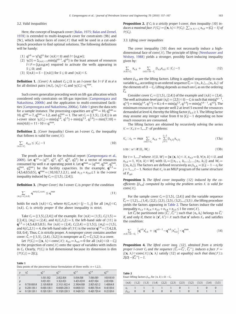
An efficient way of solving the lift-gas allocation problem is theconversion of P into a mixed-integer linear program by piecewise-linearizing theWPCs. Given a set Qn={(qin,0, qpn,0),…,(qin,κ(n), qpn,κ(n))} oftest points, a piecewise-linear form is obtained as shown in Fig. 7. The

Fig. 7. Piecewise linearization of the out flow function of well n.

figure shows the piecewise-linear form given in (Sherali, 2001). Thismodel introduces 0–1 variables xn,k, i=1,...,κ(n), to select the linearsegment: (qin, qpn) is a convex combination of (qin,k−1, qpn,k−1) and (qin,k,qpn,k) if and only if xn,k=1, whereby (qin,qpn)=λn,kL (qin,k−1, qpn,k−1)+

λn,kR (qin,k,qpn,k), λn,kL , λn,kR ≥0, and λn,kL +λn,kR =1.

Assumption 1. The following conditions on the data set Qn areassumed:

(1) qin,0=qp

n,0=0 indicating that the well is not surgent. Note thata surgent well is modeled by letting qp

n represent the extraproduction resulting from lift-gas injection, rather than thetotal production;

(2) qin,kNqi

n,k−1 for k=1,...,κ(n) to ensure distinct points;(3) (qin,k, qpn,k) is not a convex combination of (qin,k−1, qpn,k−1) and

(qin,k+1, qpn,k+1) for k=2,...,κ(n)−1;(4) qi,

n,1= ln and qin,κ(n)=un≤qi

max to keep the rates within thefeasible range; and

(5) max{qpn,k:k=1,…, κ(n)}≤min{qpmax, qomax/γon, qgmax/γg

n, qwmax/γw

n} to preclude infeasible points.

The piecewise-linear formulation Ppl for P is easily obtained fromthe test points Qn and by following the guidelines from (Sherali,2001). To keep the presentation brief, we give only the compactpiecewise-linear formulation obtained from Ppl by removing lineardependencies:

Pcpl : max f = ∑ðn;kÞ∈Ω

f n;kxn;k + f n;k−1−f n;k� �

λn;k

h ið9aÞ

s:to : ∑ðn;kÞ∈Ω

qn;kl xn;k + qn;k−1l −qn;kl

� �λn;k

h i≤ qmax

l ; l = i;p ð9bÞ

∑ðn;kÞ∈Ω

γnl qn;kp xn;k + qn;k−1

p −qn;kp

� �λn;k

h i≤ qmax

l ; l = o; g;w ð9cÞ

∑κðnÞ

k=2xn;k ≤ 1; n∈N ð9dÞ

xn;k−λn;k ≥ 0; ðn; kÞ∈Ω ð9eÞ

λn;k ≥ 0; ðn; kÞ∈Ω ð9fÞ

xn;k∈f0;1g; ðn; kÞ∈Ω ð9gÞ

where:

• f n,k= fn(qin,k, qpn,k) is the profit from well nwith an injection rate qin,k;

• xn,k is a binary variable that assumes value 1 if, and only if, (qin, qpn)is given by a convex combination of the points (qin,k−1, qpn,k-1) and(qin,k, qpn,k); and

• Ω={(n,k): n∈N , k=2,...,κ(n)} are the operating levels for all wells.

Clearly, yn = ∑κðnÞk = 2 xn;k. Let x=(xn,k: (n, k)∈Ω) and λ=(λn,k: (n,

k)∈Ω) be vectors with the variables. Let X={(x, λ)∈B|Ω|×R|Ω|:(x, λ) meets constraints (9b)−(9f)} be the feasible set where B={0,1}. Clearly, the polyhedron P={(x, λ)∈R2|Ω|:(x, λ) meetsconstraints (9b)−(9f) and x≥0} is a formulation for Pcpl inthe sense that X=P∩ (Z|Ω|×R|Ω). Let conv(X) denote the convexhull of the feasible solutions. If the inequalities defining thepolyhedron conv(X) were known, then a linear programming (LP)algorithm would find a global optimum to Pcpl (Nemhauser andWolsey, 1988).

Proposition 1. The polyhedron conv(X) is full dimensional.

163E. Camponogara et al. / Journal of Petroleum Science and Engineering 70 (2010) 157–167

3.2. Valid inequalities

Here, the concept of knapsack cover (Balas, 1975; Balas and Zemel,1978) is extended to multi-knapsack cover for constraints (9b) and(9c), which induce faces of conv(X) that will be used in a cut-and-branch procedure to find optimal solutions. The following definitionswill be handy:

(1) qln,k=γl

nqpn,k for (n,k)∈Ω and l∈ {o,g,w};

(2) γl(S)=Σ(n,k)∈Smin{qln,k-1, qln,k} is the least amount of resourcesl∈F={i,p,o,g,w} required to activate the wells appearing inSpΩ; and

(3) S(n,k)=S− {(n,k)} for SpΩ and (n,k)∈S.

Definition 1. (Cover) A subset ClpΩ is an l-cover for l∈F if m≠nfor all distinct pairs (m,i), (n,j)∈Cl and γl(Cl)Nql

max.

Such covers generalize preceding work on lift-gas allocationwhichconsidered only constraints on lift-gas injection (Camponogara andNakashima, 2006b) and the application to multi-constrained facili-ties (Camponogara and Nakashima, 2006a). Table 1 gives the data setsfor a sample instance. The processing capacities are qi

max=10, qpmax=10, qomax=7, qgmax=1.2, and qw

max=1. The set Ci={(1,5), (2,4)} is ani-cover since γi(Ci)=min{qi1,4, qi1,5}+min{qi2,3, qi2,4}=min{7,10}+min{4,6}=11N10=qi

max.

Definition 2. (Cover Inequality) Given an l-cover Cl, the inequalitythat follows is valid for conv(X):

∑ðn;kÞ∈Cl

xn;k ≤ jCl j−1 ð10Þ

The proofs are found in the technical report (Camponogara et al.,2009). Let qn,k=(qin,k, qpn,k, qon,k, qgn,k, qwn,k) be a vector of resourcesconsumed by well n at operating point k. Let qmax=(qimax, qpmax, qomax,qgmax, qw

max) be the facility capacities. In the example, q2,3=(4,5,4,0.5,0.5), qmax=(10,10,7,1.2,1), and x1,5+x2,4≤1 is the i-coverinequality induced by Ci={(1,5), (2,4)}.

Definition 3. (Proper Cover) An l-cover Cl is proper if the condition

∑ðm;jÞ∈Clðn;kÞ

qm;θlðCl ;n;mÞ ≤ q

max ð11Þ

holds for each (n,k)∈Cl, where θl(Cl,n,m)∈ {j−1, j} for all (m,j)∈Cl(n,k). Cl is strictly proper if the above inequality is strict.

Take Ci={(1,5),(2,4)} of the example. For (n,k)=(1,5), Ci(1,5)={(2,4)}, (m,j)=(2,4), and θi(Ci,1,2)=3, the left-hand side of (11) isq2,3=(4,5,4,0.5,0.5). For (n,k)=(2,4), Ci(2,4)={(1,5)}, (m,j)=(1,5),and θi(Ci,2,1)=4, the left-hand side of (11) is the vector q1,4=(7,4,2.8,0.8, 0.4). Thus, Ci is strictly proper. A nonproper cover contains anothercover: C i={(1,5), (2,4), (3,2)} is nonproper as C i′=C i(3,2) is a cover.

Let P(Cl)={(x, λ)∈conv(X): xn,k=λn,k=0 for all (n,k)∈Ω−Cl}be the projection of conv(X) onto the space of variables with indicesin Cl. Clearly, P(Cl) is full dimensional because its dimension is dim(P(Cl))=2|Cl|.

Table 1Data points of the piecewise-linear formulation of three wells: n=1,2,3.

y γyn qy

n,1 qyn,2 qy

n,3 qyn,4 qy

n,5

i 1.0|1.0|2 2.0|2.8|4 5.0|4.0|8 7.0|6.0|9 10|10|10p 3.0|1.0|1 3.3|2.0|3 3.4|5.0|10 4.0|7.0|4 2.0|10|6o 0.7|0.8|0.8 2.1|0.8|0.8 2.31|1.6|2.4 2.38|4.0|8 2.8|5.6|3.2 1.4|8|4.8g 0.2|0.1|0.1 0.6|0.1|0.1 0.66|0.2|0.3 0.68|0.5|1 0.8|0.7|0.4 0.4|1|0.6w 0.1|0.1|0.1 0.3|0.1|0.1 0.33|0.2|0.3 0.34|0.5|1 0.4|0.7|0.4 0.2|1|0.6

Proposition 2. If Cl is a strictly proper l-cover, then inequality (10) in-duces a maximal face F(Cl)={(x, λ)∈P(Cl):∑(n, k)∈Cl

xn,k=|Cl|−1} ofP(Cl).

3.3. Lifting cover inequalities

The cover inequality (10) does not necessarily induce a high-dimensional face of conv(X). The principle of lifting (Nemhauser andWolsey, 1988) yields a stronger, possibly facet-inducing inequalitygiven by:

∑ðn;kÞ∈Cl

xn;k + ∑ðn;kÞ∈Ω−Cl

βn;kxn;k ≤ jCl j−1 ð12Þ

where βn,k are the lifting factors. Lifting is applied sequentially to eachvariable xn,k according to an ordered sequence C

l=⟨(n1, k1),...,(nT, kT)⟩ ofthe elements ofΩ−Cl. Lifting depends asmuch on Cl as on the orderingC l.Consider cover Ci={(1,5), (2,4)} of the example and (n,k)=(2,4).

Thewell activation-level pair (n,j)=(2,5)∈Ω−Cl is such thatmin{qin,j−1,qin,j}=min{qi2,4, qi2,5}=6≥4=min{qi2,3, qi2,4}=min{qin,k−1, qin,k}. The

minimum resources i to operate well 2 at level 5 exceed the resourcesdemanded at level 4, thereby the lifting factorβ2,5≥1. The lifting factormay assume any integer value from 0 to |Cl|−1 depending on howmuch resources are consumed.

The lifting factors are obtained by recursively solving the seriesK= ⟨Kt:t=1,...,T⟩ of problems:

Kt : εt = max ∑ðn;kÞ∈Cl

xn;k + ∑t−1

j=1βnj ;kj

xnj ;kj ð13aÞ

s:to : x∈XðUt ;WtÞ ð13bÞ

for t=1,...,T where X(U, W)={x:(x, λ)∈X , xn,k=0, ∀(n, k)∈U, andxn,k=1, ∀(n, k)∈W} with Ut={(nt+1, kt+1),…,(nT, kT)} and Wt={(nt, kt)}. The factors are defined recursively as βnj,kj=|Cl|−1−εj forj=1,..., t−1. Notice thatKt is an MILP program of the same structureof Pcpl.

Proposition 3. The lifted cover inequality (12) induced by the co-efficients {βn,k} computed by solving the problem series K is valid forconv(X).

For the sample cover Ci={(1,5), (2,4)} and the variable sequenceC i=⟨(1,2),...,(1,4), (2,2), (2,3), (2,5), (3,2),...,(3,5)⟩, the lifting procedure

yields the factors appearing in Table 2. These factors induce the validinequality x1,5+x2,4+x2,5+x3,4+x3,5≤1 for conv(X).

Let Cl be partitioned into (Clb, Cl

=) such that (nt, kt) belongs to Clb

if, and only if, there is (xt, λt)∈X such that xt solves Kt and satisfiesthe condition:

∑ðn;kÞ∈Ω−Ut

qn;kxtn;k + ðqn;k−1−qn;kÞλtn;k

h ib qmax

: ð14Þ

Proposition 4. The lifted cover ineq. (12), obtained from a strictlyproper l-cover Cl and the sequence (Cl=Cl

b, Cl=), induces a face F=

{(x, λ)∈conv(X):(x, λ) satisfy (12) at equality} such that dim(F)≥2|Ω|−|Cl

=|−1.

Table 2Exact lifting factors βn,k for (n, k)2Ω−Ci.

(n,k) (1,2) (1,3) (1,4) (2,2) (2,3) (2,5) (3,2) (3,3) (3,4) (3,5)

εt 1 1 1 1 1 0 1 1 0 0βn,k 0 0 0 0 0 1 0 0 1 1

Table 4Impact of w approximate covers on the solution speed of a 64-well instance.

Without cuts With w covers

qimax qp

max Nodes Iterations Time (s) Nodes Iterations Time (s)

1100 40,000 867,954 1,840,488 1364.84 0 28 0.09

164 E. Camponogara et al. / Journal of Petroleum Science and Engineering 70 (2010) 157–167

3.4. Approximate lifting of cover inequalities

This section combines inequalities (9b) and (9c) into a single coverinequality which is subject to approximate lifting. Let w∈R5 be avector such that w≥0 and 1 T w=1. Clearly, the following inequalityis valid for conv(X):

∑ðn;kÞ∈Ω

qn;kw xn;k + ðqn;k−1w −qn;kw Þλn;k

h i≤ qmax

w ð15Þ

where qwn,k=wTqn,k and qw

max=wTqmax. To extend the concept ofcover to ineq. (15), let γw(S)=∑(n,k)∈Smin{qwn,k−1, qwn,k} for SpΩ.

Definition 4. (Approximate Cover)A subset CwpΩ is aw approximatecover if m≠n for all distinct pairs (m,i), (n, j)∈Cw and γw(Cw)Nqwmax.

Definition 5. (Minimal Approximate Cover) A w approximate coverCw is minimal if the condition below holds for each (n,k)∈Cw:

∑ðm;jÞ∈Cwðn;kÞ

min qm;j−1w ; qm;j

w

n o≤ qmax

w ð16Þ

In the sample instance, w = 15;15;15;15;15

� �yields qwmax=5.84 and

the qwn,k of Table 3. Cw={(1, 5), (3, 4)} is a w approximate cover as

γw(Cw)=min{qw1,4, qw1,5}+min{qw3,3, qw3,4}=6.2 N 5.84=qwmax. Cw is

clearly minimal.

Proposition 5. Aw approximate cover Cw, yields a valid ineq. of conv(χ):

∑ðn;kÞ∈Cw

xn;k ≤ jCw j−1 ð17Þ

Unlike exact lifting, the approximate lifting of ineq. (17) is morepractical. To this end, let CwhpCw for h∈{0,…,|Cw|} be such that |Cwh |=hand:

minfminfqm;j−1w ; qm;j

w g : ðm; jÞ∈Chwg≥

maxfminfqm;j−1w ; qm;j

w g : ðm; jÞ∈Cw−C hwg

ð18Þ

For h∈ {0,…, |Cw|−1} and (n,k)∈Cw, let Cwh (n, k)pCw(n, k) be

such that |Cwh (n, k)|=h and:

minfminfqm;j−1w ; qm;j

w g : ðm; jÞ∈Chwðn; kÞg≥

maxfminfqm;j−1w ; qm;j

w g : ðm; jÞ∈Cwðn; kÞ−Chwðn; kÞg

ð19Þ

For (n, k)∈Ω−Cw, the approximate lifting factor αn,kw is defined

as:

Proposition 6. The approximate lifted inequality of a w approximatecover Cw is valid for conv(X):

∑ðn;kÞ∈Cw

xn;k + ∑ðn;kÞ∈Ω−Cw

αwn;kxn;k≤ jCw j−1 ð20Þ

3.5. Computational experiments

TheMILP formulation and the cover-based cuts are evaluated here-inafter. The experimental set-up is an oil field with 64 wells. The loga-

Table 3Data points of the piecewise-linear formulation combined with w = 1

5;…;

15

� �.

k 1 2 3 4 5

qw1,k 1.40 1.72 2.36 3.00 2.80qw2,k 0.60 1.36 2.80 4.00 6.00

qw3,k 0.80 2.00 5.60 3.40 4.40

rithmic curve (Alarcón et al., 2002) was fit to the WPC data from(Buitrago et al., 1996) and then piecewise-linearized to producethe first 56 curves q pn, with κ(n)=20 for all n. The remaining curveswere obtained by perturbation and combination of these curves. TheWPC identification procedure proposed in Section 2 was notemployed due to the limited availability of real-world well data. Allin all, the WPCs retain the properties of those given in (Buitrago et al.,1996).

The processing capacities varied across experiments, with qpmax

and qimax assuming three values (high, medium, and low), while qo

max,qgmax, and qw

max were set to low and high values. A total of 32×23=72instances of Pcpl were put together. The plain formulation and itsversion strengthened with cover cuts were solved by ILOG CPLEXversion 9. The strengthened formulation was obtained by iterativelyapplying a separation heuristic that yields a w approximate cover Cw,approximately lifts Cw to obtain a lifted inequality (20), and adds theresulting cutting plane until the heuristic fails n×max{κ(n):n∈N}times in a row. The vector w is obtained by setting nonzero values atrandom only for the constraints (9b) and (9c) violated by theincumbent solution.

A summaryof the computational experiments appear in Table 4. Theresults are averages over the different values of qomax, qgmax, and qi

max.These experiments indicate that cover-based cuts induce substantialgains in termsof computational time(seconds), number of iterations (LPpivotings), and branch-and-bound nodes. These results demonstratethat the proposed optimization framework is sufficiently fast for real-time optimization.

4. A case study of lift-gas constrained scenarios

This section describes the application of the optimization andcontrol algorithms to a test case simulated with well modelsderived from OLGA® multiphase flow simulator. The scenario is thesame of Fig. 1 (Section 2), consisting of 8 wells with a commongas-lift manifold. Some characteristics of the simulation are:the equivalent GLM volume is 1.0 cubic meter; the GLM normalpressure is 225.4 kgf/cm2; the GLM constrained pressure is224.4kgf/cm2.

The simulation considers only the limit on the lift-gas com-pression capacity. Every well has a steady state model relating itsinjection gas flow-rate with the oil flow-rate. Fig. 8 shows theoptimal lift-gas allocation obtained with our models and algorithmsfor the range of lift-gas availability. The lift-gas allocation model Pgiven by Eqs. (8a)–(8g) and the cut-and-branch algorithm de-veloped in Section 3 were used to compute the optimal lift-gasallocation.

The simulation aims to demonstrate the complete automationand optimization performance during a shortage of injection gas usingthe automation structure shown in Fig. 5. For that purpose, thedynamics of the GLM, the chokes, and the wells were modeled andimplemented.

50,000 870,417 1,874,228 1375.75 0 22 0.0970,000 869,304 1,872,439 1365.35 0 21 0.09

2300 40,000 1,186,555 3,326,052 2499.15 0 105 0.1050,000 1,174,061 3,554,908 2843.19 0 84 0.1170,000 1,194,567 3,527,126 2786.86 0 76 0.11

3500 40,000 10 115 0.32 12 117 0.5250,000 219 684 1.52 200 758 2.0170,000 14,664 52,809 38.49 12 149 0.46

Mean 686,416 1,783,205 1363.94 25 151 0.40

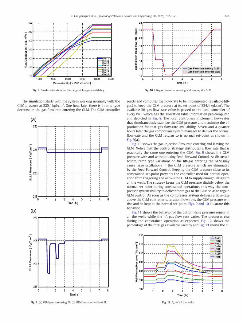
Fig. 8. Gas-lift allocation for the range of lift-gas availability. Fig. 10. Lift-gas flow-rate entering and leaving the GLM.

165E. Camponogara et al. / Journal of Petroleum Science and Engineering 70 (2010) 157–167

The simulation starts with the system working normally with theGLM pressure at 225.4 kgf/cm2. One hour later there is a ramp typedecrease in the gas flow-rate entering the GLM. The GLM controller

Fig. 9. (a) GLM pressure using FF. (b) GLM pressure without FF.

reacts and computes the flow-rate to be implemented (available lift-gas) to keep the GLM pressure at its set-point of 224.4 kgf/cm2. Theavailable lift-gas flow-rate value is passed to the local controller ofevery well which has the allocation table information pre-computedand depicted in Fig. 8. The local controllers implement flow-ratesthat simultaneously stabilize the GLM pressure and maximize the oilproduction for that gas flow-rate availability. Seven and a quarterhours later the gas compressor system manages to deliver the normalflow-rate and the GLM returns to is normal set-point as shown inFig. 9(a).

Fig. 10 shows the gas-injection flow-rate entering and leaving theGLM. Notice that the control strategy distributes a flow rate that ispractically the same one entering the GLM. Fig. 9 shows the GLMpressure with and without using Feed-Forward Control. As discussedbefore, ramp type variations on the lift-gas entering the GLM maycause large oscillations in the GLM pressure which are eliminatedby the Feed-Forward Control. Keeping the GLM pressure close to itsconstrained set-point prevents the controller used for normal oper-ation from triggering and allows the GLM to supply enough lift-gas toall the wells. The strategy keeps the GLM pressure slightly below thenormal set-point during constrained operations, this way the com-pressor system will try to deliver more gas to the GLM so as to regainGLM control. As soon as the compressor system delivers a flow-rateabove the GLM controller saturation flow-rate, the GLM pressure willrise and be kept at the normal set-point. Figs. 9 and 10 illustrate thisbehavior.

Fig. 11 shows the behavior of the bottom-hole pressure sensor ofall the wells while the lift-gas flow-rate varies. The pressures riseduring the constrained operation as expected. Fig. 12 shows thepercentage of the total gas available used by and Fig. 13 shows the oil

Fig. 11. Pwf of all the wells.

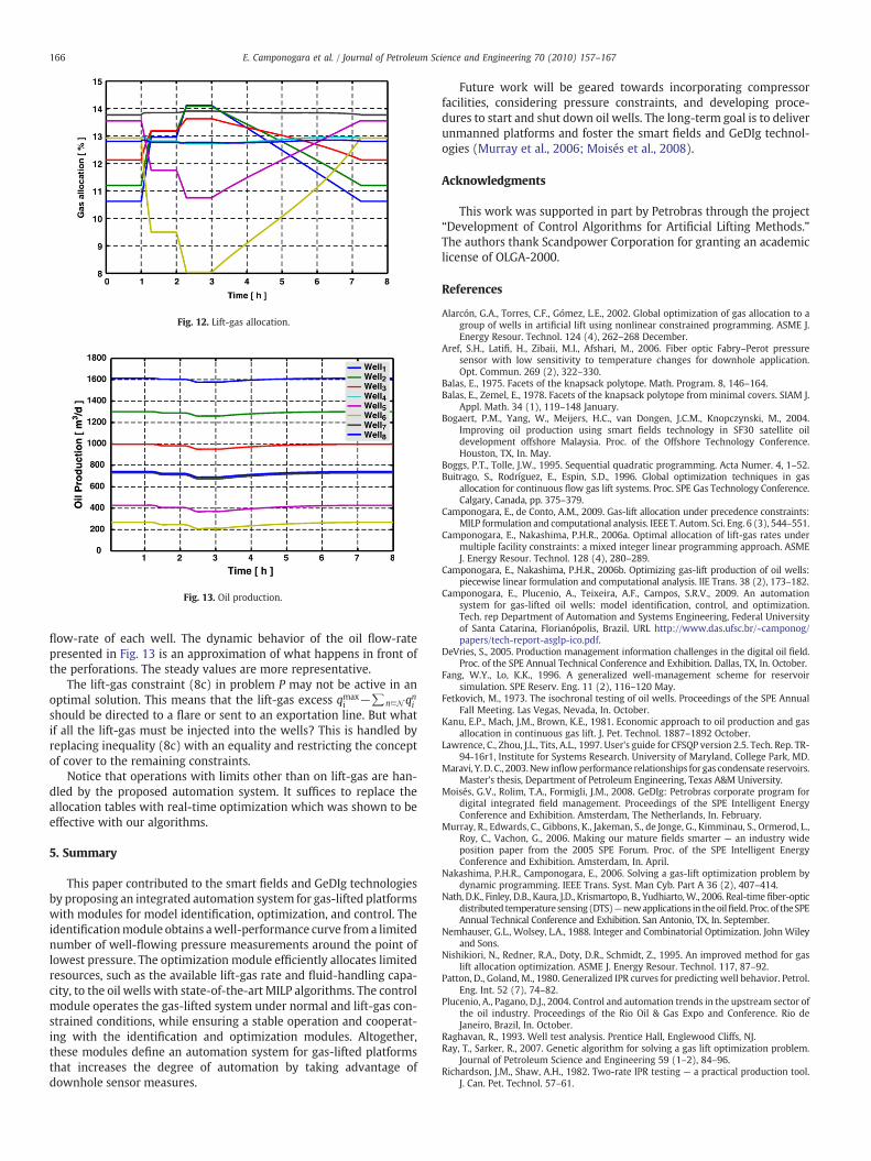
Fig. 12. Lift-gas allocation.

Fig. 13. Oil production.

166 E. Camponogara et al. / Journal of Petroleum Science and Engineering 70 (2010) 157–167

flow-rate of each well. The dynamic behavior of the oil flow-ratepresented in Fig. 13 is an approximation of what happens in front ofthe perforations. The steady values are more representative.

The lift-gas constraint (8c) in problem P may not be active in anoptimal solution. This means that the lift-gas excess qmax

i −∑n∈N qnishould be directed to a flare or sent to an exportation line. But whatif all the lift-gas must be injected into the wells? This is handled byreplacing inequality (8c) with an equality and restricting the conceptof cover to the remaining constraints.

Notice that operations with limits other than on lift-gas are han-dled by the proposed automation system. It suffices to replace theallocation tables with real-time optimization which was shown to beeffective with our algorithms.

5. Summary

This paper contributed to the smart fields and GeDIg technologiesby proposing an integrated automation system for gas-lifted platformswith modules for model identification, optimization, and control. Theidentificationmodule obtains awell-performance curve froma limitednumber of well-flowing pressure measurements around the point oflowest pressure. The optimization module efficiently allocates limitedresources, such as the available lift-gas rate and fluid-handling capa-city, to the oil wells with state-of-the-art MILP algorithms. The controlmodule operates the gas-lifted system under normal and lift-gas con-strained conditions, while ensuring a stable operation and cooperat-ing with the identification and optimization modules. Altogether,these modules define an automation system for gas-lifted platformsthat increases the degree of automation by taking advantage ofdownhole sensor measures.

Future work will be geared towards incorporating compressorfacilities, considering pressure constraints, and developing proce-dures to start and shut down oil wells. The long-term goal is to deliverunmanned platforms and foster the smart fields and GeDIg technol-ogies (Murray et al., 2006; Moisés et al., 2008).

Acknowledgments

This work was supported in part by Petrobras through the project“Development of Control Algorithms for Artificial Lifting Methods.”The authors thank Scandpower Corporation for granting an academiclicense of OLGA-2000.

References

Alarcón, G.A., Torres, C.F., Gómez, L.E., 2002. Global optimization of gas allocation to agroup of wells in artificial lift using nonlinear constrained programming. ASME J.Energy Resour. Technol. 124 (4), 262–268 December.

Aref, S.H., Latifi, H., Zibaii, M.I., Afshari, M., 2006. Fiber optic Fabry–Perot pressuresensor with low sensitivity to temperature changes for downhole application.Opt. Commun. 269 (2), 322–330.

Balas, E., 1975. Facets of the knapsack polytope. Math. Program. 8, 146–164.Balas, E., Zemel, E., 1978. Facets of the knapsack polytope from minimal covers. SIAM J.

Appl. Math. 34 (1), 119–148 January.Bogaert, P.M., Yang, W., Meijers, H.C., van Dongen, J.C.M., Knopczynski, M., 2004.

Improving oil production using smart fields technology in SF30 satellite oildevelopment offshore Malaysia. Proc. of the Offshore Technology Conference.Houston, TX, In. May.

Boggs, P.T., Tolle, J.W., 1995. Sequential quadratic programming. Acta Numer. 4, 1–52.Buitrago, S., Rodríguez, E., Espin, S.D., 1996. Global optimization techniques in gas

allocation for continuous flow gas lift systems. Proc. SPE Gas Technology Conference.Calgary, Canada, pp. 375–379.

Camponogara, E., de Conto, A.M., 2009. Gas-lift allocation under precedence constraints:MILP formulation and computational analysis. IEEE T. Autom. Sci. Eng. 6 (3), 544–551.

Camponogara, E., Nakashima, P.H.R., 2006a. Optimal allocation of lift-gas rates undermultiple facility constraints: a mixed integer linear programming approach. ASMEJ. Energy Resour. Technol. 128 (4), 280–289.

Camponogara, E., Nakashima, P.H.R., 2006b. Optimizing gas-lift production of oil wells:piecewise linear formulation and computational analysis. IIE Trans. 38 (2), 173–182.

Camponogara, E., Plucenio, A., Teixeira, A.F., Campos, S.R.V., 2009. An automationsystem for gas-lifted oil wells: model identification, control, and optimization.Tech. rep Department of Automation and Systems Engineering, Federal Universityof Santa Catarina, Florianópolis, Brazil. URL http://www.das.ufsc.br/~camponog/papers/tech-report-asglp-ico.pdf.

DeVries, S., 2005. Production management information challenges in the digital oil field.Proc. of the SPE Annual Technical Conference and Exhibition. Dallas, TX, In. October.

Fang, W.Y., Lo, K.K., 1996. A generalized well-management scheme for reservoirsimulation. SPE Reserv. Eng. 11 (2), 116–120 May.

Fetkovich, M., 1973. The isochronal testing of oil wells. Proceedings of the SPE AnnualFall Meeting. Las Vegas, Nevada, In. October.

Kanu, E.P., Mach, J.M., Brown, K.E., 1981. Economic approach to oil production and gasallocation in continuous gas lift. J. Pet. Technol. 1887–1892 October.

Lawrence, C., Zhou, J.L., Tits, A.L., 1997. User's guide for CFSQP version 2.5. Tech. Rep. TR-94-16r1, Institute for Systems Research. University of Maryland, College Park, MD.

Maravi, Y.D. C., 2003.New inflowperformance relationships for gas condensate reservoirs.Master's thesis, Department of Petroleum Engineering, Texas A&M University.

Moisés, G.V., Rolim, T.A., Formigli, J.M., 2008. GeDIg: Petrobras corporate program fordigital integrated field management. Proceedings of the SPE Intelligent EnergyConference and Exhibition. Amsterdam, The Netherlands, In. February.

Murray, R., Edwards, C., Gibbons, K., Jakeman, S., de Jonge, G., Kimminau, S., Ormerod, L.,Roy, C., Vachon, G., 2006. Making our mature fields smarter — an industry wideposition paper from the 2005 SPE Forum. Proc. of the SPE Intelligent EnergyConference and Exhibition. Amsterdam, In. April.

Nakashima, P.H.R., Camponogara, E., 2006. Solving a gas-lift optimization problem bydynamic programming. IEEE Trans. Syst. Man Cyb. Part A 36 (2), 407–414.

Nath, D.K., Finley, D.B., Kaura, J.D., Krismartopo, B., Yudhiarto,W., 2006. Real-time fiber-opticdistributed temperaturesensing(DTS)—newapplications in theoilfield. Proc. of theSPEAnnual Technical Conference and Exhibition. San Antonio, TX, In. September.

Nemhauser, G.L., Wolsey, L.A., 1988. Integer and Combinatorial Optimization. John Wileyand Sons.

Nishikiori, N., Redner, R.A., Doty, D.R., Schmidt, Z., 1995. An improved method for gaslift allocation optimization. ASME J. Energy Resour. Technol. 117, 87–92.

Patton, D., Goland, M., 1980. Generalized IPR curves for predicting well behavior. Petrol.Eng. Int. 52 (7), 74–82.

Plucenio, A., Pagano, D.J., 2004. Control and automation trends in the upstream sector ofthe oil industry. Proceedings of the Rio Oil & Gas Expo and Conference. Rio deJaneiro, Brazil, In. October.

Raghavan, R., 1993. Well test analysis. Prentice Hall, Englewood Cliffs, NJ.Ray, T., Sarker, R., 2007. Genetic algorithm for solving a gas lift optimization problem.

Journal of Petroleum Science and Engineering 59 (1–2), 84–96.Richardson, J.M., Shaw, A.H., 1982. Two-rate IPR testing — a practical production tool.

J. Can. Pet. Technol. 57–61.

167E. Camponogara et al. / Journal of Petroleum Science and Engineering 70 (2010) 157–167

Sherali, H.D., 2001. On mixed-integer zero-one representations for separable lower-semicontinuous piecewise-linear functions. Oper. Res. Lett. 28, 155–160.

Vogel, J.V., 1968. Inflow performance relationships for solution-gas drive wells. J. Pet.Technol. 83–92 January.

Wang, P., Litvak, M., Aziz, K., 2002. Optimization of production operations in petroleumfields. Proc. 17th World Petroleum Congress. Rio de Janeiro.

Wiggins, M.L., Russel, J.E., Jennings, J., 1996. Analytical development of vogel-typeinflow performance relationships. SPE J. 355–362 December.

Williams, C., Webb, T., 2007. Shell strives to make smart fields smarter. Society ofPetroleum Engineers. July.

Yeten, B., Jalali, Y., 2001. Effectiveness of intelligent completions in a multiwelldevelopment context. Proc. of the SPE Middle East Oil Show. March.

Yeten, B., Brouwer, D.R., Durlofsky, L.J., Aziz, K., 2004. Decision analysis underuncertainty for smart well deployment. J. Pet. Sci. & Eng. 43 (3–4), 183–199.