AN AUTOMATED DENTAL CARIES DETECTION AND ...

Virginia Commonwealth University Virginia Commonwealth University

VCU Scholars Compass VCU Scholars Compass

Theses and Dissertations Graduate School

2014

AN AUTOMATED DENTAL CARIES DETECTION AND SCORING AN AUTOMATED DENTAL CARIES DETECTION AND SCORING

SYSTEM FOR OPTIC IMAGES OF TOOTH OCCLUSAL SURFACE SYSTEM FOR OPTIC IMAGES OF TOOTH OCCLUSAL SURFACE

Leila Ghaedi Virginia Commonwealth University

Follow this and additional works at: https://scholarscompass.vcu.edu/etd

Part of the Dentistry Commons

© The Author

Downloaded from Downloaded from https://scholarscompass.vcu.edu/etd/3548

This Dissertation is brought to you for free and open access by the Graduate School at VCU Scholars Compass. It has been accepted for inclusion in Theses and Dissertations by an authorized administrator of VCU Scholars Compass. For more information, please contact [email protected].

AN AUTOMATED DENTAL CARIES DETECTION AND SCORING SYSTEM

FOR OPTIC IMAGES OF TOOTH OCCLUSAL SURFACE

A dissertation submitted in partial fulfillment of the requirements for the

degree of Doctor of Philosophy at Virginia Commonwealth University.

by

LEILA GHAEDI

Advisor: ROSALYN HARGRAVES HOBSON

Associate Professor, Department of Electrical and Computer

Engineering

Virginia Commonwealth University

Richmond, VA

June, 2014

ii

ACKNOWLEDGMENT

First and foremost, I would like to express my most sincere gratitude to my advisor; Dr. Rosalyn

Hobson Hargraves for the help, encouragement and support she provided me during this

research. I would like to thank Dr. Kayvan Najarian and Dr. Riki Gottlieb for their guidance and

encouragement through my entire research and for their invaluable insights and comments. I am

grateful to my committee members, Dr. Alen Docef and Dr. Yuichi Motai for their feedback on

my work. I would like to thank my colleagues at the VCU Biomedical Signal Image Processing

Laboratory for making this journey a lot more fun. I would like to thank my best friend and

spouse, Omid Akbarzadeh for his love and support and my wonderful parents, Zahra Roshan and

Ali Ghaedi for their unconditional love and support. Their support and guidance has given me an

extraordinary platform to pursue and achieve my dreams.

iii

Contents

Acknowledgement ii

Abstract x

Novelty and Contribution xi

1 Introduction 1

1.1 Aim 1

1.2 Motivation 2

1.2.1 Dental Caries Detection Impact 2

1.2.2 Objectives 3

1.3 Overview of Dissertation 4

2 Background 6

2.1 Introduction 6

2.2 Caries Detection and ICDAS guideline 7

2.3 Image Segmentation Methods 11

2.3.1 Threshold-Based Methods 11

2.3.2 Region Growing Methods 11

2.3.3 Active Contour Models (Snakes) 12

2.3.4 Color Image Segmentation 13

2.3.4.1 Color Space Presentation 14

2.4 Classification Methods 15

2.4.1 Support Vector Machine (SVM) 15

2.4.2 C4.5 Decision Tree 16

iv

2.4.3 Random Forest Tree 16

2.4.4 Neural Network Classifier 17

2.5 Feature Extraction 18

2.6 Feature Selection Methods 18

2.7 Overview of the Method 19

3 Tooth Surface Segmentation 21

3.1 Introduction 21

3.2 Pre-Processing 22

3.3 Initial Single Seed Selection 23

3.3.1 Modified Circular Hough Transform 24

3.4 Color Image Seeded Region Growing 27

3.4.1 Measure of Similarity for HSV Space 28

3.5 Active Contour Model 28

4 Irregular Region Segmentation 30

4.1 Introduction 30

4.2 Texture Analysis 30

5 Feature Selection and Classification 33

5.1 Feature Extraction 33

5.2 Feature Selection and Classification 34

6 Description of Data Set 40

6.1 Introduction 40

6.2 In-Vitro Data Set 40

v

6.2.1 First In-Vitro Data Set 40

6.2.2 Second In-Vitro Data Set 41

6.3 In-Vivo Data Set 42

7 Results and Discussion 45

7.1 Pre-Processing Results 45

7.2 Initial Seed Selection Results 48

7.3 Region Growing and Active Contour Model Results 52

7.4 Irregular Region Segmentation Results 59

7.5 Feature Selection and Classification Results 62

7.6 Alternative System 66

8 Summary and Future Work 68

8.1 Summary 68

8.2 Future Work 69

REFERENCES 70

APPENDICES 77

vi

List of Figures

2.1 Schematic section tooth 10

2.2 HSV color space 14

2.3 Diagram of the system components 20

3.1 Calculating the line segment perpendicular to the edge- limited by minimum and

maximum possible radius- for any detected edge, any pixel with the coordinates of red line in

accumulation array will get a value 25

3.2 4-Neighbourhood 27

3.3 An Active Contour Model, over a series of iterations, the active contour moves into

alignment with the nearest salient feature, in this case an edge 29

4.1 Segmentation workflow 32

5.1 Re-categorization map of seven ICDAS scores into three classes 35

5.2 The histogram of ICDAS and reduced ICDAS3 for 94 images 35

5.3 Re-categorization map for Ekstrand histological scores: five histological scores mapping

into three classes 37

5.4 Filter based feature reduction and super classifier diagram 39

6.1 One example of First In-Vivo Data Set 41

6.2 One example of Second In-Vivo Data Set 42

6.3 KODAK A1500 Intraoral Camera 42

6.4 Example of three different views of one tooth of In-Vivo Data Set 44

7.1 Pre-processing- Tooth #24 - First In-Vitro Data Set 46

7.2 Pre-processing- Tooth #14- Second In-Vitro Data Set 47

vii

7.3 Pre-processing- Tooth #23 - In-Vivo Data Set 48

7.4 Accumulation array of tooth #4 of Second In-Vitro Data Set 49

7.5 Output of CHT (multiple circle centers and radii) for the same image as figure 7.450

7.6 Final seed for the same image as figure 7.4 50

7.7 Accumulation array of tooth #12 of In-Vivo Data Set 51

7.8 Output of CHT (multiple circle centers and radii) for the same image as figure 7.751

7.9 Final seed for the same image as figure 7.7 52

7.10 Image #2 -In-Vitro Data Set; From up left to down right; 1: Original image, 2: Region

growing output, 3: Active contour model Output, 4: Active contour model output black and

white mask 53

7.11 Image #12 -In-Vitro Data Set; From up left to down right; 1: Original image, 2: Region

growing output, 3: Active contour model Output, 4: Active contour model output black and

white mask 54

7.12 Image #6 -In-Vitro Data Set (The same tooth with image # 12 in Figure 7.11); From up

left to down right; 1: Original image, 2: Region growing output, 3: Active contour model Output,

4: Active contour model output black and white mask 55

7.13 Image #39 -In-Vitro Data Set; From up left to down right; 1: Original image, 2: Region

growing output, 3: Active contour model Output, 4: Active contour model output black and

white mask 56

7.14 Image #42 -In-Vitro Data Set (The same tooth with image # 39 in Figure 7.13); From up

left to down right; 1: Original image, 2: Region growing output, 3: Active contour model output,

4: Active contour model output black and white mask 57

7.15 Tooth segmentation results for 88 in-vitro images- S2 refers to region growing step

output and S3 refers to Active contour model output 58

7.16 Tooth segmentation results for 50 in-vivo images- S2 refers to region growing step

output and S3 refers to Active contour model output 59

7.17 Image #23 - First In-Vitro Data Set – Irregular regions 60

7.18 Image #2 - Second In-Vitro Data Set – Irregular regions 61

7.19 Image #24 - In-Vivo Data Set – Irregular regions 62

viii

7.20 Reduced feature pool (32 features) vs 3 ICDAS classes; dark blue class (0), red class

(1,2) and cyan class(3-6) 63

7.21 Final selected features (12 features) box plot grouped by 3 ICDAS classes 64

7.22 Diagram of the alternative system components 67

ix

List of Tables

2.1 ICDAS scores’ description 10

5.1 Feature Extraction 34

7.1 Final selected features description (12 features) 65

7.2 Confusion Matrix; this table shows the confusion matrix for the designed system,

comparing it to the ICDAS scores. The designed system’s scores has been generated by the

system and where ICDAS experts’ scores are the scores that ICDAS experts assigned to each

tooth after examining the extracted tooth as well as looking at the images of occlusal surface

65

ABSTRACT

AN AUTOMATED DENTAL CARIES DETECTION AND SCORING SYSTEM

FOR OPTIC IMAGES OF TOOTH OCCLUSAL SURFACE

by Leila Ghaedi, Ph.D.

A dissertation submitted in partial fulfillment of the requirements for the

degree of Doctor of Philosophy at Virginia Commonwealth University

Virginia Commonwealth University, 2014

Advisor: Rosalyn Hobson Hargraves, Associate Professor, Department of Electrical and

Computer Engineering

Dental caries are one of the most prevalent chronic diseases. Worldwide 60 to 90 percent of

school children and nearly 100 percent of adults experienced dental caries. The management of

dental caries demands detection of carious lesions at early stages. The research of designing

diagnostic tools in caries has been at peak for the last decade. This research aims to design an

automated system to detect and score dental caries according to the International Caries

Detection and Assessment System (ICDAS) guidelines using the optical images of the occlusal

tooth surface. There have been numerous works that address the problem of caries detection by

using new imaging technologies or advanced measurements. However, no such study has been

done to detect and score caries with the use of optical images of the tooth surface. The aim of

this dissertation is to develop image processing and machine learning algorithms to address the

problem of detection and scoring the caries by the use of optical image of the tooth surface.

xi

Novelty and Contribution

Dental caries are one of the most prevalent chronic diseases in the world. According to World

Health Organization report on oral health nearly 100 percent of adults experienced dental caries.

Scientific evidences show that the early stages of caries can be arrested and possibly reversed by

noninvasive intervention such as reduction of cariogenic diet, oral hygiene improvement and

fluoride therapy in various delivery modalities. The opportunity of reversing the caries

development noninvasively introduced an everyday challenge to the dentists to determine

whether noninvasive intervention or restorative intervention is required based on severity and

activity of carious lesion; the diagnostic tools can help with decision making in this stage.

A number of existing technologies for caries diagnosis include devices based on laser

fluorescence or infrared, electrical conductance measurements, direct digital radiography, etc. are

available. These technologies have relatively high prices and also are user sensitive and require

several steps in order to perform a clinical reading correctly. The value given by these caries

detection devices is subjectively interpreted by the clinician and thus requires a trained dental

professional to make a diagnostic or treatment decision. This study uses the optical images of the

tooth surface taken by intraoral cameras, which are relatively easy to use, widely available and

inexpensive hardware imaging technique, to give a quantitative score of caries severity as well as

visual feedback. This may easily augment the decision making process of treatment provided to

patients.

The design of this diagnostic tool is very challenging due variation in image quality, presence of

natural pits and fissure areas in tooth surface and presence of several other organs and textures in

the images. Described below, the methods presented in this dissertation have several novel

components that address the above-mentioned challenges.

xii

1. A novel multi stage image segmentation algorithm is created, which incorporates shape, color

and gradient specifications of the tooth image.

The presence of normal or carious pits and fissure areas in the tooth surface especially when the

change of color occurs near the tooth boundary fails any conventional image segmentation

method to segment the tooth surface properly. The proposed segmentation method uses the

particular shape of the tooth to find a unique seed point; then uses a top down approach to find

out the tooth boundary based on color information and finally refines the output of previous step

to the actual tooth surface using a bottom up approach which is applied to the gradient of gray

scale image.

2. A modified version of Circular Hough Transform (CHT) is created which uses the tooth shape

to find the initial seed point.

Original CHT finds too many false circles in the images. The proposed method applies a series

of modification to CHT to address the false circles detection. The calculation of accumulation

array is limited to a set of minimum and maximum possible radius. The limits defined based on

the application to reduce the computational cost and avoid finding false circles. A level of

thresholding applied to the gradient values and another threshold applied to the accumulation

array values to reduce the false detected circles.

3. A novel algorithm is proposed to define presence of irregularities in the tooth occlusal

surface; irregular regions are the region of interest for dentists while they examine the tooth.

While the irregular regions are defined qualitatively by the dentists based on different color,

translucency and porosity; the proposed method utilizes texture analysis and morphological

operators to map the irregular regions.

xiii

4. The novel feature extraction algorithm was developed to incorporate the texture and

morphological information as well as color and intensity levels in the feature space.

The proposed method utilizes a novel approach by calculation of the color and intensity based

features on two different masks (irregular regions and tooth surface except irregular regions).

Since the irregular region mask encompasses the texture and morphological information, by

separate calculation of color and intensity levels for these regions; the final feature space not

only has the color and intensity level information but also the texture information.

1

Chapter 1

Introduction

1.1 Aim

The aim of this dissertation is to design an automated system to detect and score dental caries

according to the International Caries Detection and Assessment System (ICDAS) guidelines

using the optical images of the occlusal tooth surface. The imaging technologies and advanced

measurements for caries detection have been an active area of research for the last decade. The

final goal of early caries detection tools is to provide an adjacent to clinical decision making and

support preventive treatment planning in conjunction with caries risk assessment which finally

reduce the risk of premature restoration intervention. However, no such study has been done to

detect and score caries with the use of optical images. All the available imaging technologies for

caries detection have relatively high prices. Any of the current technologies do not consider

information present in the optical images. This study has been designed to incorporate digital

images acquired from off-the-shelf commercially available intraoral cameras which are

inexpensive in comparison to other dental imaging modalities. By applying image processing

techniques, several features extracted from the image of the tooth surface and those features will

provide the measures for scoring the tooth according to ICDAS guidelines. These features reveal

the spatial information along with texture parameters of the whole tooth area as well as the

detected irregular regions.

2

1.2 Motivation

1.2.1 Dental Caries Detection Impact

Dental caries are one of the most prevalent chronic diseases in the world. According to World

Health Organization report on oral health at April 2012, worldwide 60 to 90 percent of school

children and nearly 100 percent of adults experienced dental caries [1]. A significant general

reduction in caries lesions has been noted in the United States in the last several decades with the

increased availability of fluoride in public water supply, tooth paste and mouth rinse [2]. The

widespread use and availability of fluoride has changed the behavior of carious lesions

dramatically. The resulted slower progression of carious lesions has afforded the dental

profession the opportunity to diagnosis and manage caries at an early stage [3]. Scientific

evidences show that the early stages of caries can be arrested and possibly reversed by

noninvasive intervention such as reduction of cariogenic diet, oral hygiene improvement and

fluoride therapy in various delivery modalities. The opportunity of reversing the caries

development noninvasively introduced an everyday challenge to the dentists to determine

whether noninvasive intervention or restorative intervention is required based on severity and

activity of carious lesion; the diagnostic tools can help with decision making in this stage [3].

Clinical standards for diagnosing caries include visual examination, tactile sensation, aided by

radiography combined with patient's individual caries risk levels. Visual examination assesses

color, translucency and porosity while tactile examination evaluates hardness and porosity using

explorers. When using traditional examination for caries detection; the end result is low

sensitivity and high specificity, meaning a large number of lesions may be missed. In addition,

using traditional diagnostic methods for diagnosing pit and fissure caries on occlusal surfaces

have a high false positive and false negative rate [4-5]. On the other hand, the greatest reduction

3

in caries has been noted in smooth tooth surfaces and this type of interproximal lesion can be

more easily identified by radiographic techniques [6]. Occlusal lesions have become the largest

proportion of the total caries burden [4]. In addition, the current diagnostic methods have a high

false positive and false negative rate when diagnosing pit and fissure caries on occlusal surfaces

[4-5]. Existing technologies for caries diagnosis include devices based on laser fluorescence (LF)

such as LF device, LF pen, LF camera, or infrared (IR) laser fluorescence, referred to as

quantitative laser or light fluorescence (QLF). Electrical conductance measurements (ECM),

direct digital radiography, Digital Imaging Fiber-Optic Trans-Illumination (DIFOTI) and simple

Fiber Optic Trans-Illumination (FOTI), LED-based caries detector and less popular fluorescence

spectrophotometer, MicroCT and heat induced detection technique [3, 7-12]. Data shows varying

degrees of sensitivity and specificity for In-Vitro and In-Vivo studies [3, 8- 9, 13-15]. These

technologies have relatively high prices and also are user sensitive and require several steps in

order to perform a clinical reading correctly. The value given by these caries detection devices is

subjectively interpreted by the clinician and thus requires a trained dental professional to make a

diagnostic or treatment decision.

Accurate detection of dental caries, in particular at the early stages, can greatly improve the

quality of dental care. The method uses the optical images of the tooth surface taken by intraoral

cameras, which are relatively easy to use, widely available and inexpensive hardware imaging

technique. This may easily augment the decision making process of treatment provided to

patients and their overall impression of the quality of dental care they are receiving.

1.2.2 Objectives

The objective of this thesis dissertation is to design an automated system to detect and score

dental caries. The input of the system is the optical image of occlusal tooth surface which has

4

been taken with the intraoral camera and the output of the system is an ICDAS score which

quantify the presence and severity of caries on that tooth surface. Solving this particular problem

needs several stages. The first stage of this work is to design an image segmentation method to

segment the image into background, regular tooth surface and region of interest for the dentists,

which are called; irregular regions. The second stage is extracting features from the segmented

areas. The last stage is a classification problem which assigns a score to each image with regard

to the severity of the caries on the tooth surface.

The objectives of this dissertation are summarized as follows:

� Create a novel segmentation method, to effectively segment the tooth surface images

(both in-vitro and in-vitro images) into background, regular tooth surface and irregular

regions according to the guidelines for clinical caries detection.

� Design a feature extraction algorithm that allows for the accurate classification of the

dental carries. The extraction of features in medical image applications is a very crucial task.

The method utilizes the extracted features and selects only the predominant features through

a multi-stage feature selection process in order to automatically score the caries.

� Create a novel classification technique classifies the features extracted from tooth images into

the clinical scores. For computing the classification model, an ensemble classifier has been

developed which essentially encompasses four different classification methods.

1.3 Overview of Dissertation

This thesis dissertation is organized as follows.

Chapter 2 provides an overview for the background of the problem. First, International Caries

Detection and Assessment System (ICDAS) guidelines are introduced. Then, image

5

segmentation methods are presented followed by an overview of feature selection and

classification methods.

Chapter 3 describes the multi staged segmentation method which results the segmentation of

tooth boundary from the complicated background.

Chapter 4 presents the application of texture analysis to segment the irregular regions inside the

tooth.

Chapter 5 presents feature extraction, feature selection and feature classification methods which

used to classify each tooth to different caries severity classes.

Chapter 6 describes specification of the data sets.

Chapter 7 provides the results and the discussion to assess the performance of the methods.

Chapter 8 describes a summary of the work and the future work for this study.

6

Chapter 2

Background

2.1 Introduction

While carries detection is paramount in the field of cardiology, most in practice methods utilize

traditional visual inspection. No similar study has been done to provide a decision support

system in the field of cariology with the use of optical images. Moreover none of the current

caries detection technologies provide a quantitative feedback for caries management along with

visual feedback. Some existing technologies for caries diagnosis are using other types of images

such as radiographic images, laser fluorescence images, Fiber-Optic Trans-Illumination images

and simple Fiber Optic Trans-Illumination images. Due to different nature of these types of

images and optical images of the tooth surface which is the subject of this study, and also

different appearance of caries lesions, the image processing methods used in current technologies

are not applicable to our problem. However none of the current caries detection devices provided

a dental decision support system with the application of machine learning tools. These devices

are subjectively interpreted by the clinician and thus require a trained dental professional. The

other types of caries diagnosis technologies, such as Electrical conductance measurements

(ECM) do not provide any visual feedback [3, 7-12].

7

With the lack of background in the field of study in dental applications, this study rely on the

other areas of medical decision support systems’ background, especially those with medical

image processing components.

This chapter provides an overview of the ICDAS standard as well as image segmentation,

classification and feature extraction algorithms which have been used in the medical decision

support systems.

2.2 Caries Detection and ICDAS Guideline

Clinical standards for diagnosing carious lesions of teeth include visual inspection of tooth

surface for color and translucency evaluation, analysis of radiographic images, evaluation of

dental surface porosity or hardness; visually or using tactile sense combined with patient's

individual caries risk levels [7,16]. As the understanding of dental caries progressed, the clinical

criteria systems remained focused on assessment the disease process at only one stage, the so

called ‘decayed’ status. In April and August 2002, a group of caries researchers, epidemiologists,

and restorative dentists, met to integrate the different definitions. The group selected a

foundation for a new system and proposed a new system which was named the International

Caries Detection and Assessment System (ICDAS). A study in 2004, reviewed 29 caries

detection criteria systems concluded that the majority of the caries detection systems were

ambiguous and did not measure the disease process at its different stages [5]. In 2005, the

Rationale and Evidence for the International Caries Detection and Assessment System was

presented, followed by the publication of the modified International Caries Detection and

Assessment System Criteria Manual [17]. The ICDAS integrated several criteria systems into

one standard system for caries detection and assessment [17]. The ICDAS measures the surface

changes and potential histological depth of carious lesions by relying on surface characteristics.

8

The ICDAS evaluation of pit and fissure caries is based on biological processes of

demineralization followed by re-mineralization manifested clinically as changes in color or

cavitation. According to ICDAS the dental examiners evaluate the tooth surface and classify the

carious status of each tooth surface using a seven-point ordinal scale ranging from sound to

extensive cavitation. The classification of the carious status based upon ICDAS is as follows.

Sound Tooth Surface (Score 0): There should be no evidence of caries, either no or

questionable change in enamel translucency after prolonged air drying for 5 seconds. First

visual change in enamel (Score 1): When seen wet there is no evidence of any change in color

attributable to carious activity, but after prolonged air drying for 5 seconds carious opacity or

discoloration (white or brown lesion) is visible that is not consistent with the clinical appearance

of sound enamel. Distinct visual change in enamel (Score 2): The tooth must be viewed wet.

There is a carious opacity, white spot lesion and/or brown carious discoloration which are wider

than the natural fissure that is not consistent with the clinical appearance of sound enamel; the

lesion must still be visible when dry. Localized enamel breakdown because of caries with no

visible dentin or underlying shadow (Score 3): The tooth viewed wet may have a clear carious

opacity, white spot lesion and/or brown carious discoloration which is wider than the natural

fissure that is not consistent with the clinical appearance of sound enamel. After drying for

approximately 5 seconds there is carious loss of tooth structure at the entrance to, or within, the

pit or fissure area. Underlying dark shadow from dentin with or without localized enamel

breakdown (Score 4): This lesion appears as a shadow of discolored dentin visible through an

apparently intact enamel surface which may or may not show signs of localized breakdown, loss

of continuity of the surface that is not showing the dentin. The shadow appearance is often seen

more easily when the tooth is wet. The darkened area is an intrinsic shadow which may appear as

9

grey, blue or brown in color. The shadow must clearly represent caries that started on the tooth

surface being evaluated. Distinct cavity with visible dentin (Score 5): Cavitation in opaque or

discolored enamel exposing the dentin beneath. The tooth viewed wet may have darkening of the

dentin visible through the enamel. Once dried for 5 seconds there is visual evidence of loss of

tooth structure at the entrance to or within the pit or fissure frank cavitation. There is visual

evidence of demineralization such as opaque (white), brown or dark brown walls at the entrance

to or within the pit or fissure and in the examiner judgment dentin is exposed. The

WHO/CPI/PSR probe can be used to confirm the presence of a cavity apparently in dentin. This

is achieved by sliding the ball end along the suspect pit or fissure and a dentin cavity is detected

if the ball enters the opening of the cavity and in the opinion of the examiner the base is in

dentin. Extensive distinct cavity with visible dentin (Score 6): Obvious loss of tooth structure,

the cavity is both deep and wide and dentin is clearly visible on the walls and at the base. An

extensive cavity involves at least half of a tooth surface or possibly reaching the pulp [17]. The

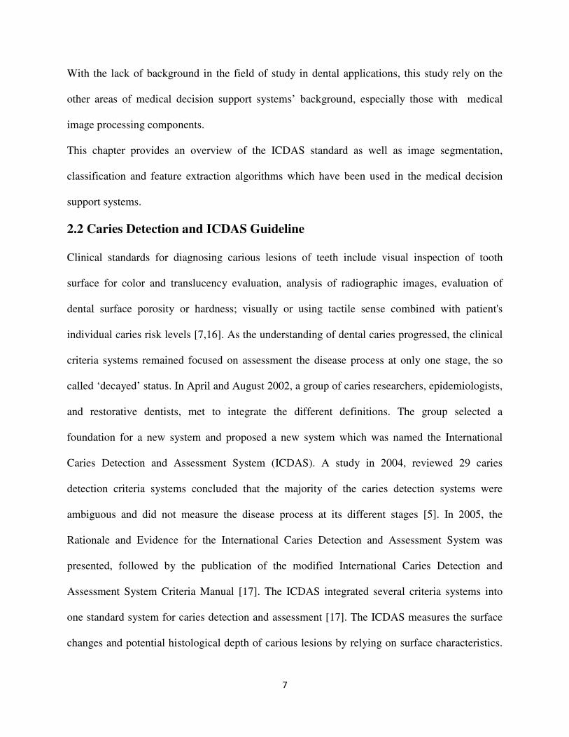
description of the scoring system has been provided in table 2.1. Figure 2.1 provides a schematic

section of the tooth structure, which illustrates dentin and enamel locations.

Often this process is not detectable using the current technology available for In-Vivo use [17].

In-Vitro studies of ICDAS validated the practicality of the system and its correlation with

histological examination of pits and fissures in occlusal surfaces of extracted teeth [18]. Studies

assessed inter- and intra-examiner reproducibility and accuracy in the detection and assessment

of occlusal caries in extracted teeth using ICDAS, using histology as 'gold standard'. ICDAS-II

presented good reproducibility and accuracy in detecting occlusal caries [19] and was able to

especially identify caries lesions in the outer half of the enamel [8]. More recently, the accuracy

of ICDAS was measured In-Vivo to compare performance of automated caries detection devices.

10

The teeth were then extracted and ICDAS was validated based on histological findings [8-20].

ICDAS demonstrated good performance in helping detect occlusal caries In-Vivo and moreover,

better accuracy was achieved in detecting early lesions [20]. A recent study assessed the

agreement among four techniques used as gold standard for the validation of methods for

occlusal caries detection and concluded that the outcome of caries diagnostic tests may be

influenced by the validation method applied [23], hence the difference in ICDAS accuracy

between studies. Based on this evidence of the validity of the ICDAS in caries diagnosis, ICDAS

scores were used in this study as the gold standard.

ICDAS Score

Description

0 Sound Tooth

1 First visual Change in Enamel

2 Distinct Visual Change in Enamel

3 Localized Enamel Breakdown

4 Underlying Dentin Shadow

5 Distinct Cavity with Visible Dentin

6 Extensive Cavity with Visible Dentin

Table 2.1: ICDAS scores’ description

Figure 2.1: Schematic section tooth [22]

11

2.3 Image Segmentation Methods

Image segmentation plays a crucial role in many medical imaging applications by automating or

facilitating the delineation of anatomical structure or other regions of interest [23]. In medical

imaging, typically the task of segmentation corresponds to different organs, biological structures

or pathologies. Segmentation methods use either discontinuity or homogeneity of gray level

values in a region to define the segments. Partitioning based approaches form the segments by

detecting isolated points, lines and edges according to abrupt changes in gray levels.

Homogeneity based algorithms include thresholding, clustering, region growing, and region

splitting and merging.

2.3.1 Threshold-Based Methods

These methods are among the simplest methods used for segmentation. Threshold based image

segmentation techniques discriminate regions on the basis of intensity value difference between

pixels. The pixels in the image are classified into two classes based on some predefined threshold

value [23-30]. Threshold for image segmentation has been calculated based on maximum

entropy, interclass variation or histogram. Threshold based segmentation does not account for

spatial characteristics of an image, making it sensitive to noise and intensity inhomogenities.

The threshold based segmentation techniques perform well for images which have only two

components; for complex images, these methods are often used as an initial step in a sequence of

image processing operations [31].

2.3.2 Region Growing Methods

The idea of region based algorithms comes from the observation that pixels inside a structure

tend to have similar intensities. Region growing techniques are used to segment regions based on

12

some similarity criteria. Each region of interest (ROI) requires its own seed initialization, after

selecting the initial seeds, algorithm searches for the neighborhood pixels which have intensities

within a predefined interval [23-24]. To eliminate the need for manual seed initialization, some

algorithms used the statistical information and a prior knowledge of the ROIs to select the seeds

semi automatically or fully automatically. The drawbacks of these methods are that they are

sensitive to the seed selection and also sensitive to the noise, sometimes the similarity criterion is

not exactly defined, also the algorithm mainly relies on the image intensity information. In

addition, these techniques are dominated by the growth of the current region. Region growing

methods are simple techniques that provide good results especially with smaller region

segmentation once all mentioned challenges are properly addressed.

2.3.3 Active Contour Models (Snakes)

Active contour models (ACMs) or snakes employ model-based methods that use a prior model to

try to find the best match for the model within the image. Active contour models are often called

snakes because they appear to slither across image edges. ACMs are one example of the general

technique of matching a deformable model to an image using energy minimization. From any

starting point, subject to certain constraints, ACM will deform into alignment with the nearest

salient feature in the image; such features correspond to local minima in the energy generated by

processing the image. ACMs provide a low-level mechanism that seeks appropriate local minima

rather than searching for a global solution. In comparison to bottom-up image processing

techniques, this technique uses a top-down approach. The ACM algorithm makes use of the

identification of local structures such as edges, points and other low-level structures in the image

that are assembled into groups to find the objects. The ACM algorithm creates a model of the

shape that uses two opposing energy terms, an internal term which works towards smoothing the

13

curve, and an external term which moves the curves towards image features, to locate the outline

of an object. ACMs are good for amorphous objects like cells, but they tend not to perform well

with objects that have a known shape. The ACM algorithm does not try to solve the entire

problem of finding salient image features; they rely on high-level mechanisms to place them

somewhere near a desired solution (a prior knowledge). For example, automatic initialization

procedures can use standard image processing techniques to locate features of interest that are

then refined using snakes [32, 33].

2.3.4 Color Image Segmentation

Color segmentation presents its own unique challenges. Color segmentation approaches are

based on monochrome segmentation approaches operating in different color spaces. There is no

uniquely superior technique, as each application presents its own specific challenges and all of

the existing color image segmentation approaches are strongly application dependent. An image

segmentation problem is basically one of psychophysical perception, and it is essential to

supplement any mathematical solutions by a priori knowledge about the image in specific

application. Most gray level image segmentation techniques could be extended to color image,

such as histogram thresholding, clustering, region growing, edge detection and fuzzy based

approaches. They can be directly applied to each component of a color space, and then the results

can be combined in some way to obtain the final segmentation result. However, one of the

problems is how to employ the color information as a whole for each pixel. When color is

projected onto three components, the color information is so scattered that the color image

becomes simply a multispectral image and the color information that human can perceive is lost.

Another problem is how to choose the color representation for segmentation, since each color

representation has its advantages and disadvantages [34]. In most of the existing color image

14

segmentation approaches, the definition of a region is based on similar color. This assumption

often makes it difficult for many algorithms to separate the objects with highlights, shadows,

shading or texture which cause inhomogeneous colors of the objects’ surface.

2.3.4.1 Color Space Presentation

Color is perceived by humans as a combination of tristimuli R (red), G (green), and B (blue)

which usually called the three primary colors. Several color representations are defined by linear

or nonlinear transformations of RGB space. Several color spaces, such as RGB, HSV and CIE

are utilized in color image segmentation, but none of them outperforms the others for all kinds of

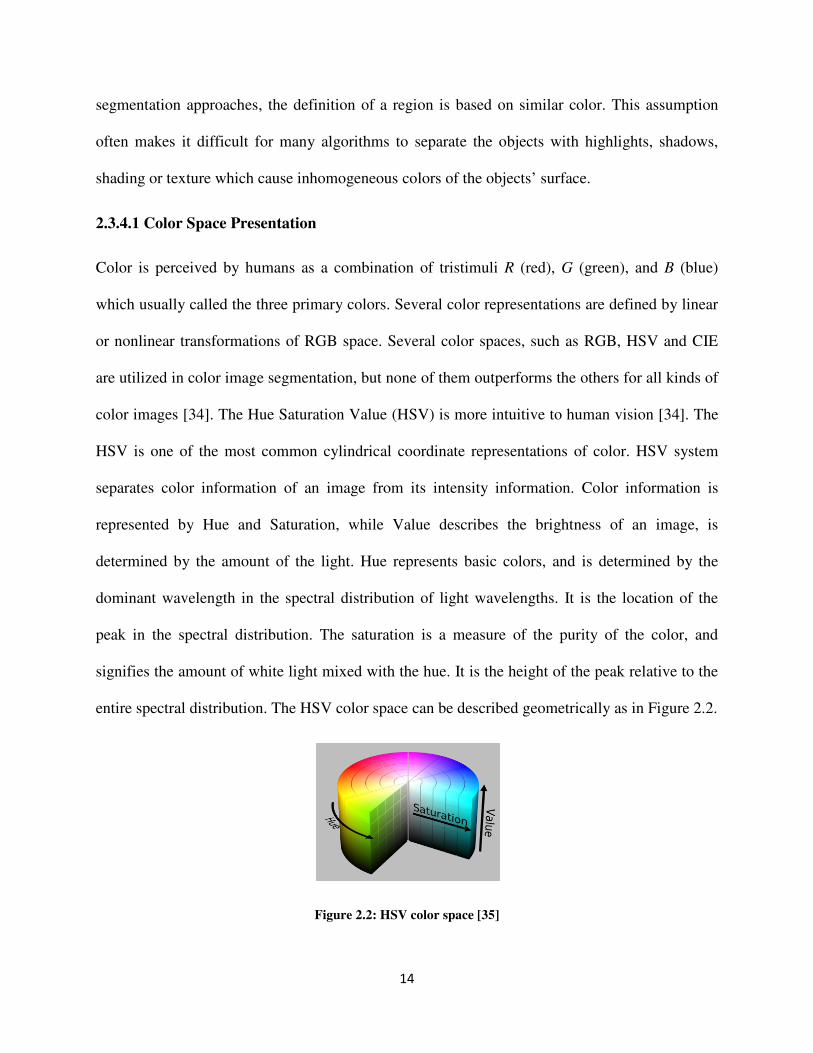
color images [34]. The Hue Saturation Value (HSV) is more intuitive to human vision [34]. The

HSV is one of the most common cylindrical coordinate representations of color. HSV system

separates color information of an image from its intensity information. Color information is

represented by Hue and Saturation, while Value describes the brightness of an image, is

determined by the amount of the light. Hue represents basic colors, and is determined by the

dominant wavelength in the spectral distribution of light wavelengths. It is the location of the

peak in the spectral distribution. The saturation is a measure of the purity of the color, and

signifies the amount of white light mixed with the hue. It is the height of the peak relative to the

entire spectral distribution. The HSV color space can be described geometrically as in Figure 2.2.

Figure 2.2: HSV color space [35]

15

2.4 Classification Methods

The task of assigning an input vector, to several classes is called a classification problem. The

input vector of N components is called a pattern and each component of the input vector is called

a feature. The task of classifying data is to decide class membership y′ of an unknown data

item x′ based on a data set � = ���, ���,… , ��, �� data items xi with known class

memberships yi. For ease of discussion, only dichotomous classification problems are

considered, where the class labels y are either 0 or 1. The xi are usually N-dimensional vectors,

the components of which are called covariates and independent variables in statistics parlance

or features by the machine learning community. In most problem domains, there is no functional

relationship y=f(x) between y and x. In this case, the relationship between x and y has to be

described more generally by a probability distribution P(x,y); one then assumes that the data

set D contains independent samples from P. From statistical decision theory, it is well known

that the optimal class membership decision is to choose the class label y that maximizes the

posterior distribution P(y|x). In this dissertation the features are statistical measures of the tooth

image and the classes are caries scores according to ICDAS. The design of this study is based on

supervised learning paradigm. There are several machine learning algorithms to choose from,

where the choice simply depends on the type of dataset and its complexity. Four popular

classification methods which has been used in medical decision support applications introduces

in this session [36].

2.4.1 Support Vector Machine (SVM)

Support vector machines are algorithmic implementations of ideas from statistical learning

theory. Statistical learning theory solves the problem of building consistent estimators from data,

meaning by having only characteristics of the model, and performance on a training set, how the

16

performance of a model on an unknown data set can be estimated. SVMs build optimal

separating boundaries between data sets by solving a constrained quadratic optimization

problem. By using different kernel functions, varying degrees of nonlinearity and flexibility can

be included in the model. Because they can be derived from advanced statistical ideas, and

bounds on the generalization error can be calculated for them, support vector machines have

received considerable research interest over the past years. The disadvantage of support vector

machines is that the classification result is purely dichotomous, and no probability of class

membership is given.

2.4.2 C4.5 Decision Tree

The C4.5 algorithm builds decision trees from a set of training data in the, using the concept

of information entropy. The input vector of N components is called a pattern and each

component of the input vector is called a feature. The task of classifying data is to decide class

membership y′ of an unknown data item x

′ based on a training data set D=(x1,y1),…,(xn,yn) of data

items xi with known class memberships yi. At each node of the tree, C4.5 chooses the feature of

the data that most effectively splits its set of samples into subsets enriched in one class or the

other. The splitting criterion is the normalized information gain (difference in entropy). The

feature with the highest normalized information gain is chosen to make the decision.

2.4.3 Random Forest Tree

Random forests are a combination of tree classifiers such that each tree depends on the values of

a random vector sampled independently and with the same distribution for all trees in the forest.

Random forest uses multiple trees or a forest to develop decisions and classifications. Random

forest can be used for both supervised and unsupervised data learning problems. In this method

many classification trees are grown to develop the rules for decisions and classifications. The

17

generalization error for forests converges to a limit as the number of trees in the forest becomes

larger. The generalization error of a forest of tree classifiers depends on the strength of the

individual trees in the forest and the correlation between them. A random forest is a classifier

consisting of a collection of tree-structured classifiers {h(x,_k ), k = 1, . . .} where the {_k} are

independent identically distributed random vectors and each tree casts a unit vote for the most

popular class at input x [37].

To classify a new object from an input vector, the input vector is applied to each of the trees in

the forest. Each tree gives a classification, and the tree votes for that class. Over all the grown

tress, the forest chooses the classification having the most votes. When the training set for the

current tree is drawn by sampling with replacement, about one-third of the cases are left out of

the sample. This left out data is used to get a running unbiased estimate of the classification error

as trees are added to the forest. It is also used to get estimates of variable importance. After each

tree is built, all of the data are run through the tree, and proximities are computed for each pair of

cases.

2.4.4 Neural Network Classifier

Artificial Neural Networks (ANN) represents a paradigm for machine learning. The most widely

applied use of ANNs in medical imaging is as a classifier [23-24]. ANNs are parallel networks of

processing elements that simulate biological learning. Each node in an ANN is capable of

performing elementary computations. Learning is achieved through the adaptation of weights

assigned to connections between nodes. These networks have high parallel ability and high

interaction among the processing units enabling it to model any kind of process. Because of

many interconnections used in a neural network, spatial information can be easily incorporated to

its classification procedure.

18

2.5 Feature Extraction

To be able to apply the machine learning algorithms to an image, feature extraction is needed to

aggregate the image specification. Exploration of spatial information and textural information of

the images are crucial in this study. Both global and regional features should be extracted.

Although a clear definition of texture does not exist, it can be understood as a group of image

properties that relate to our intuitive notions of coarseness, rugosity, smoothness etc. [34].

Texture features can be grouped into transform-based and statistical techniques. Transform

approaches comprise all methods based on frequency or scale transforms such as Fourier

Wavelet; they attempt to describe the image regions using their frequency content or their

frequency and scale content. The statistical approaches use the pixel gray level distribution to

extract texture information from the image and are the most used for medical images analysis

which seems reasonable given the irregularity of shapes and variety of texture types found in

medical images [34].

2.6 Feature Selection Methods

In many machine learning applications, it is not only important to be able to classify the data

sets, but also to determine which features are the most relevant for achieving this separation. A

large number of algorithms have been proposed for feature subset selection and many methods

have been introduced to measure feature strength. Such methods can be divided into two broad

categories: heuristic-based methods and wrapper-based methods. Heuristic methods utilize a

predefined measure of feature strength with respect to the class variable. An example is

information gain ratio, defined as follows.

Information Gain (Class, Feature) = H(Class) - H(Class | Feature)

19

Wrapper based methods utilize an induction algorithm to create a model. Then, according to the

performance of the model, the features are either ranked through some measure of contribution

to the model or best subsets are found. The task of feature selection can be categorized under the

task of parameter optimization for a Maximum Likelihood algorithm. For most induction

algorithms certain parameters are not tuned /optimized automatically. While the weights

assigned to each feature are necessarily optimized when building, for instance, a logistic

regression model or a neural network model, other constant parameters such as the number of

hidden neurons, learning rate, misclassifications allowed, etc. remain constant. During additive

logistic regression, as the weights assigned to some features may approach zero, it would result

in automatic feature selection. As such, feature selection can be seen as the task of optimizing a

utility vector U that selects/discards each of m features.

U = {uf1,...,ufm}, where ufi ⊂ {0,1}

Since the wrapper approach involves building numerous models/mappings, only the fastest

algorithms can be used in wrappers. Simple decision trees, logistic regression, naive bayes are a

few examples; the implementations of SVMs are too slow for use in wrappers for feature

selection. However, the combination of linear SVMs and feature ranking has been used

successfully for this purpose [38].

2.7 Overview of the Method

The methodology is a multi-stage hierarchical technique that applies some of the methods

discussed above. In particular, the algorithm provides a novel approach for texture feature

extraction based on both color and gray level image information. The technique also introduces a

20

multi-stage tooth segmentation technique that deals with the variations typically observed in

biomedical images.

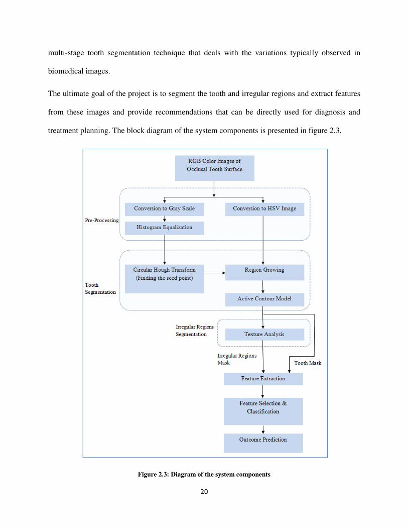
The ultimate goal of the project is to segment the tooth and irregular regions and extract features

from these images and provide recommendations that can be directly used for diagnosis and

treatment planning. The block diagram of the system components is presented in figure 2.3.

Figure 2.3: Diagram of the system components

21

Chapter 3

Tooth Surface Segmentation

3.1 Introduction

The designed computational method herein analyzes photographs captured by digital cameras

and produces predictions as to the existence and the severity of caries. The method segments the

tooth image into background, healthy enamel surface, and any irregular regions. Irregular

regions, in this study, are the regions of interest for the dentists, which show different color,

translucency and porosity. Segmentation is performed in two stages; at the first stage the tooth

surface is segmented from the background and the second step is to determine the irregular

regions within the tooth boundaries. The first step of segmentation process is described in this

chapter and the irregular region segmentation methodology is described in the next chapter.

Segmentation of tooth from the complex background is the first step in order to design a practical

dental decision support system. Given the complex backgrounds (gum, tongue, adjacent teeth,

etc.) as well as variety of tooth shapes, the tooth boundaries detection cannot be achieved by

applying either a top-down or a bottom-up approach alone. By combining a top-down and a

bottom-up approach, this method is capable of accurate detection of the tooth boundary. The

22

methodology is a novel multi-stage technique that applies a single seeded color image region

growing method and an active contour model to find the tooth boundary.

3.2 Pre-Processing

The initial color image is in RGB format. Both grayscale and HSV information will be used in

the multi stage segmentation technique; so a color space transformation is needed. In order to

convert RGB to grayscale the standard NTSC (National Television System Committee) formula

is used. The intensity is calculated directly from gamma-compressed primary intensities as a

weighted sum as described in equation 3.1.

� = 0.2990� + 0.5870� + 0.1140� (3.1)

The Hue Saturation Value (HSV) system separates color information of an image from its

intensity information. Color information is represented by Hue and Saturation, while Value

describes the brightness of an image. Hue represents basic colors, and is determined by the

dominant wavelength in the spectral distribution of light wavelengths. It is the location of the

peak in the spectral distribution. The saturation is a measure of the purity of the color, and

signifies the amount of white light mixed with the hue. It is the height of the peak relative to the

entire spectral distribution. RGB to HSV transformation is as described in equations 3.2 to 3.4.

� = arctan� √!�"#$��%#"�&�%#$�� (3.2)

' = �%&"&$�! (3.3)

( = 1 − *+�%,",$�, (3.4)

23

Histogram equalization is applied to the gray level image to improve performance in the

subsequent image processing steps. Histogram equalization reduces the effect of under and over

exposure. Histogram equalization accomplishes this by effectively spreading out the most

frequent intensity values. The gray level transformation function, T(x) is given by equations 3.5

and 3.6.

� = -��� (3.5)

�. = -��.� = ∑ 01.234 5�26 = ∑ 7.234 (3.6)

Where, x is the input image and y is the output image and k=0,1,…,L-1; L is the total number of

gray levels in the image (in this case 256); nj is the number of occurrence of a pixel with gray

level j and n is the total number of pixels in the image, so Px(j)=nj/n is the probability of

occurrence of a pixel with gray level j [39].

3.3 Initial Single Seed Selection

Conventional image segmentation techniques using region growing require initial seed selection

and recursive partitioning/ merging which has high computational cost and execution time. Also

with the pits and fissure areas and possible existence of caries inside the tooth, the conventional

image segmentation will partition the tooth area to more than one region. The tooth background

also consists of gums, tongue and adjacent teeth with different color, intensity and texture, so

with conventional region growing methods (seed selection, partitioning and merging) the image

will be partitioned into more than two regions (one for tooth area and one for background). By

selecting a single seed inside the tooth, the desired segmentation and reduction of computational

cost is possible.

24

3.3.1 Modified Circular Hough Transform

Circular Hough Transform used to find a single seed inside the tooth boundary. Circular Hough

Transform (CHT) [40-41] detects presence of circular shapes inside an image based on gradient

field of the image. The semicircular shape of tooth occlusal surface makes it possible to use CHT

to find circles which nearly contain the tooth boundary. During the process of finding the centers

and radii some inaccuracies can happen. In this application; finding the accurate circle center is

important not the radius of the circle. With the specific use of CHT some modification has been

done to adapt the original CHT to suit this research problem.

The original CHT is used to transform a set of feature points in the image space into a set of

accumulated votes in a parameter space. Then, for each feature point, votes are accumulated into

an accumulator array for all parameter combinations; the accumulation array has the same

dimension as the input image. The local maxima of accumulation array that contain the highest

number of votes indicate the presence of the circular shape.

A circle pattern is described by equation 3.6. Where (xc, yc) are the coordinates of the center and

(xp, yp) are the coordinates of any point on the circle and r is the radius of the circle.

5�8 − �96: + ��8 − �9�: = ;: (3.6)

The CHT utilizes the drawing of perpendicular lines to the edge of a curve or circle, these lines

will cross at the center of the circle. Therefore a “hot spot” is achieved at the center of that circle;

the accumulation array is calculated to identify that hot spot. In order to get the edges the

gradient of the gray scale image as described in equation 3.7 is used.

The gradient of a two-variable function (in this case intensity function f(x,y)) at each image point

is a 2D vector, with the components given by the derivatives in the horizontal (x) and vertical (y)

25

directions. At each image point f(x,y), the gradient vector points in the direction of largest

possible intensity increase, and the length of the gradient vector corresponds to the rate of change

in that direction. These gradients are less susceptible to lighting and camera changes, so

matching errors are reduced.

Gradient = ∆A = ∆B∆1 + ∆B

∆C (3.7)

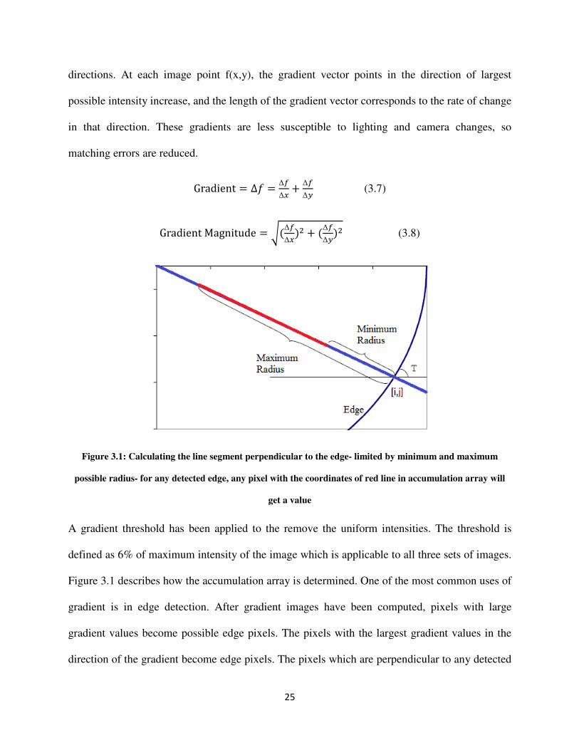
GradientMagnitude = G�∆B∆1�: + �∆B∆C�: (3.8)

Figure 3.1: Calculating the line segment perpendicular to the edge- limited by minimum and maximum

possible radius- for any detected edge, any pixel with the coordinates of red line in accumulation array will

get a value

A gradient threshold has been applied to the remove the uniform intensities. The threshold is

defined as 6% of maximum intensity of the image which is applicable to all three sets of images.

Figure 3.1 describes how the accumulation array is determined. One of the most common uses of

gradient is in edge detection. After gradient images have been computed, pixels with large

gradient values become possible edge pixels. The pixels with the largest gradient values in the

direction of the gradient become edge pixels. The pixels which are perpendicular to any detected

26

edge and are within (Minimum Radius, Maximum Radius) range will get a value in

accumulation array. Another level of thresholding applied to accumulation array value, where

any value which is less than mean of accumulation array values is removed. With the application

of this threshold local minima with small weights which cause false hot spots and thus false

detected circles are avoided. The output of CHT will be a set of circle centers and circle radii.

Basically the detected circle’s radius can be anything, even larger than the image size. A smaller

range of radii would save computational time and memory. In this application the minimum and

maximum radii of circles are defined as follows:

MinimumRadius = 1 10K LMNOOPLQRSMPTLSUTUAQℎPSMNWP (3.9)

MaximumRadius = ON;WPLQRSMPTLSUTUAQℎPSMNWP (3.10)

The definition of minimum radius is heuristic and based on this idea that the tooth of interest

should be “conceptually obvious” in the image. The output of CHT is a set of N different

parameter triplets (xc, yc, r), where N is the number of detected circles and (xc, yc, r) are circle

center dimensions and radius.

To set the seed point, first any circle center which is outside the borders of the image has been

removed; the rationale behind this is that the tooth of interest with semi-circular shape should be

inside the tooth and any circular shape with a center outside the borders of the image is either a

part of an adjacent tooth which should not be used. Then the vector sum of all remained circle

centers fall inside the tooth and will be used as the initial seed for region growing step. The CHT

applied to the grayscale conversion of the tooth image.

27

Modification to original CHT for the application:

1- Minimum and maximum radius definition with regards to the application to reduce the

computational cost.

2- The method of selection and calculation of final seed point with regards to the definition

of tooth of interest.

3- Apply two levels of thresholding; first to the gradient values and second to the

accumulation array values to reduce the false hot spots with regards to the application.

3.4 Color Image Seeded Region Growing

Seeded region growing (SRG) is a hybrid method. It starts with an assigned seed, and the region

is grown by merging a pixel into its nearest neighboring seeded region. Considering local

information such as regions similarity, boundaries and smoothness makes SRG robust to a large

variety of images. Each ROI requires its own seed initialization; in this application there is one

ROI, the whole tooth surface. Thus, one initial seed is requires, which is the output of CHT.

Once the seed is determined, then the region is grown in the neighborhood of the pixels from the

seed. HSV color model which is corresponding to human color perception has been used for

region growing. For any pixel at (x,y) a 4- pixel neighbourhood N(x, y)={(x−1,y), (x, y+1),

(x+1, y), (x, y−1)} is defined and used for region growing.

Figure 3.2: 4-Neighbourhood

28

The region is iteratively grown by comparing all unallocated neighboring pixels to the region. A

measure of similarity explained later for HSV space. The pixel with the smallest difference

measured is allocated to the respective region. This process stops when the difference measure

between region mean and new pixel become larger than a certain threshold (MaxDistance). The

obtained image is the initial segmented tooth image [31].

YN��SLQNTZP = MPNT�ℎL[SMNWP� + LQNTRN;RRP[SNQSUT�ℎL[SMNWP� (3.12)

3.4.1 Measure of Similarity for HSV Space

For a pixel at (x,y) the color information is �ℎ��, ��, L��, ��, [��, ���. The average value of

color over the neighborhood N(x,y) is �ℎ��, ��, L��, ��, [��, ���. Equation 3.12 computes the distance between �ℎ��, ��, L��, ��, [��, ��� and�ℎ��, ��, L��, ��, [��, ���.

R��, �� = \�[ − [�: + �L cos�ℎ� − Lcos�ℎ_��: + �L sin�ℎ� − Lsin�ℎ_��: (3.12)

The value of d(x,y) over N(x,y) defined as a measure of smoothness. The output of region

growing is almost near the tooth boundary but it needs another refinement to exactly locate the

true boundary of the tooth.

3.5 Active Contour Model

For almost all the in-vitro images, the two last steps of segmentation were able to segment the

tooth but for in-vivo images, yet another step is needed to segment the tooth. The output of

region growing has been used as the initial active contour and the gray level image has been used

as the input image. An active contour model is a parametric contour that deforms over a series of

iterations. A parameter x(s,t) along with the contour therefore depends on two parameters s

(contour space parameter) and t (time parameter). The contour is influenced by internal and

external constraints, and by image forces. Internal forces constraints give the model tension and

29

stiffness. External constraints come from high-level sources such as human (in this case region

growing algorithm). Image energy is used to drive the model towards salient features such as

light and dark regions, edges, and terminations.

Figure 3.3: An Active Contour Model, over a series of iterations, the active contour moves into alignment

with the nearest salient feature, in this case an edge

A final solution is given by the minimum total energy of the snake, which is the result of

equation 3.13. Where Eint and Eext are the internal and external energy of ACM, respectively. The

internal energy is given by the membrane energy sum. u(s) is the curve of ACM which has been

created by sampling 50 points over the edge of region growing algorithm output.

abc = d e +f5g�L�6 + `h1f5g�L�6iRL�4 (3.13)

g�L� = ���L�, ��L�� (3.14)

30

Chapter 4

Irregular Region Identification

4.1 Introduction

The irregular regions are defined by spatial statistics as well as texture analysis, adding texture

information empowers the system to not only focus on visible changes in the enamel, which is

the region of interest for the dentists but also focus on the textural changes which are not visible

and usually are only detectable with tactile examination. These image processing features are

designed to best represent visual irregularities examined by the dentists during visual/visuo-

tactile examination. These features are then used to detect the existence and severity of caries in

the identified irregular regions.

4.2 Texture Analysis

The irregular regions within the tooth boundaries were segmented by the application of texture

assessment through the use of morphology operators. After finding the tooth boundaries, the

irregular regions are identified. Haar Discrete Wavelet Transform (DWT) is used to do the

texture analysis [42]. The Haar wavelet’s mother wavelet function ψ (t) described in equation 4.1

and its scaling function Φ(t) described in equation 4.2.

Ψ�Q� = j 10 ≤ Q ≤ �:−1 �: ≤ Q ≤ 10UQℎP;lSLP m (4.1)

31

n,.(t)=2op n�2Q − q�, Q ∊ s (4.2)

To start irregular region detection, a background mask applied to the color image, meaning all

the operations just applied to the tooth boundary. The mean value of the first component of color

space (Mean of Hue) is calculated then a black and white mask generated by applying the Mean

of RED threshold value. This black and white mask is convolved by a low pass filter of size 9×9

to smooth it and reduce the number of connected components. Morphological operations are

applied to remove the spurious edges and objects with area smaller than 3×3 squares. The

resulted black and white mask then applied to the gray scale image. Morphological operations

are a collection of non-linear operations related to the shape or morphology of features in an

image. Morphological operations rely only on the relative ordering of pixel values, not on their

numerical values, and therefore are especially suited to the processing of binary images.

Morphological operations probe an image with a small shape or template called a structuring

element. The structuring element is positioned at all possible locations in the image and it is

compared with the corresponding neighborhood of pixels then test whether the element fits

within the neighborhood or not. In this application the structuring element is a 3×3 square. The

3×3 square probes the whole binary image; each of its pixels is associated with the

corresponding pixel of the neighborhood under the structuring element. The structuring elements

will set to ones if the majority of corresponding pixel of the neighborhood are ones (5 or more

ones) otherwise they will set to zeros.

Wavelet transform applied to the output of the previous step in order to reconstruct the image

using only the approximation matrix. Haar wavelet is selected as the mother wavelet because of

its discontinuity and intrinsic ability to accentuate transitions between gray levels. Then the mean

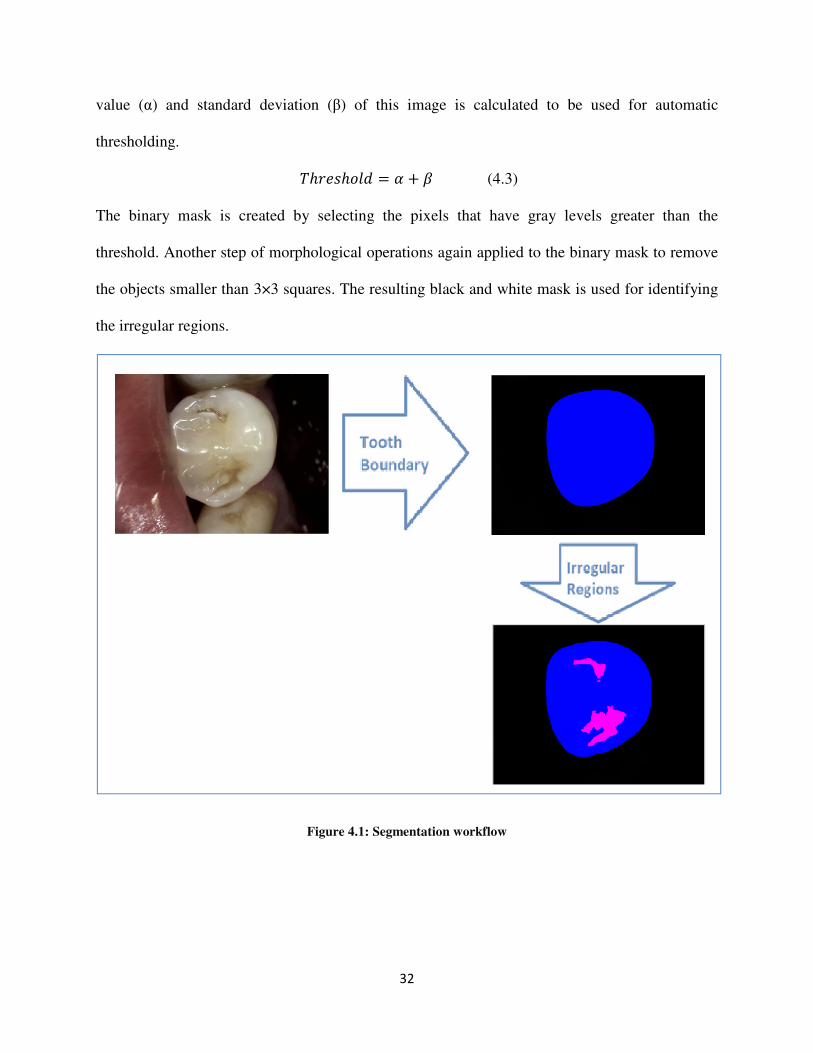
32

value (α) and standard deviation (β) of this image is calculated to be used for automatic

thresholding.

-ℎ;PLℎUOR = t + u (4.3)

The binary mask is created by selecting the pixels that have gray levels greater than the

threshold. Another step of morphological operations again applied to the binary mask to remove

the objects smaller than 3×3 squares. The resulting black and white mask is used for identifying

the irregular regions.

Figure 4.1: Segmentation workflow

33

Chapter 5

Feature Selection and Classification

5.1Feature Extraction

The features are measures calculated from 10×10 windows scrolled over the entire enamel

surface and the detected irregular region, separately. Feature extraction over windows presents

local information in feature space. Experimental testing revealed that 10×10 window size

performed best for this application. Window sizes ranging from 7×7 to 12×12 were tested and

10×10 had the best performance by visual evaluation and also final accuracy. The designed

system extracted 87 region-based and pixel-based features from both enamel (as control) and the

irregular regions separately based on color space and Fourier transforms. Each feature is

described below.

Mean of matrix elements in a 10×10 window calculated as described in equation 5.1.

Meanofmatrixelements = ��44∑ �4+3� ∑ A�S, x��423� (5.1)

An image gradient, which described in equation 5.2 is a directional change in the intensity or

color in the image.

Gradient = ∆A = ∆B∆1 + ∆B

∆C (5.2)

34

Table 5.1 describes how the features created in 10 by 10 windows level and how their statistical

measures create the final feature pool for each image. Subscript 2 means the operation has been

done in 10 by 10 windows level and subscript 1 means has been done in global level. The table

shows 43 possible features for an image. These 43 features were calculated for the tooth surface

except irregular regions mask; an example of such a mask is the blue regions in figure 7.15. The

other 43 features were calculated for the irregular regions mask; an example of such a mask is

the red regions in figure 7.15. The ratio of the total area of irregular regions to the total tooth area

is the last feature .Finally 87 features have been calculated for each image.

First

Component

of RGB

Color Space

(RED)

Second

Component

of RGB

Color Space

(GREEN)

First

Component

of RGB

Color Space

(BLUE)

First

Component

of HSV

Color Space

(Hue)

Second

Component

of HSV

Color Space

(Saturation)

First

Component

of HSV

Color Space

(Value)

Fourier

Transform

Mean1(Mean2) X X X X X X X

Std1(Mean2) X X X X X X

Median1(Mean2) X X X X X X

Maximum1(Mean2) X X X X X X

Maximum1(Gradient2) X X X X X X

Mean1(Maximum2) X X X X X X

Mean1(Minimum2) X X X X X X

Table 5.1: Feature Extraction

5.2 Feature Selection and Classification

While the dataset for this research has representation in each of the ICDAS categories, it does

not have sufficient examples of some of ICDAS scores to warrant individual score classification.

ICDAS Scoring System has seven scores, defining a state of caries development. 0: Sound Tooth

– 1: First visual Change in Enamel – 2: Distinct Visual Change in Enamel- 3: Localized Enamel

Breakdown- 4: Underlying Dentin Shadow- 5: Distinct Cavity with Visible Dentin- 6: Extensive

Cavity with Visible Dentin. Thus the traditional ICDAS classification has been modified for this

35

research to specify: Sound occlusal (ICDAS Score 0), Initial caries (ICDAS Score 1 or 2),

Moderate caries (ICDAS Score 3-5), severe caries (ICDAS Score 6) [43].

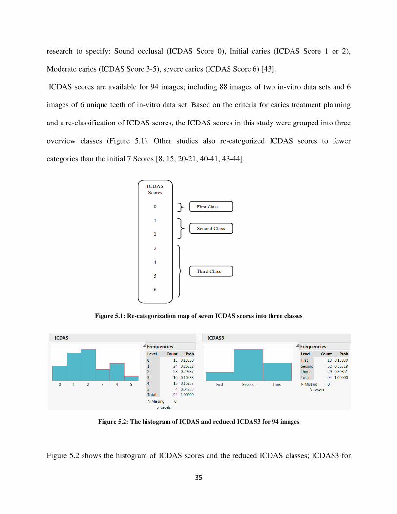
ICDAS scores are available for 94 images; including 88 images of two in-vitro data sets and 6

images of 6 unique teeth of in-vitro data set. Based on the criteria for caries treatment planning

and a re-classification of ICDAS scores, the ICDAS scores in this study were grouped into three

overview classes (Figure 5.1). Other studies also re-categorized ICDAS scores to fewer

categories than the initial 7 Scores [8, 15, 20-21, 40-41, 43-44].

Figure 5.1: Re-categorization map of seven ICDAS scores into three classes

Figure 5.2: The histogram of ICDAS and reduced ICDAS3 for 94 images

Figure 5.2 shows the histogram of ICDAS scores and the reduced ICDAS classes; ICDAS3 for

36

the classification data set (94 images). It is clear that ICDAS3 is an imbalance data set. The

classifier constructed to minimize the overall error rate; it will tend to focus more on the

prediction accuracy of the majority class, which often results in poor accuracy for the minority

classes. There are multiple approaches to cope with imbalance data sets, such as under sampling,

over sampling and cost sensitive learning. For our size of data set, cost sensitive learning is the

best approach. Since the classifier tends to be biased towards the majority class, a heavier penalty

on misclassifying the minority class should be defined. A weight has been assigned to each class,

with the minority class given larger weight (i.e., higher mis- classification cost). A weighted

random forest classifier used to train the final classification model.

In order to compare performance of the ICDAS based caries detection system, another system

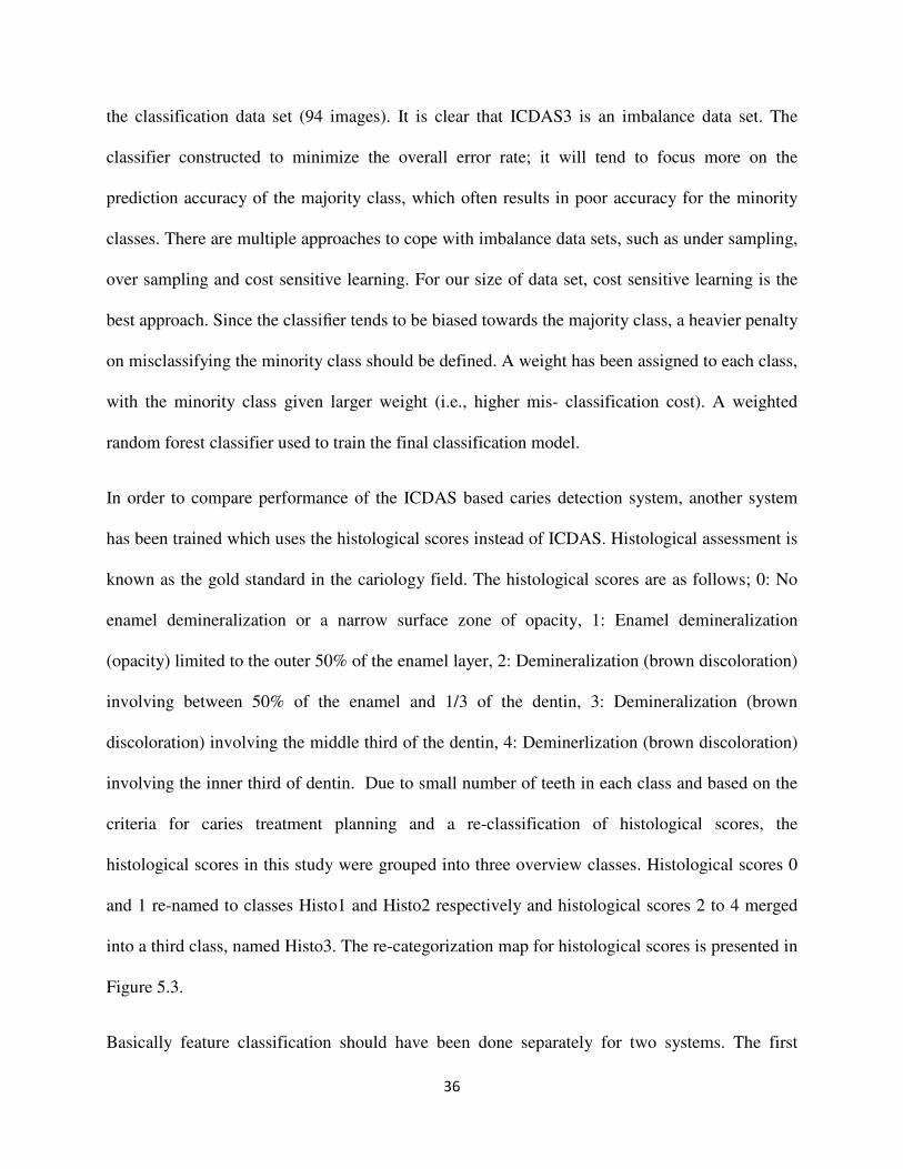
has been trained which uses the histological scores instead of ICDAS. Histological assessment is

known as the gold standard in the cariology field. The histological scores are as follows; 0: No

enamel demineralization or a narrow surface zone of opacity, 1: Enamel demineralization

(opacity) limited to the outer 50% of the enamel layer, 2: Demineralization (brown discoloration)

involving between 50% of the enamel and 1/3 of the dentin, 3: Demineralization (brown

discoloration) involving the middle third of the dentin, 4: Deminerlization (brown discoloration)

involving the inner third of dentin. Due to small number of teeth in each class and based on the

criteria for caries treatment planning and a re-classification of histological scores, the

histological scores in this study were grouped into three overview classes. Histological scores 0

and 1 re-named to classes Histo1 and Histo2 respectively and histological scores 2 to 4 merged

into a third class, named Histo3. The re-categorization map for histological scores is presented in

Figure 5.3.

Basically feature classification should have been done separately for two systems. The first

37

system uses ICDAS scores and the second system uses histological scores.

Figure 5.3: Re-categorization map for Ekstrand histological scores: five histological scores mapping into

three classes

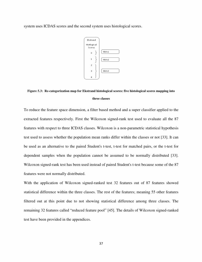
To reduce the feature space dimension, a filter based method and a super classifier applied to the

extracted features respectively. First the Wilcoxon signed-rank test used to evaluate all the 87

features with respect to three ICDAS classes. Wilcoxon is a non-parametric statistical hypothesis

test used to assess whether the population mean ranks differ within the classes or not [33]. It can

be used as an alternative to the paired Student's t-test, t-test for matched pairs, or the t-test for

dependent samples when the population cannot be assumed to be normally distributed [33].

Wilcoxon signed-rank test has been used instead of paired Student's t-test because some of the 87

features were not normally distributed.

With the application of Wilcoxon signed-ranked test 32 features out of 87 features showed

statistical difference within the three classes. The rest of the features; meaning 55 other features

filtered out at this point due to not showing statistical difference among three classes. The

remaining 32 features called “reduced feature pool” [45]. The details of Wilcoxon signed-ranked

test have been provided in the appendices.

38

A heuristic super classifier method used to select the high ranked features as well as a

classification model [45]. Super Classifier encompasses four classification methods to perform

the classification task including C4.5 decision tree [46], Support Vector Machine (SVM) [47],

Random Forest classifier [48] and Artificial Neural Network classifier [30]. These four

classification methods showed successful performance in medical decision support systems. The

super classifier uses the ten-fold cross validation to avoid over-fitting. For each image a reduced

feature pool of 32 are available. Feature ranking was done by using information gain ratio

method; ranking has been assigned to the features according to relevance to the categories. An

extensive search has been performed to find the best features and the best classifier. Through the

extensive search the number of high ranked features varied from 5 to 32 for each as well as the

classification methods and classification parameters. Five was chosen as the minimum number of

selected features because any less than that would not provide sufficient information to classify

items into three classes. Figure 5.4 describes the multi stage feature selection and classification

algorithm. Ten-Fold cross validation was used to validate the results in all cases. Based on the

best performance, Random Forest Classifier with the reported setting was selected for both

systems.

Ten-fold cross validation, which is a standard process to assess the accuracy and reliability of the

models developed from data, was used to validate the resulting computational model. In ten-fold

cross-validation, the combined dataset was randomly partitioned into 10 subsets. Of the 10

subsets, a single subset was kept as the validation set for testing the model, and the remaining 9

subsets were used for training of the model. Cross-validation was then repeated 10 times (the

folds) in a “round-robin” process, with each of the 10 subsets used exactly once as the validation

sets.

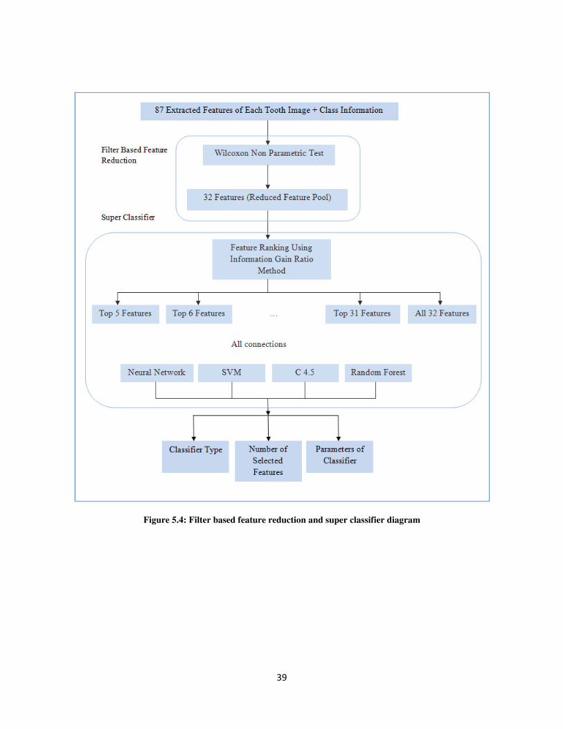
39

Figure 5.4: Filter based feature reduction and super classifier diagram

40

Chapter 6

Description of Data Set

6.1 Introduction

The data used in this study consist of three sets of color images; while all sets of images contain

occlusal surface of a molar or pre-molar teeth. All the teeth are free from restoration on occlusal

surface. The first two data sets are in-vitro images taken from extracted teeth in different

experiments. The third data set consists of in-vivo images of a molar or pre-molar tooth of

interest and the adjacent teeth.

6.2 In-Vitro Data Sets

The in-vitro data set consists of 88 images of the occlusal surface of an extracted tooth, one

image per tooth surface. The data set consists of images of teeth with different stages of caries.

In-vitro data set consists of 72 and 16 images taken in two different experiments.

6.2.1 First In-Vitro Data Set

The first in-vitro data set includes 72 images of size 1440×2160×3 with a light blue background.

Where the first two image size dimensions represent pixel size and the third dimension

represents RGB (Red, Green, Blue). The images were taken with digital camera with 1440×2160

resolution. Each extracted tooth was examined and scored by ICDAS experts in a previous

cariology study conducted in 2001 [19]. Each image was scored based on ICDAS [19] by

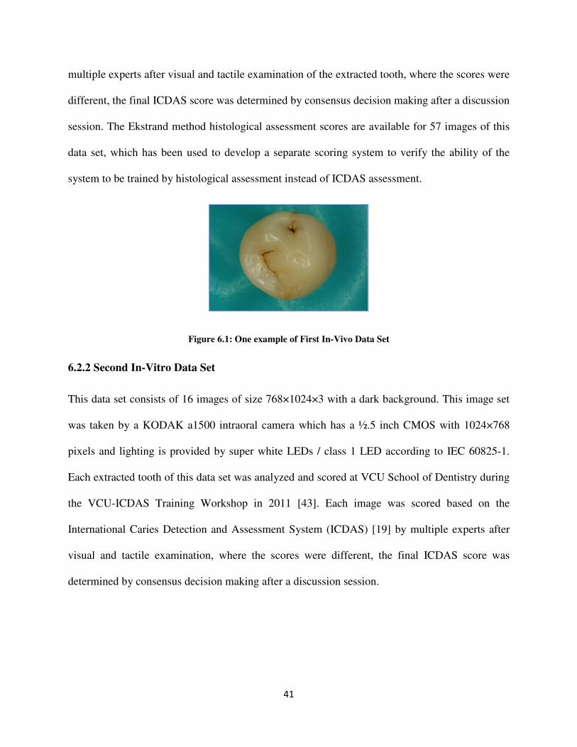
41

multiple experts after visual and tactile examination of the extracted tooth, where the scores were

different, the final ICDAS score was determined by consensus decision making after a discussion

session. The Ekstrand method histological assessment scores are available for 57 images of this

data set, which has been used to develop a separate scoring system to verify the ability of the

system to be trained by histological assessment instead of ICDAS assessment.

Figure 6.1: One example of First In-Vivo Data Set

6.2.2 Second In-Vitro Data Set

This data set consists of 16 images of size 768×1024×3 with a dark background. This image set

was taken by a KODAK a1500 intraoral camera which has a ½.5 inch CMOS with 1024×768

pixels and lighting is provided by super white LEDs / class 1 LED according to IEC 60825-1.

Each extracted tooth of this data set was analyzed and scored at VCU School of Dentistry during

the VCU-ICDAS Training Workshop in 2011 [43]. Each image was scored based on the

International Caries Detection and Assessment System (ICDAS) [19] by multiple experts after

visual and tactile examination, where the scores were different, the final ICDAS score was

determined by consensus decision making after a discussion session.

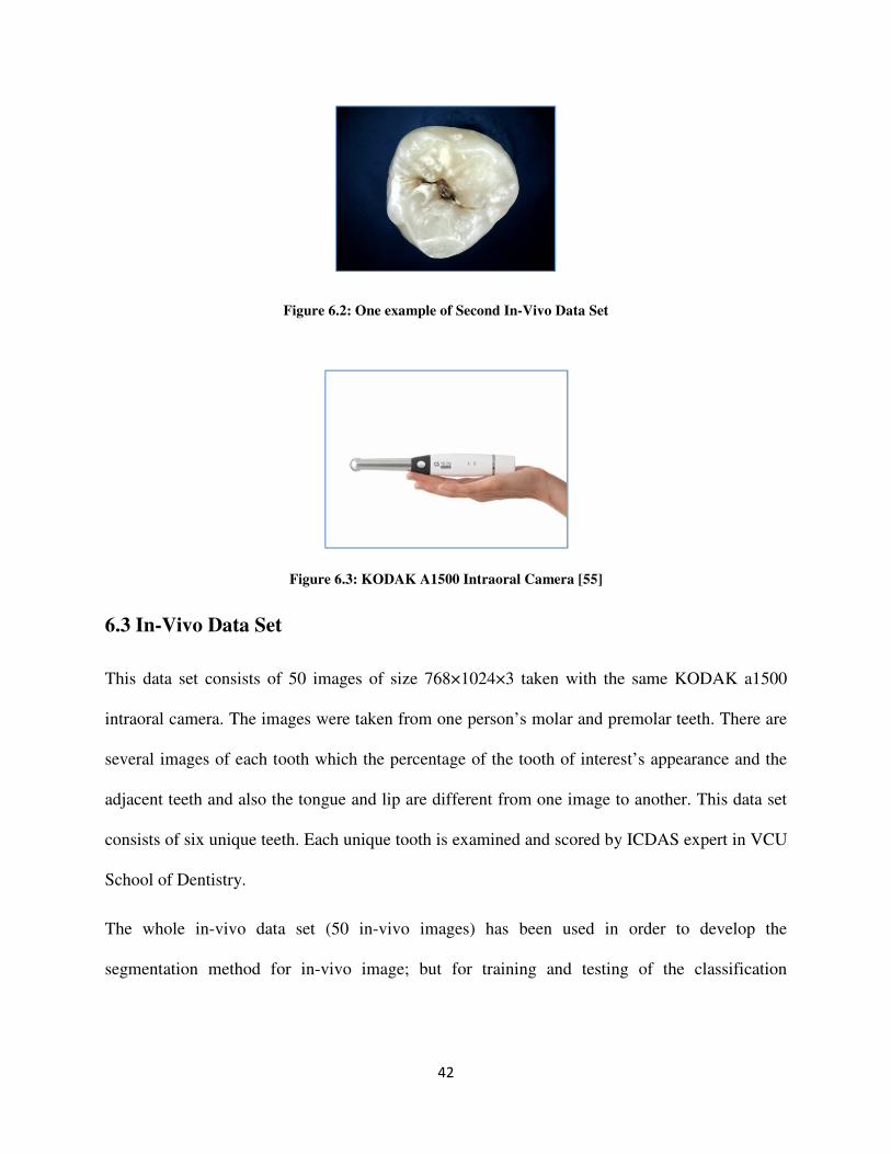
42

Figure 6.2: One example of Second In-Vivo Data Set

Figure 6.3: KODAK A1500 Intraoral Camera [55]

6.3 In-Vivo Data Set

This data set consists of 50 images of size 768×1024×3 taken with the same KODAK a1500

intraoral camera. The images were taken from one person’s molar and premolar teeth. There are

several images of each tooth which the percentage of the tooth of interest’s appearance and the

adjacent teeth and also the tongue and lip are different from one image to another. This data set

consists of six unique teeth. Each unique tooth is examined and scored by ICDAS expert in VCU

School of Dentistry.

The whole in-vivo data set (50 in-vivo images) has been used in order to develop the

segmentation method for in-vivo image; but for training and testing of the classification

43

algorithm only one image per tooth (6 images) was used to keep the consistency with in-vitro

images. As it was discussed earlier in-vivo data set consists of 50 images of 6 unique teeth.

The tooth of interest should be “conceptually obvious” in the image, which means an image can

include the tooth of interest’s occlusal surface and adjacent teeth and tissues but the image

should not include two whole occlusal surfaces of two teeth in a way that it’s hard to tell which

tooth is the subject of evaluation.

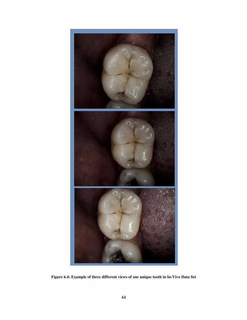
44

Figure 6.4: Example of three different views of one unique tooth in In-Vivo Data Set

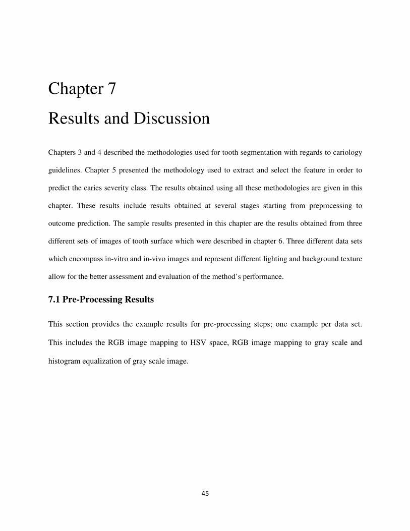
45

Chapter 7

Results and Discussion

Chapters 3 and 4 described the methodologies used for tooth segmentation with regards to cariology

guidelines. Chapter 5 presented the methodology used to extract and select the feature in order to

predict the caries severity class. The results obtained using all these methodologies are given in this

chapter. These results include results obtained at several stages starting from preprocessing to

outcome prediction. The sample results presented in this chapter are the results obtained from three

different sets of images of tooth surface which were described in chapter 6. Three different data sets

which encompass in-vitro and in-vivo images and represent different lighting and background texture

allow for the better assessment and evaluation of the method’s performance.

7.1 Pre-Processing Results

This section provides the example results for pre-processing steps; one example per data set.

This includes the RGB image mapping to HSV space, RGB image mapping to gray scale and

histogram equalization of gray scale image.

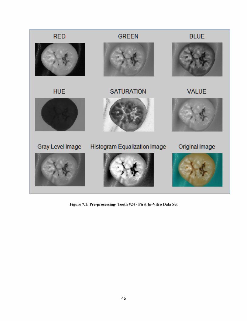
46

Figure 7.1: Pre-processing- Tooth #24 - First In-Vitro Data Set

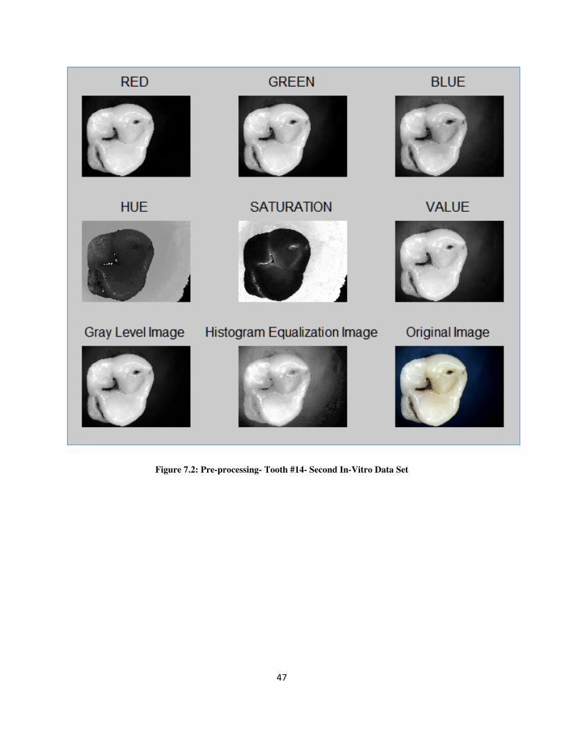
47

Figure 7.2: Pre-processing- Tooth #14- Second In-Vitro Data Set

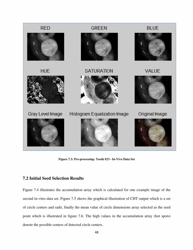
48

Figure 7.3: Pre-processing- Tooth #23 - In-Vivo Data Set

7.2 Initial Seed Selection Results

Figure 7.4 illustrates the accumulation array which is calculated for one example image of the

second in-vitro data set. Figure 7.5 shows the graphical illustration of CHT output which is a set

of circle centers and radii, finally the mean value of circle dimensions array selected as the seed

point which is illustrated in figure 7.6. The high values in the accumulation array (hot spots)

denote the possible centers of detected circle centers.

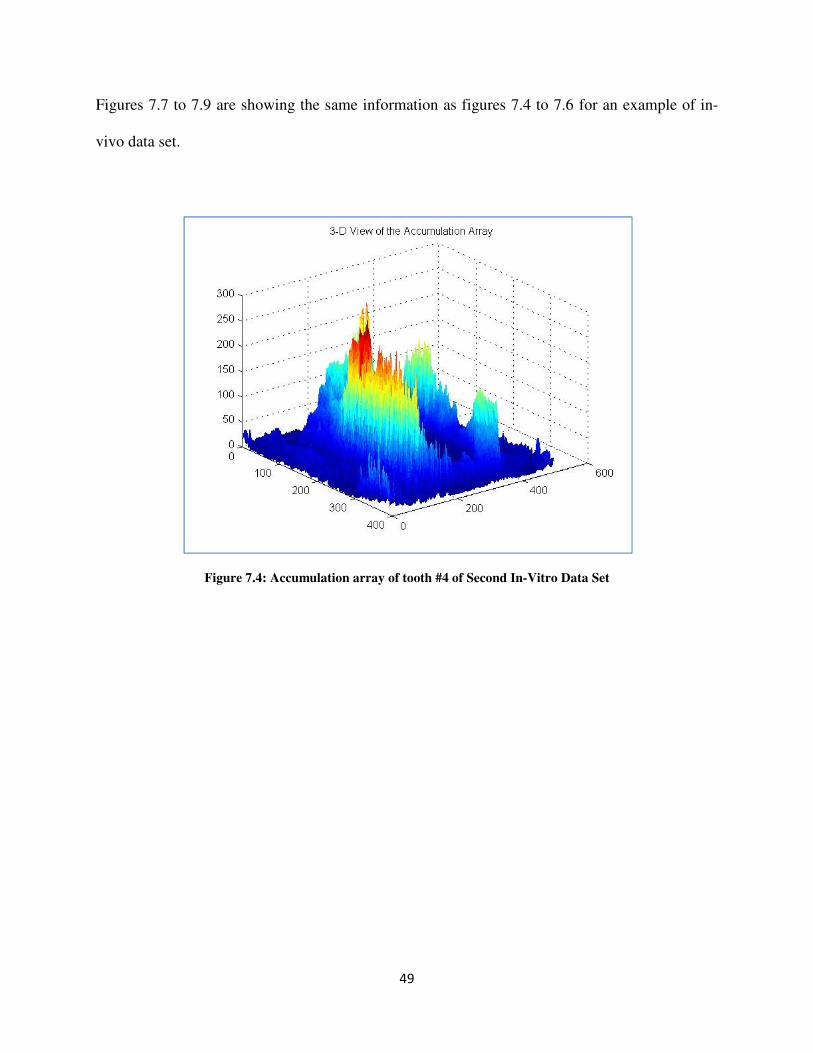
49

Figures 7.7 to 7.9 are showing the same information as figures 7.4 to 7.6 for an example of in-

vivo data set.

Figure 7.4: Accumulation array of tooth #4 of Second In-Vitro Data Set

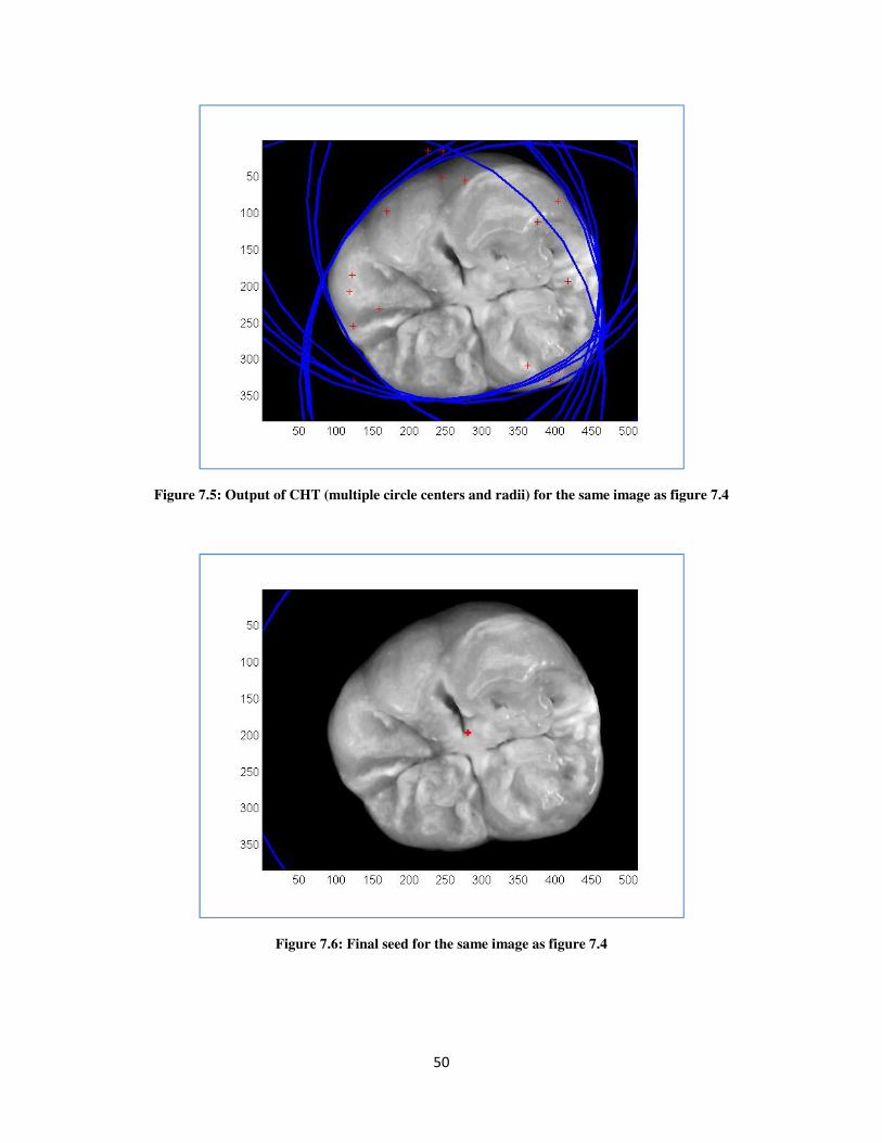
50

Figure 7.5: Output of CHT (multiple circle centers and radii) for the same image as figure 7.4

Figure 7.6: Final seed for the same image as figure 7.4

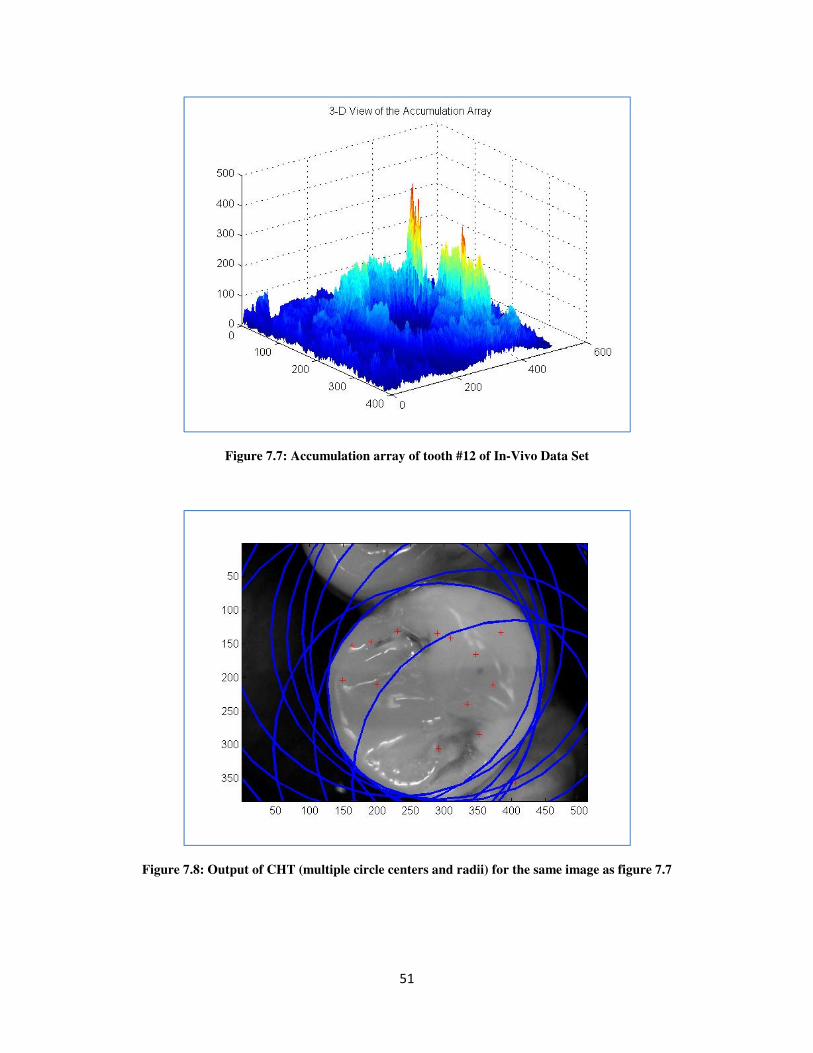
51

Figure 7.7: Accumulation array of tooth #12 of In-Vivo Data Set

Figure 7.8: Output of CHT (multiple circle centers and radii) for the same image as figure 7.7

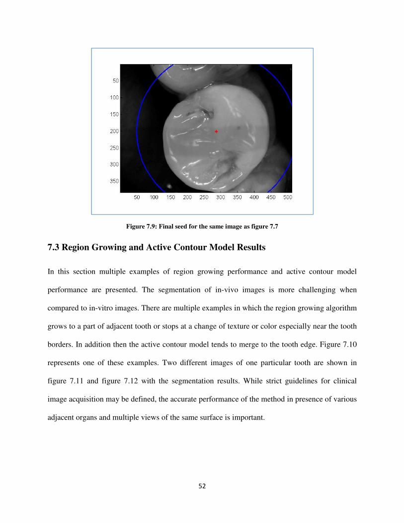
52

Figure 7.9: Final seed for the same image as figure 7.7

7.3 Region Growing and Active Contour Model Results

In this section multiple examples of region growing performance and active contour model

performance are presented. The segmentation of in-vivo images is more challenging when

compared to in-vitro images. There are multiple examples in which the region growing algorithm

grows to a part of adjacent tooth or stops at a change of texture or color especially near the tooth

borders. In addition then the active contour model tends to merge to the tooth edge. Figure 7.10

represents one of these examples. Two different images of one particular tooth are shown in

figure 7.11 and figure 7.12 with the segmentation results. While strict guidelines for clinical

image acquisition may be defined, the accurate performance of the method in presence of various

adjacent organs and multiple views of the same surface is important.

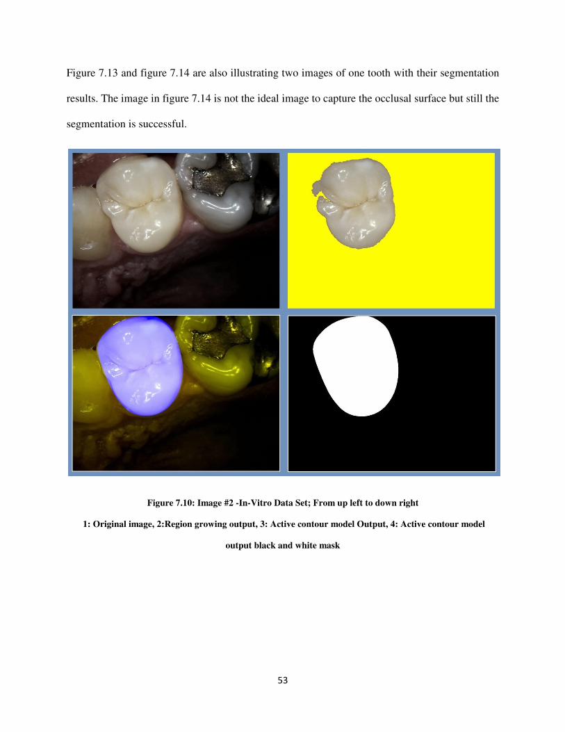
53

Figure 7.13 and figure 7.14 are also illustrating two images of one tooth with their segmentation

results. The image in figure 7.14 is not the ideal image to capture the occlusal surface but still the

segmentation is successful.

Figure 7.10: Image #2 -In-Vitro Data Set; From up left to down right

1: Original image, 2:Region growing output, 3: Active contour model Output, 4: Active contour model

output black and white mask

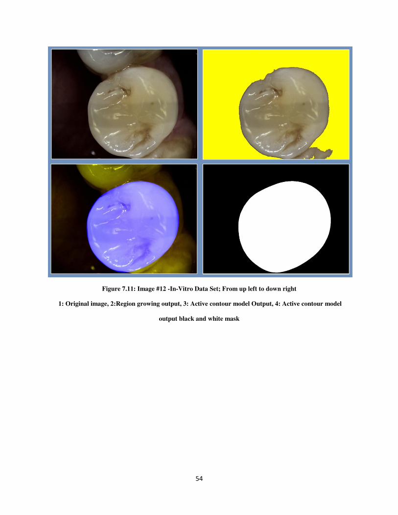
54

Figure 7.11: Image #12 -In-Vitro Data Set; From up left to down right

1: Original image, 2:Region growing output, 3: Active contour model Output, 4: Active contour model

output black and white mask

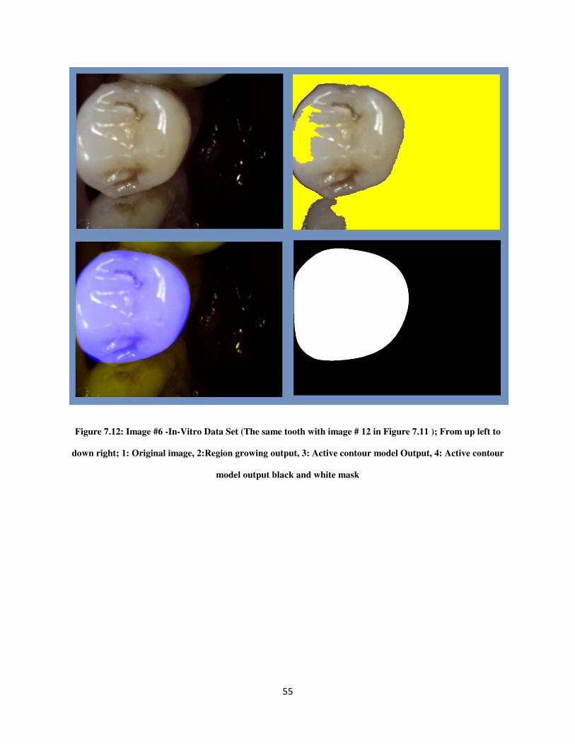
55

Figure 7.12: Image #6 -In-Vitro Data Set (The same tooth with image # 12 in Figure 7.11 ); From up left to

down right; 1: Original image, 2:Region growing output, 3: Active contour model Output, 4: Active contour

model output black and white mask

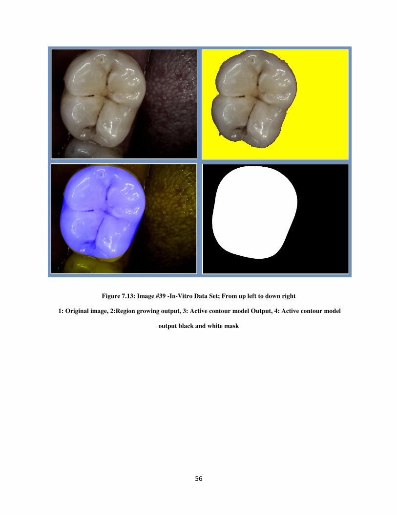
56

Figure 7.13: Image #39 -In-Vitro Data Set; From up left to down right

1: Original image, 2:Region growing output, 3: Active contour model Output, 4: Active contour model

output black and white mask

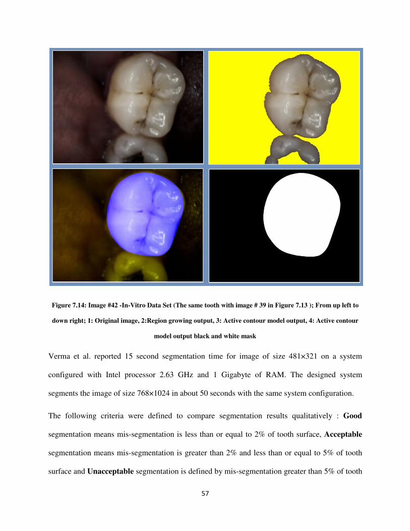
57

Figure 7.14: Image #42 -In-Vitro Data Set (The same tooth with image # 39 in Figure 7.13 ); From up left to

down right; 1: Original image, 2:Region growing output, 3: Active contour model output, 4: Active contour

model output black and white mask

Verma et al. reported 15 second segmentation time for image of size 481×321 on a system

configured with Intel processor 2.63 GHz and 1 Gigabyte of RAM. The designed system

segments the image of size 768×1024 in about 50 seconds with the same system configuration.

The following criteria were defined to compare segmentation results qualitatively : Good

segmentation means mis-segmentation is less than or equal to 2% of tooth surface, Acceptable

segmentation means mis-segmentation is greater than 2% and less than or equal to 5% of tooth

surface and Unacceptable segmentation is defined by mis-segmentation greater than 5% of tooth

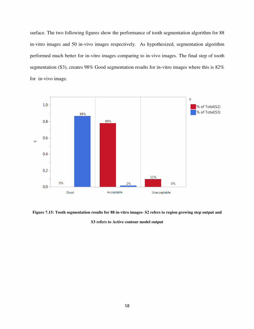
58

surface. The two following figures show the performance of tooth segmentation algorithm for 88

in-vitro images and 50 in-vivo images respectively. As hypothesized, segmentation algorithm

performed much better for in-vitro images comparing to in-vivo images. The final step of tooth

segmentation (S3), creates 98% Good segmentation results for in-vitro images where this is 82%

for in-vivo image.

Figure 7.15: Tooth segmentation results for 88 in-vitro images- S2 refers to region growing step output and

S3 refers to Active contour model output

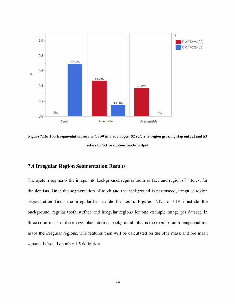
59

Figure 7.16: Tooth segmentation results for 50 in-vivo images- S2 refers to region growing step output and S3

refers to Active contour model output

7.4 Irregular Region Segmentation Results

The system segments the image into background, regular tooth surface and region of interest for

the dentists. Once the segmentation of tooth and the background is performed, irregular region

segmentation finds the irregularities inside the tooth. Figures 7.17 to 7.19 illustrate the

background, regular tooth surface and irregular regions for one example image per dataset. In

three color mask of the image, black defines background, blue is the regular tooth image and red

maps the irregular regions. The features then will be calculated on the blue mask and red mask

separately based on table 1.5 definition.

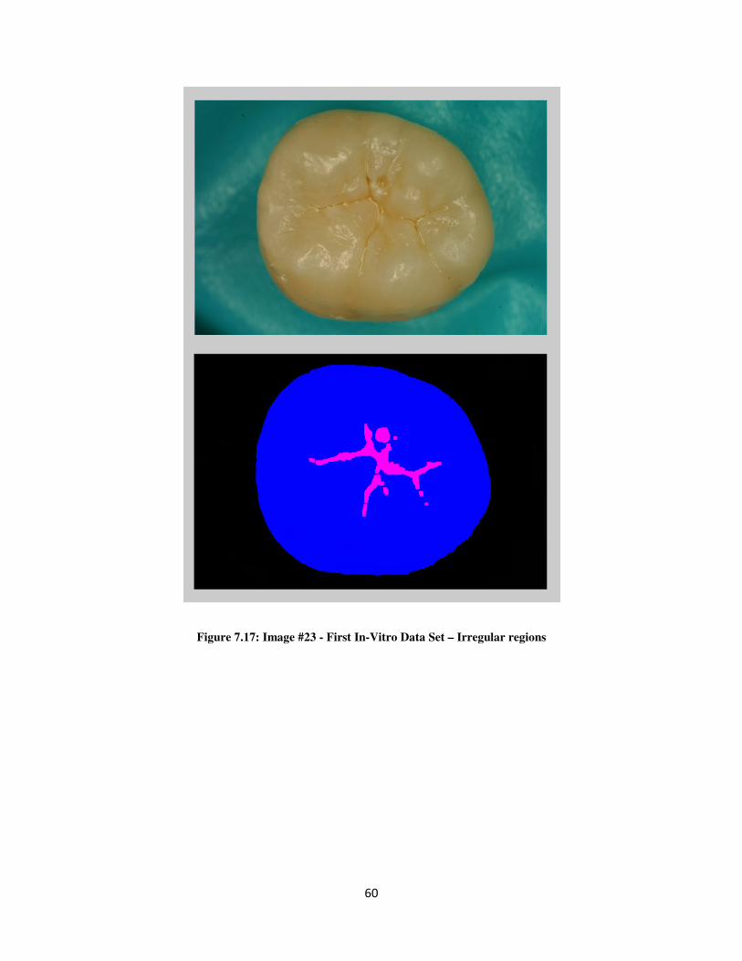
60

Figure 7.17: Image #23 - First In-Vitro Data Set – Irregular regions

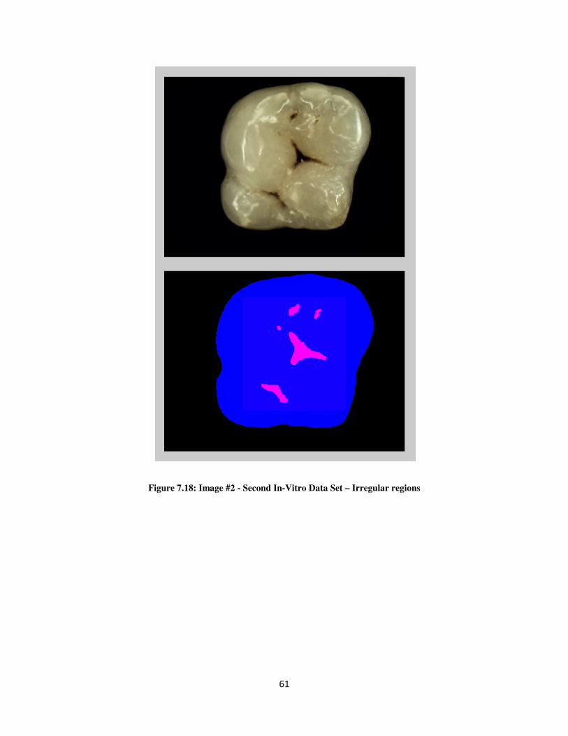
61

Figure 7.18: Image #2 - Second In-Vitro Data Set – Irregular regions

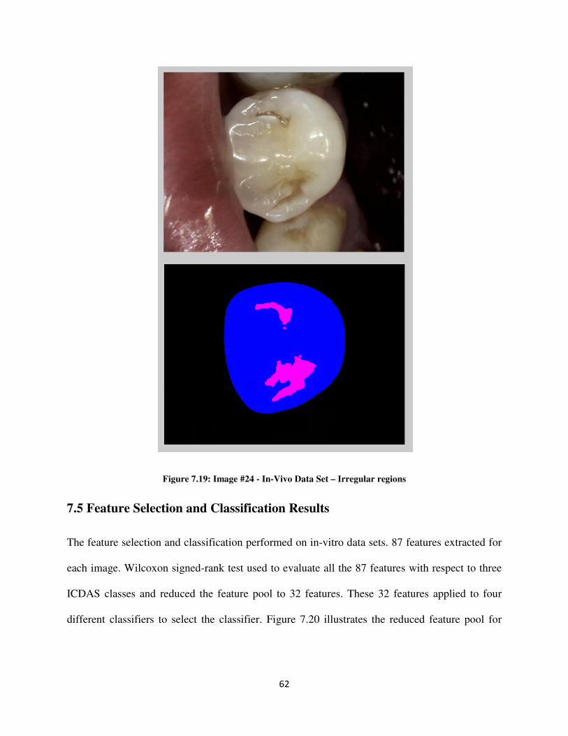
62

Figure 7.19: Image #24 - In-Vivo Data Set – Irregular regions

7.5 Feature Selection and Classification Results

The feature selection and classification performed on in-vitro data sets. 87 features extracted for

each image. Wilcoxon signed-rank test used to evaluate all the 87 features with respect to three

ICDAS classes and reduced the feature pool to 32 features. These 32 features applied to four

different classifiers to select the classifier. Figure 7.20 illustrates the reduced feature pool for

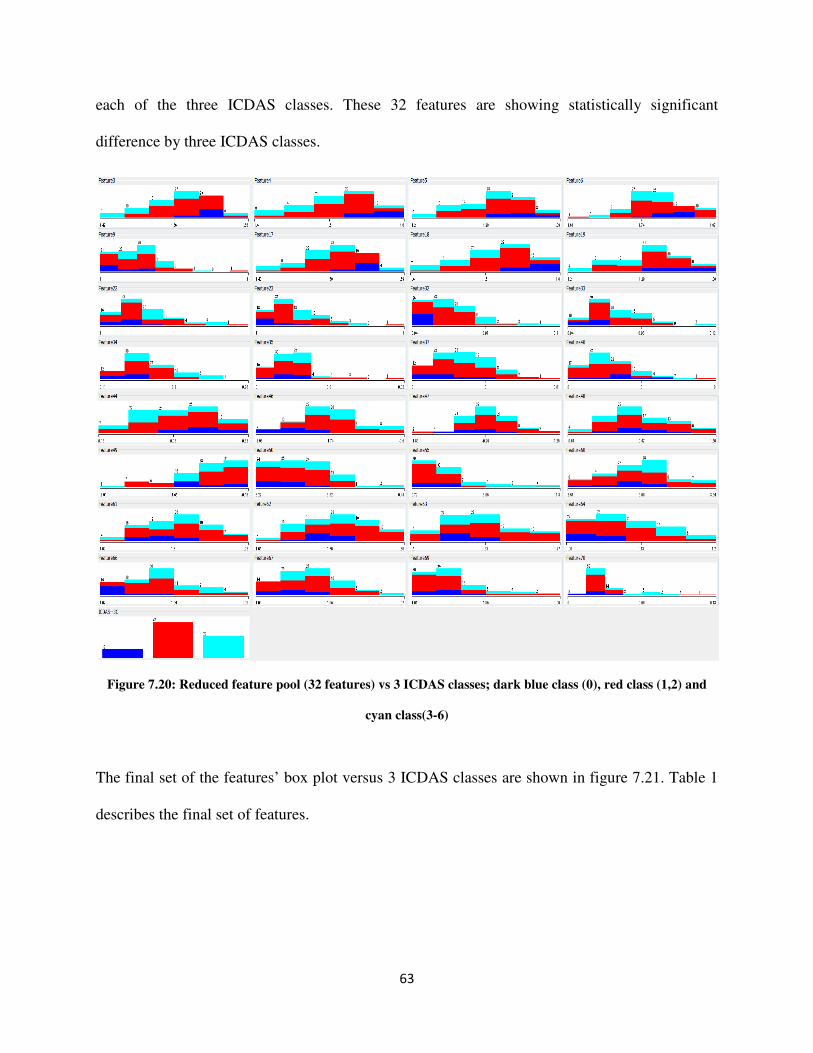
63

each of the three ICDAS classes. These 32 features are showing statistically significant

difference by three ICDAS classes.

Figure 7.20: Reduced feature pool (32 features) vs 3 ICDAS classes; dark blue class (0), red class (1,2) and

cyan class(3-6)

The final set of the features’ box plot versus 3 ICDAS classes are shown in figure 7.21. Table 1

describes the final set of features.

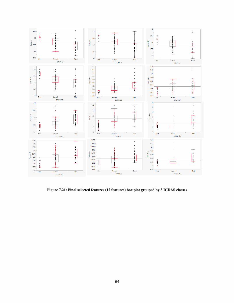
64

Figure 7.21: Final selected features (12 features) box plot grouped by 3 ICDAS classes

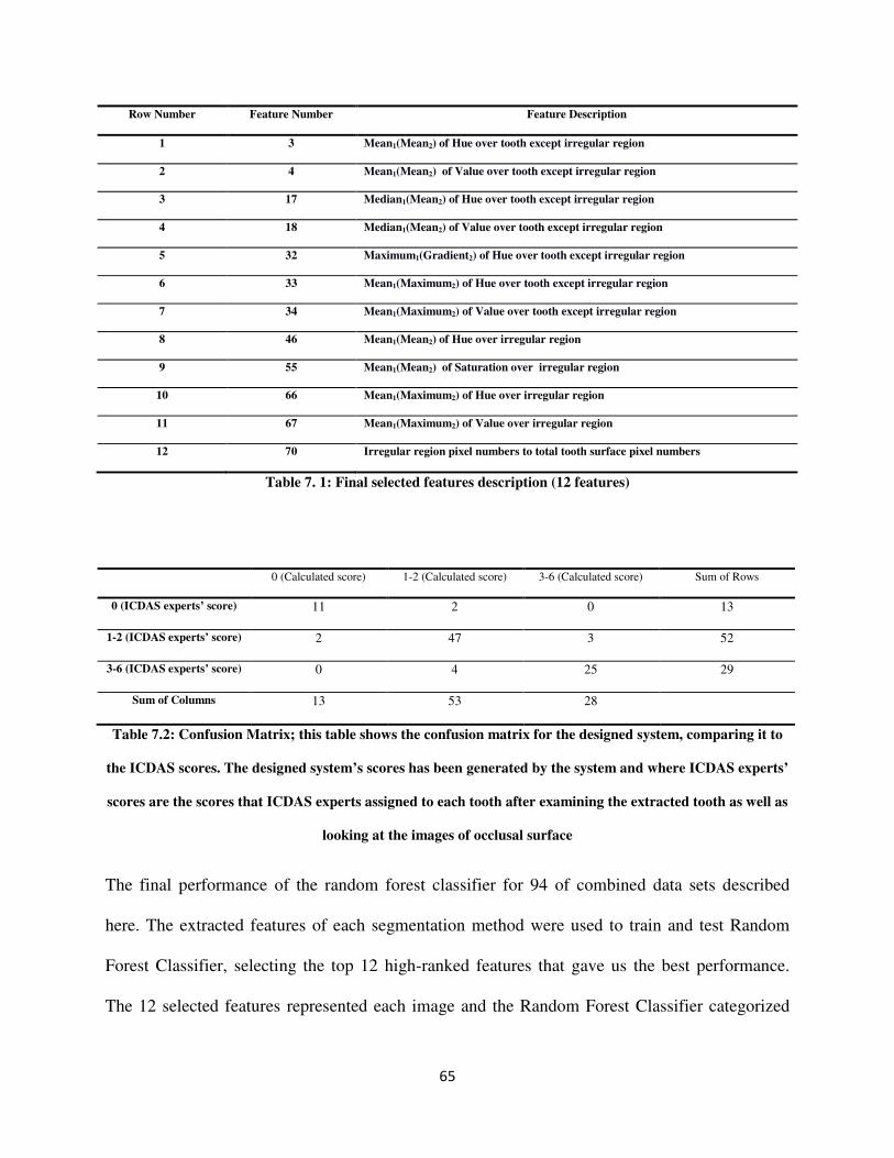
65

Row Number Feature Number Feature Description

1 3 Mean1(Mean2) of Hue over tooth except irregular region

2 4 Mean1(Mean2) of Value over tooth except irregular region

3 17 Median1(Mean2) of Hue over tooth except irregular region

4 18 Median1(Mean2) of Value over tooth except irregular region

5 32 Maximum1(Gradient2) of Hue over tooth except irregular region

6 33 Mean1(Maximum2) of Hue over tooth except irregular region

7 34 Mean1(Maximum2) of Value over tooth except irregular region

8 46 Mean1(Mean2) of Hue over irregular region

9 55 Mean1(Mean2) of Saturation over irregular region

10 66 Mean1(Maximum2) of Hue over irregular region

11 67 Mean1(Maximum2) of Value over irregular region

12 70 Irregular region pixel numbers to total tooth surface pixel numbers

Table 7. 1: Final selected features description (12 features)

0 (Calculated score) 1-2 (Calculated score) 3-6 (Calculated score) Sum of Rows

0 (ICDAS experts’ score) 11 2 0 13

1-2 (ICDAS experts’ score) 2 47 3 52

3-6 (ICDAS experts’ score) 0 4 25 29

Sum of Columns 13 53 28

Table 7.2: Confusion Matrix; this table shows the confusion matrix for the designed system, comparing it to

the ICDAS scores. The designed system’s scores has been generated by the system and where ICDAS experts’

scores are the scores that ICDAS experts assigned to each tooth after examining the extracted tooth as well as

looking at the images of occlusal surface

The final performance of the random forest classifier for 94 of combined data sets described

here. The extracted features of each segmentation method were used to train and test Random

Forest Classifier, selecting the top 12 high-ranked features that gave us the best performance.

The 12 selected features represented each image and the Random Forest Classifier categorized

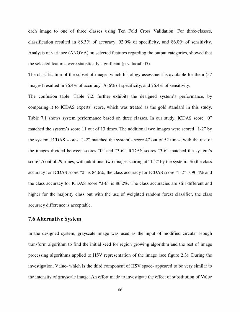
66

each image to one of three classes using Ten Fold Cross Validation. For three-classes,

classification resulted in 88.3% of accuracy, 92.0% of specificity, and 86.0% of sensitivity.

Analysis of variance (ANOVA) on selected features regarding the output categories, showed that

the selected features were statistically significant (p-value=0.05).

The classification of the subset of images which histology assessment is available for them (57

images) resulted in 76.4% of accuracy, 76.6% of specificity, and 76.4% of sensitivity.

The confusion table, Table 7.2, further exhibits the designed system’s performance, by

comparing it to ICDAS experts’ score, which was treated as the gold standard in this study.

Table 7.1 shows system performance based on three classes. In our study, ICDAS score “0”

matched the system’s score 11 out of 13 times. The additional two images were scored “1-2” by

the system. ICDAS scores “1-2” matched the system’s score 47 out of 52 times, with the rest of

the images divided between scores “0” and “3-6”. ICDAS scores “3-6” matched the system’s

score 25 out of 29 times, with additional two images scoring at “1-2” by the system. So the class

accuracy for ICDAS score “0” is 84.6%, the class accuracy for ICDAS score “1-2” is 90.4% and

the class accuracy for ICDAS score “3-6” is 86.2%. The class accuracies are still different and

higher for the majority class but with the use of weighted random forest classifier, the class

accuracy difference is acceptable.

7.6 Alternative System

In the designed system, grayscale image was used as the input of modified circular Hough

transform algorithm to find the initial seed for region growing algorithm and the rest of image

processing algorithms applied to HSV representation of the image (see figure 2.3). During the

investigation, Value- which is the third component of HSV space- appeared to be very similar to

the intensity of grayscale image. An effort made to investigate the effect of substitution of Value

67

in HSV space instead of intensity of the grayscale image. The alternative system would not

significantly change the performance of the classifier nor the time complexity of the

segmentation. The alternative system just reduces space complexity and can be considered as a

solution in case space complexity is important for the application.

Figure 7.22: Diagram of the alternative system components

68

Chapter 8

Summary and Future Work

8.1 Summary

In this work, an automated system to detect and score caries lesions on a set of in-vitro and in-

vivo images is developed and tested. An automated, user friendly system that eliminates the need

for manual land-marking while using advanced feature extraction methods leading to a more

reliable system for detection of early caries lesions has been developed. Two and three classes of

caries conditions were observed and compared.

The designed system may provide an advantage over existing systems, which require expensive

imaging sensors and external hardware. Another study which assessed performance of laser

fluorescence device (LF) and LF pen and Fluorescence camera (FC) in detecting occlusal caries

(Carious versus Non-Carious) by using histological gold standard described specificity and

sensitivity levels of 100% and 85% for LF, 80% and 89% for LF pen, 80% and 74% for FC

respectively [11], these are comparable to specificity and sensitivity of 88.3% and 86.0% in this

study when classifying to three classes. The system’s performance is better than LF pen and FC

and almost similar to LF.

Other existing technologies for caries diagnosis include devices based on laser fluorescence (LF

device, LF pen, F camera) or infrared (IR) laser fluorescence, referred to as quantitative laser or

light fluorescence (QLF). Electrical conductance measurements (ECM), direct digital

69

radiography, Digital Imaging Fiber-Optic Trans-Illumination (DIFOTI) and simple Fiber Optic

Trans-Illumination (FOTI), LED-based caries detector and less popular fluorescence

spectrophotometer, MicroCT and heat induced detection technique [3, 7-12]. Data show varying

degrees of sensitivity and specificity for In-Vitro and In-Vivo studies [3, 8-9, 13-15]. In addition

to the unpredictable accuracy and the relatively high price, the existing technologies are user

sensitive and require several steps in order to perform a clinical reading correctly. The value

given by these caries detection devices is subjectively interpreted by the clinician and thus

requires a trained dental professional to make a diagnostic or treatment decision.

Relatively easy-to-use, widely available and inexpensive hardware imaging techniques, such as

an intraoral camera, may easily augment the decision making process of treatment provided to

patients (surgical or preventive) and their overall impression of dental care they are receiving.

The use of computer-aided systems to detect caries lesions based on different types of tooth

images may be a way to increase the sensitivity of caries detection. There is promising evidence

that the automated caries detection system using intraoral photographs can provide high

sensitivity and specificity rates when compared with ICDAS scores [39].

8.2 Future Work

The future work of this dissertation is as follows.

� Evaluation of the method on a larger in-vitro data set, following with the histological

assessment of caries.

� Evaluation of the method for a larger in-vivo data set.

70

Bibliography

[1] http://www.who.int/mediacentre/factsheets/fs318/en/

[2] Caries Annual Report - NIDCR/CDC Dental, Oral and Craniofacial Data Resource Center

(DRC), http://drc.hhs.gov/report/1_3.htm accessed on 8/29/13.

[3] A.F. Zandona, D.T. Zero, Diagnostic tools for early caries detection, The Journal of the

American Dental Association 137 (12) (2006) 1675-1684.

[4] M. Toraman Alkurt, I. Peker, H. Deniz Arishu, O. Bala, B. Altunkaynak, In-Vivo

comparison of laser fluorescence measurements with conventional methods for occlusal

caries detection, Lasers in medical science 23 (3) (2008) 307-312.

[5] A.I. Ismail, Visual and Visuo-tactile Detection of Dental Caries, Journal of Dental Research

83 (2004) C56-C66.

[6] B. Senel, K. Kamburoglu, O. Ucok, S.P. Yuksel, T. Ozen , H. Avsever, Diagnostic accuracy

of different imaging modalities in detection of proximal caries, Dentomaxillofacialradiology

39 (8) (2010) 501-511.

[7] G.K. Rochlen , M.S. Wolff, Technological advances in caries diagnosis, Dental clinics of

North America 55 (3) (2011) 441-452.

[8] M.B. Diniz, T. Boldieri, J.A. Rodrigues, L. Santos-Pinto, A. Lussi, R.C. Cordeiro, The

performance of conventional and fluorescence-based methods for occlusal caries detection:

an In-Vivo study with histologic validation, Journal of the American Dental Association 143

(4) (2012) 339-350.

71

[9] J.H. Berg, E.J Swift, Current caries detection devices, Journal of Esthetic and Restorative

Dentistry 22 (5) (2010) 464-470.

[10] L. Duruturk, A. Ciftci, S. Baharoglu, D. Oztuna, Clinical evaluation of DIAGNOdent in

detection of occlusal caries in newly erupted noncavitated first permanent molars in caries-

active children, Operative Dentistry 36 (4) (2011) 348-355.

[11] M. Graye, K. Markowitz, M. Strickland, G. Guzy, M. Burke, M. Houpt, In-Vitro

evaluation of the Spectra early caries detection system, The Journal of clinical dentistry 23

(1) (2012) 1-6.

[12] O. Samek, H.H. Telle, D.C.S. Beddows, Laser-induced breakdown spectroscopy: a tool

for real-time, In-Vitro and In-Vivo identification of carious teeth, BMC Oral Health 1 (2001)

1-1.

[13] A.M. Aktan, M.A. Cebe, M.E. Ciftci, E.S. Karaarslan, A novel LED-based device for

occlusal caries detection, Lasers in Medical Science. 27 (2012) 1-7.

[14] A. Jablonski-Momeni, D.N. Ricketts, S. Rolfsen, R. Stoll, M. Heinzel-Gutenbrunner, V.

Stachniss, K. Pieper, Performance of laser fluorescence at tooth surface and histological

section, Lasers in Medical Science 26 (2) (2011) 171-178.

[15] K.W. Neuhaus, C. Longbottom, R. Ellwood, A. Lussi, Novel lesion detection aids,

Monographs in oral science 21 (2009) 52-62.

[16] V. Baelum, H. Hintze, A. Wenzel, B. Danielsen, B. Nyvad, Implications of caries

diagnostic strategies for clinical management decisions, Community Dentistry and Oral

Epidemiology 40 (3) (2012) 257-266.

72

[17] International Caries Detection and Assessment System (ICDAS) Coordinating

Committee, Criteria Manual International Caries Detection and Assessment System (ICDAS

II), (2009).

[18] A.I. Ismail, W. Sohn, M. Tellez, A. Amaya, A. Sen, H. Hasson, N.B. Pitts, The

International Caries Detection and Assessment System (ICDAS): an integrated system for

measuring dental caries, Community Dentistry and Oral Epidemiology 35 (3) (2007) 170-

178.

[19] A. Jablonski-Momeni, V. Stachniss, D.N. Ricketts, M. Heinzel-Gutenbrunner, K. Pieper,

Reproducibility and accuracy of the ICDAS-II for detection of occlusal caries In-Vitro,

Caries Research 42 (2) (2008) 79-87.

[20] M.M. Braga, M.S. de Benedetto, J.C. Imparato, F.M. Mendes, New methodology to

assess activity status of occlusal caries in primary teeth using laser fluorescence device,

Journal of Biomedical Optics 15 (4) (2010) 047005.

[21] 40J.A. Rodrigues, K.W. Neuhaus, M.B. Diniz, I. Hug, H. Stich, L. Karlsson, A. Lussi,

Comparison among gold standard techniques used for the validation of methods for occlusal

caries detection, Microscopyresearch andtechnique 75 (5) (2012) 605-608.

[22] http://faculty.mu.edu.sa/public/uploads/1380556025.9751The%20tooth%20supporting%

20structures.pdf

[23] D. L. Pham, C. Xu, and J. L. Prince. Current Methods in Medical Image Segmentation.

Annu. Rev. Biomed. Eng.,315-337, 2000.

[24] Z. Ma, J. M. Tavares, R. N. Jorge, and T. Mascarenhas. A review of algorithms for

medical image segmentation and their applications to the female pelvic cavity. Comput

Methods Biomech Biomed Engin.235-46, 2010.

73

[25] N. Otsu. A Threshold selection method from gray-level histograms. IEEE Trans. On

Systems, Man, and Cybernetics, 9(1): 62-66, 1979.

[26] M. Sezgin. Survey over image thresholding techniques and quantitative performance

evaluation. Journal of Electronic Imaging, 2004.

[27] S. Wang, F. Chung, and F. Xiong. A novel image thresholding method based on parzen

window estimate. Pattern Recognition, 41: 117-129, 2008.

[28] M. Maitra and A. Chatterjee. A hybrid cooperative comprehensive learning based PSO

algorithm for image segmentation using multilevel thresholding. Expert Systems with

Applications, 34(2): 1341-1350, 2008.

[29] K. Hammouche, M. Diaf, and P. Siarry. A multilevel automatic thresholding method

based on genetic algorithm for fast image segmentation. Computer Vision and Image

Understanding, 109: 163-175, 2008.

[30] D. Y. Kim and J. W. Park. Connectivity-based local adaptive thresholding for carotid

artery segmentation using MRA images. Image and Vision Computing, 23(14):1277-1287,

2005.

[31] O. P. Verma, M. Hanmandlu, S. Susan, M. Kulkarni and P. Kumar. A Single Seeded

Region Growing Algorithm for Color Image Segmentation Using Adaptive Thresholding.

IEEE International Conference on Communication Systems and Network Technologies.

500-503, 2011.

[32] M. Kass, A. Witkin and D. Terzopoulos. Snakes: Active contour models. International

Journal of Computer Vision. (1) 321-331, 1988.

74

[33] E. A. Gehan. A generalized Wilcoxon test for comparing arbitrarily singly-censored

samples. Biometrika 52(1) 203-223, 1965.

[34] H. D. Cheng, X.H. Jiang, Y. Sun and J. Wang. Color image Segmentation: advances and

prospects. Pattern Recognition 34(12) 2259-2281, 2001.

[35] http://en.wikipedia.org/wiki/HSL_and_HSV

[36] S. Dreiseutl, L. Ohno-Machado, Logistic regression and artificial neural network

classification models: a methodology review, Journal of Biomedical Informatics 35(5)

(2002) 352-359.

[37] L. Breiman, Random Forests, Machine Learning 45 (2001) 5-32.

[38] I. Guyon, J. Weston, S. Barnhill, and V. Vapnik. Gene selection for cancer classification

using support vector machines. Machine Learning, 46:389–422, 2002.

[39] R. C. Gonzalez and R. E. Woods. Digital Image Processing, 2008.

[40] R.O. Duda, P.E. Hart, Use of the Hough Transformation to Detect Lines and Curves in

Pictures, Communication of the ACM 15 (1) (1972) 11-15.

[41] M. Rizon, H. Yazid, P. Saad, A.Y.M. Shakaff, A.R. Saad, S. Masanori, S. Yaccob, M.R.

Mamat, M. Karthigayan, Object detection Using Circular Hough Transform, American

Journal of Applied Sciences 2 (12) (2005) 1606-1609.

[42] I. Daubechies, Ten lectures on wavelets, CBMS-NSF conference series in applied

mathematics, SIAM Ed (1992).

[43] A.I. Ismail, M. Tellez, N.B. Pitts, K.R. Ekstrand, D. Ricketts, C. Longbottom, H.

Eggertsson, C. Deery, J. Fisher, D.A. Young, J.D.B. Featherstone, R.W. Evans, GG. Zeller,

D. Zero, S. Martignon, M. Fontana, A. Zandona, Caries management pathways preserve

dental tissues and promote oral health, Community Dent Oral Epidemiol 41 (2013) e12–e40.

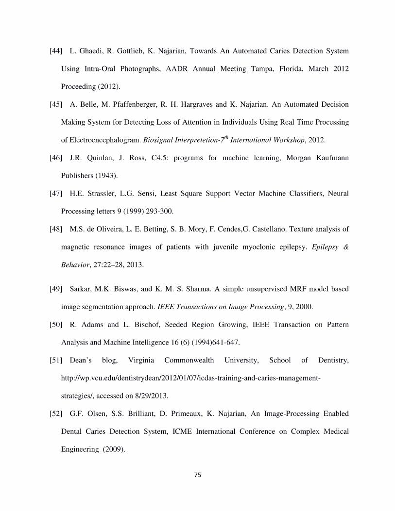
75

[44] L. Ghaedi, R. Gottlieb, K. Najarian, Towards An Automated Caries Detection System

Using Intra-Oral Photographs, AADR Annual Meeting Tampa, Florida, March 2012

Proceeding (2012).

[45] A. Belle, M. Pfaffenberger, R. H. Hargraves and K. Najarian. An Automated Decision

Making System for Detecting Loss of Attention in Individuals Using Real Time Processing

of Electroencephalogram. Biosignal Interpretetion-7th

International Workshop, 2012.

[46] J.R. Quinlan, J. Ross, C4.5: programs for machine learning, Morgan Kaufmann

Publishers (1943).

[47] H.E. Strassler, L.G. Sensi, Least Square Support Vector Machine Classifiers, Neural

Processing letters 9 (1999) 293-300.

[48] M.S. de Oliveira, L. E. Betting, S. B. Mory, F. Cendes,G. Castellano. Texture analysis of

magnetic resonance images of patients with juvenile myoclonic epilepsy. Epilepsy &

Behavior, 27:22–28, 2013.

[49] Sarkar, M.K. Biswas, and K. M. S. Sharma. A simple unsupervised MRF model based

image segmentation approach. IEEE Transactions on Image Processing, 9, 2000.

[50] R. Adams and L. Bischof, Seeded Region Growing, IEEE Transaction on Pattern

Analysis and Machine Intelligence 16 (6) (1994)641-647.

[51] Dean’s blog, Virginia Commonwealth University, School of Dentistry,

http://wp.vcu.edu/dentistrydean/2012/01/07/icdas-training-and-caries-management-

strategies/, accessed on 8/29/2013.

[52] G.F. Olsen, S.S. Brilliant, D. Primeaux, K. Najarian, An Image-Processing Enabled

Dental Caries Detection System, ICME International Conference on Complex Medical

Engineering (2009).

76

[53] C. Huang, Q. Liu and X. Li. Color Image Segmentation by Seeded Region Growing and

Region Merging. IEEE Seventh International conference on Fuzzy Systems and Knowledge

Discovery. 533-536, 2010.

[54] J. M. Pardo, D. Cabello and J. Heras. A snake for model-based segmentation of

biomedical images. Pattern Recognition Letters. (18) 1529-1538, 1997.

[55] http://www.eurekafamilydental.com/services/oral-exams-x-rays/

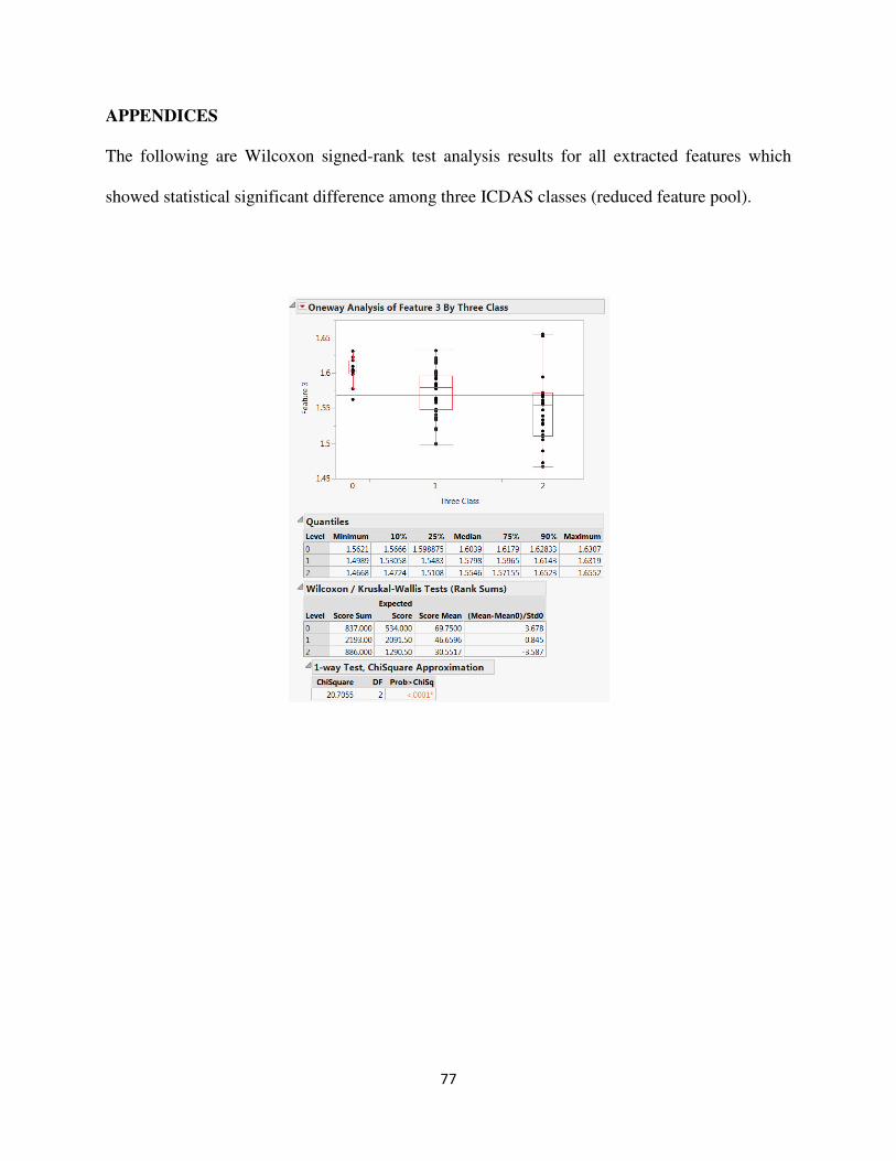
77

APPENDICES

The following are Wilcoxon signed-rank test analysis results for all extracted features which

showed statistical significant difference among three ICDAS classes (reduced feature pool).

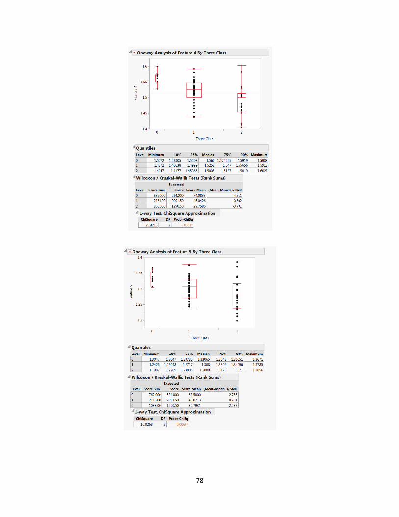
78

79

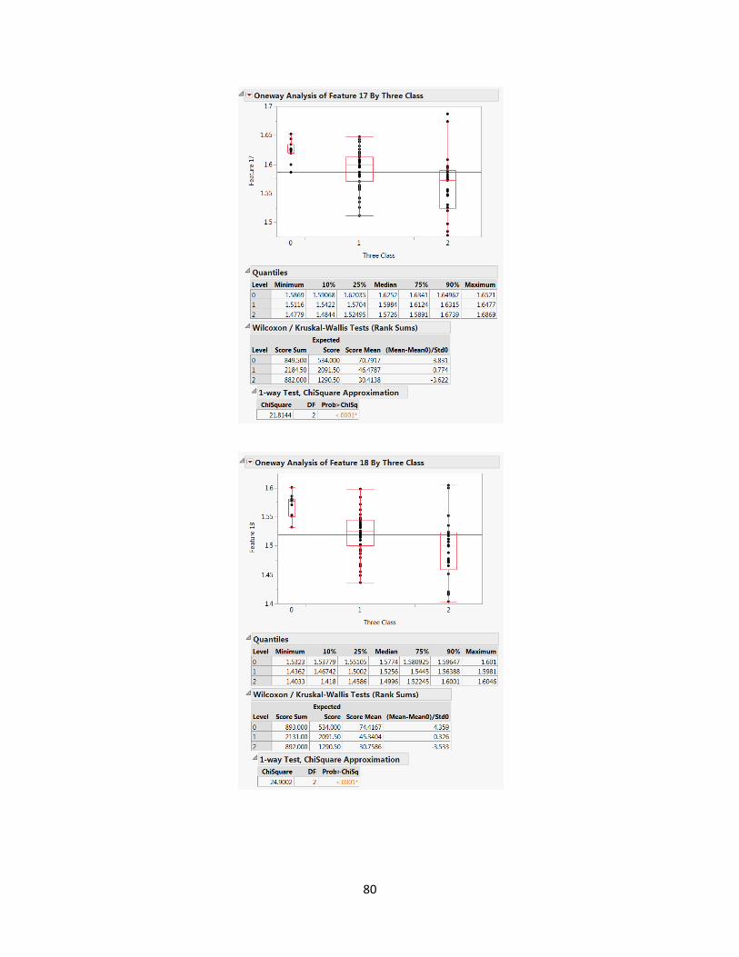
80

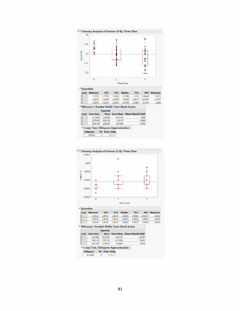
81

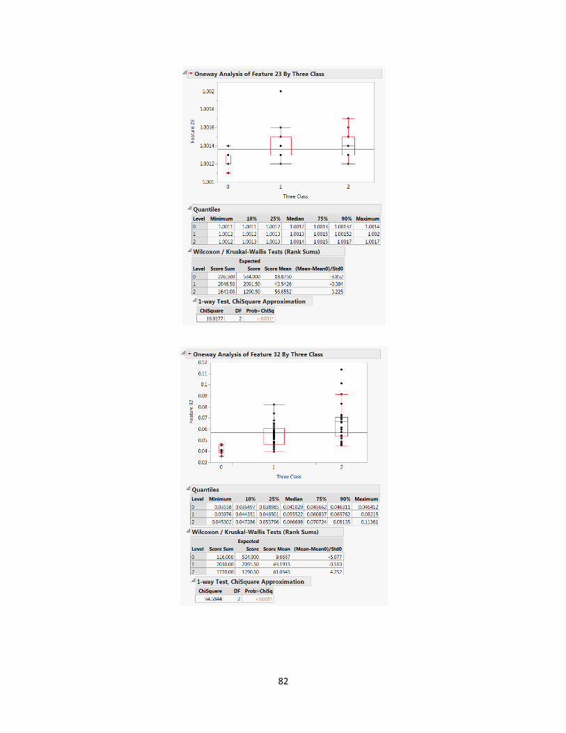
82

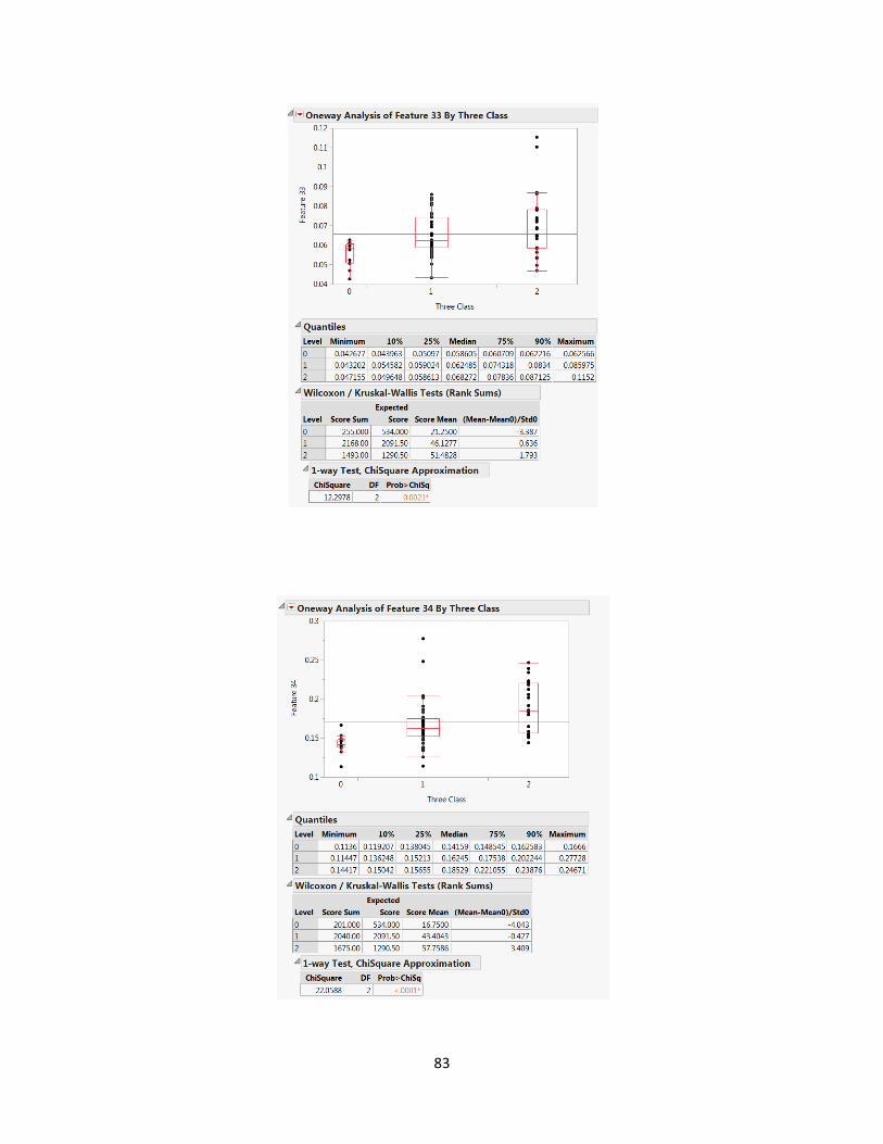
83

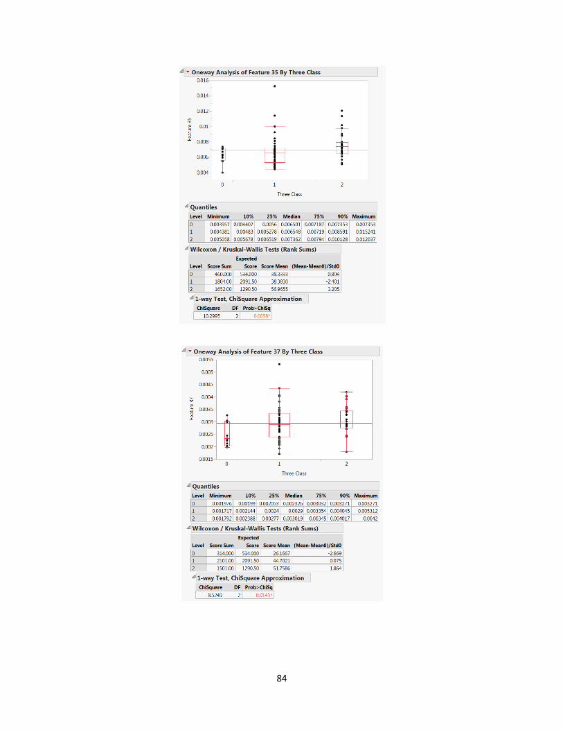
84

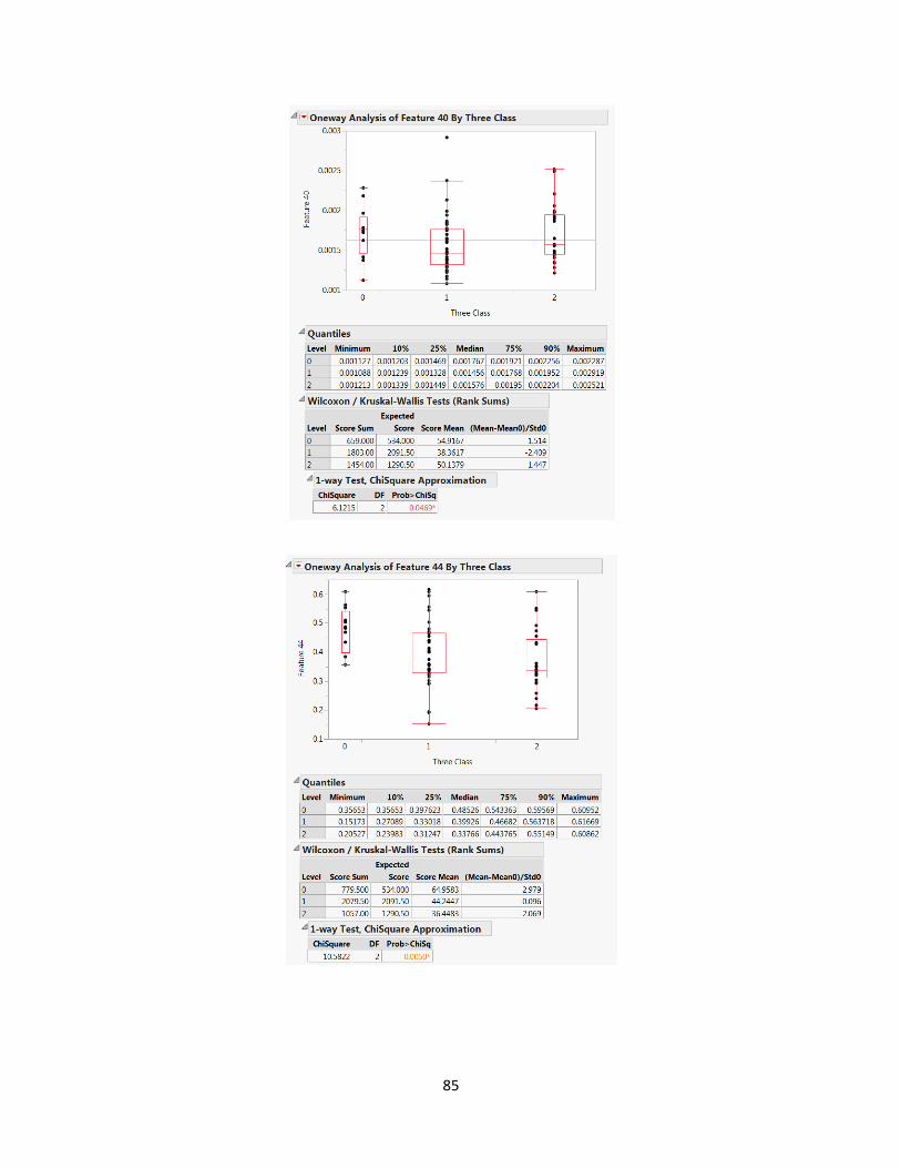
85

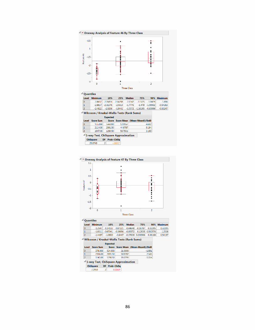
86

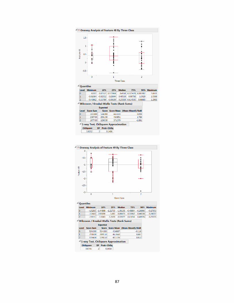
87

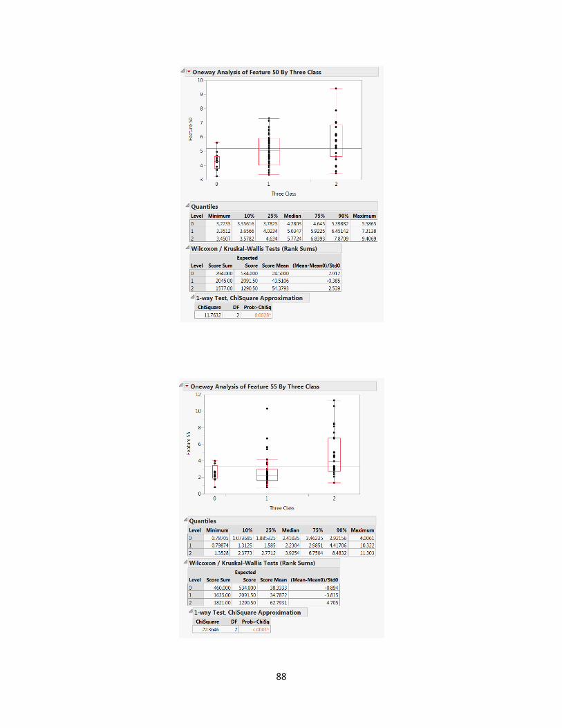
88

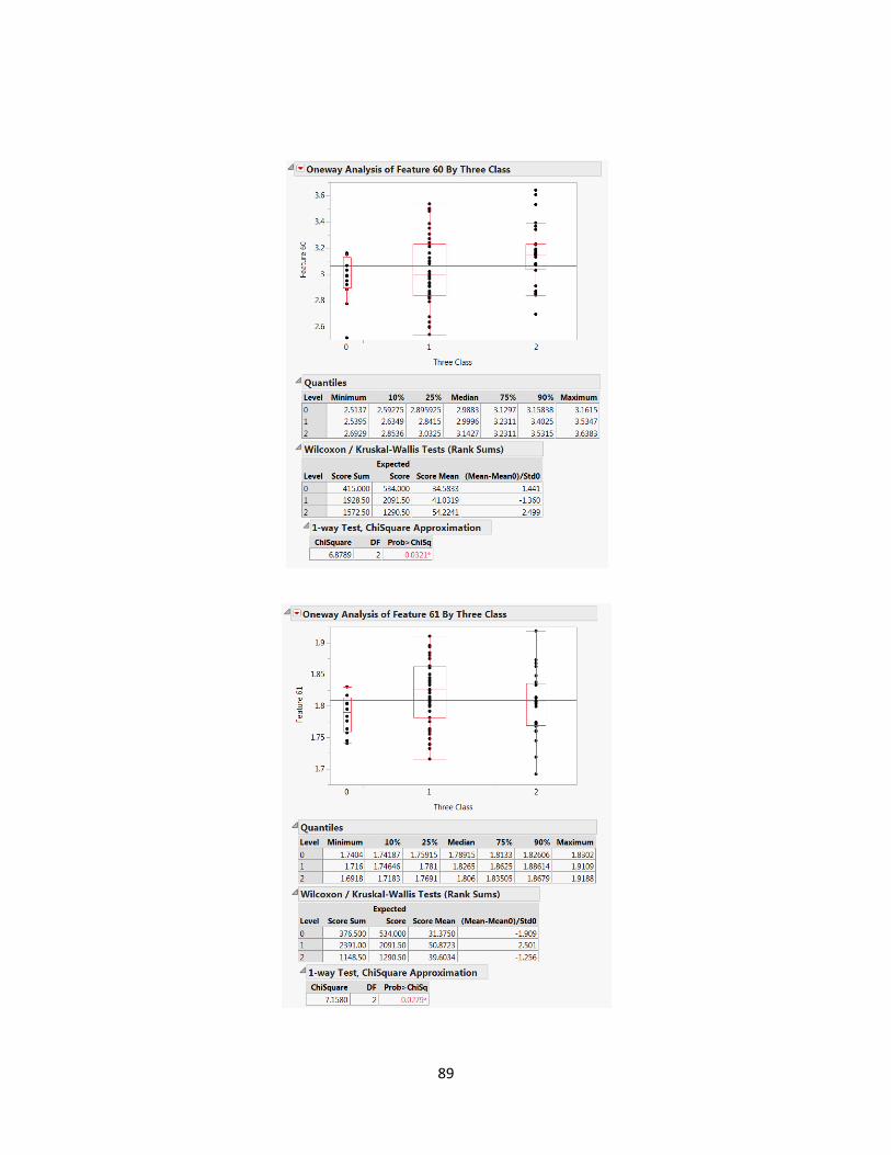
89

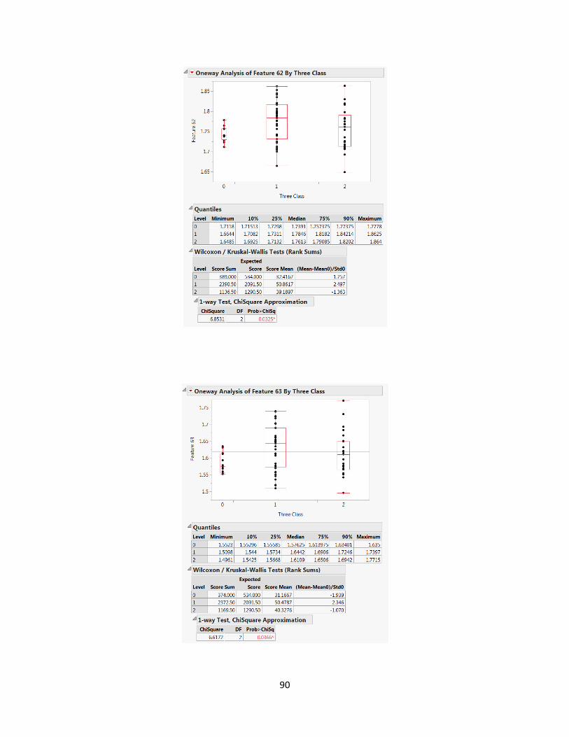
90

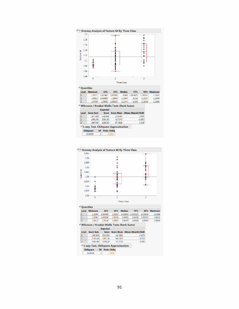
91

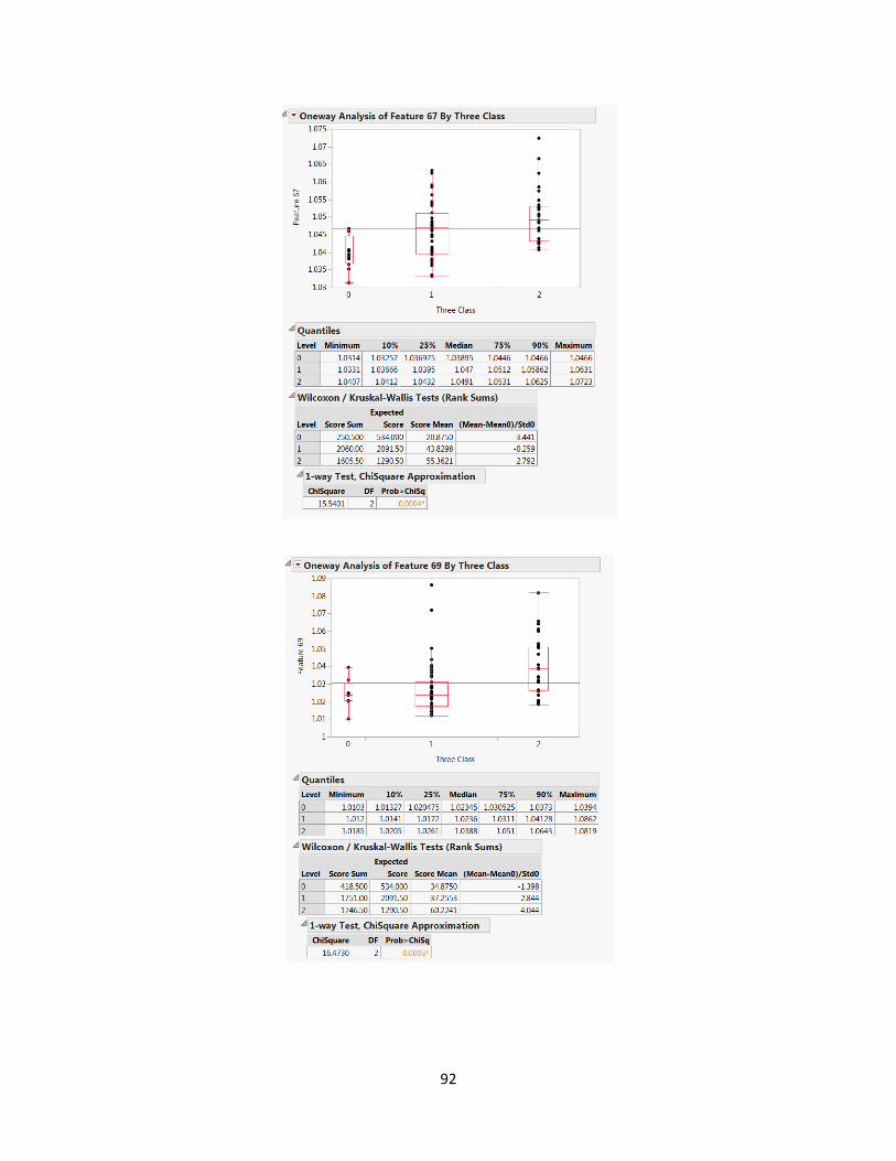
92

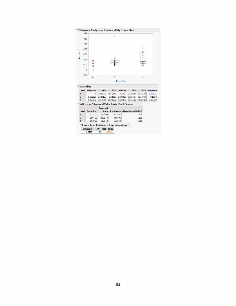
93