PANG Pak Long Year 1, Dual Degree Program in Technology and Management Supervised by: Professor David ROSSITER Department of Computer Science and Engineering COMP 4971C - INDEPENDENT WORK (SPRING 2018/19) A STUDY TO DETERMINE OBJECTIVE TRADING SIGNALS FROM SIMPLE MOVING AVERAGES USING AN INNOVATIVE STRATEGY

Welcome message from author
This document is posted to help you gain knowledge. Please leave a comment to let me know what you think about it! Share it to your friends and learn new things together.
Transcript

Pang Pak Long (20536988)
PANG Pak Long Year 1, Dual Degree Program in Technology and Management Supervised by: Professor David ROSSITER Department of Computer Science and Engineering
COMP 4971C - INDEPENDENT WORK (SPRING 2018/19)
A STUDY TO DETERMINE OBJECTIVE TRADING SIGNALS FROM SIMPLE MOVING AVERAGES
USING AN INNOVATIVE STRATEGY

1
Contents
Abstract .............................................................................................................................. 3
Introduction ........................................................................................................................ 3
Research Question ............................................................................................................. 4
Aim ................................................................................................................................ 4
Hypothesis ..................................................................................................................... 4
Methodology ...................................................................................................................... 4
Tools Used in This Project ............................................................................................. 4
The Methodology of Evaluating a Strategy ................................................................... 5
How Backtest is Performed ........................................................................................... 5
Choice of Indicators ....................................................................................................... 6
Development ...................................................................................................................... 7
Preliminary Research on Crossing between SMAs ....................................................... 7
Further Research on Possible Indicators ...................................................................... 11
An Attempt to Add Long-term SMA as an Additional Indicator ................................ 13
An Attempt to Use the Concept of Parallel SMA as Indicators .................................. 15
Results .............................................................................................................................. 17
Results of the Final Strategy ........................................................................................ 17
Results of Other Groups of SMAs ............................................................................... 21
Results of Trading in Foreign Market .......................................................................... 22
Conclusion ....................................................................................................................... 25
Evaluation and Further Developments............................................................................. 26
Appendix .......................................................................................................................... 27
Appendix 1: Sample HTML Report from Backtesting of the Final Strategy .............. 27
Appendix 2: The Results of the Final Strategy Trading in the Hang Seng Index ....... 29

2
Tables of Figures
Figure 1: Flowchart for stoxy backtesting ......................................................................... 5
Figure 2: An example of SMAs crossing ........................................................................... 6
Figure 3: SMA 10 & 20 Cross Up Boxplot ....................................................................... 7
Figure 4: SMA 10 & 20 Cross Up Raw Data .................................................................... 7
Figure 5: SMA 10 & 20 Cross Down Boxplot .................................................................. 8
Figure 6: SMA 10 & 20 Cross Down Raw Data ............................................................... 8
Figure 7: Backtest for Trading with Simple Crossing ....................................................... 8
Figure 8: SMA 100 & 250 Cross Up Boxplot ................................................................... 9
Figure 9: SMA 100 & 250 Cross Up Raw Data ................................................................ 9
Figure 10: SMA 100 & 250 Cross Down Boxplot .......................................................... 10
Figure 11: SMA 100 & 250 Cross Down Raw Data ....................................................... 10
Figure 12: An Example of the Start of an Upward Trend ............................................... 11
Figure 13: An Example of the End of an Upward Trend ................................................. 12
Figure 14: Result of Backtest with Long-term Checking ................................................ 13
Figure 15: The Change in Total Worth for Using Long-term Checking ......................... 14
Figure 16: Result of Parallel Checking ............................................................................ 15
Figure 17: Results of Backtest with Parallel Checking ................................................... 16
Figure 18: Flowchart for the Final Strategy ..................................................................... 17
Figure 19: Results of Backtest using the Final Strategy .................................................. 18
Figure 20: The Change in Total Worth for Using the Final Strategy .............................. 19
Figure 21: CAGR of The Final Strategy .......................................................................... 20
Figure 22: Gain Against the Number of Days Holding using the Final Strategy ............ 20
Figure 23: The Change in Total Worth for Trading in the S&P 500 ............................... 23
Figure 24: CAGR for Trading in the S&P 500 ................................................................ 23
Figure 25: Percentage Gain Against the Number of Days in the S&P 500 ..................... 24
Table of Tables
Table 1: Result of Trading with Simple Crossing ............................................................. 9
Table 2: Results of Backtest with Long-term Checking .................................................. 14
Table 3: Results of Trading with Final Strategy using SMA 10, 20 and 50 .................... 19
Table 4: Results of the Final Strategy with Different Combinations of SMA ................ 21
Table 5: Results of the Final Strategy in Foreign Indexes ............................................... 22
Table 6: Full Results of the Final Strategy with Different Combinations of SMA ......... 29

3
Abstract
Moving average is a common and simple tool for trend analysis in the stock market. This
project creates an innovative, yet objective strategy to predict and provide a trading signal to
maximize the profit. A computer program is utilized to do multiple backtesting to optimize the
parameters with objective references like the compound annual growth rate. By creating
indicators like checking if the two simple moving averages are “parallel” or checking the
percentage differences between price and long-term moving averages, the strategy takes
multiple indicators’ results into account. It provides a buy or a sell signal with some logic
checks between multiple indicators.
This project is able to increase the compound annual growth rate after adding multiple
indicators for checking into the strategy. After applying the strategy, the number of trades
during the backtesting is lower while the number of days holding the stocks increases, with a
significant increase in the percentage gain for each trade. The strategy is tested and perform
successfully in the Hang Seng Index and other foreign indexes, like the S&P 500, CAC 40 and
Nikkei 225.
Introduction
This project focuses on analysing and optimizing indicators using simple moving averages
(SMAs). SMAs are the averages of the price in a certain past period of time. For example, SMA
10 means the average of the past 10 days price. SMAs are simple and easy to understand, which
are always displayed along with the price on the stock price chart. It is a common tool for trend
analysis.
However, mature traders in the market seldom solely rely on moving averages to be the
indicators for trading signals, mainly due to two reason. First, SMAs are always delayed in
time as they are calculated based on past data. In which case, SMA always only gives a
confirmation of the trend instead of predicting the trend. Second, when the market price is
choppy, moving averages often give unreliable information as they are incapable to provide
information on short-term fluctuations.
Another potential problem when buyers use moving average is, they may take the moving
average as a resistance or support level with subjective thoughts. They may adjust their choice
of parameters, like the number of days to average, to fit their idea, which leads to an unreliable
conclusion and hence bad decision making.
Therefore, this project tries to find and optimize new methods to predict the trend using
SMAs.

4
Research Question
A Study to Determine Objective Trading Signals from Simple Moving Averages Using an
Innovative Strategy
Aim
This project aims to provide a method of trading in the stock market by optimizing the
parameters of different indicators using moving averages. By using the combinations of three
SMAs signals, this project aims to identify a trend right after it started, before it grows. The
signals and indicators provided in this project are aimed to give an objective conclusion based
on multiple backtesting. Also, this project aims to find the possibility of innovative, yet
objective ways to use SMA for predicting the trend and optimizing parameters for trading.
Hypothesis
This project would like to predict the trend right after it starts using the combination of
SMAs. In the view of using combinations of SMA, this gives extra information compared to
relying on only one SMA solely. For example, calculating the change in the difference between
SMAs may help to identify signals for possible upward or downward trend. Therefore, this
project would like to test if combinations of SMA will be better than using a single SMA. Is
using combinations a better strategy for getting trading signals from SMA?
If a group of SMAs is used, both short-term information and long-term information should
be considered. Short-term information is the fluctuation and the latest trending of the price,
with less time delay, while the long-term information is the long-term trending the stock is
going. Two short-term SMAs crossing should be information for short-term price changing
while one more long-term SMA should be added for comparison to get long-term trending
information. By comparing the two information, the strategy should be able to predict the
coming long-term trend.
Methodology
Tools Used in This Project
This project will develop algorithms to do backtest to optimize parameters and test out the
effectiveness of indicators, where large amounts of data will be used and generated during
backtesting. Therefore, this project selects Python as the language for its simple syntax and
easy implementation. Also, Python has a lot of open source libraries like pandas and matplotlib
for dealing with large amounts of data, which can simplify the development progress. All the
source code in this program is developed on a program called Stoxy, kindly provided by Prof.
David Rossiter, the supervisor of this project. Last but not least, the source of data in this project
is from Yahoo Finance, where these historical data are downloaded and imported into Stoxy
for further processing and backtesting.

5
The Methodology of Evaluating a Strategy
This project would like to focus on the Hong Kong stock market as the base for developing
the trading strategy. As such, the Hang Seng Index is selected for all the backtesting and
demonstrations. Backtest will be conducted starting from the date the Hang Seng Index is
released, 31st December 1986, to the current date, 29th April 2019.
The successfulness of a strategy is evaluated by the worth it can generate from it. Worth
is calculated by backtesting using algorithms. The system starts with 1 million dollars and it
will buy as much stock as it can on every buy signal while selling all its holding stock when
there is a sell signal. The worth is defined as the sum of cash on hand and the total value of the
holding stocks.
Compound annual growth rate (CAGR) is used to evaluate the average annual return of
the strategy, as the calculated worth is a geometric progression. CAGR provides a constant rate
of return of the worth from the beginning balance to the ending balance, even the worth in this
project is a geometric progression. This provides a proper evaluation and comparison between
different strategy. The formula of CAGR is stated as follows, where n is the number of years.
To calculate the annual change, CAGR is used with n (the number of years) set to one.
𝐶𝐴𝐺𝑅 = 𝐸𝑛𝑑𝑖𝑛𝑔 𝐵𝑎𝑙𝑎𝑛𝑐𝑒
𝐵𝑒𝑔𝑖𝑛𝑛𝑖𝑛𝑔 𝐵𝑎𝑙𝑎𝑛𝑐𝑒
1𝑛
− 1
How Backtest is Performed
Figure 1 is a flowchart that indicates how backtesting is done in stoxy. There are two main
features in this flow. First, it performs backtest for all the grouping combinations between
SMAs, and data are stored for later analysis. Second, the HTML report allows a simple
comparison between different strategy or different parameters.
Figure 1: Flowchart for stoxy backtesting

6
Choice of Indicators
The indicators in this project would like to only focus on the relationship between moving
averages and the price. To keep it simple, this project would like to also keep it with three
moving averages at most in the development and analysis process.
Initially, the combinations of three simple moving averages are designed as two being
short-term indicators and the last as the long-term indicator. The long-term SMA will act as a
base and indicates how the long-term trend is going, while two short-term SMAs giving
primary trading signals. By identifying the relationship between three SMA, it aims to provide
an objective strategy with both long-term and short-term information, result in less time
delayed and more reliable signals. As such, three moving averages would be good enough. If
one more moving average is added to the analysis, it will have too much information to process,
while removing one moving average will not be enough to predict the trend.
Different from SMA, there are exponential moving averages (EMAs). It is a weighted
moving average that weight more on recent price data than the past. This gives more updated
information for the moving average. However, the method of weighting can largely affect the
effectiveness of EMAs. Using EMA brings complexity to finding an innovative strategy.
Hence, the development of this project will only base on SMA. The final result may be able to
apply on EMAs, but the development process would be easier if based on SMAs only.
For selecting the number of days to average, this project would like to stick with the one
normally people use, like selecting among 5, 10, 20, 50, 100, 250. The reason behind is the
self-fulfilling prophecy of traders in the market. Since there is a large portion of traders in the
market looking at these common moving averages, their beliefs to these moving averages may
probably cause the expectations to come true, which is also a factor this project should consider
when analysing the behaviour of a stock. For example, as indicates as point A in Figure 2,
people believe 20-days moving average crossover 50-days moving average indicates an upward
trend. People may buy when it occurs and eventually the price would increase as the demand
increases. Therefore, this project would like to stick to use the moving averages that people
normally look at, to take factors like self-fulfilling into account.
Figure 2: An example of SMAs crossing
A
B

7
Development
Preliminary Research on Crossing between SMAs
SMA is defined as the average price of a past period of time n. For example, SMA 20
means n is 20 where SMA 20 on that day is the average of the price of the past 20 days. The
formula for nth days SMA value on the kth day is stated follows:
𝑆𝑀𝐴 𝑛𝑘 = 1
𝑛∑ 𝑃𝑖
𝑘
𝑖=𝑘−𝑛+1
The crossing of SMAs is always used as an indicator for possible upward or downward
trends. In general implementation, a short-term SMA cross from below long-term SMA to
above SMA is called crossing up, like point A in Figure 2. On the other hand, short-term SMA
cross from above to below the long-term SMA is called crossing down, like point B in Figure
2. When crossing up occurs, meaning the price increase significantly compared to the long-
term trend in the past. Same as the crossing down situation, it means the price drops
significantly in the short-term. Therefore, people believe crossing up implies an increase in
price in the future while crossing down implies a decrease in price in the future.
This project would like to verify this belief. The program loop from the starting date of
the stock releases to the current date as the ending date. Multiple inputs can be taken and
comparison between every pair is conducted. For example, SMA 10, 20, 50 and 100 is inputted
to the program, six possible pairs are compared, which include 10 and 20, 10 and 50, 10 and
100, 20 and 50, etc.
The change in the price of 150 days after every cross up and cross down is recorded. The
following show the change in the price of every 10 and 20 crosses up of the Hang Seng Index
for checking from 31st December 1986 to 29th April 2019.
There is a lot of cases that SMA 10 and SMA 20 crosses. Figure 4 shows all the data
points of the change in price after cross up occurs. Figure 3 is a box plot diagram is plotted to
show the general price change after crossing up. The orange line in the box is the median and
the green line is the average of the data. The crosses outside the bars are the outliers in the data
set.
Figure 4: SMA 10 & 20 Cross Up Raw Data Figure 3: SMA 10 & 20 Cross Up Boxplot

8
Similarly, the same testing is done to all cross down. The result is shown below.
From this result, it shows that the price generally increases after crossing up. However,
the trend is not significant where there are still a significant amount of cases having the price
decreases after crossing up. For cross down, the price seems to decrease at the beginning but
start to increase back after a month. In which case, crossing down does not really show a
possible downward trend.
A backtest is done for these two SMAs to find the worth and the CAGR. It buys as much
as it can when it crosses up and sells all stock when it crosses down.
The result is shown in Figure 7. The buy signal is labelled as “BUY” and the sell signal is
labelled as “SELL”. The blue line shows the change in worth over time. However, the result is
as good as expected. Table 1 summarizes the result of worth and the CAGR of worth.
Figure 7: Backtest for Trading with Simple Crossing
Figure 6: SMA 10 & 20 Cross Down Raw Data Figure 5: SMA 10 & 20 Cross Down Boxplot

9
Table 1: Result of Trading with Simple Crossing
SMA 10 and 20 Total Worth (%) CAGR (%)
Buy and Hold 1052.7 7.85
Trade without checking 580.9 6.11
The total worth and the CAGR are both lower than just buy and hold at the beginning,
which is not desired. The signal cannot identify the upward trend and downward trend, but just
trading randomly. The change in price after the crossing is distributed randomly as shown in
the above boxplot diagrams.
In fact, taking this result as an example, the result is restricted with the data set input. The
Hang Seng Index has up cycles and down cycles, but it is increasing in the long-term, starting
from 1986 till 2019. Hence, on average in long-term trading in with the Hang Seng Index will
probably gain, but this does not mean that crossing up can successfully predict an upward trend.
The crossing between SMA 100 and 250 also clearly show how long-term economic growth
affects the change of price after crossing.
With fewer crosses occurs between SMA 100 and 250, it clearly shows that after crossing
up the price tends to increase in the long-term. However, it is the same with crossing down, as
shown in Figure 10, the change in price distribute normally and slightly increasing even after
crossing down.
Figure 9: SMA 100 & 250 Cross Up Raw Data Figure 8: SMA 100 & 250 Cross Up Boxplot

10
By this, using the crossing of moving averages is not a good indicator for trending as it
cannot predict the future trend of the price accurately. Instead, the filter should be used to check
whether the crossing up is indicating an increase in an upward trend and crossing down is
actually coming with a downward trend.
A filter should be used to check for the crossing signal. As shown in Figure 7, the buy and
sell signals are triggered multiple times during both the upward trend and downward trend.
This leads to a reduced gain in the upward trend and a loss in the downward trend, which is not
a desired situation for a trading strategy. Therefore, filter to limit the number of trades in an
upward trend and not trade in downward trend is needed.
Figure 11: SMA 100 & 250 Cross Down Raw Data Figure 10: SMA 100 & 250 Cross Down Boxplot

11
Further Research on Possible Indicators
Further research is carried out to figure out how to add more indicators using moving
averages. Instead of focusing on the crossing, other parameters like percentage changes of
SMA and percentage differences between SMA can be considered as an indicator for possible
future trends.
For example, changing from a choppy market to an upward trend, the price and short-term
SMAs could probably increase steadily. They move away from the long-term trend and
increase steadily. This scenario could provide more indicators to predict an upward trend. The
following diagram is an example of the upward trend using Hang Seng Index captured from
Yahoo Finance.
Figure 12 uses 10-days (green), 20-days (red), 50-days (purple) as the three moving
averages. Starting from point A it indicates the strong upward force of the price. At point B,
the 10-days average cut through 20 and 50 in a few days while the price is still slightly
increasing. Between point B and C, both 10-days and 20-days increase in a steady and similar
rate, at which would probably. At point C, the price stays above the 10-days average while 20-
days average cut through the 50-days average, then the next day the price increases
significantly, which I think point C indicates an upward trend is coming.
From the above description, it gathers lots of possible indicators listed below:
1. Percentage change in price
2. 10 cutting through 20
3. 10 cutting through 50
4. 20 cutting through 50
5. Percentage change of 10
6. Percentage change of 20
7. Difference between point 5 and 6
A B
C
Figure 12: An Example of the Start of an Upward Trend

12
Finding patterns between these indicators from SMAs can probably find a way to predict
an upward trend. And similar to the upward trend, the end of an upward trend can probably be
predicted by a series of indicators.
In Figure 13, it shows the end of an upward trend of Hang Seng Index in 2018. At point
D, prices started to fall significantly, and it dropped through the 10-days and the 20-days
average and the gap between 10-days and 20-days is decreasing. Lastly, point F indicates the
place where 10-days and 20-days crosses, which the sell signal should be triggered.
In the selling situation, there are also a lot of indicators to judge when the downward trend
is going to occur, which are listed below:
1. Percentage change in price
2. Price cross down SMA 10
3. Price cross down SMA 20
4. SMA 10 cross down SMA 20
5. Percentage change of SMA 10
6. Percentage change of SMA 20
7. Difference between point 5 and 6
However, using the program stoxy is not easy to compute and perform backtest of these
collections of indicators, let alone to be able to optimize parameters of these indicators. When
the program performs backtest, the test logic and choices of indicators need to be fixed before
backtest starts. It is also hard to create loops between different groups of indicators and perform
backtest for every group automatically. Manually perform backtest for every group is
inefficient and takes a lot of time. Therefore, instead of a group of indicators, only significant
indicators should be picked out and perform the backtest.
D
E
Figure 13: An Example of the End of an Upward Trend

13
An Attempt to Add Long-term SMA as an Additional Indicator
At first, adding one more long-term SMA is chosen. It is used to filter out the false trading
signal from crossing by identifying the long-term trend. For example, the crossing will not
trigger any sell signal if the long-term trend is increasing, meanwhile, no buy signal will be
triggered when the long-term trend is downwards.
In Figure 14, it takes the price (red), SMA 10 (green), SMA 20 (purple), and SMA 50
(purple) as out indicators for trading. All buy signal are labelled in green word BUY and all
sell signal are labelled in red word SELL. All cross ups are labelled as “xu” (meaning cross up)
in black and cross down are labelled as “xd” (meaning cross down). The strategy is evaluated
by the worth. For simple trading without filter, the worth is in brown labelled as simple, while
the trading with checking is in navy.
As shown in Figure 14, this check is able to filter the trading signal as desired. By
comparing price and short-term SMAs to the long-term SMA (SMA 50 in this case), it can
limit the number of trades and increase the gain. When the trend is upward, indicated as period
1, it can buy and hold until it reaches the peak and sells. When the trend is downward, indicated
as period 2, it stops buying. By comparing to the two worth, it clearly shows that the strategy
with filter limits the lost.
The total gain in worth significantly increases by more than a double. The worth
significantly increases after adding a checking for crossing signals. Also, the number of trades
is reduced from 209 to 30 and the percentage gain of each trade increased from 1.2% to 13.4%.
Period 1 Period 2
Point A
Figure 14: Result of Backtest with Long-term Checking

14
Table 2: Results of Backtest with Long-term Checking
SMA 10, 20 and 50 Total Worth
(%) CAGR (%)
Percentage gain
of each trade (%)
Number of
Trade
Buy and Hold 1052.7 7.85 - -
Trade without checking 580.9 6.11 1.24 209
Trade with checking 1329.7 8.57 13.40 30
However, there are still limitations in
this strategy, which makes this strategy
may miss some opportunities. First, take a
look at Figure 15, there are problems for
strategy as the worth of trading with
checking (green line) dropped significantly
from 1998 to 2002. The long-term checking
is not able to limit the loss when the price
drops, instead the worth suffer a lot.
By doing the backtest recursively with
different grouping between SMA 5, 10, 20,
50, 100, only a few of the combinations
have a higher CAGR then 7.85%, the
average annual increase of price. Further
implementations of this strategy are needed
to make it more profitable.
Looking at the result of the above trading strategy carefully, it actually missed a significant
increase in the price. As indicated in Figure 14, the crossing up at point A has been filtered out,
but instead, it should be the correct indicators for a possible start of an upward trend. As the
above strategy uses the long-term SMA as an indicator for checking, it cannot avoid the delay
problem of an SMA. Take point A as an example, the when an upward trend is going to begin,
but the short-term SMAs and the price are still close to the long-term SMA as it is in a choppy
market previously, it will filter out the cross up the signal, which is not desired. Using delayed
indicators to predict the future trend will definitely lose some chances as the signal will be
delayed.
Figure 15: The Change in Total Worth for Using Long-term Checking

15
An Attempt to Use the Concept of Parallel SMA as Indicators
After some more research, at last, the concept of parallel SMA is used for trying to identify
an upward trend. The idea of parallel is two SMA is continuously increasing at the same rate,
which means the price is increasing steadily in a long period of time averagely. So that two
SMA are both increasing in the same rate hence described as parallel. This is similar to the
indicator 7 mentioned on page 8.
As parallel of two SMAs are taking more information from the SMAs, it could be more
reliable in providing information about the trend of the price. By comparing a certain period of
the average of two different periods, it provides a view on how the price is going from a longer
period of time till now, hence could be useful in predicting the trend.
How to define two lines as parallel are difficult in a programming language, which is
different from our visual perception. In this project, the parallel checking is defined by the
difference between the percentage change of each SMA. First, the percentage change of the
nth day and the (n-1)th day is calculated for both SMA respectively. Then, the two percentage
is compared to check if their difference is close to zero. If the two percentage change is close
together for a few days, means the rate of increase of two SMA is actually close.
The two percentage change is calculated and compared for a number of days, for instance,
3 days. If the difference between two percentage change of SMAs are positive and within a
range like 0.2, then it is labelled as an upward trend. The result is shown in the following
diagram.
This checking, named parallel check, for two SMAs, SMA 10 and SMA 20, is done and
the result is labelled with a blue P letter, stands for parallel, in Figure 16. As shown, only the
upward trend with a steady and continuous increase will have a P labelled.
Figure 16: Result of Parallel Checking
16
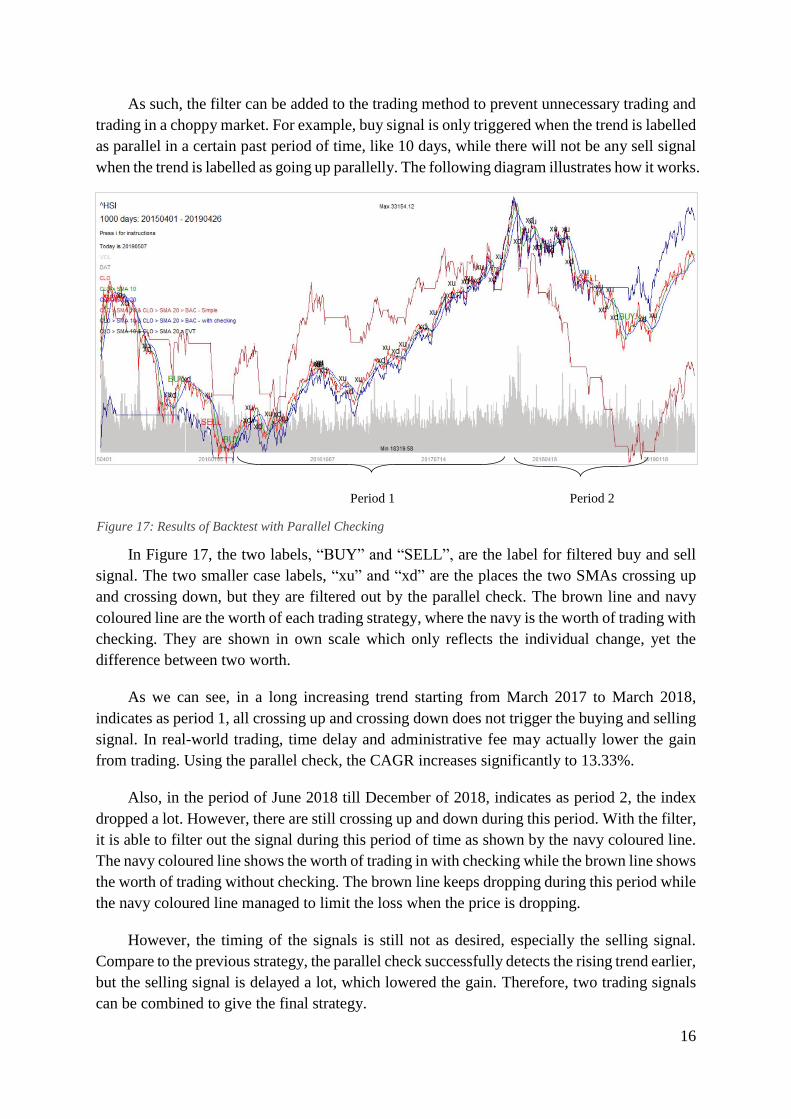
As such, the filter can be added to the trading method to prevent unnecessary trading and
trading in a choppy market. For example, buy signal is only triggered when the trend is labelled
as parallel in a certain past period of time, like 10 days, while there will not be any sell signal
when the trend is labelled as going up parallelly. The following diagram illustrates how it works.
In Figure 17, the two labels, “BUY” and “SELL”, are the label for filtered buy and sell
signal. The two smaller case labels, “xu” and “xd” are the places the two SMAs crossing up
and crossing down, but they are filtered out by the parallel check. The brown line and navy
coloured line are the worth of each trading strategy, where the navy is the worth of trading with
checking. They are shown in own scale which only reflects the individual change, yet the
difference between two worth.
As we can see, in a long increasing trend starting from March 2017 to March 2018,
indicates as period 1, all crossing up and crossing down does not trigger the buying and selling
signal. In real-world trading, time delay and administrative fee may actually lower the gain
from trading. Using the parallel check, the CAGR increases significantly to 13.33%.
Also, in the period of June 2018 till December of 2018, indicates as period 2, the index
dropped a lot. However, there are still crossing up and down during this period. With the filter,
it is able to filter out the signal during this period of time as shown by the navy coloured line.
The navy coloured line shows the worth of trading in with checking while the brown line shows
the worth of trading without checking. The brown line keeps dropping during this period while
the navy coloured line managed to limit the loss when the price is dropping.
However, the timing of the signals is still not as desired, especially the selling signal.
Compare to the previous strategy, the parallel check successfully detects the rising trend earlier,
but the selling signal is delayed a lot, which lowered the gain. Therefore, two trading signals
can be combined to give the final strategy.
Period 1 Period 2
Figure 17: Results of Backtest with Parallel Checking

17
Results
Results of the Final Strategy
First, the buy signal remains the same as the parallel check. It will buy when two short-
term SMAs crosses and the two SMAs are parallel and increasing in the past period of time.
However, for the selling signal, it will sell when it is crossing down, given that the price drops
below the long-term SMA or the two short-term SMA is no longer parallel increase in the past
period of time. The complete logic is shown in Figure 18.
This flowchart clearly shows how the strategy trade for one group of SMAs. It checks
with the indicators included the crossing of SMAs, the parallel checking and the long-term
SMA checking. This flowchart performs the function of the blue predefined function in the
flowchart shown in Figure 1. A sample HTML output of this strategy is attached as Appendix
1, showing a backtest report for SMA 10, 20, 50 and 100, which provides a clear summary of
what parameters and which combination of SMAs is the best.
Figure 18: Flowchart for the Final Strategy

18
Figure 19 below shows the results of the strategy, the labels are the same. The two labels,
“BUY” and “SELL”, are the label for filtered buy and sell signal. The two smaller case labels,
“xu” and “xd” are the places the two SMAs crossing up and crossing down, but they are filtered
out by the parallel check or the long-term check. Lastly, the brown line is worth with simple
crossing while the navy coloured line is the worth of trading with checking.
As shown in Figure 19, it triggered the buy signal immediately at the start of the upward
trend, while the sell signal is at the end of the trend. In the upward trend, indicates as period 1,
it can filter all the sell signal and limit the number of trades, hence, to increases the gain. Also,
in the downward trend, indicates as period 2, it limits the number of selling signal and stop
trading. This limit the loss as shown by the navy coloured line, where it stops decreasing, but
the worth of simple trading (the brown line).
Period 1 Period 2
Figure 19: Results of Backtest using the Final Strategy

19
Overall, trading with checking parallel status significantly increases the worth. Taking
SMA 10, 20 and 50 as an example, the percentage gain increases from 580.9% to 10232.1%.
The CAGR of this strategy increased to 15.4% with the average annual increase in price is only
7.9%. Also, the number of trades is reduced with a significant increase in the percentage gain
of each trade. Details are shown in Table 3.
Table 3: Results of Trading with Final Strategy using SMA 10, 20 and 50
SMA 10, 20 and 50 Total Worth
(%) CAGR (%)
Percentage gain
of each trade (%)
Number of
Trade
Buy and Hold 1052.7 7.85 - -
Trade without checking 580.9 6.11 1.24 209
Trade with checking 10232.1 15.42 14.83 39
The trading filtering out the number of trades increases the percentage gain of each trade,
prevent unnecessary trade and increases the CAGR. The worth gain is almost 10 times the
increase in price over 30 years.
To further illustrate the usefulness
of the filter used, Figure 20 compares the
change of the worth with checking, the
change of the worth without checking
and the change in price. The green line is
the trading with checking and the red line
is the trading without checking. At some
point when the red line is dropping
(2008), the green line can stop trading
and reduce the loss. In the end, the
difference of the worth between the two
strategies is larger and larger as the
backtest is designed to buy as much as it
can when a buy signal is triggered.
Figure 20: The Change in Total Worth for Using the Final Strategy

20
As shown in Figure 21, the CAGR
of trading with checking (thick green
line) is almost always above the CAGR
of trading without checking (red line
behind). The annual change in price is
also indicated as the thin blue line at the
back. In the graph, the CAGR of the
first year (1986) and the CAGR of the
current year (2019) may not be a full
year duration.
When the price significantly
dropped, trading with checking
managed to reduce the lost like in 2008.
However, when the price increases, it
also managed to follow the trend and gain, like 2009. Although there are still ups and downs
for the CAGR of each year, the CAGR over 30 years increased from 6.1% to 15.4%.
Furthermore, not only the average percentage gain is larger after adding a filter, but the
number of days holding the stock also increases when the number of trading reduces. Taking
the combination of SMA 10, 20 and 50 as an example, the average gain of each simple trading
is 1.24% in 209 trade, but the average gain for trading with checking increases to 14.83% with
the number of trades lowered to 39. Figure 22 is a graph plotting the gain of trade against the
number of days holding.
As shown in Figure 22, the number of
days holding it is positively correlated to the
percentage gain, no matter if it is trading with
checking or trading without checking. Also,
mostly trading with checking have a higher
percentage gain and a longer period of
holding the stock. This positive relationship
is probably related to the long-term
increasing trend of the Hang Seng Index, but
have no use on improving the trading
strategies as the days of holding the stock
cannot be known beforehand. This is a result
of the trading strategies but cannot be used to
improve the trading strategies.
Figure 21: CAGR of The Final Strategy
Figure 22: Gain Against the Number of Days Holding using the
Final Strategy

21
Results of Other Groups of SMAs
Table 4 shows the result of a few more combinations. As mentioned in the hypothesis,
this project predicted that a strategy of three SMA, with two short-term and one long-term,
would be a good combination to give sufficient information for predicting the trend. Hence, a
combination of SMA 10, 20 and 50 is better than a combination of SMA 5, 100 and 250. The
full table is attached as Appendix 2.
Table 4: Results of the Final Strategy with Different Combinations of SMA
Simple Trading Trading with checking
Groups of SMA Total
Worth
(%)
CAGR
(%)
Average
percentage gain
of each trade
(number of trades)
Total
Worth
(%)
CAGR
(%)
Average
percentage gain
of each trade
(number of trades)
Buy and Hold 1052.71 7.85 - 1052.71 7.85 -
SMA 5, 10, 50 100.94 2.18 0.55 (411) 5744.19 13.40 6.68 (73)
SMA 5, 100, 250 956.90 7.56 4.00 (72) 389.58 5.03 17.48 (11)
SMA 10, 20, 50 580.92 6.11 1.24 (209) 10232.15 15.42 14.83 (39)
SMA 10, 20, 100 580.92 6.11 1.24 (209) 7185.80 14.18 15.02 (38)
SMA 10, 100, 250 871.04 7.28 4.97 (59) 281.90 4.23 20.5 (10)
SMA 20, 50, 250 743.74 6.82 3.98 (71) 1155.25 8.14 21.61 (20)
The best combinations of the corresponding strategy are bolded, while the numbers below
the simple buy and hold are labelled as red. All the combinations using simple trade are labelled
red, as their worth and annual return is lower than just buy and hold. However, after applying
the strategy, most of the combinations increases significantly in the worth and the CAGR.
This strategy works better with the combination 10, 20 and 50. As the strategy first check
the crossing of two short-term SMA, if the two SMA difference is too large or their days to
average is too long, the crossing is delayed in time when an upward trend occurs. Also, when
the difference between the two SMAs is too large, the shortest SMA will always increase faster
than the longer SMA, hence they are not parallel. They are not increasing at the same rate
steadily, hence will be defined as not parallel according to the algorithm. Lastly, the sell signal
also checks if the two short-term SMAs and the price drops significantly compared to the long-
term SMA, if the long-term SMA is delayed a lot, the effect of change in price is smaller
comparatively. Therefore, combinations like 5, 100 and 250 or 10, 100 and 250 do not perform
as good as others.

22
Results of Trading in Foreign Market
The following attempt to use the above strategy and trade on the foreign stock index. This
check if the strategy can apply to the foreign market. The following apply it to the S&P 500,
CAC 40, and Nikkei 225. Table 5 shows the results of a few groups of SMAs on three indexes.
The best combinations of the corresponding strategy are bolded, while the numbers below the
simple buy and hold are labelled as red.
Table 5: Results of the Final Strategy in Foreign Indexes
S&P500 CAC 40 Nikkei 225
Groups of SMA Results Simple Trading with
checking Simple
Trading with
checking Simple
Trading with
checking
Buy and Hold Total Worth 973.53 190.80 1597.11
Annual Gain 9.45 3.72 5.34
SMA 5, 10, 20
Total Worth
-40.32 715.84 -100 452.46 -100.00 10102.87
SMA 5, 20, 250 64.53 1298.84 -64.93 501.47 1554.38 5794.15
SMA 10, 20, 50 194.52 524.05 -22.43 610.15 1712.18 5652.46
SMA 10, 20, 250 194.52 1141.54 -22.43 911.15 1712.18 5298.13
SMA 10, 50, 250 325.47 1884.40 8.15 643.49 877.60 5641.78
SMA 20, 50, 250 262.92 1801.69 49.17 298.49 499.79 3825.33
SMA 5, 10, 20
CAGR
-1.94 8.31 -100 6.03 -100 8.88
SMA 5, 20, 250 1.91 10.55 -3.52 6.34 5.30 7.78
SMA 10, 20, 50 4.19 7.21 -0.89 6.94 5.47 7.74
SMA 10, 20, 250 4.19 7.21 -0.89 8.24 5.47 7.61
SMA 10, 50, 250 5.66 12.03 0.268 7.11 4.28 7.73
SMA 20, 50, 250 5.10 11.85 1.38 7.67 3.35 6.98
The results of trading in a foreign market are mostly the same as the result of trading with
the Hang Seng Index. However, due to the different market with different nature of the price,
the best combinations of SMA in the different market are different. For example, the best
combinations for the Hang Seng Index is SMA 10, 20 and 50, while the best combinations for

23
the S&P 500 is SMA 10, 50, 250. In addition, the best combinations for a different market are
usually still following the rule two short-term SMA and one long-term SMA.
Also, the strategy has the same behaviour as in the Hang Seng Index. It limits the number
of trades, increases the number of days holding and result for a higher total worth and higher
CAGR. Taking the best combination for the S&P 500, SMA 10, 50 and 250, as an example,
the result from it is quite similar than the result from the Hang Seng Index.
Figure 23 shows the change in worth of the strategy in the S&P 500. The worth with
checking (the green line) increases much faster than the trading without checking (the red line).
It can filter downward trend as shown in 2001 and 2008, as the worth for trading without
checking (the red line) is decreasing, but the checking filters out the signal and limit the loss.
The CAGR of trading without
checking is almost always above the
CAGR of trading without checking. The
CAGR of the first year (1993) and the
current year (2019) may not be a full
year duration. When the price increases,
the trading without checking able to
catch up, like 2004, and gain while
limiting the lost when the price drop
significantly, like 2009.
Interestingly, the annual gain in
each year is almost always positive, with
the CAGR as 12.03% over 25 years.
Figure 23: The Change in Total Worth for Trading in the S&P 500
Figure 24: CAGR for Trading in the S&P 500

24
Figure 25 shows the positive
correlation between the percentage
gain and the number of days holding.
Same as applying the strategy to the
Hang Seng Index, the longer the
number of days holding, the larger the
gain is. Also, the strategy limits the
number of trades from 81 to only 8
trades, with the average percentage
gain increases from 1.92% to 48.74.
Amongst the eight trades, the
smallest gain is 1.88% by holding the
stocks for 52 days, while the largest
gain is 234.63% by holding the stocks
for 1979 days, which is over 5 years.
The strategy is still able to filter out
signals and increase the gain, where then the days of holding the stock also increase.
However, considering the annual increase in the price of the Hang Seng Index and S&P
500 are similar, the total worth and the CAGR of trading in S&P are not as large as trading
with the Hang Seng Index. The strategy is more effective in the local market than other foreign
indexes. This probably due to the parameters in the strategy are tuned with the Hang Seng
Index. For example, the tolerance of the parallel checking, the range allowed for the differences
between two SMAs are set up by doing backtest with the Hang Seng Index, it will work better
when the strategy is applied on Hong Kong Market.
Therefore, the strategy can also be applied to the foreign market, provided that it can still
give the same effect after applying the checking indicators. The most effective combinations
of SMAs in different indexes may be different, due to the different nature of different indexes.
However, the strategy is more effective when trading with the Hang Seng Index, hence proves
that adjustment to parameters is needed when the strategy needed to be applied to different
stocks in a different market.
Figure 25: Percentage Gain Against the Number of Days in the S&P 500

25
Conclusion
This project creates alternative ways as an indicator of trend prediction. It converts some
subjective indicators to objective strategy using programming language, with adjustable
parameters for trading in a different market. By doing multiple backtest with different indexes
in different market, the strategy is proved to be able to gain a larger profit and higher CAGR
compares to trading with crossing only. For example, the concept of parallel is proved to be
reliable and useful in identifying a possible upward trend.
As hypothesize at the beginning, the strategy of using SMAs will be a long-term SMA
with two short-term SMAs, the results prove that this is the most effective ways. The two
additional indicators, parallel checking and long-term checking, are best to work with two
short-term SMAs and one long-term SMA. This project provides a method to generate multiple
indicators between SMAs to gather more information for predicting the trend.
Moreover, this project provides an idea on how to take multiple indicators for the final
decision. The final strategy processes multiple indicators individually, and the final decision is
made by custom logic check with the result of individual indicators as an input. Considering
multiple indicators can help the decision with more information and provide custom adjustment
for certain aim of the strategy. For example, the long-term check in the final strategy is used
for only checking the selling signal, to sell the stock when the price significantly, where a
parallel check cannot identify this problem. This project provides a flexible method of
processing multiple indicators, where more indicators can be added to the logic control without
affecting previous indicators. Other financial processing methods like Bollinger Band or
relative strength index can be included as an individual indicator and include in the final logic
check for the final decision.

26
Evaluation and Further Developments
This project is a success in suggesting alternative ways for trend prediction. The concept
of multiple indicators and parallel as an indicator provides a new way to do trend prediction.
For example, by defining the concept of parallel through a programming language, it allows
this concept to be applied objectively, in which visually parallel SMA is actually a very
subjective feeling. Also, the method of defining the parallel between SMA does not bind to any
market or stock values, as it is calculating the difference between the percentage change of two
SMA. The method can apply to any stocks in any stock market, with only the closing price as
an input.
However, in this project, there are still some rooms for further developments. The trading
strategy is developed and refined under the Hong Kong market. Although it still can make a
profit on foreign market indexes but is not as significant as on the Hang Seng Index. In which
case, the strategy requires different parameters in a different market. For example, the
parameters in defining parallel SMA should be different as the behaviour of price in the
different market may be different. Also, some of the parameters are based on the percentage
changes or percentage differences of price and SMAs, different values of the price may affect
the percentage changes. For example, the “price” of SMA in recent years is more than 30,000
while the “price” of the S&P 500 is lower than 300. The percentage difference between values
will affect some indicators, for example, the long-term check. Therefore, an adaptive threshold
and parameters could be further development for this project.
Second, weighing between individual indicators could be an area for further
developments. For example, when more individual indicators are processed and included in the
strategy, the final logic control might be a probability output instead of a boolean output.
Weighting between different individual indicators can be examined and calculated. The final
decision is not just a buy or sell signal, but a probability on the possible trend of the stock.
However, this requires a lot of hypothesis testing and statistical calculations between different
indicators. When more indicators are included, the calculation of the relation of different
indicators and the price becomes more complicated and harder to estimate. Advanced
modelling and data analysing are needed, which is far more complicated than the aim of this
project but could be further development in the future.

27
Appendix
Appendix 1: Sample HTML Report from Backtesting of the Final Strategy

28

29
Appendix 2: The Results of the Final Strategy Trading in the Hang Seng Index
Table 6: Full Results of the Final Strategy with Different Combinations of SMA
Simple Trading Trading with checking
Groups of SMA Total
Worth (%)
CAGR
(%)
Average percentage
gain of each trade
(number of trades)
Total
Worth (%)
CAGR
(%)
Average percentage
gain of each trade
(number of trades)
Buy and Hold 1052.71 7.85 - 1052.71 7.85 -
SMA 5, 10, 20 100.94 2.18 0.55 (411) 4207.83 12.34 7.29 (63)
SMA 5, 10, 50 100.94 2.18 0.55 (411) 5744.19 13.40 6.68 (73)
SMA 5, 10, 100 100.94 2.18 0.55 (411) 4646.56 12.66 5.61 (83)
SMA 5, 10, 250 100.94 2.18 0.55 (411) 4683.80 12.70 5.62 (83)
SMA 5, 20, 50 681.57 6.56 1.16 (244) 3126.95 11.34 11.76 (36)
SMA 5, 20, 100 681.57 6.56 1.16 (244) 2801.29 10.96 9.13 (45)
SMA 5, 20, 250 681.57 6.56 1.16 (244) 2469.72 10.56 9.80 (41)
SMA 5, 50, 100 1187.82 8.22 2.63 (118) 625.32 6.32 11.97 (21)
SMA 5, 50, 250 1187.82 8.22 2.63 (118) 592.76 6.17 10.53 (23)
SMA 5, 100, 250 956.90 7.56 4.00 (72) 389.58 5.03 17.48 (11)
SMA 10, 20, 50 580.92 6.11 1.24 (209) 10232.15 15.42 14.83 (39)
SMA 10, 20, 100 580.92 6.11 1.24 (209) 7185.80 14.18 15.02 (38)
SMA 10, 20, 250 580.92 6.11 1.24 (209) 7182.83 14.18 14.78 (39)
SMA 10, 50, 100 1143.41 8.11 3.56 (89) 1235.19 8.34 18.15 (21)
SMA 10, 50, 250 1143.41 8.11 3.56 (89) 637.17 6.37 18.73 (18)
SMA 10, 100, 250 871.04 7.28 4.97 (59) 281.90 4.23 20.5 (10)
SMA 20, 50, 100 743.74 6.82 3.98 (71) 1421.70 8.78 16.78 (21)
SMA 20, 50, 250 743.74 6.82 3.98 (71) 1155.25 8.14 21.61 (20)
SMA 20, 100, 250 651.97 6.44 6.13 (43) 613.48 6.26 20.01 (13)
SMA 50, 100, 250 65.79 1.58 3.05 (41) 409.21 5.16 10.9120)
- END -
Related Documents