J. Fluid Mech. (1995), 001. 295, pp. 159-198 Copyright 0 1995 Cambridge University Press I59 An asymptotic two-layer model for supersonic turbulent boundary layers By J. HE, J. Y. KAZAKIA AND J. D. A. WALKER Department of Mechanical Engineering and Mechanics, Lehigh University, Bethlehem, PA 18015, USA (Received 20 March 1992 and in revised form 16 February 1995) An asymptotic analysis of the compressible turbulent boundary-layer equations is carried out for large Reynolds numbers and mainstream Mach numbers of O(1). A self-consistent two-layer asymptotic structure is described wherein the time-mean velocity and total enthalpy are logarithmic within the overlap zone but in terms of the Howarth-Dorodnitsyn variable ; the proposed structure leads to a compressible law of the wall for high-speed turbulent flows with surface heat transfer. Simple outer-region algebraic turbulence models are formulated to reflect the effects of compressibility. To test the proposed asymptotic structure and turbulence models, a set of self-similar outer-region profiles for velocity and total enthalpy is obtained for constant-pressure flow and for constant wall temperature; these are combined with wall-layer profiles to form a set of composite profiles valid across the entire boundary layer. A direct comparison with experimental data shows good agreement over a wide range of conditions for flows with and without surface heat transfer. 1. Introduction Prediction of high-speed compressible turbulent flows near solid boundaries is hampered by several practical difficulties, some of which are associated with the uncertain quality of available turbulence models, while others are primarily computational in nature. Algebraic models represent the simplest type of mathematical models that describe the effect of turbulence near a solid wall, but even when higher- order closure schemes are contemplated, many of the critical modelling issues concern the functional form of the velocity and temperature profiles in the overlap zone near the surface, where both profiles exhibit a logarithmic dependence on normal distance from the wall. Examples of modern algebraic models include the Cebeci-Smith (1974), the Baldwin-Lomax (1978), and Johnson-King (1985) models. The essence of these formulations is a simple ramp function for eddy viscosity in the outer part of the boundary layer (see also Mellor & Gibson 1966)which behaves linearly in distance from the wall near the surface and then abruptly changes to a constant whose value depends on the local flow conditions. Sometimes ‘intermittency ’ factors are also introduced in order to reduce the eddy viscosity to zero far from the wall, but such modifications are generally found to have relatively little impact on the shape of the velocity profile. Eddy viscosity models are typically modified to a mixing length formulation in the wall layer (between the surface and the overlap zone); the mixing length is defined to be linear in the overlap zone, but is then reduced toward the wall through multiplication by the Van Driest damping factor (see, for example, Cebeci & Smith 1974). It is well known that algebraic turbulence models yield good predictions for attached turbulent flows (see, for example, Kline, Cantwell & Lilley 1981) at low to moderate

Welcome message from author
This document is posted to help you gain knowledge. Please leave a comment to let me know what you think about it! Share it to your friends and learn new things together.
Transcript
J . Fluid Mech. (1995), 001. 295, pp. 159-198 Copyright 0 1995 Cambridge University Press
I59
An asymptotic two-layer model for supersonic turbulent boundary layers
By J. HE, J. Y . KAZAKIA AND J. D. A. WALKER Department of Mechanical Engineering and Mechanics, Lehigh University, Bethlehem,
PA 18015, USA
(Received 20 March 1992 and in revised form 16 February 1995)
An asymptotic analysis of the compressible turbulent boundary-layer equations is carried out for large Reynolds numbers and mainstream Mach numbers of O(1). A self-consistent two-layer asymptotic structure is described wherein the time-mean velocity and total enthalpy are logarithmic within the overlap zone but in terms of the Howarth-Dorodnitsyn variable ; the proposed structure leads to a compressible law of the wall for high-speed turbulent flows with surface heat transfer. Simple outer-region algebraic turbulence models are formulated to reflect the effects of compressibility. To test the proposed asymptotic structure and turbulence models, a set of self-similar outer-region profiles for velocity and total enthalpy is obtained for constant-pressure flow and for constant wall temperature; these are combined with wall-layer profiles to form a set of composite profiles valid across the entire boundary layer. A direct comparison with experimental data shows good agreement over a wide range of conditions for flows with and without surface heat transfer.
1. Introduction Prediction of high-speed compressible turbulent flows near solid boundaries is
hampered by several practical difficulties, some of which are associated with the uncertain quality of available turbulence models, while others are primarily computational in nature. Algebraic models represent the simplest type of mathematical models that describe the effect of turbulence near a solid wall, but even when higher- order closure schemes are contemplated, many of the critical modelling issues concern the functional form of the velocity and temperature profiles in the overlap zone near the surface, where both profiles exhibit a logarithmic dependence on normal distance from the wall. Examples of modern algebraic models include the Cebeci-Smith (1974), the Baldwin-Lomax (1978), and Johnson-King (1985) models. The essence of these formulations is a simple ramp function for eddy viscosity in the outer part of the boundary layer (see also Mellor & Gibson 1966) which behaves linearly in distance from the wall near the surface and then abruptly changes to a constant whose value depends on the local flow conditions. Sometimes ‘intermittency ’ factors are also introduced in order to reduce the eddy viscosity to zero far from the wall, but such modifications are generally found to have relatively little impact on the shape of the velocity profile. Eddy viscosity models are typically modified to a mixing length formulation in the wall layer (between the surface and the overlap zone); the mixing length is defined to be linear in the overlap zone, but is then reduced toward the wall through multiplication by the Van Driest damping factor (see, for example, Cebeci & Smith 1974).
It is well known that algebraic turbulence models yield good predictions for attached turbulent flows (see, for example, Kline, Cantwell & Lilley 1981) at low to moderate
160 J . He, J . Y. Kazakia and J. D. A . Walker
subsonic speeds, where an extensive base of reliable experimental data is available to validate the computed results. Such models are often used almost without modification in prediction methods for supersonic turbulent boundary layers (see, for example, Talcott & Kumar 1985), the implicit assumption being that a compressible ‘law of the wall’ exists which is similar to the incompressible form (see, for example, Viegas, Rubesin & Horstman 1985; Carvin, Debieve & Smits 1988). However, the generalization of the ‘law of the wall’ to compressible flow has been somewhat controversial, and a number of different functional forms have been proposed (see, for example, Van Driest 1951 ; Rotta 1960; White & Christoph 1972; White 1992). Perhaps the most popular formulation is the ‘effective velocity’ approach of Van Driest (1951); this constitutes a particular extension of the incompressible formulation, wherein the mixing length for compressible turbulence is also assumed to be linear in physical distance from the wall within an anticipated overlap zone between the wall layer and outer region. Upon accounting for a variation in density, an incompressible form of the law of the wall is ultimately derived but in terms of an effective velocity, obtained from the actual mean streamwise velocity through a transformation involving an inverse sine function. This has come to be known as the Van Driest transformation and strictly should be expected to yield only a localized description of the velocity profile (since it is based on a specific type of mixing-length model within the overlap zone). However, Make & McDonald (1968) found that a substantial amount of adiabatic- wall profile data could be collapsed when an effective velocity was defined across the entire boundary layer. Although the approach appears to be less impressive when there is heat transfer at the wall (Maise & McDonald 1968), the Van Driest transformation is used extensively in analysis of profile data and, sometimes, to infer values of skin friction at the surface from measured velocity profile data. A critical discussion of the transformation is given by Fernholz & Finley (1980).
There are some aspects of the Van Driest transformation which could be regarded as disadvantageous. First the transformation is based on a specific type of turbulence model (mixing length) in the overlap zone and other types of models, such as eddy viscosity, produce a different functional form for compressible flow for the velocity in the overlap zone (Degani et al. 1991); this situation may be contrasted with the case of incompressible flow where all turbulence models are implicitly constructed to produce a universal logarithmic law of the wall. A second point is that it is difficult to assess the circumstances under which the Van Driest transformation becomes invalid with increasing surface heat flux and/or increasing mainstream Mach number. Lastly the inverse sine behaviour contained in the velocity distribution for this model can be somewhat awkward in a numerical prediction algorithm. For these reasons, a principal objective of the present study was to search for an alternative, and potentially simpler, theoretical description of the compressible turbulent boundary layer.
It is well known (Stewartson 1964) that the Howarth-Dorodnitsyn variable Y defined by
Y = r’dn, 0 Po
is an appropriate normal coordinate in the description of compressible laminar boundary layers; here p is the density, po is a reference density, and n measures physical distance from the wall. The variable Y may be interpreted as a density-averaged distance from the wall and the motivation behind such compressibility transformations is to convert the problem into a simpler form similar to incompressible flow. It might be expected that a similar transformation can be used in compressible turbulent flows
Asymptotic two-layer model for boundary layers 161
and this question has been taken up by Burggraf (1962), Crocco (1963) and Coles (1964), among others, who have discussed a variety of possible approaches. Implicit in many of these studies is the idea of a ‘reference condition’ at which the variable thermodynamic properties are to be evaluated, in the hope that the gross properties of the boundary layer may be represented by corresponding established incompressible formulae. For laminar compressible boundary layers, the ‘reference’ density po in equation (1) is usually taken to be the density at the wall, but a dilemma exists for turbulent flows since a suitable reference density is not immediately apparent. In the outer portion of the turbulent boundary layer, the mean density can be expressed as a perturbation from the mainstream value. On the other hand, even for an adiabatic wall, the density at the surface is often substantially different from the mainstream value and there is an intense variation in p across the inner wall layer. Consequently, a difficulty exists in defining a density which is characteristic of both portions of the boundary layer, and this issue will be subsequently addressed here.
A main thrust of the present study is to introduce the Howarth-Dorodnitsyn variable, with a suitable choice for po, in the description of the turbulent boundary layer and further to propose that the mean velocity profile in the overlap zone may be conveniently represented in a form which is logarithmic in Y. Starting from this premise, it is shown that a self-consistent asymptotic two-layer structure, valid in the limit of large Reynolds number, Re, may be constructed. To obtain velocity and temperature profiles, a simple algebraic turbulence model, which is a generalization of existing incompressible turbulence models, is formulated. The eventual test of the proposed structure which is carried out here constitutes a direct comparison with experimental skin-friction velocity and total-temperature profile data. These com- parisons strongly support the premise of a universal compressible law of the wall in terms of the Howarth-Dorodnitsyn variable.
Established theoretical results for the temperature distribution in compressible boundary layers are relatively scarce. For low-speed subsonic flows, the data for the static temperature distribution (Weigand 1978) clearly display a logarithmic behaviour in the overlap zone. However, the value of the slope of the temperature profile in the overlap zone (unlike that of the velocity profile), appears to vary with pressure gradient and local flow conditions (Weigand 1978). In supersonic boundary layers, the total enthalpy plays a similar role to the static temperature at low speeds, but direct measurements of this quantity, particularly in the overlap zone, are relatively rare. Consequently, it is somewhat difficult to estimate accurately the slope of the total enthalpy profile in the overlap zone from existing experimental data, or in some cases to ascertain even if the total enthalpy is logarithmic there. At subsonic speeds, the turbulent heat flux terms in the energy equation are usually modelled by an algebraic model in which an ‘eddy conductivity’ is related to the eddy viscosity through a turbulent Prandtl number. However, inferred distributions of the turbulent Prandtl number are not generally found to be constant, even in low-speed thermal boundary- layer flows (Crawford & Kays 1980, p. 226), and often additional semi-empirical relations are introduced in prediction methods so that the turbulent Prandtl number varies across the boundary layer. For high-speed compressible flow, similar modelling concepts are often employed, as well as various semi-theoretical versions of the Crocco relations (Fernholz & Finley 1977). In the present study, one goal was to treat the thermal problem independently from the velocity problem and without introducing a turbulence model based explicitly on either a turbulent Prandtl number, or semi- theoretical version of the Crocco integral. Here a self-consistent structure is presented for the total enthalpy distribution in the boundary layer, which is logarithmic in the
162 J . He, J . Y. Kazakia and J. D. A . Walker
overlap zone in the variable Y ; a formula for the slope of the total enthalpy is derived, as well as a relationship from which the surface heat transfer at the wall can be evaluated. Again, the proposed structure is tested by comparing total enthalpy directly with the recent experimental data of Carvin (1988), as well as other existing data sets catalogued by Fernholz & Finley (1977, 1981).
One motivation of this investigation was to provide a theoretical foundation for more efficient algorithms for the prediction of high-speed compressible turbulent boundary layers. For subsonic two-dimensional boundary layers, it is well-known that the inner wall layer exhibits a self-similar behaviour (Fendell 1972). In the embedded- function methodology described by Walker, Werle & Ece (1991), the self-similar wall- layer structure is incorporated in a prediction method by representing the mean velocity and total enthalpy distributions by analytical profiles across the entire wall layer; the profile models are derived through consideration of the coherent structure and dynamics of the near-wall flow (Walker et al. 1989; Smith et al. 1991). In the embedded-function algorithm, a conventional numerical solution is matched sys- tematically to the wall-layer functions and Walker et al. (1989) demonstrate that up to a 50 % reduction in total mesh points (as well as computational effort) can be achieved with no degradation in accuracy, as compared to a conventional scheme that computes the flow all the wall to the wall. For three-dimensional subsonic turbulent boundary layers, a similar but more complicated similarity structure exists in the wall layer for attached turbulent flows (Degani, Smith & Walker 1993; Degani & Walker 1993).
Because the embedded-function approach requires the smooth joining of an exterior numerical solution to a set of inner-region functionals, which are logarithmic near the surface, the numerical algorithms involved are not straightforward. A crucial step in the methodology is the determination of the appropriate asymptotic scaling laws for the velocity and total enthalpy in the overlap zone. This is carried out in the present paper through the development of asymptotic expansions, which describe the structure of the solution of the compressible boundary-layer equations for large Reynolds number. The turbulence models used in the present study for the outer-region are simple eddy viscosity and conductivity models and are similar to the Cebeci-Smith (1974) and Baldwin-Lomax (1978) incompressible models; their functional form for high-speed compressible flow is guided by the results of the present asymptotic analysis. These models have been selected here as the simplest possible outer algebraic models in order to demonstrate the concepts involved. For the wall layer, a set of embedded functions for velocity and total enthalpy is described, as well as matching conditions in the overlap zone from which skin-friction and heat-transfer coefficients can be found. In order to test the results of the asymptotic theory, as well as the turbulence models, a limiting case is considered corresponding to self-similar profiles that evolve in a constant-pressure flow with heat transfer; in this situation, the governing equations in the outer region of the boundary layer reduce to ordinary differential equations, for which either exact analytical solutions or accurate numerical solutions may be found. The outer-layer profiles are then matched to the embedded wall-layer functionals to form a set of composite profiles of velocity and total enthalpy across the entire boundary layer. These profiles were then compared directly with experimental data over a range of Mach numbers and the agreement is very encouraging.
The turbulent transport of thermal energy is commonly modelled utilizing the concept of a turbulent Prandtl number Pr,. Measurements suggest that (at least in low- speed flows) Pr, is close to constant in the outer layer but exhibits a significant variation across the wall layer (see, for example, Crawford & Kays 1980, p. 226). This type of
Asymptotic two-layer model f o r boundary layers 163
model is also considered here, and it is shown that if a constant turbulent Prandtl number model is used in the outer layer, the value cannot be specified arbitrarily. For constant-pressure flow, an expression is derived for the outer-layer value of Pr, as a function of Mach number and Prandtl number. The predicted value of Pr, for low- speed airflow is in good agreement with previous empirical estimates.
The plan of the paper is as follows. In $2, the governing equations for the compressible turbulent boundary layer are described in terms of the Howarth- Dorodnitsyn variable. A general analysis of the leading-order wall layer is given in $ 3 while the outer layer is discussed in $4. The compressible turbulence models for the outer layer are described in $ 5 . In $6, the special set of profiles for velocity and total enthalpy in a constant-pressure flow are given. The reference condition and the constant turbulent Prandtl number model are described in $97 and 8 respectively. Detailed comparisons with experimental data are discussed in $ 9.
2. Governing equations In this section, the basic equations governing either a two-dimensional or an
axisymmetric nominally steady turbulent boundary-layer flow are summarized. Dimensionless variables are defined utilizing a reference length LFef, a speed UFef, a viscosity pFef, a density pFef.and static temperature TFef; in addition the total enthalpy His made dimensionless with respect to c3 TFef, where c; (the specific heat at constant pressure) is assumed constant. The Reynolds number, reference Mach number and Prandtl number are defined by
Here R is the gas constant and y = cf/c,* is the ratio of specific heats, which is assumed constant; p* and k* are the dimensional absolute viscosity and thermal conductivity. The Prandtl number is assumed constant and 0(1), with the Reynolds number being large. The ideal gas law (in dimensionless variables)
P = pT/yM,2ep (3)
is taken as the equation of state. An orthogonal coordinate system is defined with (s, n ) measuring distance along the
contour of the wall and normal to it, respectively, with (u, v) being the corresponding mean velocity components. The governing equations may be written in a simplified form using the Howarth-Dorodnitsyn transformation (Stewartson 1964) defined by eauation (1 ) and
Let r(s) denote the dimensionless radius of revolution for an axisymmetric body (with respect to some typical radius r,*) and, for the two-dimensional case, take r = 1 in what follows. It is easily shown that the compressible turbulent boundary-layer equations may be written
a a as ay -(ru)+-(rC) = 0, ( 5 )
164 J. He, J . Y. Kazakia and J. D. A . Walker
where here (and throughout) a subscript e denotes a known quantity at the boundary- layer edge; in addition, 7 and q are the total stress and energy flux (toward the surface) defined by
respectively, with CT and q5 denoting the Reynolds stress and a turbulent energy flux defined by ~ ~
in terms of time averages of fluctuating quantities. The boundary conditions are g = - ~ u ' v ' , $ = -pv'H', (9)
u=v"=O at Y=O; u+Ue as Y+m, (10a, b) H = H w at Y = O ; H+He as Y+m, (1 1 a, b)
for known wall temperature; for an adiabatic wall, (1 1 a) is replaced by aH/a Y = 0 at Y=O.
For steady flow, He is a constant and the Mach number in the mainstream is related
The total enthalpy H may be written in terms of the static temperature T and u (in the variables) according to present dimensionless
and it is easily shown
- = [l ++(y- 1)M3 --fa- . T, T ([ :J
Since the pressure does not vary to leading order across the boundary layer, it follows from ( 3 ) that p,/p = T/T,. Consequently, the density ratio of the right-hand side of (6) may be general be replaced by the right-hand side of (14), and the pressure gradient term in (6) can be shown to be as follows:
Lastly, the viscosity p is taken to be a known function of temperature alone, such as the Sutherland relation, or the empirical formula due to Keyes (1952) discussed by Fernholz & Finley (1977). From (1 5), it may be inferred that the compressible problem in (5E(7) is defined solely in terms of the unknowns u, 6 and H. Simpler subsets of these equations in the limit Re+ co will now be identified.
3. The wall layer
usual manner according to Consider first the wall layer and define the dimensionless friction velocity u, in the
Asymptotic two-layer model for boundary layers 165
For incompressible turbulent flow, Fendell (1 972) and Mellor (1972) have presented particularly insightful analyses which identified the appropriate length and velocity scales in the wall layer for large Reynolds numbers; their work reproduces the familiar classical results and a similar approach will be used here. For the compressible wall layer, it is assumed that, with the compressibility transformation ( 1 ) and characteristic fluid properties po and ,uo, the velocity in the wall layer is a function of 7,, po, ,uo and Y, as for incompressible flow; this suggests a functional relation of the form
u = Urof@OU7, Y/PJ, (17) where uTo is a general velocity scale defined by
Note that u,, reduces to u, in the limiting case of incompressible flow or if the characteristic density po is taken equal to p, for compressible flow.
A central assumption in the present study is that the velocity in the wall layer (as for incompressible flow) may be formally defined in terms of a scaled inner variable by
u,,, = ( ~ , / ~ o ) l ’ ~ = PO)^" u7. ( 1 8 )
u=u,,U+(Y+)+ ..., Y + = Y/Ai, (19a7 b )
where di(Re) is proportional to the thickness of the wall layer and the profile function U + satisfies
1 a Y+ K
- 1 at Y+ = O ; U+ --logY++Ci as Y++co. (2Oa-c) au+ u+=o, --
The second of these conditions is a conventional convenient normalization. In the logarithmic law ( ~ O C ) , K is the von KarmBn constant and Ci is the inner-region log-law constant, which are usually assumed to have universal values of K = 0.41 and Ci = 5.0. Using (l), (16), (18) (19a) and (20b), it is readily shown that Ai is defined by
Ai = to ~w/@iReu7o). (21) It is easily verified that for incompressible flow A, reduces to ,u,/@, Reu,) and (19b) becomes the definition of the conventional inner variable y+ = pz u,* n* /pz ; here the asterisk superscripts denote the corresponding dimensional quantity. For compressible flow, Y+ is proportional to y+ close to the wall; elsewhere in the wall layer, the scaled normal variable Y+ implicitly contains a density variation through the definition of Y in ( 1 ) .
For low-speed flows (see, for example, Fendell 1972 and Smith et al. 1991), it is well known that, because the wall layer is thin and the streamwise velocity is small, the viscous and Reynolds stress terms are dominant in (6) in the limit as Re+ GO, while both the convective terms and streamwise pressure gradient are negligible to leading order. These same features of the compressible wall layer may easily be checked using the scalings that will be adopted here; a more formal development is given by He (1993). Equation (6) then reduces to a7/aY+ = 0, and thus the total stress is constant across the wall layer to leading order and equal to the value at the wall; therefore in the wall layer 7 = p, u,2 = po u:, and using @a), it follows that
According to ( ~ O C ) , the velocity is taken to be logarithmic in Y+ in the overlap zone (where Y++ co) and it follows that
‘ ~ + p ~ u ~ , = p ~ u ~ as Y++co, (23)
166 J . He, J . Y. Kazakia and J . D . A . Walker
to leading-order. It is important to note that any Reynolds stress model for the outer layer must behave according to (23) in the overlap zone.
In view of (23), the Reynolds stress in the wall layer is expanded as
0- = p o U ~ o a l ( Y + ) + . . . , (24) where cr1 must satisfy
a , = O at Y+=O; g I + l as Y++oo. (25 a, b)
which relates the two profile functions U + and g1 (one of which must be specified to define a specific closure model in the wall layer). As shown in Appendix A for gases in which the viscosity is a function of temperature alone, the Chapman-Rubesin density viscosity law pp = pwpw (Stewartson 1964) may be utilized in the wall layer; this results in a further simplification of (26). Since the convective terms do not enter the leading- order wall-layer equations, the dependence of the solution on the streamwise variable s can at most be parametric and v1 and U+ are principally functions of Y+. In this study the turbulence model that will be used for the wall layer consists of direct specification of a profile function for U+ to be described in $5.
Now consider the thermal problem. Again, the convective terms are negligible to leading order in the wall layer and (7) reduces to aq/aY+ = 0. Consequently q is constant to leading order across the wall layer and equal to the value at the wall qw. It follows from (8 b) that
But since u and $ vanish at Y+ = 0
Thus qw denotes a dimensionless heat flux at the wall (from fluid to the wall; see Appendix B) defined by
where asterisk superscripts denote dimensional quantities and kz is the dimensional thermal conductivity of the fluid at the wall.
It will subsequently be shown (in $4) that qw is U(U:~/ U:) and since u is U(uT ) in the wall layer, it is easily verified that the third term on the right-hand side of (27) is negligible to leading order, provided (uTo/ U,) < 1. Thus the following expansions for total enthalpy and the turbulence heat flux term are indicated:
H = H,+%o++ ..., $ = qw$l+... Po UT0
Here $1 and O+ are profile functions of Y+ and Pr, one of which must be specified to define closure for the total enthalpy equation in the wall layer. The analysis of Weigand (1978) and Walker, Scharnhorst & Weigand (1986) indicates that the profile function B+ should exhibit a dependence on the square root of Prandtl number according to
B+ = O+( Y i ) , Y i = Pr”’ Y+. (3 1)
Asymptotic two-layer model for boundary layers I67
In terms of YB+, (27) gives 1 pp ao+
Prllz pw pw a Y; + # l = 1, __--
which also may be simplified using the Chapman-Rubesin law (Appendix A). Here 8+ and #1 must satisfy
(344 b) 1
O+--logY,f+B,, #1+1 as Y,f+co.
For total enthalpy, K~ plays the role of the von Karman constant in the velocity distribution. However, it will be shown (in $4) that K~ is not constant in general and depends on local flow conditions.
It is worthwhile to emphasize that the general relationships described in (32)-(34) are independent of a specific thermal closure model; furthermore, any model adopted for the turbulent energy flux # in the outer layer must conform to the behaviour
in the overlap zone between the outer region and the wall layer. In this study, the turbulence model used for the wall layer is a profile function O+ that will be described in $ 5 , where formulae for K~ and Bi will also be developed.
Kg
#+qw as Y,++co, (35)
4. The outer layer In the outer layer, the normalized variable 7 = Y / d o is introduced; here do@, Re) is
a scaling parameter proportional to the local boundary-layer thickness which will be selected subsequently. A stream function is defined by
which satisfies (9, and the streamwise velocity and total enthalpy are written in a defect-law form according to
, H = He(l +q* GI+...). (37a, b)
Here 4 and 8, are defect functions of (s, 7) to be determined and the gauge functions u* and q* are defined by
so that the defect terms have the same order as in the wall layer in order to permit matching to the profiles in (19a) and (30a); it will subsequently be shown that both u* and q* are small for Re large. The corresponding expansion for the stream function is
In addition, the total stress and energy flux in the outer layer must be comparable to the corresponding quantities in the wall layer, and upon comparison with (24) and (30b), 7 and q are expanded according to
where T,, Ql+ 1 as 7 + 0 in order to match the wall-layer solution.
(39) II. = do(s, Re) ue(s) 4s ) [7 + U* E;(s, 7) + * * *I .
7 = p 0 u ~ , ~ ( s , q ) + . . . , q = q,Q,<s,q>+..., (40 a, b)
168 J . He, J . Y. Kazakia and J , D. A . Walker
The defect functions in (37) must satisfy
in order to match to the mainstream, and near the wall both are taken to be logarithmic according to
ar;, 1 1
a7 K KO ---log7+C,, O,--logv+B, as 7+0,
in accordance with the present proposed structure; this logarithmic behaviour ensures the existence of an overlap region between the inner and outer layers. Note that the general form of these conditions applies for any attached turbulent boundary-layer flow; C, and B, are functions of s (to be found) and the actual streamwise distribution of these quantities is strongly influenced by the particular outer-region turbulence model adopted.
Matching of the velocity profile in the overlap zone is carried out using the asymptotic forms (20c) and (42a), and it is easily shown, using (19a) and (37a) that
- 1 = !log L L Re U, u* A ,
u* K w P w (43)
This velocity matching condition relates the skin friction to the outer scale A, , as well as the profile parameters C, and Ci. Similarly matching of the inner and outer total enthalpy profiles using (30a), (34a), (37b) and (42b) yields the thermal matching condition
1-I, - log LL Re U, u* A , + B, - B,, 4* K O ( 4 w P w
(44)
where I, = Hw/He. This condition relates the heat flux at the surface to the parameters associated with the velocity and total enthalpy profile.
It is easily verified upon substitution of (37a), (39) and (40a) into the momentum equation (6) that, in order to have a balance the total stress and convective terms, A , = O(u,). It follows from (43) and (44) that
u,+O, q*+O as Re-tco. (45)
Furthermore it is evident from (43) and (44) that for K~ = O( 1) and I, =l 1, q* = O(u,). Substituting the expansions (37) and (40) into (6) and (7) and neglecting quadratic terms in the small quantities u* and q* leads to
where the prime denotes differentiation with respect to s. It may be noted that for specified wall temperature the thermal match condition (44)
contains two additional unknowns, K~ and q*. In a conventional approach (see, for example, Cebeci & Smith 1974), some type of turbulent Prandtl number formulation is used to define a turbulent heat flux model for the outer region which thereby implicitly defines a constant value for K ~ . This is one of two types of models which will
Asymptotic two-layer model for boundary layers 169
be considered subsequently, but for the present the analysis will remain general. In the limit of large Reynolds number, the logarithmic terms dominate the right-hand side of (43) and (44), and it follows that
Consequently K~ can be expected to exhibit a significant dependence on local conditions (Weigand 1978).
In the present study, the value of K* is taken to be defined by the asymptotic result (48); this effectively fixes the most significant aspect of the turbulence model for the total enthalpy equation, namely the slope of total enthalpy in the overlap zone. The thermal match condition (44) serves to determine the heat-transfer parameter q* for given values of Prandtl number, wall temperature, and u,; the characteristics of the outer- and inner-layer profiles enter through the log-law parameters B, and Bi respectively. In practice, K* may be calculated from (48) (with K = 0.41) for a given estimate of q* and u*, and then q* is updated using the full thermal match condition (44); both quantities may then be refined through an obvious iteration (Weigand 1978). An alternative approach was used here. In order to ensure matching of the total enthalpy profile, the full thermal condition (44) must be satisfied. Using (43) to eliminate A , from (44) and with (48), it is easily shown that
In the turbulence models that will be described in $ 5 , both B, and Bi are implicit functions of K~ and, consequently, (49) becomes a nonlinear equation for K ~ .
It is possible to express K* in terms of a Stanton number defined by
and (48) gives K~ = ~p~ St/(po u",. However, a disadvantage of the Stanton number in a high-speed compressible flow is that St may become very large for a heated wall when H , is close to He. A heat transfer parameter Q, suggested by Fernholz & Finley (1977) avoids the difficulty and is defined by
9, Po Q, = = -4* u*, ~w ue He ~w
which is bounded in all situations; K* can be expressed in terms of Q, by
5. Turbulence models The asymptotic structure described in $03 and 4 is independent of any particular
turbulence model. However, in order to produce profiles that can then be compared with experimental data, it is necessary to introduce specific turbulence models; here relatively simple algebraic models will be formulated for the outer layer. Models, such as the Cebeci-Smith (1974) and the Baldwin-Lomax (1978) eddy-viscosity formulations, were originally developed and refined for relatively low-speed flows.
170 J. He, J . Y. Kazakia and J . D . A . Walker
Such models are often utilized in high-speed compressible flow. Here some basic modifications will be considered to account for the significant density variations that can occur in supersonic boundary layers and at the same time cast the models in terms of the Howarth-Dorodnitsyn variable. Simple algebraic models are of the form
where e and eH are the total effective viscosity and conductivity, respectively. Note that q is sometimes written in terms of the gradient of the static temperature and that for low Me both formulations are equivalent. Throughout the bulk of the outer layer, 7 and q consist primarily of Reynolds stress and turbulent flux respectively. Consider first the eddy-viscosity function. In terms of the Howarth-Dorodnitsyn variable Y defined in (1) and the scaled outer variable
7 = peau/an, q = pc, aH/an, (53a, b)
From (37a) and (42a), it follows that
But in the wall layer the total stress is constant with 7 = pw u," = po u:~, and in order to provide a smooth transition between the inner and outer layers, the eddy viscosity function must have the following form for small 7:
This linear behaviour in Y is a necessary feature of all proper outer-region models and is required to produce the assumed logarithmic behaviour in the mean profile in the overlap zone. However, an additional important aspect of (56) is the functional dependence on the density that is mandated near the overlap zone.
For larger values of Y, the linear dependence on Y must be modified and simple far- field eddy viscosity formulae for low-speed compressible flow are normally of the form
Here K is a constant that is usually assigned a value of K = 0.0168 and x is a function e,, = Kx. (57)
of s such that
for the Cebeci-Smith (1974) and the Baldwin-Lomax (1978) models, respectively. Here 6* is the kinetic (or incompressible) displacement thickness defined by
For the Baldwin-Lomax (1978) model, nmaX is the physical distance for the wall where the function F = n lau/anl achieves a maximum, with FmaX being the corresponding value of F; C,, is a constant (having a value of about 1.6) which has been adjusted (see Baldwin & Lomax 1978) so that the model produced has essentially similar results to the Cebeci-Smith (1974) model at low Mach numbers; recently He & Walker (1995) have shown that a value of C,, = 1.73 produces an exact correspondence between the two models for constant-pressure flows. The linear variation of the eddy viscosity for small 7 is normally joined to (57) as a simple ramp function, with the juncture being determined as the location where the two formulae give the same value. It is noted in
Asymptotic two-layer model for boundary layers 171
passing that mixing-length formulations are commonly used close to the wall (see, for example, Cebeci & Smith 1974); however, for low-speed flows, u is logarithmic in the overlap zone and the mixing-length formulation is equivalent to using an eddy- viscosity model which is linear in y in the near-wall region.
For high-speed compressible flow, a corresponding simple formulation is desired. In the present study, three requirements of the model were considered important : (i) the asymptotic behaviour in (56) for small 7; (ii) a far-field behaviour that reduces to (57) for low Mach numbers; and (iii) wide applicability over a range of Mach numbers without introducing additional empiricism. There are a number of functional forms that would fulfil these three requirements, and many of these were tested pragmatically in this study. In the adopted compressible models, it proved convenient to carry the variation in density indicated by (56) across the outer layer and the eddy-viscosity function was written in the form
e = - u, S*2(7). P2
In this manner the correct form of the density variation near the overlap zone mandated by (56) is contained in the model; thus near the overlap zone, e varies rapidly but then is almost constant in the rest of the outer layer. In (60), 2 is the simple ramp function defined by
where q m denotes the intersection of the two functions in (61) with
Here the values of the parameter K are given by
for the extended Cebeci-Smith (1974) and Baldwin-Lomax (1978) models, respectively; in (63), n,,, was taken to be in terms of the physical distance n from the wall as in the corresponding incompressible model. It may be noted that the S* in (60) is still defined by (59) and may be viewed as a kinetic displacement thickness whose value is principally associated with the velocity distribution. The actual displacement thickness for compressible boundary layers contains the influence of both density and velocity and was judged to be unsuitable for scaling turbulent velocity profiles over a range of surface heat transfer conditions. A variety of other models were also rejected on the basis of subsequent data comparisons; these included utilizing different factors of density in (60) and/or a length scale similar to (59) but with the integration variable being Y.
Following similar arguments to those used for the eddy-viscosity function, it is easily shown using (35) and (53 b) that the compressible eddy conductivity function eH must have the following form for small 7:
K = 0.0168 or K = 0.0168[C,,nm,,~~,,/(UeS*)] (634 b)
For larger values of 7, the linear dependence on q must be modified and a simple far- field eddy-conductivity formula that has been utilized for low-speed subsonic compressible flow is (see Weigand 1978 and Walker et al. 1986)
eHo = Kh Ue S*. (65)
172 J . He, J . Y . Kazakia and J . D. A . Walker
Again, a generalization to high-speed compressible flow is sought which conforms to the condition (64) and reduces to (65) in the outer part of the boundary layer for low Mach numbers. The eddy-conductivity formula adopted is consistent with the form of (60) and is
where 2, is the simple ramp function
Here yl is defined by (62a) and i j , = K , ~ J K ~ . Two types of model may be considered for the total enthalpy equation in the outer
layer. In the first of these, Kh is taken to be specified constant and the value of K~ is determined from (48). Extensive comparisons with temperature profile data in subsonic boundary layers carried out by Weigand (1978) for flows with and without pressure gradients suggest a universal value of Kh = 0.0245 ; this value was used in much of the subsequent data comparisons in this study. A second type of model is more conventional and is based on a constant turbulent Prandtl number Pr,, which is defined by Pr, = c/eH. If the turbulent Prandtl number is assumed to be constant across the outer layer, it follows that
A value of Pr, E 0.9 is often assumed for low-speed flows. It will be shown in $8 that Pr, cannot be specified arbitrarily; such a model is only self-consistent provided that Pr, satisfies a relation in which it is defined as a function of Me and Pr.
Upon substituting (53), (60), and (66) into (46) and (47), it follows that the outer- layer defect profiles satisfy
K / K h = K / K o = Pr,. (68)
where the coefficients in these equations are given by
Note that it follows from differentiation of (43) that u‘,/u* = O(u,), and consequently the second term in (46) is negligible in general provided K is constant.
The turbulence models for the wall layer are the profile functions U+ and B+ which are given in detail in Appendix C, and which were developed by Walker et al. (1986, 1989) based on the coherent structure of the near-wall flow (Smith et al. 1991). Through consideration of representative motions during a typical cycle of the near-wall flow, an expression for the mean velocity profile in the wall layer was produced via a time average over the representative cycle. The result is an analytic function U+(Y+) containing an explicit dependence on the average burst period in the wall layer. A similar analysis (Weigand 1978; He 1993) may be carried out for the mean total enthalpy distribution and yields the functional dependence quoted in (3 1). Note that the use of the Howarth-Dorodnitsyn variable in the analysis of the representative time-
Asymptotic two-layer model for boundary layers 173
dependent motions leading to the construction of the mean total enthalpy profile is justified since the total enthalpy field is essentially stratified during the relatively long quiescent periods preceding local breakdown of the wall layer (Smith et al. 1991).
6. Self-similar solutions In this section, a set of self-similar outer-layer profiles will be developed, partially as
a test of the present theory and the new outer-region turbulence models given by (60) and (66). A significant portion of measured profile data in supersonic boundary layers have been taken at constant mainstream Mach number and, for simplicity, this situation will be addressed here. Solutions of (69) and (70) which are functions of 7 alone and for which Me is constant (b = 0) are now considered. It follows from (69) that under such circumstances a is constant and B must be a function of 7 alone, which requires that rl be independent of s from (61). The second condition is satisfied for selecting the outer scale do according to
(72)
so that yl = 1 from (62a). For the total-enthalpy equation, the additional requirements for similarity are that K~ must be independent of s (from (67)), which in turn requires that (q*/u*)/( l -1,) be constant, from (48); it follows from this relation that q;/q, is negligible for either constant wall temperature or if I, is slowly varying in s, since u’,/u* = O(u,). Thus the third term on the left-hand side of (70) may be neglected, and (69) and (70) reduce to
Ao = Pe ue S*/cOo ~ 7 0 ) ’
where 6 and tH are given by (61) and (67) but with vl = 1. The solution of (73) which satisfies conditions (41 a) and (42a) is given by
where C, is the outer-region log-law constant (cf. (42a)) given by
(76) c, = - [ yo-log (3 - +El - ( 3 ] - ( ~ ) ” ’ e - ~ ~ 1 ~ ~ ~ e r f c ( , ) aK ‘I’ . K
In (75) and (76) erfc and El denote the complementary error function and exponential integral, respectively and yo = 0.577215. .. is Euler’s constant. The solution for the total enthalpy function 0, is also given by (75) and (76), but with K and K replaced by Kh and K ~ , respectively; in addition B,, the outer-region log-law constant for total enthalpy (cf. (42b)), replaces C,.
The solution described above depends on the, as yet, undetermined constant a. Integrating (75) across the boundary layer and making use of the boundary conditions (41a) and (42a) as well as &(O) = 0, it is easily shown that
a = - l / e m , (77)
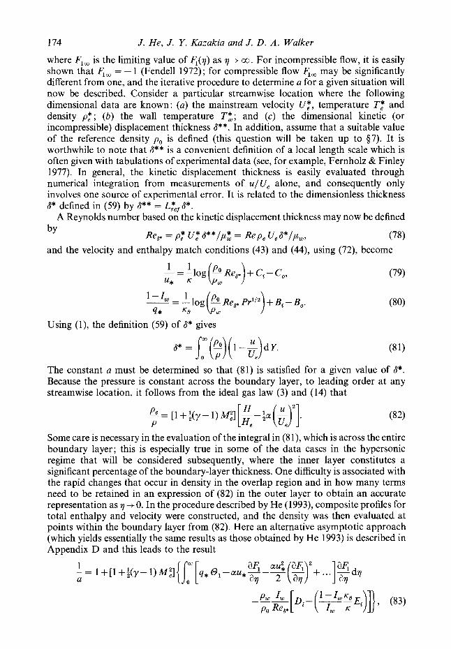
1 74 J. He, J . Y . Kazakia and J . D . A . Walker
where F,, is the limiting value of F,(7) as 7 --f 00. For incompressible flow, it is easily shown that F,, = - 1 (Fendell 1972); for compressible flow F,, may be significantly different from one, and the iterative procedure to determine a for a given situation will now be described. Consider a particular streamwise location where the following dimensional data are known: (a) the mainstream velocity U,*, temperature T,* and density p,*; (b) the wall temperature T:; and (c) the dimensional kinetic (or incompressible) displacement thickness a**. In addition, assume that a suitable value of the reference density po is defined (this question will be taken up to $7). It is worthwhile to note that S** is a convenient definition of a local length scale which is often given with tabulations of experimental data (see, for example, Fernholz & Finley 1977). In general, the kinetic displacement thickness is easily evaluated through numerical integration from measurements of u / U, alone, and consequently only involves one source of experimental error. It is related to the dimensionless thickness S* defined in (59) by S** = L* ref S* '
A Reynolds number based on the kinetic displacement thickness may now be defined
(78) Re,, = p,* U,* S**/p: = Rep, U, S*/pu,, by
and the velocity and enthalpy match conditions (43) and (44), using (72), become
Using (l), the definition (59) of S* gives
S* = / :e)( l -e)dY.
(79)
The constant a must be determined so that (81) is satisfied for a given value of S*. Because the pressure is constant across the boundary layer, to leading order at any streamwise location, it follows from the ideal gas law (3) and (14) that
= [l +f(y 1) @I [H,-2a(U,) H u 2 1. P
Some care is necessary in the evaluation of the integral in (8 I), which is across the entire boundary layer; this is especially true in some of the data cases in the hypersonic regime that will be considered subsequently, where the inner layer constitutes a significant percentage of the boundary-layer thickness. One difficulty is associated with the rapid changes that occur in density in the overlap region and in how many terms need to be retained in an expression of (82) in the outer layer to obtain an accurate representation as 7 + 0. In the procedure described by He (1993), composite profiles for total enthalpy and velocity were constructed, and the density was then evaluated at points within the boundary layer from (82). Here an alternative asymptotic approach (which yields essentially the same results as those obtained by He 1993) is described in Appendix D and this leads to the result
Asymptotic two-layer model for boundary layers 175
where D, and Ei are constants which can be calculated by numerical integration. Because 0, and Fi are implicit functions of a (cf. (73) and (74)), it follows that (83) constitutes a nonlinear equation for a which was solved iteratively according to the following procedure. Starting from an initial guess for a, solutions for Fi(7) and el(?), as well as C, and B,, were evaluated from (75) and (76). For a specified value of Kh, the profile O,(r) is based on an initial estimate of K ~ . With B, and Ci computed from the formulae in Appendix C (with T i = 110.2), K~ was then re-evaluated from (48). Since B, and Bi are implicit functions of K ~ , an inner iteration was carried out to determine a converged value of KO. Estimates of u* and q* were then obtained from (79) and (80). At this stage, the integrals in (83) were evaluated numerically using a trapezoidal rule on a non-uniform mesh that expanded with distance from the wall; typically 150 to 300 mesh points were found to give good accuracy. For a given value of a, (83) will not in general be satisfied and the value of a was then refined using an iteration based on the secant method. Note that for the extended Baldwin-Lomax model, a value of C,, = 1.733 was used; for this value of C,, identical results are obtained in the limit M,+O for both the extended Cebeci-Smith (1974) and Baldwin-Lomax (1978) models. In addition, for the extended Baldwin-Lomax (1978) model, a search was carried out - at any stage during the iterative procedure to find current estimates of nmaz and cnUz.
7. The reference condition The reference density po appears in the outer scale (72) and the matching conditions
(79) and (80), and a suitable choice for po and the reference temperature T, is important in determining the surface properties, as well as the physical extent of the outer region. As discussed in Q 1, the reference condition should be characteristic of the temperature in the near-wall region, and here two possible selections will be considered. First define the reference temperature as an average temperature across the wall layer according to
where Y: is some universal large value which is characteristic of the physical extent of the wall layer. It can be shown using (14), (19a) and (30a) that
T, = T, - T, {f(y- 1) M,2 u: A: - (1 +f(y - 1) @) q* B:}, (85)
to leading order, where the constants AT and B: are given by
A+ = Lloy' [ U+( Y+)I2 d Y+, Bl = jr' 0+( I") d Y+. Y: y :
Since U+ and O+ are known analytical functions (see Appendix C), AT and B: can be readily evaluated, and the results depend parametrically on the logarithmic-law constants K, Ci and K ~ , B,, as well as the value of Y: used.
Because the boundary between the inner and outer region is not distinct, it does not appear to be possible to define a unique value of Y: based on purely theoretical considerations. Since velocity and total enthalpy profile data in the wall layer are sparse and often of uncertain reliability, it was decided to establish a universal value of Y t through comparison with direct measurements of skin friction. Over the years, there has been considerable effort to improve the reliability of direct measurements of wall shear stress utilizing floating element balances (FEB). Currently, such data exist
176 J. He, J. Y. Kazakia and J . D. A . Walker
0.036
0.024
0’. % n
I x 3
v
0.012
36
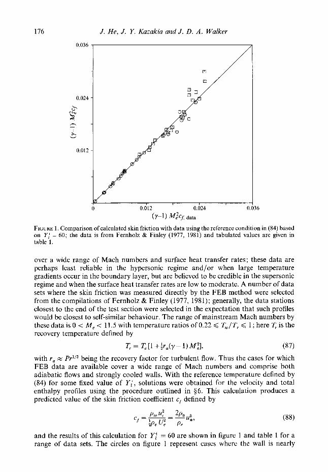
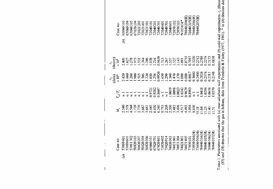
FIGURE 1. Comparison of calculated skin friction with data using the reference condition in (84) based on Y t = 60; the data is from Fernholz & Finley (1977, 1981) and tabulated values are given in table 1.
over a wide range of Mach numbers and surface heat transfer rates; these data are perhaps least reliable in the hypersonic regime and/or when large temperature gradients occur in the boundary layer, but are believed to be credible in the supersonic regime and when the surface heat transfer rates are low to moderate. A number of data sets where the skin friction was measured directly by the FEB method were selected from the compilations of Fernholz & Finley (1977, 1981); generally, the data stations closest to the end of the test section were selected in the expectation that such profiles would be closest to self-similar behaviour. The range of mainstream Mach numbers by these data is 0 < Me < 11.5 with temperature ratios of 0.22 < Tw/T, d 1 ; here T, is the recovery temperature defined by
T, = T,[1 + : r , ( y - l ) M f ] 7 (87)
with r , z Prli3 being the recovery factor for turbulent flow. Thus the cases for which FEB data are available cover a wide range of Mach numbers and comprise both adiabatic flows and strongly cooled walls. With the reference temperature defined by (84) for some fixed value of Y:, solutions were obtained for the velocity and total enthalpy profiles using the procedure outlined in $6. This calculation produces a predicted value of the skin friction coefficient cf defined by
and the results of this calculation for Y t = 60 are shown in figure 1 and table 1 for a range of data sets. The circles on figure 1 represent cases where the wall is nearly
Cas
e no
.
(a)
5301
0401
53
010
60 1
5301
1302
58
020
103
5802
0207
58
0203
04
58 0
20 3
06
6506
0 10
1 67
0207
01
6702
0801
73
0204
02
73 02
09 1
4 74
0203
03
7402
1 00
1 74
02 1
204
7402
1 80
1 74
02 1
805
7703
0101
73
050
304(
H)
73 05
0 50
4(H
) 78
040
104
(H)
7804
0 10
5(H
) 78
040
106(
H)
7804
0 10
7(H
)
Me
2.54
0 2.
578
4.54
4 1.
739
2.73
9 3.
667
3.68
1 2.
445
6.43
0 6.
340
0.79
3 2.
208
2.50
0 3.
483
3.49
6 4.
517
4.49
3 5.
994
9.83
0 10
.31
11.0
4 11
.23
11.4
0 11
.51
Twl T
, s
l
Zl
s
l
xl
Z
l
xl
z
l
0.97
21
0.92
82
0.86
07
zl
s
l
1.00
19
1.00
98
1.00
23
1.02
42
0.98
29
0.89
83
z51
xl
1.
0418
1.
0298
1.
0658
1.
0570
CJ
(dat
a)
2.42
0 1.
660
1.26
0 1.
900
1.51
5 1.
306
1.22
0 1.
030
1.25
6 0.
9920
1.
650
1.29
0 1.
560
1.47
0 1.
170
1.08
0 0.
880
0.80
17
0.30
40
0.24
00
0.28
26
0.25
78
0.23
1 1
0.21
48
x 10
3
Cf
(the
ory)
2.40
0 1.
627
1.27
8 1.
975
1.53
1 1.
344
1.24
6 1.
038
1.21
6 0.
9658
1.
713
1.26
7 1.
537
1.52
7 1.
143
1.09
1 0.
8755
0.
7997
0.
3220
0.
2212
0.
2789
0.
2279
0.
2173
0.
1838
x 10
3 C
ase
no.
(b)
6506
0103
65
060
104
6506
0 10
5 67
020
104
7202
1 20
3 72
021
401
7202
1 50
1 72
040
101
72 04
0 20
1 72
040
30 1
72 04
0 40
1 72
0405
01
72 04
0 60
1 72
050
102
7205
0 10
3 N
103
838*
78
0402
04(H
) 78
0402
05(H
) 78
040
206(
H)
78 0
4020
7(H
)
Me
4.91
5 4.
895
4.96
1 6.
490
4.85
7 4.
792
4.92
9 6.
210
6.39
0 6.
420
6.42
0 6.
500
6.50
0 7.
200
7.20
0 8.
013
11.1
7 11
.00
11.4
7 11
.42
CJ
(dat
a)
TW
IT
x lo
3
0.71
05
1.33
0 0.
5951
1.
410
0.52
28
1.48
0 0.
5253
1.
336
0.22
79
1.11
0 0.
2107
1.
720
0.22
42
1.30
0 0.
3330
1.
560
0.31
36
1.22
0 0.
4377
1.
230
0.41
94
1.25
0 0.
5082
1.
060
0.50
14
1.00
0 0.
4984
0.
850
0.47
64
0.80
0 0.
2970
0.
980
0.44
55
0.30
4 0.
4319
0.
288
0.43
64
0.24
8 0.
3808
0.
250
CJ
(the
ory)
1.31
9 1.
405
1.51
0 1.
388
1.17
3 1.
663
5 1.
239
2
1.20
0 1.
176
2 1.
258
$i 1.
019
2
0.94
9 5 3
0.79
7 0.
804
0
1.16
4 @
0.
333
0.29
3 0.
282
5
x 10
3
0.31
2 y B
.=. s. T
AB
LE
1. P
aram
eter
s as
soci
ated
with
(a
) nea
r-ad
iaba
tic
wal
l exp
erim
ents
and
(b
) col
d-w
all e
xper
imen
ts.
cr (
theo
ry)
is c
alcu
late
d fo
r Y
t =
60
in e
quat
ion
2 (8
5) a
nd (
H)
deno
tes
that
the
gas
is h
eliu
m;
data
fro
m F
ernh
olz
& F
inle
y (1
977,
198
1). *
in (
b) d
enot
es d
ata
from
Kus
soy
& H
orst
man
(19
91).
CL
4
4
178 J . He, J . Y. Kazakia and J. D . A . Walker
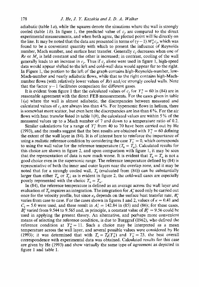
adiabatic (table 1 a), while the squares denote the situations where the wall is strongly cooled (table lb). In figure 1 , the predicted value of cf are compared to the direct experimental measurements, and when both agree, the plotted point will lie directly on the line. It may be noted that the data are presented in terms of (y - 1) Mz cf, which was found to be a convenient quantity with which to present the influence of Reynolds number, Mach number, and surface heat transfer. Generally cf decreases when one of Re or Me is held constant and the other is increased; in contrast, cooling of the wall generally leads to an increase in cr Thus if cf alone were used in figure 1, high-speed data would appear shifted to the left and cold-wall data would appear far to the right. In Figure 1, the portion to the left of the graph contains high-Reynolds-number, low- Mach-number and nearly adiabatic flows, while that to the right contains high-Mach- number flows (with relatively lower values of Re) and/or strongly cooled walls. Note that the factor y- 1 facilitates comparison for different gases.
It is evident from figure 1 that the calculated values of cf for Y: = 60 in (84) are in reasonable agreement with the direct FEB measurements. For the cases given in table l ( a ) where the wall is almost adiabatic, the discrepancies between measured and calculated values of cf are always less than 4 YO. For hypersonic flows in helium, there is somewhat more scatter, but even here the discrepancies are less than 6 YO. For the air flows with heat transfer listed in table 1 (b), the calculated values are within 5 YO of the measured values up to a Mach number of 7 and down to a temperature ratio of 0.2.
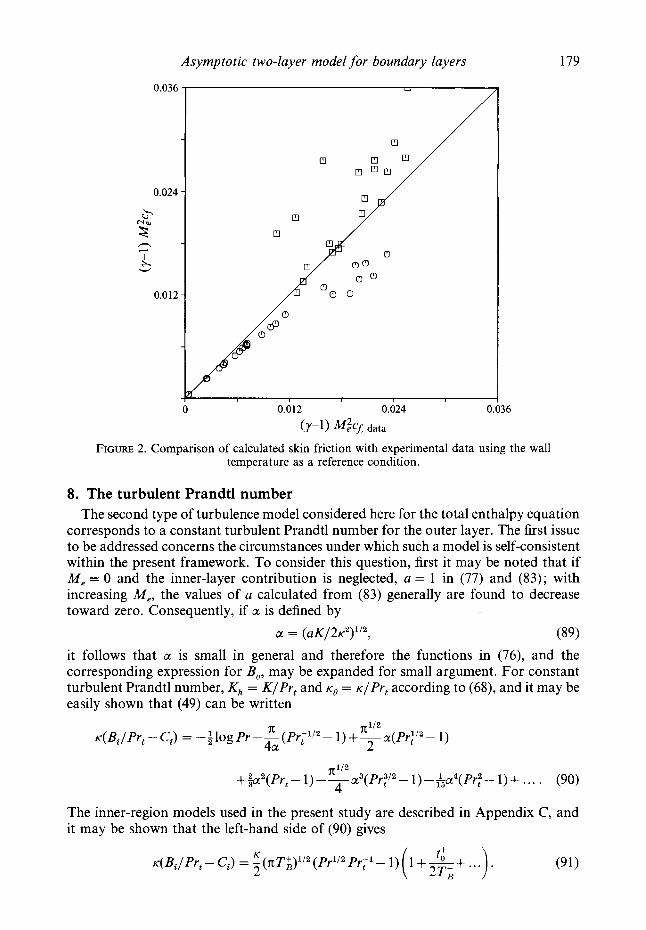
Similar calculations for a range of Y: from 40 to 70 have been carried out by He (1993), and the results suggest that the best results are obtained with YF = 60 defining the extent of the wall layer in (84). It is of interest here to reinforce the importance of using a realistic reference condition by considering the case Y: = 0, which corresponds to using the wall value for the reference temperature (T, = T,). Calculated results for this choice are shown in figure 2, and upon comparison with figure 1, it may be seen that the representation of data is now much worse. It is evident that To = T, is not a good choice even in the supersonic range. The reference temperature defined by (84) is representative of both the inner and outer layers near the overlap zone, and it may be noted that for a strongly cooled wall, T, (evaluated from (84)) can be substantially larger than either T, or T,; as is evident in figure 2, the cold-wall cases are especially poorly represented with the choice To = T,.
In (84), the reference temperature is defined as an average across the wall layer and evaluation of T, requires an integration. The integration for A: need only be carried out once for the velocity profile, but since K~ depends on the surface heat transfer rate, varies from case to case. For the cases shown in figures 1 and 2, values of K = 0.41 and Ci = 5.0 were used, and these result in A: = 142.84 in (85) and (86); for these cases, B: varied from 9.544 to 9.565 and, in principle, a constant value of = 9.56 could be used in applying the present theory. An alternative, and perhaps more convenient means of selecting the reference condition, is due to Burggraf (1962), who defined the reference condition at Y i = 11. Such a choice may be interpreted as a mean temperature across the wall layer, and several possible values were considered by He (1993); it was determined that with To = T,(Yi) and Y i = 23, the best overall correspondence with experimental data was obtained. Calculated results for this case are given by He (1993) and show virtually the same type of agreement as depicted in figure 1 and table 1.
Asymptotic two-layer model for boundary layers 179
FIGURE 2. Comparison of calculated skin friction with experimental data using the wall temperature as a reference condition.
8. The turbulent Prandtl number The second type of turbulence model considered here for the total enthalpy equation
corresponds to a constant turbulent Prandtl number for the outer layer. The first issue to be addressed concerns the circumstances under which such a model is self-consistent within the present framework. To consider this question, first it may be noted that if Me = 0 and the inner-layer contribution is neglected, a = 1 in (77) and (83); with increasing Me, the values of a calculated from (83) generally are found to decrease toward zero. Consequently, if a is defined by
a = ( a K / 2 K y , (89) it follows that a is small in general and therefore the functions in (76), and the corresponding expression for B,, may be expanded for small argument. For constant turbulent Prandtl number, Kh = K/Pr , and K* = K / P Y ~ according to (68), and it may be easily shown that (49) can be written
7c 7c1/2
4a 2 K(B,/Pr,-C,) = - ; logPr--(Pr; l 'z- l)+-a(Pri/2- 1)
7cl /2
4 +ga2(Pr,- l)--a3(Pr?/'- l)-&a4(Pr,2- 1)+ ... . (90)
The inner-region models used in the present study are described in Appendix C, and it may be shown that the left-hand side of (90) gives
K K(Bi/Prt - Ci) = - (n:T;)l/' (Pr'/' Pr-' t - 1)
2
180 J . He, J . Y . Kazakia and J . D. A. Walker
Consequently for a given model, Prandtl number, and value of a, (90) and (91) describe a nonlinear relation for Pr, which can easily be solved numerically. A rapidly convergent explicit series solution can be constructed of the form
where 2a2 16a3 3a4 16a5
3n nli2 15n P(a) = l+Ba+p+----- + ... ,
A - B 2a2 8a3 5a4 801' Q(a) =-a+-+------+ ... 2 7p x1/2 3 '
and A and B are constants given by
B = A + - l+- (nT;Pr)'/'. :( 2&)
(93 4
(93 b)
(94 b)
For given values of a, the turbulent Prandtl number may be evaluated directly from (92). In the incompressible limit M,+O a = 1 and a = 0.2235 (for K = 0.0168, K = 0.41); for the inner-layer parameters listed in (C 10) and Pr = 0.72, a value of Pr, = 0.872 may be calculated. This value compares favourably with the estimate of Pr, FZ 0.9 that is commonly used (see, for example, Fernholz & Finley 1980). It should be noted that (92) constitutes a theoretical prediction of Pr, and that in general Pr, cannot be specified arbitrarily if the outer-layer formulation is to remain self- consistent. In addition, it is worthwhile to emphasize that the present wall-layer formulation for total enthalpy is not a constant-Pr, model; this would seem to be desirable in general since measurements imply a significant variation in Pr, across the wall layer in subsonic flow (see, for example, Crawford & Kays 1980, p. 226).
For increasing Me, the results calculated for a from (83) indicate that a+O as Me --f co, and it is evident from (92) that in this limit Pr, + 1. Calculated values of a for Me lying in the range 0 < Me < 00 lie in the interval 0.872 < Pr, < 1 for P r = 0.72, and the results were closely curve-fitted with the following relation :
1 - exp ( -Po abl)
1 -exp(-Po) ' Pr, = 1-0.128 (95)
where Po = 1.6794 and PI = 0.4084. It is easily confirmed that there is a relatively slow variation for Pr, in the range 0.5 < a < 1, where the bulk of the supersonic data falls.
9. Calculated results
evaluated as follows. The inner variable Y+ is related to 7 by Profiles for velocity and total enthalpy across the entire boundary layer were
6* 7, y+ = Re PW
and with u* determined from (79), a composite profile for the velocity across the boundary layer is given by
Asymptotic two-layer model for boundary layers 181
Case no.
(a) 73020402* 58020207 74021 801* 65060 101 65060 105 72 090 402* 79030 103*(N) 72 040 20 1 72 040 60 1 71 030207(H) 71 030406(H) 73 050 504(H)
(b) f-1048 f-1548 f-2048 67010 105 67 0 10 204 72050 103 72 020 205 72 02 1 203 73 010 501
Me 0.793 2.739 4.517 4.886 4.801 7.780 8.788 6.390 6.500 6.686 6.686
2.160 2.170 2.140 5.970 6.040 7.200 4.823 4.857 4.742
10.31
TWIT Re,. a 1 139480 a 1 12255 1.0242 6945.5 0.9755 6699.7 0.5228 4987.8 0.7998 5686.5 0.3375 7518.1 0.3136 7667.2 0.5014 8435.7 0.9811 33813 0.9817 6580.2 z 1 17177
1.021 6450.5 1.475 5139.6 1.961 4831.9 0.4888 14120 0.4257 12083 0.4764 10433 0.9277 20730 0.2279 56517 1.0212 12352
PolPw 1.0109 1.1300 1.2730 1.2709 0.9670 1.3001 0.841 1 0.7468 0.9797 1.6187 1.4610 1.4627
1.1174 1.2995 1.428 1 0.9259 0.8672 0.9610 1.1697 0.5546 1.2397
a* 0.0308 0.0422 0.0507 0.0514 0.0460 0.0562 0.0461 0.0405 0.0458 0.0721 0.0617 0.0600
0.0439 0.0491 0.0525 0.0414 0.0409 0.045 1 0.0435 0.0275 0.0473
U*l,,P
0.0303 0.0421 0.0507 0.0514 0.0450 -
-
0.0399 0.0463
-
0.0443
0.0251 -
-
4* 0.0005 0.003 1 0.0037 0.0068 0.0286 0.0188 0.0382 0.0348 0.0297 0.0101 0.0086 0.0072
0.0021 0.0233
-0.0539 0.0274 0.0300 0.0305 0.0079 0.0261 0.0037
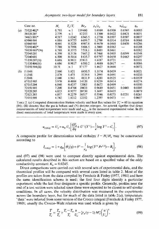
TABLE 2. (a) Computed dimensionless friction velocity and heat flux values for Y t = 60 in equation (84); (H) denotes that the gas is helium and (N) denotes nitrogen. An asterisk signifies that direct measurements of total temperature were made and u*leZp is the measured experimental value. In (b) direct measurements of total temperature were made in every case.
1 1 ucomp = ue+u* u, -+ U+(Y+)--log r+-ci . [: K
(97)
A composite profile for dimensionless total enthalpy I = H / H , may be constructed according to
and (97) and (98) were used to compare directly against experimental data. The calculated results described in this section are based on a specified value of the eddy conductivity constant Kh = 0.0245.
Direct comparisons were carried out with several sets of experimental data, and the theoretical profiles will be compared with several cases listed in table 2. Most of the profiles are taken from the data compiled by Fernholz & Finley (1977, 1981) and here the same identification scheme is used; the first four digits identify a particular experiment while the last four designate a specific profile. Generally, profiles near the end of a test section were selected since these were expected to be closest to self-similar conditions. In all cases, the velocity distribution was measured in the experiments across the boundary layer, but for much of the data listed in table 2(a), temperature ‘data’ were inferred from some version of the Crocco integral (Fernholz & Finley 1977, 1980); usually the Crocco-Walz relation was used which is given by
182 J
30
20
10
u+ 0
0
0
1 .o
1 .o
2 1.0 Tw
0.5
0
He, J . Y. Kazakia and J . D. A . Walker
73020402
71030406
I I I 1 1 1 1 1 1 1 I I 1 1 1 1 1 1 1 I I 1 1 1 1 1 1 1 I I "mil
10’ 102 103 104 Y+
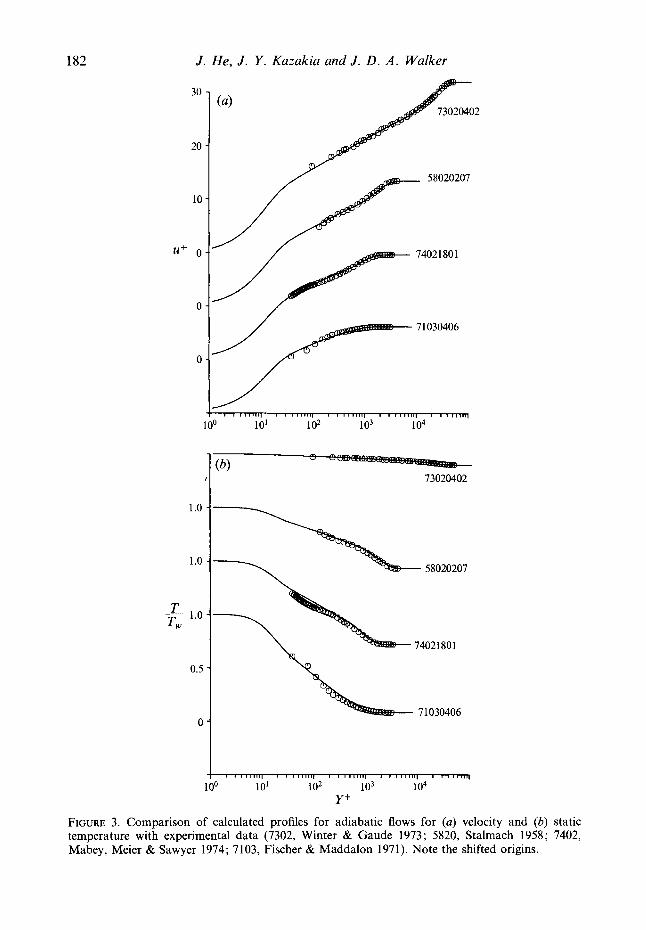
FIGURE 3. Comparison of calculated profiles for adiabatic flows for (a) velocity and (b) static temperature with experimental data (7302, Winter & Gaude 1973; 5820, Stalmach 1958; 7402, Mabey, Meier & Sawyer 1974; 7103, Fischer & Maddalon 1971). Note the shifted origins.
Asymptotic two-layer model for boundary layers
30
20
10
Uf 0
0
0
1 .o
1 .o
2. 1.0 T w
0.5
0
1
183
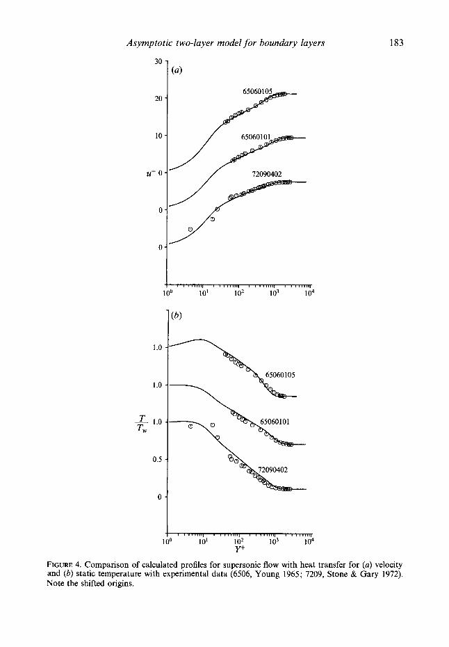
FIGURE 4. Comparison of calculated profiles for supersonic flow with heat transfer for (a) velocity and (b) static temperature with experimental data (6506, Young 1965; 7209, Stone & Gary 1972). Note the shifted origins.
184
30 7
20 -
10 -
U+ 0 -
0 -
0 -
(a)
I 8 #“““I ( 1 1 , 1 1 1 1 I ““W
100 10’ 102 103 104
1 .o
1 .o
1.0 TnJ
0.5
100 10’ 102 103 104 Y+
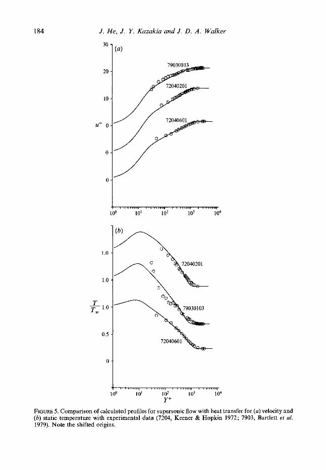
FIGURE 5. Comparison of calculated profiles for supersonic flow with heat transfer for (a) velocity and (b) static temperature with experimental data (7204, Keener & Hopkin 1972; 7903, Bartlett et al. 1979). Note the shifted origins.
Asymptotic two-layer model for boundary layers 185
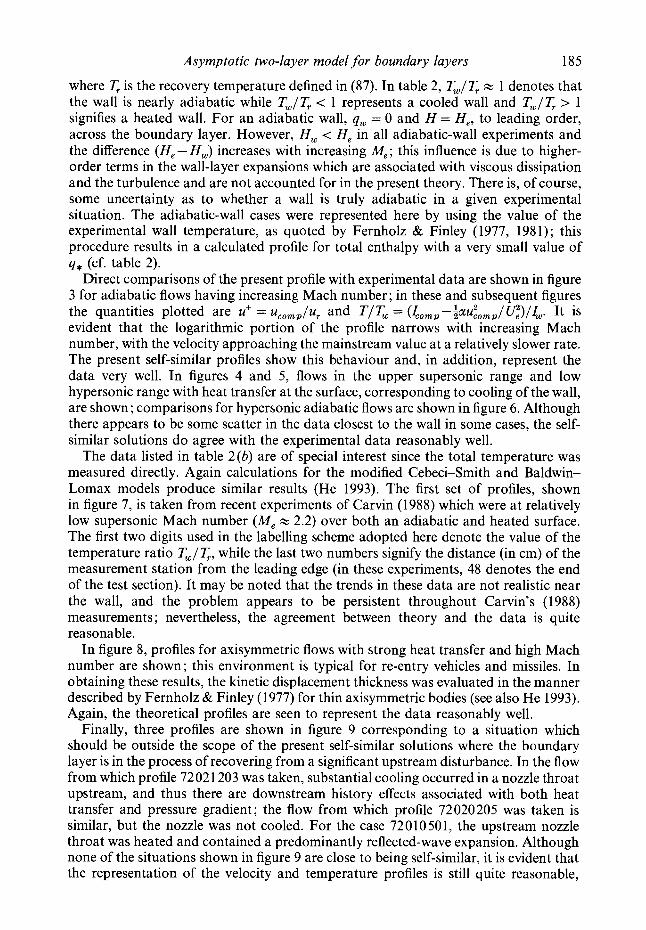
where T, is the recovery temperature defined in (87). In table 2, T,/T, x 1 denotes that the wall is nearly adiabatic while Tw/T, < 1 represents a cooled wall and Tw/T > 1 signifies a heated wall. For an adiabatic wall, qw = 0 and H = H,, to leading order, across the boundary layer. However, H, < H, in all adiabatic-wall experiments and the difference (He - H,) increases with increasing M,; this influence is due to higher- order terms in the wall-layer expansions which are associated with viscous dissipation and the turbulence and are not accounted for in the present theory. There is, of course, some uncertainty as to whether a wall is truly adiabatic in a given experimental situation. The adiabatic-wall cases were represented here by using the value of the experimental wall temperature, as quoted by Fernholz & Finley (1977, 1981); this procedure results in a calculated profile for total enthalpy with a very small value of q* (cf. table 2).
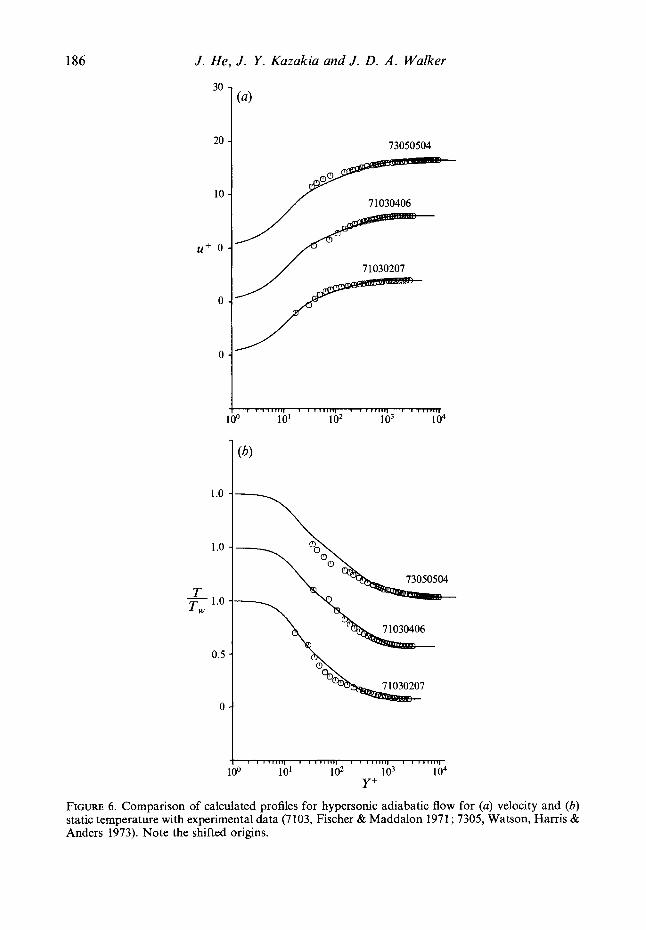
Direct comparisons of the present profile with experimental data are shown in figure 3 for adiabatic flows having increasing Mach number; in these and subsequent figures the quantities plotted are U+ = U , , , ~ / U , and T/T, = ( ~ o ~ p - ~ a u ~ o m p / ~ ) / ~ . It is evident that the logarithmic portion of the profile narrows with increasing Mach number, with the velocity approaching the mainstream value at a relatively slower rate. The present self-similar profiles show this behaviour and, in addition, represent the data very well. In figures 4 and 5, flows in the upper supersonic range and low hypersonic range with heat transfer at the surface, corresponding to cooling of the wall, are shown; comparisons for hypersonic adiabatic flows are shown in figure 6 . Although there appears to be some scatter in the data closest to the wall in some cases, the self- similar solutions do agree with the experimental data reasonably well.
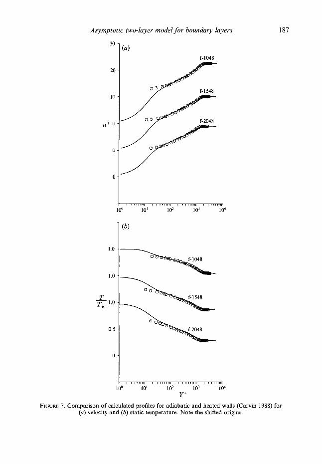
The data listed in table 2(b) are of special interest since the total temperature was measured directly. Again calculations for the modified Cebeci-Smith and Baldwin- Lomax models produce similar results (He 1993). The first set of profiles, shown in figure 7, is taken from recent experiments of Carvin (1988) which were at relatively low supersonic Mach number (Me x 2.2) over both an adiabatic and heated surface. The first two digits used in the labelling scheme adopted here denote the value of the temperature ratio T,/T,, while the last two numbers signify the distance (in cm) of the measurement station from the leading edge (in these experiments, 48 denotes the end of the test section). It may be noted that the trends in these data are not realistic near the wall, and the problem appears to be persistent throughout Carvin’s (1988) measurements ; nevertheless, the agreement between theory and the data is quite reasonable.
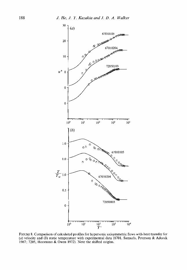
In figure 8, profiles for axisymmetric flows with strong heat transfer and high Mach number are shown; this environment is typical for re-entry vehicles and missiles. In obtaining these results, the kinetic displacement thickness was evaluated in the manner described by Fernholz & Finley (1977) for thin axisymmetric bodies (see also He 1993). Again, the theoretical profiles are seen to represent the data reasonably well.
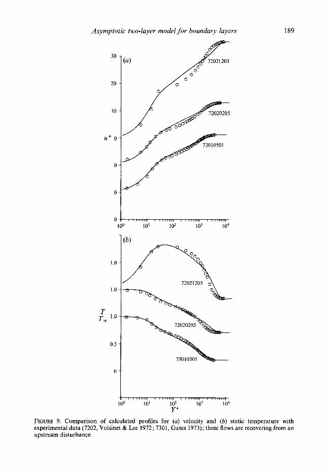
Finally, three profiles are shown in figure 9 corresponding to a situation which should be outside the scope of the present self-similar solutions where the boundary layer is in the process of recovering from a significant upstream disturbance. In the flow from which profile 72021 203 was taken, substantial cooling occurred in a nozzle throat upstream, and thus there are downstream history effects associated with both heat transfer and pressure gradient; the flow from which profile 72020205 was taken is similar, but the nozzle was not cooled. For the case 72010501, the upstream nozzle throat was heated and contained a predominantly reflected-wave expansion. Although none of the situations shown in figure 9 are close to being self-similar, it is evident that the representation of the velocity and temperature profiles is still quite reasonable,
186 J. He, J. Y. Kazakia and J. D. A . Walker
30
20
10
Uf 0
0
0
1 .o
1 .o
1.0 Tw
0.5
0
73050504
/ 71030406
/ 71030207
1 I I ~ ~ 1 ’ ~ ~ ) l 8 ~“ “ “ I 8 #‘@‘“‘I‘
101 1 02 103 104 Yf
FIGURE 6. Comparison of calculated profiles for hypersonic adiabatic flow for (a) velocity and (b) static temperature with experimental data (7103, Fischer & Maddalon 1971 ; 7305, Watson, Harris & Anders 1973). Note the shifted origins.
Asymptotic two-layer model for boundary layers
30 ] ( a ) f- 1048
1 .o
1 .o
1 .o 2 Tw
0.5
0
I /
187
I I I 1 1 1 1 1 1 1 I 0 ~~~~~~1 8 ~ ~ 1 ~ 1 1 1 0 10’ 102 103 104
Yf
FIGURE 7. Comparison of calculated profiles for adiabatic and heated walls (Carvin 1988) for (a) velocity and (b) static temperature. Note the shifted origins.
188 J . He, J. Y. Kazakia and J. D . A . Walker
20
10
u+ 0
0
1 .o
1 .o
2 T ,
0.5
0
8
72050103
FIGURE 8. Comparison of calculated profiles for hypersonic axisymmetric flows with heat transfer for (a) velocity and (b) static temperature with experimental data (6701, Samuels, Peterson & Adcock 1967; 7205, Horstman & Owen 1972). Note the shifted origins.
Asymptotic two-layer model for boundary layers 189
1 .o
1 .o
0.5
1 00 10' 102 103 104 Yf
FIGURE 9. Comparison of calculated profiles for (a) velocity and (b) static temperature with experimental data (7202, Voisinet & Lee 1972; 7301, Gates 1973); these flows are recovering from an upstream disturbance.
190 J. He, J. Y. Kazakia and J. D. A . Walker
I 73010501
0 100 10’ 1 02 103 104
Y+
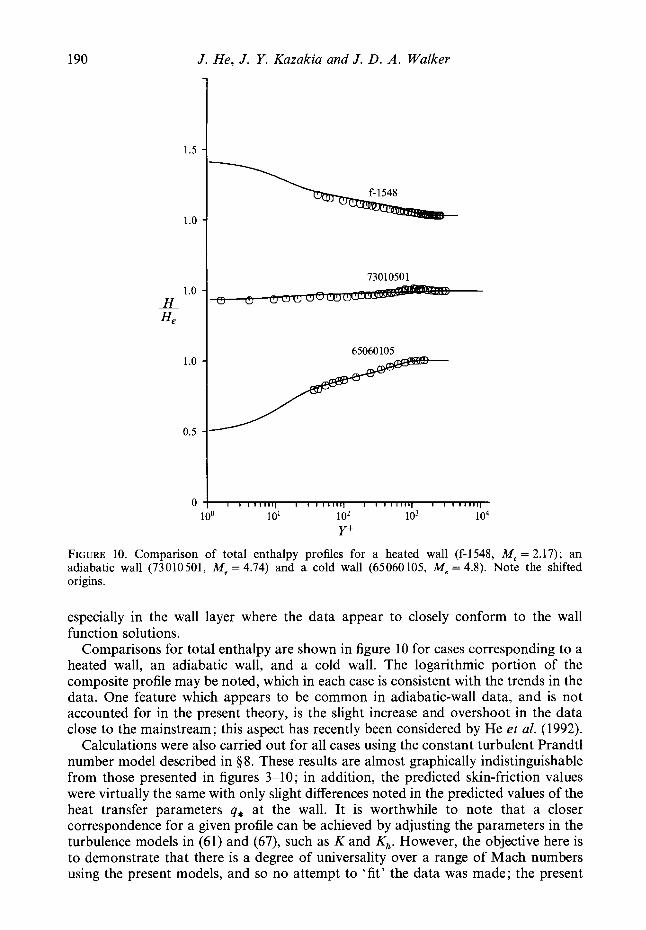
FIGURE 10. Comparison of total enthalpy profiles for a heated wall (f-1548, Me = 2.17); an adiabatic wall (73010501, M , = 4.74) and a cold wall (65060105, Me = 4.8). Note the shifted origins.
especially in the wall layer where the data appear to closely conform to the wall function solutions.
Comparisons for total enthalpy are shown in figure 10 for cases corresponding to a heated wall, an adiabatic wall, and a cold wall. The logarithmic portion of the composite profile may be noted, which in each case is consistent with the trends in the data. One feature which appears to be common in adiabatic-wall data, and is not accounted for in the present theory, is the slight increase and overshoot in the data close to the mainstream; this aspect has recently been considered by He et al. (1992).
Calculations were also carried out for all cases using the constant turbulent Prandtl number model described in 0 8. These results are almost graphically indistinguishable from those presented in figures 3-10; in addition, the predicted skin-friction values were virtually the same with only slight differences noted in the predicted values of the heat transfer parameters q* at the wall. It is worthwhile to note that a closer correspondence for a given profile can be achieved by adjusting the parameters in the turbulence models in (61) and (67), such as K and Kh. However, the objective here is to demonstrate that there is a degree of universality over a range of Mach numbers using the present models, and so no attempt to ‘fit’ the data was made; the present
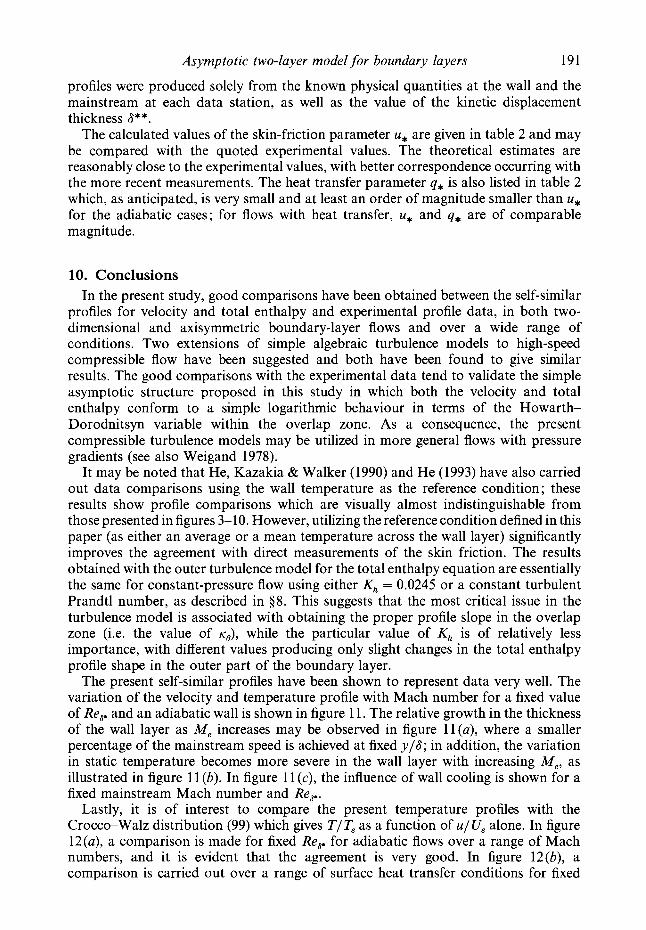
Asymptotic two-layer model for boundary layers 191
profiles were produced solely from the known physical quantities at the wall and the mainstream at each data station, as well as the value of the kinetic displacement thickness a**.
The calculated values of the skin-friction parameter u* are given in table 2 and may be compared with the quoted experimental values. The theoretical estimates are reasonably close to the experimental values, with better correspondence occurring with the more recent measurements. The heat transfer parameter q* is also listed in table 2 which, as anticipated, is very small and at least an order of magnitude smaller than u* for the adiabatic cases; for flows with heat transfer, u* and q* are of comparable magnitude.
10. Conclusions In the present study, good comparisons have been obtained between the self-similar
profiles for velocity and total enthalpy and experimental profile data, in both two- dimensional and axisymmetric boundary-layer flows and over a wide range of conditions. Two extensions of simple algebraic turbulence models to high-speed compressible flow have been suggested and both have been found to give similar results. The good comparisons with the experimental data tend to validate the simple asymptotic structure proposed in this study in which both the velocity and total enthalpy conform to a simple logarithmic behaviour in terms of the Howarth- Dorodnitsyn variable within the overlap zone. As a consequence, the present compressible turbulence models may be utilized in more general flows with pressure gradients (see also Weigand 1978).
It may be noted that He, Kazakia & Walker (1990) and He (1993) have also carried out data comparisons using the wall temperature as the reference condition; these results show profile comparisons which are visually almost indistinguishable from those presented in figures 3-10. However, utilizing the reference condition defined in this paper (as either an average or a mean temperature across the wall layer) significantly improves the agreement with direct measurements of the skin friction. The results obtained with the outer turbulence model for the total enthalpy equation are essentially the same for constant-pressure flow using either Kh = 0.0245 or a constant turbulent Prandtl number, as described in $8. This suggests that the most critical issue in the turbulence model is associated with obtaining the proper profile slope in the overlap zone (i.e. the value of KJ, while the particular value of Kh is of relatively less importance, with different values producing only slight changes in the total enthalpy profile shape in the outer part of the boundary layer.
The present self-similar profiles have been shown to represent data very well. The variation of the velocity and temperature profile with Mach number for a fixed value of Re,, and an adiabatic wall is shown in figure 1 1. The relative growth in the thickness of the wall layer as Me increases may be observed in figure ll(a), where a smaller percentage of the mainstream speed is achieved at fixed y / 6 ; in addition, the variation in static temperature becomes more severe in the wall layer with increasing Me, as illustrated in figure 11 (b). In figure 11 (c), the influence of wall cooling is shown for a fixed mainstream Mach number and Re,,.
Lastly, it is of interest to compare the present temperature profiles with the Crocco-Walz distribution (99) which gives T/T, as a function of u/Ue alone. In figure 12(a), a comparison is made for fixed Re,, for adiabatic flows over a range of Mach numbers, and it is evident that the agreement is very good. In figure 12(b), a comparison is carried out over a range of surface heat transfer conditions for fixed
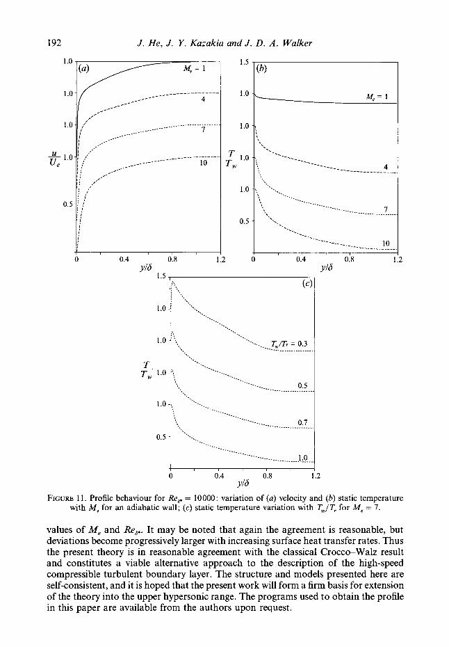
192 J . He, J, Y. Kazakia and J. D. A . Walker
FIGURE 11. Profile behaviour for Re,, = 10000: variation of (a) velocity and (b) static temperature with M e for an adiabatic wall; (c) static temperature variation with Tw/T, for Me = 7.
values of Me and Re,,. It may be noted that again the agreement is reasonable, but deviations become progressively larger with increasing surface heat transfer rates. Thus the present theory is in reasonable agreement with the classical Crocco-Walz result and constitutes a viable alternative approach to the description of the high-speed compressible turbulent boundary layer. The structure and models presented here are self-consistent, and it is hoped that the present work will form a firm basis for extension of the theory into the upper hypersonic range. The programs used to obtain the profile in this paper are available from the authors upon request.
Asymptotic two-layer model for boundary layers 193
1 .o
1 .o
1.0
T 1.0 Tw
1.0
0.5
0
1 .a
1 .a
1 .o
0.5
0
2.0
0.5
0.3
0 lbl i b 2 id3 1G4
Y+
FIGURE 12. Comparison of CroccwWalz (-----) relation (99) for static temperature with the present theory (-) for Re, = 10000; (a) variation with Me in adiabatic flow and (b) variation with TWIT for Me = 5.
This work was supported by NASA under Grant No. NAG-1-832 and AFOSR under Grant No. 89-0487.
Appendix A Here it is argued that the Chapman-Rubesin law pp = pw pw is valid to leading order
in the turbulent wall layer in the limit of large Reynolds number. At any streamwise location in the boundary layer, p is independent of n to leading order, and thus p T = pw Tw for any fixed streamwise location s. From (14),
According to (19a), (30a), and (A l), T z Tw in the wall layer to leading order. Consequently, if the variation of viscosity is given by either the Sutherland law or, even for a power law such as p K T" (Stewartson 1964), it follows that
2!5= 1 +O(u*), P W Y W
to leading order in the wall.
Appendix B
9' denote a dimensionless rate of total energy loss (with respect to pFef In this Appendix, the physical significance of the terms in (27) will be described. Let
T:ef)
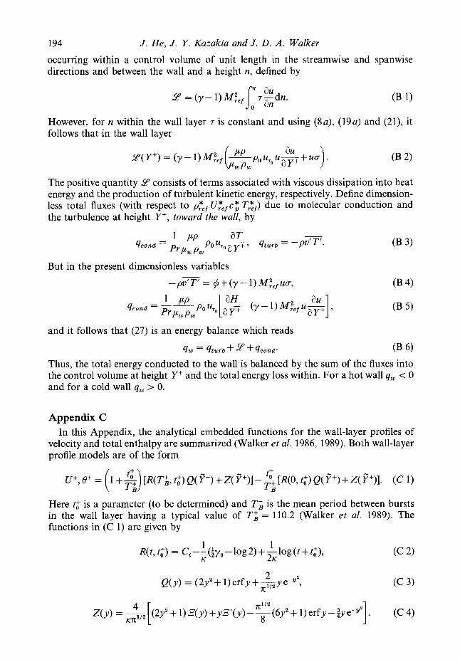
194 J . He, J . Y. Kazakia and J . D. A . Walker
occurring within a control volume of unit length in the streamwise and spanwise directions and between the wall and a height n, defined by
2 = (7- l)M$,, s: 7-dn. :: (B 1)
However, for n within the wall layer 7 is constant and using (8a), (19a) and (21), it follows that in the wall layer
The positive quantity 2 consists of terms associated with viscous dissipation into heat energy and the production of turbulent kinetic energy, respectively. Define dimension- less total fluxes (with respect to p:ef UFefc; T$f) due to molecular conduction and the turbulence at height Y+, toward the wall, by
But in the present dimensionless variables -
-pv'T' = #+(7- l ) M $ e f ~ ~ ,
and it follows that (27) is an energy balance which reads
qw = qturb+2+qco%d' (B 6)
Thus, the total energy conducted to the wall is balanced by the sum of the fluxes into the control volume at height Y+ and the total energy loss within. For a hot wall qw < 0 and for a cold wall qw > 0.
Appendix C In this Appendix, the analytical embedded functions for the wall-layer profiles of
velocity and total enthalpy are summarized (Walker et al. 1986, 1989). Both wall-layer profile models are of the form
U+,@ = (1 +&)[R(Ti , t;)Q(?)+Z(p+)]-L[R(O, ti)Q(?)+Z(?)]. (C 1)
Here t i is a parameter (to be determined) and T i is the mean period between bursts in the wall layer having a typical value of T i = 110.2 (Walker et al. 1989). The functions in (C 1) are given by
t+
T i
(C 2) 1 1
R(t, t i ) = ci --(+yo - log 2) +-log ( t + t i ) , K 2K
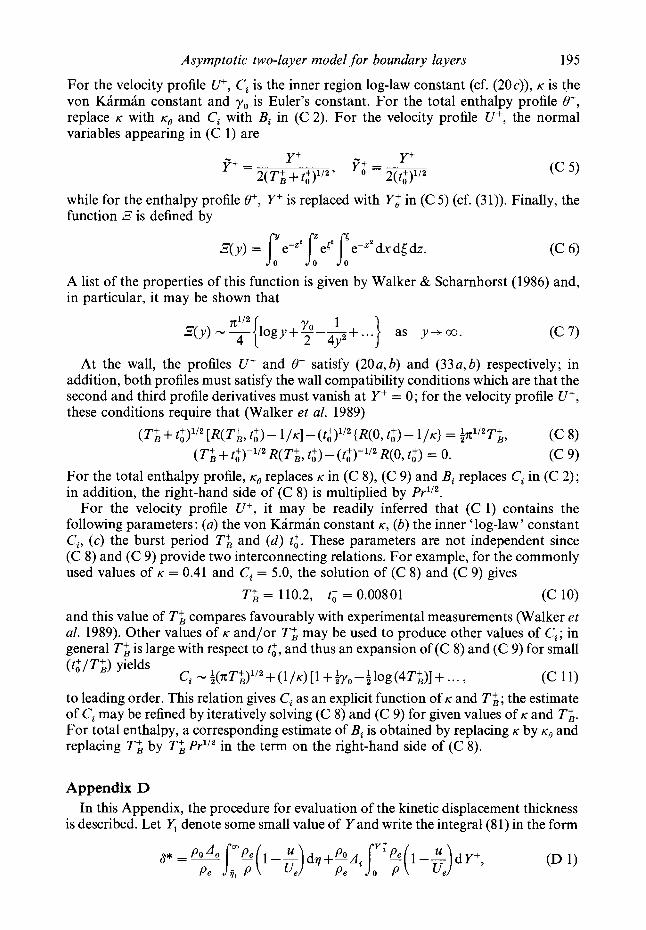
Asymptotic two-layer model for boundary layers 195
For the velocity profile U+, Ci is the inner region log-law constant (cf. ( ~ O C ) ) , K is the von Karman constant and yo is Euler's constant. For the total enthalpy profile Of, replace K with K~ and Ci with B, in ( C 2 ) . For the velocity profile U+, the normal variables appearing in (C 1 ) are
- Y+ - Y + y+ = +--
2( T i + ' yo - 2(t,+)lI2
while for the enthalpy profile O+, Y+ is replaced with Y,f in (C 5 ) (cf. (31)). Finally, the function B is defined by
E( y ) = e-" [ ec2 e-"' dx d( dz. (C 6 ) 0 0 0
A list of the properties of this function is given by Walker & Scharnhorst (1986) and, in particular, it may be shown that
At the wall, the profiles U + and O+ satisfy (20a,b) and (33a,b) respectively; in addition, both profiles must satisfy the wall compatibility conditions which are that the second and third profile derivatives must vanish at Y + = 0; for the velocity profile U+, these conditions require that (Walker et al. 1989)
(T;+t i )1 /2[R(TL, t:)- 1/K]-(ti)1'2{R(0, t:)- I / K } = $i?"TL, (C 8 ) (C 9) ( T i + R(Ti , t i ) -(t:)-'I2 R(0, t i ) = 0.
For the total enthalpy profile, K~ replaces K in (C 8) , (C 9) and B, replaces C, in (C 2) ; in addition, the right-hand side of (C 8 ) is multiplied by Pr'/2.
For the velocity profile U+, it may be readily inferred that (C 1) contains the following parameters : (a) the von Karman constant K, (b) the inner 'log-law ' constant C,, (c) the burst period T i and ( d ) t i . These parameters are not independent since (C 8 ) and (C 9) provide two interconnecting relations. For example, for the commonly used values of K = 0.41 and Ci = 5.0, the solution of (C 8 ) and (C 9) gives
and this value of T i compares favourably with experimental measurements (Walker et al. 1989). Other values of K and/or T i may be used to produce other values of Ci; in general TL is large with respect to t i , and thus an expansion of (C 8 ) and (C 9) for small
T i = 110.2, t i = 0.00801 (C 10)
to leading order. This relation gives C, as an explicit function of K and T i ; the estimate of Ci may be refined by iteratively solving (C 8 ) and (C 9) for given values of K and T i . For total enthalpy, a corresponding estimate of B, is obtained by replacing K by K~ and replacing T i by T i Pr1/2 in the term on the right-hand side of (C 8).
Appendix D
is described. Let In this Appendix, the procedure for evaluation of the kinetic displacement thickness
denote some small value of Y and write the integral (81) in the form
6* = A " 6. t (1 - 6) dy + A, loy' t ( 1 -6) d Y+,
Pl?
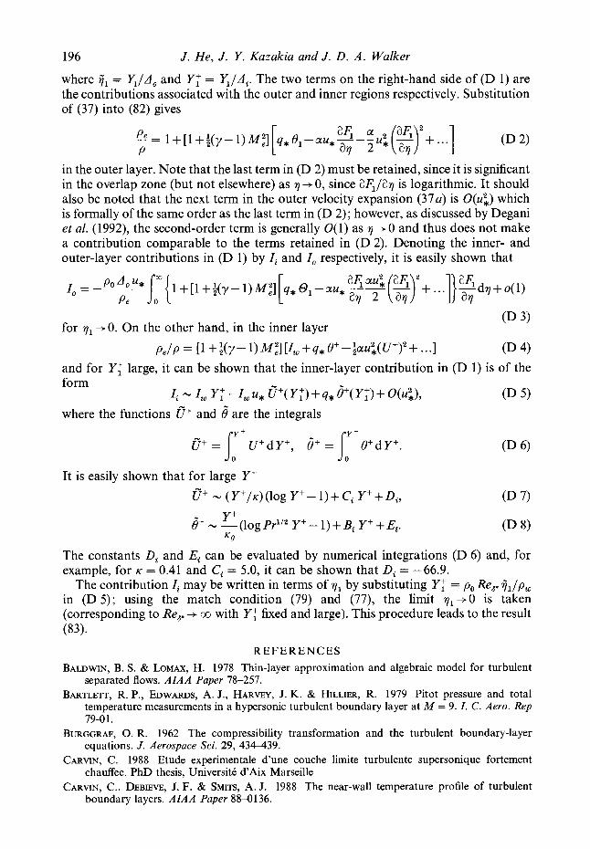
196 J . He, J . Y. Kazakia and J. D . A . Walker
where f 1 = & / A , and Y: = YJA, . The two terms on the right-hand side of (D 1) are the contributions associated with the outer and inner regions respectively. Substitution of (37) into (82) gives
aF, a 6 = 1 + [ 1 + f(y - 1) A43 q* 8, - au, u: gy + . . .] (D 2) P a7 2
in the outer layer. Note that the last term in (D 2) must be retained, since it is significant in the overlap zone (but not elsewhere) as 7 + 0, since afJa7 is logarithmic. It should also be noted that the next term in the outer velocity expansion (37a) is O(u2,) which is formally of the same order as the last term in (D 2); however, as discussed by Degani et al. (1992), the second-order term is generally O( 1) as 7 + 0 and thus does not make a contribution comparable to the terms retained in (D 2). Denoting the inner- and outer-layer contributions in (D 1) by I, and I, respectively, it is easily shown that
(D 3)
(D 4)
for v1 + 0. On the other hand, in the inner layer
and for Y: large, it can be shown that the inner-layer contribution in (D 1) is of the pe/p = [l +a(?- 1)M:][I,+g*8+-fau;(U+)2+...]
form I, - I , Y: -I, u* 6+( Y:) + q* S+( Y:) + O(ui),
where the functions 6+ and 6 are the integrals
It is easily shown that for large Y i
(log Pr'I2 Y+ - 1) + B, Y+ + Ei. e"+ N - (D 8) Y+
K8
The constants Di and E, can be evaluated by numerical integrations (D 6) and, for example, for K = 0.41 and C, = 5.0, it can be shown that Di = -66.9.
The contribution Ii may be written in terms of 7, by substituting Y: = po Re,, fJp, in (D 5 ) ; using the match condition (79) and (77), the limit r1+0 is taken (corresponding to Re,, + co with Y: fixed and large). This procedure leads to the result (83).
R E F E R E N C E S
BALDWIN, B. S. & LOMAX, H. 1978 Thin-layer approximation and algebraic model for turbulent separated flows. AIAA Paper 78-257.
BARTLETT, R. P., EDWARDS, A. J., HARVEY, J. K. & HILLIER, R. 1979 Pitot pressure and total temperature measurements in a hypersonic turbulent boundary layer at M = 9. I. C. Aero. Rep
BURGGRAF, 0. R. 1962 The compressibility transformation and the turbulent boundary-layer
CARVIN, C. 1988 Etude experimentale d'une couche limite turbulente supersonique fortement
CARVIN, C., DEBIEVE, J. F. & SMITS, A. J. 1988 The near-wall temperature profile of turbulent
79-0 1.
equations. J . Aerospace Sci. 29, 434-439.
chauffee. PhD thesis, UniversitC d'Aix Marseille
boundary layers. AZAA Paper 88-0136.
Asymptotic two-layer model for boundary layers 197
CEBECI, T. & SMITH, A. M. 0. 1974 Analysis of Turbulent Boundary Layers. Academic. COLES, D. 1964 The turbulent boundary layer in a compressible fluid. Adv. Appl. Mech. 1, 1-51. CRAWFORD, M. E. & KAYS, W. M. 1980 Convective Heat and Mass Transfer. McGraw-Hill. CROCCO, L. 1963 Transformations of the compressible turbulent boundary layer with heat exchange.
DEGANI, A. T., SMITH, F. T. & WALKER, J. D. A. 1992 The three-dimensional turbulent boundary
DEGANI, A. T., SMITH, F. T. & WALKER, J. D. A. 1993 The structure of a three-dimensional
DEGANI, A. T. & WALKER, J. D. A. 1993 Computation of attached three-dimensional turbulent
DEGANI, A. T., WALKER, J . D. A., ERSOY, S. & POWER, G. 1991 On the application of algebraic
FENDELL, F. E. 1972 Singular perturbation and turbulent shear flow near walls. J . Astro. Sci. 20,
FERNHOLZ, H. H. & FINLEY, P. J. 1977 A critical compilation of compressible turbulent boundary layer data. AGARD-AG-223.
FERNHOLZ, H. H. & FINLEY, P. J. 1980 A critical commentary on mean flow data for two- dimensional compressible turbulent boundary layers. AGARD-AG-253.
FERNHOLZ, H. H. & FINLEY, P. J. 1981 A further compilation of compressible boundary layer data with a survey of turbulence data. AGARD-AG-263.
FISCHER, M. C. & MADDALON, D. V. 1971 Experimental laminar, transitional and turbulent boundary-layer profiles on a wedge at local Mach number 6.5 and comparisons with theory.
GATES, D. F. 1973 Measurements of upstream history effects in compressible turbulent boundary layers. NOL T R 73-152.
HE, J. 1993 Asymptotic structure of supersonic turbulent boundary layers. PhD thesis, Lehigh University, Bethlehem, PA.
HE, J., KAZAKIA, J. Y. & WALKER, J. D. A. 1990 Embedded function methods for supersonic boundary layers. AIAA Paper 90-0306.
HE, J . , KAZAKIA, J. Y., RUBAN, A. I. & WALKER, J. D. A. 1992 An algebraic model for dissipation in supersonic boundary layers. AZAA Paper 92-03 11.
HE, J. & WALKER, J. D. A. 1995 A note on the Baldwin-Lomax model. Trans. ASME I: J. Fluids Engng (in press).
HORSTMAN, C. C. & OWEN, F. K. 1972 Turbulent properties of a compressible boundary layer. AIAA J. 10, 1418.
JOHNSON, J. A. & KING, L. S. 1985 A mathematically simple turbulence closure model for attached and separated turbulent boundary layers. AZAA J . 23, 1684-1692.
KEENER, E. R. & HOPKINS, E. J. 1972 Turbulent boundary layer profiles on a nonadiabatic flat plate at Mach number 6.5. NASA TN D-6907.
KEYES, F. G. 1952 The heat conductivity, viscosity, specific heat and Prandtl number for thirteen gases. Project Squid TR 37. MIT, Cambridge, MA.
KLINE, S. J., CANTWELL, B. J. & LILLEY, G. M. 1981 The 198041 AFOSR-HTTM-Stanford Conference on Complex Turbulent Flows: Comparison of Computation and Experiments, vols. 1-111. Thermosciences Division, Stanford University.
K u s s o ~ , I . & HORSTMAN, K. C. 1991 Documentation of two- and three-dimensional shock- wave/turbulent boundary-layer interaction flows at Mach 8.2. NASA Tech. Memo. 103838.
MABEY, D. G., MEIER, H. U. & SAWYER, K. G. 1974 Experimental and theoretical studies of the boundary layer on a flat plate at Mach numbers from 2.5 to 4.5. RAEITR 74127.
MAISE, G. & MCDONALD, H. 1968 Mixing length and kinematic eddy viscosity in a compressible boundary layer. AZAA J . 6, 73-80.
MELLOR, G. L. 1972 The large Reynolds number asymptotic theory of turbulent boundary layers. Znt. J . Engng Sci 10, 851-873.
MELLOR, G. L. & GIBSON, D. M. 1966 Equilibrium turbulent boundary layers. J . Fluid Mech. 24,
AIAA J . 1, 2723-2731.
layer near a plane of symmetry. J . Fluid Mech. 234, 329-360.
turbulent boundary layer. J. Fluid Mech. 250, 43-68.
boundary. J . Comput. Phys. 109, 202-214.
turbulence models to high Mach number flows. AZAA Paper 90-0616.
129- 1 65.
NASA TN D-6462.
225-253.
198 J. He, J. Y. Kazakia and J. D . A . Walker
ROTTA, J. C. 1960 Turbulent boundary layers with heat transfer in compressible flow. AGARD Rep. 251.
SAMUELS, R. D., PETERSON, J. B. & ADCOCK, J. B. 1967 Experimental investigation of the turbulent boundary layer at a Mach number of 6 with heat transfer at high Reynolds numbers. NASA TN
SMITH, C. R., WALKER, J. D. A., HAIDARI, A. H. & SOBRUN, U. 1991 On the dynamics of near-wall turbulence. Phil. Trans. R . SOC. Lond. A 336, 131-175.
STALMACH, C. J. 1958 Experimental investigation of the surface impact probe method of measuring local skin friction at supersonic speeds. University of Texas DRL-410, C F 2675.
STEWARTSON, K. 1964 The Theory of Laminar Boundary Layers in Compressible Fluids. Oxford University Press.
STONE, D. R. & GARY, A. M. 1972 Discrete sonic jets used as boundary layer trips at Mach numbers of 6 and 8.5. NASA TN D-6802.
TALCOTT, N. A. & KUMAR, A. 1985 Two-dimensional viscous simulation of inlet/diffuser flows with terminal shocks. J . Propulsion 1, 103-108.
VAN DRIEST, E. R. 1951 Turbulent boundary layer in compressible fluids. J . Aero. Sci. 18, 145-161. VIEGAS, J. R., RUBESIN, M. W. & HORSTMAN, C. C. 1985 On the use of wall functions as boundary
conditions for two-dimensional separated compressible flows. AZAA Paper 85-0180. VOISINET, L. P. & LEE, R. E. 1972 Measurements of a Mach 4.9 zero pressure gradient turbulent
boundary layer with heat transfer. NOL TR 72-232. WALKER, J. D. A,, ABBOTT, D. E., SCHARNHORST, R. K. & WEIGAND, G. G. 1989 Wall layer model
for the velocity profile in turbulent flows. AZAA J. 27, 14&149. WALKER, J. D. A. & SCHARNHORST, R. K. 1986 The 8 function. Dept Mechanical Engineering and
Mechanics, Lehigh University, Bethlehem, Pennsylvania, Rep. FM-9; Air Force Office of Scientific Research, AFOSR-TR-1715TR (available NTIS-AD-A188680).
WALKER, J. D. A., SCHARNHORST, R. K. & WEIGAND, G. G. 1986 Wall layer models for the calculation of velocity and heat transfer in turbulent boundary layers. AZAA Paper 86-0213.
WALKER, J. D. A., WERLE, M. J. & ECE, M. C. 1987 An embedded function approach for turbulent flow prediction. AZAA J. 29, 181g1818.
WATSON, R. D., HARRIS, J. E. & ANDERS, J. B. 1973 Measurements in a transitional/turbulent Mach 10 boundary layer at high Reynolds numbers. AZAA Paper 73-165.
WEIGAND, G. G. 1978 Forced convection in a two-dimensional nominally steady turbulent boundary layer. PhD thesis, Purdue University.
WHITE, F. M. 1992 Viscous Fluid Flow. McGraw-Hill. WHITE, F. M. & CHRISTOPH, G. H. 1972 Simple theory for two-dimensional compressible turbulent
boundary layer. Trans. ASME J. Basic Engng 94, 636642. WINTER, K. G. & GAUDET, L. 1973 Turbulent boundary-layer studies at high Reynolds numbers at
Mach numbers between 0.2 and 2.8. ARC R&M 3712. YOUNG, F. L. 1965 Experimental investigation of the effects of surface roughness on compressible
turbulent boundary layer skin friction and heat transfer. University of Texas Rep. DRL-532, AD 621 085.
D-3858.
Related Documents