An assessment of the acoustic survey technique, RoxAnn, as a means of mapping seabed habitat

Page 1

ICES Journal of Marine Science, 54: 939–959. 1997

An assessment of the acoustic survey technique, RoxAnn, as ameans of mapping seabed habitat

Simon P. R. Greenstreet, Ian D. Tuck,Gavin N. Grewar, Eric Armstrong, David G. Reid,and Peter J. Wright

Greenstreet, S. P. R., Tuck, I. D., Grewar, G. N., Armstrong, F., Reid, D. G., andWright, P. J. 1997. An assessment of the acoustic survey technique, RoxAnn, as ameans of mapping seabed habitat. – ICES Journal of Marine Science, 54: 939–959.

RoxAnn acoustic surveys of the inner Moray Firth, undertaken in September/October1995 and January 1996, were used to map seabed habitat on the basis of two sedimentcharacteristics, ‘‘roughness’’ (E1) and ‘‘hardness’’ (E2). The traditional analyticalmethod of fitting a ‘‘box pattern’’ to E1 vs. E2 scatter plots was compared with a moreobjective method using False Colour Composite Image (FCCI) and cluster analysis.Although both methods produced similar maps, the latter provided greater betweensurvey consistency. Six to seven sediment types were indicated by RoxAnn, howeverordination analysis of sediment samples indicated that some of the FCCI clusterscould not be separated on the basis of their particle size distributions. This may havebeen due to a degree of depth sensitivity, but it is also possible that RoxAnn wasresponding to other physical or biotic seabed features other than just particle size.After combining RoxAnn FCCI clusters where ground-truthing grab samples hadshown the particle size distributions to be similar, it was evident that RoxAnn coulddistinguish three main sediment habitats with certainty. On this basis, the RoxAnnderived maps compared well with maps obtained from British Geological Survey data.Finally we examined the distributions of four flatfish species to determine whetherthese were in any way related to the different sediment habitats identified by RoxAnn.

Key words: RoxAnn, seabed sediment habitat, mapping, acoustic survey, False ColourComposite Image analysis, habitat selection.

Received 7 October 1996; accepted 9 January 1997.

S. P. R. Greenstreet, I. D. Tuck, G. N. Grewar, F. Armstrong, D. G. Reid, and P. J.Wright: S.O.A.E.F.D., Marine Laboratory, PO Box 101, Victoria Road, Aberdeen,AB11 9DB, UK. Correspondence to S. P. R. Greenstreet: tel: +441224295417; fax:+441224295511; email: [email protected]

Introd

Habitatrespect t1973; CTurner,species leinstanceto the d1970; Mcharacteimportanof a paRand, 1and Houdeterminareas (M

1hi

wihuetesto, whon

1054–313

by guest on July 22, 2011icesjm

s.oxfordjournals.orgD

ownloaded from

uction

selection can have important consequences witho the fitness of individuals (King and Dawson,atchpole, 1974; Holbrook and Schmitt, 1988;1996), and ultimately affects fitness at thevel (Werner, 1977; Rosenzweig, 1995). In manys the distribution of predators is directly relatedistribution of their prey (Fretwell and Lucas,ilinski and Parker, 1991). However, physicalristics of the environmental also have an

Keast,miningfore anvalueSuc

conseqwherein Huscarceseabedrelied

t role to play in determining where individualsrticular species choose to live (Wecker, 1963;964; Douglass, 1976; Partridge, 1978; Carboneston, 1994). Habitat variability is a key factor ining the number of species living within definedacArthur and MacArthur, 1961; Eadie and

(e.g. BGDuinevesurveysand timesystem (Macoustic

9/97/050939+21 $25.00/0/jm970220

984; Huston, 1994; Rosenzweig, 1995). Deter-abitat variability in particular regions is there-mportant aspect in the assessment of a region’sth respect to species conservation.assessments are more easily carried out, andntly are more common and more detailed,rrestrial landscapes are concerned (see examplesn, 1994). They are particularly difficult, andith respect to marine habitats. Assessment ofabitat variation, for example, has traditionalyintensive sediment grab sampling programmes

S, 1984, 1987; Basford and Eleftheriou, 1988;ld et al., 1991; Heip et al., 1992) or diving(Hiscock, 1990), both of which are expensiveconsuming. The recently developed RoxAnnarine Microsystems Ltd, Ireland) provides analternative to these labour and time intensive

Page 2

technto beperio1993;techndetecsive oSchwRo

first aof theof threprewholeof sea1993)scatteclustea ‘‘bomaximassumdefinenumbthatrepresuchthis aThesea parRoxArequiTh

actionplankhaveMoraet al.,SOAEpartassessphysieffectof vaalsoundersuchmorementvalidadopationterist1996)vide mand Fhabit

imcieehyeEliewevinthbpesticRim. Flontidmpp),i

940 eet

by guest on July 22, 2011icesjm

s.oxfordjournals.orgD

ownloaded from

iques, protentially enabling relatively large areassurveyed at fine resolution in relatively short

ds of time (Chivers et al., 1990; Schlagintweit,Magorrian et al., 1995). Such acoustic surveyiques have proved to be sufficiently sensitive tot changes in seabed characteristics following inten-tter and beam trawling (Kaiser and Spencer, 1996;inghamer et al., 1996).xAnn functions by integrating components of thend second seabed echoes to derive two parametersseabed substrate; E1 and E2. E1 is an integratione tail of the first seabed echo, and is taken tosent seabed roughness. E2 is an integration of theof the second bottom echo and provides an indexbed hardness (Chivers et al., 1990; Schlagintweit,. These data are then presented in an E1 vs. E2r plot. Based on a subjective appraisal of ther pattern in the scatterplot, the operator appliesx set’’ to these data such that each box has aum and minimum E1 and E2. Each box ised to represent a particular substrate, which isd based on ground-truth grab samples. There are aer of problems with this technique, most notablythe rectangular boxes are unlikely to be the bestsentation of each substrate type. An example ofa box set is illustrated in Schlagintweit (1993) andpproach was adopted by Magorrian et al. (1995).previous studies have reported one-off surveys ofticular region, the question of repeatability betweennn surveys of the same area is also a point whichres confirmation.e spatial distributions and predator–prey inter-s of species at various levels in the foodweb (fromton through to marine mammals and seabirds)been the subject of a long-term study in the innery Firth in north-east Scotland (e.g. Thompson1991; Thompson et al., 1996; S. P. R. Greenstreet,FD Marine Laboratory, unpublished data). Asof this study, habitat variability in the area wased in order to distinguish the influence of abioticcal characteristics of the environment from thes of biotic interactions on the spatial distributionsrious predator species. Since the Moray Firth hasbeen proposed as a special area of conservationthe European Commission’s Habitats Directive,information is clearly of value with respect to thewide ranging aspects of marine ecosystem manage-in the area, and similar approaches are equallyin other marine regions. Frequently marine surveyst a systematic or random design. However, associ-

tospeW

batsamandappbetpromewittivesamtypparoursedveybioidethecom(Hikittdom

M

Tw9 OtheScoappwesappsousteainnotaloofT

ofEKmoprovesappmo

S. P. R. Greenstr

s of particular species with certain habitat charac-ics (e.g. Perry and Smith, 1994; Smith and Page,suggest that stratified random designs may pro-ore accurate estimates of abundance (Simmondsryer, 1996). Consequently knowledge of seabedat variability provided by RoxAnn may contribute

problDataand sGIS sTh

non-s

proved survey design for groundfish and benthics.map spatial variation in seabed sediments andmetry using RoxAnn in two acoustic surveys of thearea. Between survey differences in the RoxAnn E12 data are examined. A novel analytical method isd to the RoxAnn data which appears robust toen survey variation in E1 and E2 values anddes relatively consistent sediment maps. The sedi-maps produced using this method are comparedmaps produced using the more traditional subjec-ox pattern method. We then use sediment grab-le data to determine what the various sedimentidentified by RoxAnn consist of in terms of theirle size distributions. Having done this we compareoxAnn derived maps of the Moray Firth with aent map produced by the British Geological Sur-inally we make a preliminary assessment of thegical relevance of the sediment habitats we havefied using RoxAnn by examining their influence onensity and distribution of four flatfish species,on dab (Limanda limanda), long rough daboglossoides platessoides), lemon sole (Microstomusand plaice (Pleuronectes platessa), whose diets arenated by benthic prey (Greenstreet, 1996).

et al.

ethods

o surveys were carried out between 30 September andctober 1995 and between 6 and 18 January 1996 ininner Moray Firth in north-east Scotland using thettish Fisheries Research Vessel Clupea. An area ofroximately 4250 km2 south of latitude 58)15*N andt of longitude 002)40*W was covered by transectsroximately 4 km apart orientated mainly in a north–th direction. Generally, the same transects weremed in both surveys. However, because of variationthe weather conditions, the two survey tracks werecompletely identical, the main differences being

ng the south coast and along the northern boundarythe study area (Fig. 1).he RoxAnn system was connected to one quadranta 38 kHz split beam transducer run from a Simrad500 Scientific Echo-sounder. The transducer wasunted in a towed body and deployed forward of thepeller from a boom mounted near the bow of thesel. The towed body, towed at a speed of 18 km h"1

roximately 4 m below the water surface, provided are stable platform in rough weather and avoided

ems with air bubbles generated under the hull.were gathered at 15 second intervals and displayedtored on an Apple Mac computer running MacSeaoftware.e data were imported into a spreadsheet and allurvey sections of the track deleted. RoxAnn data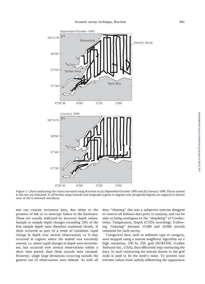

Page 3

sets canpresenceThese arSamplefirst samthese occhangeoccurreduneven,ent, butshort timHowevegeneral

Figure 1.in the texwest of th

941Acoustic survey technique, RoxAnn

by guest on July 22, 2011icesjm

s.oxfordjournals.orgD

ownloaded from

3°00'3°30'

58°00'

58°15'N

4°30' W 4°00'

57°45'

57°30'

3°00'3°30'

58°00'

(b)January 1996

58°15'N

4°30' W 4°00'

(a)September/October 1995

Helmsdale

Tarbet Ness

Spey Bay

Smith's Bank

57°45'

57°30'

Charts indicating the tracks surveyed using RoxAnn in (a) September/October 1995 and (b) January 1996. Places namedt are indicated. In all further maps latitude and longitude is given in degrees only (longitude degrees are negative to denotee Greenwich meridian).

contain erroneous data, due either to theof fish or to interrupt failure in the hardware.e usually indicated by incorrect depth values.to sample depth changes exceeding 10% of theple depth were therefore examined closely. Ifcurred as part of a trend of consistent rapidin depth over several observations, or if theyin regions where the seabed was extremely

i.e. where rapid changes in depth were inconsist-occurred over several observations within ae period, then these records were retained.

r, single large deviations occurring outside therun of observations were deleted. As with all

data ‘‘cleaning’’ this was a subjective exercise designedto remove all dubious data prior to analysis, and can beseen as being analogous to the ‘‘despiking’’ of Conduc-tivity, Temperature, Depth (CTD) recordings. Follow-ing ‘‘cleaning’’ between 13 000 and 14 000 recordsremained for each survey.Categorical data, such as sediment type or category,

were mapped using a nearest neighbour algorithm on ahigh resolution, 250 by 250, grid (SURFER, GoldenSoftware Inc., USA), thus effectively step contouring thedata. In such contouring the nearest datum to the gridnode is used to fix the node’s value. To prevent rareextreme values from unduly influencing the appearance

Page 4

E1

Sep

tem

ber/

Oct

ober

199

5E

2 S

epte

mbe

r/O

ctob

er 1

995

942 S. P. R. Greenstreet et al.

by guest on July 22, 2011icesjm

s.oxfordjournals.orgD

ownloaded from

–3.0

0

E1

Jan

uar

y 19

96

0–3

.50

–3.0

0

58.2

0

57.6

0 –4.5

0

58.0

0

57.8

0

–4.0

0–3

.50

E2

Jan

uar

y 19

96

–3.0

00

–3.5

0–3

.00

58.2

0

57.6

0 –4.5

0

58.0

0

57.8

0

–4.0

0–3

.50

1.8

1.7

1.6

1.5

1.4

1.3

1.2

1.1

1.0

0.9

0.8

0.7

0.6

0.5

0.4

0.3

0.2

0.1

1.8

1.7

1.6

1.5

1.4

1.3

1.2

1.1

1.0

0.9

0.8

0.7

0.6

0.5

0.4

0.3

2.0

1.9

ioninRoxAnn

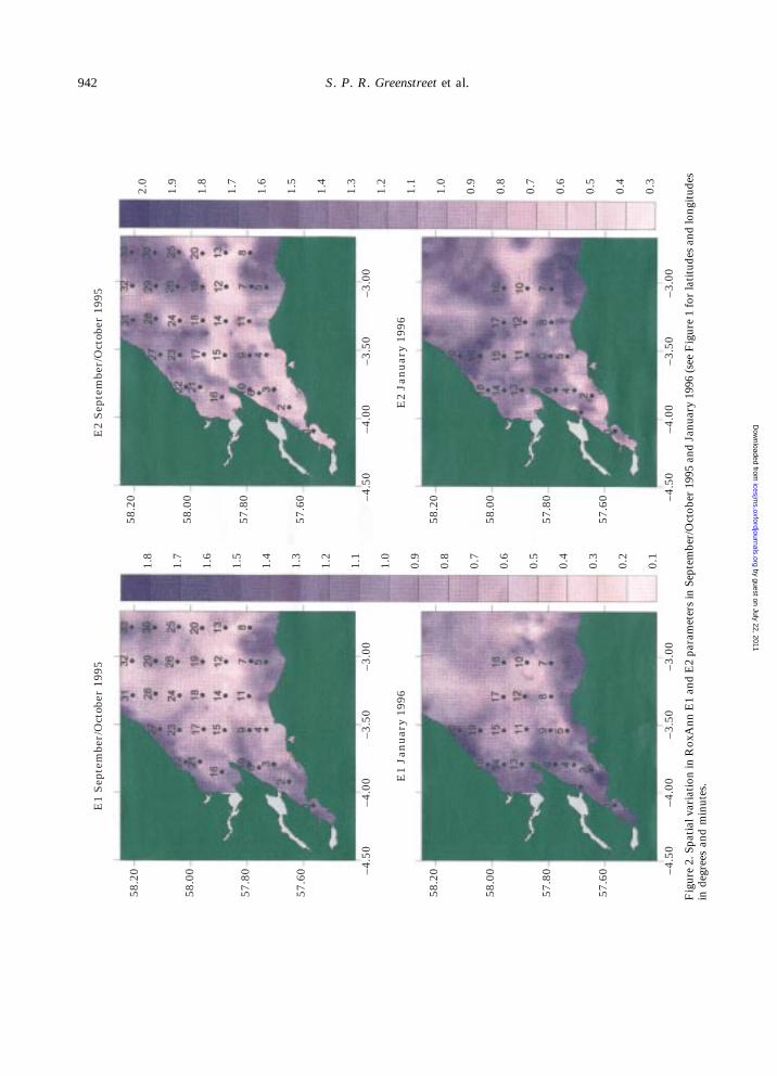
E1andE2parametersinSeptember/October1995andJanuary1996(seeFigure1forlatitudesandlongitudes

.

58.2

0

57.6

0 –4.5

0

58.0

0

57.8

0

–4.0

58.2

0

57.6

0 –4.5

0

58.0

0

57.8

0

–4.0

Figure2.Spatialvariat

indegreesandminutes

Page 5

of the mE1, and(usuallytrack disthe dataand 362data forContin

were ma1979; CdifficulticollectedOrd, 19

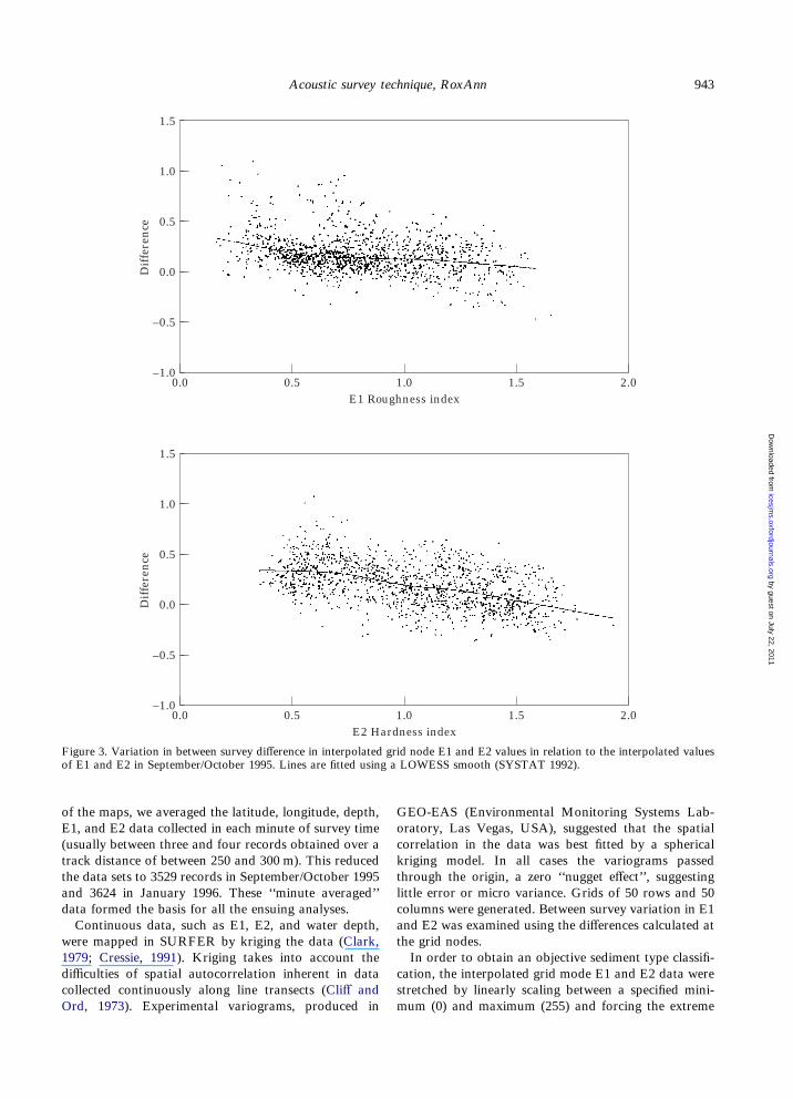
Figure 3.of E1 and

943Acoustic survey technique, RoxAnn

by guest on July 22, 2011icesjm

s.oxfordjournals.orgD

ownloaded from

2.0

1.5

–1.00.0

E2 Hardness index

Dif

fere

nce

1.0

0.5

0.0

–0.5

0.5 1.0 1.5

2.0

1.5

–1.00.0

E1 Roughness index

Dif

fere

nce

1.0

0.5

0.0

–0.5

0.5 1.0 1.5

Variation in between survey difference in interpolated grid node E1 and E2 values in relation to the interpolated valuesE2 in September/October 1995. Lines are fitted using a LOWESS smooth (SYSTAT 1992).

aps, we averaged the latitude, longitude, depth,E2 data collected in each minute of survey timebetween three and four records obtained over atance of between 250 and 300 m). This reducedsets to 3529 records in September/October 19954 in January 1996. These ‘‘minute averaged’’med the basis for all the ensuing analyses.uous data, such as E1, E2, and water depth,pped in SURFER by kriging the data (Clark,ressie, 1991). Kriging takes into account thees of spatial autocorrelation inherent in datacontinuously along line transects (Cliff and73). Experimental variograms, produced in

GEO-EAS (Environmental Monitoring Systems Lab-oratory, Las Vegas, USA), suggested that the spatialcorrelation in the data was best fitted by a sphericalkriging model. In all cases the variograms passedthrough the origin, a zero ‘‘nugget effect’’, suggestinglittle error or micro variance. Grids of 50 rows and 50columns were generated. Between survey variation in E1and E2 was examined using the differences calculated atthe grid nodes.In order to obtain an objective sediment type classifi-

cation, the interpolated grid mode E1 and E2 data werestretched by linearly scaling between a specified mini-mum (0) and maximum (255) and forcing the extreme

Page 6

Ari

thm

etic

dif

fere

nce

E1

Pro

port

ion

ate

diff

eren

ce E

1944 S. P. R. Greenstreet et al.

–3.0

0–4

.00

–3.5

0

Pro

port

ion

ate

diff

eren

ce E

2–3.0

0–4

.00

–3.5

0

4.00

2.00

1.00

0.50

0.25

0.00

–0.5

0

6.00

–0.2

5

1.50

1.00

0.50

0.25

0.00

–0.2

5

–1.0

0

2.00

–0.5

0

sexpressedasthearithm

eticdi

fferenceandasaproportion

of.

–3.0

0

58.2

0

57.6

0 –4.5

0

Ari

thm

etic

dif

fere

nce

E2

58.0

0

57.8

0

–4.0

0–3

.50

58.2

0

57.6

0 –4.5

0

58.0

0

57.8

0

–3.0

0

58.2

0

57.6

0 –4.5

0

58.0

0

57.8

0

–4.0

0–3

.50

58.2

0

57.6

0 –4.5

0

58.0

0

57.8

0

0.9

0.7

0.5

0.3

0.1

–0.1

–1.1

1.1

–0.3

–0.5

–0.7

–0.9

0.9

0.7

0.5

0.3

0.1

–0.1

–1.1

1.1

–0.3

–0.5

–0.7

–0.9

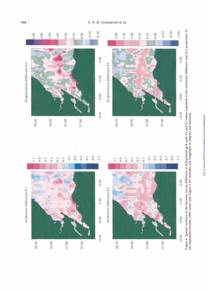
Figure4.Spatialvariationinthebetweensurveydi

fferenceininterpolatedgridnodeE1andE2value

theSeptember/October1995values(seeFigure1forlatitudesandlongitudesindegreesandminutes)

by guest on July 22, 2011icesjm

s.oxfordjournals.orgD

ownloaded from

Page 7

Sep

tem

ber/

Oct

ober

199

5S

epte

mbe

r/O

ctob

er 1

995

ab

945Acoustic survey technique, RoxAnn

2.25

dex1.50

1.75

2.00

6

2.25

dex1.50

1.75

2.00

gridnodedatawithobjective

.

2.25

2.25

E2

Har

dnes

s in

dex

E1 Roughness index

1.25

1.00

2.00

1.75

1.50

1.25

0.75

0.50

0.25

0.25

0.50

0.75

1.00

1.50

1.75

2.00

0.00

Jan

uar

y 19

962.

25

E2

Har

dnes

s in

E1 Roughness index

1.25

1.00

2.00

1.75

1.50

1.25

0.75

0.50

0.25

0.25

0.50

0.75

1.00

0.00

Jan

uar

y 19

9

2.25

2.25

E2

Har

dnes

s in

dex

E1 Roughness index

1.25

1.00

2.00

1.75

1.50

1.25

0.75

0.50

0.25

0.25

0.50

0.75

1.00

1.50

1.75

2.00

0.00

2.25

E2

Har

dnes

s in

E1 Roughness index

1.25

1.00

2.00

1.75

1.50

1.25

0.75

0.50

0.25

0.25

0.50

0.75

1.00

0.00

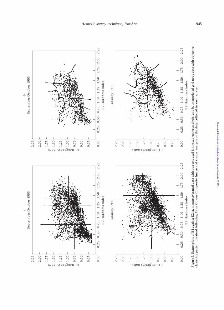
Figure5.ScatterplotsofE1againstE2:a,minuteaverageddatawithboxsetsusedinthesubjectiveanalysis;and

b,interpolated

clustering

patternobtainedfollowingFalseColourCom

positeImageandclusteranalysisofthedatacollectedineachsurvey

by guest on July 22, 2011icesjm

s.oxfordjournals.orgD

ownloaded from

Page 8

Su

bjec

tive

Obj

ecti

ve946 S. P. R. Greenstreet et al.

by guest on July 22, 2011icesjm

s.oxfordjournals.orgD

ownloaded from

–3.0

0

199

6

.50

–3.0

0

58.2

0

57.6

0 –4.5

0

58.0

0

57.8

0

–4.0

0–3

.50

Jan

uar

y 19

96

–3.0

0

tobe

r 19

95

.50

–3.0

0

58.2

0

57.6

0 –4.5

0

58.0

0

57.8

0

–4.0

0–3

.50

Sep

tem

ber/

Oct

ober

199

5

6 5 4 3 2 1

5 4 3 2 17 6 5 4 3 2 16

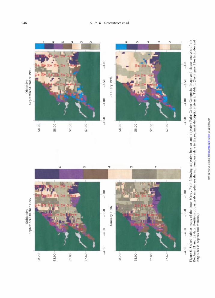
theinnerMoray

FirthfollowingsubjectiveboxsetandobjectiveFalseColourCom

positeImageandclusteranalysisofthe

sofdaygrab

samplesareshown,numbersrelatetothesedimentdescriptionsgiveninTable1.(SeeFigure1forlatitudesand

)

58.2

0

57.6

0 –4.5

0

Jan

uar

y

58.0

0

57.8

0

–4.0

0–3

58.2

0

57.6

0 –4.5

0

Sep

tem

ber/

Oc

58.0

0

57.8

0

–4.0

0–3

Figure6.Seabed

habitatmapsof

RoxAnn

E1andE2data.Position

longitudesindegreesandminutes.

Page 9

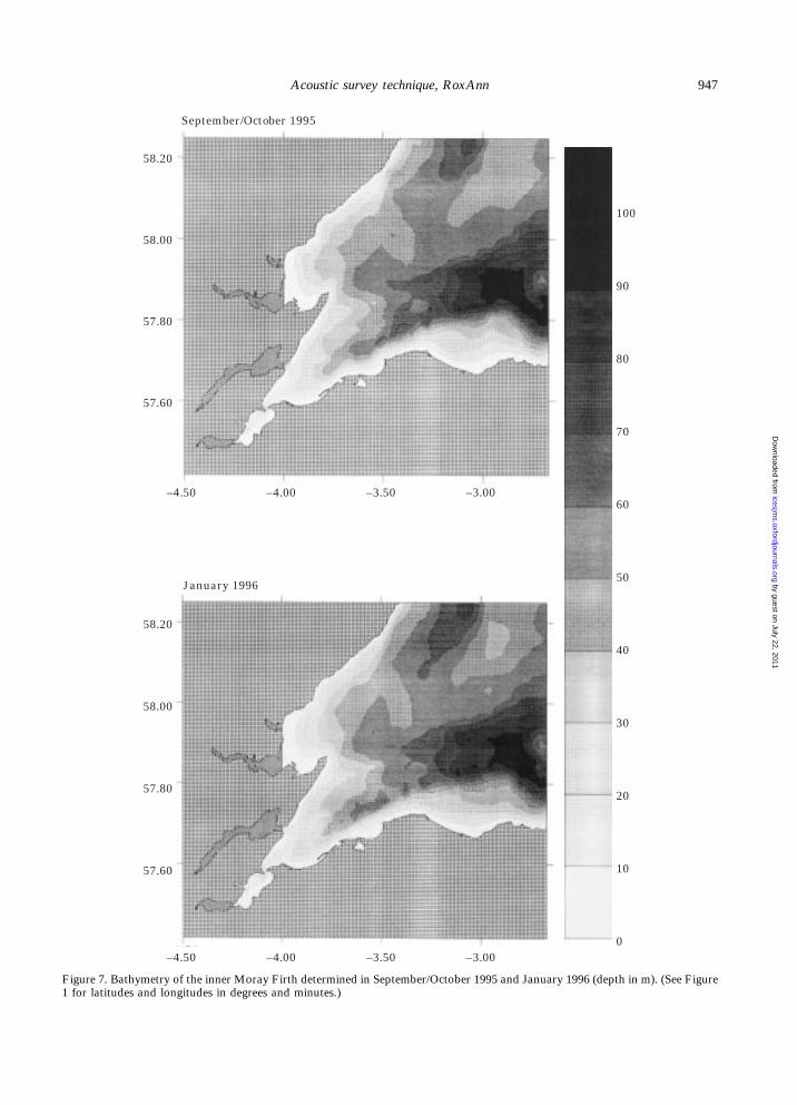
Figure 7.1 for latit

947Acoustic survey technique, RoxAnn

by guest on July 22, 2011icesjm

s.oxfordjournals.orgD

ownloaded from

58.20

57.60

January 1996

58.00

57.80

100

90

80

70

60

50

40

30

–3.00

58.20

57.60

–4.50

September/October 1995

58.00

57.80

–4.00 –3.50

20

10

–3.00–4.50 –4.00 –3.500

Bathymetry of the inner Moray Firth determined in September/October 1995 and January 1996 (depth in m). (See Figureudes and longitudes in degrees and minutes.)

Page 10

5% athe excreateametecolouspecifand rimagecationE1 ancarriegramsignifianalyThe cneareA

surve

948 S. P. R. Greenstreet et al.

by guest on July 22, 2011icesjm

s.oxfordjournals.orgD

ownloaded from

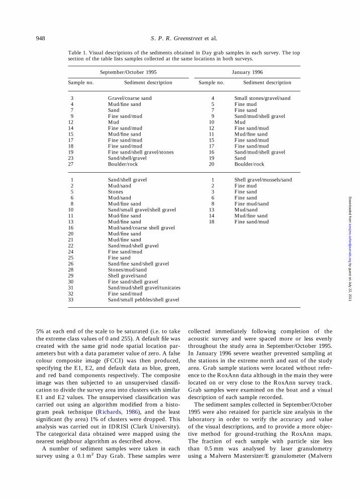
Table 1. Visual descriptions of the sediments obtained in Day grab samples in each survey. The topsection of the table lists samples collected at the same locations in both surveys.

September/October 1995 January 1996

Sample no. Sediment description Sample no. Sediment description

3 Gravel/coarse sand 4 Small stones/gravel/sand4 Mud/fine sand 5 Fine mud7 Sand 7 Fine sand9 Fine sand/mud 9 Sand/mud/shell gravel12 Mud 10 Mud14 Fine sand/mud 12 Fine sand/mud15 Mud/fine sand 11 Mud/fine sand17 Fine sand/mud 15 Fine sand/mud18 Fine sand/mud 17 Fine sand/mud19 Fine sand/shell gravel/stones 16 Sand/mud/shell gravel23 Sand/shell/gravel 19 Sand27 Boulder/rock 20 Boulder/rock

1 Sand/shell gravel 1 Shell gravel/mussels/sand2 Mud/sand 2 Fine mud5 Stones 3 Fine sand6 Mud/sand 6 Fine sand8 Mud/fine sand 8 Fine mud/sand10 Sand/small gravel/shell gravel 13 Mud/sand11 Mud/fine sand 14 Mud/fine sand13 Mud/fine sand 18 Fine sand/mud16 Mud/sand/coarse shell gravel20 Mud/fine sand21 Mud/fine sand22 Sand/mud/shell gravel24 Fine sand/mud25 Fine sand26 Sand/fine sand/shell gravel28 Stones/mud/sand29 Shell gravel/sand30 Fine sand/shell gravel31 Sand/mud/shell gravel/tunicates32 Fine sand/mud33 Sand/small pebbles/shell gravel

t each end of the scale to be saturated (i.e. to taketreme class values of 0 and 255). A default file wasd with the same grid node spatial location par-rs but with a data parameter value of zero. A falser composite image (FCCI) was then produced,ying the E1, E2, and default data as blue, green,ed band components respectively. The compositewas then subjected to an unsupervised classifi-to divide the survey area into clusters with similard E2 values. The unsupervised classification wasd out using an algorithm modified from a histo-peak technique (Richards, 1986), and the leastcant (by area) 1% of clusters were dropped. Thissis was carried out in IDRISI (Clark University).ategorical data obtained were mapped using thest neighbour algorithm as described above.number of sediment samples were taken in eachy using a 0.1 m2 Day Grab. These samples were

collected immediately following completion of theacoustic survey and were spaced more or less evenlythroughout the study area in September/October 1995.In January 1996 severe weather prevented sampling atthe stations in the extreme north and east of the studyarea. Grab sample stations were located without refer-ence to the RoxAnn data although in the main they werelocated on or very close to the RoxAnn survey track.Grab samples were examined on the boat and a visualdescription of each sample recorded.The sediment samples collected in September/October

1995 were also retained for particle size analysis in thelaboratory in order to verify the accuracy and valueof the visual descriptions, and to provide a more objec-tive method for ground-truthing the RoxAnn maps.The fraction of each sample with particle size lessthan 0.5 mm was analysed by laser granulometryusing a Malvern Mastersizer/E granulometer (Malvern

Page 11

Instrumewas anaused wit(4 mm)1/2Ö). Thof sampbution wtributionto "2ÖSimilarit26 partiBray–Cusional sc

949Acoustic survey technique, RoxAnn

by guest on July 22, 2011icesjm

s.oxfordjournals.orgD

ownloaded from

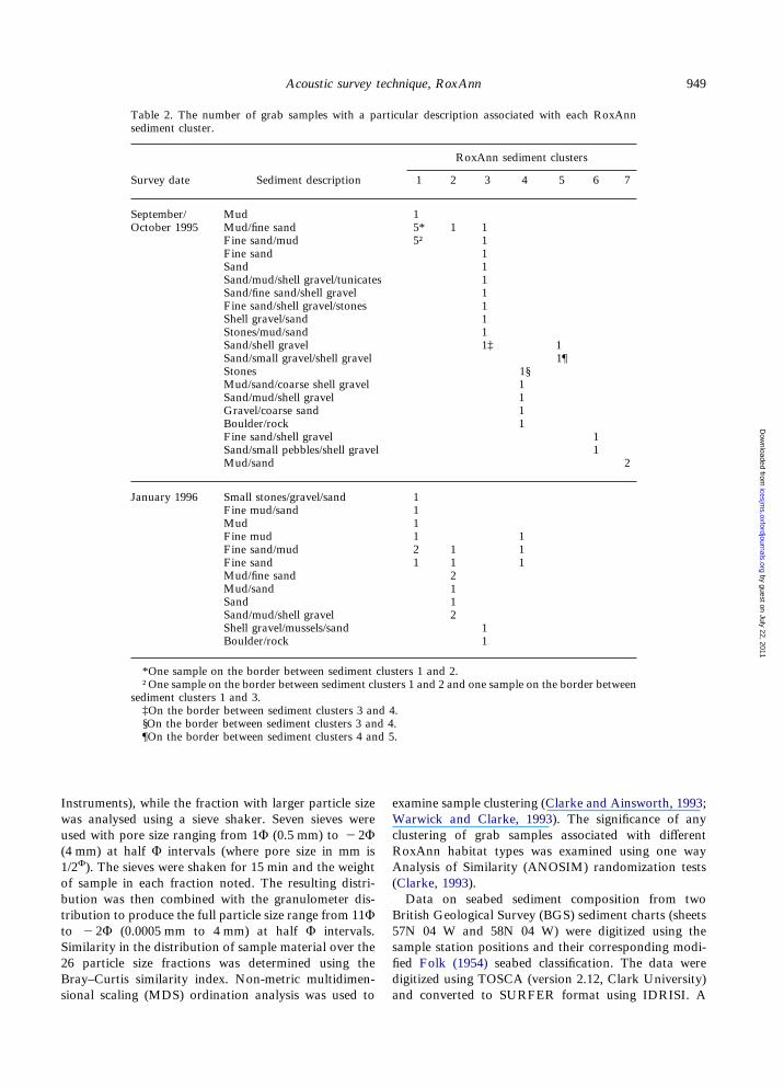
Table 2. The number of grab samples with a particular description associated with each RoxAnnsediment cluster.

Survey date Sediment description

RoxAnn sediment clusters

1 2 3 4 5 6 7

September/October 1995

MudMud/fine sand

15* 1 1

Fine sand/mud 5† 1Fine sand 1Sand 1Sand/mud/shell gravel/tunicates 1Sand/fine sand/shell gravel 1Fine sand/shell gravel/stones 1Shell gravel/sand 1Stones/mud/sand 1Sand/shell gravel 1‡ 1Sand/small gravel/shell gravel 1¶Stones 1§Mud/sand/coarse shell gravel 1Sand/mud/shell gravel 1Gravel/coarse sand 1Boulder/rock 1Fine sand/shell gravel 1Sand/small pebbles/shell gravel 1Mud/sand 2

January 1996 Small stones/gravel/sand 1Fine mud/sand 1Mud 1Fine mud 1 1Fine sand/mud 2 1 1Fine sand 1 1 1Mud/fine sand 2Mud/sand 1Sand 1Sand/mud/shell gravel 2Shell gravel/mussels/sand 1Boulder/rock 1

*One sample on the border between sediment clusters 1 and 2.†One sample on the border between sediment clusters 1 and 2 and one sample on the border between

sediment clusters 1 and 3.‡On the border between sediment clusters 3 and 4.§On the border between sediment clusters 3 and 4.¶On the border between sediment clusters 4 and 5.

nts), while the fraction with larger particle sizelysed using a sieve shaker. Seven sieves wereh pore size ranging from 1Ö (0.5 mm) to "2Öat half Ö intervals (where pore size in mm ise sieves were shaken for 15 min and the weightle in each fraction noted. The resulting distri-as then combined with the granulometer dis-to produce the full particle size range from 11Ö(0.0005 mm to 4 mm) at half Ö intervals.

y in the distribution of sample material over thecle size fractions was determined using thertis similarity index. Non-metric multidimen-aling (MDS) ordination analysis was used to

examine sample clustering (Clarke and Ainsworth, 1993;Warwick and Clarke, 1993). The significance of anyclustering of grab samples associated with differentRoxAnn habitat types was examined using one wayAnalysis of Similarity (ANOSIM) randomization tests(Clarke, 1993).Data on seabed sediment composition from two

British Geological Survey (BGS) sediment charts (sheets57N 04 W and 58N 04 W) were digitized using thesample station positions and their corresponding modi-fied Folk (1954) seabed classification. The data weredigitized using TOSCA (version 2.12, Clark University)and converted to SURFER format using IDRISI. A

Page 12

sedimproducolumthat oIm

1995,in thfittedlocatithe seInverpossiwas fiNorwheighobtaiSystesweptnumband pminedlengthpubli1989)valsspeciedensiwereexammostparamdistripropoCramKolm

Tablepartic

Surve

SeptemOctob

Janua

950 S. P. R. Greenstreet et al.

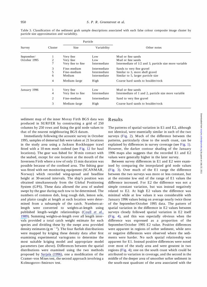
3. Classification of the sediment grab sample descriptions associated with each false colour composite image cluster byle size approximation and variability.

y Cluster

Particle

Other notesSize Variability

ber/er 1995

12

Very fineVery fine

LowLow

Mud or fine sandsMud or fine sands

7 Very fine to fine Intermediate Intermediate of 1/2 and 3, particle size more variable

3 Fine–medium Intermediate Sands to very fine gravel5 Fine–medium Intermediate Similar to 3, more shell gravel6 Medium Intermediate Similar to 5, larger particle size

4 Medium–large High Coarse hard sands to boulder/rock

ry 1996 1 Very fine Low Mud or fine sands4 Very fine to fine Intermediate Intermediate of 1 and 2, particle size more variable

2 Fine–medium Intermediate Sand to very fine gravel

3 Medium–large High Coarse hard sands to boulder/rock

m

e

nb

tnm

s.p

t

i

b

Dow

n

ent map of the inner Moray Firth BGS data wasced in SURFER by constructing a grid of 250ns by 250 rows and fixing the grid node values tof the nearest neighbouring BGS datum.ediately following the acoustic survey in Octobersamples of demersal fish were taken at 21 locationsstudy area using a Jackson Rockhopper trawlwith a 10 mm mesh codend (see Fig. 12 for haulons). The gear was fished for 30 min contact withabed, except for one location at the mouth of theess Firth where a tow of only 15 min duration wasle because of the confined area. The fishing geartted with net monitoring equipment (SCANMAR,ay) which recorded wing-spread and headlineat 30-second intervals. The ship’s position wased simultaneously from the Global Positioning(GPS). These data allowed the area of seabed

by the gear during each tow to be determined. Theers of common dab, long rough dab, lemon sole,laice caught at length at each location were deter-from a subsample of the catch. Numbers-at-were converted to weights-at-length using

hed length–weight relationships (Coull et al.,Summing weights-at-length over all length inter-rovided a total catch weight estimate for eachs and dividing these by the swept area providedy estimates (g m"2). The four flatfish distributionsmapped by kriging these density data after firstning experimental variograms to determine thesuitable kriging model and appropriate modeleters (see above). Differences between the spatialutions were examined using the two methodssed by Syrjala (1996), one a modification of theer–von Mises test, the second approach involving aogorov–Smirnov test.

Results

The patterns of spatial variation in E1 and E2, althoughnot identical, were essentially similar in each of the twosurveys (Fig. 2). Much of the difference between thepatterns, particularly close to the south coast, can beexplained by differences in survey coverage (see Fig. 1).However, the darker contour shading of the January1996 maps also suggests that the recorded E1 and E2values were generally higher in the later survey.Between survey differences in E1 and E2 were exam-

ined by comparing the interpolated grid node values(Fig. 3). Over much of the E1 range the differencebetween the two surveys was more or less constant, butat the extreme low end of the range of E1 values thedifference increased. For E2 the difference was not asimple constant variation, but was instead negativelyrelated to E2. At high E2 values the difference wasminimal while at low values it was considerable withJanuary 1996 values being on average nearly twice thoseof the September/October 1995 data. The pattern ofspatial variation in the difference in E2 values betweensurveys closely followed spatial variation in E2 itself(Fig. 4), and this was especially obvious when thedifference was expressed as a proportion of theSeptember/October 1995 E2 value. Positive differenceswere apparent in regions of softer sediment, while zeroor negative differences were observed where the sedi-ments were harder. No such spatial relationship wasapparent for E1. Instead positive differences were notedover most of the study area and were greatest in tworegions (Fig. 4); one on the south coast which could beattributed to variation in coverage, and the second in themiddle of the deeper area of smoother softer sediment inthe south-east quadrant of the area associated with the

by guest on July 22, 2011icesjm

s.oxfordjournals.orgloaded from

Page 13

presenceGreenstrPlots o

data indiagonal(Fig. 5avalues thmain baon thesemain baand thenseparatethe previ

Dim

ensi

on 2

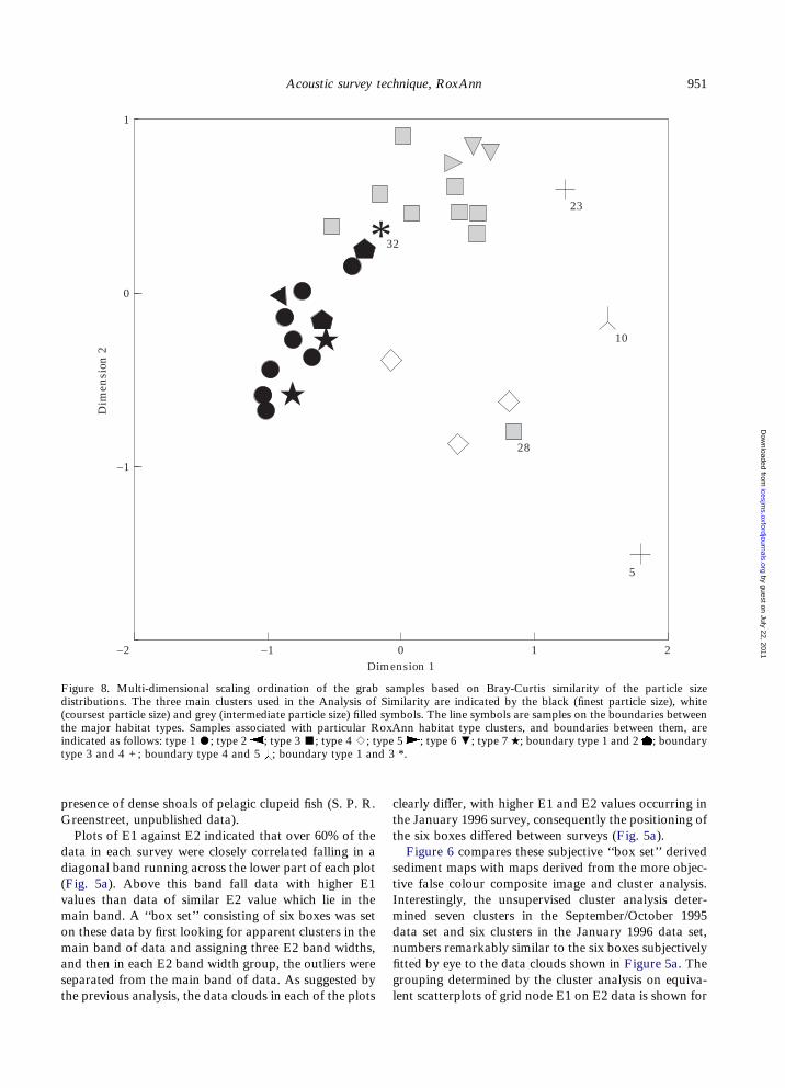
Figure 8distributi(coursestthe majorindicatedtype 3 an

951Acoustic survey technique, RoxAnn

by guest on July 22, 2011icesjm

s.oxfordjournals.orgD

ownloaded from

2

1

Dimension 11

0

–1

–1 0–2

*

★

★

32

23

10

28

5

. Multi-dimensional scaling ordination of the grab samples based on Bray-Curtis similarity of the particle sizeons. The three main clusters used in the Analysis of Similarity are indicated by the black (finest particle size), whiteparticle size) and grey (intermediate particle size) filled symbols. The line symbols are samples on the boundaries betweenhabitat types. Samples associated with particular RoxAnn habitat type clusters, and boundaries between them, areas follows: type 1 -; type 2 ; type 3 /; type 4 :; type 5 ; type 6 5; type 7 9; boundary type 1 and 2 ; boundaryd 4 +; boundary type 4 and 5 ; boundary type 1 and 3 *.

of dense shoals of pelagic clupeid fish (S. P. R.eet, unpublished data).f E1 against E2 indicated that over 60% of theeach survey were closely correlated falling in aband running across the lower part of each plot). Above this band fall data with higher E1an data of similar E2 value which lie in thend. A ‘‘box set’’ consisting of six boxes was setdata by first looking for apparent clusters in thend of data and assigning three E2 band widths,in each E2 band width group, the outliers wered from the main band of data. As suggested byous analysis, the data clouds in each of the plots

clearly differ, with higher E1 and E2 values occurring inthe January 1996 survey, consequently the positioning ofthe six boxes differed between surveys (Fig. 5a).Figure 6 compares these subjective ‘‘box set’’ derived

sediment maps with maps derived from the more objec-tive false colour composite image and cluster analysis.Interestingly, the unsupervised cluster analysis deter-mined seven clusters in the September/October 1995data set and six clusters in the January 1996 data set,numbers remarkably similar to the six boxes subjectivelyfitted by eye to the data clouds shown in Figure 5a. Thegrouping determined by the cluster analysis on equiva-lent scatterplots of grid node E1 on E2 data is shown for

Page 14

952 S. P. R. Greenstreet et al.

7.00

Rox

An

n c

lust

er3.

005

2.00

3.50

4.00

5.00

6.00

4.50

**

7.00 samplesassociatedwithdi

fferent

dary

betweenclusters1and2),

.

7.00

4 0

Rox

An

n c

lust

er

Sort coefficient

3.00

3 2 1

1.00

1.50

1.75

2.00

3.50

4.00

5.00

6.00

7.00

1.0

–0.5

Rox

An

n c

lust

er

Skewness

3.00

0.5

0.0

1.00

1.50

1.75

2.00

3.50

4.00

5.00

6.00

4 0

Kurtosis

3 2 1

1.00

1.50

1.7

4.50

4.50

*

*

7.00

8.00

000

0.03

125

Rox

An

n c

lust

er

Median diameter

3.00

1.00

1.50

1.75

2.00

3.50

4.00

5.00

6.00

4.50

80 –20

Rox

An

n c

lust

er

Percent silt

3.00

40 20 0

1.00

1.50

1.75

2.00

3.50

4.00

5.00

6.00

4.50

4.00

000

2.00

000

1.00

000

0.50

000

0.25

000

0.12

500

0.06

250

60

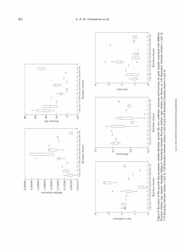
Figure9.Box

plotsoffiveparticlesizeparameters,mediandiameter,percentsilt,sortcoefficient,skewnessandkurtosis,forgrab

RoxAnn

habitattype

clusters.Samplesfalling

onboundariesbetweenRoxAnn

habitattype

clustersareshownas

1.50

(boun

1.75(boundarybetweenclusters1and3),3.50(boundarybetweenclusters3and4)and4.50(boundarybetweenclusters4and5)

by guest on July 22, 2011icesjm

s.oxfordjournals.orgD

ownloaded from

Page 15

comparitive metwhich armethodbetweenaries bevariable.Bathy

in the twdiscrepaand tidebetweenand sediments teshallowerougher.

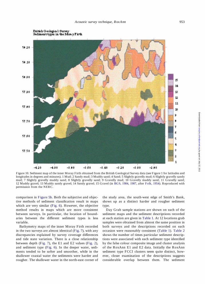
Figure 10longitudemud; 7 S12 Muddpermissio

953Acoustic survey technique, RoxAnn

by guest on July 22, 2011icesjm

s.oxfordjournals.orgD

ownloaded from

. Sediment map of the inner Moray Firth obtained from the British Geological Survey data (see Figure 1 for latitudes ands in degrees and minutes). 1 Mud; 2 Sandy mud; 3 Muddy sand; 4 Sand; 5 Slightly gravelly mud; 6 Slightly gravelly sandylightly gravelly muddy sand; 8 Slightly gravelly sand; 9 Gravelly mud; 10 Gravelly muddy sand; 11 Gravelly sand;y gravel; 13 Muddy sandy gravel; 14 Sandy gravel; 15 Gravel (in BGS, 1984, 1987, after Folk, 1954). Reproduced withn from the NERC.

son in Figure 5b. Both the subjective and objec-hods of sediment classification result in mapse very similar (Fig. 6). However, the objectiveresults in maps which are more consistentsurveys. In particular, the location of bound-tween the different sediment types is less

metry maps of the inner Moray Firth recordedo surveys are almost identical (Fig. 7), with anyncies explained by survey coverage differencesstate variation. There is a close relationshipdepth (Fig. 7), the E1 and E2 values (Fig. 2),ment type (Fig. 6). In the deeper water, sedi-nded to be softer and smoother, while in ther coastal water the sediments were harder andThe shallower water in the north-east corner of

the study area, the south-west edge of Smith’s Bank,shows up as a distinct harder and rougher sedimenttype.Day Grab sample stations are shown on each of the

sediment maps and the sediment descriptions recordedat each station are given in Table 1. At 12 locations grabsamples were obtained from almost the same position inboth surveys and the descriptions recorded on eachoccasion were reasonably consistent (Table 1). Table 2shows the number of times particular sediment descrip-tions were associated with each sediment type identifiedby the false colour composite image and cluster analysisof the RoxAnn E1 and E2 data. Initially the RoxAnnsediment type FCCI clusters seem quite distinct, how-ever, closer examination of the descriptions suggestsconsiderable overlap between them. The sediment

Page 16

descrficatioand o(Tablsandsstrateof subouldRoxAfor eaMD

CurtiRoxAANOwas hexcluwithsedimdue tmentcompof p<compwithandcluste5, an(as sclusteonlypairw

1

Dep

th (

m)

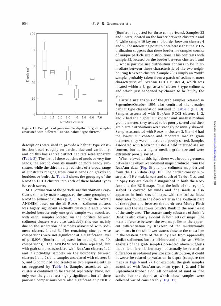
Figureassoci

954 S. P. R. Greenstreet et al.

Dow

nloaded fro

(Bonferoni adjusted for three comparisons). Samples 23and 5 were located on the border between clusters 3 and4, while sample 10 lay on the border between clusters 4and 5. The interesting point to note here is that the MDSordination suggests that these borderline samples consistof unique particle size distributions. This contrasts withsample 32, located on the border between clusters 1 and3, whose particle size distribution appears to be inter-mediate between those characteristic of the two neigh-bouring RoxAnn clusters. Sample 28 is simply an ‘‘odd’’sample, probably taken from a patch of sediment morecharacteristic of RoxAnn FCCI cluster 4, which waslocated within a larger area of cluster 3 type sediment,and which just happened by chance to be hit by thegrab.Particle size analysis of the grab samples retained in

September/October 1995 also confirmed the broaderhabitat type classification outlined in Table 3 (Fig. 9).Samples associated with RoxAnn FCCI clusters 1, 2,and 7 had the highest silt content and smallest mediangrain diameter, they tended to be poorly sorted and theirgrain size distributions were strongly positively skewed.Samples associated with RoxAnn clusters 3, 5, and 6 had

7.05.01.0 2.0 3.0 4.01.5 6.0

00

0

RoxAnn cluster

80

60

40

20

11. Box plots of grab sample depths for grab samplesated with different RoxAnn habitat type clusters.

iptions were used to provide a habitat type classi-n based roughly on particle size and variability,n this basis three distinct habitats were apparente 3). The first of these consists of muds or very fine, the second consists mainly of more sandy sub-s, while the third habitat consists of a broad rangebstrates ranging from coarse sands or gravels toers or bedrock. Table 3 shows the grouping of thenn FCCI clusters into each of these habitat typesch survey.S ordination of the particle size distribution Bray–s similarity matrix suggested the same grouping ofnn sediment clusters (Fig. 8. Although the overallSIM based on the all RoxAnn sediment clustersighly significant (actually clusters 2 and 5 wereded because only one grab sample was associatedeach; samples located on the borders betweenent clusters were also excluded), this was mainlyo the separation of samples associated with sedi-clusters 1 and 3. The remaining nine pairwisearisons were not significant at a significance level0.005 (Bonferoni adjusted for multiple, i.e. 10,arisons). The ANOSIM was then repeated, butgrab samples associated with RoxAnn clusters 1, 2,7 (including samples on the boundary betweenrs 1 and 2), and samples associated with clusters 3,d 6 combined and treated as two separate entitiesuggested by Table 3). Samples associated withr 4 continued to be treated separately. Now, notwas the global test highly significant, but all threeise comparisons were also significant at p<0.017

the lowest silt content and moderate median graindiameter; they were moderate to poorly sorted. Samplesassociated with RoxAnn cluster 4 held intermediate siltcontent, but had a higher median grain size and wereextremely poorly sorted.When viewed in this light there was broad agreement

between the objective sediment maps produced from theRoxAnn data (Fig. 6) and the sediment map derivedfrom the BGS data (Fig. 10). The harder coarser sub-strates off Helmsdale, east and south of Tarbet Ness andin Spey Bay are clearly distinguished in both the Rox-Ann and the BGS maps. That the bulk of the region’sseabed is covered by muds and fine sands is alsoapparent in both sets of maps, with the softest finestsubstrates found in the deep water in the southern partof the region and between the north-west Moray Firthcoast and the shallower Smith’s Bank in the north-eastof the study area. The coarser sandy substrate of Smith’sBank is also clearly evident in both sets of maps. Themain difference between the two maps lies in the appar-ent differentiation by RoxAnn of the muddy/sandysediments in the shallower waters close to the coast linein the western parts of the study area from apparentlysimilar sediments further offshore and to the east. Whileanalysis of the grab samples presented above suggeststhat this differentiation may not actually be related todifferences in sediment particle size distribution, it couldhowever be related to variation in depth (compare themaps in Figs 6 and 7). For example, the grab samplesassociated with RoxAnn sediment types 1, 2, and 7 inSeptember/October 1995 all consisted of mud or finesands, but the depth at which these samples werecollected varied considerably (Fig. 11).

by guest on July 22, 2011icesjm

s.oxfordjournals.orgm

Page 17

100

80

Km

Eas

t

Km North

60 40 20

2040

6080

0

0.00

0.05

0.10

0.15

0.20

0.25

0.30

0.35

0.40

100

80

Km

Eas

t

Km North

60 40 20

2040

6080

0

0.00

0.05

0.10

0.15

0.20

0.25

0.30

0.35

0.40

0.45

0.50

0.55

0.60

0.65

Lem

on S

ole

Pla

ice

100

80

Km

Eas

t

Km North60 40 20

2040

6080

0

0.00

0.60

0.10

0.50

0.20

0.70

0.30

0.80

0.40

100

80

Km

Eas

t

Km North

60 40 20

2040

6080

0

0.00

0.05

0.10

0.15

0.20

0.25

0.30

0.35

0.40

0.45

Lon

g R

ough

Dab

Com

mon

Dab

0.90

1.10

1.20

1.30

1.40

1.50

1.60

1.70

1.00

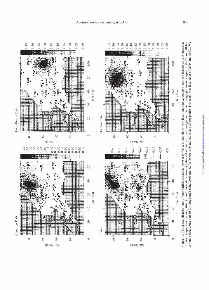
Figure12.ThespatialdistributionsoffourflatfishspeciesintheMorayFirth.Pointsshow

trawllocationsandvaluesgiverecordeddensityateachlocation.

Contourmapswerederivedafterkrigingthesedatausingasphericalmodelwithzeronuggetandsillandrangeparametersequalto0.270and40

for

common

dab,0.013and30forlong

roughdab,0.036and32forlemon

soleand0.018and35forplaice.Theoriginwaslocatedat57

)25*Nand004)30

*W.

955Acoustic survey technique, RoxAnn

by guest on July 22, 2011icesjm

s.oxfordjournals.orgD

ownloaded from

Page 18

Figdab,1995.sole,ever,signifiFurthcommsignifiand tpointall sigMostFine3). Osedimthe tsedimsuggebe fopossiflatfisdepth0–35shallomentsedimspeciesedimmoststratamentmostPlaicewatersometransvaluerange

Tableencesrough1995.fied Cthe K

CommLongLemoPlaice

Sign

956 S. P. R. Greenstreet et al.

samples sizes involved are largely responsible for ourfailure to produce statistically significant results in thisinstance. Given our small sample sizes, the relativelysmall probabilities may well be indicative that the sedi-ment habitats detected by RoxAnn influence the spatialdistributions of the four flatfish species.

Discussion

The present paper highlights some important aspects inthe analysis and application of RoxAnn data for habitatdiscrimination. There were systematic differences in theE1 and E2 values recorded at the same locationsbetween the two surveys. Although it is impossible to be

4. Results of Syrjala’s (1996) tests for significant differ-between the spatial distributions of common dab, longdab, lemon sole and plaice in the Moray Firth in OctoberLower left section gives results obtained from the modi-ramer-von Mises test, upper right section shows results ofolmogorov-Smirnov approach.

Commondab

Longrough dab

Lemonsole Plaice

on dab – 0.007** 0.405 0.007**rough dab 0.225 – 0.002** 0.406n sole 0.372 0.046* – 0.007**

0.006** 0.637 0.007** –

ificance levels indicated by *(p<0.05) and ** (p<0.01).

by guest on July 22, 2011icesjm

s.oxfordjournals.orgD

ownloaded from

ure 12 shows the spatial distributions of commonlong rough dab, lemon sole, and plaice in OctoberWith the exception of common dab and lemonthese distributions appear quite dissimilar. How-formal testing indicated that there was also nocant difference between plaice and long rough dab.ermore, the difference between the distributions ofon dab and long rough dab was only statisticallycant when using the Kolmogorov–Smirnov testhis test can be unduly influenced by large singledeviations. The three remaining comparisons werenificant no matter which test was used (Table 4).of the demersal hauls occurred in areas of Veryto Fine or Fine to Medium particle size (see Tablenly two hauls were located in the third, coarser,ent habitat type; we therefore combined these withrawl samples taken from the Fine to Mediument habitat. Comparison between Figures 12 and 7sts that the highest densities of each species were tound in areas of deeper water. In examining the

certain why this should be, a number of suggestions canbe made. The most likely cause of differences is variationin the attitude of the transducer. The theoretical basis ofRoxAnn (Chivers et al., 1990) assumes that the trans-ducer is generally horizontal. The values of both E1 andE2 are likely to be affected when this assumption isviolated. The towed body used in this survey (and inmost similar situations) is actively hydrodynamic. Evenslight accidental damage of the fins (e.g. bending) willcause the towed body to take up a subtly differentattitude. However, for this type of survey the towedbody is generally preferable to the hull mounted optiondespite these potential drawbacks. Provided the towedbody is protected from damage during a survey, it isreasonable to assume that its attitude will remain rela-tively constant. In addition, variation in the towedbody’s attitude can be monitored with heel and pitchsensors and corrective action taken in the event of asignificant change. The greatest advantage of towedbodies is that their performance is relatively independentof the weather. It is almost impossible to ensure that thetrim of a vessel does not change constantly during a

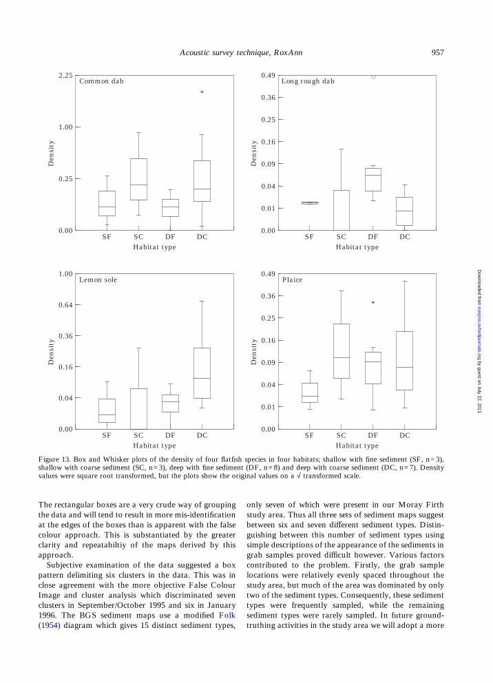
ble effect of the two sediment habitat types onh density therefore, we also took variation in waterinto account by considering two depth strata,

m and >35 m. This gave a total of four habitats,w with fine sediment, shallow with coarse sedi-, deep with fine sediment, and deep with coarseent. The Box and Whisker plots suggest that eachs responded differently to various combinations ofent habitat and depth (Fig. 13). Common dab wereabundant in coarser sediments at both depth. Long rough dab appeared to prefer fine sedi-s in deeper water, while lemon sole tended to beabundant in coarse sediments in deeper water.appeared to avoid fine sediment habitat in shallow. These patterns should however be treated withcaution since analyses of variance (on the root-formed data) were not statistically significant (ps for the sediment habitat variable for exampled from 0.09 to 0.21). We believe that the small

survey, not only due to wave action, but also throughfuel and water use. Systematic differences could alsoarise as a result of seasonal changes. At 38 kHz soundcan penetrate a considerable distance into the seabed,perhaps up to 1 m depending on sediment density andwater content. It is likely therefore that the infaunal aswell as epifaunal benthic biota may affect the values ofE1 and E2 (e.g. Magorrian et al., 1995). There are likelyto be seasonal changes in the abundance and distri-bution of such organisms, which may modulate theRoxAnn parameters.These observations highlight the requirement to

ground truth any RoxAnn survey data on the samesurvey, and to conduct the analysis on the basis of thesesamples. The false colour and clustering techniquedescribed here is particularly useful in this context, as itdoes not work on the basis of a fixed relationshipbetween E1, E2 and a specific substrate. This techniquealso avoids the problem associated with the ‘‘box set’’.

Page 19

The rectthe dataat the edcolour aclarity aapproacSubjec

patternclose agImage aclusters1996. T(1954) d

1.0

0.0

Den

sity

0.6

0.3

0.1

0.0

2.2

0.0

Den

sity

1.0

0.2

Figure 13shallow wvalues we

957Acoustic survey technique, RoxAnn

by guest on July 22, 2011icesjm

s.oxfordjournals.orgD

ownloaded from

0

0

Habitat type

4

6

6

4

SF SC DF DC

Lemon sole0.49

0.00

Habitat type

Den

sity

0.25

0.16

0.09

0.04

SF SC DF DC

Plaice

5

0

Habitat type

0

5

SF SC DF DC

Common dab0.49

0.00

Habitat typeD

ensi

ty

0.25

0.16

0.09

0.04

SF SC DF DC

Long rough dab

0.36

0.01

*

*0.36

0.01

. Box and Whisker plots of the density of four flatfish species in four habitats; shallow with fine sediment (SF, n=3),ith coarse sediment (SC, n=3), deep with fine sediment (DF, n=8) and deep with coarse sediment (DC, n=7). Densityre square root transformed, but the plots show the original values on a √ transformed scale.

angular boxes are a very crude way of groupingand will tend to result in more mis-identificationges of the boxes than is apparent with the falsepproach. This is substantiated by the greaternd repeatabiltiy of the maps derived by thish.tive examination of the data suggested a boxdelimiting six clusters in the data. This was inreement with the more objective False Colournd cluster analysis which discriminated sevenin September/October 1995 and six in Januaryhe BGS sediment maps use a modified Folkiagram which gives 15 distinct sediment types,

only seven of which were present in our Moray Firthstudy area. Thus all three sets of sediment maps suggestbetween six and seven different sediment types. Distin-guishing between this number of sediment types usingsimple descriptions of the appearance of the sediments ingrab samples proved difficult however. Various factorscontributed to the problem. Firstly, the grab samplelocations were relatively evenly spaced throughout thestudy area, but much of the area was dominated by onlytwo of the sediment types. Consequently, these sedimenttypes were frequently sampled, while the remainingsediment types were rarely sampled. In future ground-truthing activities in the study area we will adopt a more

Page 20

stratified sampling regime to ensure equal sampling ofthe less common sediment types. Secondly, actuallydescribing in words the appearance of a grab sample wasnot simple, consequently most samples acquired aunique description and relating these numerous variousdescriptions to the six or seven RoxAnn FCCI clusterswas not easy. Refinement of the grab sample visualappearance descriptions, and MDS ordination analysisof particle size distributions, suggested that, on the basisof the data available to date, we could only resolve threesediment habitats with certainty in the inner MorayFirth using RoxAnn.Analyses of both RoxAnn surveys indicated substrate

differences in inshore areas which were not apparent ineither the grab samples or the BGS data. However,RoxAnn is not only sensitive to physical abiotic charac-teristics of the sediments; E1 and E2 can also beinfluenced by biotic features associated with the seabedsuch as the abundance of particular benthic organisms(Magorrian et al., 1995). The apparently different habi-tats defined by RoxAnn in the inner Moray Firth wererestricted to shallower water of generally less than 30 mdepth. It is entirely possible that some biotic feature,such as the presence of seaweed, may have been respon-sible for this habitat distinction, rather than anyvariation in sediment type (e.g. Schlagintweit, 1993).Alternatively, water depth, or perhaps closer proximityto freshwater outflows, might affect the performance ofRoxAnn or influence characteristics of the seabed, suchas sediment compaction, water content and large-scale‘‘roughness’’, e.g. sand ripples, to which RoxAnn issensitive, but which do not show up in simple visualexamination of the grab samples or in particle sizeanalysis. One final possible explanation is that the toplayer of soft mud/sand substrates sampled by the grab isless thick in the shallower water exposed to strongertides, and that RoxAnn is responding to denser hardersubstrate layers below the surface of the seabed. Ingener(RoxusedsurvesubtidTo

distinrepeaanalyniqueexamsedimsensitby Rdifferpossienceschara

sampidentihabitmeantats ofinerabseninshosurveof Roclustebe hsedimthe sebiolofish stherresultNorthwouldbrateSuchgenerabundTh

of maof eff6, inlaborerablylar mBGSdata cactiviClupeand vmamm

k

thirGist. Ocnuvesea

958 S. P. R. Greenstreet

by guest on July 22, 2011icesjm

s.oxfordjournals.orgD

ownloaded from

al, it is recommended by Marine MicrosystemsAnn’s manufacturers) that different box settings bein water shallower than 30 m. The results of thisy emphasize the importance of treating shallowal areas differently to more offshore areas.conclude, RoxAnn provided an efficient means ofguishing differences in seabed habitat that weretable, particularly when the E1 and E2 data weresed using False Colour Image and clustering tech-s. However, when compared with simple visualination and particle size distribution analysis ofent grab samples, RoxAnn appeared over-

Ac

WetheM.assseaformaSurRe

ive. Some of the different sediment types resolvedoxAnn could not be characterized in terms ofence in sediment grain size. It remains entirelyble however, that RoxAnn is identifying real differ-in habitat and that it is responding to othercteristics of the seabed that sediment grab

RefeBGS.Brit

BGS.Brit

ling cannot detect. Even if we can, at this point,fy with certainty only three different sedimentats in the inner Moray Firth, this in itself is noachievement when one considers that these habi-nly range from muddy sands to fine gravels. Themuds and the coarser, harder sediments are almostt from our study area, or are restricted to closere regions which were not easily covered by they vessel. Our results suggest, therefore, that the usexAnn, combined with False Colour Image andr analysis, to map seabed habitat variation wouldighly effective in areas containing more variedent habitats. The flatfish density data suggest thatdiment habitats discerned by RoxAnn may holdgical significance in influencing the distribution ofpecies strongly associated with the seabed. If fur-work confirms the statistical significance of this, then RoxAnn surveys of regions such as theSea may provide valuable information whichallow surveys of groundfish and benthic inverte-species to be designed on a stratified random basis.designs, where they can be realistically applied,ally provide more precise estimates of speciesance (Simmonds and Fryer, 1996).e final point to make concerns the cost-effectivenesspping sea bed habitat in this manner. The amountort required to produce the maps shown in Figureterms of shipboard sea-time and time in theatory necessary for grab sample analysis, is consid-less than the resources required to produce simi-aps using more traditional methods, such as thegrab survey (Fig. 10). Furthermore, the RoxAnnan be collected while the vessel is occupied in otherties. In this instance, RoxAnn was deployed whilea was engaged in acoustic surveys of pelagic fishisual count transect surveys of seabirds and marineals.

nowledgements

ank the officers and crew of RFV Clupea for allpatience and assistance during the two cruises, I.ibb, J. A. McMillan, M. A. Bell, and M. Hardinged with data acquisition and sample collection atur thanks are due to Steve Hall and John Hisloponstructive comments on an earlier draft of thescript. Permission to use the British Geologicaly data was granted by the Natural Environmentalrch Council.

et al.

rences1984. Moray–Buchan sea bed sediments and quaternary.ish Geological Survey, 57 N 04 W.1987. Caithness sea bed sediments and quaternary.ish Geological Survey, 58 N 04 W.

Page 21

Basford, D. and Eleftheriou, A. 1988. The benthic environmentof the North Sea (56) to 61)N). Journal of the MarineBiological Association of the UK, 68: 125–141.

Carbone, C. and Houston, A. I. 1994. Patterns in the divingbehaviour of the pochard, Aythya ferina: a test of anoptimality model. Animal Behaviour, 48: 457–465.

Catchpole, C. K. 1974. Habitat selection and breeding successin the reed warbler (Acrocephalus scirpaceus). Journal ofAnimal Ecology, 43: 363–380.

Chivers, R. C., Emerson, N. C., and Burns, D. 1990. Newacoustic processing for underway surveying. The Hydro-graphic Journal, 56: 9–17.

Clark, I. 1979. Practical geostatistics. Elsevier, London.Clarke, K. R. 1993. Non-parametric multivariate analysesof changes in community structure. Australian Journal ofEcology, 18: 117–143.

Clarke, K. R. and Ainsworth, M. 1993. A method of linkingmultivariate community structure to environmental vari-ables. Marine Ecology Progress Series, 92: 205–219.

Cliff, A. D. and Ord, J. K. 1973. Spatial autocorrelation. Pion,London.

Coull, K. A., Jermyn, A. S., Newton, A. W., Henderson, G. I.,and Hall, W. B. 1989. Length/weight relationships for 88species of fish encountered in the North East Atlantic.Scottish Fisheries Research Report, 43: 81pp.

Cressie, N. A. C. 1991. Statistics for spatial data. Wiley, NewYork.

Douglass, R. J. 1976. Spatial interactions and microhabitatselections of two locally sympatric voles, Microtus montanusand Microtus pennsylvanicus. Ecology, 57: 346–352.

Duineveld, G. C. A., Kunitzer, A., Niermann, U., De Wild,P. A. W. J., and Gray, J. S. 1991. The macro-benthos of theNorth Sea. Netherlands Journal of Sea Research, 28: 53–65.

Eadie, J. McA. and Keast, A. 1984. Resource heterogeneity andfish species diversity in lakes. Canadian Journal of Zoology,62: 1689–1695.

Folk, R. L. 1954. The distinction between grain size andmineral composition in sedimentary-rock nomenclature.Journal of Geology, 62: 344–359.

Fretwell, S. D. and Lucas, H. L. 1970. On territorial behaviourand other factors influencing habitat distribution in birds.Acta Biotheoretica, 19: 16–36.

Greenstreet, S. P. R. 1996. Estimation of the daily consumptionof food by fish in the North Sea in each quarter of the year.Scottish Fisheries Research Report, 55: 16pp plus tables.

Heip, C., Basford, D., Craeymeersch, J. A., Dewarumez, J.-M.,Dorjes, J., de Wilde, P., Duineveld, G., Eleftheriou, A.,Herman, P. M. J., Niermann, U., Kingston, P., Kunitzer, A.,Rachor, E., Rumohr, H., Soetaert, K., and Soltwedel, T.1992. Trends in biomass, density and diversity of North Seamacrofauna. ICES Journal of Marine Science, 49: 13–22.

Hiscock, K. 1990. Marine Nature Conservation Revue:Methods. N.C.C., C.S.D. report No. 1072.

Holbrook, S. J. and Schmitt, R. J. 1988. The combined effectsof predation risk and food reward on patch selection. Ecol-ogy, 69: 125–134.

Huston, A. H. 1994. Biological Diversity: The coexistence ofspecies on changing landscapes. Cambridge University Press,681pp.

Kaiser, M. J. and Spencer, B. E. 1996. The effects of beam-trawl disturbance on infaunal communities in differenthabitats. Journal of Animal Ecology, 65: 348–358.

King, C. E. and Dawson, P. S. 1973. Habitat selection by flourbeetles in complex environments. Physiological Zoology, 46:297–309.

MacArthur, R. H. and MacArthur, J. W. 1961. On bird speciesdiversity. Ecology, 42: 594–598.

Magorrian, B. H., Service, M., and Clarke, W. 1995. Anacoustic bottom classification survey of Strangford Lough,Northern Ireland. Journal of the Marine Biological Associ-ation of the UK, 75: 987–992.

Milinski, M. and Parker, G. A. 1991. Competition forresources. In Behavioural ecology: an evolutionary approach.Third edition. pp. 137–168. Ed. by J. R. Krebs and N. B.Davies. Blackwell Scientific Publications, Oxford, England.

Partridge, L. 1978. Habitat selection. In Behavioural ecology:An evolutionary approach first edition. pp. 351–376. Ed. byJ. R. Krebs and N. B. Davies. Blackwell Scientific Publi-cations, Oxford, England.

Perry, R. I. and Smith, S. J. 1994. Identifying habitat associ-ations of marine fishes using survey data: an application tothe northwest Atlantic. Canadian Journal of Fisheries andAquatic Sciences, 51: 589–602.

Rand, A. S. 1964. Ecological distribution in anoline lizards ofPuerto Rico. Ecology, 45: 745–752.

Richards, J. A. 1986. Remote sensing digital image analysis: Anintroduction. Springer, Berlin.

Rosenzweig, M. L. 1995. Species diversity in time and space.Cambridge University Press, UK. 436pp.

Schlagintweit, G. E. O. 1993. Real-time Acoustic BottomClassification for Hydrography: a Field Evaluation ofRoxAnn. Canadian Hydrographic Services, Departmentof Fisheries and Oceans, Canada. 16pp.

Schwinghamer, P., Guigne, J. Y., and Siu, W. C. 1996. Quan-tifying the impact of trawling on benthic habitat structureusing high resolution acoustics and chaos theory. CanadianJournal of Fisheries and Aquatic Sciences, 53: 288–296.

Simmonds, E. J. and Fryer, R. J. 1996. Which are better,random or systematic acoustic surveys? A simulation usingNorth Sea herring as an example. ICES Journal of MarineScience, 53: 39–50.

Smith, S. J. and Page, F. H. 1996. Associations betweenAtlantic cod (Gadus morhua) and hydrographic variables:implications for the management of the 4VsW cod stock.ICES Journal of Marine Science, 53: 597–614.

Syrjala, S. E. 1996. A statistical test for a difference between thespatial distribution of two populations. Ecology, 77: 75–80.

SYSTAT 1992. SYSTAT for Windows, Version 5 edition.Systat Inc., Evanston, IL, USA. pp. 636.

Thompson, P. M., Pierce, G. J., Hislop, J. R. G., Miller, D.,and Diack, J. S. W. 1991. Winter foraging by common seals(Phoca vitulina) in relation to food availability in the innerMoray Firth, N.E. Scotland. Journal of Animal Ecology, 60:283–294.

Thompson, P. M., Tollit, D. J., Greenstreet, S. P. R., Mackay,A., and Corpe, H. M. 1996. Between year variations in thediet and behaviour of harbour seals (Phoca vitulina) in theMoray Firth; causes and consequences. In Aquatic predatorsand their prey. Ed. by S. P. R. Greenstreet and M. L. Tasker.Blackwells’ Science Ltd, Oxford, England.

Turner, A. M. 1996. Freshwater snails alter habitat use inresponse to predation. Animal Behaviour, 51: 747–756.

Warwick, R. M. and Clarke, K. R. 1993. Comparing theseverity of disturbance: a meta-analysis of marine macroben-thic data. Marine Ecology Progress Series, 92: 221–231.

Wecker, S. C. 1963. The role of early experience in habitatselection by the prairie deermouse Peromyscus maniculatusbairdi. Ecological Monographs, 33: 307–325.

Werner, E. E. 1977. Species packing and niche complementarityin three sunfishes. American Naturalist, 111: 553–578.

959Acoustic survey technique, RoxAnn

by guest on July 22, 2011icesjm

s.oxfordjournals.orgD

ownloaded from