An assessment of future extreme precipitation in western ...

Hydrol. Earth Syst. Sci., 14, 2329–2341, 2010www.hydrol-earth-syst-sci.net/14/2329/2010/doi:10.5194/hess-14-2329-2010© Author(s) 2010. CC Attribution 3.0 License.

Hydrology andEarth System

Sciences

An assessment of future extreme precipitation in western Norwayusing a linear model

G. N. Caroletti1,2 and I. Barstad1,3

1Bjerknes Centre for Climate Research, Bergen, Allegata 55, 5007 Bergen, Norway2Geophysical Institute, University of Bergen, Allegata 70, 5007 Bergen, Norway3Uni Research AS, Thormhlensgt. 55, 5008 Bergen, Norway

Received: 24 November 2009 – Published in Hydrol. Earth Syst. Sci. Discuss.: 18 December 2009Revised: 29 October 2010 – Accepted: 9 November 2010 – Published: 26 November 2010

Abstract. A Linear Model (Smith and Barstad, 2004)was used to dynamically downscale Orographic Precipita-tion over western Norway from twelve General CirculationModel simulations. The GCM simulations come from theA1B emissions scenario in IPCC’s 2007 AR4 report. Anassessment of the changes to future Orographic Precipita-tion (time periods: 2046–2065 and 2081–2100) versus thehistorical control period (1971–2000) was performed. Re-sults showed increases in the number of Orographic Precip-itation days and in Orographic Precipitation intensity. Ex-treme precipitation events, as defined by events that exceedethe 99.5%-ile threshold for intensity for the considered pe-riod, were found to be up to 20% more intense in future timeperiods when compared to 1971–2000 values. Using station-based observations from the control period, the results fromdownscaling could be used to generate simulated precipita-tion histograms at selected stations.

The Linear Model approach also allowed for simu-lated changes in precipitation to be disaggregated accord-ing to their causal source: (a) the role of topography and(b) changes to the amount of moisture delivery to the site.The latter could be additionaly separated into moisture con-tent changes due to the following: (i) temperature, (ii) windspeed, and (iii) stability. An analysis of these results sug-gested a strong role of moist stability and warming in the in-creasing intensity of extreme Orographic Precipitation eventsin the area.

Correspondence to:G. N. Caroletti([email protected])

1 Introduction

Precipitation strongly and visibly influences human life andhas always been a primary subject of meteorological stud-ies. Precipitation results from a chain of different physicalprocesses. When a precipitation event takes place, it is oftendifficult to identify the following: (i) which processes are atwork, (ii) the temporal and (iii) spatial scales at which theseprocesses work, and (iv) how large a part each of them playsin the event’s formation and evolution.

Orographic Precipitation (OP) is of particular interest, asmountainous regions occupy about one-fifth of the Earth’ssurface, are home to one-tenth of the global population anddirectly affect about half of the worlds’ population (Messerliand Ives, 1997; Becker and Bugmann, 1999). OP is the mostimportant source of fresh water for human communities andfor the environment. On the other hand, extreme OP eventsare often the cause of mudslides, avalanches, flash floods,dam breaks, etc. (Roe, 2005).

The need for local assessments of precipitation has grownin recent years due to increases in extreme precipitation insome areas and the widespread awareness about findings ofthe IPCC 2007 AR4 Report on climate change (Solomon etal., 2007). The Report predicts that, in a future warmer cli-mate, mean precipitation will increase at tropical and highlatitudes and that extreme precipitation events will increasein most tropical, mid- and high latitude areas (Meehl et al.,2007). In the IPCC 2001 AR3 Report, General Circula-tion Models (GCMs), which are used for climate predictions,show an increase in precipitation due to increases in green-house gases (Cubash and Meehl et al., 2001). It has beensuggested that changes in extreme precipitation are easierto detect than changes in mean annual precipitation because

Published by Copernicus Publications on behalf of the European Geosciences Union.

http://creativecommons.org/licenses/by/3.0/

2330 G. N. Caroletti and I. Barstad: An assessment of future extreme precipitation in western Norway

relative changes in heavy and extreme precipitation are ofthe same sign and are stronger than those of the mean (Gro-isman et al., 2005). It is also easier to attribute increases inheavy and extreme precipitation to global warming, becauseof higher water content in the atmosphere and correlated in-creases in the frequency of cumulonimbus clouds and thun-derstorm activity in the extratropics (Trenberth et al., 2003;Groisman et al., 2005).

Precipitation remains one of the most difficult meteorolog-ical parameters to predict because of the following reasons:

i. Precipitation processes are parameterised in even themost complex models;

ii. in areas of complex orography, the model resolutionneeded to properly resolve all important precipitationprocesses is on the order of kilometres or even smallerunits (Smith, 1979);

iii. although the thermodynamic mechanism of OP (e.g.,adiabatic cooling and condensation with the uplift of airparcels) are generally known (Smith, 1979; Roe, 2005),complex topography still makes it difficult for numer-ical models to accurately reproduce observations (e.g.,Bousquet and Smull, 2001; Georgis et al., 2003; Ro-tunno and Ferretti, 2003; Smith, 2003).

The challenge of matching simulated and observed precip-itation is especially difficult for GCMs. GCM simulations,which provide results on coarse grids of 250–300 km reso-lution, cannot account for the observed horizontal variabilitythat occurs on smaller scales without great computational in-vestment.

GCM output can be refined with methods that provide lo-cal results from global ones, in a process called downscaling.Downscaling can be statistical/empirical (Wilby et al., 1998)or physical/dynamical (Deque et al., 1995; Cooley, 2005;Coppola and Giorgi, 2005; Haylock et al., 2006; Schmidliet al., 2007; Barstad et al., 2008). Statistical downscalingis performed by finding one or more statistical relationshipsbetween large scale and finer scale variables (e.g., regressionanalysis), and then estimating true local distributions throughthese relationships. Dynamical downscaling refines largescale information by using physically based models to pro-duce fine-scale information. The most common approach todynamical downscaling is to use RCMs (Giorgi and Mearns,1999; Wang et al., 2004).

Several investigations have compared dynamical and sta-tistical downscaling methods for daily precipitation (Wilby etal., 1998; Murphy, 1999; Wilby et al., 2000) and have showncomparable performance for the two. Haylock et al. (2006)and Salathe Jr. (2005) suggest inclusion of as many models aspossible when developing local climate-change projections.A comprehensive summary of developments of precipitationdownscaling in climate change scenarios is found in Maraunet al. (2010).

The goal of this paper is to use a reduced approach, calledthe Linear Model (LM from now on; Smith and Barstad,2004). LM has low computational demands that can beuseful for dynamically downscaling simulated precipitationfrom large numbers of GCM runs.

In LM, cloud physics and airflow dynamics are describedwith a simple set of equations. LM has been used suc-cessfully both in idealised (Barstad et al., 2007) and real-istic (Crochet et al., 2007) problems predicting orography-induced precipitation. In these situations, incoming mois-ture is forced upslope by orography; condensation and driftof cloud-hydrometeors results in precipitation. In Barstadet al. (2007), it was shown that LM compares favorablywith more elaborate numerical models when applied to oro-graphic precipitation, despite heavily abbreviated physics. InCrochet et al. (2007), the simulated precipitation over Ice-land, driven by ERA-40 reanalysis data, was in good agree-ment with 1958–2002 observations over various time scales,both in terms of magnitude and distribution. LM has alsobeen used to simulate extreme precipitation events (Smithand Barstad, 2004; Barstad et al., 2007). LM has the addi-tional benefit of being able to rigorously separate the simu-lated cause of changes in OP.

This study focused on western Norway, a region of steeporography characterised by heavy precipitation on its wind-ward side. The precipitation results from strong winds on theupwind side of the mountains due to the high frequency ofextra-tropical cyclones that impact the area (Andersen, 1973,1975; Barstad, 2002). Precipitation in western Norway isdominated by forced uplift rather than thermally driven con-vection, so the LM’s structural inability to account for con-vection does not constitute a severe problem. The precipita-tion simulations in this paper will result from the dynamicaldownscaling of data from 12 IPCC A1B scenario model runs(Solomon et al., 2007). The A1B scenario was chosen be-cause it represents a moderate emission scenario.

Section 2 describes Smith and Barstads’ (2004) LinearModel. Section 3 explains the methods used to downscalewestern Norway’s OP and to compare future periods withthe control period from the recent past. Section 4 explainsthe downscaled results, with a focus on changes in the num-ber of OP events and the magnitude of extreme OP events;it also explains how to apply the results to station data forassessing future precipitation, and, by making use of LM’stransparency, it investigates the reasons for changes in OPextremes. Section 5 gives a short discussion on the mean-ing of the results in the wake of future extreme precipitationstudies. Section 6 provides a summary of the results and con-clusions.

2 The linear model

The Linear Model (LM) makes use of a simple system ofequations to describe the advection of condensed water by a

Hydrol. Earth Syst. Sci., 14, 2329–2341, 2010 www.hydrol-earth-syst-sci.net/14/2329/2010/

G. N. Caroletti and I. Barstad: An assessment of future extreme precipitation in western Norway 2331

Table 1. Some symbols used in the model.

Symbol Physical property Typical values

(k,l) Components of the horizontal wavenumber vectorCW Thermodynamics uplift sensitivity factor 0.001 to 0.02 kg m−3

σ = Uxk+Uy l Intrinsic frequency 0.01 to 0.0001 s−1

h(x,y) Height of terrainm(k,l) Vertical wavenumber 0.01 to 0.0001 m−1

HW Depth of moist layer (water vapour scale height) 1 to 5 km

mean wind speed. Smith and Barstad (2004) start by consid-ering a distributed source of condensed waterS(x,y) aris-ing from forced ascent (Fig. 1). The source is the sumof the background rate of cloud water generation and lo-cal variations created by terrain-forced uplift. In the spe-cial case where the background rate is put to 0, Smith andBarstad (2004) propose an upslope model

S(x,y) = CW U · ∇ h(x,y), (1)

whereCW = ρSref0mγ

is the coefficient relating condensationrate to vertical motion,h(x,y) is the terrain and the terrain-forced vertical air velocityw(x,y) = U ·∇h(x,y) is indepen-dent of altitude.0m is the moist adiabatic lapse rate,γ is theenvironmental lapse rate, andρSref = eS(Tref)/RTref, whereesis the saturation vapor pressure,Tref is the temperature at theground, andR = 461 J kg K−1 is the gas contant for vapor.

In Fourier space, Eq. (1) becomes

S(k,l) =CW i σ h(k,l)

(1 − i m HW)(2)

assuming saturated conditions and including wave dy-namics, whereσ = Uxk + Uy l is the intrinsic frequency,

m(k,l) = [(N2

m−σ2

σ2 )(k2+ l2)]1/2 is the vertical wavenumber,

and HW = −RT 2

refLγ

is the water vapor scale height, with

L =2,5× 106 J kg−1 being the latent heat (see Table 1 for fur-ther explanation of the symbols used; see Smith and Barstad,2004, for a full calculation of the source term in Fourierspace). Variables in Fourier space are denoted by the symbolof hat.

By following Smith’s (2003) steady-state advection equa-tions describing the vertically integrated cloud water den-sityqc(x,y) and hydro-meteor densityqs(x,y), the followingequation is derived:

Dqc

Dt≈ U · ∇ qc = S(x,y) −

qc

τc(3)

Dqs

Dt≈ U · ∇ qs =

qc

τc−

qs

τf, (4)

where the final term in Eq. (4) is the loss of hydrometeorsassociated with precipitation,P(x,y)= qs(x,y)/τf .

Table 9: Reasons for the increase in extremes of 2046-2065 OP days for theBergen meteorological station compared to 1971-2000 OP days. The total %increase is the sum of the % in�ux parts (temperature, stability, windspeed andmixing error) and the % wind direction part.Model run Total % increase wind direction wind speed temperature stability mixing error

1 +10.8 -1.2 +3.8 +2.0 +6.1 +0.12 +10.6 -7.7 +12.6 +1.7 +4.4 -0.43 +11.3 -5.3 +2.1 +1.5 +12.2 +0.84 +6.6 +14.0 -7.5 +1.7 -1.6 +0.05 +6.6 +0.6 +3.0 +1.7 +1.6 +0.56 +9.4 +0.0 +3.1 +2.1 +3.6 +0.67 +4.9 -18.6 +9.3 +0.8 +12.8 +0.68 +16.5 +11.8 +0.3 +4.4 +0.0 +0.09 +19.0 +18.6 -8.5 +4.9 +4.2 -0.210 +15.0 -3.0 +7.6 +2.2 +8.0 +0.211 +10.6 -6.0 +10.0 +2.5 +3.5 +0.612 +11.1 +1.2 +3.9 +1.6 +4.2 +0.2

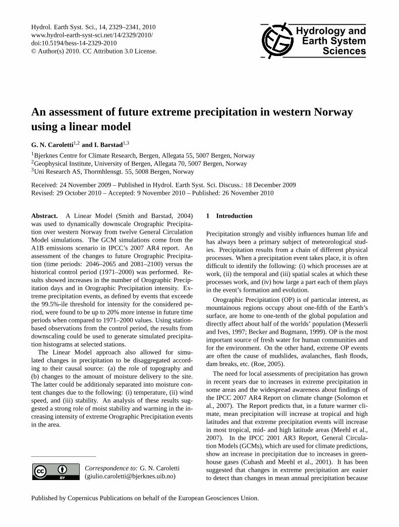
Figure 1: A schematic illustration of orographic precipitation as the result ofstable upslope ascent. Illustration by Marco Caradonna, 2009, based on a �gurefrom Roe, 2005.

23

Fig. 1. A schematic illustration of orographic precipitationas the result of stable upslope ascent. Illustration by MarcoCaradonna (2009), based on a figure from Roe (2005).

Applying simple algebra, an expression for the Fouriertransform of the precipitation distributionP is obtained, asfollows:

P (k,l) =S(k,l)

(1 + i σ τc) (1 + i σ τf), (5)

which is dependent on the sourceS(x,y) and considers timedelays (the conversion and fall-out termsτc andτf).

Combining Eqs. (2) and (5) yields a “transfer function”relating the Fourier transform of the terrainh and the precip-itation fieldP :

P (k,l) =CW i σ h(k,l)

(1 − i m HW) (1 + i σ τc) (1 + i σ τf), (6)

in which the denominator’s factors represent airflow dynam-ics (first term), cloud delays and advection (second and thirdterms, respectively).

The precipitation distribution is then obtained with the useof an inverse Fourier transform

P(x,y) =

∫∞

−∞

∫∞

−∞

P (k,l) ei(kx+ly) dkdl. (7)

www.hydrol-earth-syst-sci.net/14/2329/2010/ Hydrol. Earth Syst. Sci., 14, 2329–2341, 2010


In short, the LM describes the effect of orography andmean wind on precipitation, and, with some complexity, theeffects of temperature, humidity, moist stability, conversionand fallout times of hydrometeors.

Source term breakdown

LM can also be used to understand the mechanisms behinddownscaled changes in OP extremes.

From now on, we will useN = Nm, T = Tref.Smith and Barstad (2004) have shown that the moisture

influx magnitude (F ) depends on saturation water vapourdensity at the groundρSref(T ), water vapour scale heightHW(N,T ) and wind speedU :

F = ρSref HW U. (8)

There is a linear relationship between the moist air influxand the precipitation in LM: by comparing Eqs. (1) and (8)we get:

S =F

HW

0m

γ∇ h(x,y) = ρSref U

0m

γ∇ h(x,y). (9)

By using the relationship between lapse rates and moiststatic stability (Fraser et al., 1973)N2

= gγ−0m

Tand remem-

bering thatHW = −R T 2

Lγwe get:

0m = γ −N2 T

g(10)

γ = −RT 2

LHW.

Thus:

S = ρSref U

[N2 HW L

gRT+ 1

]∇ h(x,y). (11)

Notwithstanding the orography, the change in the sourceterm will be fully determined by the change in temperature,stability and wind magnitude: to establish their influence onthe source, we calculate the source term in Eq. (11) by vary-ing only one of the variables at a time. A mixing term ofT andN2, that comes from the fact thatHW = HW(N,T ),remains unaccounted for, but it is shown to be small.

3 Downscaling GCMs

The use of LM for downscaling may help to bridge the gapbetween poorly resolved GCM data and the need for detailedprecipitation data. Variables and parameters used for inputin the LM are shown in Table 2. GCMs’ precipitation outputhas not been used. Precipitation intensity was calculated inmm/day.

21 models were used for A1B scenario testing, for a to-tal of 41 model runs. Not all of them were available dueto incomplete data sets or other inconsistencies that could

Table 2. Model inputs.

Input Variable Symbol Data Source

Wind U GCM dataTemperature T GCM dataMoist static stability Nm GCM dataHumidity q GCM dataRelative humidity RH GCM dataTerrain h DEM topographyConversion time τc User defined as 1000 sFallout time τf User defined as 1000 sBackground precipitation – User defined as 0 mm h−1

affect the plausibility of the final results. Those with miss-ing data were dismissed, as were those showing unreason-able predictions for temperature in western Norway (annualaverage temperature between 40◦C and 0◦C). Our final se-lection is based on 12 simulations from 10 GCMs (Table 3).By using an ensemble mean, the trends in precipitation andextreme event intensity are not hidden by the annual variabil-ity in individual model runs.

The A1B scenario provides daily data for horizontal wind(U,V ), temperatureT and moist stability frequencyNm.These are constant mean values for the whole domain, andare updated daily. Conversion and fallout times were setto 1000 s. Typical conversion times are between 200 s and2000 s (Smith, 2003); longer residence times within cloudsresult in precipitation delay. The time delayτ = 1000 s valueswere not expected to be exact, but generally summarised thecombined effects of many cloud physics processes (Barstadand Smith, 2005), and have been used in LM for studies atthe regional scale (Smith, 2006; Crochet et al., 2007). Longertime delays typically result in more precipitation being ad-vected past regions of steep topography, increased precipita-tion on the lee side of the topography and lower overall pre-cipitation intensity. Conversely, shorter time delays result inmore intense rain being shifted upwind (Smith and Barstad,2004; Barstad et al., 2007).

The LM’s grid corresponds to the Digital ElevationModel (DEM) GTOPO30 topography grid, and has a reso-lution of 30”. At a latitude of 60◦, this corresponds to anaverage grid spacing of about 450 m× 900 m, which is suffi-cient to resolve important scales affecting OP.

Our first step was to identify OP events. The only daysconsidered in our study were those with a relative humidityabove or equal to 85%. This is because lower relative hu-midities result in relatively weak to no OP (Barstad et al.,2007). In addition, only days with prevailing wind directionsbetween 180◦ and 300◦ (westerly winds) were considered, asthey are the only ones to give rise to significant OP (Barstad,2002).

The second step of the study was to identify days withextreme OP. There are several possible ways of defining an



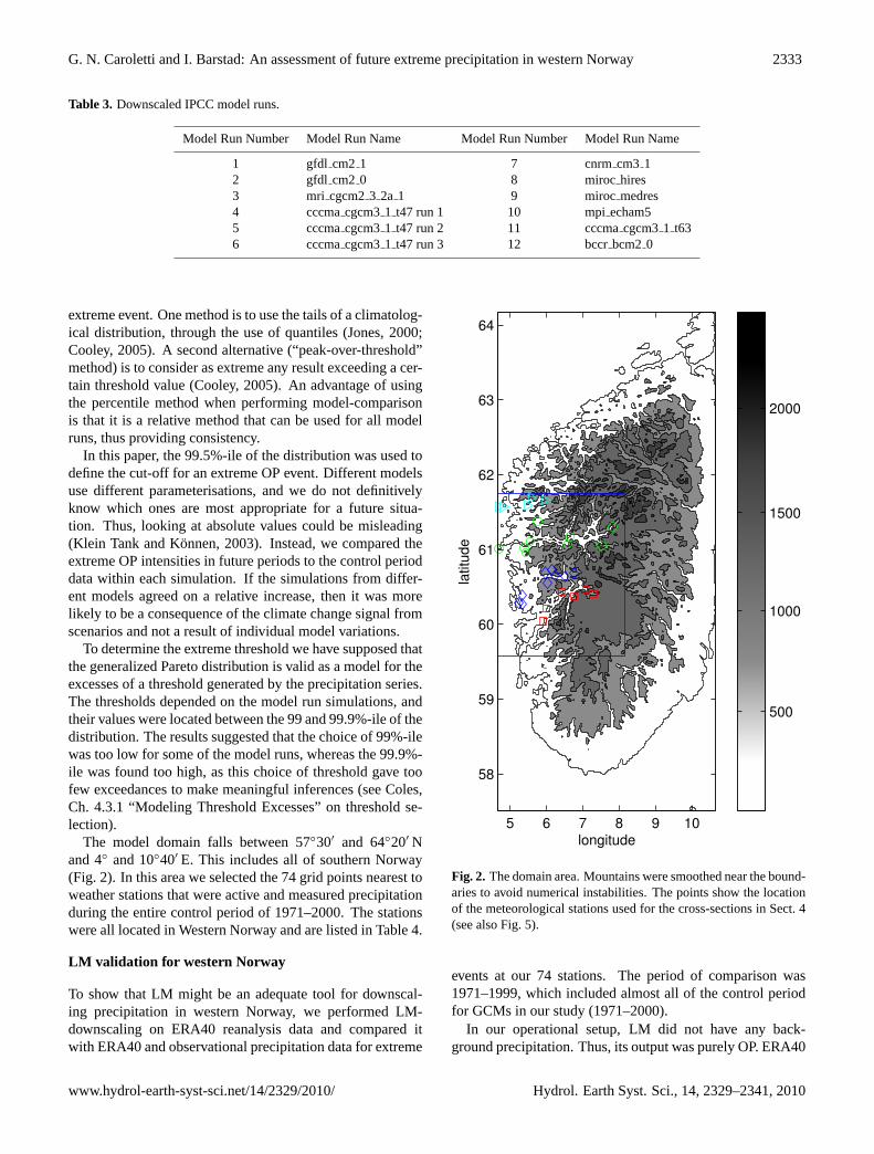
Table 3. Downscaled IPCC model runs.

Model Run Number Model Run Name Model Run Number Model Run Name

1 gfdl cm2 1 7 cnrmcm3 12 gfdl cm2 0 8 mirochires3 mri cgcm23 2a 1 9 mirocmedres4 cccmacgcm31 t47 run 1 10 mpiecham55 cccmacgcm31 t47 run 2 11 cccmacgcm31 t636 cccmacgcm31 t47 run 3 12 bccrbcm20

extreme event. One method is to use the tails of a climatolog-ical distribution, through the use of quantiles (Jones, 2000;Cooley, 2005). A second alternative (“peak-over-threshold”method) is to consider as extreme any result exceeding a cer-tain threshold value (Cooley, 2005). An advantage of usingthe percentile method when performing model-comparisonis that it is a relative method that can be used for all modelruns, thus providing consistency.

In this paper, the 99.5%-ile of the distribution was used todefine the cut-off for an extreme OP event. Different modelsuse different parameterisations, and we do not definitivelyknow which ones are most appropriate for a future situa-tion. Thus, looking at absolute values could be misleading(Klein Tank and Konnen, 2003). Instead, we compared theextreme OP intensities in future periods to the control perioddata within each simulation. If the simulations from differ-ent models agreed on a relative increase, then it was morelikely to be a consequence of the climate change signal fromscenarios and not a result of individual model variations.

To determine the extreme threshold we have supposed thatthe generalized Pareto distribution is valid as a model for theexcesses of a threshold generated by the precipitation series.The thresholds depended on the model run simulations, andtheir values were located between the 99 and 99.9%-ile of thedistribution. The results suggested that the choice of 99%-ilewas too low for some of the model runs, whereas the 99.9%-ile was found too high, as this choice of threshold gave toofew exceedances to make meaningful inferences (see Coles,Ch. 4.3.1 “Modeling Threshold Excesses” on threshold se-lection).

The model domain falls between 57◦30′ and 64◦20′ Nand 4◦ and 10◦40′ E. This includes all of southern Norway(Fig. 2). In this area we selected the 74 grid points nearest toweather stations that were active and measured precipitationduring the entire control period of 1971–2000. The stationswere all located in Western Norway and are listed in Table 4.

LM validation for western Norway

To show that LM might be an adequate tool for downscal-ing precipitation in western Norway, we performed LM-downscaling on ERA40 reanalysis data and compared itwith ERA40 and observational precipitation data for extreme

longitude

latitu

de

5 6 7 8 9 10

58

59

60

61

62

63

64

500

1000

1500

2000

Figure 2: The domain area. Mountains were smoothed near the boundaries toavoid numerical instabilities. The points show the location of the meteorologicalstations used for the cross-sections in Section 4 (see also Fig. 5).

24

Fig. 2. The domain area. Mountains were smoothed near the bound-aries to avoid numerical instabilities. The points show the locationof the meteorological stations used for the cross-sections in Sect. 4(see also Fig. 5).

events at our 74 stations. The period of comparison was1971–1999, which included almost all of the control periodfor GCMs in our study (1971–2000).

In our operational setup, LM did not have any back-ground precipitation. Thus, its output was purely OP. ERA40



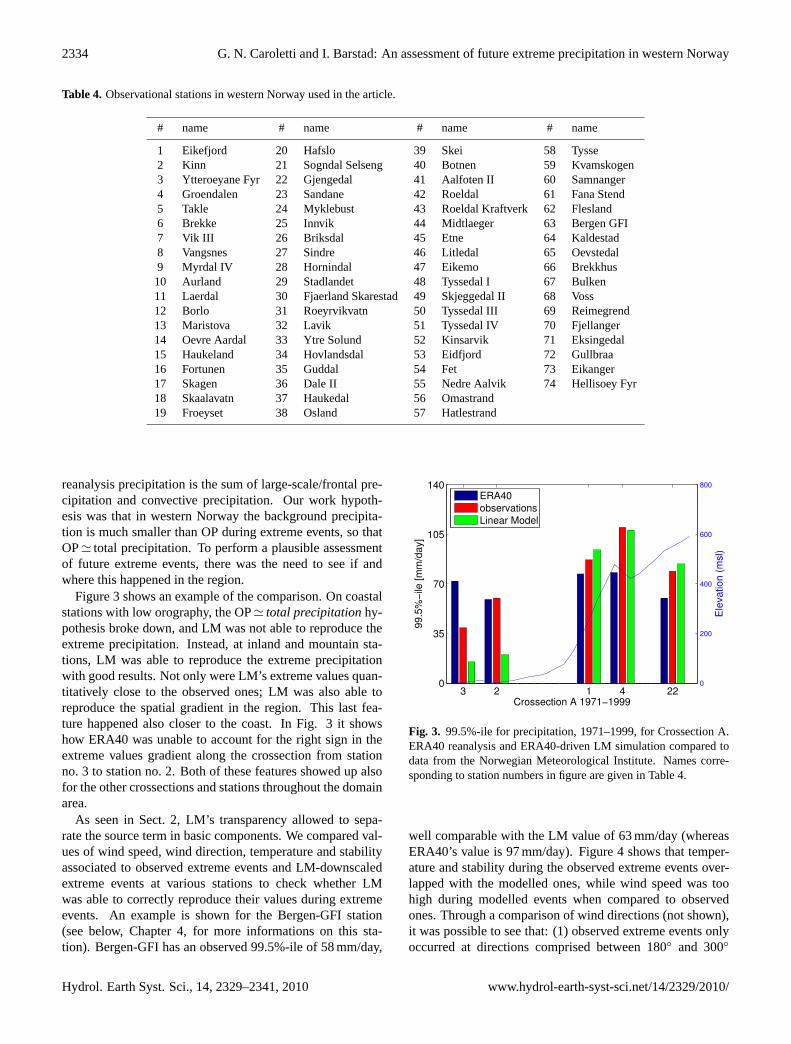
Table 4. Observational stations in western Norway used in the article.

# name # name # name # name

1 Eikefjord 20 Hafslo 39 Skei 58 Tysse2 Kinn 21 Sogndal Selseng 40 Botnen 59 Kvamskogen3 Ytteroeyane Fyr 22 Gjengedal 41 Aalfoten II 60 Samnanger4 Groendalen 23 Sandane 42 Roeldal 61 Fana Stend5 Takle 24 Myklebust 43 Roeldal Kraftverk 62 Flesland6 Brekke 25 Innvik 44 Midtlaeger 63 Bergen GFI7 Vik III 26 Briksdal 45 Etne 64 Kaldestad8 Vangsnes 27 Sindre 46 Litledal 65 Oevstedal9 Myrdal IV 28 Hornindal 47 Eikemo 66 Brekkhus10 Aurland 29 Stadlandet 48 Tyssedal I 67 Bulken11 Laerdal 30 Fjaerland Skarestad 49 Skjeggedal II 68 Voss12 Borlo 31 Roeyrvikvatn 50 Tyssedal III 69 Reimegrend13 Maristova 32 Lavik 51 Tyssedal IV 70 Fjellanger14 Oevre Aardal 33 Ytre Solund 52 Kinsarvik 71 Eksingedal15 Haukeland 34 Hovlandsdal 53 Eidfjord 72 Gullbraa16 Fortunen 35 Guddal 54 Fet 73 Eikanger17 Skagen 36 Dale II 55 Nedre Aalvik 74 Hellisoey Fyr18 Skaalavatn 37 Haukedal 56 Omastrand19 Froeyset 38 Osland 57 Hatlestrand

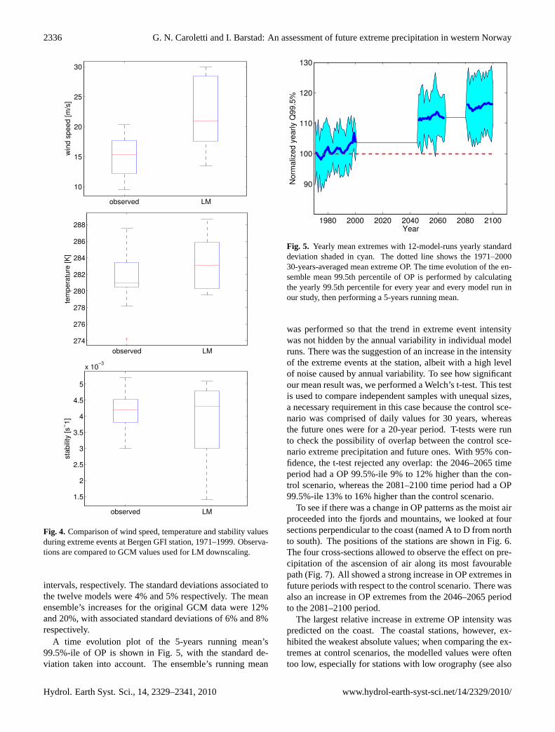
reanalysis precipitation is the sum of large-scale/frontal pre-cipitation and convective precipitation. Our work hypoth-esis was that in western Norway the background precipita-tion is much smaller than OP during extreme events, so thatOP' total precipitation. To perform a plausible assessmentof future extreme events, there was the need to see if andwhere this happened in the region.

Figure 3 shows an example of the comparison. On coastalstations with low orography, the OP' total precipitationhy-pothesis broke down, and LM was not able to reproduce theextreme precipitation. Instead, at inland and mountain sta-tions, LM was able to reproduce the extreme precipitationwith good results. Not only were LM’s extreme values quan-titatively close to the observed ones; LM was also able toreproduce the spatial gradient in the region. This last fea-ture happened also closer to the coast. In Fig. 3 it showshow ERA40 was unable to account for the right sign in theextreme values gradient along the crossection from stationno. 3 to station no. 2. Both of these features showed up alsofor the other crossections and stations throughout the domainarea.

As seen in Sect. 2, LM’s transparency allowed to sepa-rate the source term in basic components. We compared val-ues of wind speed, wind direction, temperature and stabilityassociated to observed extreme events and LM-downscaledextreme events at various stations to check whether LMwas able to correctly reproduce their values during extremeevents. An example is shown for the Bergen-GFI station(see below, Chapter 4, for more informations on this sta-tion). Bergen-GFI has an observed 99.5%-ile of 58 mm/day,

3 2 1 4 220

35

70

105

140

Crossection A 1971−1999

99

.5%

−ile

[m

m/d

ay]

0

200

400

600

800

Ele

va

tio

n (

msl)

ERA40

observations

Linear Model

Figure 3: 99.5%-ile for precipitation, 1971-1999, for Crossection A. ERA40 re-analysis and ERA40-driven LM simulation compared to data from the Norwe-gian Meteorological Institute. Names corresponding to station numbers in �gureare given in Table 4.

25

Fig. 3. 99.5%-ile for precipitation, 1971–1999, for Crossection A.ERA40 reanalysis and ERA40-driven LM simulation compared todata from the Norwegian Meteorological Institute. Names corre-sponding to station numbers in figure are given in Table 4.

well comparable with the LM value of 63 mm/day (whereasERA40’s value is 97 mm/day). Figure 4 shows that temper-ature and stability during the observed extreme events over-lapped with the modelled ones, while wind speed was toohigh during modelled events when compared to observedones. Through a comparison of wind directions (not shown),it was possible to see that: (1) observed extreme events onlyoccurred at directions comprised between 180◦ and 300◦



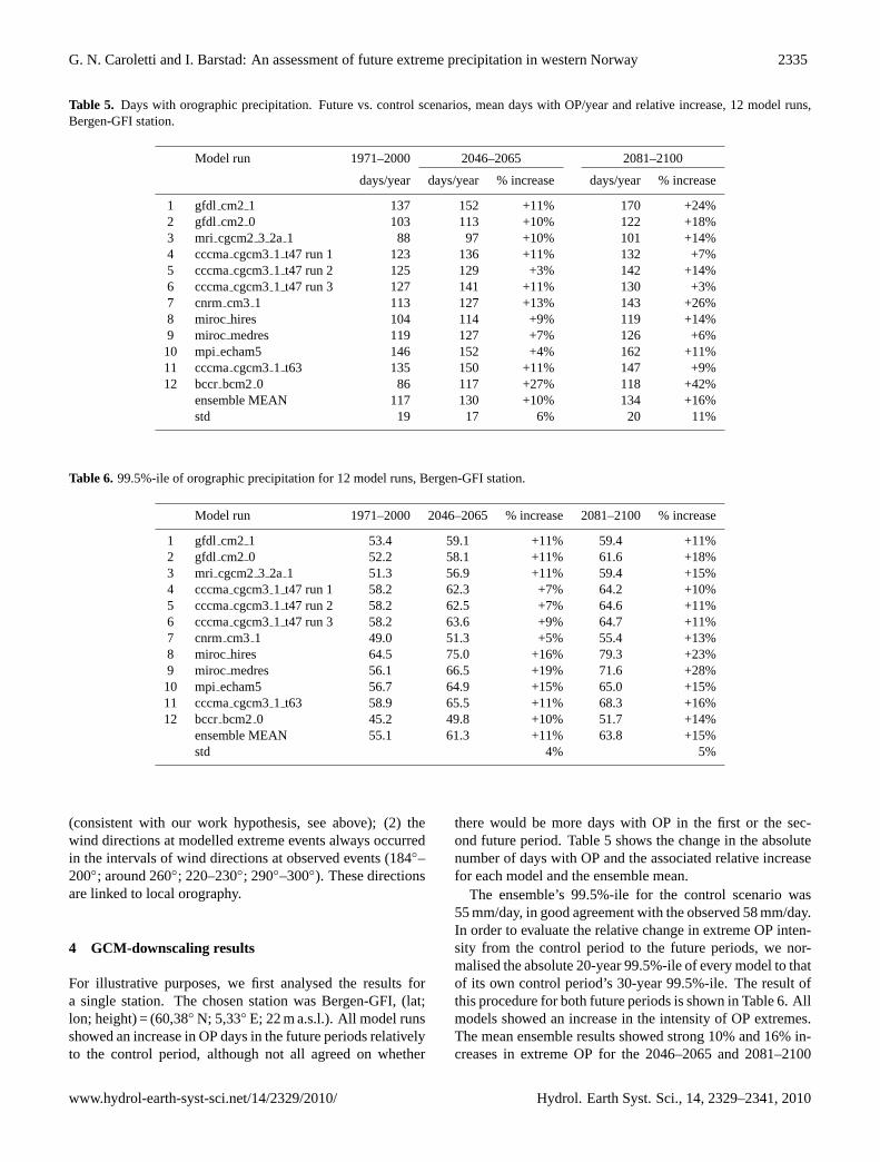
Table 5. Days with orographic precipitation. Future vs. control scenarios, mean days with OP/year and relative increase, 12 model runs,Bergen-GFI station.

Model run 1971–2000 2046–2065 2081–2100

days/year days/year % increase days/year % increase

1 gfdl cm2 1 137 152 +11% 170 +24%2 gfdl cm2 0 103 113 +10% 122 +18%3 mri cgcm23 2a 1 88 97 +10% 101 +14%4 cccmacgcm31 t47 run 1 123 136 +11% 132 +7%5 cccmacgcm31 t47 run 2 125 129 +3% 142 +14%6 cccmacgcm31 t47 run 3 127 141 +11% 130 +3%7 cnrmcm3 1 113 127 +13% 143 +26%8 miroc hires 104 114 +9% 119 +14%9 miroc medres 119 127 +7% 126 +6%10 mpi echam5 146 152 +4% 162 +11%11 cccmacgcm31 t63 135 150 +11% 147 +9%12 bccrbcm20 86 117 +27% 118 +42%

ensemble MEAN 117 130 +10% 134 +16%std 19 17 6% 20 11%

Table 6. 99.5%-ile of orographic precipitation for 12 model runs, Bergen-GFI station.

Model run 1971–2000 2046–2065 % increase 2081–2100 % increase

1 gfdl cm2 1 53.4 59.1 +11% 59.4 +11%2 gfdl cm2 0 52.2 58.1 +11% 61.6 +18%3 mri cgcm23 2a 1 51.3 56.9 +11% 59.4 +15%4 cccmacgcm31 t47 run 1 58.2 62.3 +7% 64.2 +10%5 cccmacgcm31 t47 run 2 58.2 62.5 +7% 64.6 +11%6 cccmacgcm31 t47 run 3 58.2 63.6 +9% 64.7 +11%7 cnrmcm3 1 49.0 51.3 +5% 55.4 +13%8 miroc hires 64.5 75.0 +16% 79.3 +23%9 miroc medres 56.1 66.5 +19% 71.6 +28%10 mpi echam5 56.7 64.9 +15% 65.0 +15%11 cccmacgcm31 t63 58.9 65.5 +11% 68.3 +16%12 bccrbcm20 45.2 49.8 +10% 51.7 +14%

ensemble MEAN 55.1 61.3 +11% 63.8 +15%std 4% 5%

(consistent with our work hypothesis, see above); (2) thewind directions at modelled extreme events always occurredin the intervals of wind directions at observed events (184◦–200◦; around 260◦; 220–230◦; 290◦–300◦). These directionsare linked to local orography.

4 GCM-downscaling results

For illustrative purposes, we first analysed the results fora single station. The chosen station was Bergen-GFI, (lat;lon; height) = (60,38◦ N; 5,33◦ E; 22 m a.s.l.). All model runsshowed an increase in OP days in the future periods relativelyto the control period, although not all agreed on whether

there would be more days with OP in the first or the sec-ond future period. Table 5 shows the change in the absolutenumber of days with OP and the associated relative increasefor each model and the ensemble mean.

The ensemble’s 99.5%-ile for the control scenario was55 mm/day, in good agreement with the observed 58 mm/day.In order to evaluate the relative change in extreme OP inten-sity from the control period to the future periods, we nor-malised the absolute 20-year 99.5%-ile of every model to thatof its own control period’s 30-year 99.5%-ile. The result ofthis procedure for both future periods is shown in Table 6. Allmodels showed an increase in the intensity of OP extremes.The mean ensemble results showed strong 10% and 16% in-creases in extreme OP for the 2046–2065 and 2081–2100



observed LM

10

15

20

25

30w

ind

sp

ee

d [

m/s

]

observed LM

274

276

278

280

282

284

286

288

tem

pe

ratu

re [

K]

observed LM

1.5

2

2.5

3

3.5

4

4.5

5

x 10−3

sta

bili

ty [

s−1

]

Figure 4: Comparison of wind speed, temperature and stability values duringextreme events at Bergen GFI station, 1971-1999. Observations are comparedto GCM values used for LM downscaling.

26

observed LM

10

15

20

25

30

win

d s

pe

ed

[m

/s]

observed LM

274

276

278

280

282

284

286

288

tem

pe

ratu

re [

K]

observed LM

1.5

2

2.5

3

3.5

4

4.5

5

x 10−3

sta

bili

ty [

s−1

]


26

observed LM

10

15

20

25

30

win

d s

peed [m

/s]

observed LM

274

276

278

280

282

284

286

288

tem

pera

ture

[K

]

observed LM

1.5

2

2.5

3

3.5

4

4.5

5

x 10−3

sta

bili

ty [s

−1]


26

Fig. 4. Comparison of wind speed, temperature and stability valuesduring extreme events at Bergen GFI station, 1971–1999. Observa-tions are compared to GCM values used for LM downscaling.

intervals, respectively. The standard deviations associated tothe twelve models were 4% and 5% respectively. The meanensemble’s increases for the original GCM data were 12%and 20%, with associated standard deviations of 6% and 8%respectively.

A time evolution plot of the 5-years running mean’s99.5%-ile of OP is shown in Fig. 5, with the standard de-viation taken into account. The ensemble’s running mean

1980 2000 2020 2040 2060 2080 2100

90

100

110

120

130

Year

Norm

aliz

ed y

early Q

99.5

%

Figure 5: Yearly mean extremes with 12-model-runs yearly standard deviationshaded in cyan. The dotted line shows the 1971-2000 30-years-averaged meanextreme OP. The time evolution of the ensemble mean 99.5th percentile of OPis performed by calculating the yearly 99.5th percentile for every year and everymodel run in our study, then performing a 5-years running mean.

27

Fig. 5. Yearly mean extremes with 12-model-runs yearly standarddeviation shaded in cyan. The dotted line shows the 1971–200030-years-averaged mean extreme OP. The time evolution of the en-semble mean 99.5th percentile of OP is performed by calculatingthe yearly 99.5th percentile for every year and every model run inour study, then performing a 5-years running mean.

was performed so that the trend in extreme event intensitywas not hidden by the annual variability in individual modelruns. There was the suggestion of an increase in the intensityof the extreme events at the station, albeit with a high levelof noise caused by annual variability. To see how significantour mean result was, we performed a Welch’s t-test. This testis used to compare independent samples with unequal sizes,a necessary requirement in this case because the control sce-nario was comprised of daily values for 30 years, whereasthe future ones were for a 20-year period. T-tests were runto check the possibility of overlap between the control sce-nario extreme precipitation and future ones. With 95% con-fidence, the t-test rejected any overlap: the 2046–2065 timeperiod had a OP 99.5%-ile 9% to 12% higher than the con-trol scenario, whereas the 2081–2100 time period had a OP99.5%-ile 13% to 16% higher than the control scenario.

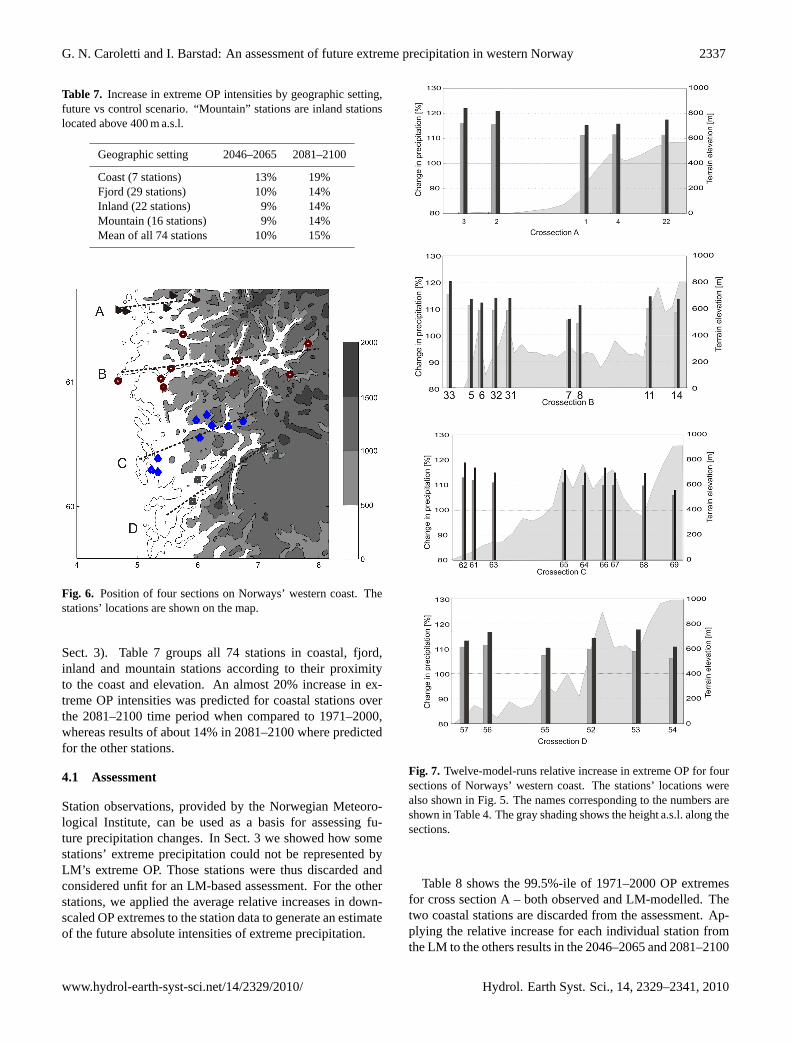
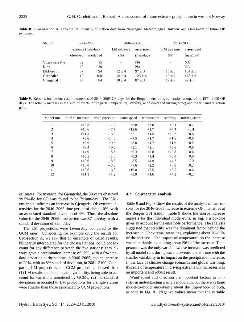
To see if there was a change in OP patterns as the moist airproceeded into the fjords and mountains, we looked at foursections perpendicular to the coast (named A to D from northto south). The positions of the stations are shown in Fig. 6.The four cross-sections allowed to observe the effect on pre-cipitation of the ascension of air along its most favourablepath (Fig. 7). All showed a strong increase in OP extremes infuture periods with respect to the control scenario. There wasalso an increase in OP extremes from the 2046–2065 periodto the 2081–2100 period.

The largest relative increase in extreme OP intensity waspredicted on the coast. The coastal stations, however, ex-hibited the weakest absolute values; when comparing the ex-tremes at control scenarios, the modelled values were oftentoo low, especially for stations with low orography (see also



Table 7. Increase in extreme OP intensities by geographic setting,future vs control scenario. “Mountain” stations are inland stationslocated above 400 m a.s.l.

Geographic setting 2046–2065 2081–2100

Coast (7 stations) 13% 19%Fjord (29 stations) 10% 14%Inland (22 stations) 9% 14%Mountain (16 stations) 9% 14%Mean of all 74 stations 10% 15%

Figure 6: Position of four sections on Norway's western coast. The stations'locations are shown on the map.

28

Fig. 6. Position of four sections on Norways’ western coast. Thestations’ locations are shown on the map.

Sect. 3). Table 7 groups all 74 stations in coastal, fjord,inland and mountain stations according to their proximityto the coast and elevation. An almost 20% increase in ex-treme OP intensities was predicted for coastal stations overthe 2081–2100 time period when compared to 1971–2000,whereas results of about 14% in 2081–2100 where predictedfor the other stations.

4.1 Assessment

Station observations, provided by the Norwegian Meteoro-logical Institute, can be used as a basis for assessing fu-ture precipitation changes. In Sect. 3 we showed how somestations’ extreme precipitation could not be represented byLM’s extreme OP. Those stations were thus discarded andconsidered unfit for an LM-based assessment. For the otherstations, we applied the average relative increases in down-scaled OP extremes to the station data to generate an estimateof the future absolute intensities of extreme precipitation.

Fig. 7. Twelve-model-runs relative increase in extreme OP for foursections of Norways’ western coast. The stations’ locations werealso shown in Fig. 5. The names corresponding to the numbers areshown in Table 4. The gray shading shows the height a.s.l. along thesections.

Table 8 shows the 99.5%-ile of 1971–2000 OP extremesfor cross section A – both observed and LM-modelled. Thetwo coastal stations are discarded from the assessment. Ap-plying the relative increase for each individual station fromthe LM to the others results in the 2046–2065 and 2081–2100



Table 8. Cross-section A. Extreme OP intensity of station data from Norwegian Meteorological Institute and assessment of future OPextremes.

Station 1971–2000 2046–2065 2081–2000

extreme (mm/day) LM increase assessment LM increase assessment

observed modelled (%) (mm/day) (%) (mm/day)

Ytterøyane Fyr 39 15 – NA – NAKinn 60 20 – NA – NAEikfjord 87 94 12± 4 97± 3 16± 6 101± 5Grøndalen 110 108 12± 4 123± 4 16± 7 128± 8Gjengedal 79 84 10± 4 87± 3 17± 7 92± 6

Table 9. Reasons for the increase in extremes of 2046–2065 OP days for the Bergen meteorological station compared to 1971–2000 OPdays. The total % increase is the sum of the % influx parts (temperature, stability, windspeed and mixing error) and the % wind directionpart.

Model run Total % increase wind direction wind speed temperature stability mixing error

1 +10.8 −1.2 +3.8 +2.0 +6.1 +0.12 +10.6 −7.7 +12.6 +1.7 +4.4 −0.43 +11.3 −5.3 +2.1 +1.5 +12.2 +0.84 +6.6 +14.0 −7.5 +1.7 −1.6 +0.05 +6.6 +0.6 +3.0 +1.7 +1.6 +0.56 +9.4 +0.0 +3.1 +2.1 +3.6 +0.67 +4.9 −18.6 +9.3 +0.8 +12.8 +0.68 +16.5 +11.8 +0.3 +4.4 +0.0 +0.09 +19.0 +18.6 −8.5 +4.9 +4.2 −0.210 +15.0 −3.0 +7.6 +2.2 +8.0 +0.211 +10.6 −6.0 +10.0 +2.5 +3.5 +0.612 +11.1 +1.2 +3.9 +1.6 +4.2 +0.2

estimates. For instance, for Gjengedal, the 30 years observed99.5%-ile for OP was found to be 79 mm/day. The LM-ensemble indicates an increase in Gjengedal OP extreme in-tensities for the 2046–2065 time period of about 10%, withan associated standard deviation of 4%. Thus, the absolutevalue for the 2046–2065 time period was 87 mm/day, with astandard deviation of 3 mm/day.

The LM projections were favourably compared to theGCM ones. Considering for example only the results forCrossection A, we saw that an ensemble of GCM results,bilinearily interpolated for the chosen stations, could not ac-count for any difference between the five stations: they al-ways gave a precipitation increase of 12%, with a 6% stan-dard deviation at the stations in 2046–2065; and an increaseof 20%, with an 8% standard deviation, in 2081–2100. Com-paring LM projections and GCM projections showed that:(1) LM results had better spatial variability, being able to ac-count for variations unnoticed by GCMs; (2) the standarddeviations associated to LM projections for a single stationwere smaller than those associated to GCM projections.

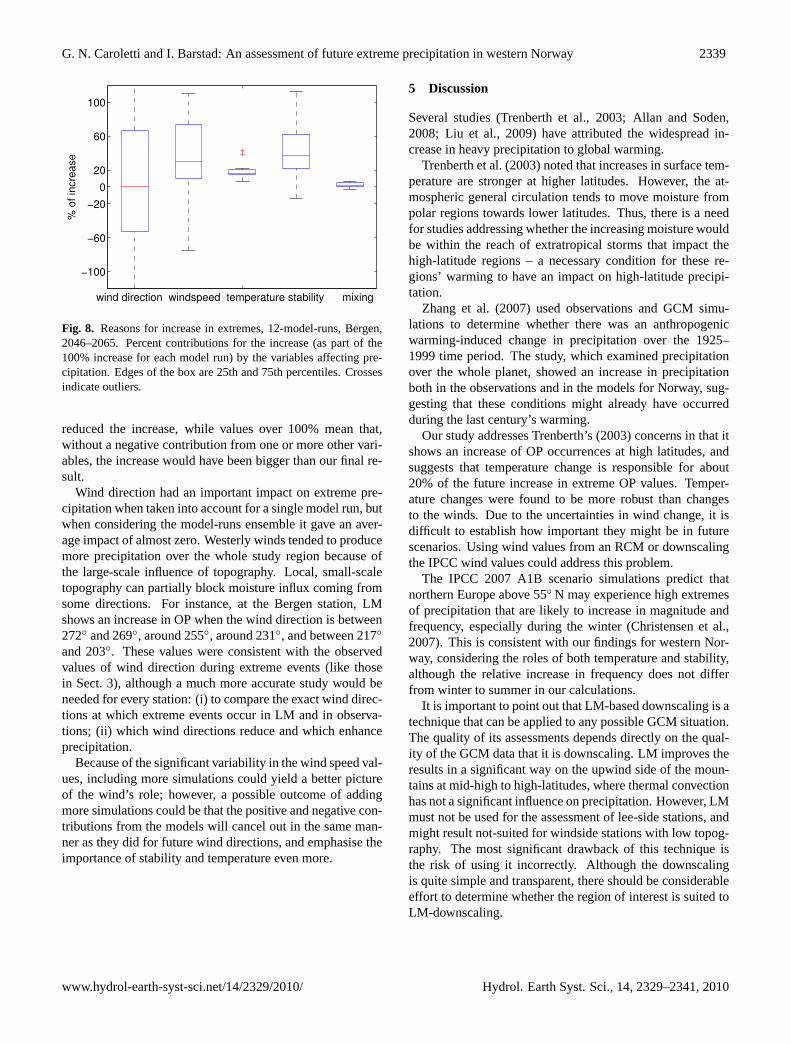
4.2 Source term analysis

Table 9 and Fig. 8 show the results of the analysis of the rea-sons for the 2046–2065 increase in extreme OP intensities atthe Bergen GFI station. Table 9 shows the source increaseanalysis for the individual model-runs; in Fig. 8 a boxplotgives an account for the ensemble performance. The analysissuggested that stability was the dominant factor behind theincrease in OP extreme intensities, explaining about 20–60%of the increase. The impact of temperature on the increasewas remarkable, explaining about 20% of the increase. Tem-perature was the only variable whose increase was predictedby all model runs during extreme events, and the one with thesmaller variability in its impact on the precipitation increase.In the face of climate change scenarios and global warming,this role of temperature in driving extreme OP increases wasan important and robust result.

Wind speed and direction are important factors to con-sider in understanding a single model run, but there was largemodel-to-model uncertainty about the importance of both,as seen in Fig. 8. Negative values mean that the variable



Figure 8: Reasons for increase in extremes, 12-model-runs, Bergen, 2046-2065.Percent contributions for the increase (as part of the 100% increase for eachmodel run) by the variables a�ecting precipitation. Edges of the box are 25thand 75th percentiles. Crosses indicate outliers.

wind direction windspeed temperature stability mixing

−100

−60

−20

0

20

60

100

% o

f in

cre

ase

30

Fig. 8. Reasons for increase in extremes, 12-model-runs, Bergen,2046–2065. Percent contributions for the increase (as part of the100% increase for each model run) by the variables affecting pre-cipitation. Edges of the box are 25th and 75th percentiles. Crossesindicate outliers.

reduced the increase, while values over 100% mean that,without a negative contribution from one or more other vari-ables, the increase would have been bigger than our final re-sult.

Wind direction had an important impact on extreme pre-cipitation when taken into account for a single model run, butwhen considering the model-runs ensemble it gave an aver-age impact of almost zero. Westerly winds tended to producemore precipitation over the whole study region because ofthe large-scale influence of topography. Local, small-scaletopography can partially block moisture influx coming fromsome directions. For instance, at the Bergen station, LMshows an increase in OP when the wind direction is between272◦ and 269◦, around 255◦, around 231◦, and between 217◦

and 203◦. These values were consistent with the observedvalues of wind direction during extreme events (like thosein Sect. 3), although a much more accurate study would beneeded for every station: (i) to compare the exact wind direc-tions at which extreme events occur in LM and in observa-tions; (ii) which wind directions reduce and which enhanceprecipitation.

Because of the significant variability in the wind speed val-ues, including more simulations could yield a better pictureof the wind’s role; however, a possible outcome of addingmore simulations could be that the positive and negative con-tributions from the models will cancel out in the same man-ner as they did for future wind directions, and emphasise theimportance of stability and temperature even more.

5 Discussion

Several studies (Trenberth et al., 2003; Allan and Soden,2008; Liu et al., 2009) have attributed the widespread in-crease in heavy precipitation to global warming.

Trenberth et al. (2003) noted that increases in surface tem-perature are stronger at higher latitudes. However, the at-mospheric general circulation tends to move moisture frompolar regions towards lower latitudes. Thus, there is a needfor studies addressing whether the increasing moisture wouldbe within the reach of extratropical storms that impact thehigh-latitude regions – a necessary condition for these re-gions’ warming to have an impact on high-latitude precipi-tation.

Zhang et al. (2007) used observations and GCM simu-lations to determine whether there was an anthropogenicwarming-induced change in precipitation over the 1925–1999 time period. The study, which examined precipitationover the whole planet, showed an increase in precipitationboth in the observations and in the models for Norway, sug-gesting that these conditions might already have occurredduring the last century’s warming.

Our study addresses Trenberth’s (2003) concerns in that itshows an increase of OP occurrences at high latitudes, andsuggests that temperature change is responsible for about20% of the future increase in extreme OP values. Temper-ature changes were found to be more robust than changesto the winds. Due to the uncertainties in wind change, it isdifficult to establish how important they might be in futurescenarios. Using wind values from an RCM or downscalingthe IPCC wind values could address this problem.

The IPCC 2007 A1B scenario simulations predict thatnorthern Europe above 55◦ N may experience high extremesof precipitation that are likely to increase in magnitude andfrequency, especially during the winter (Christensen et al.,2007). This is consistent with our findings for western Nor-way, considering the roles of both temperature and stability,although the relative increase in frequency does not differfrom winter to summer in our calculations.

It is important to point out that LM-based downscaling is atechnique that can be applied to any possible GCM situation.The quality of its assessments depends directly on the qual-ity of the GCM data that it is downscaling. LM improves theresults in a significant way on the upwind side of the moun-tains at mid-high to high-latitudes, where thermal convectionhas not a significant influence on precipitation. However, LMmust not be used for the assessment of lee-side stations, andmight result not-suited for windside stations with low topog-raphy. The most significant drawback of this technique isthe risk of using it incorrectly. Although the downscalingis quite simple and transparent, there should be considerableeffort to determine whether the region of interest is suited toLM-downscaling.



6 Summary

In this study, an efficient downscaling method, Smithand Barstad’s Linear Model (2004), was used to physi-cally downscale precipitation from 12 model runs of theIPCC 2007 A1B scenario over western Norway. The resultsshowed an increase in Orographic Precipitation (OP) occur-rence and an increase in the intensity of OP extremes over74 grid points corresponding to Norwegian weather stations.The increase in intensity was found to be around 10% ofthe absolute values for the 2046–2065 scenario and around15% for the 2081–2100 scenario, consistently with the gen-eral GCMs results. However, the improved resolution of LMallowed to perform an assessment of absolute future changesto extreme OP, based on the relative increase of the modelresults and on weather station observations.

The main reason for the increase of precipitation wasmore closely investigated for the Bergen meteorologicalstation. The increase in moist air influx contributed sig-nificantly, whereas the contribution of wind direction wasstrongly model-dependent and tended to naught when model-averaged. By separating out the factors that contributed tothe source term, the results showed that stability and temper-ature increases were likely to be the main cause of increasedinflux, with temperature accounting for roughly 20% of theintensity increase in extreme OP for all models.

The present paper was meant as an introduction to pos-sible uses of analysis connected to LM downscaling andshowed methods that can be generally applied to many dif-ferent model simulations.

Downscaling climate scenarios with LM seems to open upinteresting possibilities for insight. In climatology, for in-stance, it can be used as a tool to evaluate GCM performancein the following areas:

i. The use of standard deviations of relative values insteadof absolute ones makes it easier to compare models andpoint out those that may be underperforming;

ii. the transparent nature of LM makes it easy to see inwhich respect the models diverge and what impact thathas on the downscaled results.

In weather forecasting, LM downscaling can be useful forpresent and future studies. Some examples include the fol-lowing:

i. For the present by providing informations on how somevariables can influence moist air influx, that might havebeen overlooked;

ii. for the future, because LM downscaling points out howthe relationship of these variables to precipitation mightchange and indicates which variables have to be moni-tored in case need should arise to change the parameter-isation and settings of the forecasting models.

Acknowledgements.This is publication no. A311 from the Bjerk-nes Centre for Climate Research.

The USGS 30 ARC-second Global Elevation Data, GTOPO30, arefrom the Research Data Archive (RDA), which is maintained bythe Computational and Information Systems Laboratory (CISL) atthe National Center for Atmospheric Research (NCAR). NCAR issponsored by the National Science Foundation (NSF). The origi-nal data are available from the RDA (http://dss.ucar.edu) in datasetnumber ds758.0.

Many thanks to Jurgen Bader, Justin Wettstein and Anna Fitch fortheir valuable comments on the manuscript.

We also wish to thank Natascha Topfer and the HESS EditorialBoard, and the Editor, Jan Seibert, for their input, and the anony-mous reviewers for their careful and attentive comments that helpedto improve the scientific value of this paper.

Edited by: J. Seibert

References

Allan, R. P. and Soden, B. J.: Atmospheric Warming and theAmplification of Precipitation Extremes, Science, 321, 5895,doi:10.1126/science.1160787, 2008.

Andersen, P.: The distribution of monthly precipitation in South-ern Norway in relation to prevailing H. Johansen weather types,Arbok Universitet Bergen, Mat. Naturv. Ser., 1972(1), 1–20,1973.

Andersen, P.: Surface winds in southern Norway in relation to pre-vailing H. Johansen weather types, Meteorol. Ann., 6(14), 377–399, 1975.

Barstad, I.: Southwesterly flows over southern Norway, Reports inmeteorology and oceanography 7, Geofysisk Institutt, UiB, Doc-toral Thesis, 2002.

Barstad, I. and Smith, R. B.: Evaluation of an Orographic Precipi-tation Model, J. Hydrometeorol., 6, 85–99, 2005.

Barstad, I., Grabowski, W. W., and Smolarkiewicz, P. K.: Charac-teristics of large-scale orographic precipitation, J. Hydrol., 340,78–90, 2007.

Barstad, I., Sorteberg, A., Flatøy, F., and Deque, M.: Precipita-tion, temperature and wind in Norway: dynamical downscalingof ERA40, Clim. Dynam., 33, 769–776, 2008.

Becker, M. and Bugmann, H.: Global Change and Mountain Re-gions – The Mountain Research Initiative, Global Terrestrial Ob-serving System, Report n. 28, 1999.

Bousquet, O. and Smull, B. F.: Comparative study of twoorographic precipitation events exhibiting significant upstreamblocking during MAP, in Extended abstracts from the MAPmeeting 2001, MAP Newsletter 15, 2001.

Christensen, J. H., Hewitson, B., Busuioc, A., Chen, A., Gao,X., Held, I., Jones, R., Kolli, R. K., Kwon, W.-T., Laprise, R.,Magana Rueda, V., Mearns., L., Menendez, C. G., Raisanen, J.,Rinke, A., Sarr, A., and Whetton, P.: Regional Climate Projec-tions, in: Climate Change 2007: The Physical Science Basis,Contribution of Working Group I to the Fourth Assessment Re-port of the Intergovernmental Panel on Climate Change, editedby: Solomon, S., Qin, D., Manning, M., Chen, Z., Marquis, M.,Averyt, K. B., Tignor, M., and Miller, H. L., Cambridge Univer-sity Press, Cambridge, UK and New York, NY, USA, 2007.


http://dss.ucar.edu


Coles, S.: An introduction to statistical modeling of extreme values,Springer, London, 2001.

Cooley, D. S.: Statistical Analysis of Extremes Motivated byWeather and Climate Studies: Applied and Theoretical Ad-vances, Doctoral Thesis, University of Colorado at Boulder, De-partment of Applied Mathematics, 1–122, 2005.

Coppola, E. and Giorgi, F.: Climate change in tropical regions fromhigh resolution time slice AGCM experiments, Q. J. Roy. Meteor.Soc., 131B, 3123–3146, 2005.

Crochet, P., Johannesson, T., Jonsson, T., Sigurdsson, O., Bjorns-son, H., Palsson, F., and Barstad I.: Estimating the Spatial Distri-bution of Precipitation in Iceland Using a Linear Model of Oro-graphic Precipitation, J. Hydrometeorol., 8, 1285–1306, 2007.

Cubasch, U., Meehl, G. A., Boer, G. J., et al.: Projections of FutureClimate Change, in: Climate Change 2001: The Scientific Basis,Contribution of Working Group I to the Third Assessment Re-port of the Intergovernmental Panel on Climate Change, editedby: Houghton, J. T., Ding, Y., Griggs, D. J., et al., CambridgeUniversity Press, 2001.

Deque, M. and Piedelievre, J. P.: High-Resolution climate simula-tion over Europe, Clim. Dynam., 11, 321–339, 1995.

Georgis, J.-F., Roux, F., Chong, M., and Pradier, S.: Triple-Dopplerradar analysis of the heavy rain event observed in the Lago Mag-giore region during MAP IOP 2b, Q. J. Roy. Meteor. Soc., 129,495–522, 2003.

Giorgi, F. and Mearns, L. O.: Introduction to special section: Re-gional climate modeling revisited, J. Geophys. Res., 104, 6335–6352, 1999.

Groisman, P., Knight, R. W., Easterling, D. R., Karl, T. K., Hegerl,G., and Razuvaev, V. N.: Trends in Intense Precipitation in theClimate Record, J. Climate, 18, 1326–1350, 2005.

Haylock, M. R., Cawley, G. C., Harpham, C., Wilby, R. L., andGoodess, C. M.: Downscaling Heavy Precipitation over theUnited Kingdom: A comparison of dynamical and statisticalmethods and their future scenarios, Int. J. Climatol., 26, 1397–1415, 2006.

Jones, C.: Occurrence of Extreme Precipitation Events in Califor-nia and Relationships with the Madden-Julian Oscillation, J. Cli-mate, 13, 3576–3587, 2000.

Klein Tank, A. M. G. and Konnen, G. P.: Trends in Indices of DailyTemperature and Precipitation Extremes in Europe, 1946–1999,J. Climate, 16, 3665–3680, 2003.

Liu, S. C., Fu, C., Shiu, C.-J., Chen, J.-P., and Wu, F.: Tempera-ture dependence of global precipitation extremes, Geophys. Res.Lett., 36, L17702, doi:10.1029/2009GL040218, 2009.

Maraun, D., Wetterhall, F., Ireson, A. M., Chandler, R. E., Kendon,E. J., Widmann, M., Brienen, S., Rust, H. W., Sauter, T., The-meßl, M., Venema, V. K. C., Chun, K. P., Goodess, C. M., Jones,R. G., Onof, C., Vrac, M., Thiele-Eich, I.: Precipitation down-scaling under climate change. Recent developments to bridge thegap between dynamical models and the end user, Rev. Geophys.,in press, doi:10.1029/2009RG000314, 2010.

Meehl, G. A., Stocker, T. F., Collins, W. D., Friedlingstein, P., Gaye,A. T., Gregory, J. M., Kitoh, A., Knutti, R., Murphy, J. M., Noda,A., Raper, S. C. B., Watterson, I. G., Weaver, A. J., and Zhao,Z.-C.: Global Climate Projections, in: Climate Change 2007:The Physical Science Basis, Contribution of Working Group I tothe Fourth Assessment Report of the Intergovernmental Panel onClimate Change, edited by: Solomon, S., Qin, D., Manning, M.,

Chen, Z., Marquis, M., Averyt, K. B., Tignor, M., and Miller, H.L., Cambridge University Press, Cambridge, UK and New York,NY, USA, 2007.

Messerli, B. and Ives, J. D.: Mountains of the World: A GlobalPriority, Parthenon Pub. Group, New York, USA, 495 pp., 1997.

Murphy, J.: An evaluation of statistical and dynamical tech-niques for downscaling local climate, J. Climate, 12(8), 2256–2284.1999.

Roe, G.: Orographic Precipitation, Annu. Rev. Earth Pl. Sc., 33,645–671, 2005.

Rotunno, R. and Ferretti, R.: Orographic effects on rainfall in MAPcases IOP 2b and IOP 8, Q. J. Roy. Meteor. Soc., 129, 373–390,2003.

Salathe Jr., E. P.: Downscaling simulations of future global climatewith application to hydrologic modelling, Int. J. Climatol., 25,419–436, 2005.

Schmidli, J., Goodess, C. M., Frei, C., Haylock, M. R., Hundecha,Y., Ribalaygua, J., and Schmith, T.: Statistical and dynamicaldownscaling of precipitation: An evaluation and comparison ofscenarios for the European Alps, J. Geophys. Res., 112, 1–20,2007.

Smith, R. B.: The influence of mountains on the atmosphere, Adv.Geophys., 21, 87–230, 1979.

Smith, R. B.: A linear upslope-time-delay model for orographicprecipitation, J. Hydrol., 282, 2–9, 2003.

Smith, R. B.: Progress on the theory of orographic precipitation,Geological Society of America, Special Paper, 398, 1–16, 2006.

Smith, R. B. and Barstad, I.: A linear theory of orographic precipi-tation, J. Atmos. Sci., 61, 1377–1391, 2004.

Solomon, S., Qin, D., Manning, M., Chen, Z., Marquis, M., Averyt,K. B., Tignor, M., and Miller, H. L.: Contribution of WorkingGroup I to the Fourth Assessment Report of the Intergovernmen-tal Panel on Climate Change, 2007, Cambridge University Press,Cambridge, UK and New York, NY, USA, 2007.

Trenberth, K. E., Dai, A., Rasmussen, R. M., and Parsons, D. B.:The changing character of precipitation, B. Am. Meteorol. Soc.,84, 1205–1217, 2003.

Wang, Y., Leung, L. R., McGregor, J. L., Lee, D. K., Wang, W. C.,Ding, Y., and Kimura, F.: Regional climate modeling: progress,challenges and prospects, J. Meteorol. Soc. Jpn., 82(6), 1599–1628, 2004.

Wilby, R. L. and Wigley, T. M. L.: Downscaling general circulationmodel output: A reappraisal of methods and limitations. In Cli-mate Prediction and Agriculture, edited by: Sivakumar, M. V. K.,Proceedings of the START/WMO International Workshop, 27–29 September 1999, Geneva, International START Secretariat,Washington, DC, 39–68, 2000.

Wilby, R. L., Wigley, T. M. L., Conway, D., Jones, P. D., Hewitson,B. C., Main, J., and Wilks, D. S.: Statistical downscaling of gen-eral circulation model output: A comparison of methods, WaterResour. Res., 34, 2995–3008, 1998.

Zhang, X., Zwiers, F. W., Hegerl, G. C., Lambert, F. H., Gillett, N.P., Solomon, S., Stott, P. A., and Nozawa, T.: Detection of humaninfluence on twentieth-century precipitation trends, Nature, 448,461–465, 2007.


An assessment of future extreme precipitation in western ...

Documents