An approach for probabilistic forecasting of seasonal turbidity threshold exceedance

ClickHere

for

FullArticle

An approach for probabilistic forecasting of seasonal turbiditythreshold exceedance

Erin Towler,1,2 Balaji Rajagopalan,1,3 R. Scott Summers,1 and David Yates2

Received 9 February 2009; revised 24 December 2009; accepted 27 January 2010; published 15 June 2010.

[1] Though climate forecasts offer substantial promise for improving water resourceoversight, additional tools are needed to translate these forecasts into water‐quality‐basedproducts that can be useful to water utility managers. To this end, a generalized approach isdeveloped that uses seasonal forecasts to predict the likelihood of exceeding a prescribedwater quality limit. Because manywater quality standards are based on thresholds, this studyutilizes a logistic regression technique, which employs nonparametric or “local” estimationthat can capture nonlinear features in the data. The approach is applied to a drinkingwater source in the Pacific Northwest United States that has experienced elevated turbidityvalues that are correlated with streamflow. The main steps of the approach are to (1) obtain aseasonal probabilistic precipitation forecast, (2) generate streamflow scenarios conditionalon the precipitation forecast, (3) use a local logistic regression to compute the turbiditythreshold exceedance probabilities, and (4) quantify the likelihood of turbidity exceedancecorresponding to the seasonal climate forecast. Results demonstrate that forecasts offer aslight improvement over climatology, but that representative forecasts are conservative andresult in only a small shift in total exceedance likelihood. Synthetic forecasts are includedto show the sensitivity of the total exceedance likelihood. The technique is general and couldbe applied to other water quality variables that depend on climate or hydroclimate.

Citation: Towler, E., B. Rajagopalan, R. S. Summers, and D. Yates (2010), An approach for probabilistic forecastingof seasonal turbidity threshold exceedance, Water Resour. Res., 46, W06511, doi:10.1029/2009WR007834.

1. Introduction

[2] Recent advances in climatology and computationalcapability are making the probabilistic forecasts of seasonalclimate over the United States and across the globe increas-ingly prevalent and skillful [Barnston et al., 1994; Goddardet al., 2003; Livezey and Timofeyeva, 2008]. Nevertheless,despite significant advances and potential benefits, watermanagers have been slow to incorporate forecasts into theirwater quality assessments. In addition to being deemedunreliable, several underlying institutional factors contributeto their underutilization, including system complexity andorganizational conservatism [Rayner et al., 2005]. In additionto these barriers, evidence suggests that practical uses forthese seasonal forecasts need to be identified [Rayner et al.,2005; Pagano et al., 2001] and tailored to a particular situa-tional vulnerability or local management practice [Paganoet al., 2002]. As such, efforts to integrate forecasts into sec-ondary products that are relevant to the major concerns ofwater managers have been explored [Carbone and Dow,2005], and this paper aims to complement and extend thoseefforts.

[3] Historic attempts to use climate forecasts have focusedon water quantity, with little extension to forecasting waterquality, which is understandable, since reliability has alwaysbeen a central tenet of water management. Seasonal stream-flow forecasting is a topic of widespread interest and an areaof active research [e.g., seeWood and Lettenmaier, 2006, andreferences therein]. As such, there have been several effortsto develop seasonal streamflow forecasts using large‐scaleseasonal climate information in combination with physicalhydrologic models [Wood and Lettenmaier, 2006; Hamletand Lettenmaier, 1999; Hay et al., 2002; Wood et al., 2002,2005], as well as through statistical techniques that incorpo-rate predictors from the ocean‐atmosphere and land system[Grantz et al., 2005; Regonda et al., 2006; Opitz‐Stapletonet al., 2007].[4] For drinkingwater utilities, the extension of forecasting

efforts to source water quality is valuable, since there areimplications for treatment and management decisions. This isplaying an increasingly important role as supplies becomestrained and regulations become more stringent. Therefore,understanding the variability of the influent water quantityand quality are important for efficient management of thesystem. Many drinking water treatment systems draw fromsurface water sources, including from flowing streams andreservoirs. For these sources, year‐to‐year variations in floware linked to the regional climate, mainly the precipitation(rainfall and/or snow) in the basin. There is increasing evi-dence that water quality pollutant concentrations are associ-ated with streamflow [Manczak and Florczyk, 1971; Johnson,1979; Stow and Borsuk, 2003], and this provides a good

1Department of Civil, Environmental andArchitectural Engineering,University of Colorado at Boulder, Boulder, Colorado, USA.

2National Center for Atmospheric Research, Boulder, Colorado,USA.

3Cooperative Institute for Research in Environmental Sciences,University of Colorado, Boulder, Colorado, USA.

Copyright 2010 by the American Geophysical Union.0043‐1397/10/2009WR007834

WATER RESOURCES RESEARCH, VOL. 46, W06511, doi:10.1029/2009WR007834, 2010

W06511 1 of 10

http://dx.doi.org/10.1029/2009WR007834

opportunity to extend the seasonal climate forecasts to rele-vant water quality applications.[5] Environmental and public health protection are often

established through the use of water quality thresholds thathave been set by regulatory agencies or identified as limits toparticular treatment options; hence, accurate assessment ofthreshold exceedances is an important management tool. Inthe context of total maximum daily loads (TMDLs) set fordischarges to streams and rivers, water quality violations havebeen assessed using probabilistic approaches [Borsuk et al.,2002], as well as through Bayesian techniques that combinemodel simulations with monitoring data [Qian and Reckhow,2007]. However, these methods do not provide a way toutilize seasonal climate forecast information for helping tomanage the potential for water quality threshold exceedances.[6] This work is motivated by the need for a simple and

flexible approach that can translate probabilistic seasonalclimate forecasts to predictions of seasonal water qualitythreshold exceedance. We develop a local logistic regressionmodel for seasonal water quality threshold exceedance basedon seasonal streamflow, which in turn is modeled usingseasonal climate forecasts. The logistic regression models thethreshold exceedance probability directly, and the “localaspect” of the logistic regression provides the ability tocapture any arbitrary (i.e., linear or nonlinear) relationshippresent in the data. This approach is unique and makes twosignificant contributions: first, it introduces a data‐drivenfunctional approach for water quality exceedance modeling,and second, it seamlessly integrates climate information,providing exceedance probabilities that are consistent with aseasonal climate forecast. We demonstrate this by applying itto modeling threshold exceedance of turbidity using stream-flow and seasonal climate forecast for a drinking water sourcein the Pacific Northwest United States. The description ofthe study region, data sets used, and details of the proposedapproach are presented in the following sections. Thisapproach will allow managers to take advantage of the ben-efits of improving skills in climate forecasts, thus enablingmore efficient water quality management. Furthermore, as

water managers are called to adapt to a nonstationary climate[Milly et al., 2008], such a tool can be used for long‐termplanning.

2. Case Study Description

[7] The case study that will be used to demonstrate thisapproach is the Bull Run River, which is the primary sourceof water for the Portland Water Bureau (PWB) in Oregon.PWB provides water to more than 20% of all Oregonians,including the city of Portland. The Bull Run Watershed isprotected and is a source with very high water quality,enabling PWB to meet federal drinking water standardswithout the filtration treatment process. However, historicflooding and subsequent high‐turbidity events have under-scored PWB’s vulnerability as an unfiltered source [PortlandWater Bureau, 2007]. For utilities that do not filter, one of thecriteria of the Surface Water Treatment Rule (SWTR)requires that the turbidity level prior to disinfection notto exceed 5 nephelometric turbidity units (NTU) [UnitedStates Environmental Protection Agency, 1989]. For PWB,if conditions arise that could cause an exceedance of 5 NTU,they follow procedures and make decisions based on moni-tored turbidity levels, weather patterns, antecedent conditions,and other case‐specific information to ensure compliance.When necessary, the PWB switches to their low‐turbiditysupplemental groundwater source. This groundwater sourceensures that the PWB is able to remain in compliance but ismore expensive due to pumping costs. As such, the avail-ability of skillful seasonal forecasts of turbidity exceedancecould provide additional information for management andplanning purposes.

2.1. Data

[8] The following data sets for the period of 1970–2007were used in the analysis.[9] 1. Monthly precipitation data for the Oregon Northern

Cascades region (Division 4) were obtained from the U.S.climate division data set from the NOAA‐CIRES ClimateDiagnostics Center (CDC)Web site (http://www.cdc.noaa.gov).[10] 2. Daily streamflow data for the main stem to the

drinking water source were obtained from U.S. GeologicalSurvey (USGS) Bull Run Station gage 14138850.[11] 3. Daily turbidity monitoring data from the treatment

plant headworks were obtained from PWB. The headworksare located below the two storage reservoirs on the Bull RunRiver and is the location from which the municipal drinkingwater supply is provided to the conduits that take water intothe Portland metropolitan area.[12] Where applicable in this analysis, monthly averages

and monthly maximums were calculated from the daily data.

2.2. Diagnostics

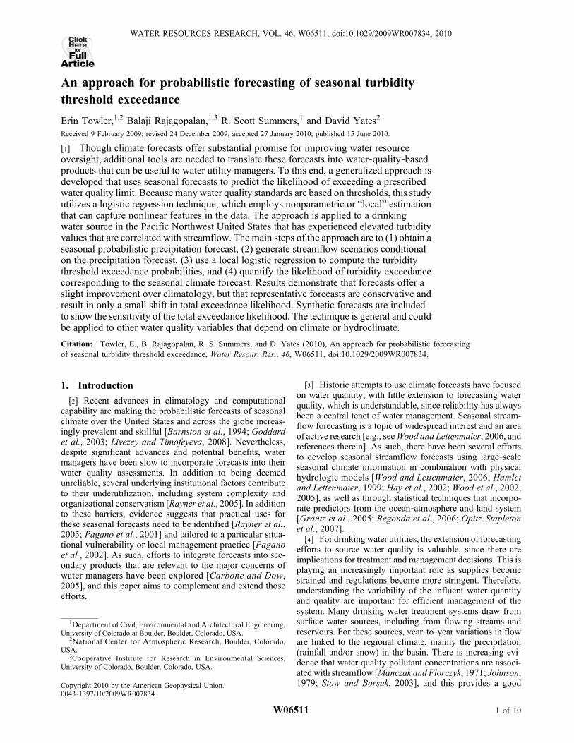
[13] The climate of the Pacific Northwest includes a dis-tinct wet winter season. The climate diagnostics in this sec-tion are shown as box plots, in which the box representsthe 25th and 75th percentile, the whiskers show the 5th and95th percentiles, points are values outside this range, and thehorizontal line represents the median. For the case studyregion, box plots of the average monthly precipitation(Figure 1) and average monthly streamflows (Figure 2) showthat the winter months (November–February) include gen-

Figure 1. Averagemonthly precipitation in the study regionfor January (J) through December (D).

TOWLER ET AL.: FORECAST TURBIDITY THRESH W06511W06511

2 of 10

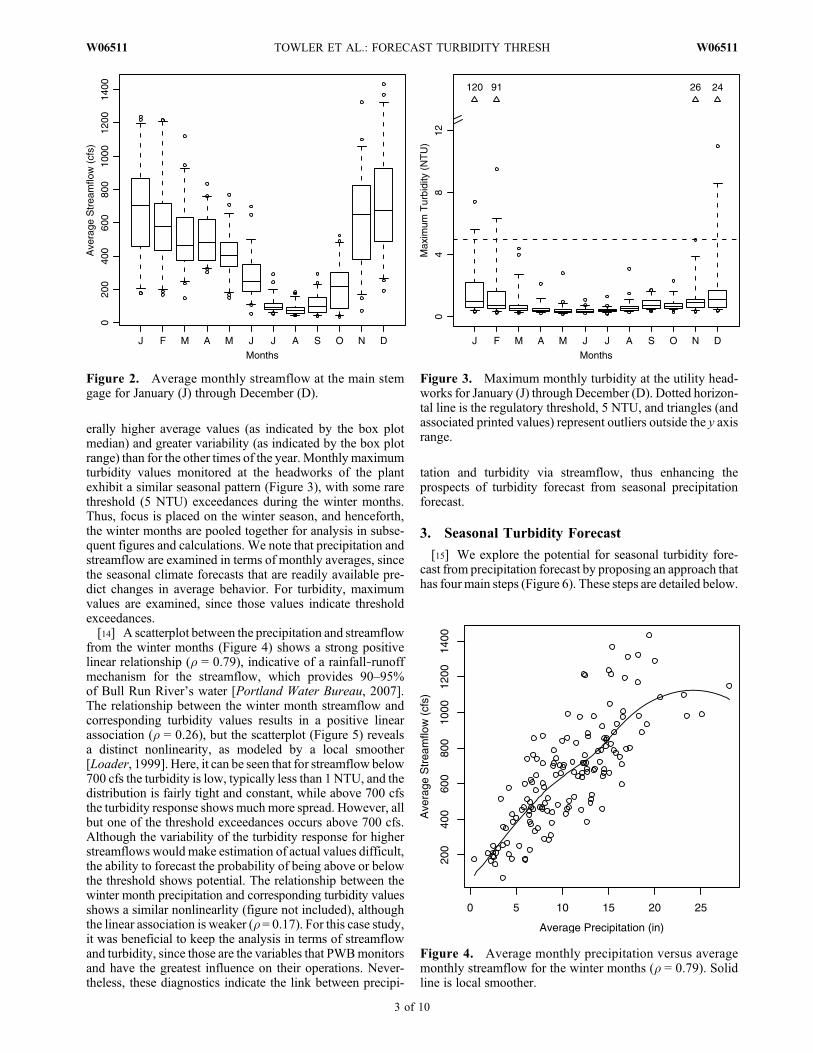
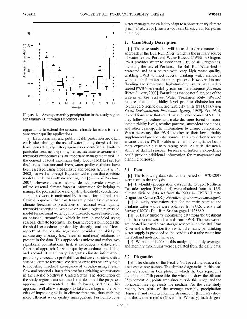
erally higher average values (as indicated by the box plotmedian) and greater variability (as indicated by the box plotrange) than for the other times of the year. Monthly maximumturbidity values monitored at the headworks of the plantexhibit a similar seasonal pattern (Figure 3), with some rarethreshold (5 NTU) exceedances during the winter months.Thus, focus is placed on the winter season, and henceforth,the winter months are pooled together for analysis in subse-quent figures and calculations. We note that precipitation andstreamflow are examined in terms of monthly averages, sincethe seasonal climate forecasts that are readily available pre-dict changes in average behavior. For turbidity, maximumvalues are examined, since those values indicate thresholdexceedances.[14] A scatterplot between the precipitation and streamflow

from the winter months (Figure 4) shows a strong positivelinear relationship (r = 0.79), indicative of a rainfall‐runoffmechanism for the streamflow, which provides 90–95%of Bull Run River’s water [Portland Water Bureau, 2007].The relationship between the winter month streamflow andcorresponding turbidity values results in a positive linearassociation (r = 0.26), but the scatterplot (Figure 5) revealsa distinct nonlinearity, as modeled by a local smoother[Loader, 1999]. Here, it can be seen that for streamflow below700 cfs the turbidity is low, typically less than 1 NTU, and thedistribution is fairly tight and constant, while above 700 cfsthe turbidity response showsmuchmore spread. However, allbut one of the threshold exceedances occurs above 700 cfs.Although the variability of the turbidity response for higherstreamflows would make estimation of actual values difficult,the ability to forecast the probability of being above or belowthe threshold shows potential. The relationship between thewinter month precipitation and corresponding turbidity valuesshows a similar nonlinearlity (figure not included), althoughthe linear association is weaker (r = 0.17). For this case study,it was beneficial to keep the analysis in terms of streamflowand turbidity, since those are the variables that PWBmonitorsand have the greatest influence on their operations. Never-theless, these diagnostics indicate the link between precipi-

tation and turbidity via streamflow, thus enhancing theprospects of turbidity forecast from seasonal precipitationforecast.

3. Seasonal Turbidity Forecast

[15] We explore the potential for seasonal turbidity fore-cast from precipitation forecast by proposing an approach thathas four main steps (Figure 6). These steps are detailed below.

Figure 2. Average monthly streamflow at the main stemgage for January (J) through December (D).

Figure 3. Maximum monthly turbidity at the utility head-works for January (J) through December (D). Dotted horizon-tal line is the regulatory threshold, 5 NTU, and triangles (andassociated printed values) represent outliers outside the y axisrange.

Figure 4. Average monthly precipitation versus averagemonthly streamflow for the winter months (r = 0.79). Solidline is local smoother.


3 of 10

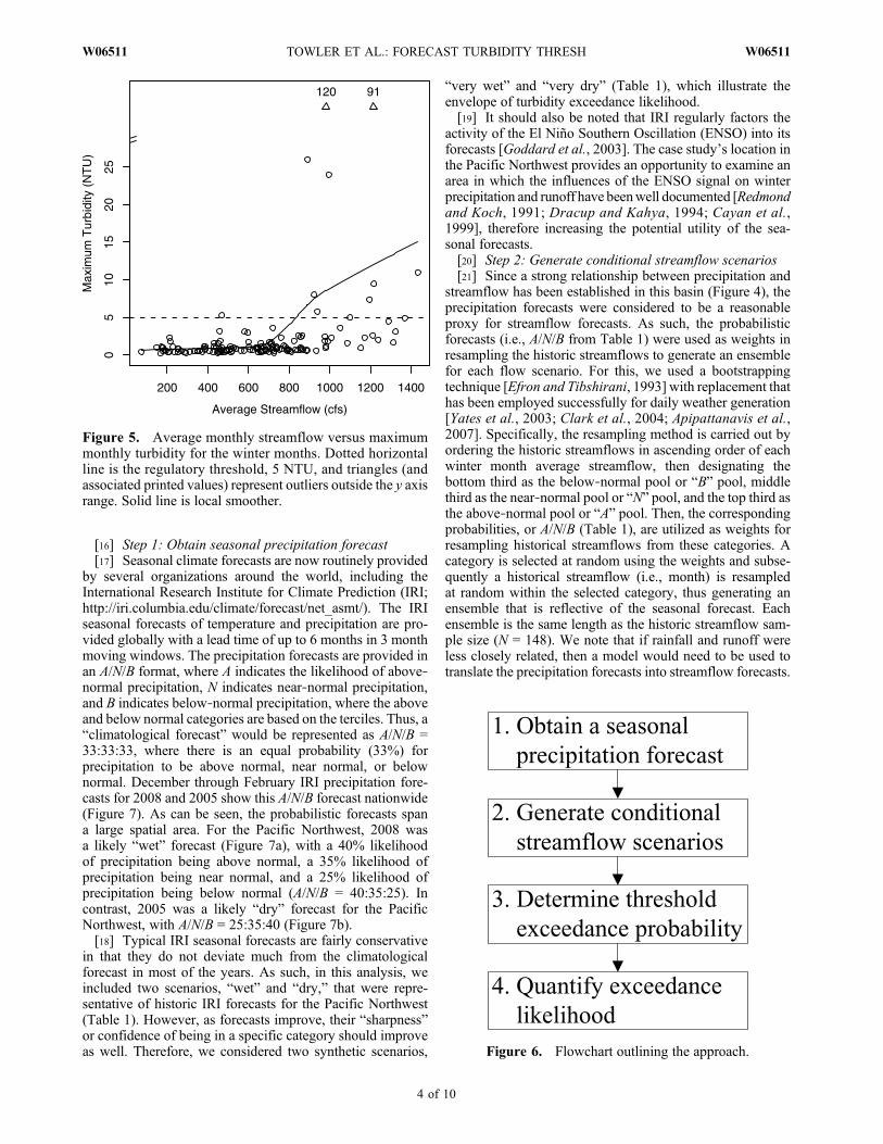
[16] Step 1: Obtain seasonal precipitation forecast[17] Seasonal climate forecasts are now routinely provided

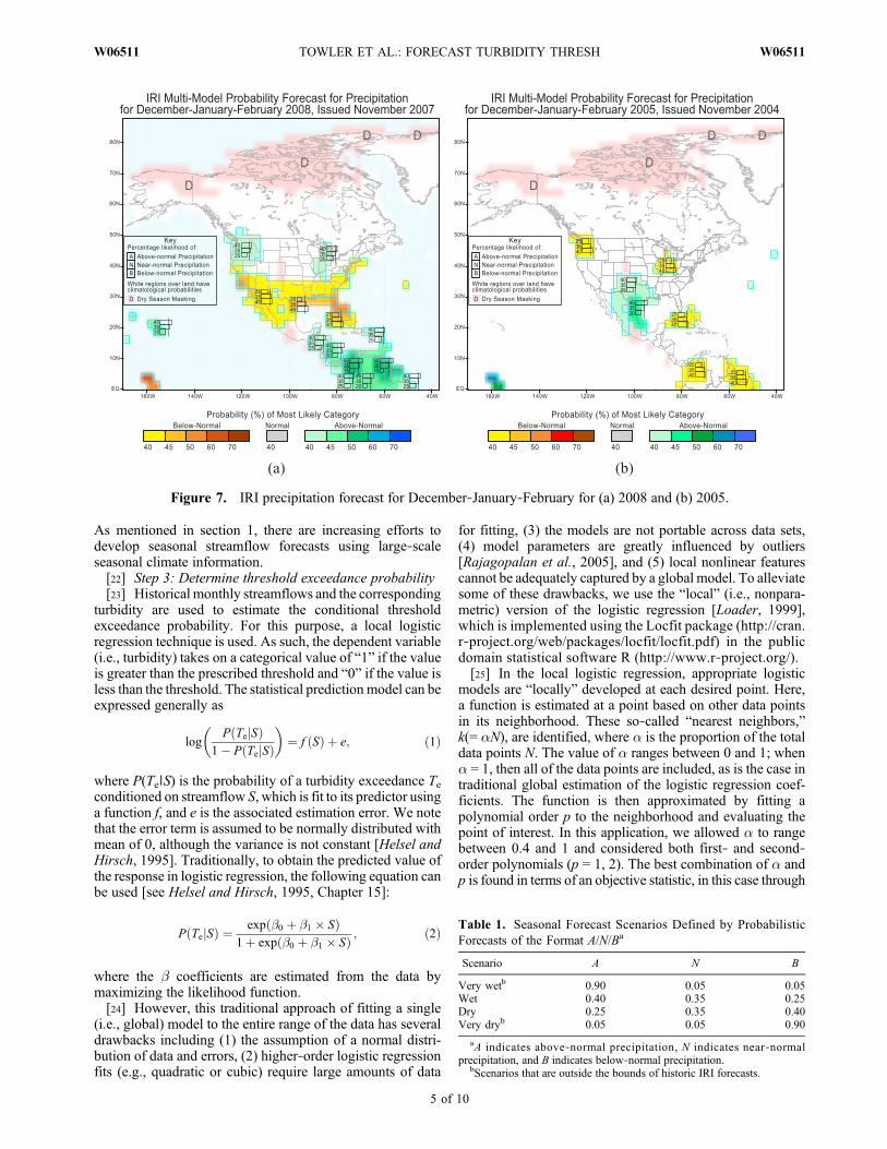
by several organizations around the world, including theInternational Research Institute for Climate Prediction (IRI;http://iri.columbia.edu/climate/forecast/net_asmt/). The IRIseasonal forecasts of temperature and precipitation are pro-vided globally with a lead time of up to 6 months in 3 monthmoving windows. The precipitation forecasts are provided inan A/N/B format, where A indicates the likelihood of above‐normal precipitation, N indicates near‐normal precipitation,and B indicates below‐normal precipitation, where the aboveand below normal categories are based on the terciles. Thus, a“climatological forecast” would be represented as A/N/B =33:33:33, where there is an equal probability (33%) forprecipitation to be above normal, near normal, or belownormal. December through February IRI precipitation fore-casts for 2008 and 2005 show this A/N/B forecast nationwide(Figure 7). As can be seen, the probabilistic forecasts spana large spatial area. For the Pacific Northwest, 2008 wasa likely “wet” forecast (Figure 7a), with a 40% likelihoodof precipitation being above normal, a 35% likelihood ofprecipitation being near normal, and a 25% likelihood ofprecipitation being below normal (A/N/B = 40:35:25). Incontrast, 2005 was a likely “dry” forecast for the PacificNorthwest, with A/N/B = 25:35:40 (Figure 7b).[18] Typical IRI seasonal forecasts are fairly conservative

in that they do not deviate much from the climatologicalforecast in most of the years. As such, in this analysis, weincluded two scenarios, “wet” and “dry,” that were repre-sentative of historic IRI forecasts for the Pacific Northwest(Table 1). However, as forecasts improve, their “sharpness”or confidence of being in a specific category should improveas well. Therefore, we considered two synthetic scenarios,

“very wet” and “very dry” (Table 1), which illustrate theenvelope of turbidity exceedance likelihood.[19] It should also be noted that IRI regularly factors the

activity of the El Niño Southern Oscillation (ENSO) into itsforecasts [Goddard et al., 2003]. The case study’s location inthe Pacific Northwest provides an opportunity to examine anarea in which the influences of the ENSO signal on winterprecipitation and runoff have beenwell documented [Redmondand Koch, 1991; Dracup and Kahya, 1994; Cayan et al.,1999], therefore increasing the potential utility of the sea-sonal forecasts.[20] Step 2: Generate conditional streamflow scenarios[21] Since a strong relationship between precipitation and

streamflow has been established in this basin (Figure 4), theprecipitation forecasts were considered to be a reasonableproxy for streamflow forecasts. As such, the probabilisticforecasts (i.e., A/N/B from Table 1) were used as weights inresampling the historic streamflows to generate an ensemblefor each flow scenario. For this, we used a bootstrappingtechnique [Efron and Tibshirani, 1993] with replacement thathas been employed successfully for daily weather generation[Yates et al., 2003; Clark et al., 2004; Apipattanavis et al.,2007]. Specifically, the resampling method is carried out byordering the historic streamflows in ascending order of eachwinter month average streamflow, then designating thebottom third as the below‐normal pool or “B” pool, middlethird as the near‐normal pool or “N” pool, and the top third asthe above‐normal pool or “A” pool. Then, the correspondingprobabilities, or A/N/B (Table 1), are utilized as weights forresampling historical streamflows from these categories. Acategory is selected at random using the weights and subse-quently a historical streamflow (i.e., month) is resampledat random within the selected category, thus generating anensemble that is reflective of the seasonal forecast. Eachensemble is the same length as the historic streamflow sam-ple size (N = 148). We note that if rainfall and runoff wereless closely related, then a model would need to be used totranslate the precipitation forecasts into streamflow forecasts.

Figure 5. Average monthly streamflow versus maximummonthly turbidity for the winter months. Dotted horizontalline is the regulatory threshold, 5 NTU, and triangles (andassociated printed values) represent outliers outside the y axisrange. Solid line is local smoother.

Figure 6. Flowchart outlining the approach.


4 of 10

As mentioned in section 1, there are increasing efforts todevelop seasonal streamflow forecasts using large‐scaleseasonal climate information.[22] Step 3: Determine threshold exceedance probability[23] Historical monthly streamflows and the corresponding

turbidity are used to estimate the conditional thresholdexceedance probability. For this purpose, a local logisticregression technique is used. As such, the dependent variable(i.e., turbidity) takes on a categorical value of “1” if the valueis greater than the prescribed threshold and “0” if the value isless than the threshold. The statistical prediction model can beexpressed generally as

logPðTejSÞ

1� PðTejSÞ� �

¼ f ðSÞ þ e; ð1Þ

where P(Te∣S) is the probability of a turbidity exceedance Teconditioned on streamflow S, which is fit to its predictor usinga function f, and e is the associated estimation error. We notethat the error term is assumed to be normally distributed withmean of 0, although the variance is not constant [Helsel andHirsch, 1995]. Traditionally, to obtain the predicted value ofthe response in logistic regression, the following equation canbe used [see Helsel and Hirsch, 1995, Chapter 15]:

PðTejSÞ ¼ expð�0 þ �1 � SÞ1þ expð�0 þ �1 � SÞ ; ð2Þ

where the b coefficients are estimated from the data bymaximizing the likelihood function.[24] However, this traditional approach of fitting a single

(i.e., global) model to the entire range of the data has severaldrawbacks including (1) the assumption of a normal distri-bution of data and errors, (2) higher‐order logistic regressionfits (e.g., quadratic or cubic) require large amounts of data

for fitting, (3) the models are not portable across data sets,(4) model parameters are greatly influenced by outliers[Rajagopalan et al., 2005], and (5) local nonlinear featurescannot be adequately captured by a global model. To alleviatesome of these drawbacks, we use the “local” (i.e., nonpara-metric) version of the logistic regression [Loader, 1999],which is implemented using the Locfit package (http://cran.r‐project.org/web/packages/locfit/locfit.pdf) in the publicdomain statistical software R (http://www.r‐project.org/).[25] In the local logistic regression, appropriate logistic

models are “locally” developed at each desired point. Here,a function is estimated at a point based on other data pointsin its neighborhood. These so‐called “nearest neighbors,”k(= aN), are identified, where a is the proportion of the totaldata points N. The value of a ranges between 0 and 1; whena = 1, then all of the data points are included, as is the case intraditional global estimation of the logistic regression coef-ficients. The function is then approximated by fitting apolynomial order p to the neighborhood and evaluating thepoint of interest. In this application, we allowed a to rangebetween 0.4 and 1 and considered both first‐ and second‐order polynomials (p = 1, 2). The best combination of a andp is found in terms of an objective statistic, in this case through

Figure 7. IRI precipitation forecast for December‐January‐February for (a) 2008 and (b) 2005.

Table 1. Seasonal Forecast Scenarios Defined by ProbabilisticForecasts of the Format A/N/Ba

Scenario A N B

Very wetb 0.90 0.05 0.05Wet 0.40 0.35 0.25Dry 0.25 0.35 0.40Very dryb 0.05 0.05 0.90

aA indicates above‐normal precipitation, N indicates near‐normalprecipitation, and B indicates below‐normal precipitation.

bScenarios that are outside the bounds of historic IRI forecasts.


5 of 10

minimization of the generalized cross‐validation (GCV) sta-tistic [Loader, 1999]. The GCV function is defined as

GCVð�; pÞ ¼PNi¼1

ðyi�yiÞ2N

1� mN

� �2 ; ð3Þ

where yi − yi is the residual (error) between the observed andpredicted values, N is the number of data points, and m is thedegrees of freedom of the fitted polynomial [Loader, 1999,p. 31]. The GCV has been found to be a good estimate ofthe predictive risk of a model, unlike other functions which aregoodness of fit measures [Craven and Wahba, 1979]. We notethat local logistic regression is more computationally intensivethan the global approach, but this is barely an issue with recentadvances in computing power.[26] To provide an estimate for the amount of uncertainty

explained by the logistic model, a likelihood R2 can be cal-culated as

R2 ¼ 1� L

L0; ð4Þ

where L is the log likelihood of the fit logistic model and L0 isthe log likelihood of the intercept‐only model. L is calculatedas [see Helsel and Hirsch, 1995, Chapter 15]

L ¼XNi¼1

½yi lnðpiÞ þ ð1� yiÞ lnð1� piÞ�; ð5Þ

where yi is the binary observations and pi is the predictedprobabilities for observations i = 1,N. L is a negative number,so the coefficients are estimated so as to maximize it (i.e.,bring it closer to 0).[27] In this application, the diagnostics indicated that the

water quality variable of interest T could be sufficientlydescribed by a single predictor variable S. However, whenusing this approach generally (i.e., at another location and/orfor another water quality variable), there may be multiplepredictors that need to be considered (e.g., streamflow andwater temperature). We note that, methodologically, it wouldbe straightforward to fit the logistic function to a suite of best‐fitting predictor variables, which could be found through anobjective criteria statistic, such as the aforementioned GCV.We emphasize the importance of data diagnostics in predictorselection and in determining the appropriateness of using thisapproach.[28] Step 4: Quantify exceedance likelihood[29] The key quantity of interest is the total likelihood of

water quality threshold exceedance for a given seasonalforecast. As such, the theorem of total probability [Ang andTang, 2007] can be modified into its continuous form toobtain

PðTeÞ ¼Z1

0

PðTejSf Þ�PðSf ÞdSf ; ð6Þ

where P(Te) is the likelihood of a turbidity exceedance giventhe seasonal forecast, P(Te∣Sf) is the conditional thresholdexceedance probability found in Step 3, and P(Sf) is thestreamflow density distribution under the forecast. The empir-

ical probability density function (PDF) from the streamflowensemble generated in Step 2 is used to quantify P(Sf).

4. Results

4.1. Turbidity Forecast Quantification

[30] Following the main steps of the approach, the likeli-hood estimates are computed for the four forecast scenarios(Table 1) along with the historical record, which provides aclimatological comparison.[31] For each of the forecast scenarios, the empirical dis-

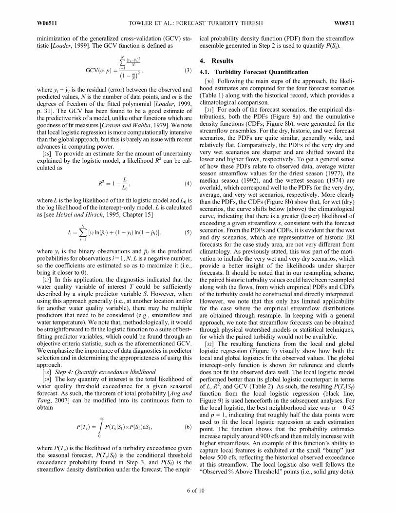
tributions, both the PDFs (Figure 8a) and the cumulativedensity functions (CDFs; Figure 8b), were generated for thestreamflow ensembles. For the dry, historic, and wet forecastscenarios, the PDFs are quite similar, generally wide, andrelatively flat. Comparatively, the PDFs of the very dry andvery wet scenarios are sharper and are shifted toward thelower and higher flows, respectively. To get a general senseof how these PDFs relate to observed data, average winterseason streamflow values for the driest season (1977), themedian season (1992), and the wettest season (1974) areoverlaid, which correspond well to the PDFs for the very dry,average, and very wet scenarios, respectively. More clearlythan the PDFs, the CDFs (Figure 8b) show that, for wet (dry)scenarios, the curve shifts below (above) the climatologicalcurve, indicating that there is a greater (lesser) likelihood ofexceeding a given streamflow s, consistent with the forecastscenarios. From the PDFs and CDFs, it is evident that the wetand dry scenarios, which are representative of historic IRIforecasts for the case study area, are not very different fromclimatology. As previously stated, this was part of the moti-vation to include the very wet and very dry scenarios, whichprovide a better insight of the likelihoods under sharperforecasts. It should be noted that in our resampling scheme,the paired historic turbidity values could have been resampledalong with the flows, from which empirical PDFs and CDFsof the turbidity could be constructed and directly interpreted.However, we note that this only has limited applicabilityfor the case where the empirical streamflow distributionsare obtained through resample. In keeping with a generalapproach, we note that streamflow forecasts can be obtainedthrough physical watershed models or statistical techniques,for which the paired turbidity would not be available.[32] The resulting functions from the local and global

logistic regression (Figure 9) visually show how both thelocal and global logistics fit the observed values. The globalintercept‐only function is shown for reference and clearlydoes not fit the observed data well. The local logistic modelperformed better than its global logistic counterpart in termsof L, R2, and GCV (Table 2). As such, the resulting P(Te∣Sf)function from the local logistic regression (black line,Figure 9) is used henceforth in the subsequent analyses. Forthe local logistic, the best neighborhood size was a = 0.45and p = 1, indicating that roughly half the data points wereused to fit the local logistic regression at each estimationpoint. The function shows that the probability estimatesincrease rapidly around 900 cfs and then mildly increase withhigher streamflows. An example of this function’s ability tocapture local features is exhibited at the small “bump” justbelow 500 cfs, reflecting the historical observed exceedanceat this streamflow. The local logistic also well follows the“Observed % Above Threshold” points (i.e., solid gray dots).


6 of 10

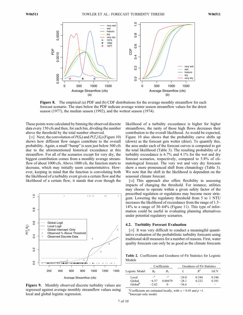
These points were calculated by binning the observed discretedata every 150 cfs and then, for each bin, dividing the numberabove the threshold by the total number observed.[33] Next, the convolution ofP(Sf) andP(Te∣Sf) (Figure 10)

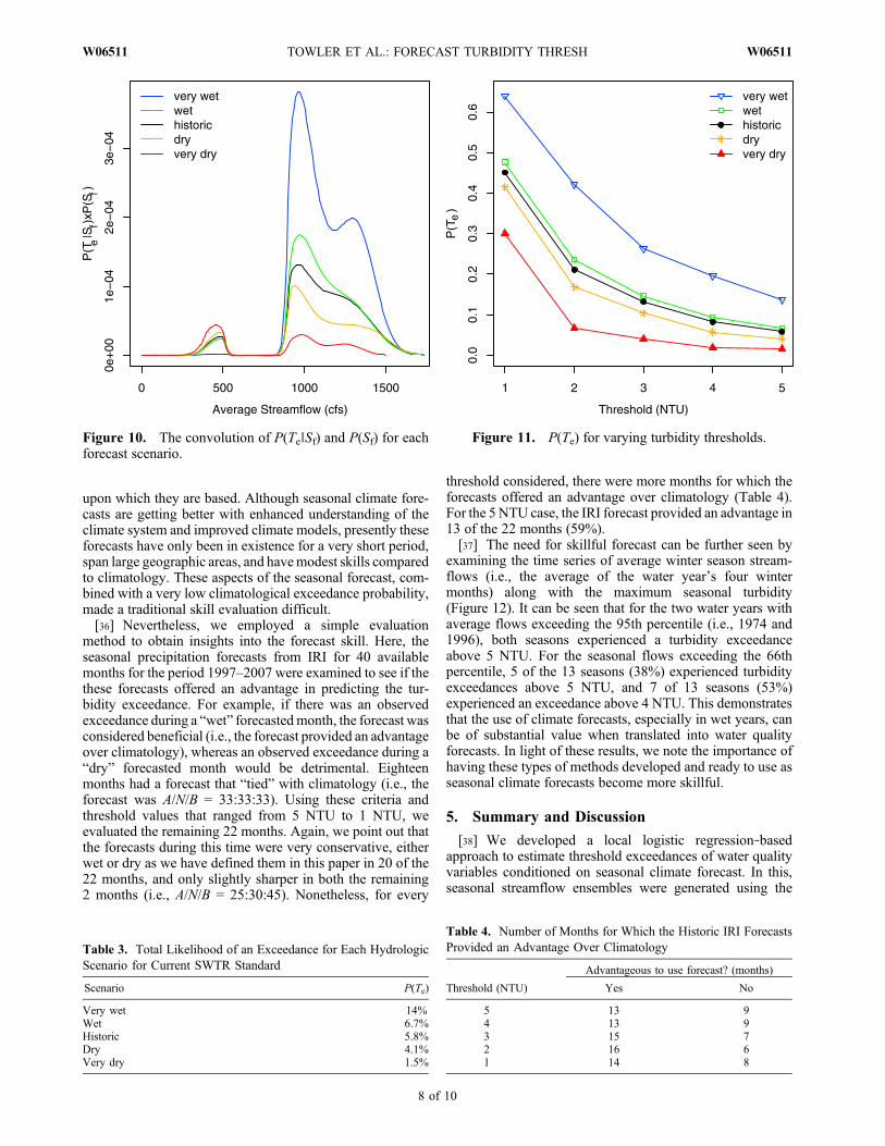
shows how different flow ranges contribute to the overallprobability. Again, a small “bump” is seen just below 500 cfsdue to the aforementioned historical exceedance at thisstreamflow. For all of the scenarios except for very dry, thebiggest contribution comes from a monthly average stream-flow of about 1000 cfs. Above 1000 cfs, the function starts todecrease, which may initially seem counterintuitive. How-ever, keeping in mind that the function is convoluting boththe likelihood of a turbidity event given a certain flow and thelikelihood of a certain flow, it stands that even though the

likelihood of a turbidity exceedance is higher for higherstreamflows, the rarity of those high flows decreases theircontribution to the overall likelihood. As would be expected,Figure 10 also shows that the probability curve shifts up(down) as the forecast gets wetter (drier). To quantify this,the area under each of the forecast curves is computed to getthe total likelihood (Table 3). The resulting probability of aturbidity exceedance is 6.7% and 4.1% for the wet and dryforecast scenarios, respectively, compared to 5.8% of cli-matological forecast. The very wet and very dry forecastsshow a more pronounced shift from climatology (Table 3).We note that the shift in the likelihood is dependent on theseasonal climate forecast.[34] This approach also offers flexibility in assessing

impacts of changing the threshold. For instance, utilitiesmay choose to operate within a given safety factor of theprescribed regulation or regulations may become more strin-gent. Lowering the regulatory threshold from 5 to 1 NTUincreases the likelihood of exceedance from the range of 1.5–14% to a range of 30–64% (Figure 11). This type of infor-mation could be useful in evaluating planning alternativesunder potential regulatory scenarios.

4.2. Turbidity Forecast Evaluation

[35] It was very difficult to conduct a meaningful quanti-tative evaluation of the probabilistic turbidity forecasts usingtraditional skill measures for a number of reasons. First, waterquality forecasts can only be as good as the climate forecasts

Figure 8. The empirical (a) PDF and (b) CDF distributions for the average monthly streamflow for eachforecast scenario. The stars below the PDF indicate average winter season streamflow values for the driestseason (1977), the median season (1992), and the wettest season (1974).

Figure 9. Monthly observed discrete turbidity values areregressed against average monthly streamflow values usinglocal and global logistic regression.

Table 2. Coefficients and Goodness‐of‐Fit Statistics for LogisticModels

Logistic Model

Coefficients Goodness‐of‐Fit Statistics

B0 B1 L R2 GCV

Local ‐a ‐a −24.0 0.344 0.346Global −6.57 0.00479 −28.1 0.232 0.391Globalb −2.62 0 −36.6 ‐ ‐

aCoefficients are estimated locally, with a = 0.45 and p =1.bIntercept‐only model.


7 of 10

upon which they are based. Although seasonal climate fore-casts are getting better with enhanced understanding of theclimate system and improved climate models, presently theseforecasts have only been in existence for a very short period,span large geographic areas, and havemodest skills comparedto climatology. These aspects of the seasonal forecast, com-bined with a very low climatological exceedance probability,made a traditional skill evaluation difficult.[36] Nevertheless, we employed a simple evaluation

method to obtain insights into the forecast skill. Here, theseasonal precipitation forecasts from IRI for 40 availablemonths for the period 1997–2007 were examined to see if thethese forecasts offered an advantage in predicting the tur-bidity exceedance. For example, if there was an observedexceedance during a “wet” forecastedmonth, the forecast wasconsidered beneficial (i.e., the forecast provided an advantageover climatology), whereas an observed exceedance during a“dry” forecasted month would be detrimental. Eighteenmonths had a forecast that “tied” with climatology (i.e., theforecast was A/N/B = 33:33:33). Using these criteria andthreshold values that ranged from 5 NTU to 1 NTU, weevaluated the remaining 22 months. Again, we point out thatthe forecasts during this time were very conservative, eitherwet or dry as we have defined them in this paper in 20 of the22 months, and only slightly sharper in both the remaining2 months (i.e., A/N/B = 25:30:45). Nonetheless, for every

threshold considered, there were more months for which theforecasts offered an advantage over climatology (Table 4).For the 5 NTU case, the IRI forecast provided an advantage in13 of the 22 months (59%).[37] The need for skillful forecast can be further seen by

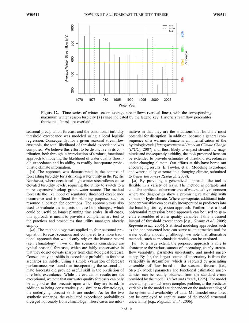
examining the time series of average winter season stream-flows (i.e., the average of the water year’s four wintermonths) along with the maximum seasonal turbidity(Figure 12). It can be seen that for the two water years withaverage flows exceeding the 95th percentile (i.e., 1974 and1996), both seasons experienced a turbidity exceedanceabove 5 NTU. For the seasonal flows exceeding the 66thpercentile, 5 of the 13 seasons (38%) experienced turbidityexceedances above 5 NTU, and 7 of 13 seasons (53%)experienced an exceedance above 4 NTU. This demonstratesthat the use of climate forecasts, especially in wet years, canbe of substantial value when translated into water qualityforecasts. In light of these results, we note the importance ofhaving these types of methods developed and ready to use asseasonal climate forecasts become more skillful.

5. Summary and Discussion

[38] We developed a local logistic regression‐basedapproach to estimate threshold exceedances of water qualityvariables conditioned on seasonal climate forecast. In this,seasonal streamflow ensembles were generated using the

Figure 10. The convolution of P(Te∣Sf) and P(Sf) for eachforecast scenario.

Table 3. Total Likelihood of an Exceedance for Each HydrologicScenario for Current SWTR Standard

Scenario P(Te)

Very wet 14%Wet 6.7%Historic 5.8%Dry 4.1%Very dry 1.5%

Figure 11. P(Te) for varying turbidity thresholds.

Table 4. Number of Months for Which the Historic IRI ForecastsProvided an Advantage Over Climatology

Threshold (NTU)

Advantageous to use forecast? (months)

Yes No

5 13 94 13 93 15 72 16 61 14 8


8 of 10

seasonal precipitation forecast and the conditional turbiditythreshold exceedance was modeled using a local logisticregression. Consequently, for a given seasonal streamflowensemble, the total likelihood of threshold exceedance wascomputed. We believe this effort to be distinctive in its con-tribution, both through its introduction of a robust, functionalapproach to modeling the likelihood of water quality thresh-old exceedance and its ability to readily incorporate proba-bilistic climate information.[39] The approach was demonstrated in the context of

forecasting turbidity for a drinking water utility in the PacificNorthwest, where occasional high winter streamflows causeelevated turbidity levels, requiring the utility to switch to amore expensive backup groundwater source. The methodforecasts the likelihood of regulatory threshold exceedanceoccurrence and is offered for planning purposes such asresource allocation for operations. The approach was alsoused to evaluate the impacts of threshold changes, whichcould be useful on longer planning time scales. In all cases,this approach is meant to provide a complementary tool tothe practices and procedures that utility managers alreadyemploy.[40] The methodology was applied to four seasonal pre-

cipitation forecast scenarios and compared to a more tradi-tional approach that would only rely on the historic record(i.e., climatology). Two of the scenarios considered aretypical seasonal forecasts, which are fairly conservative inthat they do not deviate sharply from climatological forecast.Consequently, the shifts in exceedance probabilities for thosescenarios are subtle. Using a simple evaluation of forecastperformance, we found that incorporating the seasonal cli-mate forecasts did provide useful skill in the prediction ofthreshold exceedance. While the evaluation results are notexceptional, we note that our water quality forecasts can onlybe as good as the forecasts upon which they are based. Inaddition to being conservative (i.e., similar to climatology),the underlying forecast skills are modest. As for the twosynthetic scenarios, the calculated exceedance probabilitiesdiverged noticeably from climatology. These cases are infor-

mative in that they are the situations that hold the mostpotential for disruption. In addition, because a general con-sequence of a warmer climate is an intensification of thehydrologic cycle [Intergovernmental Panel on Climate Change(IPCC), 2007] and, thus, likely to impact streamflow mag-nitude and consequently turbidity, the tools presented here canbe extended to provide estimates of threshold exceedancesunder changing climate. Our efforts at this have borne outencouraging results (E. Towler, et al., Modeling hydrologicand water quality extremes in a changing climate, submittedto Water Resources Research, 2009).[41] By providing a generalized approach, the tool is

flexible in a variety of ways. The method is portable andcould be applied to other measures of water quality of concernwhere the diagnostics show a promising relationship withclimate or hydroclimate. Where appropriate, additional inde-pendent variables can be easily incorporated as predictors intothe local logistic regression approach. Furthermore, a localpolynomial regression based approach can be used to gen-erate ensembles of water quality variables if this is desiredinstead of threshold exceedances [e.g., Grantz et al., 2005;Regonda et al., 2006]. Statistical modeling approaches suchas the one presented here can serve as an attractive tool forwater quality modeling, although we note that alternativemethods, such as mechanistic models, can be explored.[42] To a large extent, the proposed approach is able to

characterize the various sources of uncertainty, chiefly stream-flow variability, parameter uncertainty, and model uncer-tainty. By far, the largest source of uncertainty is from thevariability in streamflow, which is captured by generatingensembles of flow based on the seasonal forecast (i.e.,Step 2). Model parameter and functional estimation uncer-tainties can be readily obtained from the standard errorsprovided by the model [Helsel and Hirsch, 1995]. The modeluncertainty is a muchmore complex problem, as the predictorvariables in the model are dependent on the understanding ofthe system and availability of data. Multimodel ensemblescan be employed to capture some of the model structuraluncertainty [e.g., Regonda et al., 2006].

Figure 12. Time series of winter season average streamflows (vertical lines), with the correspondingmaximum winter season turbidity (T) range indicated by the legend key. Historic streamflow percentiles(horizontal lines) are overlaid.


9 of 10

[43] As regulations become more stringent and waterquality concerns become more prevalent, utility managerswill need additional tools to facilitate efficient planning andmanagement. As forecasts continue to improve, the ways inwhich they can contribute to water management should beexploited; the proposed approach provides an importantadvance in this endeavor.

[44] Acknowledgments. The authors would like to acknowledgeWater Research Foundation project 3132, “Incorporating climate changeinformation in water utility planning: A collaborative, decision analyticapproach,” the National Water Research Institute (NWRI) through a NWRIfellowship to the first author, and the U.S. EPA through a STAR fellowshipto the first author for partial financial support on this research effort. Thispublication was developed under a STAR Research Assistance AgreementF08C20433 awarded by the U.S. Environmental Protection Agency. It hasnot been formally reviewed by the EPA. The views expressed in this docu-ment are solely those of the authors, and the EPA does not endorse any pro-ducts or commercial services mentioned in this publication. The secondauthor is thankful to NCAR for providing a visitor fellowship during thecourse of this study. NCAR is sponsored by the National Science Founda-tion. In addition, they thank the staff of the Portland Water Bureau for pro-viding data and useful discussions.

ReferencesAng, A. H., and W. H. Tang (2007), Probability Concepts in Engineering:

Emphasis on Applications in Civil and Environmental Engineering,2nd ed., 406 pp., Wiley, New York.

Apipattanavis, S., G. Podesta, B. Rajagopalan, and R. W. Katz (2007),A semiparametric multivariate and multisite weather generator, WaterResour. Res., 43, W11401, doi:10.1029/2006WR005714.

Barnston, A. G., et al. (1994), Long‐lead seasonal forecasts— where do westand, Bull. Am. Meteorol. Soc., 75, 2097–2114.

Borsuk, M. E., C. A. Stow, and K. H. Reckhow (2002), Predicting the fre-quency of water quality standard violations: A probabilistic approach forTMDL development, Environ. Sci. Technol., 36, 2109–2115.

Carbone, G. J., and K. Dow (2005), Water resource management anddrought forecasts in South Carolina, J. Am. Water Resour. Assoc., 41,145–155.

Cayan, D. R., K. T. Redmond, and L. G. Riddle (1999), ENSO and hydro-logic extremes in the western United States, J. Clim., 12, 2881–2893.

Clark, M. P., S. Gangopadhyay, D. Brandon, K. Werner, L. Hay,B. Rajagopalan, and D. Yates (2004), A resampling procedure for gener-ating conditioned daily weather sequences, Water Resour. Res., 40,W04304, doi:10.1029/2003WR002747.

Craven, P., and G. Wahba (1979), Smoothing noisy data with splinefunctions — estimating the correct degree of smoothing by the methodof generalized cross‐validation, Numer. Math., 31, 377–403.

Dracup, J. A., and E. Kahya (1994), The relationships between UnitedStates streamflow and La Nina events, Water Resour. Res., 30(7),2133–2141, doi:10.1029/94WR00751.

Efron, B., and R. Tibshirani (1993), An Introduction to the Bootstrap,Monographs on Statistics and Applied Probability, vol. 57, 436 pp.,Chapman and Hall, New York.

Goddard, L., A. G. Barnston, and S. J. Mason (2003), Evaluation of theIRI’s “net assessment” seasonal climate forecasts 1997–2001, Bull.Am. Meteorol. Soc., 84, 1761–1781.

Grantz, K., B. Rajagopalan, M. Clark, and E. Zagona (2005), A techniquefor incorporating large‐scale climate information in basin‐scale ensemblestreamflow forecasts, Water Resour. Res., 41, W10410, doi:10.1029/2004WR003467.

Hamlet, A. F., and D. P. Lettenmaier (1999), Columbia River streamflowforecasting based on ENSO and PDO climate signals, J. Water Resour.Plann. Manage., 125, 333–341.

Hay, L. E., M. P. Clark, R. L. Wilby, W. J. Gutowski, G. H. Leavesley,Z. Pan, R.W. Arritt, and E. S. Takle (2002), Use of regional climate modeloutput for hydrologic simulations, J. Hydrometeorol., 3, 571–590.

Helsel, D. R., and R. M. Hirsch (1995), Studies in Environmental Science,in Statistical Methods in Water Resources, vol. 49, 529 pp., Elsevier,Amsterdam.

Intergovernmental Panel on Climate Change (IPCC) (2007), ClimateChange 2007: The Physical Science Basis : Contribution of WorkingGroup I to the Fourth Assessment Report of the Intergovernmental Panelon Climate Change, edited by S. Solomon, 996 pp., Cambridge Univer-sity Press, Cambridge.

Johnson, A. H. (1979), Estimating solute transport in streams fromgrab samples, Water Resour. Res., 15(5), 1224–1228, doi:10.1029/WR015i005p01224.

Livezey, R. E., and M. M. Timofeyeva (2008), The first decade of long‐lead US seasonal forecasts — insights from a skill analysis, Bull. Am.Meteorol. Soc., 89, 843–854.

Loader, C. (1999), Local Regression and Likelihood, Statistics and Com-puting, 290 pp., Springer, New York.

Manczak, H., and H. Florczyk (1971), Interpretation of results from thestudies of pollution of surface flowing waters, Water Res., 5, 575–584.

Milly, P. C. D., J. Betancourt, M. Falkenmark, R. M. Hirsch, Z. W.Kundzewicz, D. P. Lettenmaier, and R. J. Stouffer (2008), Climatechange — stationarity is dead: Whither water management?, Science,319, 573–574.

Opitz‐Stapleton, S., S. Gangopadhyay, and B. Rajagopalan (2007), Gener-ating streamflow forecasts for the Yakima River Basin using large‐scaleclimate predictors, J. Hydrol., 341, 131–143.

Pagano, T. C., H. C. Hartmann, and S. Sorooshian (2001), Using climateforecasts for water management: Arizona and the 1997–1998 El Nino,J. Am. Water Resour. Assoc., 37, 1139–1153.

Pagano, T. C., H. C. Hartmann, and S. Sorooshian (2002), Factors affectingseasonal forecast use in Arizona water management: A case study of the1997–98 El Nino, Clim. Res., 21, 259–269.

Portland Water Bureau (2007), Discover Your Drinking Water,2008(October 7), 5.

Qian, S. S., and K. H. Reckhow (2007), Combining model results andmonitoring data for water quality assessment, Environ. Sci. Technol.,41, 5008–5013.

Rajagopalan, B., K. Grantz, S. K. Regonda, M. Clark, and E. Zagona(2005), Ensemble streamflow forecasting: Methods and applications, inAdvances in Water Science Methodologies, edited by U. Aswathanarayana,Taylor and Francis, Netherlands.

Rayner, S., D. Lach, and H. Ingram (2005), Weather forecasts are forwimps: Why water resource managers do not use climate forecasts, Clim.Change, 69, 197–227.

Redmond, K. T., and R. W. Koch (1991), Surface climate and streamflowvariability in the western United States and their relationship to large‐scale circulation indexes, Water Resour. Res., 27(9), 2381–2399,doi:10.1029/91WR00690.

Regonda, S. K., B. Rajagopalan, M. Clark, and E. Zagona (2006), A multi-model ensemble forecast framework: Application to spring seasonalflows in the Gunnison River Basin, Water Resour. Res., 42, W09404,doi:10.1029/2005WR004653.

Stow, C. A., and M. E. Borsuk (2003), Assessing TMDL effectivenessusing flow‐adjusted concentrations: A case study of the Meuse River,North Carolina, Environ. Sci. Technol., 37, 2043–2050.

United States Environmental Protection Agency (1989), Final surface watertreatment rule, Federal Register 54:124:27486.

Wood, A. W., and D. P. Lettenmaier (2006), A test bed for new seasonalhydrologic forecasting approaches in the western United States, Bull.Am. Meteorol. Soc., 87, 1699–1712.

Wood, A. W., E. P. Maurer, A. Kumar, and D. P. Lettenmaier (2002),Long‐range experimental hydrologic forecasting for the eastern UnitedStates, J. Geophys. Res., 107(C10), 3170, doi:10.1029/2001JC001094.

Wood, A. W., A. Kumar, and D. P. Lettenmaier (2005), A retrospectiveassessment of National Centers for Environmental Prediction climatemodel‐based ensemble hydrologic forecasting in the western UnitedStates, J. Geophys. Res., 110, D04105, doi:10.1029/2004JD004508.

Yates, D., S. Gangopadhyay, B. Rajagopalan, and K. Strzepek (2003), Atechnique for generating regional climate scenarios using a nearest‐neighbor algorithm, Water Resour. Res., 39(7), 1199, doi:10.1029/2002WR001769.

B. Rajagopalan, R. S. Summers, and E. Towler, Department of Civil,Environmental and Architectural Engineering, University of Colorado atBoulder, 428 UCB, Boulder, CO 80309, USA. ([email protected])D. Yates, National Center for Atmospheric Research, P.O. Box 3000,

Boulder, CO 80309, USA.


10 of 10

An approach for probabilistic forecasting of seasonal turbidity threshold exceedance

Documents