An Applied Analysis of High-Dimensional Logistic Regressionsummit.sfu.ca/system/files/iritems1/17392/etd10164_DQiu.pdf · An Applied Analysis of High-Dimensional Logistic Regression

An Applied Analysis of High-DimensionalLogistic Regression

by

Derek Qiu

B.A., University of British Columbia, 2015

Project Submitted in Partial Fulfillment of the

Requirements for the Degree of

Master of Science

in the

Department of Statistics and Actuarial Science

Faculty of Science

c© Derek Qiu 2017SIMON FRASER UNIVERSITY

Summer 2017

All rights reserved.However, in accordance with the Copyright Act of Canada, this work may be reproduced

without authorization under the conditions for “Fair Dealing.” Therefore, limitedreproduction of this work for the purposes of private study, research, education, satire,parody, criticism, review and news reporting is likely to be in accordance with the law,

particularly if cited appropriately.

Approval

Name: Derek Qiu

Degree: Master of Science (Statistics)

Title: An Applied Analysis of High-Dimensional Logistic Regression

Examining Committee: Chair: Tim SwartzProfessor

Richard LockhartSenior SupervisorProfessor

Dave CampbellSupervisorAssociate Professor

Jiguo CaoInternal ExaminerAssociate Professor

Date Defended:

ii

Abstract

In the high dimensional setting, we investigate common regularization approaches for fitting logistic

regression models with binary response variables. A literature review is provided on generalized

linear models, regularization approaches which include the lasso, ridge, elastic net and relaxed

lasso, and recent post-selection methods for obtaining p-values of coefficient estimates proposed

by Lockhart et. al. and Buhlmann et. al. We consider varying n, p conditions, and assess model

performance based on several evaluation metrics - such as their sparsity, accuracy and algorithmic

time efficiency. Through a simulation study, we find that Buhlmann et. al’s multi sample splitting

method performed poorly when selected covariates were highly correlated. When λ was chosen

through cross validation, the elastic net had similar levels of performance as compared to the lasso,

but it did not possess the level of sparsity Zou and Hastie have suggested.

Keywords: High dimensional, logistic regression, lasso, elastic net, significance test

iii

Dedication

I dedicate this to everyone who has supported me on my journey thus far.

iv

Acknowledgements

I would like to begin by thanking my supervisor Dr. Richard Lockhart, for all the support, time and

effort he has put into helping me see this thesis through to completion. I would like to thank my

committee members for taking the time out of their busy schedules to participate in my defense. I

would like to thank my parents and siblings for their unwavering support and help throughout the

years. Finally, I would like to thank all the faculty, staff and students in our department for making

my time here at SFU such a wonderful experience.

v

Table of Contents

Approval ii

Abstract iii

Dedication iv

Acknowledgements v

Table of Contents vi

List of Tables viii

List of Figures xiii

1 Introduction 1

2 Literature Review 42.1 Generalized Linear Models . . . . . . . . . . . . . . . . . . . . . . . . . . . . . . 4

2.2 Regularization Approaches . . . . . . . . . . . . . . . . . . . . . . . . . . . . . . 9

2.2.1 Lasso . . . . . . . . . . . . . . . . . . . . . . . . . . . . . . . . . . . . . 9

2.2.2 Ridge Regression . . . . . . . . . . . . . . . . . . . . . . . . . . . . . . . 11

2.2.3 Elastic Net . . . . . . . . . . . . . . . . . . . . . . . . . . . . . . . . . . 13

2.2.4 Relaxed Lasso . . . . . . . . . . . . . . . . . . . . . . . . . . . . . . . . 13

2.3 Post Selection Inference . . . . . . . . . . . . . . . . . . . . . . . . . . . . . . . . 14

2.3.1 Covariance Test . . . . . . . . . . . . . . . . . . . . . . . . . . . . . . . . 14

2.3.2 p-value Estimation from multi-sample splitting . . . . . . . . . . . . . . . 15

3 Applied analysis of regularization approaches under varying n, p conditions. 163.1 Datasets . . . . . . . . . . . . . . . . . . . . . . . . . . . . . . . . . . . . . . . . 17

3.1.1 Birth Weight . . . . . . . . . . . . . . . . . . . . . . . . . . . . . . . . . 17

3.1.2 Riboflavin . . . . . . . . . . . . . . . . . . . . . . . . . . . . . . . . . . . 17

3.1.3 Test and Training Splits . . . . . . . . . . . . . . . . . . . . . . . . . . . . 17

3.2 Setup . . . . . . . . . . . . . . . . . . . . . . . . . . . . . . . . . . . . . . . . . 18

3.2.1 Choosing the Tuning Parameter . . . . . . . . . . . . . . . . . . . . . . . 18

vi

3.2.2 Case where n > p . . . . . . . . . . . . . . . . . . . . . . . . . . . . . . 18

3.2.3 Case where p > n . . . . . . . . . . . . . . . . . . . . . . . . . . . . . . 19

3.2.4 Case where n = p . . . . . . . . . . . . . . . . . . . . . . . . . . . . . . 19

3.3 Variable Selection . . . . . . . . . . . . . . . . . . . . . . . . . . . . . . . . . . . 19

3.3.1 Covariance Test . . . . . . . . . . . . . . . . . . . . . . . . . . . . . . . . 20

3.4 Model Evaluation . . . . . . . . . . . . . . . . . . . . . . . . . . . . . . . . . . . 21

3.4.1 Prediction Accuracy . . . . . . . . . . . . . . . . . . . . . . . . . . . . . 21

3.4.2 Logarithmic Loss . . . . . . . . . . . . . . . . . . . . . . . . . . . . . . . 22

3.4.3 Receiver Operating Characteristic Curves . . . . . . . . . . . . . . . . . . 23

4 Simulation Study 274.1 Simulation Design . . . . . . . . . . . . . . . . . . . . . . . . . . . . . . . . . . 27

4.2 Case where p > n . . . . . . . . . . . . . . . . . . . . . . . . . . . . . . . . . . . 29

4.2.1 Variable Selection . . . . . . . . . . . . . . . . . . . . . . . . . . . . . . 31

4.2.2 Model Evaluation . . . . . . . . . . . . . . . . . . . . . . . . . . . . . . . 37

4.3 Case where p = n, with highly correlated covariates. . . . . . . . . . . . . . . . . 40



4.4 Case where p = n, with randomly selected covariates. . . . . . . . . . . . . . . . . 46



4.5 Discussion of Results . . . . . . . . . . . . . . . . . . . . . . . . . . . . . . . . . 51

4.5.1 Evaluation Metrics . . . . . . . . . . . . . . . . . . . . . . . . . . . . . . 51

4.5.2 Sparsity . . . . . . . . . . . . . . . . . . . . . . . . . . . . . . . . . . . . 52

4.5.3 Multi Sample-Splitting . . . . . . . . . . . . . . . . . . . . . . . . . . . . 53

4.5.4 Covariance Test . . . . . . . . . . . . . . . . . . . . . . . . . . . . . . . . 55

4.5.5 Algorithm Runtime . . . . . . . . . . . . . . . . . . . . . . . . . . . . . . 56

4.5.6 How much are we losing from dichotomizing? . . . . . . . . . . . . . . . 57

4.5.7 Statistical Significance vs. Practical Significance . . . . . . . . . . . . . . 59

5 Conclusion 615.1 Extensions and Future Work . . . . . . . . . . . . . . . . . . . . . . . . . . . . . 61

Bibliography 63

Appendix A Code 65

Appendix B List of randomly selected covariates used in Case 3. 71

vii

List of Tables

Table 3.1 The estimated coefficients of the first 5 covariates to enter the Lasso and

elastic net fits are shown. The covariate# represents the column position of

the covariate in the design matrixX . . . . . . . . . . . . . . . . . . . . . 20

Table 3.2 The p-value and drop in covariance are shown for the first 5 covariates se-

lected using the Lasso in the case where p > n. . . . . . . . . . . . . . . . . 20

Table 3.3 The p-value and drop in covariance are shown for the first 5 covariates se-

lected using the Lasso in the case where p > n. . . . . . . . . . . . . . . . . 21

Table 3.4 Prediction accuracies for each of the four different regularization approaches

under the three varying n, p conditions. The birth weight dataset was used in

the case of n > p, while the riboflavin dataset was used for the case where

p > n. The final case of n = p made use of a subset of the riboflavin dataset. 22

Table 3.5 Logarithmic loss scores are shown for each of the four different fitting ap-

proaches under the three different n, p conditions. . . . . . . . . . . . . . . 22

Table 4.1 Coefficient estimates from fitting the standard linear model using only the

first 2 covariates selected by the Lasso. The response vector Y was centered,

while the design matrixX was centered and standardized. . . . . . . . . . 29

Table 4.2 Value of λ used to fit the preliminary Lasso to get coefficient estimates for

the simulation, and value of σ used for simulating our response vector. . . . 29

Table 4.3 The 5 covariates selected most frequently by the Lasso and elastic net with

10-fold cross validation across B = 100 samples. For each coefficient, the

number of times that variable was selected is given along with the mean and

average of the (non-zero) values. The covariate number represents the col-

umn position of the covariate in the design matrix. . . . . . . . . . . . . . . 31

Table 4.4 The number of times in 100 Monte Carlo samples that covariates 1278 and

4003 were selected by the Lasso, as well as the number of instances where

they are determined to be statistically significant. Proportions with respect to

the total are provided in parentheses. . . . . . . . . . . . . . . . . . . . . . 33

viii

Table 4.5 The number of times in 100 Monte Carlo samples that covariates 1278 and

4003 were determined to be significant, as well as the total number of in-

stances where they were the first, second, or third or later variable to be se-

lected by the Lasso, respectively. Proportions with respect to the total are

shown in parentheses. . . . . . . . . . . . . . . . . . . . . . . . . . . . . . 33

Table 4.6 The number of times in 100 Monte Carlo samples that a particular coefficient

was observed to enter the Lasso regularized model as the second and third

non-zero coefficient, when covariate 1278 enters the model first, ordered

by decreasing frequency. . . . . . . . . . . . . . . . . . . . . . . . . . . . 34

Table 4.7 The number of times in 100 Monte Carlo samples that a particular coefficient

was observed to enter the Lasso regularized model as the second and third

non-zero coefficient, when covariate 4003 enters the model first, ordered

by decreasing frequency. . . . . . . . . . . . . . . . . . . . . . . . . . . . 34

Table 4.8 The total number of times where covariates 1278 and 4003 were selected by

the elastic net, as well as the number of instances where they were deter-

mined to be statistically significant. Proportions with respect to the total are

provided in parentheses. . . . . . . . . . . . . . . . . . . . . . . . . . . . . 36

Table 4.9 Average prediction accuracies and standard deviations for each of the four

penalized regression methods investigated during the simulation. Evaluation

is done on the test set, using the model obtained from the training set. A total

of B = 100 iterations are run. . . . . . . . . . . . . . . . . . . . . . . . . . 37

Table 4.10 p-values with Bonferroni correction from paired comparison t-tests between

prediction accuracies obtained from the different penalized regression meth-

ods. None are determined to be significantly different from each other at the

α = 0.05 significance level. . . . . . . . . . . . . . . . . . . . . . . . . . . 37

Table 4.11 The average and standard deviation of the logarithmic loss scores, across

B = 100 Monte Carlo samples, for each of the different fitting approaches. . 38


log loss scores obtain from the different penalized regression methods. . . . 38

Table 4.13 The average and standard deviation of the AUC scores observed across B =100 Monte Carlo samples for each of the different fitting approaches. . . . . 39

Table 4.14 p-values with Bonferroni correction, are provided from paired comparison

t-tests between the different penalized regression methods. . . . . . . . . . . 39

Table 4.15 The 5 covariates selected most frequently by the Lasso with 10-fold cross

validation across B = 500 samples. For each coefficient, the number of

times that variable was selected is given along with the mean and average of

the (non-zero) values. . . . . . . . . . . . . . . . . . . . . . . . . . . . . . 40

ix

Table 4.16 The 5 covariates selected most frequently by the elastic net with 10-fold cross




Table 4.17 The number of times that covariates 1278 and 4003 were selected by the

Lasso, as well as the number of instances where they are found to be sig-

nificant using the covariance test. Proportions with respect to the total are

provided in parentheses. . . . . . . . . . . . . . . . . . . . . . . . . . . . . 41

Table 4.18 The number of times that covariates 1278 and 4003 are found to be signifi-

cant, as well as the number of times that they were the first, second, or third

or later variable to be selected by the Lasso, respectively. Proportions with

respect to the total are shown in parentheses. . . . . . . . . . . . . . . . . . 42

Table 4.19 Average prediction accuracies and standard deviations are provided for each

of the penalized regression methods. . . . . . . . . . . . . . . . . . . . . . 43

Table 4.20 p-values with Bonferroni correction, are provided from paired comparison

t-tests between the different fitting approaches. . . . . . . . . . . . . . . . . 43

Table 4.21 Average log loss scores and standard deviations are provided for each of the

penalized regression methods. . . . . . . . . . . . . . . . . . . . . . . . . . 44


log loss scores. . . . . . . . . . . . . . . . . . . . . . . . . . . . . . . . . 44

Table 4.23 Average AUC and standard deviations are provided for each of the classifica-

tion methods. . . . . . . . . . . . . . . . . . . . . . . . . . . . . . . . . . . 45


AUC scores. . . . . . . . . . . . . . . . . . . . . . . . . . . . . . . . . . . 45

Table 4.25 Coefficient estimates from fitting the standard linear model using only the

first two covariates (980 & 1287) selected by the Lasso in the p = n case

with randomly selected covariates. . . . . . . . . . . . . . . . . . . . . . . 46

Table 4.26 Value of λ used to fit the preliminary Lasso to get coefficient estimates for

the simulation, and value of σ used for simulating our response vector. . . . 46

Table 4.27 The 5 covariates selected most frequently by the Lasso with 10-fold cross



the (non-zero) values. The covariate number represents the column position

of the covariate in the original design matrixX . . . . . . . . . . . . . . . . 47

Table 4.28 The 5 covariates selected most frequently by the elastic net with 10-fold cross




x

Table 4.29 The average and standard deviation of the prediction accuracies obtained

from the penalized regression methods investigated during the simulation

for B = 500 Monte Carlo samples using 50 randomly selected covariate

columns. . . . . . . . . . . . . . . . . . . . . . . . . . . . . . . . . . . . . 48

Table 4.30 The average and standard deviation of the AUC scores obtained from the

penalized regression methods investigated during the simulation forB = 500Monte Carlo samples using 50 randomly selected covariate columns. . . . . 48

Table 4.31 The average and standard deviation of the log loss scores obtained from the

penalized regression methods investigated during the simulation forB = 500Monte Carlo samples using 50 randomly selected covariate columns. . . . . 49

Table 4.32 p-values with Bonferroni correction, are provided from multiple t-tests be-

tween the prediction accuracies obtained from the different penalized regres-

sion methods. . . . . . . . . . . . . . . . . . . . . . . . . . . . . . . . . . 49


tween the AUC scores obtained from the different penalized regression meth-

ods. . . . . . . . . . . . . . . . . . . . . . . . . . . . . . . . . . . . . . . 49


tween the log loss scores obtained from the different penalized regression

methods. . . . . . . . . . . . . . . . . . . . . . . . . . . . . . . . . . . . . 50

Table 4.35 Summary of results obtained from each of the 3 different cases investigated

during the simulation. In Case 1., we had p > n, Case 2. p = n with the 50

highest correlated covariates, and in Case 3. we had p = n with 50 randomly

chosen covariates. . . . . . . . . . . . . . . . . . . . . . . . . . . . . . . . 51

Table 4.36 The number of covariates selected by the Lasso and elastic net regularizations

under the three different n, p conditions. . . . . . . . . . . . . . . . . . . . 52

Table 4.37 Algorithm runtimes (seconds) are provided for each of the different fitting

approaches employed under different n, p conditions. . . . . . . . . . . . . 56

Table 4.38 Average runtimes (seconds) are provided for each of the different approaches

employed under different n, p conditions for obtaining p-values for Lasso

coefficient estimates. . . . . . . . . . . . . . . . . . . . . . . . . . . . . . 57

Table 4.39 Pre- and post-dichotomized average prediction accuracies and standard de-

viations in the case where p > n for each of the four classification methods

investigated during the simulation. A total of B = 100 Monte Carlo sam-

ples are run. The p-values are from a two-sided paired comparison t-test of

the hypothesis that there is no difference between the classification methods.

Significance at α levels of 0.05, 0.01, 0.001 is denoted by the varying num-

ber of asterisks (∗). . . . . . . . . . . . . . . . . . . . . . . . . . . . . . . . 58

xi

Table 4.40 Pre- and post-dichotomized average prediction accuracies and standard devi-

ations in the case where p = n with highly correlated covariates, for each of

the four classification methods investigated during the simulation. A total of

B = 500 Monte Carlo samples are run. . . . . . . . . . . . . . . . . . . . 59

Table 4.41 Pre- and post-dichotomized average prediction accuracies and standard devi-

ations in the case where p = n with randomly selected covariates, for each

of the four classification methods investigated during the simulation. A total

of B = 500 Monte Carlo samples are run. . . . . . . . . . . . . . . . . . . 59

xii

List of Figures

Figure 3.1 Receiver operating characteristic (ROC) curves are shown for each of the

following: (a) logistic regression with Lasso penalty, (b) logistic regres-

sion with ridge penalty, (c) logistic regression with elastic net penalty, and

(d) the relaxed Lasso, in the case where n > p using the birth weight

dataset. The ROC curve shows the tradeoff between the true positive rate

and false positive rate for a binary classifier, and in particular, the perfect

classifier would have a ROC curve that extends vertically from 0 to 1 and

horizontally across from 0 to 1 as well, hence maximizing the area under

the curve. . . . . . . . . . . . . . . . . . . . . . . . . . . . . . . . . . . 24


following: (a) logistic regression with Lasso penalty, (b) logistic regression

with ridge penalty, (c) logistic regression with elastic net penalty, and (d)

the relaxed Lasso, in the case where p > n using the riboflavin dataset. . . 25


following: (a) logistic regression with Lasso penalty, (b) logistic regression

with ridge penalty, (c) logistic regression with elastic net penalty, and (d)

the relaxed Lasso, in the case where p = n using a subset of the riboflavin

dataset. . . . . . . . . . . . . . . . . . . . . . . . . . . . . . . . . . . . 26

Figure 4.1 A correlation plot is shown for the five covariates that have the highest

correlation with the response variable, in descending order. Among the

five, covariates 1278 and 4003 are the first two to be selected by the Lasso. 30

Figure 4.2 The correlation structure between covariates 1278, 4003, the ones identi-

fied in Table 4.6 & Table 4.7, and the centered response vector Y in the

original riboflavin dataset. . . . . . . . . . . . . . . . . . . . . . . . . . 35

Figure 4.3 The covariance structure between covariates 1278, 1279, 4003 and the re-

sponse vector y are shown. Darker colors represent stronger correlations. . 54

Figure 4.4 The covariance test statistics T1 and T2 for the first and second coefficients

to enter the model along the Lasso solution path, across the B = 100iterations of the simulation, are plotted against each other. . . . . . . . . . 56

xiii

Chapter 1

Introduction

In the present day and age, the amount of data consistently being created is increasing at an

alarming rate [11]. With such large volumes of data, the demand for tools that are capable of

extracting usable and useful information is steadily rising. In particular, predictive models that are

capable of providing accurate and precise results that enable data-driven decision making are of vital

importance. In this paper, we place our main focus on a logistic regression model targeted at binary

classification - and in particular, its properties, applications and performance in a high-dimensional

setting.

Logistic regression models are a class of generalized linear models that are commonly applied

when we wish to estimate the relationship between a categorical response variable and one or more

covariates. In the simple case, which will be the focus for the remainder of this paper, the response

variable is dichotomous (i.e. only takes on two possible values). Suppose that we have independent

responses yi, where yi ∈ {0, 1}, and corresponding covariates xi = (xi1, xi2, ... xip), i = 1, 2, ... n.

Let α be the intercept and βj , j = 1, 2, ... p, be the coefficients to be estimated. Denote by πi the

probability of our response variable observing a success (i.e. takes the value 1) given the observed

data − that is to say, let πi = P(Yi = 1 | xi). The logistic regression model then takes the form:

log(

πi1− πi

)= α+

p∑j=1

xijβj (1.1)

As such, it can be seen that we are directly modeling the log odds that our response variable

observes a success, where we define odds as the ratio of the probability of observing a success to that

of a failure - that is to say, how much more likely we are to observe a success occuring as opposed to

a failure. For instance, if we have that π = 0.7, the odds of success would be 0.70.3 = 2.1, which tells

us that we are 2.1 times as likely to observe a success as a failure. In the insurance business, logistic

regression is commonly utilized as one of the possible ways of detecting fraudulent claims [20].

Suppose that we have a dataset with n = 100 sample observations of 3 variables - the fraudulent

status, age and gender of a particular claimant. Let the fraudulent status of a given claim be our

1

response variable, and assume that it takes only 2 possible values (’Yes’ and ’No’). We let age

and gender be our covariates. To construct a logistic regression model, we then would regress our

response on our 2 covariates, in order to build a relationship that enables us to predict the probability

of observing fraudulent behavior for a particular claim.

In the simple case described, we had n = 100 sample observations and p = 2 predictors.

However, it is now often the case in practice that datasets have several hundreds of predictors,

and we would like to identify a small subset of the truly important ones to be incorporated in the

final model. This is due to the fact that sparser models are more desirable, since they are faster to

implement, more memory-efficient to store, and easier to interpret. When the number of predictors

p gets very large, we are placed in the high-dimensional regression setting, and this creates problems

if we attempt to build models under traditional assumptions.

Traditionally, when constructing predictive models, it was usually the case that we have n > p.

That is to say, the number n of observations in our dataset, exceeds the number of predictors p that

we have. This relation, n > p, has to be satisfied in order to obtain ordinary least squares estimates

for our predictors in a standard linear regression setting. However, there also exist scenarios where

we have p > n, where the number of predictors is larger than the number of sample observations

that we have. This is commonly observed in the field of genomics when working with gene expres-

sion data, where the number of samples tends to be much smaller than the number of genes that

are measured, and this poses as a problem when we attempt to obtain regression estimates using

traditional methods.

To illustrate some of these issues, we begin by considering the standard linear regression model

in the case where we have n > p. Here, X ∈ Rn×p is our design matrix, where the ith row of

X is xi = (xi1, xi2, . . . xip), and the jth column of X is xj = (x1j , x2j , . . . xnj)T . Let Y

be a vector of n response variables and ε be a vector of independently and identically distributed

N(0, σ2) variates. We then have the usual linear model:

Y = Xβ + ε (1.2)

Now, in order to obtain estimates for β, the most common course of action is to minimize the

residual sum of squares, as shown below:

β = arg minβ∈Rp

||Y −Xβ||22 (1.3)

Subsequently, solving yields the closed-form ordinary least squares estimate for β.

β = (XTX)−1XTY (1.4)

One might notice that in order for this closed form solution to exist and be well-defined, the columns

of X have to be linearly independent so that XTX is invertible. However, when p > n, it is not

possible for X to have linearly independent columns, and hence XTX cannot be invertible. Thus,

2

traditional methods are unable to provide us with parameter estimates - and this presents itself as

one of the issues that arise in a high-dimensional setting.

Besides the fact that regular estimation methods for β will fail if XTX is not invertible, there

exist other limitations as well - and namely, the interpretability of the model currently being con-

structed. Model interpretability becomes a huge issue when the number of predictors p is extremely

large. If every single predictor is incorporated, there would be an excessive amount of variables

to keep track of, and this unnecessarily complicates the resulting model. Given that it is highly

unlikely that all p predictors are important when p is extremely large, a model that is capable of best

describing the desired relationship while using the least number of predictors, is the one of choice.

As such, the common approach would be to identify a smaller subset of predictors that have the

largest impact on our response variable, and either only incorporate those predictors into the final

model, or employ approaches that tend to penalize the remaining predictors such that their estimated

coefficients are either small or even zero.

This problem of fitting an appropriate model in the high-dimensional setting where the number

of our predictors is similar to or larger than the number of samples has been receiving increasing

attention in recent years. The pioneering techniques that have been created to tackle these forms

of problems belong to the family of penalized regression models; these models will be the primary

focus of examination for this paper. These include ridge regression due to Hoerl and Kennard

[8], which was targeted at addressing multicollinearity, and the Lasso due to Tibshirani [17] which

performs both regularization and variable selection. Many extensions and variations have since been

developed and proposed over the years, to supplement and improve on the ability to address both

past and newly arising problems of interest. Some of these include the elastic net introduced by Zou

and Hastie [23], and the relaxed Lasso introduced by Meinshausen [13].

We will also look at post-selection inference methodologies for obtaining p-values for coeffi-

cient estimates in the high dimensional setting, such as the sample splitting procedure proposed by

Wasserman & Roeder [21], which was then extended by Meinshausen et. al. [14] by incorporating

resampling as a way of improving the stability of results (hence termed “stability selection”). Fur-

ther work was later done by Buhlmann et. al. [2], who proposed a multi sample-splitting method

for obtaining p-values. More recently, Lockhart et. al. [10] also presented a covariance test statistic

specifically for assessing the significance of Lasso coefficient estimates.

In this paper, we will be focusing on a comparative analysis of the various methodologies pre-

sented, in the context of high-dimensional logistic regression. We will assess prediction accuracy,

algorithmic time-efficiency and overall model interpretability and robustness. Chapter 2 will intro-

duce the methods in question, and will serve as a form of literature review. Chapter 3 will provide

comparative analysis and discussion of the properties, and applications of these methods to some

specific datasets. Chapter 4 will provide a simulation study of the various methods presented and a

discussion on the results obtained. Chapter 5 will conclude with a summary and possible extensions

for future work.

3

Chapter 2

Literature Review

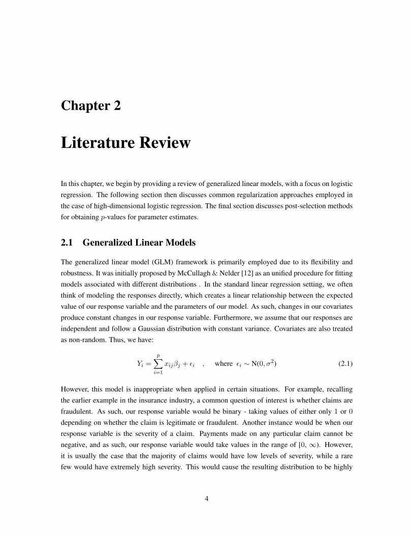
In this chapter, we begin by providing a review of generalized linear models, with a focus on logistic

regression. The following section then discusses common regularization approaches employed in

the case of high-dimensional logistic regression. The final section discusses post-selection methods

for obtaining p-values for parameter estimates.

2.1 Generalized Linear Models

The generalized linear model (GLM) framework is primarily employed due to its flexibility and

robustness. It was initially proposed by McCullagh & Nelder [12] as an unified procedure for fitting

models associated with different distributions . In the standard linear regression setting, we often

think of modeling the responses directly, which creates a linear relationship between the expected

value of our response variable and the parameters of our model. As such, changes in our covariates

produce constant changes in our response variable. Furthermore, we assume that our responses are

independent and follow a Gaussian distribution with constant variance. Covariates are also treated

as non-random. Thus, we have:

Yi =p∑i=1

xijβj + εi , where εi ∼ N(0, σ2) (2.1)

However, this model is inappropriate when applied in certain situations. For example, recalling

the earlier example in the insurance industry, a common question of interest is whether claims are

fraudulent. As such, our response variable would be binary - taking values of either only 1 or 0depending on whether the claim is legitimate or fraudulent. Another instance would be when our

response variable is the severity of a claim. Payments made on any particular claim cannot be

negative, and as such, our response variable would take values in the range of [0, ∞). However,

it is usually the case that the majority of claims would have low levels of severity, while a rare

few would have extremely high severity. This would cause the resulting distribution to be highly

4

skewed. As such, in either of the two cases presented, the assumption that our response variable

follows a Gaussian distribution is out of place.

On the other hand, a generalized linear model can be employed to much success in either of the

aforementioned situations, due to its capability to assume any arbitrary distribution that is part of the

exponential family. Consequently, this displays its flexibility and ease of accommodating situations

that normally require different approaches. Furthermore, as opposed to the linear regression setting

where we model Yi directly as in (2.1), we seek to model E(Yi) in the generalized linear model

context. The ordinary liner model in (2.1) can be described in the following way,

µi = E[Yi] =p∑j=1

xijβj (2.2)

In the generalized linear model setting, we model a function of the mean of our response variable

instead. That is to say, the relationship between a function of µi and the parameters is linear. We

assume:

g(µi) =p∑i=1

xijβj = ηi (2.3)

Here, g is called the link function, and the most common choice for g in the logistic regression

setting is that of the logistic link function (also known as the logit link), which can be expressed as

follows:

g(πi) = log(

πi1− πi

)=

p∑i=1

xijβj (2.4)

Notice that for binary data Yi, we have µi = E(Yi) = P(Yi = 1|xi) = πi, where πi is the probability

of observing a success. The link function also happens to be one of the three components of a

generalized linear model, namely:

(i) The distribution of Yi is in the exponential family - that is, the density of Yi can be written in

the form:

fYi(yi; θi) = exp{a(yi)b(θi) + c(θi) + d(yi)} (2.5)

If b(θi) is the identity function, as we now assume, the model is said to be in canonical form.

(ii) Our covariates and coefficients produce a linear predictor η.

ηi =p∑i=j

xijβj (2.6)

5

(iii) There exists a link funtion g, which we require to be differentiable and monotonic on the

range of µi = E(Yi), such that:

µi = g−1(ηi) (2.7)

Also, notice that µi =∫yif(y; θi)dyi is a function of the parameter θi.

Sometimes, (2.6) is called the random component of a generalized linear model, whereas (2.7)

is called the systematic component. The link function then acts as the bridge that describes the

relationship between the two.

Now, consider the generalized linear model setting where our response variable follows a bino-

mial distribution, and a logit link function is employed. Notice that if we write out the likelihood in

the form shown in (2.5), with b the identity so that (2.5) is in canonical form, we would obtain the

following:

L(θ1, . . . , θn;y) =n∏i=1

exp{a(yi)θi + c(θi) + d(yi)}. (2.8)

However, this likelihood is not expressed in terms of the coefficients β that we wish to estimate.

Retaining the notation that πi = P(Yi = 1|xi) , notice that if we explicitly write out the probability

mass function, we set:

L(θ1, . . . , θn;y) =n∏i=1

πiyi(1− πi)1−yi

=n∏i=1

exp{yilog

(πi

1− πi

)+ log(1− πi)

}.

(2.9)

Thus, we have a(yi) = yi , θi = ηi = log(

πi1−πi

), c(θi) = log(1 − πi) and d(yi) = 0. Sub-

sequently, by making use of the identity provided by our link function in (2.4), we rewrite (2.9)

as:

L(β;y) =n∏i=1

exp{yilog

(πi

1− πi

)+ log(1− πi)

}=

n∏i=1

exp{yiηi + log

( 11 + eηi

)}=

n∏i=1

exp{yi

p∑j=1

xijβj + log( 1

1 + e∑

jxijβj

)}(2.10)

6

which is now in terms of β. Naturally, the log-likelihood follows as:

`(β;y) = logL(β;y) = log

(n∏i=1

exp{yilog

(πi

1− πi

)+ log(1− πi)

})

=n∑i=1

yi

p∑j=1

xijβj +n∑i=1

log( 1

1 + e∑

jxijβj

)

=n∑i=1

yi

p∑j=1

xijβj −n∑i=1

log(

1 + e∑

jxijβj

)

=p∑j=1

Tjβj −n∑i=1

log(

1 + e∑

jxijβj

),

(2.11)

where Tj = ∑ni=1 yixij . Taking derivatives with respect to β of our log-likelihood function, setting

them equal to 0 and solving, then provides us with the desired coefficient estimates. However, in

this case, the maximum likelihood estimate of β does not have a closed form solution, and as such,

numerical methods have to be employed.

For completeness, we note that the first derivative of the log-likelihood function is called the

score function, and its expected value is 0. To show this, we consider the logistic regression setting

as shown above in (2.11). We begin by taking its derivative, which results in the following:

∂

∂βk

[ p∑j=1

Tjβj −n∑i=1

log(

1 + e∑

jxijβj

)]

=n∑i=1

yixik −n∑i=1

xike∑

jxijβj

1 + e∑

jxijβj

=n∑i=1

yixik −n∑i=1

xikπi

=n∑i=1

xik(yi − πi

).

(2.12)

Above, we made use of the fact that πi = eηi1+eηi , where ηi = ∑p

j=1 xijβj . Notice that solving for

the zeros of the resulting score function in (2.12) would provide us with the maximum likelihood

estimate of β. Now, since each individual yi is an independent Bernoulli random variable, we have

E(yi) = πi. As such, taking the expected value of (2.12) provides us with the desired result of:

E[ n∑i=1

xik(yi − πi

)]=

n∑i=1

xik(πi − πi

)= 0 .

(2.13)

7

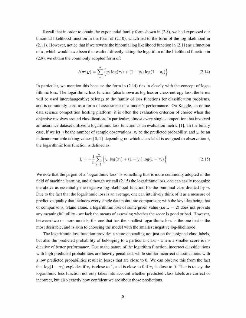
Recall that in order to obtain the exponential family form shown in (2.8), we had expressed our

binomial likelihood function in the form of (2.10), which led to the form of the log likelihood in

(2.11). However, notice that if we rewrite the binomial log likelihood function in (2.11) as a function

of π, which would have been the result of directly taking the logarithm of the likelihood function in

(2.9), we obtain the commonly adopted form of:

`(π;y) =n∑i=1

{yi log(πi) + (1− yi) log(1− πi)

}(2.14)

In particular, we mention this because the form in (2.14) ties in closely with the concept of loga-

rithmic loss. The logarithmic loss function (also known as log loss or cross-entropy loss; the terms

will be used interchangeably) belongs to the family of loss functions for classification problems,

and is commonly used as a form of assessment of a model’s performance. On Kaggle, an online

data science competition hosting platform, it is often the evaluation criterion of choice when the

objective revolves around classification. In particular, almost every single competition that involved

an insurance dataset utilized a logarithmic loss function as an evaluation metric [1]. In the binary

case, if we let n be the number of sample observations, πi be the predicted probability, and yi be an

indicator variable taking values {0, 1} depending on which class label is assigned to observation i,

the logarithmic loss function is defined as:

L = − 1n

n∑i=1

{yi log(πi) + (1− yi) log(1− πi)

}(2.15)

We note that the jargon of a "logarithmic loss" is something that is more commonly adopted in the

field of machine learning, and although we call (2.15) the logarithmic loss, one can easily recognize

the above as essentially the negative log-likelihood function for the binomial case divided by n.

Due to the fact that the logarithmic loss is an average, one can intuitively think of it as a measure of

predictive quality that includes every single data point into comparison; with the key idea being that

of comparisons. Stand alone, a logarithmic loss of some given value (i.e L = 2) does not provide

any meaningful utility - we lack the means of assessing whether the score is good or bad. However,

between two or more models, the one that has the smallest logarithmic loss is the one that is the

most desirable, and is akin to choosing the model with the smallest negative log-likelihood.

The logarithmic loss function provides a score depending not just on the assigned class labels,

but also the predicted probability of belonging to a particular class - where a smaller score is in-

dicative of better performance. Due to the nature of the logarithm function, incorrect classifications

with high predicted probabilities are heavily penalized, while similar incorrect classifications with

a low predicted probabilities result in losses that are close to 0. We can observe this from the fact

that log(1 − πi) explodes if πi is close to 1, and is close to 0 if πi is close to 0. That is to say, the

logarithmic loss function not only takes into account whether predicted class labels are correct or

incorrect, but also exactly how confident we are about those predictions.

8

2.2 Regularization Approaches

Regression methods that involve regularization, also known as penalized regression, are a class of

techniques that place constraints on the size of coefficient estimates through the usage of what is

commonly called a penalty term. Penalized regression is often utilized to address issues of over-

fitting, as well as in situations where we have ill-posed problems - which is exactly the case in

high-dimensions where p > n. Here, we discuss the Lasso, ridge, elastic net and relaxed Lasso

regularization approaches, with more focus being placed on the former two, since the latter half can

be seen as either an extension or generalization of the former.

2.2.1 Lasso

First introduced by Tibshirani in 1996, the Least Absolute Shrinkage and Selection Operator (Lasso)1

is a regression technique that has wide applications across countless different fields. A prominent is-

sue of consideration when dealing with high dimensional data is the process whereby one identifies

the subset of important variables that are ultimately used to fit the model of choice. In this re-

gard, the Lasso performs both regularization through penalizing and shrinking parameter estimates,

and variable selection by being able to shrink parameter estimates to exactly zero. As a result, it

addresses the aforementioned problem.

To begin, we consider the linear regression setting. As before, we let X ∈ Rn×p be our de-

sign matrix, where the ith row of X is xi = (xi1, xi2, . . . xip), and the jth column of X is xj =

(x1j , x2j , . . . xnj)T . We let Y be a vector of n response variables and ε be a vector of indepen-

dently and identically distributed N(0, σ2) variates. This then gives the usual linear model:

Y = Xβ + ε (2.16)

In order to obtain parameter estimates, the Lasso seeks to minimize the residual sum of squares with

the addition of a penalty term:

βL = arg minβ∈Rp

{ 12‖Y −Xβ‖2

2 + λ‖β‖1

}(2.17)

Commonly, we would first center and standardize our covariates - that is to say, we would subtract

the mean of column j from column j for each of the j columns of the design matrix X , and then

scale them to be of unit length. We would then center our response vector Y as well. Doing so

allows us to account for the effect of an intercept term without explicitly defining it in our model;

this is done to avoid penalizing the intercept term. Besides standardizing our design matrix, for the1Henceforth abbreviated as "Lasso", which is the commonly adopted form in recent literature, as opposed to "lasso"

or "LASSO".

9

remainder of this subsection, we also assume that the columns ofX are orthonormal. Here, λ‖β‖1is the penalty term, and λ is known as the tuning parameter; it influences the Lasso solution by

controlling the magnitude of the penalty being imposed on the estimated coefficients. Larger values

of λ drive all coefficients towards zero, and conversely, smaller values of λ allow coefficients to take

values further away from zero.

In order to better illustrate this concept, consider the following. Suppose that we wish to solve

for a closed-form solution of X . The problem at hand that we wish to solve is that of (2.17). Now,

if we expand the terms, we end up with:


{12Y

TY + 12β

Tβ − Y TXβ + λ‖β‖1

}(2.18)

Subsequently, we make use of the least-squares solution provided in (1.4) to rewrite the problem of

interest. Under our previous assumptions, we have:

βls = (XTX)−1XTY = XTY = Y TX (2.19)

By making use of the above identity and discarding the 12Y

TY term since it does not contain β, the

parameter being optimized over, we now frame our problem of interest in the following way:


{12β

Tβ − Y TXβ + λ‖β‖1

}

= arg minβ∈Rp

{ p∑j=1

(12βj

2 − βj βjls + λ|βj |

) }

Now, we are left with an equation that is a function of βj which represents the Lasso solution, and

βjls which represents the least squares solution. Necessarily, in order to minimize this quantity, we

require that the signs of both βj and βj ls be matching - that is to say, if βj ls ≤ 0, βj ≤ 0 has to

follow suit, with the converse being true as well. Otherwise, contrasting signs would cause βjβj ls

to take a negative value, which in turn increases the function that we are trying to minimize.

Finally, if we takes derivatives and solve for βj , while accounting for the fact that the signs of

the least-squares and Lasso solutions have to match, we end up with:

βj = sign(βjls)(|βj

ls| − λ)+, (2.20)

where(|βj

ls| − λ)+

denotes the positive part of(|βj

ls| − λ)

. Looking at (2.20), one can see that

if λ is extremely large, all the Lasso coefficients are likely to be zero. In fact, it is necessarily the

10

case when λ > max|βjls| that all the Lasso coefficients are exactly zero. Conversely, if we have

λ = 0, we recover the least-squares solution.

Now, instead of fixing a lambda and solving the Lasso problem, one can think about how the

Lasso problem hangs together as a whole. Although it might not appear to be apparent, we note that

the solution path of β is a piecewise linear function of λ, with knots λ1 ≥ λ2 ≥ . . . ≥ λr ≥ 0. A

convincing discussion on this is provided by Tibshirani et. al. [18]. Between any 2 consecutive knots

λk and λk+1, there exists an active setA that remains the same for all values of λ between those two

knots; any given knot λk represents the entry or departure of a particular variable from the current

Lasso active set. We define the Lasso active set A as the support set of the Lasso solution β(λ),

denoted as A = supp(β)⊆ {1, . . . , p}, where we have βk = 0 if and only if k /∈ A. Intuitively,

suppose that we now initiate the penalty parameter at λ = ∞, such that all coefficients are exactly

zero. As such, it follows that the solution of β(∞) has no active variables. If we were to then slowly

reduce λ and attempt to move the first β away from zero, either in the positive or negative direction,

there will come a point when a particular value of λ accomplishes this - and this happens precisely

at the knot λ1. The Lasso solution will admit a covariate with a non-zero coefficient which enters

the active set, and subsequently becomes the first variable to enter the active set along the Lasso

solution path. As we progress to each subsequent knot, variables can be either added or deleted

along the way, and this ultimately forms the complete Lasso solution path.

Until now, we have been discussing the properties and applications of the Lasso in the standard

linear model setting. However, it is commonly the case that the Lasso is in fact extended to, and

applied in the generalized linear model setting. Instead of minimizing the residual sum of squares,

we now transition over to minimizing our objective function - which is formed from the negative

log-likelihood function after appending a penalty term. More precisely, we define the new function

as{− `(β;y) + λ‖β‖1

}, and estimate β using:


{− `(β;y) + λ‖β‖1

}(2.21)

where `(β;y) is the log likelihood function and ‖β‖1 = ∑pj=1 |βj | is the `1-norm of β. To consider

the logistic regression setting, we would simply replace `(β;y) with the result obtained in (2.11).

2.2.2 Ridge Regression

Ridge regression was initially introduced as a solution directed at addressing the issue of non-

orthogonal and ill-posed problems [8], which may arise as a result of multi-collinearity - or in our

case, high-dimensionality. Similar to the Lasso, in the ridge regression setting, coefficient estimates

are shrunk towards zero as the penalty parameter λ increases. However, ridge coefficient estimates

never reach exactly zero (unless λ = ∞), and this provides a stark contrast with the Lasso through

the inherent implication that ridge regression is incapable of performing variable selection.

11

Again, we begin by considering the standard linear regression model:

Y = Xβ + ε (2.22)

Now, instead of a `1 penalty in the case with the Lasso, the ridge objective function imposes a

squared penalty. Our ridge regression estimates are defined by:

βridge = arg minβ∈Rp

{‖Y −Xβ‖2

2 + λ‖β‖22

}(2.23)

where ‖β‖2 =√∑p

j=1 β2j is the `2-norm of β. As before, we retain the notion of not penalizing

the intercept term as we had done in Section 2.1.1 for the Lasso. However, unlike the Lasso, ridge

regression does not require the assumption of an orthogonal design matrix X to provide a closed-

form solution. To illustrate this, we solve for the ridge solution, beginning by first expanding the

equation in (2.23). This gives us:

βridge = arg minβ∈Rp

{(Y −Xβ)T (Y −Xβ) + λβTβ

}= arg min

β∈Rp

{Y TY − Y TXβ − βTXTY + βTXTXβ + λβTβ

} (2.24)

Subsequently taking derivatives and solving yields the following normal equation,

XTY =(XTX + λI

)β (2.25)

which leads to the estimate:

βridge =(XTX + λI

)−1XTY (2.26)

By introducing the addition of positive quantities to the diagonal elements ofXTX , the result-

ing new matrix of(XTX + λI

)−1 will always be invertible for some given value of λ, regard-

less of whether XTX is initially invertible. Consider the following simple illustration. For some

given matrix Q, we say that Q is singular if and only if there exists some vector v 6= 0 such that

Qv = 0. Necessarily,Qv = 0 translates to the fact that vTQv = 0 has to be true as well. As such,(XTX +λI

)is singular if and only if vT

(XTX +λI

)v = 0 for some v 6= 0. However, if v 6= 0,

vT(XTX + λI

)v = (Xv)T (Xv) + λvTv > 0 (2.27)

is always true provided that λ > 0, since (Xv)T (Xv) and vTv cannot take negative values. As

such,(XTX + λI

)cannot be singular, and hence is always invertible for all λ > 0. Furthermore,

although we introduce bias into ridge estimators through the addition of positive quantities to the

12

diagonal elements ofXTX , ridge estimators are always capable of achieving a lower mean squared

error when compared to the unbiased least-squares estimator [8].

As before, if we were to transition over to the generalized linear model setting, we would have

an objective function that is composed of the negative log likelihood and a penalty term. Now

however, the ridge imposes a `2 penalty, as opposed to the `1 penalty in the case of the Lasso; our

ridge estimator is:

βridge = arg min{− `(β;y) + λ‖β‖22

}(2.28)

2.2.3 Elastic Net

The elastic net was introduced by Zou and Hastie as a regularization approach that is often capable

of outperforming the Lasso, especially in the case where the number of predictors is significantly

larger than the sample size (i.e. p >> n), while retaining a similar sparsity of representation [12].

The elastic net can be seen as a linear combination of the ridge and Lasso approaches, since it

imposes both an `1 and `2 penalty when optimizing its objective function, as shown below.

β = arg min{− `(β;y) + λ1‖β‖1 + λ2‖β‖2

}(2.29)

This can in fact be seen as a generalization of both the ridge and Lasso, since we would be able

to recover either of the former if either λ1 or λ2 happened to be zero respectively. Although the

introduction of two penalty terms enables better model robustness, we also recognize it as one of

the more apparent drawbacks of the elastic net, since it requires tuning of an additional parameter

as compared to other methods.

2.2.4 Relaxed Lasso

The relaxed Lasso was introduced by Meinshausen [13] as a solution that extended, and addressed

shortcomings of, the Lasso. It was primarily targeted at improving the bias of Lasso coefficients, as

well as the Lasso’s tendency to select noise variables if the penalty parameter was selected through

cross-validation. To implement the relaxed Lasso, a 2-step procedure is followed.

(1) Fit the model with the Lasso penalty, and identify the non-zero coefficients.

(2) Refit the same model without the Lasso penalty, while using only the covariates that corre-

spond to the non-zero coefficients identified in (1).

Due to the fact that Lasso estimates are shrunk, they often happen to be biased towards zero. By

choosing to refit the same model with the covariates selected from the Lasso model, but without

penalizing the coefficients, we are in a sense "relaxing"’ the results we would obtain if we had

simply just the Lasso model on its own.

13

2.3 Post Selection Inference

In the context of post selection inference using penalized regression, traditional methods are inca-

pable of providing valid confidence intervals or p-values for coefficient estimates. In this section, we

discuss two different approaches for obtaining p-values for coefficient estimates for the penalized

regression approaches presented in Section 2.2.

2.3.1 Covariance Test

Specifically in the case of the linear regression model with Lasso regularization, Lockhart et. al.

[10] propose a covariance test statistic that can be used for assessing the significance of the covariate

that enters the present Lasso model at a given stage along the Lasso solution path. Given moderate

assumptions on the predictor matrix X , it is shown that the covariance test statistic, denoted as Tk,

asymptotically follows an exponential distribution under the null hypothesis that the current Lasso

fit contains all truly active variables. Let k be the current step of the Lasso solution path, A be the

current active set of covariates (as defined in Section 2.2.1) and XA be the columns of X that are in

A. Then, the proposed covariance test statistic is:

Tk = (⟨y,Xβ(λk+1)

⟩−⟨y,XAβA(λk+1)

⟩)/σ2 (2.30)

Here, β(λk+1) is the solution of the Lasso problem at λ = λk+1 while using covariates A ∪ {j},with A being the current active set and covariate j entering at step k (i.e. at λ =λk). On the other

hand, β(λk+1) is the Lasso solution while only using the current active covariates, at λ = λk+1.

The test statistic is then obtained from the inner product of [Xβ(λk+1)−XAβA(λk+1)] with y, and

intuitively represents an uncentered covariance calculation, which provided the motivation for its

name.

Notice that the manner in which we have written (2.30) requires the assumption that σ2 is

known. However, in practice, σ2 is in fact often unknown and will have to be estimated by some

value of σ2 − and the procedure for doing so differs depending on the given sample size n and

number of predictors p. A common choice when n > p is to estimate σ2 by the mean squared error,

and in this case, the covariance test statistic in (2.30) has an asymptotic F-distribution under the null

hypothesis [10]. In the case of p ≥ n, Lockhart et. al suggest estimating σ2 from the least squares

fit on the support of the model selected by cross-validation, but also comment that this approach is

not supported by rigorous theory and will be addressed in future work.

14

2.3.2 p-value Estimation from multi-sample splitting

An alternate approach based on sample splitting is proposed by Wasserman and Roeder [21] for

high-dimensional linear models, with related work subsequently done by Buhlmann and Mandozzi

[3]. In particular, Buhlmann et. al. [2] provide a multi sample-splitting approach that is generalized

from the work done by Wasserman and Roeder. The proposed multi sample-splitting method is

capable of constructing estimated p-values for both the hypothesis testing of individual covariates,

H0,j : βj = 0 vs. HA,j : βj 6= 0 ,

as well as tests involving groups of covariates together.

H0,G : βj = 0 , ∀j ∈ G vs. HA,G : βj 6= 0 for at least some j ∈ G

In the context of multiple testing of H0,j : βj = 0, the algorithm seeks to control the family-wise

error rate P(V > 0), where V represents the number of false positives; a false positive being an

incorrect rejection of the null hypothesis. That is to say, V is the number of βj , where j ∈ {1 . . . p},that are mistakenly determined to be significantly different from zero. The specific steps of the multi

sample-splitting approach are as follows:

Algorithm 1: Multi-sample splitting method for obtaining p-values

Steps:

1. Given a sample of size n, randomly split the sample into two sets I1 and I2, where |I1| =bn/2c and |I2| = n− bn/2c.

2. Select covariates S ∈ {1, . . . , p} based on our modeling approach using I1.

3. Consider the reduced set of covariates in I2 by only retaining those selected in S. Compute

p-values pj for H0,j , j ∈ S, using standard least squares estimation.

4. Correct the p-values for multiple testing with pj,corr = min (|S| · pj , 1).

5. Repeat the steps 1-4 for B = 100 times and aggregate the results.

We do not present the exact aggregation method mentioned in step 5 here, due to the fact that it is

lengthy in nature and requires substantial discussion that does not align with the focus of this paper.

Details of the aggregation method may be found in Buhlmann et. al’s paper [2] .

15

Chapter 3

Applied analysis of regularizationapproaches under varying n, p

conditions.

In this section, we aim to provide applied analysis examples utilizing the different regularization

approaches discussed in Section 2.2 with real-world datasets. In particular, we will be considering

the different cases of:

1. n > p ;

2. n < p ; and

3. n = p .

We begin by providing a description of the datasets used, followed by a brief discussion on sample

splitting between test and training sets, and approaches to choosing appropriate values for tuning

parameters. We then fit logistic regression models to our datasets with the four different regular-

ization methods discussed in Section 2.2, under the three varying n, p conditions shown above, and

present results with accompanying discussion.

16

3.1 Datasets

For the purposes of this illustration, we utilize 2 different datasets in order to accommodate the

varying conditions we wish to investigate. A birth weight dataset will be used in the case where

n > p, while a riboflavin dataset will be used in the cases where n = p and p > n.

3.1.1 Birth Weight

The first dataset in consideration is the Baystate Medical Center birth weight dataset, which contains

n = 189 samples and p = 8 predictors that are believed to be risk factors associated with low birth

weight. The response variable is dichotomous, and acts as an indicator of the presence or absence

of low birth weight. The dataset is obtained from the MASS R package [19].

3.1.2 Riboflavin

The second dataset used in this example is the riboflavin dataset, which contains measures of gene

expression on n = 71 sample observations of p = 4088 predictor genes. The response variable in

this case is continuous, and represents the log-transformed riboflavin production rate. This dataset

is contained in the hdi R package [4].

3.1.3 Test and Training Splits

Before we evaluate any given approach, we first partition the sample observations of our dataset into

test and training sets. The training set is defined as the subset of our original sample observations

that is utilized in building a relationship between our predictors and response variable through our

desired modeling approach. Conversely, the test set is utilized as a means of validation and assess-

ment of the performance of the model built from our training set. As such, one would commonly

train a model on the training set, and subsequently evaluate the model’s performance on the test set

to assess the suitability of the employed approach.

However, an important question of consideration is how exactly one would split the original

dataset, and particularly so in cases where the sample size is not very large. There exists a trade-

off between retaining more information during the process of building the model, and leaving out

information to be used during the performance validation of the built model. Dobbin et. al. [5]

state that for sample sizes n close to or greater than 100, a 1/3rd to 2/3rd split between the test

and training sets often happens to be close to optimal in terms of prediction accuracy, with smaller

sample sizes requiring larger proportions assigned to the training set. As such, given that we have

n = 189 in the case of the birth weight dataset, we choose to employ the proposed 1/3rd (n1 = 63)

to 2/3rd (n2 = 126) split. Conversely, due to the fact that the size of the riboflavin dataset is smaller

than the recommended level, we choose to allocate a higher proportion to the training set - settling

on a 70-30% split between the training (n1 = 50) and test set (n1 = 21) respectively.

17

3.2 Setup

Below, we describe the setup for the varying n, p conditions that we investigate. For each of the

cases, we fit the following models and assess their performance.

(a) Logistic regression model with Lasso penalty;

(b) Logistic regression model with ridge penalty;

(c) Logistic regression model with elastic net penalty; and

(d) Relaxed Lasso.

All aforementioned models were built with the statistical software R [16] using the glmnet package

[9]. However, in the case of the elastic net, due to the fact that it requires tuning of more than a

single parameter, additional functionality provided by the caret package [7] was utilized as well.

3.2.1 Choosing the Tuning Parameter

An important consideration when fitting penalized regression models is choosing a value for the

tuning parameter(s). For the applied example in this section and for the remainder of this paper, we

will be making use of 10-fold cross validation as the approach of choice for selecting a value for

our tuning parameter. The procedure in question consists of splitting the dataset into 10 equal-sized

subsamples, before collectively fitting the desired model on 9 subsamples (i.e. 90% of the data is

used as the training set) and evaluating the model’s performance on the remaining single subsample

(i.e. 10% of the data is used as the validation set). This is then repeated for all 10 possible cases,

where each of the 10 subsamples would be used once as the validation set. The value of λ that

results in the lowest mean square error rate is then chosen.

3.2.2 Case where n > p

Here, we make use of the Baystate Medical Center birth weight dataset, where we have n = 189sample observations and p = 8 predictors. The response variable is binary. As mentioned in Section

3.1.3, we begin by splitting our sample observations into separate test and training sets according to

the proposed optimal split by Dobbin et. al. [5]. We then proceed to fit each of the aforementioned

models, while retaining the same training and test sets.

18

3.2.3 Case where n < p

In this case, we make use of the riboflavin dataset, which has n = 71 sample observations and

p = 4088 predictors. Once again, we split the sample observations into test and training sets

before applying the desired fitting approaches. However, due to the fact that the response variable

in consideration is in fact continuous, for the purpose of illustrating the workings of the proposed

fitting approaches in a logistic regression setting, we choose to dichotomize it into binary responses

using the mean production rate of the response as the point of division. As a result, of the original

71 sample observations, 40 observations which were greater than the mean were assigned to one

class, while the remaining 31 were assigned to another.

3.2.4 Case where n = p

In this final scenario, due to the difficulty of finding real-world datasets that have exactly the same

number of sample observations and predictors, we seek to artificially create such a result by making

use of the riboflavin dataset. We select the 50 covariates that have the highest correlation with the

response variable, and retain only the columns of our design matrix X that correspond to those

covariates. Recall that back in Section 3.1.3, a split of n1 = 50 and n2 = 21 was decided on

between the training and test sets. Now, since we are building our models using only the training

set, we in fact have the desired scenario of n = p = 50. Subsequently, we dichotomize the response

variable as we had done for the case where p > n.

3.3 Variable Selection

In this section, we focus on examining the variables selected by the penalized regression methods

employed in the two cases where p ≥ n (i.e. when we are in a high-dimensional setting). In both

cases, we dichotomized the continuous response vector of the riboflavin dataset based on its own

mean, before partitioning the riboflavin dataset into test and training sets based on a single random

split. All models were then fit on only the training set, and subsequently evaluated on the test set.

Values of penalty parameters were chosen via 10-fold cross validation. Due to the fact that the ridge

model does not perform variable selection, and the relaxed Lasso selects the same variables as the

Lasso, we only look at the results obtained from the Lasso and elastic net. In total, the Lasso selects

21 non-zero coefficients in the case where p > n and 11 when p = n. On the other hand, the elastic

net selected 77 non-zero coefficients in the case where p > n and 27 when p = n. Table 3.1 shows

the first 5 covariates to enter the Lasso and elastic net models, as well as their estimated coefficients.

19

Table 3.1: The estimated coefficients of the first 5 covariates to enter the Lasso and elastic net fitsare shown. The covariate# represents the column position of the covariate in the design matrixX

p = n p > n

Covariate # Estimate Covariate # Estimate

Lasso1285 1.468 1285 0.1221123 0.999 1123 0.1094003 -0.590 4003 -0.0782384 -0.353 4006 0.0231516 0.314 2384 -0.023

Elastic Net1123 0.792 150 -0.0881516 0.366 1123 0.0791284 0.358 1861 0.0784003 -0.231 4003 -0.0754004 -0.199 4004 -0.075

We observe that coefficient estimates were much smaller across the board in the case where p > n

when compared to p = n, and elastic net coefficient estimates were always smaller than those

obtained from the Lasso. Furthermore, the first 5 covariates selected by the Lasso and elastic net

differ quite significantly as well.


Here, we apply the covariance test to determine the significance of the variables that enter the Lasso

model. Table 3.2 shows the drop in covariance induced by each of the first 5 covariates as they

enter our model with the Lasso penalty built on only the training set, as well as their corresponding

p-values, in the case where p > n. Table 3.3 shows the drop in covariance and p-values associated

with the first 5 covariates to enter our model with the Lasso penalty, but instead fitted on the full

riboflavin dataset (without partitioning into training/test sets).

Table 3.2: The p-value and drop in covariance are shown for the first 5 covariates selected using theLasso in the case where p > n.

Predictor # Drop in Covariance p-value

1285 0.691 0.5011123 0.364 0.6954003 0.521 0.5942384 0.160 0.9671516 0.469 0.626

20

Table 3.3: The p-value and drop in covariance are shown for the first 5 covariates selected using theLasso in the case where p > n.

Predictor # Drop in Covariance p-value

1285 0.691 0.5011123 0.364 0.6954003 0.521 0.5942384 0.160 0.9671516 0.469 0.626

Here, we observe that none of the first 5 covariates to enter the Lasso model were determined to

be significant. We also notice that the results we obtained for the Lasso when using the full riboflavin

dataset differs from those obtained by Buhlmann et. al. [2], where they had covariates 1278, 4003,

1516, 2564, 1588 entering the model in that particular order. Necessarily, this is attributed to the

fact that we had dichotomized the response variable and fitted a logistic regression model for the

case in Table 3.2, as opposed to the standard linear approach that was employed by Buhlmann et.

al. Furthermore, we partitioned our data into test and training sets, and only fitted our model on the

training set.

3.4 Model Evaluation

In this section, we will be examining some of the commonly used metrics for model evaluation that

are applicable to binary classification - namely, prediction accuracy, log loss, and area under the

curve. We apply these evaluation metrics under the setups with varying n, p conditions described in

Section 3.2. Recall that for each of the 3 different n, p conditions, a different dataset was used to

train the model. For n > p, we used the birth weight dataset as described in Section 3.2.2, whereas

for p > n, we used the riboflavin dataset with all p = 4088 predictors as described in Section 3.2.3.

Finally, for the case where n = p, we used a subset of the riboflavin data by choosing the 50 most

highly correlated variables with the response as described in Section 3.2.4.

3.4.1 Prediction Accuracy

We evaluate the prediction accuracy of any given method as the proportion of predictions that match

the actual response values in the test set, while using the model built from the training set. Due to

the fact that the response variable is binary, we made assignments during the prediction process

depending on whether the probability of a sample observation belonging to a certain class exceeded

0.5 - that is to say, observations were assigned to whichever class label had a higher fitted probability.

Table 3.4 shows the prediction accuracies of our classifiers which were built on the training set, when

evaluated on the test set, based on a single random split between training and test sets.

21

Table 3.4: Prediction accuracies for each of the four different regularization approaches under thethree varying n, p conditions. The birth weight dataset was used in the case of n > p, while theriboflavin dataset was used for the case where p > n. The final case of n = p made use of a subsetof the riboflavin dataset.

Lasso Ridge Elastic Net Relaxed Lasso

n > p 0.97 0.86 0.90 0.94p > n 0.90 0.86 0.86 0.86n = p 0.86 0.90 0.90 0.86

We observe that the Lasso outperformed the other methods in the cases where n > p and p > n, and

that the Lasso always performed at least as well as the relaxed Lasso. However, all of the methods

perform decently well, and we are unable to say if any is significantly different from another.

3.4.2 Logarithmic Loss

Here, we evaluate the logarithmic loss (hence abbreviated as log loss), as described in Section 2.1,

of the classifications obtained from our models when applied on the test set. Table 3.5 shows the

resulting log loss scored derived from the penalized regression models fitted, under the varying n, p

conditions.

Table 3.5: Logarithmic loss scores are shown for each of the four different fitting approaches underthe three different n, p conditions.


n > p 0.067 0.303 0.167 1.326p > n 0.454 0.373 0.368 0.573n = p 0.134 0.692 0.257 0.545

We observe that the relaxed Lasso consistently had the largest log loss score among the various

approaches investigated, and since it is desirable to minimize this quantity, the relaxed Lasso is the

worst performing method in this regard. On the other hand, besides the case where p > n, the Lasso

regularization always resulted in the smallest log loss score among the four.

22

3.4.3 Receiver Operating Characteristic Curves

The receiver operating characteristic (ROC) curve shows the trade-off between the true positive rate

and the false positive rate of a binary classifier. The true positive rate, also known as sensitivity,

measures the proportion of positives that are correctly classified as positives. Conversely, the false

positive rate measures the proportion of positives that are incorrectly classified as so (which are

in fact negatives). An ROC curve is then obtained by plotting the true positive rate on the y-axis,

against the false positive rate on the x-axis.

A perfect classifier would have an ROC curve that extends vertically from 0 to 1, yielding a

point at (0, 1), and then horizontally across - hence encompassing the entirety of the area in the

unit square. Thus, the area under the curve (AUC) acts as a measure of the performance of a given

model, with values closer to 1 being more ideal. An AUC of 0.5, which is depicted by a 45 degree

line from the origin, represents what one would achieve purely by randomly guessing the outcomes.

As such, classifiers that produce an AUC ≤ 0.5 essentially provide no meaningful utility, since one

could easily achieve similar performance by pure guessing. Also, notice that the point of (0, 1)represents a perfect classification, due to the fact that the true positive rate is 100%, and the false

positive rate is in fact 0% at that specific location.

Figure 3.1 shows the ROC curves for each of the four different fitting approaches of interest in

the case where n > p, while utilizing the birth weight dataset. Subsequently, Figures 3.2 and 3.3

show the ROC curves for each of the different fitting approaches in the cases where we have p > n

and n = p respectively, for the riboflavin dataset. All of these figures are based on the classifications

of the test set using the classifiers built and fitted on the training data.

23

(a) Lasso (b) Ridge

(c) Elastic Net (d) Relaxed Lasso

Figure 3.1: Receiver operating characteristic (ROC) curves are shown for each of the following:(a) logistic regression with Lasso penalty, (b) logistic regression with ridge penalty, (c) logisticregression with elastic net penalty, and (d) the relaxed Lasso, in the case where n > p using thebirth weight dataset. The ROC curve shows the tradeoff between the true positive rate and falsepositive rate for a binary classifier, and in particular, the perfect classifier would have a ROC curvethat extends vertically from 0 to 1 and horizontally across from 0 to 1 as well, hence maximizingthe area under the curve.

24

(a) Lasso (b) Ridge


Figure 3.2: Receiver operating characteristic (ROC) curves are shown for each of the following:(a) logistic regression with Lasso penalty, (b) logistic regression with ridge penalty, (c) logisticregression with elastic net penalty, and (d) the relaxed Lasso, in the case where p > n using theriboflavin dataset.

25

(a) Lasso (b) Ridge


Figure 3.3: Receiver operating characteristic (ROC) curves are shown for each of the following:(a) logistic regression with Lasso penalty, (b) logistic regression with ridge penalty, (c) logisticregression with elastic net penalty, and (d) the relaxed Lasso, in the case where p = n using a subsetof the riboflavin dataset.

26

Chapter 4

Simulation Study

Through employing a simulation study, we seek to gauge and compare the performance of the

various penalized regression methods, as well as to quantify uncertainty regarding the coefficient

estimates obtained from them. The general idea behind running such simulations revolves around

first randomly generating pseudo data by sampling from some specified probability distribution.

One would then compute the statistics of interest using the generated data, and finally aggregate

the results in some manner after repeating the process for some large number of iterations. The

purpose of our simulation study is directed towards investigating the workings of regularized logistic

regression in high dimensions, and we will be considering three different setups that make use of

the riboflavin dataset.

In this chapter, we begin by describing the general design and setup of our simulation study. We

then report and discuss the results of variable selection and model performance that were obtained

from running the simulation study under the three varying n, p conditions investigated. We end by

tying up loose ends - where we address some of the choices and assumptions made during the study,

provide interpretation of interesting results observed, and highlight the weaknesses discovered in

some methods.

4.1 Simulation Design

Of the three setups in consideration, the first is the case where the number of predictors outnumbers

the number of sample observations, p > n. In this event, we retain the sample size of n = 71 and

number of predictors p = 4088 as they are in the original dataset when generating new data during

the simulation. In the second setup, we investigate the case where the number of predictors equals

the number of sample observations p = n. We will still be making use of the riboflavin dataset,

but only retain the 50 covariates that have the highest correlation with response variable of interest.

In the third and final case, we again take the number of predictors equal to the number of sample

observations p = n, but instead choose our 50 covariates randomly. Now, having described the

various designs, the procedure we undertake is as follows.

27

Algorithm 2: Simulation study with the riboflavin dataset

Steps:

1. Center the response vector Y and the columns of the design matrix X , and scale the

columns ofX by dividing by their standard deviations.

2. Fit the desired penalized regression approach to the original dataset. Identify and select the

first 2 coefficients to enter the model.

3. Using only the columns of the design matrix X that correspond to the earlier 2 coefficients

selected, fit the standard linear model. Denote the coefficient estimates obtained by βs.

4. Generate new Y values based on the standard linear relationship between the covariates and

the response.

Y = Xβ + ε , where ε ∼ N(0, σ2) (4.1)

However, in this case, we use βs in place of β. We retain the design matrixX as it is in the

original riboflavin dataset, but standardized as above. Values of ε are generated by sampling

from a Gaussian distribution with mean 0 and estimated variance σ2, where σ2 = RSSn . We

define the residual sum of squares as RSS = ‖Y −Xβs‖22 . As such, the relationship we

have can in fact be written as:

Y pseudo = Xβs + ε , where ε ∼ N(0, σ2) (4.2)

5. Dichotomize our new response vector Y pseudo based on the mean of our centered response

vector Y . This break point naturally occurs at 0, since Y is centered and has a mean of 0.

6. Apply the desired fitting approaches (which in this case are our penalized logistic regres-

sion models introduced in Chapter 2) to the generated dataset consisting of response vector

Y pseudo and design matrixX , and perform computations of interest. In particular, we look

at:

• Variable selection.

• Model evaluation.

• Hypothesis testing and p-values.

7. Repeat steps 4− 6 for B = 100 times and aggregate results.

28

4.2 Case where p > n

We begin by fitting the a linear model with Lasso regularization to the centered and standardizedX ,

and centered Y of the riboflavin dataset. We then identify the value of λ at the knot where exactly

two non-zero coefficients are admitted into the model - we find that this happens at λ = 0.587, and

the two coefficients of interest correspond to covariates 1278 and 4003. Subsequently, we proceed

to fit the standard linear model with a design matrixXs that only contains those two covariates, and

denote the resulting estimated coefficient vector by βs. Table 4.1 shows the estimated values for

this coefficient vector. Naturally, we observe that the estimate for the intercept term β0 is in fact 0,

since we had priorly centered our design matrix. We then compute the residual sum of squares of

our linear fit divided by n in order to estimate σ2. In this case, we find σ2 = 0.361.

Table 4.1: Coefficient estimates from fitting the standard linear model using only the first 2 covari-ates selected by the Lasso. The response vector Y was centered, while the design matrix X wascentered and standardized.

Coefficient Estimate

β0 0β1278 0.528β4003 -0.472

The fact that 1278 and 4003 were selected is not very surprising if we were to take a look at the

correlation structure of the dataset, which can be observed from the correlation plot shown in Figure

4.1, since the two covariates happen to be highly correlated with the response. We also note that the

first non-zero coefficient to enter the active set of the Lasso always corresponds to the covariate that

has the highest correlation with the response. In fact, we can observe that in this case, covariate 1278happens to be the first to enter the Lasso model and also has the highest correlation (ρ = 0.649)

with the response among all p = 4088 covariates.

Table 4.2: Value of λ used to fit the preliminary Lasso to get coefficient estimates for the simulation,and value of σ used for simulating our response vector.

Parameter Value

λ 0.587σ 0.601

29

Based on βs, we generate values for our response vector Y pseudo, as described in Algorithm-2,

for each iteration of our simulation study. Afterwards, we dichotomize our pseudo response vector

based on the mean of the original response vector Y . Our data is then split into training and test sets;

we fit our models on the training set and evaluate them on the test set. We fit four different logistic

regression models in total, each with one of the regularization approaches discussed in Section 2.2,

and assess their performance in terms of variable selection and model evaluation criteria. Values of

tuning parameters are chosen through 10-fold cross validation.

Figure 4.1: A correlation plot is shown for the five covariates that have the highest correlation withthe response variable, in descending order. Among the five, covariates 1278 and 4003 are the firsttwo to be selected by the Lasso.

30

4.2.1 Variable Selection

Across the B = 100 Monte Carlo samples, we kept track of the number of instances a particular

non-zero coefficient was admitted into the model, as well as its estimate. This was done for the Lasso

and elastic net models, since ridge regression is incapable of performing variable selection and the

relaxed Lasso uses the same selected variables as the Lasso. However, due to the large number

of coefficients in consideration, we chose to review only the five most frequently observed ones in

greater detail. Table 4.3 shows the number of times the five most frequently selected coefficients

were present in the fitted models, as well as their averages and standard deviations. We note that

the averages and standard deviations presented are obtained from only the non-zero values of a

particular coefficient. That is to say, the average and standard deviation given for covariate 1278

in Table 4.3 under the context of the Lasso, are calculated from only the 47 non-zero coefficient

estimates (i.e. the other 53 are exactly 0) among the 100 Monte Carlo samples of the simulation

study.

Table 4.3: The 5 covariates selected most frequently by the Lasso and elastic net with 10-fold crossvalidation across B = 100 samples. For each coefficient, the number of times that variable wasselected is given along with the mean and average of the (non-zero) values. The covariate numberrepresents the column position of the covariate in the design matrix.

Lasso

Covariate # Count Average Standard deviation

1278 47 0.466 0.2854003 40 -0.328 0.2851279 15 0.330 0.284244 14 0.186 0.1971290 14 0.308 0.234

Elastic Net


4003 93 -0.078 0.0411278 92 -0.083 0.0474006 86 -0.061 0.0401279 85 0.065 0.0434004 84 -0.061 0.038

Intuitively, one might already expect covariates 1278 and 4003 to be among the ones that most fre-

quently appear, due to the fact that they were used simulate values for the response vector Y pseudo.

In fact, they can be thought of as the true "correct" variables that we would expect a good perform-

31

ing model to pick out among the many noise variables. We observe that this happens to be true

for both the case of the Lasso and elastic net. Although the elastic net tends to select covariates

1278 and 4003 much more frequently than the Lasso, this does not necessarily imply that the elastic

net is better at identifying the correct variables, since it in fact admits a larger number of non-zero

coefficients across the board. From the B = 100 Monte Carlo samples run, the Lasso selected

7 covariates on average per run, while the elastic net selected 27. Furthermore, we note that the

estimates produced by the elastic net model on average( ¯β4003 = -0.078

)were much smaller than

the true values used to generate the datasets during the simulation(β4003 = -0.472

).

For each sample, we also assessed the statistical significance of any covariate that entered the

Lasso model by making use of the covariance test proposed by Lockhart et. al. At the same time,

we assessed the statistical significance of any covariate that enters the elastic net model by making

use of the sample splitting method proposed by Buhlmann et. al. In doing so, we wish to investigate

whether the models are in fact capable of identifying the correct covariates (i.e. covariates 1278 and

4003 that were used for data simulation), and whether they were determined to be significant. As

such, we examine the following.

(1) How many times were covariates 1278 and 4003 selected by the Lasso model? Of the to-

tal number of times they were selected, how many times did they happen to be statistically

significant?

(2) How many times were covariates 1278 and 4003 the first to enter the Lasso regularized

model? Of the total number of instances, how many times were they statistically significant?

(3) How many times were covariates 1278 and 4003 the second to enter the Lasso regularized

model? Of the total number of instances, how many times were they statistically significant?

(4) How many times were covariates 1278 and 4003 the third or later to enter the Lasso reg-

ularized model? Of the total number of instances, how many times were they statistically

significant?

Table 4.4 shows the number of times where covariates 1278 and 4003 were determined to be statis-

tically significant by the covariance test, out of the total number of times they were selected by the

Lasso model. Subsequently, Table 4.5 shows the number of times where covariates 1278 and 4003

were determined to be significant broken down by the knots at which they enter the Lasso model.

Table 4.6 then shows the number of times that a particular covariate was selected by the Lasso when

covariate 1278 was the first to be admitted into the Lasso solution path, while Table 4.7 shows the

same result for covariate 4003. The correlation structure in the original full riboflavin dataset of

covariates 1278 and 4003, along with the covariates identified in Table 4.6 and Table 4.7, are then

shown in Figure 4.2.

32

Table 4.4: The number of times in 100 Monte Carlo samples that covariates 1278 and 4003 wereselected by the Lasso, as well as the number of instances where they are determined to be statisticallysignificant. Proportions with respect to the total are provided in parentheses.

Lasso

Covariate # Significant Not Significant Total

1278 26 (0.55) 21 (0.45) 474003 16 (0.40) 24 (0.60) 40

Table 4.5: The number of times in 100 Monte Carlo samples that covariates 1278 and 4003 weredetermined to be significant, as well as the total number of instances where they were the first,second, or third or later variable to be selected by the Lasso, respectively. Proportions with respectto the total are shown in parentheses.

First


1278 15 (0.68) 7 (0.32) 224003 6 (0.60) 4 (0.40) 10

Second


1278 0 (0.00) 13 (1.00) 134003 1 (0.11) 8 (0.89) 9

Third


1278 11 (0.92) 1 (0.08) 124003 11 (0.53) 10 (0.47) 21

Interestingly, we observe that both covariates 1278 and 4003 were determined to be not significant

on most instances when they were admitted into the Lasso model second. On the other hand, they

were more likely to be significant when they either entered the model first, third or later onwards.

We direct readers to see Section 4.5.4 for a discussion, where we pursue further investigation into

this matter.

33

Table 4.6: The number of times in 100 Monte Carlo samples that a particular coefficient was ob-served to enter the Lasso regularized model as the second and third non-zero coefficient, whencovariate 1278 enters the model first, ordered by decreasing frequency.

Covariates entering the model 2nd.

4004 1285 1290 Others Total

Counts 9 3 3 7 22

Covariates entering the model 3rd.


Counts 8 3 3 8 22

Table 4.7: The number of times in 100 Monte Carlo samples that a particular coefficient was ob-served to enter the Lasso regularized model as the second and third non-zero coefficient, whencovariate 4003 enters the model first, ordered by decreasing frequency.

Covariates entering the model 2nd.


Counts 3 3 2 2 10

Covariates entering the model 3rd.


Counts 3 3 2 2 10

34

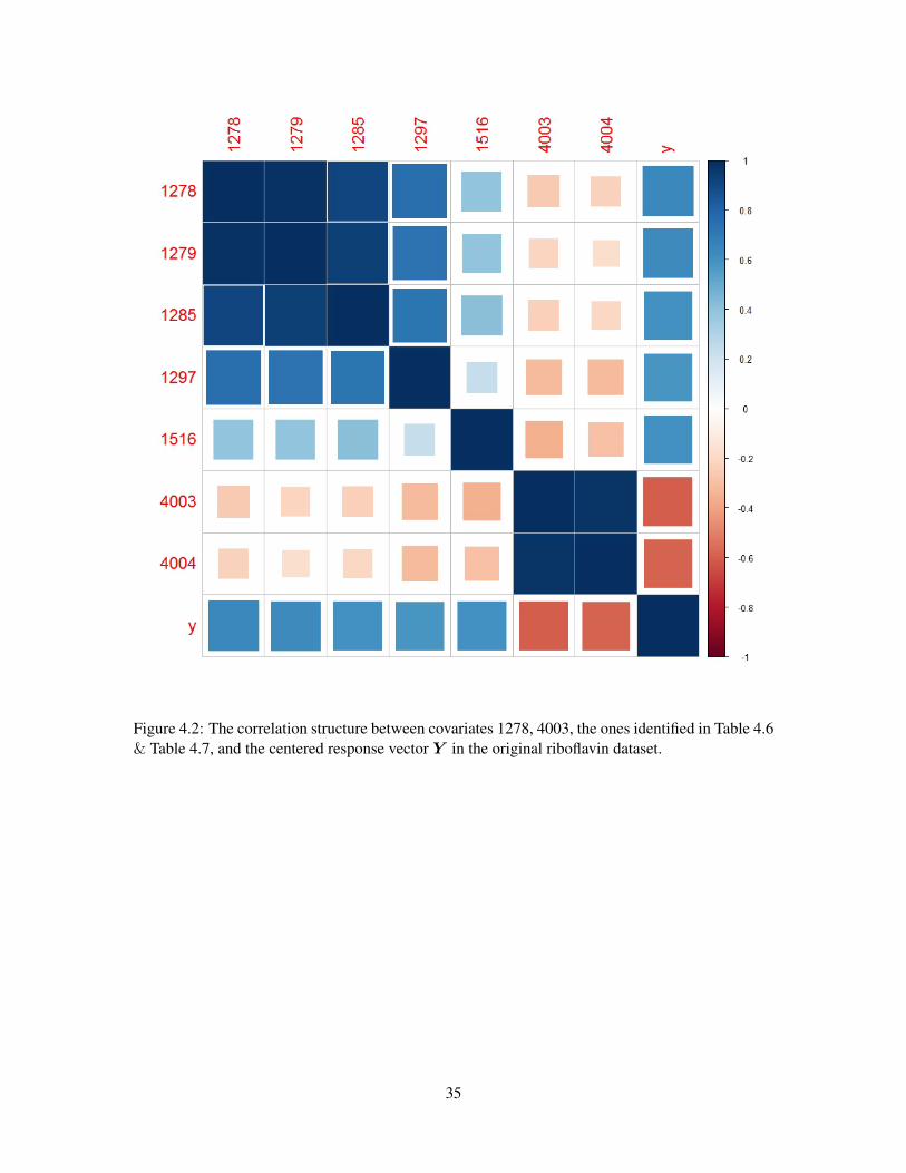
Figure 4.2: The correlation structure between covariates 1278, 4003, the ones identified in Table 4.6& Table 4.7, and the centered response vector Y in the original riboflavin dataset.

35

Similarly, Table 4.8 shows the number of instances where covariates 1278 and 4003 were de-

termined to statistically significant by the sample-splitting method, out of the total number of times

they were selected by the elastic net. However, out of the large number of variables selected by the

elastic net, most were determined to be not significant when the sample-splitting method was ap-

plied to obtain p-values. Across the B = 100 Monte Carlo samples, only 19 unique covariates were

found to be significant. Of these, variable 4003 was declared significant twice and variable 1278

never. In fact, covariate 4003 was the only variable observed to be significant on more than one

occasion. As a result, further partitioning into subsets where either covariate 1278 or 4003 happen

to enter the model first, second, etc. will be skipped due to the small number of significant variables

observed in total.

Table 4.8: The total number of times where covariates 1278 and 4003 were selected by the elasticnet, as well as the number of instances where they were determined to be statistically significant.Proportions with respect to the total are provided in parentheses.

Elastic Net


1278 0 (0.00) 92 (1.00) 924003 2 (0.02) 91 (0.98) 93

36

4.2.2 Model Evaluation

Prediction Accuracy

We assess the prediction accuracy of a given approach by fitting the model on a training set, before

validating it on the test set. Sample splitting between the training and test set will be maintained as

in Section 3.1.3 for the rest of this paper, with n1 = 50 assigned to the training set and n2 = 21assigned to the test set respectively. Model evaluations are all done on the test set. Table 4.9 shows

the average prediction accuracies and standard deviations observed for each of the different models

that were fitted across the B = 100 Monte Carlo samples.

Table 4.9: Average prediction accuracies and standard deviations for each of the four penalizedregression methods investigated during the simulation. Evaluation is done on the test set, using themodel obtained from the training set. A total of B = 100 iterations are run.

Model Average Standard deviation

Lasso 0.710 0.115Ridge 0.682 0.119Elastic Net 0.714 0.105Relaxed Lasso 0.705 0.101

In order to determine if any method yielded a prediction accuracy that was significantly different

from another, we performed paired comparison t-tests with Bonferroni correction; where we are

testing the null hypothesis that the average difference between any two given approach is in fact zero,

against its two-sided alternative. Table 4.10 provides the multiple comparison corrected p-values

obtained. We observe that at the α = 0.05 significance level, none of the prediction accuracies were

determined to be significantly different from each other.

Table 4.10: p-values with Bonferroni correction from paired comparison t-tests between predictionaccuracies obtained from the different penalized regression methods. None are determined to besignificantly different from each other at the α = 0.05 significance level.

Lasso Ridge Elastic Net

Ridge 0.23 - -Elastic Net 1.00 0.11 -Relaxed Lasso 0.36 0.06 1.00

37

Logarithmic Loss

We also evaluate models based on the logarithmic loss of their predictions. Evaluations are done on

the n2 = 21 sample observations of the test set. Recall from (3.2) that the logarithmic loss score

not only depends on the predicted class assignment, but also on the predicted probability of being

in that particular class. Hence, it acts as both a measure on the prediction accuracy of our regression

model and on the confidence of those predictions. Table 4.11 shows the average log loss scores

observed across the B = 100 Monte Carlo samples of our simulation.

Table 4.11: The average and standard deviation of the logarithmic loss scores, across B = 100Monte Carlo samples, for each of the different fitting approaches.



In order to determine if any method yielded a logarithmic loss that was significantly different from

another, we performed paired comparison t-tests with Bonferroni correction. Table 4.12 provides

the multiple comparison corrected p-values obtained.

Table 4.12: p-values with Bonferroni correction from paired comparison t-tests between log lossscores obtain from the different penalized regression methods.


Ridge 1.00 - -Elastic Net < 0.01 < 0.01 -Relaxed Lasso < 0.01 < 0.01 < 0.01

With the exception of the Lasso-ridge comparison, the difference between log loss scores from

the different fitting approaches were all found to be highly significant; statistical significance was

determined even at α = 0.01.

38

Area Under the Curve

Although it is not feasible to plot ROC curves for every Monte Carlo sample of the simulation, we

can definitely keep track of measures of the area under the curve (AUC) of our predictions. The

AUC measures the area of the unit square that lie underneath the ROC curve; values close to 1 are

indicative of good performance and hence desirable, while values close to 0.5 suggest performance

similar to random guessing. Table 4.13 provides the average and standard deviations of the AUC

scores calculated across the B = 100 Monte Carlo samples of our simulation.

Table 4.13: The average and standard deviation of the AUC scores observed across B = 100 MonteCarlo samples for each of the different fitting approaches.



In order to determine if any method yielded an AUC that was significantly different from another, we

once again performed pairwise comparison t-tests with Bonferroni correction. Table 4.14 provides

the multiple comparison corrected p-values obtained. We observe that at the α = 0.05 significance

level, a majority of the approaches had AUC scores that were determined to be significantly different

from each other.

Table 4.14: p-values with Bonferroni correction, are provided from paired comparison t-tests be-tween the different penalized regression methods.


Ridge 0.02 - -Elastic Net 0.02 1.00 -Relaxed Lasso < 0.01 0.04 0.06

39

4.3 Case where p = n, with highly correlated covariates.

In this case, we began by first identifying the 50 covariates most highly correlated with the response.

We then fit a linear model with Lasso regularization to the centered and standardized Xs, which

contains only columns of the riboflavin dataset that correspond to the 50 covariates with the highest

correlation scores. We then repeat the same procedures as described in Section 4.2 for the case

where p > n, with the exception that we now run our simulation for B = 500 iterations since

reducing the size of our design matrix decreased computation time significantly. Not surprisingly,

the exact same results as in Section 4.2 were observed. Covariates 1278 and 4003 were selected, and

hence βs in this case retains the same values as shown in Table 4.1. As in Section 4.2, the first two

variables selected along the Lasso path for the original dataset are 1278 and 4003. In our simulation

study, we use the same values for βs and σ2 as we used in Section 4.2, and were shown earlier in

Table 4.2. We also used the same break point to dichotomize the continuous response variable into

a binary response variable, and the process of 10-fold cross validation to choose the value of λ.


As before, we kept track of the number of instances a particular non-zero coefficient was admitted

into the model, and examined those that were frequently observed in greater detail. Table 4.15

shows the results observed with the Lasso, while Table 4.16 shows the results for the elastic net.

Table 4.15: The 5 covariates selected most frequently by the Lasso with 10-fold cross validationacross B = 500 samples. For each coefficient, the number of times that variable was selected isgiven along with the mean and average of the (non-zero) values.

Lasso

Covariate # Count Average Standard error

1278 368 0.386 0.1754003 344 -0.285 0.1634008 146 -0.311 0.2821436 128 -0.272 0.1831588 106 -0.234 0.222

40

Table 4.16: The 5 covariates selected most frequently by the elastic net with 10-fold cross validationacross B = 500 samples. For each coefficient, the number of times that variable was selected isgiven along with the mean and average of the (non-zero) values.

Elastic Net

Covariate # Count Average Standard error

1278 372 0.453 0.2554003 354 -0.311 0.2674008 314 0.370 0.2741436 300 0.326 0.2971279 294 0.369 0.226

Once again, we applied the covariance test to assess the statistical significance of coefficients that

entered the Lasso model, and employed the sample-splitting algorithm to assess the significance of

coefficients that were retained by the elastic net model. Table 4.17 shows the number of times either

covariate 1278 or 4003 was found to be significant, out of the total number of instances that they

were selected by the Lasso during the simulation. Table 4.18 subsequently breaks down the results

by the knot at which either of covariate 1278 or 4003 was admitted into the model.

Table 4.17: The number of times that covariates 1278 and 4003 were selected by the Lasso, aswell as the number of instances where they are found to be significant using the covariance test.Proportions with respect to the total are provided in parentheses.

Lasso


1278 74 (0.20) 294 (0.80) 3684003 65 (0.19) 279 (0.81) 344

41

Table 4.18: The number of times that covariates 1278 and 4003 are found to be significant, as wellas the number of times that they were the first, second, or third or later variable to be selected by theLasso, respectively. Proportions with respect to the total are shown in parentheses.

First


1278 54 (0.78) 15 (0.27) 694003 10 (0.29) 24 (0.71) 34

Second


1278 0 (0.00) 20 (1.00) 204003 9 (0.11) 13 (0.89) 22

Third or later


1278 20 (0.07) 259 (0.93) 2794003 46 (0.16) 242 (0.84) 288

The multi-sample splitting method almost always failed to detect significance of any variable when

applied to our logistic regression model with elastic net regularization. As such, it is not meaningful

to provide the breakdown in the greater detail as we had done for the Lasso. We speculate that this

may partly be due to the fact that the elastic net tends to select too many covariates at any given

time, which in turn affects the performance of the multi sample splitting method. We direct readers

to Section 4.5.3 where we provide further discussion on this matter.

42


Prediction Accuracy

We repeat the process of evaluating our models based on their prediction accuracies, log loss and

AUC scores, in the manner described in Section 4.2. Table 4.19 contains the resulting average and

standard deviation of the prediction accuracies observed across the B = 500 Monte Carlo samples,

for each of the four different models in consideration. For each sample, we recorded the proportion

of the n2 = 21 test cases which we correctly classified. The averages and standard deviations are

computed for these 500 figures.

Table 4.19: Average prediction accuracies and standard deviations are provided for each of thepenalized regression methods.



The prediction accuracies and corresponding standard deviations observed across the different pe-

nalized regression methods appear to be highly similar. Upon performing pairwise comparisons

using t-tests with a Bonferroni correction, we observe that none of the prediction accuracies are

significantly different from each other at the α = 0.05 significance level. The p-values obtained are

provided in Table 4.20.

Table 4.20: p-values with Bonferroni correction, are provided from paired comparison t-tests be-tween the different fitting approaches.


Ridge 0.72 - -Elastic Net 0.89 0.89 -Relaxed Lasso 0.88 0.10 0.35

43

Logarithmic Loss

Next, we look at the log loss. For each Monte Carlo sample, the average log loss was computed

using the n2 = 21 test observations. Table 4.21 contains the resulting average and standard deviation

of the logarithmic loss scores observed across the B = 500 Monte Carlo samples, for each of the

four different models in consideration.

Table 4.21: Average log loss scores and standard deviations are provided for each of the penalizedregression methods.



Among the four different approaches, the relaxed Lasso regularization produced the largest (hence

the worst) log loss score and had the largest standard deviation as well. We also notice that the stan-

dard deviations of log loss scores produced by the four different methods are drastically different.

In particular, the elastic net and relaxed Lasso both have large standard deviations in comparison to

their averages, which suggests that the log loss scores obtained in those cases were highly skewed.

Upon performing paired comparison t-tests with a Bonferroni correction, we observed significant

differences in log loss scores between the relaxed Lasso and all other models. The p-values obtained

are provided in Table 4.22.

Table 4.22: p-values with Bonferroni correction from paired comparison t-tests between log lossscores.


Ridge 0.81 - -Elastic Net 0.37 0.78 -Relaxed Lasso <0.01 <0.01 <0.01

44

Area Under the Curve

Finally, we look at the area under the curve. Table 4.23 contains the resulting average and standard

deviation of the AUC scores observed across the B = 500 Monte Carlo samples, for each of the

four different classification methods in consideration.

Table 4.23: Average AUC and standard deviations are provided for each of the classification meth-ods.

Model Average prediction accuracy Standard deviation


Upon performing paired comparison t-tests with a Bonferroni correction, significant differences

in AUC scores were observed only between the relaxed Lasso and ridge models at the α = 0.05significance level. The p-values obtained are provided in Table 4.24.

Table 4.24: p-values with Bonferroni correction from paired comparison t-tests between AUCscores.


Ridge 0.26 - -Elastic Net 1.00 0.14 -Relaxed Lasso 0.45 <0.01 0.77

45

4.4 Case where p = n, with randomly selected covariates.

When we first considered the case where p = n, we chose to retain the 50 covariates that had the

highest correlation with the response in the original dataset. If two predictors are highly correlated

with each other, then this method makes it likely that they will either both or neither be selected

among our 50 covariates. As a result, our 50 selected covariates contain many highly correlated

pairs. Now, instead of selecting them in some deterministic manner, we will randomly choose 50that will be retained in our dataset. As such, this greatly increases the chances of bringing noise

variables that offer no predictive value into consideration. Notice that when we applied the various

fitting approaches to the case where we retained highly correlated covariates, we sought to verify if

the models were capable of identifying the correct variables among others that are highly correlated.

Conversely, in this case, we seek to verify if our models are capable of differentiating important

variables from noise variables.

We repeat the procedures we used in Section 4.3, with the exception that we start off by ran-

domly selecting our 50 covariates (full list is included in Appendix B). We fit the Lasso, identify the

value of λ where exactly two non-zero coefficients are admitted into the model, and fit the standard

linear model with the subset that only contains the two selected covariates. This time around, the

first two covariates to be selected by the Lasso were determined to be 980 and 1287, which are

different from those selected in Section 4.2 and 4.3. Their estimated values are shown in Table

4.25. The size of the coefficient estimates are observed to be similar, as well as the fact that one

covariate has a negative correlation with the response, while the other has a positive one. Since βshas changed, the value of σ naturally changes as well. Table 4.26 shows the new values of λ and

σ that we have obtained in this case. We do however, maintain the same break point value for our

dichotomization.

Table 4.25: Coefficient estimates from fitting the standard linear model using only the first twocovariates (980 & 1287) selected by the Lasso in the p = n case with randomly selected covariates.

Coefficient Estimate

β0 0β980 -0.299β1287 0.529

Table 4.26: Value of λ used to fit the preliminary Lasso to get coefficient estimates for the simula-tion, and value of σ used for simulating our response vector.

Parameter Value

λ 0.065σ 0.711

46


We repeat the procedures of Section 4.3. Across the B = 500 Monte Carlo samples, Table 4.27

shows the results observed for the Lasso, while Table 4.28 provides the results for the elastic net.

Table 4.27: The 5 covariates selected most frequently by the Lasso with 10-fold cross validationacross B = 500 samples. For each coefficient, the number of times that variable was selected isgiven along with the mean and average of the (non-zero) values. The covariate number representsthe column position of the covariate in the original design matrixX .

Lasso


1287 412 0.289 0.221980 254 -0.207 0.2301281 130 0.142 0.2783667 106 0.039 0.1752572 86 -0.047 0.276

In the case of the Lasso, we observe that the size of coefficient estimates are on average much

smaller than those in the earlier two cases. Standard deviations are also much higher. Although

the size of coefficient estimates have changed, we note that the signs of the true coefficients remain

unchanged - where the first non-zero coefficient is positive and the second is negative.

Table 4.28: The 5 covariates selected most frequently by the elastic net with 10-fold cross validationacross B = 500 samples. For each coefficient, the number of times that variable was selected isgiven along with the mean and average of the (non-zero) values.

Elastic Net


1287 482 0.668 0.3211281 420 -0.477 0.424980 358 -0.021 0.5543667 314 -0.043 0.3902572 304 0.031 0.357

Conversely, we find that the coefficient estimates obtained from the elastic net for the two most

frequently observed covariates were on average much larger than those in the earlier two cases. In

fact, this is the only case where the elastic net coefficients happened to be larger on average than

those of the Lasso. Most noticeably, we find that the correct covariate of 980 is actually not the

47

second most frequently observed covariate, and lost its place out to 1281. Closer inspection reveals

that 1281 and 980 are highly correlated; hence 1281 likely masked the effects of 980. We also note

that the standard deviations observed in this case are rather large, and are much higher than those of

the previous two cases.


We examine the same model evaluation metrics used in Sections 4.2 and 4.3. Table 4.29 contains the

averages and standard deviations of the prediction accuracies observed across the B = 500 itera-

tions for each of the four different classification approaches, while Table 4.30 and Table 4.31 provide

results for the area under the curve and the log loss respectively. From the results observed, it is

apparent that the model evaluation metrics derived from a subset of 50 randomly chosen columns

from our design matrix, are in fact far worse across the board when compared with the earlier cases.

Table 4.29: The average and standard deviation of the prediction accuracies obtained from thepenalized regression methods investigated during the simulation for B = 500 Monte Carlo samplesusing 50 randomly selected covariate columns.



Table 4.30: The average and standard deviation of the AUC scores obtained from the penalizedregression methods investigated during the simulation for B = 500 Monte Carlo samples using 50randomly selected covariate columns.



48

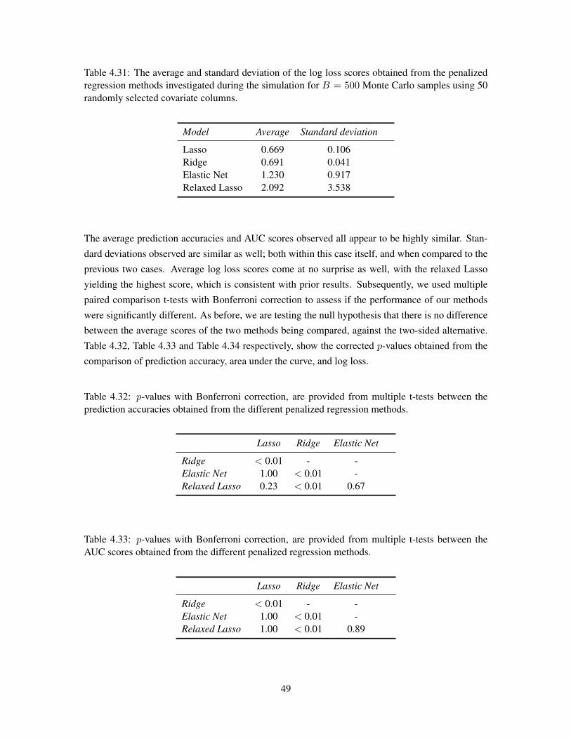
Table 4.31: The average and standard deviation of the log loss scores obtained from the penalizedregression methods investigated during the simulation for B = 500 Monte Carlo samples using 50randomly selected covariate columns.



The average prediction accuracies and AUC scores observed all appear to be highly similar. Stan-

dard deviations observed are similar as well; both within this case itself, and when compared to the

previous two cases. Average log loss scores come at no surprise as well, with the relaxed Lasso

yielding the highest score, which is consistent with prior results. Subsequently, we used multiple

paired comparison t-tests with Bonferroni correction to assess if the performance of our methods

were significantly different. As before, we are testing the null hypothesis that there is no difference

between the average scores of the two methods being compared, against the two-sided alternative.

Table 4.32, Table 4.33 and Table 4.34 respectively, show the corrected p-values obtained from the

comparison of prediction accuracy, area under the curve, and log loss.

Table 4.32: p-values with Bonferroni correction, are provided from multiple t-tests between theprediction accuracies obtained from the different penalized regression methods.


Ridge < 0.01 - -Elastic Net 1.00 < 0.01 -Relaxed Lasso 0.23 < 0.01 0.67

Table 4.33: p-values with Bonferroni correction, are provided from multiple t-tests between theAUC scores obtained from the different penalized regression methods.


Ridge < 0.01 - -Elastic Net 1.00 < 0.01 -Relaxed Lasso 1.00 < 0.01 0.89

49

Table 4.34: p-values with Bonferroni correction, are provided from multiple t-tests between the logloss scores obtained from the different penalized regression methods.


Ridge 1.00 - -Elastic Net < 0.01 < 0.01 -Relaxed Lasso < 0.01 < 0.01 < 0.01

50

4.5 Discussion of Results

Through our simulation study, we assessed the performance of the different regularization ap-

proaches investigated by looking at various evaluation metrics. We also examined the algorithmic

runtime taken for each of the different classification methods under the varying n, p conditions, as

well as post-selection approaches for obtaining p-values of coefficient estimates. In this section, we

provide a brief discussion of the results obtained, and why we might be observing some of these

results. However, due to the limited scope of our study, even though certain performance measures

obtained between the different fitting approaches were sometimes determined to be significantly

different, we are unable to truly say if any given method is better than another. Instead, we will

direct our focus towards identifying the weaknesses of each approach.

4.5.1 Evaluation Metrics

The evaluation metrics examined during our study were the prediction accuracy, logarithmic loss

and area under the curve of the resulting classifications made by our classifiers. Table 4.35 sum-

marizes the results we obtained from the simulation by showing the average scores of each of the

evaluation metrics, under the three different n, p conditions investigated.

Table 4.35: Summary of results obtained from each of the 3 different cases investigated during thesimulation. In Case 1., we had p > n, Case 2. p = n with the 50 highest correlated covariates, andin Case 3. we had p = n with 50 randomly chosen covariates.

Metric Lasso Ridge Elastic Net Relaxed Lasso

Case 1. Accuracy 0.710 0.682 0.714 0.705p > n Log Loss 0.611 0.628 1.600 3.107

AUC 0.778 0.751 0.749 0.720

Case 2. Accuracy 0.744 0.752 0.741 0.740p = n Log Loss 0.544 0.550 0.639 1.993

AUC 0.830 0.846 0.830 0.815

Case 3. Accuracy 0.606 0.541 0.610 0.626p = n Log Loss 0.669 0.691 1.230 2.092

AUC 0.680 0.631 0.668 0.684

51

We find that the scores obtained for our evaluation metrics in Case 2, where we had p = n using only

using the 50 covariates that had the highest correlation with the response, were significantly better

than the other 2 cases across the board. Case 1 appears to have performance that lies between Case

2 and Case 3, with Case 3 having the worst performance out of the three. Specifically in terms of the

log loss, we find that the Lasso always outperformed the other fitting approaches, regardless of n, p

conditions. Conversely, although its other performance measures are comparable to the remaining

fitting approaches, the relaxed Lasso always yielded the worst logarithmic loss score across the

board. This seems to suggest that although the relaxed Lasso performed well in terms of assigning

class labels, when it mis-classified, it often assigned a much higher probability to incorrect labels as

compared to all the other models.

4.5.2 Sparsity

Although briefly mentioned earlier in the paper, we have not really addressed the issue of the spar-

sity of our constructed models. An ideal model would be capable of yielding a desired level of

performance while using the least number of predictors possible. A sparse model has many ben-

efits, among which include are fact that it is easier to interpret, as well as being computationally

lighter. Table 4.36 shows the average number of non-zero coefficients retained by each of the pe-

nalized regression models during the simulation study.

Table 4.36: The number of covariates selected by the Lasso and elastic net regularizations under thethree different n, p conditions.

Lasso Elastic Net

Case 1.(p > n

)12 77

Case 2.(p = n

)7 13

Case 3.(p = n

)5 14

Notice we avoided showing the results for the ridge and relaxed Lasso models, since the former

does not perform variable selection and the latter naturally selects the same variables as the Lasso.

From the results obtained, we observed that the Lasso enjoyed greater sparsity than the elastic net

across all three n, p cases when tuning parameters were chosen through 10-fold cross validation,

while retaining a similar level of performance. We point out that this is exactly the opposite of

what Zou and Hastie have stated, where the elastic net was supposed to outperform the Lasso while

retaining a similar level of sparsity [23]. One might naturally suspect that this has to do with the

choice of values for tuning parameters. However, although specific methods of selecting values

for tuning parameters were not proposed by Zou and Hastie, they do suggest that 10-fold cross

validation is an extremely viable choice.

52

4.5.3 Multi Sample-Splitting

From the results obtained from our simulation study, we observed that Buhlmann et. al.’s multi

sample-splitting method did not detect significance in most of the coefficients retained by the elastic

net models fitted under the varying n, p conditions. However, we know that this should not be

the case, since we had simulated our data based on the true covariates of 1278 and 4003. As

such, one might naturally stipulate that a well-performing algorithm would be capable of detecting

significance in those two covariates. To investigate why we failed to detect significance in practically

all of the coefficients obtained from the elastic net during the simulation study, we decided to apply

the multi sample splitting method on the Lasso as well. The results obtained were similar to that

of the elastic net - where we failed to detect significance in most of the coefficients. In turn, this

provided a stark construct with that of the covariance test, which frequently managed to detect

the active variables of 1278 and 4003. However, the covariance test also frequently determined

covariates other than 1278 and 4003 to be significant as well.

However, what we noticed was that during the p-value estimation process based on standard

least squares (Step 3. of Algorithm 1.), standard errors of the coefficients generated from the linear

model were highly inflated, suggesting the presence of multi-collinearity. Upon investigating, we

found that the covariates retained in the model were often moderately to highly correlated with each

other. Since individual standard errors were inflated, the p-values we obtained were naturally almost

always insignificant. As such, this offers an explanation as to why the multi sample-splitting method

did not yield the expected results. Another possible explanation might be that the approach we took

to choosing our tuning parameters, 10-fold cross validation, is ill-suited for the problem at hand. Of

course, none of these necessarily indicate that the method itself is inherently flawed, but rather the

fact that it might be a poor choice due to the nature of the riboflavin dataset.

We recognize that one of the main advantages of the sample splitting method is its flexibility to

accommodate different modeling or fitting approaches of choice, and obtain p-values for coefficient

estimates obtained from any of those approaches [15]. However, due to the fact that the sample

splitting method is generalized in a sense - that is to say, it is not specifically tailored to handle a

particular modeling or fitting approach, we naturally suspect that its performance may not be up to

par when compared to tailored approaches. This was the primary reason why we initially chose to

utilize the covariance test for the Lasso while employing the sample splitting method for the elastic

net during our simulation study, since there currently does not exist any method specifically devised

for obtaining p-values of elastic net coefficients.

We point out the short-comings of the method which causes it to perform poorly when multi-

collinearity is present. Consider this. Suppose that we fit the standard linear model to the riboflavin

dataset using only 3 covariates - 1278, 1279 and 4003. In Figure 4.3, we show the correlation

structure. If we fit the linear model with all 3 covariates, we in fact determine that both 1278 and

1279 are not significant. Conversely, if we fitted the model with only either of 1278 or 1279, we

would determine that they were in fact significant, along with 4003. Due to the fact 1278 and 1279

53

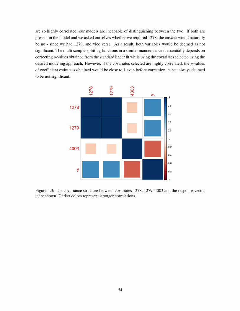
are so highly correlated, our models are incapable of distinguishing between the two. If both are

present in the model and we asked ourselves whether we required 1278, the answer would naturally

be no - since we had 1279, and vice versa. As a result, both variables would be deemed as not

significant. The multi sample-splitting functions in a similar manner, since it essentially depends on

correcting p-values obtained from the standard linear fit while using the covariates selected using the

desired modeling approach. However, if the covariates selected are highly correlated, the p-values

of coefficient estimates obtained would be close to 1 even before correction, hence always deemed

to be not significant.

Figure 4.3: The covariance structure between covariates 1278, 1279, 4003 and the response vectory are shown. Darker colors represent stronger correlations.

54


In Section 4.2, we investigated whether the order in which covariates entered the Lasso was related

to statistical significance. We found that when either of the two active variables were the first to

enter the model, they were often determined to be significant across the varying n, p cases. How-

ever, when they were the second to enter the model, they were essentially never determined to be

significant. Yet, when they entered the model third or later, they were frequently determined to be

significant again (Table 4.19). As a result, we observe an interesting cyclic behavior of the relation-

ship between the knot k at which a coefficient enters the Lasso model, and the significance of that

particular coefficient when judged by the covariance test.

We recall that under the null hypothesis of no active variables, T1 and T2 are asymptotically

independent exponential. This hypothesis is false in our covariance test but Figure 4.4 shows some

signs of T1 and T2 having little correlation. Lockhart et. al. [10] contains only a very incomplete

discussion of the logistic regression case, so the following discussion considers only the use of the

covariance test in the linear model. We suspect that the logistic regression case will be analogous.

Provided that we are at step k = 1 and X has unit norm columns, the covariance test statistic

can be simplified to T1 = λ1(λ1 − λ2)/σ2. By further assuming that X satisfies the positive cone

condition, one can generalize the previous simplification to Tk = λk(λk − λk+1)/σ2. We direct

our readers to Lockhart et. al.’s paper [10] where a comprehensive discussion and justification are

provided. Now, notice that in order for any given coefficient entering the Lasso model at knot k to

be significant, Tk has to be large - which happens to be the case when λk is large and λk+1 is small.

That is to say, the first coefficient to enter the model is likely to significant when when λ1 is large

and λ2 is small, since T1 would be large. However, this implies that T2 = λ2(λ2 − λ3)/σ2 is likely

to be small because λ2 is small, and hence the second coefficient to enter the Lasso model is likely

to determined not significant by the covariance test.

We believed this to be a possible explanation for the cyclic behavior we were observing in

Section 4.2, and as such, investigated if this was truly the case. To do so, we plotted the covariance

test statistics of the first and second coefficients to enter the Lasso model (T1 and T2) obtained across

the B = 100 iterations, against each other in Figure 4.4. There did not appear to be a strong linear

relationship between T1 and T2 (with ρ = -0.22), and instead we notice something that resembles an

exponential decay. In particular, this relationship observed is supportive of our proposed explanation

for the cyclic pattern of variable significance, where a larger value of T1 corresponds to a smaller

value of T2. Although we are unable to assert this with certainty, it definitely offers a plausible

explanation for the results obtained from our simulation study.

55

Figure 4.4: The covariance test statistics T1 and T2 for the first and second coefficients to enter themodel along the Lasso solution path, across the B = 100 iterations of the simulation, are plottedagainst each other.

4.5.5 Algorithm Runtime

Here, we are interested in the runtime of the different modeling and post selection algorithms in

consideration. We used the glmnet package in R, for the Lasso, elastic net and ridge regression

methods. This package uses coordinate descent to obtain coefficient estimates. We direct readers to

Friedman et. al. [6] for a comprehensive discussion behind the theory and time complexity of the

coordinate descent algorithm. Table 4.37 shows the average runtimes for each of the different fitting

approaches, across the iterations of our simulation study. Since the size of n and p remain the same

between Case 2 (n = p with 50 highest correlation) and Case 3 (n = p with 50 randomly selected),

we do not bother keeping track of the runtime separately for these two cases; there is likely to be

a negligible difference. All computations were performed on a machine with an Intel i7-6700K @

4.00GHz processor, with 16.0 GB RAM and a NVIDIA GTX 1070 grahics card.

Table 4.37: Algorithm runtimes (seconds) are provided for each of the different fitting approachesemployed under different n, p conditions.


p > n 0.393 3.304 4.240 0.398p = n 0.103 0.083 1.495 0.106

56

We observe that the elastic net consistently required the longest runtime in both the cases where

p = n and p > n, which can be attributed to the fact that the elastic net requires tuning of 2

parameters as opposed to the single one in the cases of the Lasso and ridge. The relaxed Lasso

always required a longer runtime than the Lasso, since it involves fitting the Lasso model first in

order to select the subset with which to fit the standard linear model. Hence the difference between

the 2 runtimes is solely attributed to the small time taken to fit the standard linear model. We also

note that although the ridge penalty resulted in an approximate 8 times longer runtime than the Lasso

in the case where p > n, when we shifted to the case of p = n, the ridge penalty ended up yielding

the shortest runtime out of all the methods in consideration. However, it was not determined to be

significantly different from either the Lasso or relaxed Lasso.

Based on our simulation study alone, we are unable to provide an appropriate comparison be-

tween the runtimes of the multi sample-splitting method and the covariance test due to the fact that

one was applied on the Lasso coefficients, while the other on the elastic net. We note that one of the

main advantages of the covariance test is its capability of determining significance for coefficient

estimates in a sequential manner - that is to say, we can choose to simply assess the first two coeffi-

cients that entered the Lasso model, instead of all selected coefficients. Conversely, this is not true

for the multi sample splitting method, which requires all selected variables to be included together,

hence creating an all-or-nothing situation. As such, in order to facilitate a valid comparison, we ap-

plied both the covariance test and the multi sample splitting method on the Lasso model, reran our

simulation, and assessed the significance of all coefficients selected. Table 4.38 shows the average

runtime of the two algorithms, under the cases where p > n and p = n.

Table 4.38: Average runtimes (seconds) are provided for each of the different approaches employedunder different n, p conditions for obtaining p-values for Lasso coefficient estimates.

Covariance Test Multi Sample-Splitting

p > n 6.652 14.823p = n 0.682 5.703

We observe that the covariance test has a significantly shorter runtime than the multi sample-splitting

method in both cases. Coupled with the fact that the covariance test performs much better in the

presence of correlated covariates, we believe that the covariance test is the better approach of choice

when assessing the significance of Lasso coefficient estimates.

4.5.6 How much are we losing from dichotomizing?

Recall that the response variable for the riboflavin dataset - the log-transformed riboflavin produc-

tion rate, is in fact initially a continuous variable. For our purposes, we chose to dichotomize it such

that it becomes applicable in the context of logistic regression. As a result, this begs the question,

57

how much information are we losing by doing so? In particular, of interest is the difference in predic-

tion accuracies that might happen to be observed. Intuitively, we suspect that post-dichotomization

would result in a higher prediction accuracy than that of pre-dichotomization. To investigate this,

we process the dataset and build our models through 2 different streams. The first is the procedure

which we have been following thus far − we dichotomize the response variable before fitting our

logistic regression model to the data, and subsequently make predictions on the test set and eval-

uate them against the true values. Subsequently, we will call this pre-dichotomization from now

onwards.

Conversely, in the second stream, we do not dichotomize the response variable initially, and

instead fit the standard linear regression model to the data. We then proceed to make predictions

on the test set based on the linear model, and only after which would we proceed to dichotomize

the predictions in the same manner as we had done for the response variable, and finally validate

the results against the true values. This then becomes what we call post-dichotomization. In order

to compare the 2 different steams, we perform paired t-tests to assess if the difference between the

average prediction accuracies from pre-dichotomization and post-dichotomization are significantly

different. We denote this difference by δ. As such, we are in fact testing the null hypothesis and its

two-sided alternative of:

H0 : δ = 0

HA : δ 6= 0(4.3)

Tables 4.39, 4.40 and 4.41 contain pre- and post-dichotomization prediction accuracies for each

of the four different classification approaches for the three cases of p > n, p = n with highly

correlated covariates, and p = n with randomly selected covariates, respectively. We are unable to

derive the log loss and area under the curve in this case, since post-dichotomization revolves around

fitting a linear regression model, which is not a classifier, and hence does not provide prediction

probabilities.

Table 4.39: Pre- and post-dichotomized average prediction accuracies and standard deviations inthe case where p > n for each of the four classification methods investigated during the simulation.A total of B = 100 Monte Carlo samples are run. The p-values are from a two-sided pairedcomparison t-test of the hypothesis that there is no difference between the classification methods.Significance at α levels of 0.05, 0.01, 0.001 is denoted by the varying number of asterisks (∗).

Model Pre-Dichotomized (SD) Post-Dichotomized (SD) Difference (δ) p-value

Lasso 0.710 (0.115) 0.766 (0.092) 0.056 < 0.01 ∗∗

Ridge 0.682 (0.119) 0.705 (0.115) 0.023 0.045 ∗

Elastic Net 0.714 (0.105) 0.719 (0.108) 0.005 0.752Relaxed Lasso 0.705 (0.101) 0.713 (0.103) 0.008 0.593

58

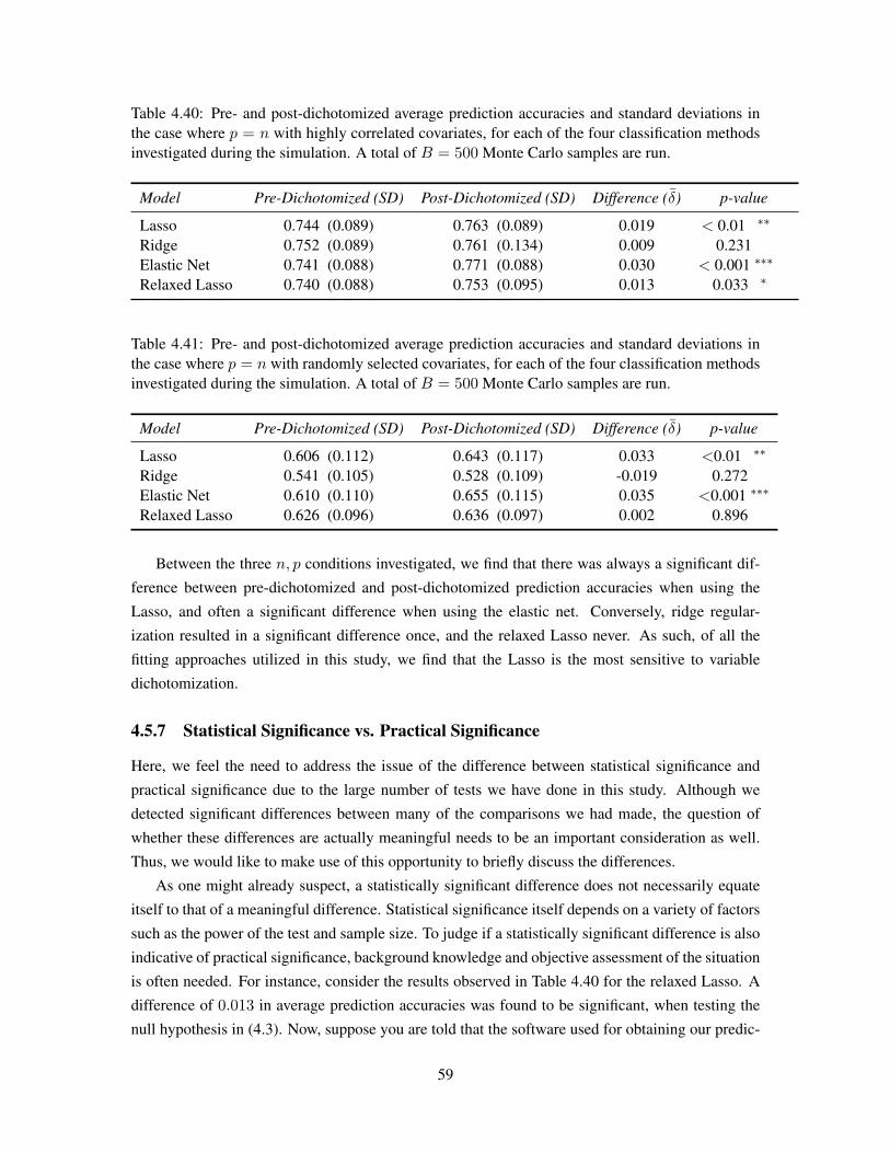
Table 4.40: Pre- and post-dichotomized average prediction accuracies and standard deviations inthe case where p = n with highly correlated covariates, for each of the four classification methodsinvestigated during the simulation. A total of B = 500 Monte Carlo samples are run.


Lasso 0.744 (0.089) 0.763 (0.089) 0.019 < 0.01 ∗∗

Ridge 0.752 (0.089) 0.761 (0.134) 0.009 0.231Elastic Net 0.741 (0.088) 0.771 (0.088) 0.030 < 0.001 ∗∗∗

Relaxed Lasso 0.740 (0.088) 0.753 (0.095) 0.013 0.033 ∗

Table 4.41: Pre- and post-dichotomized average prediction accuracies and standard deviations inthe case where p = n with randomly selected covariates, for each of the four classification methodsinvestigated during the simulation. A total of B = 500 Monte Carlo samples are run.


Lasso 0.606 (0.112) 0.643 (0.117) 0.033 <0.01 ∗∗

Ridge 0.541 (0.105) 0.528 (0.109) -0.019 0.272Elastic Net 0.610 (0.110) 0.655 (0.115) 0.035 <0.001 ∗∗∗

Relaxed Lasso 0.626 (0.096) 0.636 (0.097) 0.002 0.896

Between the three n, p conditions investigated, we find that there was always a significant dif-

ference between pre-dichotomized and post-dichotomized prediction accuracies when using the

Lasso, and often a significant difference when using the elastic net. Conversely, ridge regular-

ization resulted in a significant difference once, and the relaxed Lasso never. As such, of all the

fitting approaches utilized in this study, we find that the Lasso is the most sensitive to variable

dichotomization.

4.5.7 Statistical Significance vs. Practical Significance

Here, we feel the need to address the issue of the difference between statistical significance and

practical significance due to the large number of tests we have done in this study. Although we

detected significant differences between many of the comparisons we had made, the question of

whether these differences are actually meaningful needs to be an important consideration as well.

Thus, we would like to make use of this opportunity to briefly discuss the differences.

As one might already suspect, a statistically significant difference does not necessarily equate

itself to that of a meaningful difference. Statistical significance itself depends on a variety of factors

such as the power of the test and sample size. To judge if a statistically significant difference is also

indicative of practical significance, background knowledge and objective assessment of the situation

is often needed. For instance, consider the results observed in Table 4.40 for the relaxed Lasso. A

difference of 0.013 in average prediction accuracies was found to be significant, when testing the

null hypothesis in (4.3). Now, suppose you are told that the software used for obtaining our predic-

59

tion accuracies is somehow flawed, and may randomly deviate from the actual prediction accuracies

by a margin of 0.10. As such, although we detect statistical significance, it is unlikely to be practi-

cally significant, since our observed difference might easily be caused by random fluctuations. We

also note that if we were to increase the sample size from 500 to some extremely large value, one

might even be able to detect statistical significance in a difference of 0.00013. One would then have

to ask themselves whether a tenth of a percentage point has any real practical benefits. External

factors often play an important role in determining if statistical significance is actually practical.

One might consider other approaches, such as constructing confidence intervals, to aid in making

an appropriate decision.

60

Chapter 5

Conclusion

In this paper, we investigated common regularization approaches for fitting logistic regression mod-

els with binary response variables in a high-dimensional setting. Through our simulation study,

we were able to identify weaknesses of certain fitting approaches. We found that the elastic net

model often selected a larger number of non-zero coefficients and required a longer computation

time when compared to the Lasso, while retaining a similar level of performance when judged by

our evaluation metrics. This is contrary to what Zou and Hastie have suggested [23], where the

elastic net was supposed to enjoy a similar level of sparsity while maintaining comparable model

performance. We also find that the multi sample-splitting method proposed by Buhlmann et. al.

performs poorly when coefficients selected by our models happen to be correlated with each other.

However, Lockhart et al’s covariance test did not suffer from this issue, and was computationally

faster. It did, however, find statistical significance of inactive variables fairly often.

5.1 Extensions and Future Work

Due to time constraints, there were many issues and aspects that we considered, but were unable

to follow-up with further investigation. The concept of logistic regression is inherently broad, and

even with the limited scope that we have worked in this paper, we leave a lot open for future work.

For instance, although we provided possible explanations, we did not manage to precisely determine

why exactly we were observing a cyclic behavior from the significance of Lasso coefficients when

judged by the covariance test. We also considered only the Lasso, ridge, elastic net and relaxed

Lasso regularization approaches, which were chosen due to the fact that they are widely used, but

there are many other existing approaches which we have not yet investigated. For instance, Mein-

shausen et. al. [15] provides discussions on the applications of the multi sample splitting method

to the adaptive Lasso [22], which was an avenue which we could have investigated and compared

with our present methods.

61

We also recognize the limitations of our study - where we only used two different datasets, and

both with relatively small sample sizes. Additionally, we note that the logistic model is wrong for

our simulated data, since our error terms were generated from a Gaussian distribution. Furthermore,

since we inherently reject the null under the premise of the setup of our simulation study, we find

ourselves lacking a calibration study to evaluate the behavior of the covariance test where our null

hypothesis is true. Looking back, we have also considered simply simulating a new set of data

points to utilize as a test set, instead of splitting our original dataset into separate smaller training

and test sets; this would have proved advantageous by increasing the sample sizes allocated for both

training and validation. If provided with more time - the simulation study could have been run for a

larger number of Monte Carlo samples, properties of our models could have been explored in greater

detail, and additional performance evaluations could have been used to asses our models. Methods

for deriving confidence intervals for coefficient estimates could have been explored as well. It is

regrettable that we are unable to cover all of these issues, but if presented with the opportunity, we

will definitely seek to address them in future work.

62

Bibliography

[1] Kaggle past solutions. https://www.kaggle.com/wiki/PastSolutions. Ac-cessed: 2017-02-10.

[2] Peter Bühlmann, Markus Kalisch, and Lukas Meier. High-dimensional statistics with a viewtoward applications in biology. Annual Review of Statistics and Its Application, 1:255–278,2014.

[3] Peter Bühlmann and Jacopo Mandozzi. High-dimensional variable screening and bias in sub-sequent inference, with an empirical comparison. Computational Statistics, 29(3-4):407–430,2014.

[4] Ruben Dezeure, Peter Bühlmann, Lukas Meier, and Nicolai Meinshausen. High-dimensionalinference: Confidence intervals, p-values and R-software hdi. Statistical Science, 30(4):533–558, 2015.

[5] Kevin K Dobbin and Richard M Simon. Optimally splitting cases for training and testing highdimensional classifiers. BMC medical genomics, 4(1):31, 2011.

[6] Jerome Friedman, Trevor Hastie, and Rob Tibshirani. Regularization paths for generalizedlinear models via coordinate descent. Journal of statistical software, 33(1):1, 2010.

[7] Arthur Hoerl and Robert Kennard. Ridge regression: Biased estimation for nonorthogonal problems. Technometrics, 12(1):55–67, 1970.

[8] Max Kuhn. Contributions from Jed Wing, Steve Weston, Andre Williams, Chris Keefer, AllanEngelhardt, Tony Cooper, Zachary Mayer, Brenton Kenkel, the R Core Team, Michael Ben-esty, Reynald Lescarbeau, Andrew Ziem, Luca Scrucca, Yuan Tang, Can Candan, and Tyler Hunt. caret: Classification and regression training, 2016. R package version 6.0-73

[9] Richard Lockhart, Jonathan Taylor, Ryan J Tibshirani, and Robert Tibshirani. A significancetest for the lasso. Annals of statistics, 42(2):413, 2014.

[10] Vivien Marx. Biology: The big challenges of big data. Nature, 498(7453):255–260, 2013.

[11] John A Nelder and Robert Wedderburn. Generalized linear models. Journal of the Royal StatisticalSociety. Series A (General), 135(3), 370-384, 1972.

[12] Nicolai Meinshausen. Relaxed lasso. Computational Statistics & Data Analysis, 52(1):374–393, 2007.

63

https://www.kaggle.com/wiki/PastSolutions

[13] Nicolai Meinshausen and Peter Bühlmann. Stability selection. Journal of the Royal StatisticalSociety: Series B (Statistical Methodology), 72(4):417–473, 2010.

[14] Nicolai Meinshausen, Lukas Meier, and Peter Bühlmann. P-values for high-dimensional re-gression. Journal of the American Statistical Association, 104(488):1671–1681, 2009.

[15] R Core Team. R: A language and environment for statistical computing, 2016.

[16] Robert Tibshirani. Regression shrinkage and selection via the lasso. Journal of the RoyalStatistical Society. Series B (Methodological), pages 267–288, 1996.

[18] Ryan Joseph Tibshirani, Jonathan E Taylor, Emmanuel Jean Candes, and Trevor Hastie. Thesolution path of the generalized lasso. 2011.

[19] W. N. Venables and B. D. Ripley. Modern applied statistics with s. 2002. ISBN 0-387-95457-0.

[20] Stijn Viaene, Mercedes Ayuso, Montserrat Guillen, Dirk Van Gheel, and Guido Dedene.Strategies for detecting fraudulent claims in the automobile insurance industry. EuropeanJournal of Operational Research, 176(1):565–583, 2007.

[21] Larry Wasserman and Kathryn Roeder. High dimensional variable selection. Annals of statis-tics, 37(5A):2178, 2009.

[22] Hui Zou. The adaptive lasso and its oracle properties. Journal of the American statisticalassociation, 101(476):1418–1429, 2006.

[23] Hui Zou and Trevor Hastie. Regularization and variable selection via the elastic net. Journalof the Royal Statistical Society: Series B (Statistical Methodology), 67(2):301–320, 2005.

64

[17] Robert Tibshirani. Jerome Friedman, Trevor Hastie. glmnet: Regularization paths for general-ized linear models via coordinate descent, 2010. R package version 6.0-73.

Appendix A

Code

R code used for the simulation study is compiled using R Markdown and is attached on the nextpage.

65

Code for Simulation Study#Clear working enviroment.rm(list = ls())

#Set random seed.set.seed(13337)

#Load packages and data.

library(hdi)

## Loading required package: scalreg

## Loading required package: lars

## Loaded lars 1.2

## Loading required package: MASSlibrary(glmnet)

## Loading required package: Matrix

## Loading required package: foreach

## Loaded glmnet 2.0-5library(MLmetrics)

#### Attaching package: 'MLmetrics'

## The following object is masked from 'package:base':#### Recalllibrary(ggplot2)library(corrplot)library(covTest)

## Loading required package: glmpath

## Loading required package: survivaldata("riboflavin")

#Main function for running our simulation, modelling and data manipulation are wrapped#inside. In particular, we look at the Lasso, Ridge, Elastic Net and Relaxed Lasso.

simulation = function(B = 100, case = 1){# This function runs the desired simluation as described in Section 4.1.## Args:# B: Interger specifying number of iterations to be run.## case: One of {1,2,3}. Specifies type of simulation to run, corresponding# to the cases presented in the paper.# 1. p > n# 2. p = n with 50 top correlated covariates# 3. p = n with random selected covariates

66

## Returns:# M1 - M4: Matrices M1, M2, M3, M4 contain coefficient estimates obtained from each of# the four different fitting methods investigated.## P1 - P4: Matrices P1, P2, P3, P4 contain prediction accuracies obtained from each# of the the four different fitting methods investigated.## A1 - A4: Matrices A1, A2, A3, A4 contain area under the curve scores obtained from# each of the four different fitting methods investigated.## L1 - L4: Matrices L1, L2, L3, L4 contain logarithmic loss scores obtained from# each of the four different fitting methods investigated.### Details:# The simulation itself entails creating a fake 'pseudo' dataset based on the# riboflavin dataset in the hdi package. Each simulated dataset is created with# the same design matrix X and the same two betas (the first two to enter the Lasso ).# The variance of epsilon, sigma^2, is estimated with RSS/n.# Epsilon is then generated from a normal distribution with mean 0 and variance sigma^2.# Distinct beta's are used for each of lasso, elastic net, ridge and the elastic net.##-----------------------------------------------------------------------------------------#

#Centering and standarding the riboflavin data.x <- as.vector(riboflavin$x)x <- scale(matrix(x, 71, 4088), T, T)y <- as.vector(scale(riboflavin$y, center = T))

if((case %in% c(1,2,3)) == F){stop("case has to take values in {1, 2, 3}")

}else{if(case == 1){

df <- data.frame(x = x, y = y)}if(case == 2){

ip <- sample(1:4088, 50, replace = F)x <- x[ , ip]df <- data.frame(x = x, y = y)colnames(df) <- c(as.character(ip), "y")

}if(case == 3){

ip <- order(abs(cor(x,y)), decreasing = T)[1:50]x <- x[ , ip]df <- data.frame(x = x, y = y)colnames(df) <- c(as.character(ip), "y")

}}

#------------------------------------------------------------------------------------------## Fit preliminary lasso, and select only the first 2 covariates to enter the model.#------------------------------------------------------------------------------------------#

67

lvar <- ncol(df)splitval <- mean(df$y)cv_fit <- cv.glmnet(x = as.matrix(df[, -lvar]), y = as.vector(df$y),

family = "gaussian", alpha = 1)lasso_fit <- glmnet(x = as.matrix(df[, -lvar]), y = as.vector(df$y), family = "gaussian",

alpha = 1, lambda = cv_fit$lambda[which(cv_fit$nzero > 1)[1]])nzero_ind <- which(lasso_fit$beta!=0)lm_fit <- lm(y~., data = df[, nzero_ind])

beta_two <- as.vector(lm_fit$coefficients)rss <- sum((as.vector(df$y) - predict(lm_fit, newdata = df[, -lvar]))^2)sigma_hat <- rss/71zerovec <- rep(0, (lvar-1))zerovec[nzero_ind] <- beta_two[2:length(beta_two)]xbeta <- as.matrix(df[, -lvar])%*%c(as.vector(zerovec))

#------------------------------------------------------------------------------------------## Generate matrices/lists to store results.#------------------------------------------------------------------------------------------#

P1 <- P2 <- P3 <- P4 <- matrix(NA, B, 2) #Store prediction accuracies, pre- & post-dichotomized.M1 <- M2 <- M3 <- M4 <- matrix(NA, (lvar-1), B) #Store coefficient values for pre- only.L <- matrix(NA, B, 4) #Store log loss scores for pre- only.A <- matrix(NA, B, 4) #Store area under the curve scores for pre- only.

#------------------------------------------------------------------------------------------## Run Monte Carlo#------------------------------------------------------------------------------------------#

for(i in 1:B){

#Generate pseudo data for every iteration by sampling new values for epsilonycont <- xbeta + rnorm(71, mean = 0, sd = sqrt(sigma_hat))ybin <- ycontybin[which(ybin > splitval)] <- 1ybin[which(ybin != 1)] <- 0pseudo_df <- data.frame(x, y = ybin)

#Sample splittings <- sample(1:71, 50)train <- pseudo_df[s, ]test <- pseudo_df[-s, ]

#Lassofit1_cv <- cv.glmnet(x = as.matrix(train[, -lvar]), y = as.factor(train$y),

family = "binomial", alpha = 1)fit1 <- glmnet(x = as.matrix(train[, -lvar]), y = as.factor(train$y),

family = "binomial", alpha = 1, lambda = fit1_cv$lambda.min)M1[, i] <- as.vector(fit1$beta)p1 <- predict(fit1, newx = as.matrix(test[, -lvar]), type = "response")p1_acc <- sum(round(p1) == test$y)/nrow(test)P1[i, 1] <- p1_accL[i, 1] <- LogLoss(predict(fit1, newx = as.matrix(test[, -lvar]), type = "response"), test$y)A[i, 1] <- AUC(predict(fit1, newx = as.matrix(test[, -lvar]), type = "response"), test$y)

#Ridge

68

fit2_cv <- cv.glmnet(x = as.matrix(train[, -lvar]), y = as.factor(train$y),family = "binomial", alpha = 0)

fit2 <- glmnet(x = as.matrix(train[, -lvar]), y = as.factor(train$y),family = "binomial", alpha = 0, lambda = fit2_cv$lambda.min)

M2[, i] <- as.vector(fit2$beta)p2 <- predict(fit2, newx = as.matrix(test[, -lvar]), type = "response")p2_acc <- sum(round(p2) == ybin[-s])/nrow(test)P2[i, 1] <- p2_accA[i, 2] <- AUC(predict(fit2, newx = as.matrix(test[, -lvar]), type = "response"), test$y)L[i, 2] <- LogLoss(predict(fit2, newx = as.matrix(test[, -lvar]), type = "response"), test$y)

#Elastic Netfit3_cv <- train(x = as.matrix(train[, -lvar]), y = as.factor(train$y),

method ="glmnet", family = "binomial")fit3 <- glmnet(x = as.matrix(train[, -lvar]), y = as.factor(train$y), family = "binomial",

alpha = fit3_cv$bestTune[1], lambda = fit3_cv$bestTune[2])M3[, i] <- as.vector(fit3$beta)p3 <- predict(fit3, newx = as.matrix(test[, -lvar]), type = "response")p3_acc <- sum(round(p3) == ybin[-s])/nrow(test)M3[i, 1] <- p3_accA[i, 3] <- AUC(predict(fit3, newx = as.matrix(test[, -lvar]), type = "response"), test$y)L[i, 3] <- LogLoss(predict(fit3, newx = as.matrix(test[, -lvar]), type = "response"), test$y)

#Relaxed Lassorelax_ind <- which(as.vector(fit1$beta) != 0 )relax_df <- train[, c(relax_ind, lvar)]lm_fit <- glm(y~. , data = relax_df, family = binomial)p4 <- predict(lm_fit, (test[, -lvar]), type = "response")p4_acc <- sum(round(p4) == test$y)/nrow(test)P4[i, 1] <- p4_accL[i, 4] <- LogLoss(predict(lm_fit, (test[, -lvar]), type = "response"), test$y)A[i, 4] <- AUC(predict(lm_fit, (test[, -lvar]), type = "response"), test$y)

#---------------------------------------------------------------------------------------------------------------------## WITHOUT Dichotomization#---------------------------------------------------------------------------------------------------------------------#

#Sample splittingpseudo_df2 <- data.frame(x = x, y = ycont)train <- pseudo_df2[s, ]test <- pseudo_df2[-s, ]

#Lassofit1_cv <- cv.glmnet(x = as.matrix(train[, -lvar]), y = as.vector(train$y),

family = "gaussian", alpha = 1)fit1 <- glmnet(x = as.matrix(train[, -lvar]), y = as.vector(train$y),

family = "gaussian", alpha = 1, lambda = fit1_cv$lambda.min)p1 <- predict(fit1, newx = as.matrix(test[, -lvar]), type = "response")p1[which(p1 > splitval)] <- 1p1[which(p1 != 1)] <- 0p1_acc <- sum(p1 == ybin[-s])/nrow(test)P1[i, 2] <- p1_acc

#Ridge

69

fit2_cv <- cv.glmnet(x = as.matrix(train[, -lvar]), y = as.vector(train$y),family = "gaussian", alpha = 0)

fit2 <- glmnet(x = as.matrix(train[, -lvar]), y = as.vector(train$y),family = "gaussian", alpha = 0, lambda = fit2_cv$lambda.min)

p2 <- predict(fit2, newx = as.matrix(test[, -lvar]), type = "response")p2[which(p2 > splitval)] <- 1p2[which(p2 != 1)] <- 0p2_acc <- sum(round(p2) == ybin[-s])/nrow(test)P2[i, 2] <- p2_acc

#Elastic Netfit3_cv <- train(x = as.matrix(train[, -lvar]), y = train$y, method ="glmnet", family = "gaussian")fit3 <- glmnet(x = as.matrix(train[, -lvar]), y = train$y, alpha = fit3_cv$bestTune[1],

lambda = fit3_cv$bestTune[2])p3 <- predict(fit3, newx = as.matrix(test[, -lvar]), type = "response")p3[which(p3 > splitval)] <- 1p3[which(p3 != 1)] <- 0p3_acc <- sum(p3 == ybin[-s])/nrow(test)P3[i, 2] <- p3_acc

#Relaxed Lassorelax_ind <- which(as.vector(fit1$beta) != 0 )relax_df <- train[, c(relax_ind, lvar)]lm_fit <- lm(y~., data = relax_df)p4 <- predict(lm_fit, (test[, -lvar]), type = "response")p4[which(p4 > splitval)] <- 1p4[which(p4 != 1)] <- 0p4_acc <- sum(p4 == ybin[-s])/nrow(test)P4[i, 2] <- p4_acc

#Keep track of current iterationprint(paste("Iteration", as.character(i), " is done."))

}return(list(M1, M2, M3, M4, P1, P2, P3, P4, L, A))

}

70

Appendix B

List of randomly selected covariatesused in Case 3.

R code used is compiled using R Markdown and is attached on the next page.

71

Covariates selected for Case 3.set.seed(13337)library(hdi)

## Loading required package: scalreg

## Loading required package: lars

## Loaded lars 1.2

## Loading required package: MASSdata("riboflavin")x <- as.vector(riboflavin$x)x <- scale(matrix(x, 71, 4088), center = T, scale = T)y <- as.vector(scale(riboflavin$y, center = T, scale = FALSE))r <- sample(1:4088, 50, replace = F)print(r)

## [1] 434 689 3244 2536 2733 573 2000 247 1864 3591 2030 195 3844 2596## [15] 1288 2573 3464 183 3842 1344 1186 2446 3290 3727 1135 461 1369 1349## [29] 3734 888 3746 1882 1338 3456 841 3048 1761 1147 2181 3994 1685 2624## [43] 179 2156 1281 1495 3668 2142 416 878

72

An Applied Analysis of High-Dimensional Logistic Regressionsummit.sfu.ca/system/files/iritems1/17392/etd10164_DQiu.pdf · An Applied Analysis of High-Dimensional Logistic Regression

Documents