An analytical model to predict regional groundwater discharge patterns on the floodplains of a semi-arid lowland river

An Analytical Model to Predict Regional Groundwater Discharge Patterns on the Floodplains of a Semi-Arid Lowland River Kate Holland, Ian Overton, Ian Jolly and Glen Walker

CSIRO Land and Water Technical Report No. 6/04 February 2004

© 2004 CSIRO To the extent permitted by law, all rights are reserved and no part of this publication covered by copyright may be reproduced or copied in any form or by any means except with the written permission of CSIRO Land and Water.

Important Disclaimer

CSIRO Land and Water advises that the information contained in this publication comprises general statements based on scientific research. The reader is advised and needs to be aware that such information may be incomplete or unable to be used in any specific situation. No reliance or actions must therefore be made on that information without seeking prior expert professional, scientific and technical advice.

To the extent permitted by law, CSIRO Land and Water (including its employees and consultants) excludes all liability to any person for any consequences, including but not limited to all losses, damages, costs, expenses and any other compensation, arising directly or indirectly from using this publication (in part or in whole) and any information or material contained in it.

ISSN 1446-6171

Cover Photograph

Clarks seepage lagoon on the River Murray floodplain near Bookpurnong in the South Australian Riverland

An Analytical Model to Predict Regional Groundwater Discharge Patterns on the Floodplains of a Semi-Arid Lowland River.

Kate Holland12, Ian Overton1, Ian Jolly1 and Glen Walker1

1CSIRO Land and Water, Urrbrae, Australia 2Flinders University of South Australia, Australia

CSIRO Land and Water Technical Report 6/04, February 2004

ACKNOWLEDGEMENTS

The first author was supported by an Australian Postgraduate Award scholarship and Centre for Groundwater Studies bursary at the time of the project, under the supervision of Glen Walker, Steve Tyerman, Craig Simmons, Lisa Mensforth and Andrew Telfer. Land and Water Australia (Project CWS8 – Guidelines for Managing Groundwater for Vegetation Health in Saline Areas) and the River Murray Catchment Water Management Board provided funding towards this project. Craig Simmons, Neville Robinson and Anthony Barr provided useful suggestions and comments that improved this report.

EXECUTIVE SUMMARY

River regulation, and both irrigated and dryland agricultural developments have increased saline groundwater discharge to the lower River Murray in south eastern Australia, affecting both river salinity and the floodplain environment. Part I of this report describes the development and testing of a simple, one dimensional analytical model that distributes floodplain groundwater discharge as seepage at the break of slope, evapotranspiration across the floodplain and as groundwater flow into and out of the river. The analytical model estimates were comparable to MODFLOW estimates (R2 = 0.998) over a broad range of typical floodplain recharge and evapotranspiration scenarios. Part II of report applies the model using regional scale GIS data to the lower River Murray, south eastern Australia. The model is able to predict groundwater discharge patterns within the floodplain. Using current groundwater inflow estimates, the model predicted most (66%) of the unhealthy trees near the edge of the river valley. Seepage estimates were sensitive to groundwater inflows and floodplain aquifer thickness. Over 75% of the unhealthy trees were in areas where evapotranspiration was predicted. The model also predicted 98% of the observed variance in measured kilometre-by-kilometre river salt loads, identifying ‘hotspots’ of salt input to the river. It can therefore be used as a planning tool to assess potential impacts to floodplain and wetland vegetation and the river from irrigation developments and river management. This approach can be applied more broadly, although the impact of wetlands and oxbows, which may act to intercept groundwater within the floodplain, is not taken into account.

1

1. INTRODUCTION

Saline groundwater discharge associated with rising water table levels is one of Australia’s major environmental problems. Salinisation of the Australian landscape is predicted to worsen from the current estimate in the National Land and Water Resources Audit (NLWRA) of 5.7 million ha of land affected or at risk from dryland salinity, to 17.0 million ha within 50 years (NLWRA, 2001). This includes an estimated 630,000 ha of remnant native vegetation that is currently at risk, increasing to 2.0 million ha by 2050. The riparian zones of major rivers in southern Australia are particularly threatened, as they receive highly saline regional groundwater discharge, leading to soil salinisation and vegetation dieback (Walker et al., 1994; Margules and Partners et al., 1990).

The protection of the health of riparian vegetation and stream water quality has been identified as a key salinity management goal in Australia (NAPSWQ, 2001; DWR, 2001). This changed hydrologic balance has been compounded by river regulation and reduced flooding frequency associated with the development of upstream storages, leading to floodplain salinisation and a decline in floodplain vegetation health (Jolly, 1996). If nothing is done in the lower River Murray in South Australia, the area of salt-affected floodplain, currently estimated at 26% (26,000 ha) is expected to increase to 40% by 2050 (MDBMC, 1999).

The South Australian River Murray Salinity Strategy (DWR, 2001) has proposed several salinity management options to ameliorate the impact of salinity on floodplain and wetland health, in addition to existing measures to address in-stream salinity impacts. These salinity management options include flow management, on-ground works and the establishment of floodplain and wetland protection zones to ensure new irrigation development will not impact on wetlands and floodplains of high conservation value.

Currently, regional scale groundwater models are being used to estimate the flux of groundwater entering the river valley. However, within these regional scale models, floodplain processes cannot be modelled at the resolution required to refine management strategies to the scale of the individual floodplain. For example, the interception of groundwater by the floodplain is known to decrease the salt load to the river at low flows (Jolly, 1996), and leads to salinisation of the floodplain (Jolly et al., 1993). The regional models generally assume no interception, or a fixed proportion of groundwater is intercepted, e.g. 30% (Barnett et al., 2002). The grid size of such models and the lack of data required to calibrate them means that they are not capable of simulating individual irrigation developments or impacts on individual floodplains.

Floodplain groundwater level fluctuations have been simulated with a number of analytical and numerical models. Previous analytical, cross-sectional models have adequately simulated groundwater level fluctuation in response to changing river stage, (Narayan et al., 1993; Jolly et al., 1998; Bates et al., 2000). However, none of these models address the salinisation of floodplain soils.

The alternative is a highly complex, numerical spatial groundwater model, which can simulate both groundwater level fluctuations and groundwater fluxes. Recently, Armstrong et al., (1999) used a MODFLOW model comprising 84,390 cells in 6 layers to represent the Loxton Irrigation Area and a floodplain of approximately 5,000 ha. The model was able to simulate salt loads during floods. However, despite extensive field data and calibration, it

2

was not able to adequately simulate groundwater interception and salt storage by the floodplain. This capability is crucial for managing the health of floodplain and wetland vegetation, and in-stream salinity.

Generally, the remaining 95,000 ha of floodplain in the lower River Murray have less data at the whole floodplain scale than that available for the Loxton Irrigation Area, but can be adequately characterised by regional scale hydrogeological data (e.g. Barnett and SA Department of Mines and Energy, 1991). While numerical models could be developed for each floodplain, it would be time-consuming and the lack of detailed data would mean that dynamic processes would be simulated with less confidence than for the Loxton model. The heterogeneity of the floodplain geomorphology cannot be modelled adequately with regional scale data; therefore the underlying conceptual models need to be simplified.

We assert that in such circumstances, it is feasible to use an analytical model that would provide similar results to more complex numerical models. The advantage of the analytical model is that relationships between floodplain variables such as floodplain width, river height, hydraulic conductivity and floodplain interception can be developed. Not only would these relationships be useful by themselves, but could be implemented in a Geographic Information System (GIS) framework to provide objective analyses of salinity risk at a sub-regional scale.

Part I of this report describes the development and testing of an analytical model that distributes floodplain groundwater discharge into seepage at the break of slope, evapotranspiration across the floodplain and as base flow to the river. The objectives of Part I of this report are to develop and test such a model, i.e. to:

1. Describe the development an analytical model to partition floodplain groundwater discharge into seepage, evapotranspiration and base flow; and

2. Compare the analytical model to an existing groundwater model (MODFLOW) using identical input data.

The model needs to be sufficiently simple to be applied with GIS type applications, and yet powerful enough to determine the groundwater discharge patterns through a cross-section of a river valley. Part II of this report applies the model using regional scale GIS data to an 85 km stretch of the lower River Murray, south eastern Australia. The objectives of Part II of this report are to:

1. Apply the model to a ‘real’ dataset – Lock 4 to Lock 3 on the lower River Murray;

2. Compare the model’s estimates to independently measured field data (observed seepage, tree health and river salt loads); and

3. Assess the ability of the model to identify environmental protection zones and the impact of proposed on-ground works and flow management options.

3

2. PART I: MODEL DEVELOPMENT

2.1 Conceptual Model of the Floodplain and Regional Aquifers

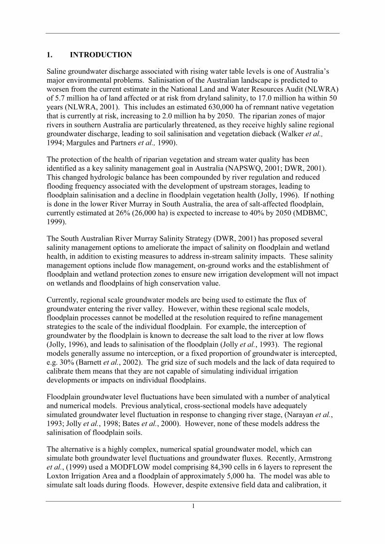
The floodplains have been conceptualised in a simple cross sectional model, comprising a surface layer of Coonambidgal Clay overlying a layer of Monoman Sands (Figure 1). This is based on drilling records (AWE, 1999) and modelling studies around the Bookpurnong and Loxton Irrigation Areas (Barnett et al., 2002; Armstrong et al., 1999). The highland area is represented by the unconfined Upper Loxton (Pliocene) Sands aquifer. Both the highland and floodplain are underlain by the Lower Loxton Sands, a relatively impermeable clayey sand formation.

Figure 1. Conceptual model of groundwater inputs to the floodplain and potential groundwater discharge pathways within the floodplain. Groundwater entering the river valley can be discharged as either seepage at the break of slope, evapotranspiration through the floodplain, or as base flow to the river.

The arrows in Figure 1 represent groundwater flow directions and potential groundwater discharge sites. Groundwater flow in the Upper Loxton Sands is a combination of irrigation recharge and regional groundwater flow. Groundwater from the highlands is discharged as either seepage at the break of slope if the groundwater level is above the surface, evapotranspiration through the floodplain when the water table is within the evapotranspiration extinction depth (vegetation rooting depth), or as base flow to the river.

2.2 Model Assumptions

The following assumptions are made:

1. groundwater flow within the floodplain is one-dimensional, under steady state conditions with no recharge, and the floodplain aquifer is homogenous and isotropic; and

2. groundwater flow under the floodplain is generally defined by Darcy’s Law (1), where Q is the flux of groundwater through a unit width of floodplain [L2 T-1]; K is the horizontal

4

hydraulic conductivity of the aquifer [L T-1]; b is the aquifer thickness [L]; and dh/dx is the groundwater hydraulic gradient, where h is the height of the groundwater above river level [L] and x is the distance from the edge of the river valley [L] to a maximum distance L at the river;

dhQ Kbdx

= − ; (1)

3. Loss of groundwater through evapotranspiration, ET [L T-1] is calculated using the simple linear function described by (2) and (3); where a is the maximum rate of groundwater lost by evapotranspiration at the floodplain surface on an areal basis [L T-1]. This maximum groundwater evapotranspiration rate declines to zero at zext, which corresponds to the vegetation rooting depth; hf is the height of the floodplain above river level [L]; and zext is the evapotranspiration extinction depth [L], or rooting depth, below which there is no evapotranspiration.

( )

f ext

f extext

a h h zET h h z

z

⎡ ⎤− −⎣ ⎦= > − , (2)

0 f extET h h z= ≤ − ; and (3)

4. A sharp cliff and a flat floodplain characterise the shape of the river valley.

2.3 Governing Equations

Under the above assumptions, the generalised flow equation, (1) can be simplified to:

1. groundwater level below the extinction depth, groundwater flow is controlled by hydraulic gradient between the edge of the floodplain and the river, i.e.

( )2

2 0 f extd hKb h h zdx

= ≤ − (4)

2. groundwater level above the extinction depth, groundwater flow is controlled by hydraulic gradient and evapotranspiration across the floodplain, i.e.

( )2

2

( ) ext f

f extext

a z h hd hKb h h zdx z

− += > − . (5)

2.4 Non-Dimensional Equations

The above equations can be written in non-dimensional form in order to:

1. minimise the number of variables, and

2. put into perspective the balance between the different floodplain groundwater discharge processes.

To do this, we substitute the following:

5

* * *, and z 1 ext

f f

h x zh xh L h

= = = −

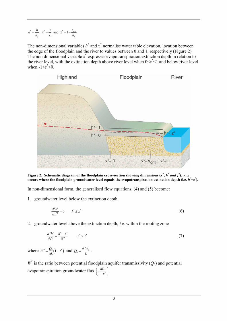
The non-dimensional variables h* and x* normalise water table elevation, location between the edge of the floodplain and the river to values between 0 and 1, respectively (Figure 2). The non dimensional variable z* expresses evapotranspiration extinction depth in relation to the river level, with the extinction depth above river level when 0<z*<1 and below river level when -1<z*<0.

Figure 2. Schematic diagram of the floodplain cross-section showing dimensions (x*, h* and z*). xcrit occurs where the floodplain groundwater level equals the evapotranspiration extinction depth (i.e. h*=z*).

In non-dimensional form, the generalised flow equations, (4) and (5) become:

1. groundwater level below the extinction depth

2 2

* **2 0 d h h z

dx= ≤ (6)

2. groundwater level above the extinction depth, i.e. within the rooting zone

2 * * *

* **2 * d h h z h z

dx W−

= > (7)

where ( )* *0 1QW zaL

= − and 0fKbh

QL

= .

W* is the ratio between potential floodplain aquifer transmissivity (Q0) and potential

evapotranspiration groundwater flux *1aL

z⎛ ⎞⎜ ⎟−⎝ ⎠

.

6

2.5 Boundary Conditions

The river represents a constant head boundary condition, therefore:

0 at h x L= = (8)

or * *0 at 1h x= = (9)

At the edge of the floodplain (i.e. x=0) when there is no seepage, i.e. the water table is below the floodplain surface, the boundary condition is given by:

when in fdhKb Q h hdx

− = ≤ (10)

or *

** when 1in

dh q hdx

= − < , (11)

where Qin is the groundwater flux entering the floodplain and 0

inin

QqQ

= .

The non-dimensional variable qin is the groundwater flux to the floodplain (Qin) normalised with respect to floodplain aquifer transmissivity (Q0).

When the flux of groundwater entering the floodplain is greater than the floodplain can transmit (i.e. qin>1), seepage occurs so that the water table is at the floodplain surface. When seepage occurs, the dimensionless flux at the edge of the floodplain (i.e. x=0) is defined as:

0 when in s fQ Q Q h h= − > (12)

or *0 1 when 1q h= ≥ (13)

where Qs is the flux of groundwater discharged as seepage and q0 is the maximum possible flux through the floodplain aquifer, which is defined as:

* *0 * when 1 at 0dhq h x

dx= − = = (14)

When seepage does not occur, the dimensionless flux at the edge of the floodplain (i.e. x=0) is defined as:

0 = when in fQ Q h h≤ (15)

or *0

0

when 1inQq hQ

= < (16)

We define the possible fluxes through a unit width of floodplain as follows:

1. Seepage at the edge of the floodplain (i.e. x=0)

0 when s in fQ Q Q h h= − ≥ ; (17)

7

or *

0

when 1ss

Qq hQ

= ≥ ; (18)

2. Evapotranspiration across the floodplain

0ET rQ Q Q= − (19)

or 0

ETET

QqQ

= , (20)

where QET is the flux of groundwater lost through evapotranspiration, and Qr is the flux of groundwater discharged to the river as baseflow; and

3. Baseflow to the river (i.e. x=L) is defined as:

when =0rdhQ Kb hdx

= − (21)

or *

**=- when 0r

dhq hdx

= , (22)

where 0

rr

QqQ

= .

The non-dimensional groundwater fluxes express seepage (qs,), evapotranspiration (qET) and baseflow (qr) relative to the maximum flux the floodplain aquifer can transmit (Q0). We are interested in determining the proportion of groundwater discharged as seepage, evapotranspiration and baseflow.

2.6 Floodplain Scenarios

We consider two general situations:

(a) River level below rooting depth (z*>0)

We define a point on the floodplain xcrit (0<xcrit<1) where the floodplain groundwater level equals the evapotranspiration extinction depth (i.e. h*=z*). At any point between xcrit and the river, the groundwater level is below the extinction depth, i.e.

( )* * *1 when 1r crith q x x x= − < < . (23)

Substituting h*=z* and x*=xcrit into (23) allows us to quantify qr for known values of z* and xcrit, i.e.:

( )

*

1rcrit

zqx

=−

. (24)

Integrating (7) gives the following general solutions where B and C are constants:

* *

* *

* *cosh sinhx xh B C z

W W

⎛ ⎞ ⎛ ⎞= + +⎜ ⎟ ⎜ ⎟⎜ ⎟ ⎜ ⎟

⎝ ⎠ ⎝ ⎠ (25)

8

* * *

* * * * *sinh coshdh B x C x

dx W W W W

⎛ ⎞ ⎛ ⎞= +⎜ ⎟ ⎜ ⎟⎜ ⎟ ⎜ ⎟

⎝ ⎠ ⎝ ⎠. (26)

At xcrit when h*=z*, (25) allows B to be expressed in terms of C, xcrit and z*.

Equating (22) and (26) at x*=xcrit gives:

* * * *

sinh coshcrit critr

B x C xqW W W W

⎛ ⎞ ⎛ ⎞− = +⎜ ⎟ ⎜ ⎟⎜ ⎟ ⎜ ⎟

⎝ ⎠ ⎝ ⎠. (27)

Substituting xcrit from (24) and B from (25) gives the following solutions for B and C:

*

*

*sinh r

r

r

q zB q Wq W

⎛ ⎞−⎜ ⎟=⎜ ⎟⎝ ⎠

(28)

and *

*

*cosh r

r

r

q zC q Wq W

⎛ ⎞−⎜ ⎟= −⎜ ⎟⎝ ⎠

. (29)

Equating (16) and (26) for the above solutions of B and C at the edge of the floodplain (x*=0) allows qr to be calculated iteratively from values of q0, z* and W*, i.e.

*

0 *cosh r

r

r

q zq qq W

⎛ ⎞−⎜ ⎟=⎜ ⎟⎝ ⎠

. (30)

If we define the non dimensional height of the water table at the edge of the floodplain as h*=h0 at x*=0, and substitute into (25), then:

*

* *0 *

sinh rr

r

q zh q W zq W

⎛ ⎞−⎜ ⎟= +⎜ ⎟⎝ ⎠

. (31)

Therefore, when h0=1, i.e. the water table is at the floodplain surface, the flux to the river can be calculated from z* and W*:

*

* *

*1 sinh r

r

r

q zz q Wq W

⎛ ⎞−⎜ ⎟− =⎜ ⎟⎝ ⎠

. (32)

When seepage does not occur, the value of xcrit can be determined by matching values of q0 and qin when (24) is substituted into (30). This value of xcrit can then be used to calculate qr from (24). When seepage occurs, qr can be determined from (32). Using this value of qr, q0 can then be calculated from (30).

(b) River level within rooting depth (z*<h*)

Equating (22) and (26) at the river (x*=1) gives:

* * * *

1 1sinh coshrB CqW W W W

⎛ ⎞ ⎛ ⎞= − −⎜ ⎟ ⎜ ⎟⎜ ⎟ ⎜ ⎟

⎝ ⎠ ⎝ ⎠ (33)

9

Equating (16) and (26) at the edge of the floodplain (x*=0), we can derive an equation to describe C:

0 *

CqW

= − (34)

i.e. *0C q W= −

Substituting C into (25) at the river, when x*=1 and h*=0 gives:

* *0* *

1 10 cosh sinhB q W zW W

⎛ ⎞ ⎛ ⎞= − +⎜ ⎟ ⎜ ⎟⎜ ⎟ ⎜ ⎟

⎝ ⎠ ⎝ ⎠ (35)

i.e. * *

0 *

*

1sinh

1cosh

q W zWB

W

⎛ ⎞−⎜ ⎟⎜ ⎟

⎝ ⎠=⎛ ⎞⎜ ⎟⎜ ⎟⎝ ⎠

.

We can then solve for qr by substituting B and C into (33).

* *

0 *

**

1sinh

1coshr

q W zWq

WW

⎛ ⎞+ ⎜ ⎟⎜ ⎟

⎝ ⎠=⎛ ⎞⎜ ⎟⎜ ⎟⎝ ⎠

(36)

When qr is negative, the location of the groundwater divide, xdiv (0<xdiv<1) can be calculated from (26) for known values of z*, q0 and W*.

* *

* *0

*

1cosh1sinh

tanh div

z Wxq W WW

⎛ ⎞⎜ ⎟⎜ ⎟⎛ ⎞ ⎝ ⎠= −⎜ ⎟⎜ ⎟ ⎛ ⎞⎝ ⎠ ⎜ ⎟⎜ ⎟⎝ ⎠

(37)

By substituting B into (25), the height of the water table at the edge of the floodplain (x*=0) can be calculated from values of q0, W* and z*.

* *

0 **

0

*

1sinh

1cosh

q W zWh z

W

⎛ ⎞−⎜ ⎟⎜ ⎟

⎝ ⎠= +⎛ ⎞⎜ ⎟⎜ ⎟⎝ ⎠

. (38)

Therefore, when h0=1, i.e. the water table is at the floodplain surface, q0 can be calculated from z* and W*:

* *

0 **

*

1sinh1

1cosh

q W zWz

W

⎛ ⎞−⎜ ⎟⎜ ⎟

⎝ ⎠− =⎛ ⎞⎜ ⎟⎜ ⎟⎝ ⎠

. (39)

10

When seepage does not occur, qr can be calculated from (36) using q0=qin. When seepage occurs, q0 can be determined from (39). Using this value of q0, qr can be calculated from (36).

2.7 Model Comparison

The analytical model was compared to the numerical groundwater flow model, MODFLOW over a range of possible scenarios. Both models simulated a simple cross-sectional area of highland and floodplain (Figure 1). Modelling scenarios representing up and downstream of a weir; uncleared, cleared and irrigated highland recharge; 5 floodplain widths (L); and two maximum floodplain evapotranspiration rates (a) were used. For each of the 30 scenarios, the MODFLOW cell-by-cell estimates of flux entering the river valley (Qin), flux of groundwater lost as seepage from the seepage cell at the edge of the highland (Qs), evapotranspiration (QET) and as base flow to the river (Qr) were recorded and compared to the analytical model estimates.

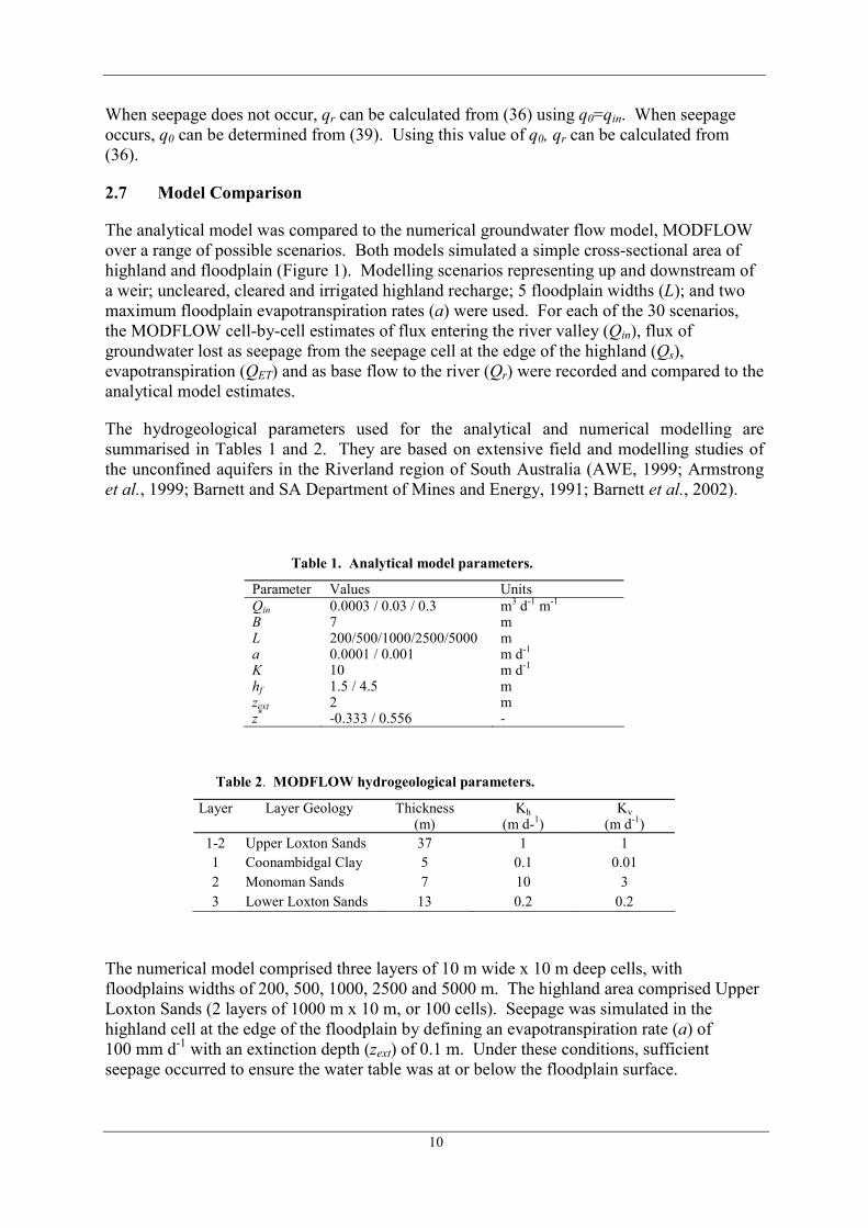
The hydrogeological parameters used for the analytical and numerical modelling are summarised in Tables 1 and 2. They are based on extensive field and modelling studies of the unconfined aquifers in the Riverland region of South Australia (AWE, 1999; Armstrong et al., 1999; Barnett and SA Department of Mines and Energy, 1991; Barnett et al., 2002).

Table 1. Analytical model parameters.

Parameter Values Units Qin 0.0003 / 0.03 / 0.3 m3 d-1 m-1 B 7 m L 200/500/1000/2500/5000 m a 0.0001 / 0.001 m d-1 K 10 m d-1 hf 1.5 / 4.5 m zext 2 m z* -0.333 / 0.556 -

Table 2. MODFLOW hydrogeological parameters.

Layer Layer Geology Thickness (m)

Kh (m d-1)

Kv (m d-1)

1-2 Upper Loxton Sands 37 1 1 1 Coonambidgal Clay 5 0.1 0.01 2 Monoman Sands 7 10 3 3 Lower Loxton Sands 13 0.2 0.2

The numerical model comprised three layers of 10 m wide x 10 m deep cells, with floodplains widths of 200, 500, 1000, 2500 and 5000 m. The highland area comprised Upper Loxton Sands (2 layers of 1000 m x 10 m, or 100 cells). Seepage was simulated in the highland cell at the edge of the floodplain by defining an evapotranspiration rate (a) of 100 mm d-1 with an extinction depth (zext) of 0.1 m. Under these conditions, sufficient seepage occurred to ensure the water table was at or below the floodplain surface.

11

In the floodplain portion of the model, Layer 1 consisted of Coonambidgal Clay (from 200 m to 5000 m in width, or 20 to 500 cells), overlying Monoman Sands. Lower Loxton Sands comprised Layer 3 of the highland and floodplain regions of the model. Recharge rates representing uncleared (1.1 mm yr–1 (Allison et al., 1990)), cleared (11 mm yr–1 (Allison et al., 1990)) and irrigated (110 mm yr–1 (Armstrong et al., 1999)) land use were used in the 1000 m wide highland portion of the model.

Evapotranspiration in the floodplain cells was defined as 0.1 mm d-1 and 1.0 mm d–1, with an extinction depth of 2 m. Peck (1978) suggested that 0.1 mm d-1 was an empirically derived critical dryland evapotranspiration rate, for the assessment of salinity hazard on non-irrigated land in a Mediterranean climate. This corresponds to the rate of groundwater loss by evapotranspiration from floodplain black box (Eucalyptus largiflorens) woodlands overlying saline groundwater (24 – 33 dS m-1) measured by Thorburn et al. (1993). Similarly, Talsma (1963) reported that 1.0 mm d–1 was an empirically derived, critical rate for irrigated soils overlying a shallow saline aquifer. This corresponds to the values measured by Thorburn et al. (1993) for floodplain red gums (E. camaldulensis) overlying moderately saline groundwater (11 dS m-1). Floodplain evapotranspiration rates are therefore likely to lie between 0.1 mm d-1 and 1.0 mm d-1.

Starting heads were defined over the entire model as equal to the elevation of the constant head in the river cell. The river was simulated in the last cell of Layer 2, using a constant head of 4.5 m (downstream) or 1.5 m (upstream) below the floodplain surface. This is 2.5 m below and 0.5 m above the evapotranspiration extinction depth for the downstream and upstream scenarios, respectively. The cell in Layer 1 above the river cell was designated as no flow. Note that the numerical model was not calibrated in the traditional sense, as the purpose of the numerical modelling was to calculate groundwater fluxes for a range of scenarios for comparison with analytical model predictions.

2.8 Results

Analytical model estimates of floodplain groundwater discharge patterns were compared to those predicted by MODFLOW for each of the 30 scenarios. The analytical model estimates of seepage, evapotranspiration and base flow fluxes per unit width of aquifer (ML yr-1) were consistent with those of MODFLOW over a broad range of floodplain physical and hydraulic parameters. The regression was statistically significant (n=90, R2=0.998, P<0.001**).

0.99 0.23MODFLOW Analytical= + (40)

Seepage was predicted in 6 scenarios, characterised by large groundwater inputs from irrigation, wide floodplains and low evapotranspiration rates.

The numerical model was sensitive to starting heads, despite steady state conditions. Generally, initial conditions are not important for steady-state simulations, however they can be important in certain non-linear situations where flux, transmissivity, or saturation are a function of head (McDonald and Harbaugh, 1988). A sensitivity analysis was not performed for the numerical model. However, the analytical model provides the means for analysis of the sensitivity of modelling parameters to final groundwater discharge estimates.

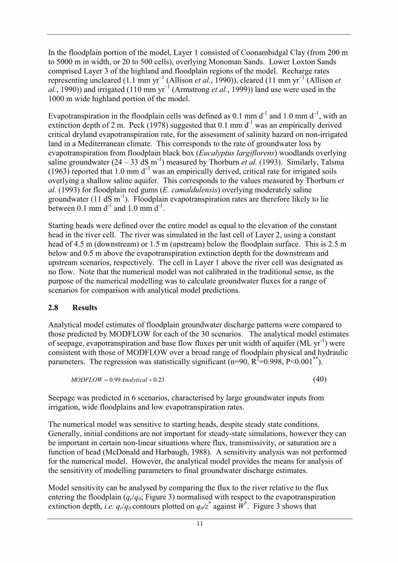
Model sensitivity can be analysed by comparing the flux to the river relative to the flux entering the floodplain (qr/q0; Figure 3) normalised with respect to the evapotranspiration extinction depth, i.e. qr/q0 contours plotted on q0/z* against W*. Figure 3 shows that

12

groundwater modelling is sensitive when the contours of the predicted ratio of qr/q0 are close. This occurs for small, negative values of q0/z* and large W* values, which occurs when the floodplain aquifer transmissivity is less than the potential evapotranspiration rate, e.g. wide floodplains, high fluxes into the floodplain and river levels above the evapotranspiration extinction depth. Large positive and negative values of q0/z* and small W* values also cause models to be sensitive to parameter selection. These conditions occur when there are high potential evapotranspiration fluxes, and the flux entering the floodplain is greater than floodplain aquifer transmissivity.

Figure 3. Model parameter sensitivity diagram showing qr/q0 contours (—) plotted on q0/z* and W* axes to normalise the values with respect to the evapotranspiration extinction depth. The qr/q0 contours (—) show when groundwater models (q0/z* and W*) are sensitive to parameter estimation.

13

3. PART II: APPLICATION TO THE LOWER RIVER MURRAY, AUSTRALIA

3.1 Site Description

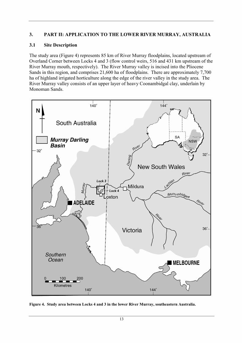
The study area (Figure 4) represents 85 km of River Murray floodplains, located upstream of Overland Corner between Locks 4 and 3 (flow control weirs, 516 and 431 km upstream of the River Murray mouth, respectively). The River Murray valley is incised into the Pliocene Sands in this region, and comprises 21,600 ha of floodplains. There are approximately 7,700 ha of highland irrigated horticulture along the edge of the river valley in the study area. The River Murray valley consists of an upper layer of heavy Coonambidgal clay, underlain by Monoman Sands.

Figure 4. Study area between Locks 4 and 3 in the lower River Murray, southeastern Australia.

14

3.2 Methodology

The floodplain was divided into 447 divisions of approximately 250 m width based on floodplain groundwater flow paths between the edge of the river valley and the river. Within the study area, the following allowed the model to be tested and validated against ‘real’ data:

1. A range of possible river regulation impacts from immediately upstream of Lock 3 to downstream of Lock 4;

2. Irrigated and non-irrigated highland areas;

3. Floodplain widths up to 5,700 m; and

4. Measured river salt loads at kilometre intervals and detailed floodplain tree health maps.

3.3 Groundwater Inflows

Groundwater inflows were calculated from highland groundwater gradients, and regional aquifer hydraulic conductivity and thickness. Regional hydraulic conductivity ranges between 1 and 5 m d-1 (Barnett and SA Department of Mines and Energy, 1991). Highland groundwater gradients were estimated from groundwater contours, which were interpolated from measured groundwater depths in regional bores. The total flux to each floodplain division was calculated from the flux per unit width (Qin) and the width of the floodplain at the edge of the river valley (Ledge).

All regional and floodplain aquifer parameters are described in Table 3 and were derived from reported field and modelling studies (Barnett and SA Department of Mines and Energy, 1991; Armstrong et al., 1999; Barnett et al., 2002).

Table 3. Description and method of estimation of model parameters.

Parameter Description and Method of Estimation Qin Groundwater flux per unit width of floodplain (Qin = Kh*Ih*th, m2 d-1) Kh Highland aquifer hydraulic conductivity (constant, Kh = 2 m d-1) Ih Highland groundwater gradient from interpolated groundwater contours th Highland aquifer thickness at edge of the river valley (constant, th = 10 m)

Ledge Floodplain width at edge of the river valley (m) Kf Floodplain aquifer hydraulic conductivity (constant, Kf = 10 m d-1) b Floodplain aquifer thickness from drilling records (constant, b = 5 m) hf Difference between elevation of a 100 GL d-1 flood and river level at entitlement flow (m) L Average length of division sides between the edge of the river valley and the river (m) a Maximum floodplain evapotranspiration rate (constant, a = 0.0001 m d-1)

zext Floodplain evapotranspiration extinction depth (constant, zext = 2 m) Cgw Floodplain groundwater salinity (ranges from 10,650 to 42,450 mg L-1)

The distance between the edge of the river valley and the river (L) was calculated from an average of the two division sides. The difference between the elevation of a 100 GL d-1 flood at the edge of the floodplain (modelled floodplain surface) and the river elevation at entitlement flow (hf) was also calculated from GIS elevation data (Overton et al., 1999) for each division.

15

Evapotranspiration parameters were set to constant values based on measured lower River Murray floodplain soil- and vegetation- limited groundwater discharge rates (Jolly et al., 1993; Thorburn et al., 1993). Floodplain groundwater salinities (Cgw) were interpolated from measured values.

Ideally, model estimates of groundwater discharge fluxes would be compared to measured, field validated groundwater discharge fluxes. However, field measurements of seepage, groundwater losses by evapotranspiration and base flow groundwater discharge fluxes are not available or easily measured at a regional scale. Instead, surrogate measures of groundwater discharge fluxes: observed seepage areas, tree health and river salt loads, were used to evaluate model predictions.

Groundwater inflows from interpolated contours were calibrated against known conditions to assist in determining correct groundwater inflows. In many areas, groundwater depths were missing, so groundwater inflows were estimated from irrigation history and by matching the observed patterns and magnitude of salt loads. These current groundwater inflows represent the best estimate for the study area.

3.4 Floodplain Vegetation Health

Floodplain vegetation health was mapped in ~40% of the study area (PPK, 1997; 1998; AWE, 2000). This GIS coverage includes ~3,500 ha of trees and ~5,000 ha of other vegetation, including shrubs, ground covers and wetland species.

The vegetation mapping was completed over all of the floodplain to the south of the river and several floodplains on the northern side of the river. Predominant tree communities in the study area include black box (Eucalyptus largiforens), red gum (E. camaldulensis) and cooba (Acacia stenophylla). Due to the complexity of floodplain vegetation associations, only tree health (rated as healthy, poor health, or dead) was used in this analysis.

Areas where seepage was observed, including seepage faces and areas of reeds were mapped from ground surveys and aerial photography. Observed seepage areas were compared to predicted seepage areas for a range of groundwater inflow scenarios. Seepage assessments of tree health were limited to within 100 m of the edge of the river valley. Areas where the floodplain was <100 m wide were considered separately due to possible bank recharge influences on vegetation health.

The parameter xcrit was used to assess when vegetation was at risk of salinisation associated with groundwater discharge. For divisions where xcrit>0, the floodplain cannot transmit incoming groundwater and evapotranspiration occurs, causing the floodplain water table to rise to within 2 m (zext) of the surface. Evapotranspiration predictions were compared to tree health in the middle of the floodplain, excluding a buffer within 100 m of the river and 100 m from the edge of the river valley. These buffer zones represent areas where floodplain tree health is influenced by proximity to the river or edge of the river valley, rather than salinisation associated with groundwater discharge by evapotranspiration.

3.5 River Salt Loads

Model estimates of base flow were converted from the flux of groundwater discharged to the river per division (m3 d-1) to tons of salt using interpolated floodplain groundwater salinities

16

(mg L-1). These salt loads were assigned to the nearest river km for each division as tons of salt entering the river per km per day for each river kilometre.

Salt loads were compared to measured ‘Run of River’ salt loads determined from river flow rates and in stream salinity measurements taken over 5 years at low flows (DWR, 2001b; Porter, 2001). An average of 5 ‘Run of River’ salt loads was used to estimate long-term salt accessions. The variability of salt loads measured depended on recent (6-18 months) flow history, particularly in areas with large permanently inundated wetlands upstream of Lock 3.

17

4. RESULTS

Model results for different groundwater inflow scenarios were compared to observed seepage areas, mapped tree health and measured river salt loads between Locks 4 and 3 in the lower River Murray.

4.1 Seepage

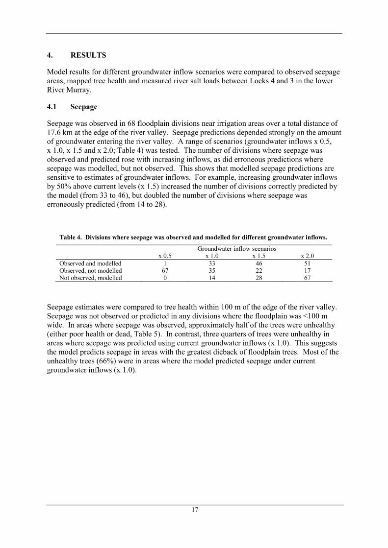
Seepage was observed in 68 floodplain divisions near irrigation areas over a total distance of 17.6 km at the edge of the river valley. Seepage predictions depended strongly on the amount of groundwater entering the river valley. A range of scenarios (groundwater inflows x 0.5, x 1.0, x 1.5 and x 2.0; Table 4) was tested. The number of divisions where seepage was observed and predicted rose with increasing inflows, as did erroneous predictions where seepage was modelled, but not observed. This shows that modelled seepage predictions are sensitive to estimates of groundwater inflows. For example, increasing groundwater inflows by 50% above current levels (x 1.5) increased the number of divisions correctly predicted by the model (from 33 to 46), but doubled the number of divisions where seepage was erroneously predicted (from 14 to 28).

Table 4. Divisions where seepage was observed and modelled for different groundwater inflows.

Groundwater inflow scenarios x 0.5 x 1.0 x 1.5 x 2.0 Observed and modelled 1 33 46 51 Observed, not modelled 67 35 22 17 Not observed, modelled 0 14 28 67

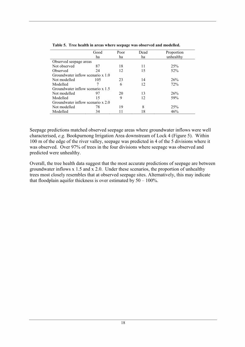
Seepage estimates were compared to tree health within 100 m of the edge of the river valley. Seepage was not observed or predicted in any divisions where the floodplain was <100 m wide. In areas where seepage was observed, approximately half of the trees were unhealthy (either poor health or dead, Table 5). In contrast, three quarters of trees were unhealthy in areas where seepage was predicted using current groundwater inflows (x 1.0). This suggests the model predicts seepage in areas with the greatest dieback of floodplain trees. Most of the unhealthy trees (66%) were in areas where the model predicted seepage under current groundwater inflows (x 1.0).

18

Table 5. Tree health in areas where seepage was observed and modelled.

Good Poor Dead Proportion ha ha ha unhealthy Observed seepage areas Not observed 87 18 11 25% Observed 24 12 15 52% Groundwater inflow scenario x 1.0 Not modelled 105 23 14 26% Modelled 7 6 12 72% Groundwater inflow scenario x 1.5 Not modelled 97 20 13 26% Modelled 15 9 12 59% Groundwater inflow scenario x 2.0 Not modelled 78 19 8 25% Modelled 34 11 18 46%

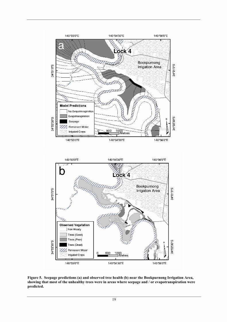
Seepage predictions matched observed seepage areas where groundwater inflows were well characterised, e.g. Bookpurnong Irrigation Area downstream of Lock 4 (Figure 5). Within 100 m of the edge of the river valley, seepage was predicted in 4 of the 5 divisions where it was observed. Over 97% of trees in the four divisions where seepage was observed and predicted were unhealthy.

Overall, the tree health data suggest that the most accurate predictions of seepage are between groundwater inflows x 1.5 and x 2.0. Under these scenarios, the proportion of unhealthy trees most closely resembles that at observed seepage sites. Alternatively, this may indicate that floodplain aquifer thickness is over estimated by 50 – 100%.

19

Figure 5. Seepage predictions (a) and observed tree health (b) near the Bookpurnong Irrigation Area, showing that most of the unhealthy trees were in areas where seepage and / or evapotranspiration were predicted.

20

4.2 Evapotranspiration

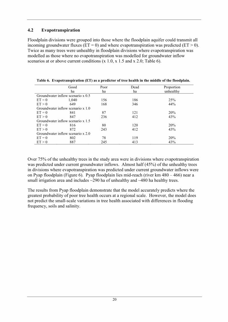
Floodplain divisions were grouped into those where the floodplain aquifer could transmit all incoming groundwater fluxes (ET = 0) and where evapotranspiration was predicted (ET > 0). Twice as many trees were unhealthy in floodplain divisions where evapotranspiration was modelled as those where no evapotranspiration was modelled for groundwater inflow scenarios at or above current conditions (x 1.0, x 1.5 and x 2.0; Table 6).

Table 6. Evapotranspiration (ET) as a predictor of tree health in the middle of the floodplain.

Good Poor Dead Proportion ha ha ha unhealthy Groundwater inflow scenario x 0.5 ET = 0 1,040 156 186 25% ET > 0 649 168 346 44% Groundwater inflow scenario x 1.0 ET = 0 841 87 121 20% ET > 0 847 236 412 43% Groundwater inflow scenario x 1.5 ET = 0 816 80 120 20% ET > 0 872 243 412 43% Groundwater inflow scenario x 2.0 ET = 0 802 78 119 20% ET > 0 887 245 413 43%

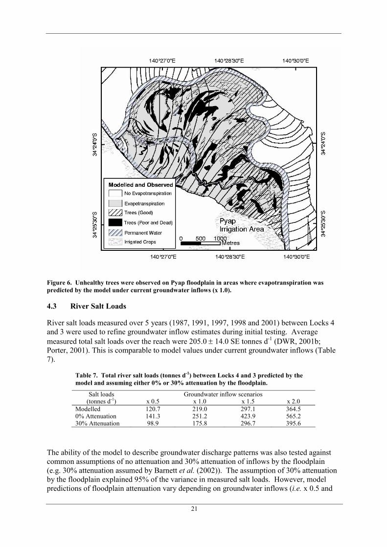
Over 75% of the unhealthy trees in the study area were in divisions where evapotranspiration was predicted under current groundwater inflows. Almost half (45%) of the unhealthy trees in divisions where evapotranspiration was predicted under current groundwater inflows were on Pyap floodplain (Figure 6). Pyap floodplain lies mid-reach (river km 480 – 466) near a small irrigation area and includes ~290 ha of unhealthy and ~480 ha healthy trees.

The results from Pyap floodplain demonstrate that the model accurately predicts where the greatest probability of poor tree health occurs at a regional scale. However, the model does not predict the small-scale variations in tree health associated with differences in flooding frequency, soils and salinity.

21

Figure 6. Unhealthy trees were observed on Pyap floodplain in areas where evapotranspiration was predicted by the model under current groundwater inflows (x 1.0).

4.3 River Salt Loads

River salt loads measured over 5 years (1987, 1991, 1997, 1998 and 2001) between Locks 4 and 3 were used to refine groundwater inflow estimates during initial testing. Average measured total salt loads over the reach were 205.0 ± 14.0 SE tonnes d-1 (DWR, 2001b; Porter, 2001). This is comparable to model values under current groundwater inflows (Table 7).

Table 7. Total river salt loads (tonnes d-1) between Locks 4 and 3 predicted by the model and assuming either 0% or 30% attenuation by the floodplain.

Salt loads Groundwater inflow scenarios (tonnes d-1) x 0.5 x 1.0 x 1.5 x 2.0

Modelled 120.7 219.0 297.1 364.5 0% Attenuation 141.3 251.2 423.9 565.2 30% Attenuation 98.9 175.8 296.7 395.6

The ability of the model to describe groundwater discharge patterns was also tested against common assumptions of no attenuation and 30% attenuation of inflows by the floodplain (e.g. 30% attenuation assumed by Barnett et al. (2002)). The assumption of 30% attenuation by the floodplain explained 95% of the variance in measured salt loads. However, model predictions of floodplain attenuation vary depending on groundwater inflows (i.e. x 0.5 and

22

x 1.0 <30%, x 1.5 ~30%, and x 2.0 >30%; Table 7). In addition, this simple approximation does not indicate where salinisation associated with seepage or high rates of evapotranspiration occurs, or how these patterns change with the magnitude of groundwater inflows.

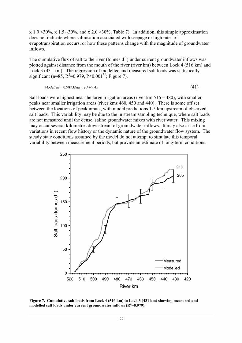
The cumulative flux of salt to the river (tonnes d-1) under current groundwater inflows was plotted against distance from the mouth of the river (river km) between Lock 4 (516 km) and Lock 3 (431 km). The regression of modelled and measured salt loads was statistically significant (n=85, R2=0.979, P<0.001**; Figure 7).

0.987 9.45Modelled Measured= + (41)

Salt loads were highest near the large irrigation areas (river km 516 – 480), with smaller peaks near smaller irrigation areas (river kms 460, 450 and 440). There is some off set between the locations of peak inputs, with model predictions 1-5 km upstream of observed salt loads. This variability may be due to the in stream sampling technique, where salt loads are not measured until the dense, saline groundwater mixes with river water. This mixing may occur several kilometres downstream of groundwater inflows. It may also arise from variations in recent flow history or the dynamic nature of the groundwater flow system. The steady state conditions assumed by the model do not attempt to simulate this temporal variability between measurement periods, but provide an estimate of long-term conditions.

Figure 7. Cumulative salt loads from Lock 4 (516 km) to Lock 3 (431 km) showing measured and modelled salt loads under current groundwater inflows (R2=0.979).

23

4.4 Sensitivity Analysis

Surrogate measures of groundwater discharge were used to assess model sensitivity to parameterization. This showed that calculation of groundwater fluxes entering the river valley (Qin), particularly near irrigation areas was critical. Those floodplains where groundwater contours were well documented (particularly near large irrigation areas) were accurately predicted. In contrast, estimates of Qin near smaller irrigation areas where regional bores were absent relied on estimates from irrigation area history and observations of floodplain vegetation and salt loads.

Seepage predictions suggested that floodplain aquifer thickness was under estimated by 50 – 100%. The presence of backwaters near many of the observed seepage areas and bore logs (AWE, 1999) in some of these areas suggest that seepage often occurs when groundwater flow is impeded by a thickening of the clay layer near the edge of the river valley. The model does not simulate possible thinning of the floodplain aquifer associated with geomorphologic features.

Evapotranspiration predictions were relatively insensitive to groundwater inflows, being similar for groundwater inflow scenarios at or above current conditions (x 1.0, x 1.5 and x 2.0). In these three scenarios, divisions where evapotranspiration was predicted contained twice as many unhealthy trees.

Salt loads were sensitive to estimates of groundwater inflows. The model estimates of current salt loads exceeded measured salt loads in downstream portions of the study area (river km 460 – 431). This part of the study area is characterised by permanently inundated wetlands and greater variability of the kilometre-by-kilometre river salinity data (Figure 7). It is likely that these wetlands act as salt stores, intercepting groundwater discharge and thereby minimizing salt loads in the river channel during low flows.

24

5. DISCUSSION

The scenarios used to compare the analytical and MODFLOW models are representative of the conditions experienced in the lower River Murray. They are based on previously reported regional values for the area and represent a broad range of likely modelling scenarios. Therefore, the analytical model can also be applied to other scenarios where the basic conceptual model of a gaining stream holds, but recharge rates and aquifer properties differ.

The analytical model also gives an indication of the sensitivity of groundwater modelling to the selection of modelling parameters. It indicates that modelling parameters should be chosen carefully for scenarios where fluxes to the floodplain are greater than aquifer transmissivity normalised with respect to evapotranspiration extinction depth (large q0/z*) and where potential evapotranspiration rates greatly exceed floodplain aquifer transmissivity (small W*). Modelling parameters with these conditions result in significant proportions of groundwater being discharged as seepage and evapotranspiration, affecting baseflow estimates.

In Part II, when the analytical model was applied to the lower River Murray, the accuracy of seepage predictions was strongly dependent on the estimates of current groundwater inflows. Higher groundwater fluxes to the river valley resulted in greater success in predicting seepage areas, but increased errors, i.e. seepage modelled, but not observed. Model predictions of seepage areas encompassed most of the unhealthy trees (66%) under current groundwater inflows (x 1.0). It is suggested that thinning of the floodplain aquifer might contribute to observed but not predicted seepage in areas near backwaters under current groundwater inflows. Thick clay lenses were observed in bore logs from seepage areas near backwaters in the study area.

Over 75% of the unhealthy trees in the study area were in divisions where evapotranspiration was predicted. The model predicts evapotranspiration when floodplain water levels are within the extinction depth (zext). This occurs when groundwater inflows approach the floodplain aquifer transmissivity or the river level is near the extinction depth. In both situations, soil limited groundwater discharge becomes a significant component of the water balance. This suggests that salinisation associated with groundwater discharge by evapotranspiration is the principle process driving floodplain vegetation health, despite the complex interactions between floodplain geomorphology, flooding and land use history on vegetation health. This indicates the usefulness of this modelling approach for predicting floodplain vegetation responses to management.

The overall pattern and magnitude of modelled salt load predictions are comparable to the measured values, which is more accurate than simply assuming that 30% of groundwater inflows are attenuated by the floodplain. This means that the model can be used to predict future salt loads from new irrigation developments and can also be used as a planning tool to identify the impact of proposed developments on floodplain and wetland health and river salinity.

In areas upstream from locks, where the river level is within the evapotranspiration extinction depth, high evapotranspiration rates across the floodplain are predicted. Not surprisingly, in these scenarios the model is sensitive to small errors in parameterisation and conceptualisation. Small changes to model parameters (hf, zext, L, and a) can change model predictions from small fluxes to the river, to large fluxes from the river into the floodplain.

25

Therefore, model predictions need to be tested against independently measured field data (observed seepage, tree health and river salt loads) to ensure that accurate predictions are made.

The model presented in this report does not attempt to simulate floodplain wetlands, backwaters or oxbows, which occur as the river meanders across the floodplain. This is because the role that these water bodies play in intercepting saline groundwater flowing towards the river is still unknown. The analysis of seepage predictions under current groundwater inflows also highlighted the need to determine the role that aquifer thinning near backwaters plays in groundwater being discharged as seepage. This is an area of future research, and has the potential to refine the model’s estimates of seepage, salt loads and evapotranspiration flux through the floodplains.

26

6. CONCLUSIONS

A simple, one dimensional, cross-sectional analytical model of a low land river floodplain was comparable to MODFLOW numerical estimates of patterns of groundwater discharge. The models predicted groundwater discharge as seepage at the break of slope, evapotranspiration through the floodplain and base flow to the river. However, the analytical model computing requirements were lower and the required data inputs could be obtained from published regional scale information.

The model was applied to a study area comprising 85 km of floodplains in the lower River Murray, south eastern Australia. The model’s predictions provided good correlations with observed seepage areas, vegetation health data and measured salt loads to the river. Model predictions of seepage areas were sensitive to estimates of groundwater inflows. Observations of floodplain geomorphology and poor prediction of some seepage areas suggested that seepage might be associated with floodplain aquifer thinning near backwaters. This requires further investigation and conceptualisation.

Over 75% of the unhealthy trees in the study area were in divisions where evapotranspiration was predicted. This suggests that salinisation associated with groundwater discharge by evapotranspiration is the principle process driving floodplain vegetation health, despite the complex interactions between floodplain geomorphology, flooding and land use history on vegetation health.

The model has shown that with good groundwater inflow data, it is capable of predicting kilometre-by-kilometre salt loads to identify ‘hotspots’ of salt input to the river. Model predictions of salt loads are more accurate under a range of groundwater inflow scenarios than simply assuming that 30% of groundwater inflows are attenuated by the floodplain.

The model highlights the physical relationships that exist between floodplain variables in the calculation of interception of groundwater by the floodplain. The model is sensitive to parameterisation when the river level or floodplain water level is within the evapotranspiration extinction depth. This is typical of conditions upstream of weirs and near irrigation areas.

The approach described in this report can be applied more broadly, although the impact of wetlands and oxbows, which may act to intercept groundwater within the floodplain, is not taken into account. The model provides a tool to address the management of floodplain and wetland health and river salinity. It can also be used to identify environmental protection zones for a range of groundwater inflow scenarios.

27

7. REFERENCES

Allison, GB, Cook, PG, Barnett, SR, Walker, GR, Jolly, ID & Hughes, MW 1990, Land clearance and river salinisation in the Western Murray basin, Australia, J. Hydrol., 119, 1-20.

Armstrong, D, Yan, W & Barnett, SR 1999, Loxton Irrigation Area - Groundwater Modelling of Groundwater / River Interaction. Department of Primary Industries and Resources, Adelaide.

AWE 1999, Clarks Floodplain Investigations. Prepared for the Loxton to Bookpurnong Local Action Planning Committee. Australian Water Environments Report No. 98.031-2, Adelaide.

AWE 2000, Pyap to Overland Corner Floodplain Assessment Report, Prepared for the Loxton to Bookpurnong Local Action Planning Committee, Australian Water Environments Report No. 98027, Adelaide.

Barnett, SR & SA Department of Mines and Energy 1991, Renmark Hydrogeological Map (1:250,000 Scale), Bureau of Mineral Resources, Geol. and Geophysics, Canberra.

Barnett, SR 1989, The effect of land clearance in the Mallee region on River Murray salinity and land salinisation, BMR J. Aust. Geol. and Geophysics, 11, 205-208.

Barnett, SR, Yan, W, Watkins, NR, Woods, JA & Hyde, KM 2002, Murray Darling Basin salinity audit: Groundwater modelling to predict future salt loads to the River Murray in South Australia. Department of Primary Industries and Resources Report DWR 2001/017, Adelaide.

Bates, PD, Stewart, MD, Desitter, A, Anderson, MG, Renaud, J-P & Smith, JA 2000, Numerical simulation of floodplain hydrology. Water Resour. Res., 36, 2517-2529.

Bone B & Davies, G 1992, Effects of irrigation on riparian vegetation in the South Australian Riverland, SA Dept. Ag, Loxton.

DWR 2001a, South Australian River Murray Salinity Strategy 2001 – 2015, Dept. Water Resour., Govt. South Aust., Adelaide.

DWR 2001b, Unpublished Data, Dept. Water Resour., Govt. South Aust., Adelaide.

Jolly, ID, Walker, GR & Thorburn, PG 1993, Salt accumulation in semi-arid floodplain soils with implications for forest health, J. Hydrol., 150, 589-614.

Jolly, ID, Narayan, KA, Armstrong, D & Walker, GR 1998, The impact of flooding on modelling salt transport processes to streams, Env. Model. and Software, 13, 87-104.

Jolly, ID 1998, The Effects of River Management on the Hydrology and Hydroecology of Arid and Semi-Arid Floodplains, in Floodplain Processes, edited by M. G. Anderson, D. E. Walling and P. D. Bates, pp. 577-609, John Wiley & Sons Ltd, New York.

Margules and Partners, P. and J. Smith Ecological Consultants & Victorian Department of Conservation, Forests and Lands 1990, Riparian Vegetation of the River Murray. Murray Darling Basin Commission, Canberra.

McDonald, MC & Harbaugh, AW 1988, A modular three-dimensional finite-difference ground-water flow model, USGS Tech. Water Resour. Invest., Chapter. A1, Book 6.

28

MDBMC 1999, The Salinity Audit of the Murray-Darling Basin. A 100-year perspective, Murray-Darling Basin Ministerial Council, Canberra.

NAPSWQ 2001, Our vital resources: A national action plan for salinity and water quality in Australia, Comm. Aust., Canberra.

Narayan, KA, Jolly, ID & Walker, GR 1993, Predicting flood-driven water table fluctuations in a semi-arid floodplain of the River Murray using a simple analytical model, CSIRO Div. Water Resour. Report 93/2, Adelaide.

NLWRA 2001, Australian dryland salinity assessment 2000. Extent, impacts, processes, monitoring and management options, National Land and Water Resources Audit, Canberra.

Overton, IC, Newman, B, Erdmann, B, Sykora, N & Slegers, S 1999, Modelling floodplain inundation under natural and regulated flows in the Lower River Murray, paper presented at the 2nd Australian Stream Management Conference, Adelaide, February, 1999.

Peck, AJ 1978, Note on the role of a shallow aquifer in dryland salinity, Aust. J. Soil Res., 16, 237-240.

Porter, B 2001, Run of River Salinity Surveys. A method of measuring salt load accessions to the River Murray on a kilometre by kilometre basis, paper presented at Murray Darling Basin Groundwater Workshop; Victor Harbour, South Australia, September, 2001.

PPK 1997, Assessment of the impact of the Loxton Irrigation District on floodplain health and implications for future options, PPK Environment and Infrastructure Report No. 27J121A 97-542, Adelaide.

PPK 1998, Assessment of the impact of the Bookpurnong / Lock 4 Irrigation District on floodplain health and implications for future options. PPK Environment and Infrastructure Report No. 27K055A 98-422, Adelaide.

Talsma, T 1963, The control of saline groundwater. Meded. Landbouwhogesch. Wageningen, 63, 1-68.

Thorburn, PJ, Hatton, TJ & Walker, GR 1993, Combining measurements of transpiration and stable isotopes of water to determine groundwater discharge from forests, J. Hydrol., 150, 563-587.

Walker, GR, Jolly, ID & Jarwal, SD 1994, Salt and water movement in a saline semi arid floodplain of the River Murray, editors, CSIRO Div. Water Resour Report 15, Adelaide.