An Analytic Solution to the Coupled Pressure-Temperature ...utdallas.edu/~sminkoff/save_papers/JEngMathRevised.pdf · An Analytic Solution to the Coupled Pressure-Temperature Equations

Noname manuscript No.(will be inserted by the editor)

An Analytic Solution to the Coupled Pressure-Temperature Equationsfor Modeling of Photoacoustic Trace Gas Sensors

Jordan Kaderli · John Zweck · Artur Safin · Susan E.Minkoff

the date of receipt and acceptance should be inserted later

Abstract Trace gas sensors have a wide range of applications including air quality monitoring, industrialprocess control, and medical diagnosis via breath biomarkers. Quartz-enhanced photoacoustic spectroscopyand resonant optothermoacoustic detection are two techniques with several promising advantages. Bothmethods use a quartz tuning fork and modulated laser source to detect trace gases. To date, these comple-mentary methods have been modeled independently and have not accounted for the damping of the tuningfork in a principled manner. In this paper we discuss a coupled system of equations derived by Morse andIngard for the pressure, temperature, and velocity of a fluid that accounts for both thermal effects andviscous damping, and which can be used to model both types of trace gas sensors simultaneously. As a firststep towards the development of a more realistic model of these trace gas sensors, we derive an analyticalsolution to a pressure-temperature subsystem of the Morse-Ingard equations in the special case of cylindri-cal symmetry. We solve for the pressure and temperature in an infinitely long cylindrical fluid domain witha source function given by a constant-width Gaussian beam that is aligned with the axis of the cylinder. Inaddition, we surround this cylinder with an infinitely long annular solid domain, and we couple the pressureand temperature in the fluid domain to the temperature in the solid. We show that the temperature inthe solid near the fluid-solid interface can be at least an order of magnitude larger than that computedusing a simpler model in which the temperature in the fluid is governed by the heat equation rather thanby the Morse-Ingard equations. In addition, we verify that the temperature solution of the coupled systemexhibits a thermal boundary layer. These results strongly suggest that for computational modeling of res-onant optothermoacoustic detection sensors, the temperature in the fluid should be computed by solvingthe Morse-Ingard equations rather than the heat equation.

Keywords trace gas sensing · optothermal detection · mathematical modeling · photoacoustic spec-troscopy · viscothermal effects

1 Introduction.

Many applications in science and engineering, such as the design of trace gas sensors, hearing aidtransducers, and micro-electrical-mechanical devices, involve the interaction between a pressurewave and a thermal wave on a very small scale [8,17]. Models that use either the acousticwave equation or the heat equation do not account for viscothermal effects [8]. Instead, byusing a set of coupled equations involving pressure, temperature and fluid velocity that arederived from the Navier-Stokes equations, one can examine thermal and viscous boundary layerphenomena and more accurately calculate resonances [15,16]. In a study of reduced modelsfor thermal phenomena near thin bodies in a fluid, Lavergne et al. [22] showed that thermalboundary layer effects can be significantly different for planar membranes than for cylindricalfibers. In their modeling of hearing aid receivers, Cordioli et al. [8] show that experimentallymeasured resonance frequency curves agree much better with results obtained from models thatincorporate viscothermal effects than with models based on the acoustic wave equation.

Analytical solutions to the coupled pressure-temperature-velocity system have been derivedby several authors for a variety of applications, and used to determine the limitations of the

Department of Mathematical Sciences, The University of Texas at Dallas, 800 West Campbell Road, Richardson, TX75080-3021E-mail: [email protected], [email protected], [email protected], [email protected]

2 J. Kaderli et al.

acoustic wave equation at small scales where viscous and thermal effects may be significant.For example, Morse and Ingard [29] derived plane wave solutions both in free space and neara planar boundary, and used them to determine the width of viscous and thermal boundarylayers. Joly et al. [16] studied admittance properties for the reflection of a pressure wave incidenton a rigid wall, accounting for viscous and thermal effects in the fluid and thermal diffusioninto the wall. For their study of photoacoustic effects in small droplets, Cao and Diebold [6]derived a spherically symmetric solution of a coupled system for pressure and temperaturewith a spatially uniform heat source, and applied the solution to study the limitations of theacoustic wave equation when the radii of the droplets approaches the characteristic lengths forfluid viscosity and thermal conduction.

In this paper, we derive an analytical solution to a coupled system of equations derived byMorse and Ingard for the pressure and temperature variations in a fluid due to a heat source thatis internal to the fluid. We use this solution to study how the interaction between the pressureand temperature near a fluid-solid interface gives rise to a thermal boundary layer that affectsthe diffusion of heat into the solid. Our motivation for studying this problem is to investigatewhether the coupled equations for pressure, temperature, and fluid velocity can be used toimprove computational models of a class of trace gas sensors that employ a quartz tuning forkto detect the weak acoustic pressure waves and thermal disturbances that are generated when atrace gas is heated by a laser [19,20]. The results we will present in this paper demonstrate thatfor the modeling of a trace gas sensor designed to detect thermal disturbances, it is necessary tosolve the coupled pressure-temperature system rather than simply relying on the heat equationin the fluid, as was done in previous modeling work [36].

Trace gas sensors are currently being developed for a diverse range of applications includ-ing air quality monitoring, industrial process control, medical diagnosis via breath analysis,and explosives detection [9,23,38]. An important class of trace gas sensors are photoacousticspectroscopy (PAS) sensors which detect the weak acoustic pressure waves that are generatedwhen optical radiation from a laser is periodically absorbed by molecules of a trace gas [2,27].A PAS sensor that has garnered much recent attention is the quartz-enhanced photoacousticspectroscopy (QEPAS) sensor, which employs a quartz tuning fork to detect these acousticpressure waves via the piezoelectric effect [19,33].

In addition to generating an acoustic pressure wave, the periodic interaction between thelaser radiation and a trace gas also generates a thermal diffusion wave in the fluid. The sametuning fork can be used to detect this thermal diffusion wave via the indirect pyroelectriceffect [20,31]. This trace gas sensing modality is referred to as Resonant OptoThermoAcousticDEtection (ROTADE). Because the thermal diffusion wave attenuates very rapidly, in mostoperating regimes the acoustic wave has a much greater effect on the tuning fork than does thethermal wave. However, when the ambient pressure is sufficiently low and the laser source ispositioned close enough to the surface of the tuning fork, the thermal wave can dominate [20,36]. Since the lines in the absorption spectrum become more distinct as the ambient pressure islowered, ROTADE sensors provide more wavelength selectivity than do QEPAS sensors, whichis important for some applications.

QEPAS and ROTADE sensor technologies are based on the following physical processes.A laser generates optical radiation at a specific absorption wavelength of the trace gas to bedetected. The optical energy absorbed by the trace gas is transformed into vibrational energy ofthe gas molecules. By sinusoidally modulating the interaction between the laser radiation and thetrace gas, a thermal diffusion wave is generated in the ambient fluid. In addition, vibrational-to-translational energy conversion processes at the molecular level generate an acoustic pressurewave. In a QEPAS sensor, the acoustic pressure wave induces a mechanical vibration of thetuning fork, which is in turn converted to an electric current via the piezoelectric effect inquartz. QEPAS systems are highly sensitive trace gas sensors which can detect minute amountsof trace gas at the parts-per-billion level [25,39]. This sensitivity is achieved by directing thelaser beam between the tines of the tuning fork (see Figure 1, left) and choosing the lasermodulation frequency to excite a strong resonance in the tuning fork. Since the entire processis linear, the amplitude of the received electrical signal is proportional to the concentration ofthe trace gas. In those operating regimes for which the thermal diffusion wave dominates overthe acoustic pressure wave on the surfaces of the tuning fork, the device acts as a ROTADEsensor. When the excited molecules collide with the surface of the tuning fork, their vibrationalenergy is transferred to the tuning fork in the form of heat. The thermal energy transferred to

Solution to Coupled Pressure-Temperature Equations 3

the surface then diffuses into the interior of the tuning fork where it induces a mechanical stressand displacement of the tines of the tuning fork. In summary, the ROTADE sensor utilizesa combination of the thermoelastic effect, in which heat generates mechanical stress, and thepiezoelectric effect, in which this stress generates an electrical signal. The combination of thesetwo effects is called the indirect pyroelectric effect [31].

5

Figure 1.1: Schematic diagrams of the experimental setup for a QEPAS sensor with-

out a microresonator (left), a QEPAS sensor with a microresonator (center), and a

ROTADE sensor (right). In each of these figures, we illustrate the tuning fork (the ‘U’

shaped bar with two tines), two attached wires, and the laser source focused between

the tines of the tuning fork. In addition, in the center figure we show two cylindrical

microresonators that are positioned one on either side of the QTF.

1.2 Theoretical Analysis of a Quartz-Enhanced Pho-

toacoustic Spectroscopy Sensor without a Mi-

croresonator

In Chapter 2, we describe a mathematical model of the QEPAS sensor without a mi-

croresonator. As Fig. 1.1 (left) indicates, the experimental setup of QEPAS includes

a laser source and a quartz tuning fork. In a QEPAS sensor, a laser generates optical

radiation at a specific absorption wavelength of the gas that is to be detected. As in

the case of conventional photoacoustic detectors, this optical energy is converted to

an acoustic pressure wave via the photoacoustic e↵ect. Because the wavelength of the

laser is modulated at an appropriate frequency, this pressure wave excites a resonant

vibration of the QTF. This mechanical vibration is converted into a charge separation

5

Figure 1.1: Schematic diagrams of the experimental setup for a QEPAS sensor with-

out a microresonator (left), a QEPAS sensor with a microresonator (center), and a

ROTADE sensor (right). In each of these figures, we illustrate the tuning fork (the ‘U’

shaped bar with two tines), two attached wires, and the laser source focused between

the tines of the tuning fork. In addition, in the center figure we show two cylindrical

microresonators that are positioned one on either side of the QTF.

1.2 Theoretical Analysis of a Quartz-Enhanced Pho-

toacoustic Spectroscopy Sensor without a Mi-

croresonator

In Chapter 2, we describe a mathematical model of the QEPAS sensor without a mi-

croresonator. As Fig. 1.1 (left) indicates, the experimental setup of QEPAS includes

a laser source and a quartz tuning fork. In a QEPAS sensor, a laser generates optical

radiation at a specific absorption wavelength of the gas that is to be detected. As in

the case of conventional photoacoustic detectors, this optical energy is converted to

an acoustic pressure wave via the photoacoustic e↵ect. Because the wavelength of the

laser is modulated at an appropriate frequency, this pressure wave excites a resonant

vibration of the QTF. This mechanical vibration is converted into a charge separation

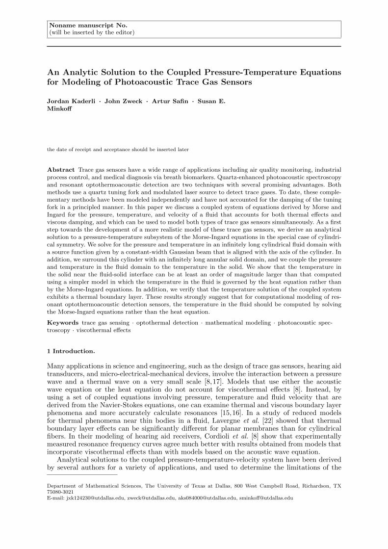
Fig. 1 Schematic diagram of a QEPAS sensor (left) and a ROTADE sensor (right). Each figure shows the quartz tuningfork (mustard) and laser source (pink).

At low ambient pressure, the same tuning fork can act as both a QEPAS sensor and aROTADE sensor. In this situation the placement of the laser beam relative to the tuning forkdictates which sensing modality is dominant. When the laser is directed near the top of the tinesof the tuning fork the QEPAS signal is dominant (see Figure 1, left), whereas when the laserbeam is directed near the base of the tuning fork the ROTADE signal is dominant (see Figure 1,right). Laboratory experiments suggest that as the laser source is moved down from the topof the tuning fork to its base, at some point the QEPAS and ROTADE signals destructivelyinterfere with one another [20,36].

QEPAS and ROTADE sensors have several promising advantages over traditional trace gassensors, including their small size (1000 times smaller than traditional sensors), immunity to en-vironmental noise, and improved sensitivity [20,23,38]. The high degree of sensitivity of QEPASand ROTADE sensors is primarily due to the very strong resonances of tuning fork oscillators.In general for an oscillator, smaller damping effects result in larger resonance amplitudes andnarrower resonance frequency widths. Physically realistic modeling of damping is therefore crit-ical for accurate computational modeling of QEPAS and ROTADE sensors [12]. In particular,since the overall damping effect depends on the geometric configuration of the system, suchmodels need to allow for the geometry of the tuning fork to be varied. Firebaugh et al. [12,13] obtained reasonable agreement between a computational model and experimental data ina study comparing the performance characteristics of several different tuning fork geometriesfor a QEPAS sensor. Previous work with a simplified model of a ROTADE sensor by Petraet al. [36] demonstrated that computer simulations can be used to optimize the tuning forkgeometry in an efficient manner. However, ad-hoc damping models were used in all these stud-ies. For example, Petra et al. [35,36] incorporated an ad-hoc damping term into the equationsdescribing the resonant vibration of the tuning fork, in which the damping constant was fittedto experimentally measured data from a single tuning fork.

The major source of damping in tuning fork oscillators is viscous damping due to the motionof the oscillator through the ambient fluid [30]. Kokubun et al. [18] developed a theoreticalmodel of the viscous damping of a tuning fork in which the drag force is calculated using fluidmechanics. By approximating a tuning fork by a string of spherical beads, they were able toapply an analytical formula for the drag force on a sphere [21] to approximate the drag forceon a vibrating tuning fork.1 However, because of its ad-hoc nature, Kokubun et al. used acurve fitting algorithm to determine the radius of the sphere in the model using data obtainedfrom experimental measurements of specific tuning forks. Firebaugh et al. [12,13] obtained

1 These formulae were obtained by solving the incompressible linear Navier-Stokes equation for viscous fluid flow arounda sphere.

4 J. Kaderli et al.

qualitative—though not quantitative—agreement with experiments using a finite-element modelof a QEPAS sensor that incorporated viscous damping of the tuning fork using the approachof Kokubun et al. They attributed the lack of quantitative agreement to the oscillating sphereapproximation used to model the viscous damping of the tuning fork.

In this paper, we take the first step towards the development of a joint mathematical modelfor QEPAS and ROTADE phenomena that more accurately incorporates viscous damping andthermal conduction effects. This new model will in the future allow for numerical optimizationof the geometric parameters of the tuning fork in these sensors. Viscous and thermal effectsin an acoustic fluid play a significant role only near the boundaries of the fluid. For harmonicplane waves, the thickness of the viscous and thermal boundary layers are each on the order of10 µm at the 32.8 kHz operating frequency of the sensor [29]. By comparison, depending on thedesign of the system, the smallest characteristic length of the geometric domain ranges from 30-100 µm [10]. Because the thickness of the boundary layers is within an order of magnitude of thesmallest characteristic length of the geometric domain, rather than treating the boundary layerseparately [3], we instead use a modification of the classical equations for acoustic pressure andheat conduction in the entire fluid domain that correctly accounts for thermal and viscous effects.This modification was obtained by Morse and Ingard [29], who linearized the Navier Stokesequations to derive a coupled system of linear partial differential equations for the acousticpressure, temperature, and fluid velocity that includes the effects of fluid viscosity and thermalconduction. By decoupling the equations for the fluid velocity from those for the other twovariables, they obtained a pair of equations for the pressure and temperature. The pressureand temperature equations are coupled to each other through a term that involves the viscosityand thermal conduction parameters of the fluid. In this paper, we add a source term to thetemperature equation which enables us to model the generation of the thermal diffusion waveand its conversion to an acoustic pressure wave in photoacoustic spectroscopy and resonantoptothermoacoustic trace gas sensors [28].

As a first step towards our goal of developing a realistic model of the coupled thermal andpressure waves, in this paper we derive an analytical solution to the Morse-Ingard equations forpressure and temperature in the special case of cylindrical symmetry. Specifically, the simplifiedsituation we consider is to solve the Morse-Ingard equations in an infinitely long cylindricalfluid domain with a source function given by a constant-width Gaussian beam that is alignedwith the axis of the cylinder. Furthermore, we surround this cylinder with an infinitely longannular solid domain, and we couple the pressure and temperature in the fluid domain to thetemperature in the solid, which we model using the heat equation. Because of the symmetriesinherent in this simplified problem, the solutions of the coupled system are functions only ofthe radial distance from the axis of the cylinder. In particular, the analytical solution we derivedoes not capture any variations of pressure and temperature along the axis of the cylinder. Wewill use the resulting solution to gain insight into how the thermal boundary layer in the fluidaffects the temperature variation in the solid near the fluid-solid interface. We show that boththe pressure and temperature variations in the fluid are the sum of a small scale thermal modeand a large scale acoustic mode. For the pressure, we show that the acoustic mode dominatesover the thermal mode. However, we will show that the temperature in the solid near the fluid-solid interface can be at least an order of magnitude larger than that computed using a simplermodel in which the temperature in the fluid is governed by the heat equation rather than bythe Morse-Ingard equations.

Globally, the geometry of a tuning fork is very different from the geometry of an infinitelylong annular domain. However, experiments and simulations have shown that the performanceof a ROTADE sensor is to a large extent determined by the temperature in that region of thetuning fork that is closest to the laser beam [34,36]. Moreover, in a ROTADE sensor, the laserbeam is positioned close to the U-shaped surface near the base of the tines of the tuning fork,and this surface is locally well approximated by the boundary of a half-cylinder (see Figure 1,right). In laboratory experiments of ROTADE sensors, the acoustic pressure of the fluid isnot resonant. Rather, the frequency of the source is chosen to excite a mechanical resonancein the tuning fork. Similarly, although the cylindrical fluid domain of the simplified system isenclosed by the solid, the frequency of the source does not excite an acoustical resonance in theradial direction. Nevertheless, since the pressure variation decays slowly it depends on the globalgeometry of the system. In summary, although the global geometry of the simplified system isdifferent from that of a trace gas sensor system, the local similarities between the two systems


are strong enough that our conclusions about the temperature in the solid should carry overto ROTADE sensors. In particular, our results strongly indicate the necessity of modeling thetemperature in the fluid using the Morse-Ingard equations, rather than using the heat equation.Indeed, in our previous modeling of ROTADE sensors that was based on the heat equation inthe fluid, we could only obtain agreement between normalized signal amplitudes rather thanbetween the amplitudes themselves [36]. While there are several factors that could contributeto this lack of agreement, the discrepancy between the results obtained using the Morse-Ingardequation and the heat equation in the fluid is likely one of them.

In Section 2 we briefly review the derivation of the Morse-Ingard equations. In Section 3we derive an analytic solution of these equations. In Section 4 we describe the finite-elementcomputation we performed to verify the correctness of the analytic solution. In Section 5 wepresent the results we obtained using both the analytical solution and finite-element method.Finally, in Section 6 we summarize the results and discuss future work.

2 Model.

In previous work, Petra et al. [34–37] developed separate models for QEPAS and ROTADEsensors. In the case of a QEPAS sensor, in which a pressure wave generates the electrical signal,Petra et al. used the acoustic wave equation to model wave propagation [35]. Similarly, inthe case of a ROTADE sensor, in which periodic thermal expansion generates the electricalsignal, they used the heat equation to describe the diffusion of the gas [36]. In this paper,we simultaneously model the temperature and pressure in an acoustic fluid using a coupledsystem of equations derived by Morse and Ingard [29, p. 279-282]. These equations are obtainedfrom a system of equations for pressure, temperature, and fluid velocity that was independentlyobtained by Morse and Ingard [29], Miklos, Shafer and Hess [28], and Joly et al. [16].

We consider a fluid that in the absence of a heat source has uniform density, pressure, andtemperature, and is everywhere at rest. When heat energy is introduced into the fluid, forexample by the interaction between a laser and a trace gas, the thermodynamic quantities varyfrom their ambient values. To derive equations for the variation of pressure, temperature, andvelocity we begin by considering the linearized Navier-Stokes equations,

ρ0∂v

∂t= −∇P +

(η +

1

3µ

)∇ (∇ · v) + µ∇ (∇ · v)− µ (∇× (∇× v)) , (1)

where v is the fluid velocity, ρ0 is ambient density, t is time, P is the variation from the ambientpressure, and µ and η are the viscosity and bulk viscosity of the fluid, respectively. By theHelmholtz Decomposition Theorem, we can express the fluid velocity in the form v = v` + vtwhere the lamellar part, v`, is curl free and the rotational part, vt, is divergence free.2 Because∇P is also curl free, we can use this decomposition to obtain separate equations for the lamellarand rotational parts:

ρ0∂v`∂t

= −∇P +

(η +

4

3µ

)∇ (∇ · v`) , (2)

ρ0∂vt∂t

= −µ (∇× (∇× vt)) . (3)

In addition to the Navier-Stokes equations, we consider the continuity of mass flow equation,

∂ρ

∂t+ ρ0∇ · v = 0, (4)

where ρ is the variation of the ambient density, ρ0, and the continuity of heat flow equation,

T0∂ζ

∂t= K∇2T , (5)

2 A theorem in the text of Chorin and Marsden [7] states that for a vector field, v, on a domain Ω ⊂ R3, the Helmholtzdecomposition, v = v` + vt, is unique, provided that we also assume that vt is tangential to the boundary surface, ∂Ω.

6 J. Kaderli et al.

where T is the variation from the ambient temperature, T0, ζ is the variation of the entropy,and K is the thermal conductivity. We also consider the equation of state,

ρ = γρ0κS (P − αT ) , (6)

where γ is the ratio of specific heats and κS is the adiabatic compressibility. In addition, theparameter, α, is given by α = ρ0βc

2/γ, where c is the speed of sound and β is the coefficient ofthermal expansion of the fluid. Finally, the equation for the variation of the entropy is given by

ζ =CpT0

(T − γ − 1

αγP), (7)

where Cp is the specific isobaric heat capacity of the fluid. Equations (2)–(7) form a system ofsix equations for the fluid velocity and the variations in the pressure, temperature, density, andentropy. Eliminating ζ and ρ from Equations (4)–(7) and focusing on the temperature variation,T , and pressure variation, P, of the fluid, we obtain:

∂

∂t

(T − γ − 1

γαP)− lhc∇2T = S, (8)

γ

c2

(∂2

∂t2− lvc

∂

∂t∇2

)(P − αT )−∇2P = 0, (9)

ρ0∂v`∂t

= −∇[P +

γlvc

∂

∂t(P − αT )

], (10)

where S = S (x, t) is the amount of heat per unit time provided by the source, t is time, andx is position. We added the source term, S, to Equation (8) to model the heating of the fluid

by the laser [16,28]. The parameter lv =(

43 + η

µ

)µρ0c

is the viscous characteristic length, and

lh = K/ρ0cCp is the thermal characteristic length. We refer to Equations (3) and (8)–(10) asthe Morse-Ingard equations. Equations (8) and (9), which are independent of the fluid velocity,v, can be solved as a system of two equations to determine the temperature and pressurevariations. In this paper we focus on Equations (8) and (9), since the tuning fork in a trace gassensor is designed to detect the pressure and temperature variations. For a tuning fork sensor,it is only necessary to solve for the fluid velocity in situations where the damping of the tuningfork cannot be obtained from experimental measurements. However, in future computationalmodels we will also include Equations (3) and (10) for the fluid velocity. The fluid velocity isneeded to impose the conditions at the interface between the fluid and tuning fork that arerequired to compute the effect of the viscous damping of the tuning fork by the fluid.

Since the tuning forks used in QEPAS and ROTADE sensors are sharply resonant, it isreasonable to assume that the source, S, is harmonic in time [35]. Consequently, we model thesource as an axially symmetric Gaussian beam of width σ of the form

S (r, t) = <C exp

[−r2/

(2σ2)]

exp(−iωt), (11)

where r is radial distance from the axis of the laser beam and <(z) denotes the real part ofa complex number, z. The angular frequency, ω, is given by ω = 2πf , where f is the wavefrequency. This frequency is chosen to match the resonance frequency of the tuning fork, whichis typically f = 32.8 kHz. The parameter, C, is given by C = αeffWL/

(4πρ0Cpσ

2)

where αeff isthe effective absorption coefficient (i.e., the fraction of radiation absorbed per unit length as itpasses through fluid), and WL is the laser power [35].

To enable us to derive cylindrically symmetric solutions, we solve the Morse-Ingard Equa-tions (8) and (9) with a source function given by Equation (11) in an infinitely long cylindricalfluid domain, Ωfluid, of radius, R, that is aligned with the axis of the laser beam. Furthermore,we couple the pressure and temperature variations in the fluid to the temperature variationin an infinitely long annular solid domain, Ωsolid, surrounding the fluid with inner radius, R,and outer radius, RS . We show a cross section of the composite domain, Ω = Ωfluid ∪Ωsolid inFigure 2.

We will use the resulting analytical solution to gain insight into how the thermal boundarylayer in the fluid affects the temperature variation in the solid near the fluid-solid interface.


We anticipate that the behavior of the temperature variation in the solid near the fluid-solidinterface obtained on the simplified geometric domain will be similar to that in the tuning forkof a ROTADE sensor. In particular, experiments have shown that that the performance of aROTADE sensor is to a large extent determined by the temperature in that region of the tuningfork that is closest to the laser beam [34,36]. Moreover, since the laser beam is positioned closeto the U-shaped surface near the base of the tuning fork, locally in this region, the boundary iswell approximated by the boundary of a half-cylinder (see Figure 1, right).

RS

R

Fig. 2 Cross section of a cylindrical fluid domain of radius, R, surrounded by an annular solid domain with outer radius,RS .

Because of the cylindrical symmetry of the both source function, S, and the compositedomain, Ω = Ωfluid ∪ Ωsolid, the temperature and pressure variations are functions only of theradial distance, r, from the axis of the laser beam. Moreover, since we are only interested intime-harmonic, steady-state solutions, we can express the pressure, temperature, and source inthe form

P (r, t) = <P (r) e−iωt

, T (r, t) = <

T (r) e−iωt

, S (r, t) = <

S (r) e−iωt

. (12)

Under these assumptions, the coupled system of time-dependent partial differential equations (8)and (9) reduces to the coupled Helmholtz system of second-order ordinary differential equations,

lhc∇2T + iω

(T − γ − 1

γαP

)= −S, (13)

∇2P +γ

c2

(ω2 − ilvcω∇2

)(P − αT ) = 0, (14)

where the Laplacian operator of a function, F = F (r), is given by ∇2F = F ′′ + 1rF′. Here

F ′ = dF/dr.The temperature, TS , in the solid, Ωsolid, satisfies the heat equation

∂TS∂t−DS∇2TS = 0, (15)

where DS is the thermal diffusivity of the solid. Assuming a time-harmonic solution, we havethat TS(r, t) = <TS (r) e−iωt and so the Helmholtz form of Equation (15) is

T ′′S +1

rT ′S +

iω

DSTS = 0, (16)

which has the solutionTS (r) = d1J0 (kr) + d2H

(1)0 (kr) . (17)

8 J. Kaderli et al.

Here k =√

iωDS

and J0 is the zeroth order Bessel function of the first kind and H(1)0 is the zeroth

order Hankel function of the first kind [32]. We express the solution using this particular linear

combination because J0 and H(1)0 form a numerically satisfactory pair of cylinder functions in

the upper half of the complex plane [32, 10.2(iii)].In Section 3, we will derive a formula for the general solution of Equations (13) and (14) in

terms of Bessel and Hankel functions. Because these equations are both of second order, thegeneral solution will have four unknown constants. In addition, the temperature solution in theannulus given by Equation (17) has two unknown constants, d1 and d2. To determine these sixconstants we impose the six conditions,

T (0) <∞, (18)

P (0) <∞, (19)

T (R) = TS (R) , (20)

KF∇T (R) = KS∇TS (R) , (21)

P ′ (R) = 0, (22)

TS (RS) = 0, (23)

where KF and KS are the thermal conductivities of the fluid and solid, respectively. The first twoconditions are necessary to guarantee that the solution is bounded, since the Hankel functionshave a singularity at zero. The third and fourth conditions ensure continuity of temperature andheat flux across the fluid-solid interface. The fifth condition ensures that the normal derivativeof the pressure is zero at the fluid-solid interface. To a first approximation, this assumption isreasonable when modeling the acoustic pressure in a trace gas sensor that employs a tuningfork, since the amplitude of vibration of the tuning fork is several orders of magnitude smallerthan the characteristic lengths of the system. Therefore, it is reasonable to also assume that thesurface of the annular solid in our simplified model is rigid. The sixth condition states that thetemperature variation is zero on the outer wall of the annulus. This assumption is reasonablesince the temperature variation is known to decay exponentially in the solid, and because weare most interested in computing the temperature near the inner wall of the annulus.

Imposing the condition T (R) = 0 in place of conditions (20), (21), and (23) yields essentiallythe same solution in the fluid. However, in future work, we will develop a model for a trace gassensor in which the pressure and temperature in the fluid and the temperature in the tuningfork are coupled to the mechanical deformation of the tuning fork. For this model, setting thetemperature to zero on the boundary of the tuning fork would be incorrect as laboratory datahas shown that at low ambient pressure the output of the sensor depends on both the pressurevariation at the interface and the temperature variation in the tuning fork near the interface.One of our goals in this paper is to determine whether it is necessary to use the coupled systemgiven by Equations (13) and (14) to model the pressure and temperature in the fluid, or whetherit is sufficient to separately compute solutions of the acoustic wave and heat equations. Sincethis question cannot be answered by imposing the condition T (R) = 0, we instead use the morerealistic conditions (20), (21), and (23).

3 Derivation of the Analytic Solution.

To solve Equations (13) and (14), we adapt the method used by Petra et al. [35] who employedthe acoustic wave equation to model the propagation of pressure waves in a QEPAS sensor.By considering the Helmholtz form of the equation Petra and coauthors were able to use themethod of variation of parameters to derive an analytic solution to the acoustic wave equationin terms of Bessel and Hankel functions. In this section, we use a similar approach to solve theMorse-Ingard equations.

To facilitate the derivation of the solution and to focus attention on the parameters ofinterest, we nondimensionalize the Morse-Ingard equations using the nondimensional quantities

x∗ =ωx

c, ∇∗ =

c

ω∇, P∗ = P

(cx∗ω

), T∗ = αT

(cx∗ω

),

S∗ = −αωS(cx∗ω

), Ω =

ωlhc, and Λ =

ωlvc. (24)


Substituting these nondimensionalized quantities into Equations (13) and (14) gives

Ω∇2∗T∗ + iT∗ − i

γ − 1

γP∗ = S∗, (25)

∇2∗P∗ + γ

(1− iΛ∇2

∗)

(P∗ − T∗) = 0. (26)

To eliminate the spatial derivative of temperature in Equation (26), we substitute Equation(25) into Equation (26) to obtain the new system,

Ω∇2T + iT − iγ − 1

γP = S, (27)

(1− iγΛ)∇2P +

[γ

(1− Λ

Ω

)+Λ

Ω

]P − γ

(1− Λ

Ω

)T = −iγ Λ

ΩS. (28)

Here we have dropped the star notation. However, the reader should keep in mind that we areworking with nondimensionalized quantities for the remainder of Section 3. Note that while theequations are still coupled, each has derivatives of temperature or pressure only. Thus we canwrite Equations (27) and (28) as

Ω

(T ′′ +

1

rT ′)

+ iT − iγ − 1

γP = S, (29)

(1− iγΛ)

(P ′′ +

1

rP ′)

+

[γ

(1− Λ

Ω

)+Λ

Ω

]P − γ

(1− Λ

Ω

)T = −iγ Λ

ΩS. (30)

3.1 Solution of the Homogeneous Equations.

We begin by finding the solution of the homogeneous version of the system (29) and (30). WhenS = 0, solving Equation (29) for P gives

P =γ

γ − 1

[T − iΩ

(T ′′ +

1

rT ′)]

. (31)

Because of the presence of the Laplacian in cylindrical coordinates in Equation (31), it is naturalto suppose that T = C0 (kr), where C0 is a cylinder function of order zero, i.e., a linear combi-nation of Bessel and Hankel functions of order zero [32], and k is a constant to be determined.Consequently, T satisfies T ′′ + 1

rT′ = −k2T , and so Equation (31) can be rewritten as

P = mT = mC0 (kr) where m =γ

γ − 1

(1 + iΩk2

). (32)

Since P is also a cylinder function, Equation (30) reduces to the algebraic equation

(1− iγΛ)(−k2P

)+

[γ

(1− Λ

Ω

)+Λ

Ω

]P − γ

(1− Λ

Ω

)T = 0. (33)

Since P = mT , and assuming T is not identically zero, we conclude that

(iΩ + γΩΛ) k4 + (1− iγΩ − iΛ) k2 − 1 = 0. (34)

Therefore, for T = C0 (kr) and P = mC0 (kr) to be solutions of the homogeneous equations (29)and (30), the parameter k must be a solution of Equation (34). Consequently,

k2 =i

2Ω

(1− iγΩ − iΛ±Q

1− iγΛ

), (35)

whereQ2 = (1− iγΩ − iΛ)2 + 4 (iΩ + γΩΛ) . (36)

10 J. Kaderli et al.

Next we define

k2t =

i

2Ω

(1− iγΩ − iΛ+Q

1− iγΛ

)and k2

p =i

2Ω

(1− iγΩ − iΛ−Q

1− iγΛ

), (37)

and setmt =

γ

γ − 1

(1 + iΩk2

t

)and mp =

γ

γ − 1

(1 + iΩk2

p

). (38)

We note that Equation (37) also holds for plane and spherical harmonic waves [6,29]. Theconstants kp and kt correspond to acoustic and thermal modes, respectively [29]. The acousticmode has a small imaginary part and attenuates slowly whereas the thermal mode has both a

large real and large imaginary part and attenuates rapidly. Because J0 andH(1)0 are a numerically

satisfactory pair of cylinder functions in the upper half of the complex plane [32, 10.2(iii)], weuse them to obtain the fundamental set of solutions to the homogeneous equations (29) and(30): [

T (r)P (r)

]∈

[J0 (kpr)

mpJ0 (kpr)

],

[H

(1)0 (kpr)

mpH(1)0 (kpr)

],

[J0 (ktr)mtJ0 (ktr)

],

[H

(1)0 (ktr)

mtH(1)0 (ktr)

]. (39)

3.2 Solution of the Inhomogeneous Equations.

Having found a fundamental set of solutions (39) to the homogeneous version of Equations (29)and (30), we now solve the inhomogeneous equations (29) and (30). Introducing new variablesfor T ′ and P ′, we can rewrite the two second order equations (29) and (30) as the first ordersystem

u′ (r) =M (r)u (r) + g (r) , (40)

where

u (r) =

T (r)T ′ (r)P (r)P ′ (r)

M (r) =

0 1 0 0

− iΩ −1

ri(γ−1)γΩ 0

0 0 0 1γ(1− Λ

Ω )1−iγΛ 0

γ(1− ΛΩ )+ Λ

Ω

1−iγΛ −1r

g (r) =

0

1ΩS (r)

0

− iγΛΩ(1−iγΛ)S (r)

. (41)

Using the method of variation of parameters [4], the solution of the inhomogeneous system (40)can be written as

u (r) = Ψ (r)

(b +

∫ r

0Ψ−1 (s)g (s) ds

), (42)

where b is a constant of integration and Ψ is the fundamental matrix

Ψ (r) =

J0 (kpr) H

(1)0 (kpr) J0 (ktr) H

(1)0 (ktr)

−kpJ1 (kpr) −kpH(1)1 (kpr) −ktJ1 (ktr) −ktH(1)

1 (ktr)

mpJ0 (kpr) mpH(1)0 (kpr) mtJ0 (ktr) mtH

(1)0 (ktr)

−kpmpJ1 (kpr) −kpmpH(1)1 (kpr) −ktmtJ1 (ktr) −ktmtH

(1)1 (ktr)

. (43)

We use the Schur complement [26] to calculate Ψ−1. Specifically, we employ the blocking

Ψ =

[A BC D

], (44)

where

A =

[J0 (kpr) H

(1)0 (kpr)

−kpJ1 (kpr) −kpH(1)1 (kpr)

], B =

[J0 (ktr) H

(1)0 (ktr)

−ktJ1 (ktr) −ktH(1)1 (ktr)

], (45)

andC = mpA and D = mtB. (46)


Then

Ψ−1 =

[A BC D

]−1

=

[S−1 −S−1BD−1

−D−1CS−1 D−1 +D−1CS−1BD−1

], (47)

whereS = A− BD−1C. (48)

Substituting D−1 = 1mtB−1 and Equations (46) into Equation (48) yields

S =mt −mp

mtA. (49)

Therefore

Ψ−1 =1

mt −mp

[mtA−1 −A−1

−mpB−1 B−1

], (50)

where

A−1 (r) =πr

2i

[−kpH(1)

1 (kpr) −H(1)0 (kpr)

kpJ1 (kpr) J0 (kpr)

], B−1 (r) =

πr

2i

[−ktH(1)

1 (ktr) −H(1)0 (ktr)

ktJ1 (ktr) J0 (ktr)

].

To calculate A−1 and B−1 we used the property that W(J0 (z) , H

(1)0 (z)

)= 2i/ (πz) where W

denotes the Wronskian [32]. Thus the inverse of the fundamental matrix is given by

Ψ−1 (r) =πr

2i (mt −mp)

−kpmtH

(1)1 (kpr) −mtH

(1)0 (kpr) kpH

(1)1 (kpr) H

(1)0 (kpr)

kpmtJ1 (kpr) mtJ0 (kpr) −kpJ1 (kpr) −J0 (kpr)

ktmpH(1)1 (ktr) mpH

(1)0 (ktr) −ktH(1)

1 (ktr) −H(1)0 (ktr)

−ktmpJ1 (ktr) −mpJ0 (ktr) ktJ1 (ktr) J0 (ktr)

. (51)

Applying the variation of parameters formula (42) we conclude that the general solution ofthe first order system (40) is

u (r) = Ψ (r) (b + c (r)) . (52)

Here, b = [b1, b2, b3, b4]T is a vector of unknown constants and c (r) = [c1 (r) , c2 (r) , c3 (r) , c4 (r)]T

where

c1 (r) =π

2i (mt −mp)

(E − mt

Ω

)∫ r

0sH

(1)0 (kps)S (s) ds, (53)

c2 (r) = − π

2i (mt −mp)

(E − mt

Ω

)∫ r

0sJ0 (kps)S (s) ds, (54)

c3 (r) = − π

2i (mt −mp)

(E − mp

Ω

)∫ r

0sH

(1)0 (kts)S (s) ds, (55)

c4 (r) =π

2i (mt −mp)

(E − mp

Ω

)∫ r

0sJ0 (kts)S (s) ds, (56)

and E = −iγΛ/ (Ω (1− iγΛ)). From the first and third rows of Equation (52), we conclude thatthe general solution of the inhomogeneous system (29) and (30) is given by

T (r) = (b1 + c1 (r)) J0 (kpr) + (b2 + c2 (r))H(1)0 (kpr) +

(b3 + c3 (r)) J0 (ktr) + (b4 + c4 (r))H(1)0 (ktr) , (57)

P (r) = (b1 + c1 (r))mpJ0 (kpr) + (b2 + c2 (r))mpH(1)0 (kpr) +

(b3 + c3 (r))mtJ0 (ktr) + (b4 + c4 (r))mtH(1)0 (ktr) . (58)

To determine the constants b1, b2, b3, and b4 in Equations (57) and (58), as well as the constantsd1 and d2 in Equation (17), we use boundary conditions (18)–(23). To apply the first condition

(18), we consider limr→0

T (r) in Equation (57). By using the approximation H(1)0 (r) ≈ (2i/π) ln (r)


[32], which is valid for small r, along with repeated application of L’Hopital’s Rule, we concludethat condition (18) gives

b2 + b4 = 0. (59)

Similarly, by considering limr→0

P (r), we conclude that condition (19) gives

b2mp + b4mt = 0. (60)

Therefore, since mp 6= mt, Equations (59) and (60) imply

b2 = b4 = 0. (61)

Thus the coupled solution given in Equation (57) and (58) simplifies to

T (r) = (b1 + c1 (r)) J0 (kpr) + c2 (r)H(1)0 (kpr) +

(b3 + c3 (r)) J0 (ktr) + c4 (r)H(1)0 (ktr) , (62)

P (r) = (b1 + c1 (r))mpJ0 (kpr) + c2 (r)mpH(1)0 (kpr) +

(b3 + c3 (r))mtJ0 (ktr) + c4 (r)mtH(1)0 (ktr) . (63)

Using Equations (62) and (63) and the four boundary conditions (20)–(23), we obtain thelinear system of four equations in four unknown constants b1, b3, d1, and d2 given by

J0 (kpR) J0 (ktR) −J0 (kR) −H(1)0 (kR)

kpJ1 (kpR) ktJ1 (ktR) −KSKF

kJ1 (kR) −KSKF

kH(1)1 (kR)

mpkpJ1 (kpR) mtktJ1 (ktR) 0 0

0 0 J0 (kRS) H(1)0 (kRS)

b1b3d1

d2

=

F1

F2

F3

0

, (64)

where

F1 = −c1 (R) J0 (kpR)− c2 (R)H(1)0 (kpR)− c3 (R) J0 (ktR)− c4 (R)H

(1)0 (ktR) , (65)

F2 = −kpc1 (R) J1 (kpR)− kpc2 (R)H(1)1 (kpR)− ktc3 (R) J1 (ktR)− ktc4 (R)H

(1)1 (ktR) , (66)

F3 = −mpkpc1 (R) J1 (kpR)−mpkpc2 (R)H(1)1 (kpR)−

mtktc3 (R) J1 (ktR)−mtktc4 (R)H(1)1 (ktR) . (67)

Solving the third row for b3 and the fourth row for d2 and then substituting these expressionsinto the two other rows we can reduce the system (64) to the 2 × 2 system

J0 (kpR)− mpkpJ1(kpR)J0(ktR)mtktJ1(ktR)

J0(kRS)H(1)0 (kR)

H(1)0 (kRS)

− J0 (kR)

kpJ1 (kpR)(

1− mpmt

)KSkKF

(J0(kRS)H

(1)1 (kR)

H(1)0 (kRS)

− J1 (kR)

)[ b1d1

]=

[F1 − J0(ktR)F3

mtktJ1(ktR)

F2 − F3mt

].

(68)The 2 × 2 system (68) can now be solved for b1 and d1, and using those values in the 4 × 4

system (64), we can find b3 and d2. We now have a complete solution to the coupled temperatureand pressure system given by Equations (62) and (63). At this point, we remind the reader thatall quantities in these equations are nondimensional, but that they can be converted back tophysical units using Equation (24).


4 Finite-Element Computation of the Solution.

As an additional check, we compared the analytical solution derived in the previous sectionto a finite element solution computed on the two-dimensional domain shown in Figure 2. Ourfinite element implementation, which was developed using the FEniCS package [24], is a firststep towards a computational model for QEPAS and ROTADE sensors in three dimensionswith realistic geometry. One of our major motivations for deriving the cylindrically symmetricanalytical solution is that it can be used to help verify the correctness of such a computationalmodel.

For the finite-element results in this paper, we solved the coupled Helmholtz system consist-ing of the the Morse-Ingard equations (13) and (14) in a disk-shaped fluid domain, Ωfluid, andthe heat equation (15) in an annular solid domain, Ωsolid, with boundary and interfacial con-ditions given by Equations (20)–(23). Since FEniCS does not support complex arithmetic, wedecomposed the variables into real and imaginary components, T = T1 + iT2 and P = P1 + iP2,as in [5]. With this decomposition, the entries of the complex-valued finite-element matrices areconverted into 2×2 blocks of corresponding real-valued matrices. The mesh was generated usingthe Gmsh package [14]. The mesh was refined around the source and near the interface betweenthe fluid and solid subdomains (see Figure 3). For our FEniCS implementation, we used linearLagrange interpolating polynomials on triangular elements. Finally, the assembled system wassolved using the sparse LU decomposition algorithm in the PETSc package [1]. The finite el-ement system we solved had approximately 2 × 105 unknowns on a mesh with 105 triangularelements. In Figure 3 we show a slightly coarser mesh (with 104 triangular elements) which hasthe same characteristics as our simulation mesh. We note that with a finer mesh it is harderto discern the refinement around the source and at the fluid-solid interface due to the densityof the elements. For comparison with the analytical solution, we used linear interpolation tocompute the values of the temperature and pressure along the x-axis of the two-dimensionaldomain.

X

Y

Z

Fig. 3 A finite-element mesh with 104 triangular elements for the domain shown in Figure 2.

5 Numerical Results.

In this section, we numerically investigate the solution of the Morse-Ingard equations derived inSection 3. We first verify the correctness of the analytic solution for temperature and pressureby comparison to a purely numerical solution computed via the finite element method. Next,we show that the temperature solution from the Morse-Ingard equations differs significantly


from the solution obtained using the heat equation in the fluid. In particular, we show that theMorse-Ingard solution produces a thermal boundary layer which is not present in the solutionobtained using the heat equation in the fluid. This boundary layer results from the interactionof a thermal part and an acoustic part of the solution of nearly equal magnitudes.

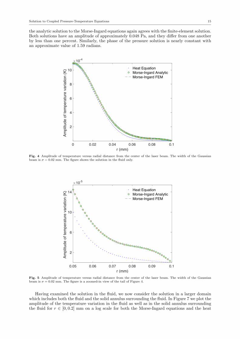
For all the numerical simulations, we assume that the fluid is nitrogen gas at a temperatureof 300 K and a pressure of 1 bar [36]. The parameter values we used are shown in Table 5.All the parameter values in the simulations closely correspond to those used in our previousmodeling of laboratory experiments of QEPAS and ROTADE sensors [35,36]. In the first setof numerical simulations, we assume that the width of the Gaussian source σ is 0.02 mm. InFigure 4 we show the amplitude of the temperature variation in the fluid as a function of theradial distance, r, from the center of the laser beam over the interval [0, 0.1] mm. The threecurves show the solution to the heat equation in the fluid (dots), the analytic solution of theMorse-Ingard equations (circles), and the solution of the Morse-Ingard equations via the finite-element method (dashes). The analytic solution of the Morse-Ingard equations agrees with thefinite-element solution, thus verifying the accuracy of both solution methods. Also, in Figure 4,we see the amplitudes of the temperature variation given by the Morse-Ingard equations andthe heat equation in the fluid agree well for r ∈ [0, 0.025] mm. However, as r increases, thetwo amplitudes diverge, as is seen more clearly in Figure 5, which shows the same solutionsas Figure 4 over the interval [0.05, 0.1] mm rather than over the full interval [0, 0.1] mm. Thesolutions of the heat equation and the Morse-Ingard equations disagree in this region. Forexample, at r = 0.08 mm, we see that the amplitude of the temperature given by the Morse-Ingard equations

(≈ 3.3× 10−5 K

)is about four times the amplitude of the temperature given

by the heat equation(≈ 7.7× 10−6 K

).

Source Frequency f = 3.28× 104 HzSource Width σ = 2× 10−5 m or 1× 10−6 m

Radius of Nitrogen Gas Domain R = 1× 10−4 mOuter Radius of Solid Annulus RS = 2× 10−4 m

Thermal Conductivity of Nitrogen Gas KF = 0.0259 W m−1 K−1

Density of Nitrogen Gas ρ0 = 1.123 kg m−3

Specific Isobaric Heat Capacity of Nitrogen Gas Cp = 1041 J kg−1 K−1

Ratio of Specific Heats of Nitrogen Gas γ = 1.4Thermal Expansion of Nitrogen Gas β = 3.33× 10−3 K−1

Bulk (Volume) Viscosity of Nitrogen Gas η = 1.3× 10−5 kg m−1 s−1

Viscosity of Nitrogen Gas µ = 1.76× 10−5 kg m−1 s−1

Speed of Sound in Nitrogen Gas c = 353 m s−1

Thermal Conductivity of Solid KS = 16 W m−1 K−1

Thermal Diffusivity of Solid DS = 4× 10−6 m2 s−1

Effective Absorption Coefficient αeff = 0.05 m−1

Laser Power WL = 3× 10−2 WThermal Characteristic Length lh = 6.276× 10−8 mViscous Characteristic Length lv = 9.199× 10−8 m

— α = ρ0βc2

γ = 333.18 kg m−1 K−1 s−2

Table 1 Parameters used in the numerical simulations.

In Figure 6 we plot the phase of the temperature variation relative to the source as a functionof r over the interval [0, 0.1] mm. (We assume that the phase of the source is zero, see Equa-tion (11).) Once again, we observe excellent agreement between the analytical and numericalsolutions of the Morse-Ingard equations. However, although the phase of the temperature solu-tions of the Morse-Ingard equations and of the heat equation in the fluid agree well for small r,they differ significantly as r increases.

The pressure solution of the Morse-Ingard equations is dominated by the acoustic mode,which attenuates very slowly, and is therefore nearly constant over the interval [0, 0.1] mm.While we do not include plots of the amplitude or phase of the pressure variation in this paper,


the analytic solution to the Morse-Ingard equations again agrees with the finite-element solution.Both solutions have an amplitude of approximately 0.048 Pa, and they differ from one anotherby less than one percent. Similarly, the phase of the pressure solution is nearly constant withan approximate value of 1.59 radians.

0 0.02 0.04 0.06 0.08 0.1r (mm)

2

4

6

8

10Am

plitu

de o

f tem

pera

ture

var

iatio

n (K

)×10-4

Heat EquationMorse-Ingard AnalyticMorse-Ingard FEM

Fig. 4 Amplitude of temperature versus radial distance from the center of the laser beam. The width of the Gaussianbeam is σ = 0.02 mm. The figure shows the solution in the fluid only.

0.05 0.06 0.07 0.08 0.09 0.1r (mm)

2

6

10

14

Ampl

itude

of t

empe

ratu

re v

aria

tion

(K)

×10-5


Fig. 5 Amplitude of temperature versus radial distance from the center of the laser beam. The width of the Gaussianbeam is σ = 0.02 mm. The figure is a zoomed-in view of the tail of Figure 4.

Having examined the solution in the fluid, we now consider the solution in a larger domainwhich includes both the fluid and the solid annulus surrounding the fluid. In Figure 7 we plot theamplitude of the temperature variation in the fluid as well as in the solid annulus surroundingthe fluid for r ∈ [0, 0.2] mm on a log scale for both the Morse-Ingard equations and the heat


0 0.02 0.04 0.06 0.08 0.1r (mm)

0

π/2

π

3π/2

Phas

e of

tem

pera

ture

var

iatio

n (ra

d)


Fig. 6 Phase of temperature versus radial distance from the center of the laser beam. The width of the Gaussian beam isσ = 0.02 mm. The figure shows the solution in the fluid only.

equation in the fluid. The width of the laser source is still σ = 0.02 mm, and the fluid-structureinterface is located at r = 0.1 mm. At the interface, the temperature solution to the Morse-Ingard equations is between one and two orders of magnitude larger than the solution obtainedusing the heat equation in the fluid. Since the amplitude of vibration of the quartz tuning fork ina ROTADE sensor is primarily determined by the temperature variation at the fluid-structureinterface [36], this result strongly indicates that the solution of the heat equation in the fluidis likely to be a poor approximation when modeling thermal effects in trace gas sensors. Inparticular, since the signal-to-noise ratio in a tuning fork sensor is approximately 1000, (i.e.,30 dB) [11], ROTADE sensors can readily distinguish between temperature variations that areless than an order of magnitude apart.

0.02 0.06 0.1 0.14 0.18r (mm)

-12

-8

-4

Log

of a

mpl

itude

of t

empe

ratu

re v

aria

tion

(K)

Heat EquationMorse-Ingard Equation

Fig. 7 Semilog plot of the amplitude of the temperature variation as a function of radial distance from the center of thelaser beam. The width of the Gaussian beam is σ = 0.02 mm. The figure shows the solution in both the fluid, r ∈ [0, 0.1]mm, and the surrounding solid, r ∈ [0.1, 0.2] mm.


In the second set of numerical simulations, we assume a narrower width for the Gaussiansource, i.e., σ = 0.001 mm. In Figure 8, we show the amplitude of the temperature variationin the fluid as a function of the radial distance, r, from the center of the laser beam over theinterval [0, 0.1] mm. The two curves show the solution obtained using the heat equation in thefluid and the analytic solution of the Morse-Ingard equations. Because the source is narrower,in this case, the solution decays much faster than in the previous case, as can be seen bycomparing Figures 4 and 8. In addition, we observe a boundary layer, as shown in Figure 9. Thisfigure shows the same solutions as Figure 8 but over the smaller interval [0.05, 0.1] mm. Whilethe solution to the heat equation decreases monotonically, the solution to the Morse-Ingardequation increases for r ∈ [0.06, 0.08] mm before decreasing for r ∈ [0.08, 0.1] mm. Accordingto Morse and Ingard, for a plane harmonic wave, the width of the temperature boundary layeris√

2lhc/ω ≈ 0.0147 mm [29, p. 286]. In Figure 9, we see that for the cylindrical harmonicwave, the width of the boundary layer is approximately 0.05 mm, which is on the same orderof magnitude as that predicted by Morse and Ingard.

0 0.02 0.04 0.06 0.08 0.1r (mm)

2

6

10

Ampl

itude

of t

empe

ratu

re v

aria

tion

(K)

×10-3

Heat EquationMorse-Ingard Analytic

Fig. 8 Amplitude of the temperature variation as a function of radial distance from the center of the laser beam. Thewidth of the Gaussian beam is narrower than in Figures 4–7 with σ = 0.001 mm. The figure shows the solution in the fluidonly.

In Figure 10, we show the phase of the temperature variation as a function of r over theinterval [0, 0.1] mm. Comparing Figures 6 and 10, we also see that there is a more rapid changein phase of the temperature solution of the Morse-Ingard equations when the Gaussian beam isnarrower.

Both the thermal wave, T , and the pressure wave, P , contain a thermal part and an acousticpart. The acoustic part of the temperature solution is given by the first two terms of Equa-

tion (62), i.e., (b1 + c1 (r)) J0 (kpr) + c2 (r)H(1)0 (kpr), and the thermal part of the temper-

ature solution is given by the last two terms of Equation (62), i.e., (b3 + c3 (r)) J0 (ktr) +

c4 (r)H(1)0 (ktr). The acoustic and thermal parts of the pressure solution are given by the anal-

ogous terms of Equation (63). In Figure 11 we show the acoustic and thermal parts of thetemperature variation using the source with the narrower width of σ = 0.001 mm. For smallr, the thermal part of the solution is about two orders of magnitude larger than the acousticpart. For example, at r = 0.02 mm, the amplitude of the thermal part of the temperaturesolution (≈ 0.001 K) is about 24 times the amplitude of the acoustic part of the temperaturesolution

(≈ 4.17× 10−5 K

). As r increases, the acoustic part remains relatively constant while

the thermal part decreases. When both parts are roughly the same order of magnitude, theyproduce the variation in amplitude in the radial direction seen in Figure 9. In Figure 12, weshow the acoustic and thermal parts of the pressure variation. The acoustic part of the solution


0.05 0.06 0.07 0.08 0.09 0.1r (mm)

2

4

6

8

Ampl

itude

of t

empe

ratu

re v

aria

tion

(K)

×10-5


Fig. 9 Amplitude of the temperature variation as a function of radial distance from the center of the laser beam. Thefigure is a zoomed-in view of the tail of Figure 8. The width of the Gaussian beam is σ = 0.001 mm.

0 0.02 0.04 0.06 0.08 0.1r (mm)

0

π/2

π

3π/2

Phas

e of

tem

pera

ture

var

iatio

n (ra

d)


Fig. 10 Phase of the temperature variation as a function of radial distance from the center of the laser beam. The widthof the Gaussian beam is the same as in Figures 8 and 9 with σ = 0.001 mm. The figure shows the solution in the fluid only.

is at least two orders of magnitude larger than the thermal part of the solution. For example, atr = 0.02 mm, the amplitude of the acoustic part of the pressure solution (≈ 0.0486 Pa) is about5900 times the amplitude of the thermal part of the pressure solution

(≈ 8.27× 10−6 Pa

). As

r increases, the ratio of the amplitude of the acoustic part to the thermal part of the pres-sure solution also increases. In summary, the thermal mode dominates the temperature solutionaway from the boundary layer, while the acoustic mode dominates the pressure solution overthe entire fluid domain. For both the temperature and pressures solutions, the thermal modeattenuates rapidly as described by Morse and Ingard [29, p. 282-283].


0 0.02 0.04 0.06 0.08 0.1r (mm)

4.15

4.16

4.17

4.18Am

plitu

de o

f tem

pera

ture

var

iatio

n (K

)×10-5

(a) Acoustic part of temperature.

0 0.02 0.04 0.06 0.08 0.1r (mm)

0

0.004

0.008

0.012

Ampl

itude

of t

empe

ratu

re v

aria

tion

(K)

(b) Thermal part of temperature.

Fig. 11 Amplitude of (a) the acoustic part and (b) the thermal part of temperature variation as a function of radialdistance from the center of the laser beam. The width of the Gaussian beam is σ = 0.001 mm. The figures show thesolution in the fluid only.

0 0.02 0.04 0.06 0.08 0.1r (mm)

0.0484

0.0485

0.0486

0.0487

Ampl

itude

of p

ress

ure

varia

tion

(Pa)

(a) Acoustic part of pressure.

0 0.02 0.04 0.06 0.08 0.1r (mm)

0

0.2

0.4

0.6

0.8

1

Ampl

itude

of p

ress

ure

varia

tion

(Pa)

×10-4

(b) Thermal part of pressure.

Fig. 12 Amplitude of (a) the acoustic part and (b) the thermal part of pressure variation as a function of radial distancefrom the center of the laser beam. The width of the Gaussian beam is σ = 0.001 mm. The figures show the solution in thefluid only.

6 Conclusions.

We derived an analytic solution to the coupled system of pressure-temperature equations ofMorse and Ingard. By assuming that the laser source can be represented as a time-harmonicfunction and by using the cylindrical symmetry of the domain, we converted the partial differ-ential equations into ordinary differential equations for which the independent variable is givenby the radial distance from the center of the laser beam. We solved these ordinary differen-tial equations using the method of variation of parameters. The constants of integration werefound by solving a system of linear equations obtained from the boundary conditions. We thenverified the correctness of the analytic solution by comparing it to the solution computed viathe finite-element method. We also compared the solution of the Morse-Ingard equations to thesolution of the heat equation in the fluid and found that the coupled nature of the Morse-Ingardequations results in a significantly larger temperature variation than that predicted by the heatequation, especially in the solid near the fluid-solid interface. This discrepancy demonstratesthe importance of using the Morse-Ingard equations for more realistic computational modelingof trace gas sensors.

In addition, because the Morse-Ingard equations include parameters that model viscother-mal effects, the analytic solution we derived in this paper provides a starting point for the


development of a mathematical model of QEPAS and ROTADE sensors which accounts forthe damping of the tuning fork. The ultimate goal of such an improved model is to allow forthe efficient optimization of the tuning fork geometry via computer simulations so that the fullbenefit of this promising technology may be realized.

An important application of the analytical solution we derived is that it can be used to verifythe correctness of computational models for trace gas sensors that are based on finite-elementsolutions of the Morse-Ingard equations. In particular, because we correctly model the source,we expect the behavior of the cylindrically symmetric pressure and temperature solutions to bequalitatively similar to that in a trace gas sensor. By comparison, the plane wave solutions weused in past verification studies are qualitatively very different [5].

To quantify the performance of a QEPAS/ROTADE sensor, the Morse-Ingard equations inthe fluid need to be coupled to the system of equations for the displacement of the tuning fork.As we will show in future work, this coupling is via conditions on the interface between the fluidand tuning fork. In particular, the condition on the tuning fork due to the fluid includes a termthat involves the viscous stress tensor of the fluid and models the damping of the tuning forkdue to its motion through the viscous fluid [16]. With the recent interest in further miniaturizingthese devices, the thermal and viscous boundary layers become more significant, emphasizingthe importance of our new model [15].

References

1. Balay, S., Abhyankar, S., Adams, M.F., Brown, J., Brune, P., Buschelman, K., Dalcin, L., Eijkhout, V., Gropp,W., Kaushik, D., Knepley, M., McInnes, L., Rupp, K., Smith, B., Zampini, S., Zhang, H.: PETSc Webpage.http://www.mcs.anl.gov/petsc (2015)

2. Bell, A.: On the production and reproduction of sound by light. Am. J. Sci. 20, 305–324 (1880)3. Bossart, R., Joly, N., Bruneau, M.: Hybrid numerical and analytical solutions for acoustic boundary problems in

thermo-viscous fluids. J. Sound Vib. 263, 69–84 (2003)4. Boyce, W., DiPrima, R.: Elementary Differential Equations, 8th edn. John Wiley (2005)5. Brennan, B., Kirby, R., Zweck, J., Minkoff, S.: High-performance python-based simulations of pressure and temperature

waves in a trace gas sensor. Proceedings of PyHPC 2013: Python for High Perfomance and Scientific Computing (2013)6. Cao, Y., Diebold, G.J.: Effects of heat conduction and viscosity on photoacoustic waves from droplets. Optical Engi-

neering 36(2), 417–422 (1997)7. Chorin, A.J., Marsden, J.E.: A Mathematical Introduction to Fluid Mechanics. Springer-Verlag, New York, N.Y. (1979)8. Cordioli, J., Martins, G., Mareze, P., Jordan, R.: A comparison of models for visco-thermal acoustic problems. In:

Inter-Noise. International Institute of Noise Control Engineering (2010)9. Curl, R., Capasso, F., Gmachl, C., Kosterev, A., McManus, B., Lewicki, R., Pusharsky, M., Wysocki, G., Tittel, F.:

Quantum cascade lasers in chemical physics. Chemical Physics Letters 487, 1–18 (2010)10. Dong, L., Kosterev, A., Thomazy, D., Tittel, F.: Compact portable QEPAS multi-gas sensor. Proc. of SPIE 7945,

79,450R:1 – 79,450R:7 (2011)11. Dong, L., Kosterev, A.A., Thomazy, D., Tittel, F.K.: QEPAS spectrophones: design, optimization, and performance.

Appl. Phys. B 100, 627–635 (2010)12. Firebaugh, S., Sampaolo, A., Patimisco, P., Spagnolo, V., Tittel, F.: Modeling the dependence of fork geometry on

the performance of quartz enhanced photoacoustic spectroscopic sensors. In: Conference on Lasers and Electro-Optics,ATu1J3. San Jose, CA (2015)

13. Firebaugh, S., Terray, E., Dong, L.: Optimization of resonator radial dimensions for quartz enhanced photoacousticspectroscopy systems. In: Proc. SPIE 8600, Laser Resonators, Microresonators, and Beam Control XV, 86001S (2013)

14. Geuzaine, C., Remacle, J.F.: Gmsh: a three-dimensional finite element mesh generator with built-in pre- and post-processing facilities. International Journal for Numerical Methods in Engineering 79(11), 1309–1331 (2009)

15. Gliere, A., Rouxel, J., Parvitte, B., Boutami, S., Zeninari, V.: A coupled model for the simulation of miniaturized andintegrated photoacoustic gas detector. International Journal of Thermophysics 34, 2119–2135 (2013)

16. Joly, N., Bruneau, M., Bossart, R.: Coupled equations for particle velocity and temperature variation as the fundamentalformulation of linear acoustics in thermo-viscous fluids at rest. Acta Acustica united with Acustica 92, 202–209 (2006)

17. Kampinga, R.: Viscothermal acoustics using finite elements: Analysis tools for engineers. Ph.D. thesis, University ofTwente, Enschede, The Netherlands (2010)

18. Kokubun, K., Hirata, M., Murakami, H., Toda, Y., Ono, M.: A bending and stretching mode crystal oscillator as afriction vacuum gauge. Vacuum 34, 731–735 (1984)

19. Kosterev, A., Bakhirkin, Y., Curl, R., Tittel, F.: Quartz-enhanced photoacoustic spectroscopy. Optics Letters 27,1902–1904 (2002)

20. Kosterev, A., Doty III, J.: Resonant optothermoacoustic detection: technique for measuring weak optical absorptionby gases and micro-objects. Optics Letters 35(21), 3571 – 3573 (2010)

21. Landau, L.D., Lifshitz, E.M.: Fluid Mechanics. Addison-Wesley Publishing Company, Reading, MA (1959)22. Lavergne, T., Joly, N., Durand, S.: Acoustic thermal boundary condition on thin bodies: Application to membranes

and fibres. Acta Acustica united with Acustica 99, 524–536 (2013)23. Lewicki, R., Jahjah, M., Ma, Y., Stefanski, P., Tarka, J., Razeghi, M., Tittel, F.: Current Status of Mid-Infrared

Semiconductor Laser Based Sensor Technologies for Trace Gas Sensing Applications, chap. 23. SPIE Press (2013). In: M.Razeghi, L. Esaki and K. von Klitzing (Eds.), “The Wonder of Nanotechnology: Present and Future of OptoelectronicsQuantum devices and their applications for Environment, Health, Security, and Energy”

24. Logg, A., Mardal, K., Wells, G.: Automated Solution of Differential Equations by the Finite Element Method. Springer(2012)


25. Ma, Y., Lewicki, R., Razeghi, M., Tittel, F.: QEPAS based ppb-level detection of CO and N2O using a high powerCW DFB-QCL. Opt. Express 21(1), 1008–1019 (2013). DOI 10.1364/OE.21.001008

26. Meyer, C.: Matrix Analysis and Applied Linear Algebra. SIAM (2000)27. Miklos, A., Bozoki, Z., Jiang, Y., Feher, M.: Experimental and theoretical investigation of photoacoustic-signal gener-

ation by wavelength-modulated diode lasers. Appl. Phys. B 58, 483–492 (1994)28. Miklos, A., Schafer, S., Hess, P.: Photoacoustic Spectroscopy, Theory. In: J. Lindon, G. Tranter, J. Holmes (eds.)

Encyclopedia of Spectroscopy and Spectrometry, pp. 1815–1822. Academic Press, London UK (1999)29. Morse, P., Ingard, K.: Theoretical Acoustics. Princeton University Press, New Jersey (1986)30. Newell, W.: Miniaturization of tuning forks. Science (New Series) 161(3848), 1320 – 1326 (1968)31. Nye, J.: Physical Properties of Crystals. Oxford University Press, New York (2000)32. Olver, F., Maximon, L.: Digital Library of Mathematical Functions: Chapter 10 Bessel Functions (2014).

http://www.dlmf.nist.gov/1033. Patimisco, P., Scamarcio, G., Tittel, F., Spagnolo, V.: Quartz-enhanced photoacoustic spectroscopy: A review. Sensors:

Special Issue “Gas Sensors-2013” 14, 6165–6206 (2014)34. Petra, N., Kosterev, A., Zweck, J., Minkoff, S., Doty III, J.: Numerical and experimental investigation for a resonant

optothermoacoustic sensor. In: Conference on Lasers and Electro-Optics, CMJ6. San Jose, CA (2010)35. Petra, N., Zweck, J., Kosterev, A., Minkoff, S., Thomazy, D.: Theoretical analysis of a quartz-enhanced photoacoustic

spectroscopy sensor. Appl Phys B 94, 673–680 (2009)36. Petra, N., Zweck, J., Minkoff, S., Kosterev, A., Doty III, J.: Modeling and design optimization of a resonant optother-

moacoustic trace gas sensor. SIAM Journal on Applied Mathematics pp. 309–332 (2011)37. Petra, N., Zweck, J., Minkoff, S., Kosterev, A., Doty III, J.: Validation of a model of a resonant optothermoacoustic

trace gas sensor. In: Conference on Lasers and Electro-Optics, JTuI115. Baltimore, MD (2011)38. Tittel, F., Lewicki, R., Jahjah, M., Foxworth, B., Ma, Y., Dong, L., Griffin, R., Krzempek, K., Stefanski, P., Tarka, J.:

Mid-Infrared Laser based Gas Sensor Technologies for Environmental Monitoring, Medical Diagnostics, Industrial andSecurity Applications, chap. 21. Springer Science+Business Media, Dordrecht (2014). In: M.F. Pereira and O. Shulika(Eds.), “Terahertz and Mid Infrared Radiation: Detection of Explosives and CBRN (Using Terahertz)”

39. Zheng, H., Dong, L., Yin, X., Liu, X., Wu, H., Zhang, L., Ma, W., Yin, W., Jia, S.: Ppb-level QEPAS NO2 sensor byuse of electrical modulation cancellation method with a high power blue LED. Sensors and Actuators B: Chemical208, 173–179 (2015)

An Analytic Solution to the Coupled Pressure-Temperature ...utdallas.edu/~sminkoff/save_papers/JEngMathRevised.pdf · An Analytic Solution to the Coupled Pressure-Temperature Equations

Documents