An analysis on solutions to fractional neutral differential ...

An analysis on solutions to fractional neutraldifferential equations with a delay

Hoang The Tuan∗, Ha Duc Thai†, Roberto Garrappa‡

January 28, 2021

Abstract

This paper discusses some qualitative properties of solutions to fractional delayneutral differential equations. By combining a new weighted norm, the Banachfixed point theorem and an elegant technique for extending solutions, results onexistence, uniqueness, and growth rate of global solutions under a might Lipschitzcontinuous condition of the vector field are first established. Then, the exact solutionof linear delay fractional neutral differential equations are derived and the stabilityof two equations of this kind are studied by using use Rouche’s theorem to describethe position of poles of the characteristic polynomials and the Final value theoremto detect the asymptotic behavior of solutions. Numerical simulations are finallypresented to illustrate the theoretical findings.

Key words: Caputo fractional derivative, Fractional delay neutral differential equations,Existence and uniqueness of solutions, Exponential boundedness, Stability

1 Introduction

The interconnection between two (or more) physical systems is always accompanied bytransfer phenomena (of material, energy, or information), such as transport and propa-gation, which can be represented mathematically by delay elements. This is a cause whydelay differential equations are usually used in modeling problems coming from physics.Delay differential equations also play an important role in describing various phenomenain biosciences, chemistry, or economics. For more applications of these equations, see[3, 12] and references therein.

∗[email protected], Institute of Mathematics, Vietnam Academy of Science and Technology, 18Hoang Quoc Viet, 10307 Ha Noi, Viet Nam†[email protected], Institute of Mathematics, Vietnam Academy of Science and Technology,

18 Hoang Quoc Viet, 10307 Ha Noi, Viet Nam‡[email protected], Department of Mathematics, University of Bari, Via E. Orabona 4,

70126 Bari, Italy - Member of the INdAM Research Group GNCS, P.le Aldo Moro 5, 00185 Rome, Italy

1

Recently, delay fractional-order systems have received considerable research attention be-cause they provide models of practical systems in which the fractional rate of changedepends on the influence of their present and hereditary effects. In [13], by the Finalvalue theorem for Laplace transforms, the well-known method of steps, and the Argu-ment principle, the authors have presented several analytical and numerical approachesfor the stability analysis of linear fractional-order delay differential equations. In [4], theauthors have obtained a general results on the existence, uniqueness and growth rate ofsolutions to fractional-order systems with delays based on the Banach fixed point theo-rem and a weighted norm. In [21], the authors have proposed a necessary and sufficientcondition for the stability of the system via eigenvalues of the system matrix and theirlocation in a specific area of the complex plane. By the linearization method and general-ized Mittag-Leffler functions, in [19, 18] the authors have proved the stability of nonlinearfractional-order delay systems. Furthermore, using Lyapunov applicant functional, in [8]the authors also obtained a sufficient condition for stability. In [9], the authors havediscussed the initialization of fractional delay differential equations and they have in-vestigated the effects of the initial condition not only on the solution but also on thefractional operator as well and they discussed the difference between solutions obtainedby incorporating or not the initial function in the memory of the fractional derivative.

Neutral delay differential equation is a kind of delay differential equation containing thederivative of the unknown function both with and without delays. Hence, the theory ofneutral delay differential equations is even more complicated than the theory of their non-neutral counterpart. To the best of our knowledge, up to now, there are only few workson fractional neutral delay differential equation (FNDDEs) published in the literature.Below we review briefly some contributions to this topic.

In [1], based on Krasnoselskii’s fixed point theorem, the author proved the existenceof at least one solution to a class of fractional neutral functional differential equationswith bounded delay. The existence of mild solutions for a class of abstract fractionalneutral integro-differential equations with state-dependent delay is studied in [7] by theLeray–Schauder alternative fixed point theorem. Recently, in [22], the authors have de-rived a new fractional Halanay-like inequality, which is used to characterize the long-termbehavior of solutions to fractional neutral functional differential equations of Hale type.Conditions for contractivity and dissipativity of these equations have been establishedunder almost the same assumptions for the classical integer-order case. They have alsoproposed a numerical scheme based on the L1-method coupled with linear interpolationto illustrate the theoretical results. In [2], the authors have studied the robust stabilityof uncertain fractional order nonlinear systems having neutral-type delay and input sat-uration; by combining Lyapunov–Krasovskii functional, sufficient criteria on asymptoticrobust stability of such systems with the help of linear matrix inequalities are specifiedto compute the gain of state-feedback controller. An optimization is also derived usingthe cone complementarity linearization method for finding the controller gains subject tomaximizing the domain of attraction.

This paper is devoted to discussing some qualitative properties of solutions to FNDDEs.The paper is organized as follows. In Section 2, we recall briefly some basic notationsconcerning fractional derivatives and delay fractional differential equations. In Section3, we give a result on the existence and uniqueness of global solutions to FNDDEs and

2

in Section 4 we prove their exponential boundedness. In Section 5 we derive an explicitrepresentation, based on generalized three-parameter Mittag-Leffler functions, of the so-lution of some linear FNDDEs. In Section 6 we discuss in details the stability of twoclasses of linear FNDDEs and some numerical simulations are presented in Section 7 toillustrate the theoretical results obtained in the paper.

2 Preliminaries

In this section we recall some definitions and a result on the integral representation ofsolutions of fractional-order equations that will be used in the sequel. For 0 < α < 1,[a, b] ⊂ R and a measurable function x : [a, b] → R such that

∫ ba|x(τ)|dτ < ∞, the

Riemann-Liouville (RL) integral of order α is defined by

Iαa+x(t) :=1

Γ(α)

∫ t

a

(t− s)α−1x(s)ds, t ∈ (a, b) ,

where Γ(·) is the Gamma function. The Riemann–Liouville fractional derivative RLDαa+x

of a integrable function x : [a, b]→ R is defined by

RLDαa+x(t) = DI1−α

a+ x(t) for almost t ∈ (a, b],

with D = d/dt the usual integer-order derivative. The Caputo fractional derivative CDαa+x

of a continuous function x : [a, b]→ R is defined

CDαa+x)(t) := RLDα

a+(x(t)− x(a)) for almost t ∈ (a, b].

For more details on fractional calculus, we would like to introduce the reader to themonographs [5, 14, 16] and to the interesting work by G. Vainikko [20]. Let τ and Nbe arbitrary real constants such that τ > 0, N 6= 0, and φ ∈ C1

([−τ, 0];R

)be a given

function. In this paper we consider the following FNDDE

CDα0+

[x(t) +Nx(t− τ)

]= f(t, x(t), x(t− τ)), t ≥ 0, (1)

subject to the initial condition

x(t) = φ(t), ∀t ∈ [−τ, 0], (2)

where x : [0,∞)→ R is a unknown function and f : [0,∞)×R×R→ R is continuous. Toprove the existence of solutions to the initial condition problem (1)–(2), we need to convertit into an equivalent delay integral equation. This is stated in the following lemma.

Lemma 2.1. A function x ∈ C([−τ,∞);R

)is a solution of the problem (1)-(2) on

[−τ,∞) if and only if it is a solution of the delay integral equation

x(t) = φ(0) +Nφ(−τ)−Nx(t− τ)

+1

Γ(α)

∫ t

0

(t− s)α−1f(s, x(s), x(s− τ))ds, ∀t ∈ [0,∞),(3)

and satisfiesx(t) = φ(t), ∀t ∈ [−τ, 0].

Proof. The proof of this lemma is similar to the one of [5, Lemma 2] and thus we omitit.

3

3 Existence and uniqueness of global solutions of FND-

DEs

Let T > 0 be arbitrary. Consider the following initial value problem on a finite interval[−τ, T ]:

CDα0+

[x(t) +Nx(t− τ)

]= f(t, x(t), x(t− τ)), t ∈ (0, T ], (4)

x(t) = φ(t), t ∈ [−τ, 0]. (5)

Here f : [0, T ]× R× R→ R satisfies the following assumptions:

(A1) f is continuous on [0, T ]× R× R→ R;

(A2) there exists a continuous function L : [0, T ]×R→ R≥0 such that for any t ∈ [0, T ],x, x, y ∈ R, it is

|f(t, x, y)− f(t, x, y)| ≤ L(t, y)|x− x|.

By proposing a new weighted norm and modifying the approach in the proof of [4, The-orem 3.1], we are able to obtain the following result on the existence and uniqueness of aglobal solution to the system (4)–(5).

Theorem 3.1. Assume that conditions (A1) and (A2) hold. Then, the fractional delayneutral differential equation (4) with the initial condition (5) has a unique solution on theinterval [−τ, T ].

Proof. By the same arguments as in the proof of [5, lemma 6.2], the system (4)–(5) isequivalent to the integral equation

x(t) = φ(0) +Nφ(−τ)−Nx(t− τ)

+1

Γ(α)

∫ t

0

(t− s)α−1f(s, x(s), x(s− τ))ds, ∀t ∈ [0, T ],

with the initial condition

x(t) = φ(t), ∀t ∈ [−τ, 0]. (6)

First, we consider the case 0 < T ≤ τ . In this case, the equation (6) becomes

x(t) = φ(0) +Nφ(−τ)−Nφ(t− τ)

+1

Γ(α)

∫ t

0

(t− s)α−1f(s, x(s), φ(s− τ))ds, t ∈ [0, T ]. (7)

Let β := maxt∈[0,T ] L(t, φ(t− τ)) and λ be a large positive constant which will be chosenlater. On the space C([0, τ ];R), we define the metric

4

dλ(ξ, ξ) := supt∈[0,r]

|ξ(t)− ξ(t)|eλt

, ∀ξ, ξ ∈ C([0, τ ];R).

It is obvious that C([0, r];R) equipped the metric dλ is complete. We now consider theoperator Tφ : C([0, τ ];R)→ C([0, τ ];R) defined as

(Tφ ξ)(t) :=φ(0) +Nφ(−τ)−Nφ(t− τ)

+1

Γ(α)

∫ t

0

(t− s)α−1f(s, ξ(s), φ(s− τ))ds, ∀t ∈ [0, τ ].

For any ξ, ξ ∈ C([0, r];R) and any t ∈ [0, T ], we have

|(Tφ ξ)(t)− (Tφ ξ)(t)| ≤maxs∈[0,t] L(s, φ(s− τ))

Γ(α)

∫ t

0

(t− s)α−1|ξ(s)− ξ(s)|ds

≤ eλtβ

Γ(α)

∫ t

0

(t− s)α−1e−λ(t−s) |ξ(s)− ξ(s)|eλs

ds

≤ eλtβ

λαdλ(ξ, ξ).

This implies that

|(Tφ ξ)(t)− (Tφ ξ)(t)|eλt

≤ β

λαdλ(ξ, ξ), ∀t ∈ [0, T ].

Therefore,

dλ(Tφ ξ, Tφ ξ) ≤β

λαdλ(ξ, ξ), ∀ξ, ξ ∈ C([0, T ];R).

Take λ > 0 large enough, for example, λα > β. Then, the operator Tφ is contractiveon (C([0, T ];R), dλ). By virtue of Banach fixed point theorem, there exist a unique fixedpoint ξ∗τ (·) of Tφ in C([0, T ];R). Put

ΦT (t, φ) :=

{φ(t) if t ∈ [−τ, 0],

ξ∗τ (t) if t ∈ [0, T ].

Then, ΦT (·, φ) is the unique solution of the problem (4)–(5) on [−τ, T ]. For the case T > τ ,using the approach as in [4], we divide the interval [0, T ] into subintervals [0, τ ] ∪ · · · ∪[(k − 1)τ, T ], where k ∈ N satisfying 0 ≤ T − kτ < τ . The existence and uniqueness ofsolutions to (4)–(5) on [−τ, kτ ] will be showed by induction. Suppose that (4)–(5) has aunique solution denoted by Φ`τ (·) on [−τ, `τ ] with ` ∈ Z≥0 and 0 ≤ ` < k. On the spaceC([`τ, (`+ 1)τ ];R), let

5

T(`+1)τξ(t) := φ(0) +Nφ(−τ)−NΦ`τ (t− τ)

+1

Γ(α)

∫ `τ

0

(t− s)α−1f(s,Φ`τ (s),Φ`τ (s− τ))ds

+1

Γ(α)

∫ t

`τ

(t− s)α−1f(s, ξ(s),Φ`τ (s− τ))ds, t ∈ [`τ, (`+ 1)τ ].

Take β` := maxt∈[`τ,(`+1)τ ] L(t,Φ`τ (t− τ)). Then,

|(T(`+1)τξ)(t)− (T(`+1)τ ξ)(t)| ≤β`

Γ(α)

∫ t

`τ

(t− s)α−1|ξ(s)− ξ(s)|ds

≤ eλtβ`Γ(α)

∫ t

`τ

(t− s)α−1e−λ(t−s) |ξ(s)− ξ(s)|eλs

ds

≤ eλtβ`λα

d`,λ(ξ, ξ), ∀t ∈ [`τ, (`+ 1)τ ].

Here, d`,λ(ξ, ξ) := maxt∈[`τ,(`+1)τ ]|ξ(t)−ξ(t)|

eλtfor any ξ, ξ ∈ C([`τ, (` + 1)τ ];R). Choose λ >

β1/α` , the the operator T(`+1)τ is contractive on the Banach space (C([`τ, (`+1)τ ];R), d`,λ).

Hence, T(`+1)τ has a unique fixed point ξ∗`τ in C([`τ, (` + 1)τ ];R). Define a new functionΦ(`+1)τ (·) by

Φ(`+1)τ (t) :=

{Φ`τ (t) if t ∈ [−τ, `τ ],

ξ∗`τ (t) if t ∈ [`τ, (`+ 1)τ ].

Then, Φ(`+1)τ (·) is the unique solution of (4)–(5) on [−τ, (` + 1)τ ]. Finally, let Φkτ (·) bethe unique solution to (4)–(5) on [−τ, kτ ]. We construct an operator Tf on C([kτ, T ];R)by

Tfξ(t) := φ(0) +Nφ(−τ)−NΦkτ (t− τ)

+1

Γ(α)

∫ kτ

0

(t− s)α−1f(s,Φkτ (s),Φkτ (s− τ))ds

+1

Γ(α)

∫ t

kτ

(t− s)α−1f(s, ξ(s),Φkτ (s− τ))ds, t ∈ [kτ, T ].

Using the estimates shown as above, Tf has a unique fixed point ξ∗f in C([kτ, T ];R). Take

Φ(t, φ) :=

{Φkτ (t) if t ∈ [−τ, kτ ],

ξ∗f (t) if t ∈ [kτ, T ].

This function is the unique solution of the original system on [−τ, T ]. The proof iscomplete.

Corollary 3.2. Consider the system (1)–(2). Suppose that the function f satisfies as-sumptions (A1) and (A2) for t ∈ [0,∞). Then, this system has a unique global solutionon [−τ,∞).

Proof. The proof of this corollary is similar to [4, Corollary 3.2]. Hence, we omit it.

6

4 Exponential boundedness of FNDDEs

Let φ ∈ C1([−τ, 0],R) be an arbitrary function. Consider the system

CDα0+

[x(t) +Nx(t− τ)

]= f(t, x(t), x(t− τ)), t ∈ (0,∞), (8)

x(t) = φ(t), t ∈ [−τ, 0]. (9)

Suppose that f is continuous and satisfies the following condition:

(H1) there exits a positive constant L such that

|f(t, x, y)− f(t, x, y)| ≤ L(|x− x|+ |y − y|

), ∀t ≥ 0, x, y, x, y ∈ R;

(H2) there exits a positive constant λ such that

supt≥0

∫ t0(t− s)α−1|f(s, 0, 0)|ds

eλt<∞.

We now show a bound of growth rate of solutions to the system (8)–(9).

Theorem 4.1. Assume that the conditions (H1) and (H2) are satisfied. Then, the globalsolution Φ(·, φ) on the interval [−τ,∞) of (8)–(9) is exponentially bounded.

Proof. Let λ > 0 be the constant satisfying the condition (H2). Denote by Cλ([−τ,∞);R)the set of all continuous functions ξ : [−τ,∞)→ R such that

||ξ||λ := supt≥0

ξ∗(t)

exp(λt)<∞, ξ∗(t) := sup

−τ≤θ≤t|ξ(θ)|.

It is obvious that (Cλ([−τ,∞);R); || · ||λ) is a Banach space. We construct an operatorTφ on this space as follows:

(Tφξ)(t) := φ(t), t ∈ [−τ, 0],

(Tφξ)(t) := φ(0) +Nφ(−τ)−Nξ(t− τ)

+1

Γ(α)

∫ t

0

(t− s)α−1f(s, ξ(s), ξ(s− τ))ds, t ≥ 0.

It is easily to see that Tφξ ∈ C([−τ,∞);R) for all ξ ∈ Cλ([−τ,∞);R). Now we will showthat Tφξ ∈ Cλ([−τ,∞);R) for all ξ ∈ Cλ([−τ,∞);R). Indeed, let ξ ∈ Cλ([−τ,∞);R) bearbitrary, for any t ≥ τ , we have

7

|(Tφξ)(t)| ≤ |φ(0)|+ |N ||φ(−τ)|+ |N ||ξ(t− τ)|

+1

Γ(α)

∫ t

0

(t− s)α−1|f(s, ξ(s), ξ(s− τ))− f(s, 0, 0)|ds

+1

Γ(α)

∫ t

0

(t− s)α−1|f(s, 0, 0)|ds

≤ C1 + |N |ξ∗(t) +L

Γ(α)

∫ t

0

(t− s)α−1(|ξ(s)|+ |ξ(s− τ)|)ds

+1

Γ(α)

∫ t

0

(t− s)α−1|f(s, 0, 0)|ds.

This implies that

|(Tφξ)(t)| ≤ C1 + |N |eλt ξ∗(t)

eλt+

2Leλt

Γ(α)

∫ t

0

(t− s)α−1e−λ(t−s) ξ∗(s)

eλsds

+1

Γ(α)

∫ t

0

(t− s)α−1|f(s, 0, 0)|ds

≤ C1 + |N |eλt||ξ||λ +2Leλt

λα||ξ||λ

+1

Γ(α)

∫ t

0

(t− s)α−1|f(s, 0, 0)|ds, ∀t ≥ τ.

Hence, for any t ≥ τ ,

(Tφξ)∗(t)eλt

≤ C1

eλt+ |N |||ξ||λ +

2L

λα||ξ||λ

+1

Γ(α)supt≥0

∫ t0(t− s)α−1|f(s, 0, 0)|ds

eλt.

Thus,

supt≥0

(Tφξ)∗(t)eλt

<∞.

Next, we will show that operator Tφ is contractive on (Cλ([−τ,∞);R); || · ||λ). Let ξ, ξ ∈(Cλ([−τ,∞);R); || · ||λ) be arbitrary, we have the following estimates on intervals [−τ, 0],[0, τ ] and [τ,∞). Consider t ∈ [−τ, 0], we see that

|(Tφξ)(t)− (Tφξ)(t)| = 0.

On the interval [0, τ ], then

8

|(Tφξ)(t)− (Tφξ)(t)| ≤L

Γ(α)

∫ t

0

(t− s)α−1(|ξ(s)− ξ(s)|+ |ξ(s− τ)− ξ(s− τ)|)ds

≤ 2L

Γ(α)

∫ t

0

(t− s)α−1(ξ − ξ)∗(s)ds

≤ 2Leλt

Γ(α)

∫ t

0

(t− s)α−1e−λ(t−s) (ξ − ξ)∗(s)eλs

ds

≤ 2Leλt

λα||ξ − ξ||λ.

For t ∈ [τ,∞), then

|(TΦξ)(t)− (TΦξ)(t)| ≤ |N ||ξ(t− τ)− ξ(t− τ)|

+L

Γ(α)

∫ t

0

(t− s)α−1(|ξ(s)− ξ(s)|+ |ξ(s− τ)− ξ(s− τ)|)ds

≤ |N |eλt (ξ − ξ)∗(t− τ)

eλ(t−τ)eλτ+

2L

Γ(α)

∫ t

0

(t− s)α−1(ξ − ξ)∗(s)ds

≤ eλt|N |eλτ||ξ − ξ||λ + eλt

2L

λα||ξ − ξ||λ.

Hence,

|(Tφξ)(t)− (Tφξ)(t)| ≤ eλt(|N |eλτ

+2L

λα

)||ξ − ξ||λ, ∀t ∈ [−τ,∞).

It implies that

(Tφξ − Tφξ)∗(t) ≤ eλt(|N |eλτ

+2L

λα

)||ξ − ξ||λ, ∀t ≥ 0.

Thus,

||(Tφξ − Tφξ)||λ ≤(|N |eλτ

+2L

λα

)||ξ − ξ||λ.

Choose λ large enough such that

|N |eλτ

+2L

λα< 1,

then Tφ is contractive on (Cλ([−τ,∞);R); || · ||λ). The unique fixed point ξ∗ of Tφ is theunique solution to (8)–(9) in Cλ([−τ,∞);R). Moreover, this solution is exponentiallybounded. The proof is complete.

9

5 Explicit representation of the solution of linear FND-

DEs

For a, b,N ∈ R and an arbitrary continuous function φ(t) : [−τ, 0]→ R, we now considerthe special case of the linear FNDDE{

CDα0

[x(t) +Nx(t− τ)

]= ax(t) + bx(t− τ)

x(t) = φ(t), t ∈ [−τ, 0](10)

for which we are interested in providing an explicit representation of its solution. Sinceassumptions (H1) and (H2) introduced in Section 4 are trivially satisfied, the solutionx(t) possesses the LT, say X(s), and from well-known results on the LT of the fractionalCaputo derivative we have

L(

CDα0 x(r) , s

)= sαX(s)− sα−1φ(0).

Hence, by taking the LT to both sides of (10), we obtain

sαX(s) +NsαL(x(t− τ) , s

)− sα−1

[φ(0) +Nφ(−τ)

]= aX(s) + bL

(x(t− τ) , s

). (11)

We know (see, for instance, [21, Eq (3.2)] or [9, Proposition 4.2]) that

L(x(t− τ) , s

)= e−sτX(s) + e−sτXτ (s), Xτ (s) =

∫ 0

−τe−stφ(t)dt (12)

and, therefore, one immediately obtains(1− b−Nsα

sα − ae−sτ

)X(s) =

sα−1

sα − a[φ(0) +Nφ(−τ)

]+b−Nsα

sα − ae−sτXτ (s).

For sufficiently large |s| the use of the series expansion(1− b−Nsα

sα − ae−sτ

)−1

=∞∑k=0

(b−Nsα)k

(sα − a)ke−sτk

leads to

X(s) =sα−1

sα − a

∞∑k=0

(b−Nsα)k

(sα − a)ke−sτk

[φ(0) +Nφ(−τ)

]+∞∑k=1

(b−Nsα)k

(sα − a)ke−sτkXτ (s)

and, hence, after exploiting standard rules for powers of binomials

(b−Nsα)k =k∑`=0

(k

`

)(−1)`N `bk−`sα`

we obtain the following representation of the LT of the solution of the linear FNDDE (10)

X(s) =∞∑k=0

k∑`=0

(k

`

)(−1)`N `bk−`

sα+α`−1

(sα − a)k+1e−sτk

[φ(0) +Nφ(−τ)

]+∞∑k=1

k∑`=0

(k

`

)(−1)`N `bk−`

sα`

(sα − a)ke−sτkXτ (s)

(13)

10

An explicit representation of the solution of (10) in the time domain can be obtained byinversion of its LT (13) only once the the initial function φ(t) has been specified. Thefollowing preliminary results are however necessary.

Let α > 0 and β, γ ∈ R be some parameters, and consider the three-parameter Mittag-Leffler function (also known as the Prabhakar function) [11, 15]

Eγα,β(z) =

1

Γ(γ)

∞∑j=0

Γ(γ + j)zj

j!Γ(αj + β),

for which, when t ≥ 0 and a is any real or complex value, we have the following resultconcerning the LT

L(eγα,β(t; a) , s

)=

sαγ−β

(sα − a)γ, eγα,β(t; a) = tβ−1Eγ

α,β(atα), Re(s) > 0 and |s| > |a|1α .

(14)Furthermore, whenever τ ≥ 0 it is a basic fact in the theory of LT (see, for instance, [17,Theorem 1.31]) that

L−1( sαγ−β

(sα − a)γe−sp , s

)=

{eγα,β(t− τ ; a) t ≥ τ

0 t < τ(15)

We are now able to provide an explicit representation of the solution of linear FNDDEsfor some examples of initial functions φ(t) (we consider here the same function φ(t) whichwill be used later on in the Section devoted to present numerical simulations; The solutionfor further functions φ(t) can be however obtained in a very similar way). In the following,for any real value x, with bxc we will denote the greatest integer less than x.

Proposition 5.1. If φ(t) = x0, ∀t ∈ [−τ, 0], the exact solution of the linear FNDDE (10)is

x(t) =

bt/τc∑k=0

k∑`=0

(k

`

)(−1)`N `bk−`ek+1

α,α(k−`)+1(t− τk; a)(1 +N)x0

−bt/τc∑k=1

k∑`=0

(k

`

)(−1)`N `bk−`ekα,α(k−`)+1(t− τk; a)x0

+

bt/τc+1∑k=1

k∑`=0

(k

`

)(−1)`N `bk−`ekα,α(k−`)+1(t− τk + τ ; a)x0.

Proof. Since φ(t) = x0, ∀t ∈ [−τ, 0], it is immediate to compute

Xτ (s) = −1

s

(1− esτ

)x0

11

and, hence, the LT X(s) obtained in (13) becomes

X(s) =∞∑k=0

k∑`=0

(k

`

)(−1)`N `bk−`

sα+α`−1

(sα − a)k+1e−sτk(1 +N)x0

−∞∑k=1

k∑`=0

(k

`

)(−1)`N `bk−`

sα`−1

(sα − a)ke−sτkx0

+∞∑k=1

k∑`=0

(k

`

)(−1)`N `bk−`

sα`−1

(sα − a)ke−sτ(k−1)x0.

The proof now follows after recognizing the presence in each summation of the LT (14)of the three-parameter ML function, applying Eq. (15), and, for any t, truncating eachsummation at the maximum index k such that t ≥ τk (first and second summation) ort ≥ τ(k − 1) (third summation).

Proposition 5.2. If φ(t) = x0 +mt, ∀t ∈ [−τ, 0], the exact solution of the linear FNDDE(10) is

x(t) =

bt/τc∑k=0

k∑`=0

(k

`

)(−1)`N `bk−`ek+1

α,α(k−`)+1(t− τk; a)[x0 +Nφ(−τ)

]−bt/τc∑k=1

k∑`=0

(k

`

)(−1)`N `bk−`ekα,α(k−`)+1(t− τk; a)x0

+

bt/τc+1∑k=1

k∑`=0

(k

`

)(−1)`N `bk−`ekα,α(k−`)+1(t− τk + τ ; a)φ(−τ)

−bt/τc∑k=1

k∑`=0

(k

`

)(−1)`N `bk−`ekα,α(k−`)+2(t− τk; a)m

+

bt/τc+1∑k=1

k∑`=0

(k

`

)(−1)`N `bk−`ekα,α(k−`)+2(t− τk + τ ; a)m.

Proof. When φ(t) = x0 +mt, t ∈ [−τ, 0], a standard computation allows to evaluate

Xτ (s) =

∫ 0

−τe−stφ(t)dt = −1

s

(1− esτ

)x0 +m

[− 1

s2− τ

sesτ +

1

s2esτ]

= −1

sx0 +

1

sesτφ(−τ)− 1

s2m+

1

s2esτm

and, after inserting the above expression for Xτ (s) in the formula (13) for the LT of the

12

solution of (10), we obtain

X(s) =∞∑k=0

k∑`=0

(k

`

)(−1)`N `bk−`

sα+α`−1

(sα − a)k+1e−sτk

(x0 +Nφ(−τ)

)−∞∑k=1

k∑`=0

(k

`

)(−1)`N `bk−`

sα`−1

(sα − a)ke−sτkx0

+∞∑k=1

k∑`=0

(k

`

)(−1)`N `bk−`

sα`−1

(sα − a)ke−sτ(k−1)φ(−τ)

−∞∑k=1

k∑`=0

(k

`

)(−1)`N `bk−`

sα`−2

(sα − a)ke−sτkm

+∞∑k=1

k∑`=0

(k

`

)(−1)`N `bk−`

sα`−2

(sα − a)ke−sτ(k−1)m

and the proof is concluded in the same way as the proof of Proposition 5.

The above explicit representations of exact solutions is of interest since it allows to accu-rately evaluate the solutions of linear FNDDEs once a procedure for the computation ofthe three-parameter ML functions ekα,β(t; a) is available. To this purpose the method de-

vised in [10] to compute k-the order derivatives E(k)α,β(z) of the two-parameter ML function

Eα,β(z) can be exploited since three-parameter ML functions are related to derivatives of

two-parameter ML functions by the relationship Ekα,β(z) = E

(k)α,β−αk+α(z)/(k − 1).

Anyway, this approach does not seems suitable for computation on intervals of largesize since it could require the evaluation of a considerable number of three-parameterML functions. Moreover, a specific explicit representation of the exact solution must bederived in dependence of the selected initial function φ(t). For this reason, in the Sectiondevoted to present numerical simulations we will derive a specific numerical scheme.

6 Asymptotic behavior of solutions of linear FND-

DEs

This section is devoted to discuss the asymptotic behavior of solutions to linear FNDDEs(10). Our approach is to use the Final value theorem for Laplace transforms (see, e.g., [5,Theorem D. 13, p. 232]). We will focus on two different cases.

6.1 Case (C1): a < 0, b = 0

In this case, the linear FNDDE becomes

CDα0+

[x(t) +Nx(t− τ)

]= ax(t), t ≥ 0, (16)

13

and, thanks to (11) and (12), the LT X(s) of the solution x(t) is

X(s) =sα−1(φ(0) +Nφ(−τ))−Nsαe−sτ

∫ 0

−τ e−suφ(u)du

sα +Nsαe−sτ − a. (17)

To investigate the asymptotic behavior of x(t) it is necessary to locate possible poles ofX(s) in the complex plane. Denote the denominator of X(s) by

Q(s) := sα +Nsαe−sτ − a.

Due to the fact that X(s) and Q(s) have the same non-zero poles and X(s) only hasjust a further single pole at the origin, we can restrict to study the roots of the equationQ(s) = 0.

Lemma 6.1. Let a < 0. The following statements hold:

(i) if |N | ≤ 1, then Q(s) has no pole in the closed right half plane {z ∈ C : <(z) ≥ 0};

(ii) if |N | > 1, then Q(s) has at least one pole in the open right half plane {z ∈ C :<(z) > 0}.

Proof. (i) Since Q(0) 6= 0, the equation Q(s) = 0 is equivalent to

1 +Ne−τs = as−α, s 6= 0. (18)

We will show that (18) has no root in {z ∈ C : <(z) ≥ 0}. Indeed, on the contrary,assume that (18) has a root s0 6= 0 with <(s0) ≥ 0. Note that 1 + Ne−τs0 ∈ D1 := {z ∈C : |z − (−1)| ≤ |N |} and as−α0 ∈ D2 := {z ∈ C : | arg (z)| ≤ απ

2}. Furthermore, for

|N | ≤ 1, two domains D1 and D2 intersect at most one point at the origin which impliesa contradiction.

(ii) To prove this point, we only have to show that the equation (18)

1 +Ne−τs − as−α = 0 (19)

has at last one root in the open right half plane {z ∈ C : <(z) > 0}. Let Q1 :=1 + Ne−τs − as−α, f(s) := 1 + Ne−sτ and g(s) := −as−α. First, we find roots of theequation f(s) = 0 in {z ∈ C : <(z) > 0}. To determine, we consider the case N > 1.

The case where N < −1 is proved similarly. It is easy to see that sk := logNτ

+ i (2k+1)πτ

,k ∈ Z are roots of the equation f(s) = 0. Let R be a fixed positive constant which willbe chosen later. Define C := C1 ∪ C2 ∪ C3 ∪ C4, where

C1 :=

{z ∈ C : z = s1 + iR,

logN

2τ≤ s1 ≤

3 logN

2τ

},

C2 :=

{z ∈ C : z =

3 logN

2τ+ is2, R ≤ s2 ≤ R +

2π

τ

},

C3 :=

{z ∈ C : z = s1 + i(R +

2π

τ),

logN

2τ≤ s1 ≤

3 logN

2τ

},

C4 :=

{z ∈ C : z =

logN

2τ+ is2, R ≤ s2 ≤ R +

2π

τ

},

14

and let D be the domain bounded by the contour C. On C, we obtain the estimates

|f(s)| > 1− N

e−τR>

1

2, for R is large enough,

|g(s)| < |a|Rα→ 0 as R→∞.

Thus, by choosing R large, then

|f(s)| > |g(s)|, ∀s ∈ C.

On the other hand, as shown above, there is at least one zero point of f inside C. ByRouche’s theorem (see, e.g., [3, Theorem 12.2, p. 398]), there is at least one zero point ofQ1 in {z ∈ C : <(z) > 0}. The proof is complete.

We are now in a position to state the main result of this part.

Theorem 6.2. Let a < 0 and consider the linear FNDDE (16). Then, the followingstatements hold:

(i) if |N | ≤ 1, then this equation is asymptotically stable;

(ii) if |N | > 1, then the equation is unstable.

Proof. (i) As shown above X(s) does not have any poles in the closed right half-plane{s ∈ C : <s ≥ 0} except for a simple pole at the origin. Hence, since from (17) it islims→0 sX(s) = 0, by The final value theorem for Laplace transforms [5, Theorem D. 13,p. 232], we have

limt→∞

x(t) = lims→0

sX(s) = 0

which implies that (16) is asymptotically stable.(ii) The proof of this part is obvious from the property of a function that its Laplacetransform has at least one pole in the open right half-plane of the complex domain.

6.2 Case (C2): a < 0, |b| < |a|

The linear FNDDE is now

CDα0+

[x(t) +Nx(t− τ)

]= ax(t) + bx(t− τ), t ≥ 0 (20)

and, again, by exploiting (11) and (12), the LT X(s) of the solution x(t) is

X(s) =sα−1(φ(0) +Nφ(−τ)) + (−Nsα + b)e−sτ

∫ 0

−τ e−suφ(u)du

sα +Nsαe−sτ − a− be−τs(21)

It is easy to see that s = 0 is only a simple pole of X(s). Put

P (s) := sα +Nsαe−sτ − a− be−τs.

The following lemma gives information about zero points of P .

15

Lemma 6.3. Assume that a < 0 and |b| < |a|.

(i) If |N | ≤ 1, then the equation P (s) = 0 has no root in the closed right half-plane{s ∈ C : <(s) ≥ 0}.

(ii) If |N | > 1, then the equation above has at least one root in the open right half-plane{s ∈ C : <(s) > 0}.

Proof. (i) Denote D1 := {z ∈ C : <(z) ≥ 0}. Due to P (0) 6= 0, there exists ε > 0 which issmall enough such that P (s) 6= 0 in the ball B := {s ∈ C : |s| ≤ ε}. On the other hand,

|P (s)| ≥ |s|α(1− |N |)− (|a|+ |b|)→∞

as s ∈ D1 and |s| → ∞. Thus, there is R > 0 such that P (s) 6= 0 for all s ∈ D1∩{z ∈ C :|z| ≥ R}. Denote C1 := {z ∈ C : z = ε(cosϕ+i sinϕ), −π/2 ≤ ϕ ≤ π/2}, C3 := {z ∈ C :z = R(cosϕ + i sinϕ), −π/2 ≤ ϕ ≤ π/2)}, C2 := {z ∈ C : z = r(cosπ/2− i sinπ/2} andC4 := {z ∈ C : z = r(cosπ/2 + i sin π/2)}. Put f(s) := sα − a, g(s) := Nsαe−sτ − be−τs.On C1 and C3, let s = s1 + is2 = r(cosϕ + i sinϕ), where s1 > 0, r = ε or r = R andϕ ∈ [−π/2, π/2]. We have

f(s) = sα − a = rα cos(αϕ)− a+ irα sin(αϕ),

g(s) = Nrαeiαϕe−τ(s1+is2) − be−τ(s1+is2)

= Nrαe−τs1(cos(αϕ− τs2) + i sin(αϕ− τs2))

− be−τs1(cos(τs2)− i sin(τs2))

= Nrαe−τs1 cos(αϕ− τs2)− be−τs1 cos(τs2)

+ i(Nrαe−τs1 sin(αϕ− τs2) + be−τs1 sin(τs2)).

This implies that

|f(s)|2 = r2α + a2 − 2arα cos(αϕ), (22)

|g(s)|2 = N2r2αe−2τs1 + b2e−2τs1 − 2bNrαe−2τs1 cos(αϕ). (23)

From (22), (23) and the assumptions that s1 ≥ 0, |N | ≤ 1 and |b| < |a|, we see that

|f(s)| > |g(s)| on C1 and C3. (24)

Now, we will compare |f | and |g| on C4. For any s ∈ C4, we describe s = ir = r(cos π/2+i sin π/2), where r ∈ [ε, R]. By a simple computation, we obtain the estimates

|f(s)|2 = r2α + a2 − 2arα cosαπ

2,

|g(s)|2 = N2r2α + b2 − 2Nrαb cosαπ

2≤ N2r2α + b2 + 2|N |rα|b| cos

απ

2,

which implies that|f(s)| > |g(s)| on C4. (25)

Similarly, on C2, we also have|f(s)| > |g(s)|.

16

This together with (24), (25) imply that

|f(s)| > |g(s)| on C := C1 ∪ C2 ∪ C3 ∪ C4. (26)

From (26), by Rouche’s theorem, P has no zero in the domain D bounded by the contourC defined as above. Thus, P has no zero point in the closed right half-plane of the complexplane.(ii) As in the proof of Lemma 6.1 (ii), we only need to show that the following equationhas at least one root in the open right half-plane {z ∈ C : <(z) > 0}:

1 +Ne−τs − a

sα− be−τs

sα= 0. (27)

To do this, we set f(s) := 1 + Ne−τs and g(s) := − asα− be−τs

sα. Take the contour C as in

the proof of Lemma 6.1 (ii) with R is large enough. It is known that f has one zero inthe domain bounded by C and f(s) 6= 0 on this contour. On the other hand,

|g(s)| → 0

as s ∈ {z ∈ C : <(z) > 0} and |s| → ∞. Thus, for R is large, we have

|g(s)| < mins∈C|f(s)| ≤ |f(s)| for all s ∈ C,

which together with Rouche’s theorem imply that (27) has one root in the domain boundedby C, that is, this equation has at least one root in {z ∈ C : <(z) > 0}. The proof iscomplete.

Based on Lemma 6.3 and arguments as in the proof of Theorem 6.2, we obtain thefollowing result.

Theorem 6.4. Consider the linear FNDDE (20). Assume that a < 0, |b| < |a|. Then,

• (i) if |N | < 1, then this equation is asymptotically stable;

• (ii) if |N | > 1, then it is unstable.

7 Numerical simulations

With the aim of verify the theoretical findings on the asymptotic behavior of solutionsof linear FNDDEs, we consider here a numerical scheme based on the application of astandard product-integration rule of rectangular rule to the integral representation (3).Methods of this kind are widely employed to solve fractional differential equations (see,for instance [6]) and they can be easily adapted to solve FNDDEs as well.

Let h > 0 and consider an equispaced grid tn = nh, n = 0, 1, . . . , thanks to which theintegral in (3) can be rewritten in a piece-wise way

x(tn) = φ(0) +Nφ(−τ)−Nx(tn − τ)

+1

Γ(α)

n−1∑k=0

∫ tk+1

tk

(tn − s)α−1f(s, x(s), x(s− τ))ds,

17

0 2 4 6 8 10

t

-0.05

0

0.05

0.1

0.15

0.2

x(t

)

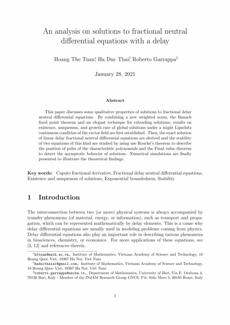
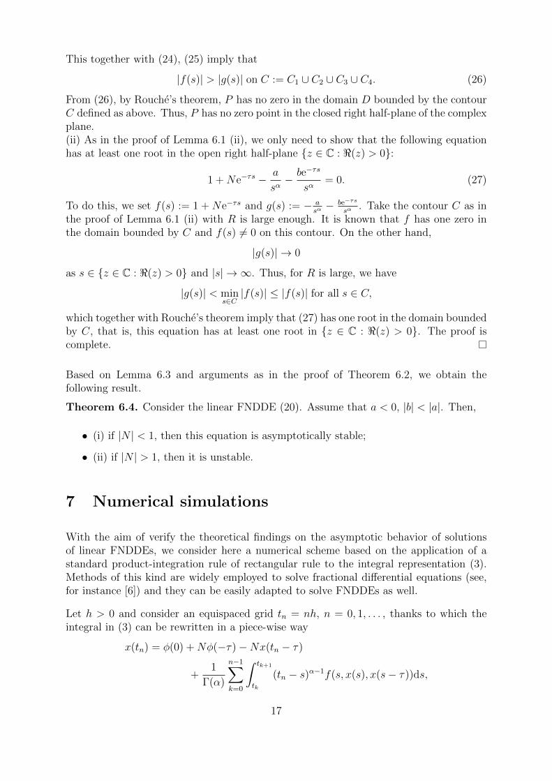
Figure 1: Trajectory of the solution Φ(·, φ) to system (28) when φ(t) = 0.2 on [−1, 0].

and hence the vector field f(s, x(s), x(s− τ)) is approximated in each interval [tk, tk+1] bythe constant values assumed in one of the endpoints of [tk, tk+1]. For stability reasons, andavoid to introduce in the simulations spurious instabilities, we prefer to device an implicitmethod and adopt the approximation f(s, x(s), x(s − τ)) ≈ f(tk+1, x(tk+1), x(tk+1 − τ)),s ∈ [tk, tk+1]. After integrating in an exact way each integral we obtain the approximationsxn ≈ x(tn)

xn = φ(0) +Nφ(−τ)−Nx(tn − τ) + hαn∑k=1

b(α)n−kf(tk, xk, xk−τ/h),

where convolution weights bn are defined as b(α)n = ((n + 1)α − nα)/Γ(α + 1). The ap-

proximation xk−τ/h of x(tk − τ) is obtained by interpolation of the two closest availableapproximations of the solution when tk − τ is not a grid point and when it does notbelong to [−τ, 0]. First-degree polynomial interpolation is clearly sufficient to preservethe first-order convergence of the PI rule. Finally, Newton-Raphson iterations are usedto determine xn from the above implicit scheme.

We now apply the above scheme to present some numerical examples illustrating the mainresults proposed in this paper.

Example 7.1. Consider the equation

CD0.70+

[x(t) + x(t− 1)

]= −5x(t), t > 0 (28)

x(·) ∈ C([−1, 0];R).

This equation is stable. In Figure 1, we simulate a trajectory of the solution Φ(·, φ) to(28) with the initial condition φ(t) = 0.2 on [−1, 0].

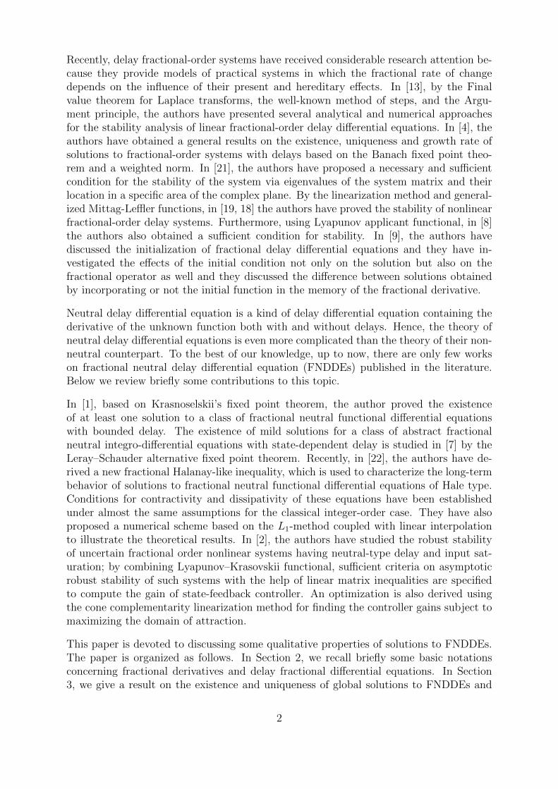
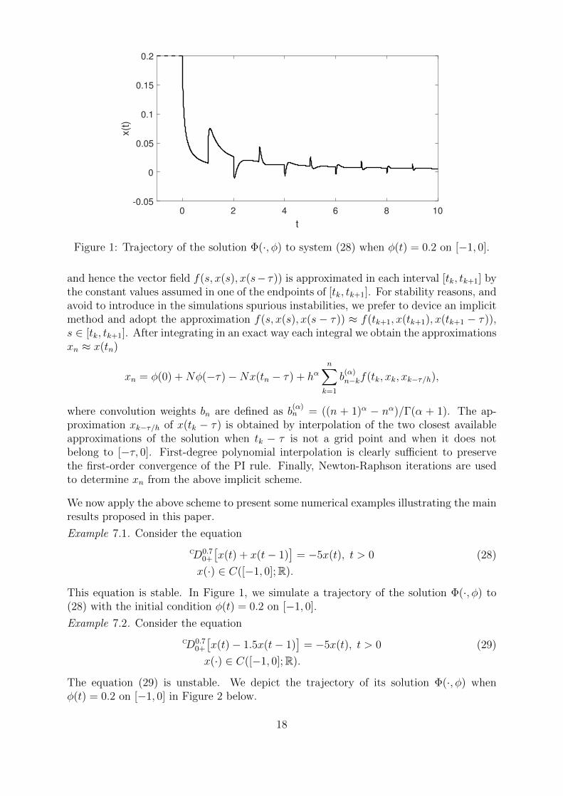
Example 7.2. Consider the equation

CD0.70+

[x(t)− 1.5x(t− 1)

]= −5x(t), t > 0 (29)

x(·) ∈ C([−1, 0];R).

The equation (29) is unstable. We depict the trajectory of its solution Φ(·, φ) whenφ(t) = 0.2 on [−1, 0] in Figure 2 below.

18

-2 0 2 4 6 8 10t

-0.4

-0.2

0

0.2

0.4

x(t)

Figure 2: Trajectory of the solution Φ(·, φ) to system (29) when φ(t) = 0.2 on [−1, 0].

19

0 2 4 6 8 10

t

0

0.05

0.1

0.15

0.2

x(t

)

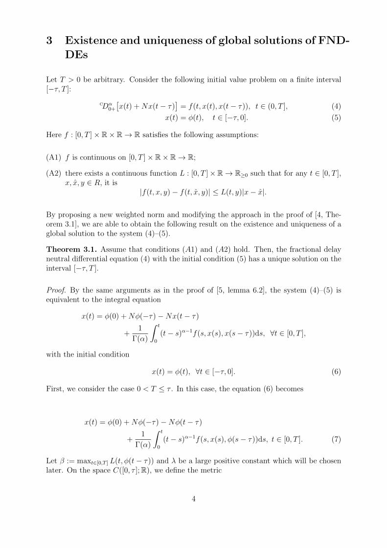
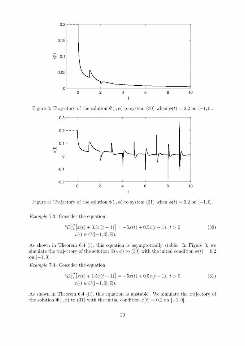
Figure 3: Trajectory of the solution Φ(·, φ) to system (30) when φ(t) = 0.2 on [−1, 0].

0 2 4 6 8 10

t

-0.2

-0.1

0

0.1

0.2

0.3

x(t

)

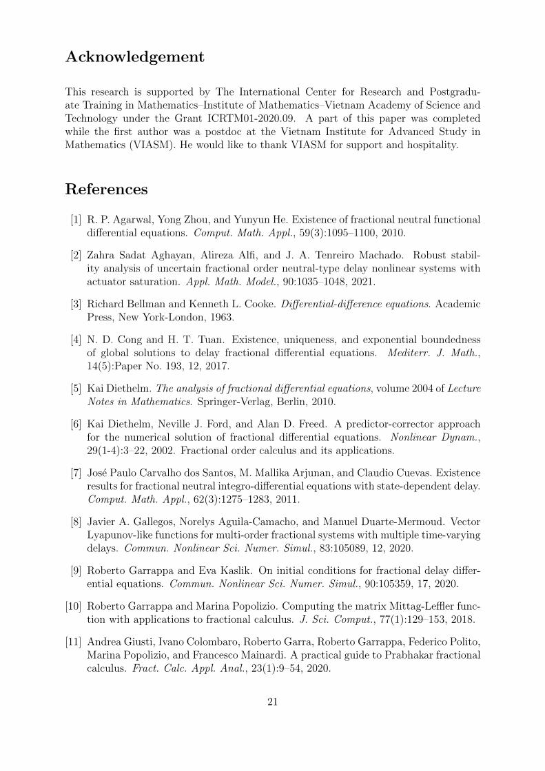
Figure 4: Trajectory of the solution Φ(·, φ) to system (31) when φ(t) = 0.2 on [−1, 0].

Example 7.3. Consider the equation

CD0.70+

[x(t) + 0.5x(t− 1)

]= −5x(t) + 0.5x(t− 1), t > 0 (30)

x(·) ∈ C([−1, 0];R).

As shown in Theorem 6.4 (i), this equation is asymptotically stable. In Figure 3, wesimulate the trajectory of the solution Φ(·, φ) to (30) with the initial condition φ(t) = 0.2on [−1, 0].

Example 7.4. Consider the equation

CD0.70+

[x(t) + 1.5x(t− 1)

]= −5x(t) + 0.5x(t− 1), t > 0 (31)

x(·) ∈ C([−1, 0];R).

As shown in Theorem 6.4 (ii), this equation is unstable. We simulate the trajectory ofthe solution Φ(·, φ) to (31) with the initial condition φ(t) = 0.2 on [−1, 0].

20

Acknowledgement

This research is supported by The International Center for Research and Postgradu-ate Training in Mathematics–Institute of Mathematics–Vietnam Academy of Science andTechnology under the Grant ICRTM01-2020.09. A part of this paper was completedwhile the first author was a postdoc at the Vietnam Institute for Advanced Study inMathematics (VIASM). He would like to thank VIASM for support and hospitality.

References

[1] R. P. Agarwal, Yong Zhou, and Yunyun He. Existence of fractional neutral functionaldifferential equations. Comput. Math. Appl., 59(3):1095–1100, 2010.

[2] Zahra Sadat Aghayan, Alireza Alfi, and J. A. Tenreiro Machado. Robust stabil-ity analysis of uncertain fractional order neutral-type delay nonlinear systems withactuator saturation. Appl. Math. Model., 90:1035–1048, 2021.

[3] Richard Bellman and Kenneth L. Cooke. Differential-difference equations. AcademicPress, New York-London, 1963.

[4] N. D. Cong and H. T. Tuan. Existence, uniqueness, and exponential boundednessof global solutions to delay fractional differential equations. Mediterr. J. Math.,14(5):Paper No. 193, 12, 2017.

[5] Kai Diethelm. The analysis of fractional differential equations, volume 2004 of LectureNotes in Mathematics. Springer-Verlag, Berlin, 2010.

[6] Kai Diethelm, Neville J. Ford, and Alan D. Freed. A predictor-corrector approachfor the numerical solution of fractional differential equations. Nonlinear Dynam.,29(1-4):3–22, 2002. Fractional order calculus and its applications.

[7] Jose Paulo Carvalho dos Santos, M. Mallika Arjunan, and Claudio Cuevas. Existenceresults for fractional neutral integro-differential equations with state-dependent delay.Comput. Math. Appl., 62(3):1275–1283, 2011.

[8] Javier A. Gallegos, Norelys Aguila-Camacho, and Manuel Duarte-Mermoud. VectorLyapunov-like functions for multi-order fractional systems with multiple time-varyingdelays. Commun. Nonlinear Sci. Numer. Simul., 83:105089, 12, 2020.

[9] Roberto Garrappa and Eva Kaslik. On initial conditions for fractional delay differ-ential equations. Commun. Nonlinear Sci. Numer. Simul., 90:105359, 17, 2020.

[10] Roberto Garrappa and Marina Popolizio. Computing the matrix Mittag-Leffler func-tion with applications to fractional calculus. J. Sci. Comput., 77(1):129–153, 2018.

[11] Andrea Giusti, Ivano Colombaro, Roberto Garra, Roberto Garrappa, Federico Polito,Marina Popolizio, and Francesco Mainardi. A practical guide to Prabhakar fractionalcalculus. Fract. Calc. Appl. Anal., 23(1):9–54, 2020.

21

[12] Jack K. Hale and Sjoerd M. Verduyn Lunel. Introduction to functional-differentialequations, volume 99 of Applied Mathematical Sciences. Springer-Verlag, New York,1993.

[13] Eva Kaslik and Seenith Sivasundaram. Analytical and numerical methods for thestability analysis of linear fractional delay differential equations. J. Comput. Appl.Math., 236(16):4027–4041, 2012.

[14] Igor Podlubny. Fractional differential equations, volume 198 of Mathematics in Sci-ence and Engineering. Academic Press, Inc., San Diego, CA, 1999.

[15] Tilak Raj Prabhakar. A singular integral equation with a generalized Mittag Lefflerfunction in the kernel. Yokohama Math. J., 19:7–15, 1971.

[16] Stefan G. Samko, Anatoly A. Kilbas, and Oleg I. Marichev. Fractional integrals andderivatives. Gordon and Breach Science Publishers, Yverdon, 1993.

[17] Joel L. Schiff. The Laplace transform. Undergraduate Texts in Mathematics.Springer-Verlag, New York, 1999. Theory and applications.

[18] H. T. Tuan and H. Trinh. A qualitative theory of time delay nonlinear fractional-ordersystems. SIAM J. Control Optim., 58(3):1491–1518, 2020.

[19] Hoang The Tuan and Hieu Trinh. A linearized stability theorem for nonlinear delayfractional differential equations. IEEE Trans. Automat. Control, 63(9):3180–3186,2018.

[20] Gennadi Vainikko. Which functions are fractionally differentiable? Z. Anal. Anwend.,35(4):465–487, 2016.

[21] Jan Cermak, Jan Hornıcek, and Tomas Kisela. Stability regions for fractional dif-ferential systems with a time delay. Commun. Nonlinear Sci. Numer. Simul., 31(1-3):108–123, 2016.

[22] Dongling Wang, Aiguo Xiao, and Suzhen Sun. Asymptotic behavior of solutions totime fractional neutral functional differential equations. J. Comput. Appl. Math.,382:113086, 13, 2021.

22