An Analysis of So-Called Export-led Growth; Jie Yang; IMF Working

An Analysis of So-Called Export-led Growth

Jie Yang

WP/08/220

© 2008 International Monetary Fund WP/08/220 IMF Working Paper Finance Department

An Analysis of So-Called Export-led Growth

Prepared by Jie Yang1

Authorized for distribution by Jianhai Lin

September 2008

Abstract

This Working Paper should not be reported as representing the views of the IMF. The views expressed in this Working Paper are those of the author(s) and do not necessarily represent those of the IMF or IMF policy. Working Papers describe research in progress by the author(s) and are published to elicit comments and to further debate.

The stylized fact that strong economic growth is usually accompanied with strong export growth leads many people to conclude that the export sector is the main driving force behind those episodes. The model in this paper, however, shows that the non-tradable sector may also generate high economic growth together with high export growth. Evidence shows that out of 71 “so-called” export-led growth episodes, only 37 of them are consistent with the “exports driving growth” hypothesis. Most of the remaining episodes (24 cases) experienced significant real exchange rate depreciation and are more likely to be characterized by “growth driving exports”. JEL Classification Numbers: F01, O41, O57 Keywords: Export-led growth, real exchange rate, productivity improvement Author’s E-Mail Address: [email protected]

1 The author would like to thank Arnold Harberger, Sebastian Edwards, and Kenneth Sokoloff for their insightful advice. This paper has greatly benefited from comments of Ratna Sahay, Jianhai Lin, and Aaron Tornell. I am also grateful to my colleagues at the IMF Finance Department Seminar, including Patrick Njoroge, Roberto Perrilli, Shaun Roache, and Marco Rossi, as well as conference participants at the 2008 Chinese Economist Society Annual Conference and seminar participants at the International Economics Seminar at UCLA.

2

Contents Page

I. Introduction………………………………………………………...…………………...3

II. Stylized Fact: High Economic and High Export Growth ………………………..…….5

III. The Model ………………………..…………………………………………………...8 A. The Comparative Static Version …………………………………………..………8 B. The Dynamic Version ……………………………………..……………………..13 C. Changing Assumptions on Elasticity …………………..……………….....……..17

IV. Empirical Evidence ………………………………………………..……..……….…18

A. Real Exchange Rate Movement in High Growth Periods ……………….........….18 B. Labor Productivity ………………..……………………………………..……..…18 C. Empirical Evidence: “Export Driving Growth” vs. “Growth Driving Exports” ....19

V. Conclusion ……………………………………..…………………………………….21 Reference …………………………………………………..………………………...….22 Figures Figure 1: Model Results of a Technological Advance in the Exportable Sector ….....…26 Figure 2: Model Results of a Technological Advance in the Nontradable Sector ..….....27 Figure 3: An Exogenous Positive Supply Shock in the Exportable Sector …………..…28 Figure 4: An Exogenous Positive Supply Shock in the Nontradable Sector ………..…..30 Tables Table 1: GDP Growth and Export Growth in High Growth Episodes ……..……….…..32 Table 2: Summary: GDP and Export Growth in High Growth Episodes …………...…..35 Table 3: Real Exchange Rate Movement in High Growth Episodes ………..…………..35 Table 4: Changes in the Equilibrium Home Goods price and in Wages ……..................36 Table 5: Changes in the Equilibrium Home Goods Price and in Wages …………..……37 Table 6: Summary of Model Results ………………………..…………………………..38 Table 7: Industrial Classification of Tradable and Nontradable Sector ……………..… .38 Table 8: Productivity Growth in Tradable Sector relative to Nontradable Sector and Real

Exchange Rate Movement in High Growth Episodes …………..…………….39 Table 9: "Exports Driving growth" vs. "Growth Driving Exports" ………………..……42

3

I. Introduction

The past half century has witnessed an unprecedented rate of world economic development. One stylized fact found by many empirical studies is that most high growth episodes are usually characterized by high export growth, which leads many people to the conclusion that the export sector has played a leading role in the growth process. For example, Balassa (1978) and Ram (1985) found that exports played an important role in promoting economic growth by conducting cross-country comparison or regressing GDP growth on different export variables. Especially after the very success of the Asian Tigers (Hong Kong Special Administrative Region, The Republic of Korea, Taiwan Province of China, and Singapore) in pursuing an export-driven model of economic development, many countries followed their pattern and directed, as a result, a great deal of attention to the exportable sector when designing economic policies. Successful growth episodes exhibiting high export growth are therefore usually labeled “export-led growth”. If “export-led growth” was the true explanation for those high GDP growth episodes accompanied by high export growth, we should have been able to observe real exchange rate appreciation in all such episodes (due to the influx of foreign exchange) as a result of booming exports. The data show, however, that this real exchange rate appreciation has only occurred in around half of those so-called “export-led growth” episodes. The real exchange rate actually depreciated in many episodes characterized by high economic growth together with high export growth, which leads to doubts as to how safely such episodes can be claimed as “export-led growth”. This further leads to the question whether some forces other than booming exports can generate high growth of both exports and GDP. In this paper, a model is developed to study the relationship among productivity improvements in the tradable or the non-tradable sector, economic growth, and export growth. “export-led growth” is considered to only mean a case where the dominant underlying cause of economic growth is an exogenous increase in export activities. When such a model is followed, the result of “export-led growth” stemming from an exogenous increase in export productivity is a simultaneous occurrence of high economic growth, high export growth, and real exchange rate appreciation. And in such cases, it is “exports driving growth”. This paper shows next that it is quite possible for both exports and GDP to grow without exports being the exogenous source of GDP growth. This can occur even when the only exogenous factor is an improvement in productivity in the nontradable sector. Such an improvement has its first effect on GDP itself, which in turn causes demand to increase in all major sectors of the economy. If the income elasticity of demand for importables is large, increased demand for imports will cause the real exchange rate to depreciate, which stimulates exports to grow and leads to the same set of phenomena that many people characterize as “export-led growth”. When money is introduced into the dynamic version of this model, exports will have to increase even more to meet the need of accumulating more foreign exchange reserves as the economy grows. In cases like this, it is actually “growth driving exports” that links high GDP

4

growth with high export growth. In conclusion, the model shows that productivity improvement in either the tradable sector or the nontradable sector may generate high GDP growth and high export growth. Therefore, one should not make the mistake of thinking that high growth together with high export growth is an absolute signal of “export-led growth”. A better way to understand the role of productivity in the growth process is to give it a broader interpretation in terms of “real cost reduction” (Harberger 1998). After all, “technology” is the residual part of growth that is left unexplained by the contribution of capital and labor in the growth accounting equation. While labels like “TFP improvements” or “technical changes” direct most attention to research and development or externalities of different kinds (e.g. economies of scale, spillovers, and systematic complementarities), “real cost reduction” broaden people's eyes to see thousands of ways used by firms to cut the real cost of their production, such as computerizing the payroll system or hiring a more strict manager who pushes his employees to work harder. All these activities are accounted in the part of “technology” in growth accounting, in the sense that they allow firms to extract more outputs from the same set of inputs. The concept of “real cost reduction” also helps understand the thousands of ways in which productivity improvements can occur in the nontradable sector. Thinking of the success of chain stores such as Wal-Mart and K-Mark, the fast-growing telecommunication industry, the cheap air tickets, and the IT revolution, these are just a few examples of the dramatic productivity improvements in the nontradable sector. Therefore, productivity improvement labeled as “real cost reduction” happens widely across different industries in the economy, including both the tradable and the nontradable sectors. Thus, the link between high growth and high export growth can be due to either a productivity improvement in the tradable or the nontradable sector, i.e. “exports driving growth” scenario or “growth driving exports” scenario, as suggested by the model. How can these two scenarios be distinguished? Many recent studies try to test the causality between exports and economic growth by applying "Granger Causality" test in their econometric regression. The conclusions from those papers are somehow mixed. For example, Kwan and Kwok (1995) found that China’s growth is the “export-led” type while Boltho (1996) found that Japan’s economic growth was mainly due to the domestic forces rather than foreign demand. The model in this paper suggests that calibrating TFP growth in the tradable and the non-tradable sector may reveal the true underlying forces for high economic growth together with high export growth. However, TFP is not directly measurable due to data unavailability at industry level in many developing countries. The model, then, suggests that the real exchange rate serves a good candidate to distinguish “exports driving growth” and “growth driving exports”. In the first case, the real exchange rate appreciates due to the increased supply of exports; and in the second case, it depreciates due to increased demand of imports.

5

Using data on 44 countries over the period from 1958-2004, this paper examines how many successful growth episodes represent “exports driving growth”, and how many represent “growth driving exports” ones. Since TFP is not directly measurable due to lack of data on capital at industry level, I examine the relative labor productivity growth in the tradable sector compared to the nontradable sector and the behavior of the real exchange rate, which serve as good indicators of true underlying forces as suggested by the model. In all 71 high growth episodes that were accompanied by an even higher growth of exports across different countries, which look like “export-led growth” at first glance, only 37 of them experienced real exchange rate appreciation and thus are consistent with the “export-led growth” hypothesis. For another 24 episodes, the results suggest that the dominant exogenous force was an increase in the supply of nontradables, relative to that of tradables. In these cases, despite a high export growth and a high GDP growth as well, the real exchange rate depreciates. Another six episodes experienced insignificant changes both in the real exchange rate and the tradable/nontradable labor productivity ratio. This suggests that technological advances were of similar relative importance in the exportable sector and in the nontradable sector, a result that is still compatible with high economic growth and high export growth. Therefore, the “export-led growth” explanation is not the dominant underlying force for this set of successful growth episodes characterized by high export growth. The nontradable sector plays an equally important role as the export sector in generating high economic growth and high export growth.

This conclusion that many alleged “export-led growth” episodes were actually led by the nontradable productivity improvements may have policy implications for developing countries. Across the whole set of developing economies, we see a lot of export-promotion policy implemented by the government with the hope of stimulating economic growth via the export sector. However, by examining real exchange rate movements in high export and GDP growth episodes, this paper shows that it is then the nontradable sector appears to drive the GDP-cum-export growth process in many high export and economic growth episodes. This suggests that countries should be cautious about giving special policy privileges to the export sector. The government should better pursue non-discriminatory growth policies that encourage technological improvements in all industries, both tradable and nontradable, instead of focusing on preferential stimulation of export activities.

The remainder of the paper is organized as follows. Section II explores the behavior of exports and real exchange rate during high growth episodes in 43 countries. Section III introduces the model, which studies the effect of different types of productivity shocks on exports, the real exchange rate and economic growth, both in a comparative static version and in a dynamic version. Section IV presents data on relations between productivity and the real exchange rate in those high growth episodes. Section V offers some concluding remarks and policy implications.

II. Stylized Fact: High Economic Growth and High Export Growth

6

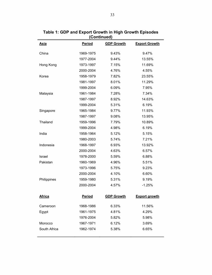
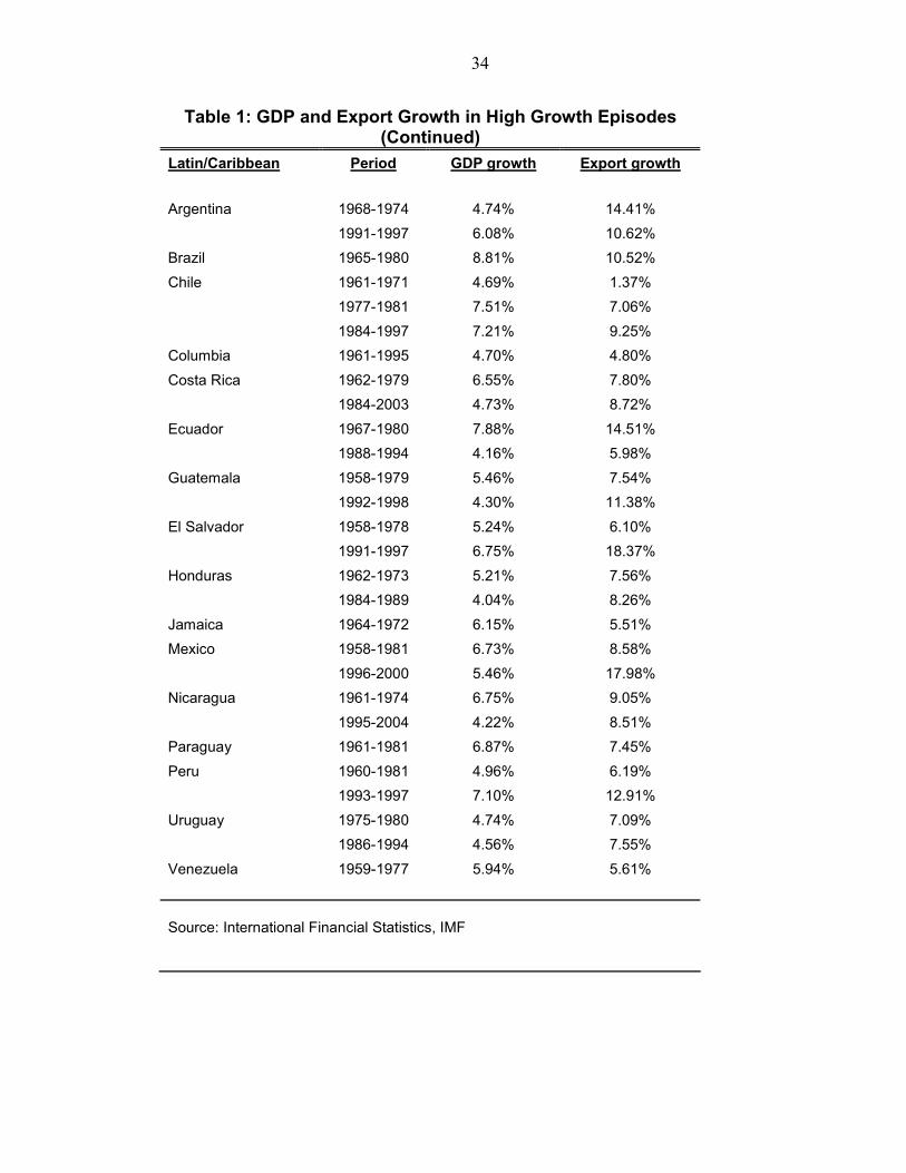
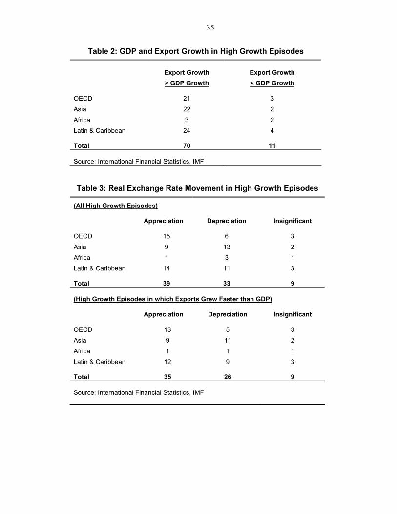
Although it is not easy to find simple factors that are shared by the episodes of many different countries’ successful economic development, one point widely agreed among economists is the importance of trade liberalization, which allows the country to make the most of its own comparative advantage in the international market. One measure of the degree of such openness is the course of its exports. Table 1 presents data on GDP growth and export growth in a large number of high-growth episodes, covering the period 1958-2004, depending on the data availability of different country. A high-growth episode is defined as one where GDP growth averaged over four percent a year for a period of at least five years (Harberger 2005), and, throughout the whole high growth episode, there cannot be any negative growth rate for any year. In all, 81 high growth episodes are identified, 24 episodes in 11 OECD countries, 24 episodes in 11 Asian countries, five episodes in five African countries, and 28 episodes in 16 Latin American or Caribbean countries. Most of these high growth episodes display average GDP growth rates between four and seven percent a year. A few countries, such as the Asian Tiger, have averages between seven to ten percent. In nearly all these high growth episodes, high GDP growth is found to be usually accompanied by a surge in exports. An even more striking fact is that exports grew faster than GDP during those high growth episodes. As summarized in Table 2, in 70 out of 81 high growth episodes in total, exports grow at a much faster rate than GDP. This strong link between export growth and GDP growth has led many people to believe that the main engine of high economic growth in those countries is an export boom, most likely driven either by a technological advancement in the export production, or by an increase in the world price of the main export commodities. To explain the faster rate of export growth than GDP growth, one can think of a technological improvement in the exportable sector. The production of exportable goods then enjoys a competitive advantage in the international market. Given the country is not big enough to affect the world price, the profit margin for producing the exportable goods simply rises. More exportable goods will be produced by existing firms, and more producers will be attracted to enter the exportable industry by the profit opportunities. Labor, capital, and other resources will be pulled into the exportable sector from other main sectors, which makes the exportable production typically grow more than GDP itself2. The increase in the main export products influences the economy in a similar way.3 In such circumstances, the economic 2 There can be anomalous cases in which a technological improvement in the export sector generates an export growth that is not as high as the GDP growth. For example, in an extreme case in which some natural resources used as input in export production are only available in fixed quantity, then a technological advance in the export sector will take place in terms of using less labor and capital combined with the given amount of natural resources. In such setting, the export sector releases labor and capital to other sectors in the economy and GDP may grow faster than exports.

3 One can use a scenario of exogenous productivity growth in the export sector to also cover the case of a rise in the world price of a country's principal export product. In both cases, the same resources that were previously used to pay for a given quantity of imports can, after the exogenous shock, pay for a significantly greater amount.

7

growth is truly initiated by the exportable sector. This is the main story of the “export-led” growth in which exports are strongly correlated with economic growth. If export-led growth was the leading phenomena among those high GDP and high export growth episodes, economic theory predicts that such export boom leads to an appreciation of the real exchange rate because more foreign currency is received as proceeds from exports. If people spent all of the incremental foreign currency on tradables, the increments of supply and the demand of foreign currency in real terms would be the same, and the real exchange rate would not change. But much more likely, part of the incremental foreign currency will be spent on nontradables, in which case the real exchange rate appreciates as people exchange foreign currency for domestic currency in order to consume home goods. Therefore, if a technological advance in the exportable sector or an increase in the main export products is the dominant force driving the high GDP growth, we should have been able to observe real exchange rate appreciation in all those high growth episodes.4 Table 3 presents the real exchange rate movement in the 81 high growth episodes identified earlier. In fact, only 39 high growth episodes experienced an appreciation of the real exchange rate, while 33 others experienced a depreciation, and nine experienced an insignificant change in the real exchange rate. Even if only look at those episodes in which exports grew faster than GDP and are more likely to be the export-led growth story, we still find that only half (35 cases out of 70) experienced real exchange rate appreciation, while most of the other half experienced a real exchange rate depreciation. The evidence that the real exchange rate did not appreciate in all these high GDP and high export growth episodes leads to doubts how safely such episodes may be identified as “export-led growth”, i.e., “exports driving growth”. The question this paper then ask is whether some forces other than booming exports can generate high GDP and high export growth together with real exchange rate depreciation. This paper will show that one likely answer to the above question is an exogenous technological improvement in the nontradable sector. Such productivity improvement has its primary effect directly on the economic growth. Then as the economy grows, people demand more of all kinds of goods, including exportables, importables, and nontradables. If income elasticity of demand for importable is sufficiently large, imports will grow and the only way to pay for increased imports is to have exports grow.5 Therefore, a technological improvement in the nontradable sector may also drive both GDP and

4 Obviously, other factors, such as capital outflow could have a stronger influence on the movement of the real exchange rate, leading to real exchange rate depreciation. We would say that in such cases, TFP improvement in the export sector is not the dominant disturbance.

5 The imports can be paid by things other than exports, such as capital inflow, in the short run. But in the long run, trade account has to be balanced and the country's imports have to equal its exports.

8

exports to grow. To explore the true underlying driving force behind those episodes in which both GDP and exports grew dramatically, a model is developed in the following section to examine respectively the influence of a technological change in the tradable and the nontradable sector on export growth, economic growth, and the real exchange rate.

III. The Model

This model aims to study how technological improvements that occur in different sectors of the economy stimulate high output growth and high export growth. The model is presented both in a comparative static form and in a dynamic form.

A. The Comparative Static Version

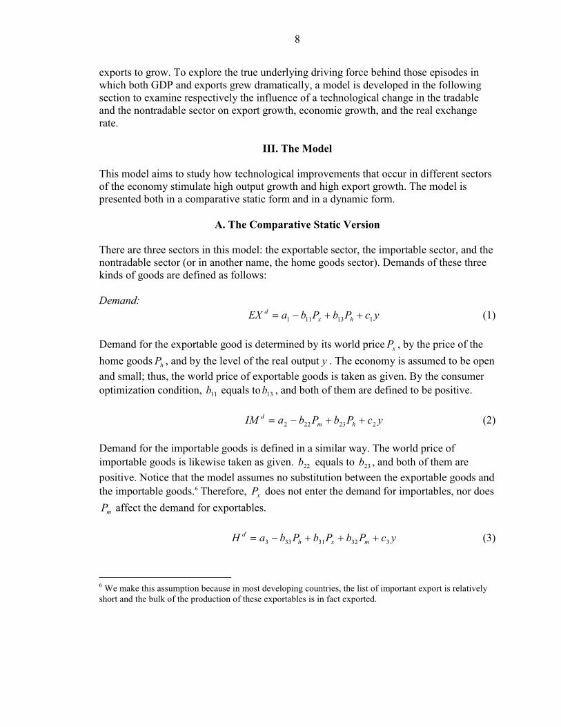
There are three sectors in this model: the exportable sector, the importable sector, and the nontradable sector (or in another name, the home goods sector). Demands of these three kinds of goods are defined as follows:

Demand:

ycPbPbaEX hxd

113111 ++−= (1)

Demand for the exportable good is determined by its world price xP , by the price of the home goods hP , and by the level of the real output y . The economy is assumed to be open and small; thus, the world price of exportable goods is taken as given. By the consumer optimization condition, 11b equals to 13b , and both of them are defined to be positive.

ycPbPbaIM hmd

223222 ++−= (2)

Demand for the importable goods is defined in a similar way. The world price of importable goods is likewise taken as given. 22b equals to 23b , and both of them are positive. Notice that the model assumes no substitution between the exportable goods and the importable goods.6 Therefore, xP does not enter the demand for importables, nor does

mP affect the demand for exportables.

ycPbPbPbaH mxhd

33231333 +++−= (3)

6 We make this assumption because in most developing countries, the list of important export is relatively short and the bulk of the production of these exportables is in fact exported.

9

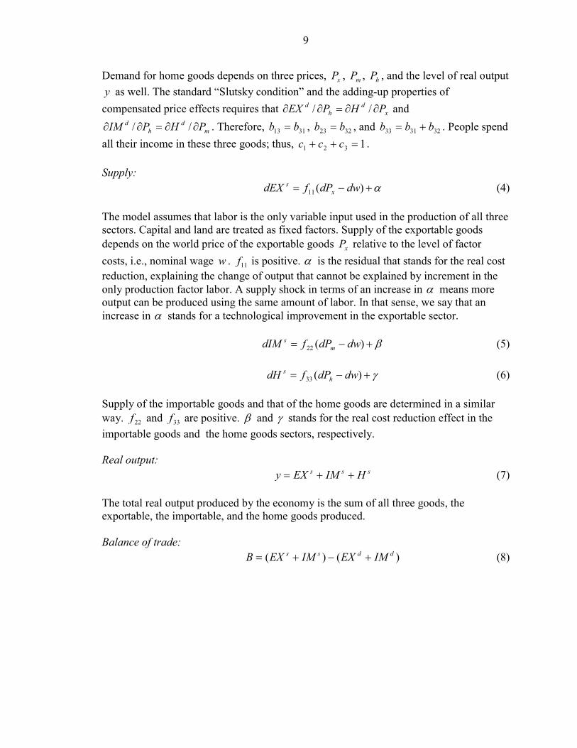
Demand for home goods depends on three prices, xP , mP , hP , and the level of real output y as well. The standard “Slutsky condition” and the adding-up properties of compensated price effects requires that x

dh

d PHPEX ∂∂=∂∂ // and

md

hd PHPIM ∂∂=∂∂ // . Therefore, 3113 bb = , 3223 bb = , and 323133 bbb += . People spend

all their income in these three goods; thus, 1321 =++ ccc . Supply: α+−= )(11 dwdPfdEX x

s (4) The model assumes that labor is the only variable input used in the production of all three sectors. Capital and land are treated as fixed factors. Supply of the exportable goods depends on the world price of the exportable goods xP relative to the level of factor costs, i.e., nominal wage w . 11f is positive. α is the residual that stands for the real cost reduction, explaining the change of output that cannot be explained by increment in the only production factor labor. A supply shock in terms of an increase in α means more output can be produced using the same amount of labor. In that sense, we say that an increase in α stands for a technological improvement in the exportable sector. β+−= )(22 dwdPfdIM m

s (5) γ+−= )(33 dwdPfdH h

s (6) Supply of the importable goods and that of the home goods are determined in a similar way. 22f and 33f are positive. β and γ stands for the real cost reduction effect in the importable goods and the home goods sectors, respectively. Real output: sss HIMEXy ++= (7) The total real output produced by the economy is the sum of all three goods, the exportable, the importable, and the home goods produced. Balance of trade: )()( ddss IMEXIMEXB +−+= (8)

10

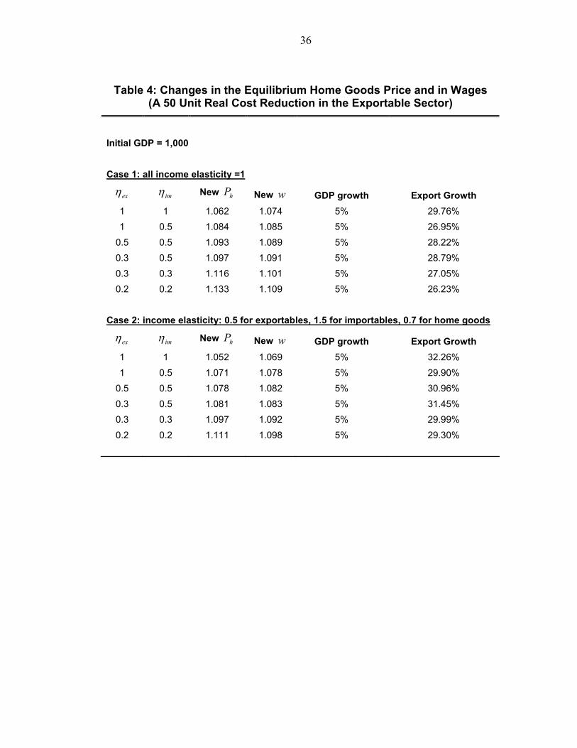
The balance of trade is defined as the excess supply of tradable goods, exportable plus importable goods, to the demand of tradable goods.7 It assumes that the economy starts with an initial equilibrium in which all prices ( xP , mP , and hP ) and the wage ( w ) are calibrated to one. xP (= mP ) is used as numeraire in this model, i.e., world prices of both exportables and importables are taken as given. Since there is no trade of home goods with the rest of the world, demand for home goods always equals their supply in any equilibrium. It further assumes that the home goods market starts with an equilibrium in which dH and sH are both 500. Demand for the exportable goods dEX in the initial equilibrium is assumed to be 100 and that for the importable goods dIM is 400. The supply of the exportable goods sEX and that of the importable goods sIM are assumed to be 300 and 200 respectively. Exports equal the excess supply of exportables, which is 200. Imports equal to the excess demand for importables, which is also 200. Therefore, the trade account is balanced in this initial equilibrium. The initial equilibrium real output is 1000. A Technological Advance in the Exportable Sector The model firstly studies the effect of an exogenous positive supply shock in terms of a 50 unit real cost reduction8 that occurs in the exportable sector. The direct effect of this shock is that the exportable sector can produce 50 units more of exportables using the same amount resources as before. The economy’s total output, therefore, increases by 50, which is an output growth rate of five percent.9 The new equilibrium is solved by the following two conditions: 50=++ sss dHdIMdEX (9) sd dHdH = (10) These two conditions stand for the resource constraint and the home goods market clearing condition respectively. Different values of the price elasticity of demand for the exportable goods exη , that for the importable goods imη , and the income elasticity of demand for importables 2c are assumed to study their effect on the final equilibrium.

7 Balance of trade can also be defined as exports minus imports. These two definitions are actually equivalent.

8 See Harberger 1998 for more details on the concept of "real cost reduction"

9 This is true regardless of: a) the exportable sector ends up producing more than 350 units, in which case it will absorb additional resources from the other sectors of the economy, or b) the exportable sector ends up producing less than 350 units, in which case it will release resources to the other sectors.

11

Values of supply elasticity are all assumed to be unity. The value of the price elasticity of demand for the home goods hη is implied (via the Slutsky condition) by the assumed value of exη and imη , plus the initial conditions. Table 4 reports the price of the home goods and the wage as well as the export growth and the GDP growth resulting from this technological improvement in the exportable sector. Not surprisingly, in all cases, exports boom due to both the direct and the indirect effect of the technological advance in terms of 50 unit real cost reduction in the exportable sector. The direct effect is that the exportable sector can simply produce 50 units more exportable goods using the same amount of resources as before. The indirect effect is that the exportable sector is now at a better comparative advantage in the world market, which induces more resource flow into the exportable sector from the other sectors in the economy. Meanwhile, as the exportable sector pulls labor from other sectors in the economy, the real wage10 increases in all cases to reflect the increased demand for labor in the exportable sector. As labor moves to the exportable sector and the nominal wage increases, supply of importable goods decreases for sure. In the home good sector, supply may increase or decrease, depending on the relative change in the nominal wage to that in the home good price. In all cases, however, the net flow of resources from the importable and the home good sector combined together to the exportable sector is positive. On the demand side, demand for all kinds of goods increases as the economy grows and income increases. Demand for exportable goods increases, but is small relative to the increase in supply, explaining why exports grow at a rate of about 30 percent in nearly all cases, which is much faster than the five percent growth rate of GDP. Demand for importables increases with people’s income level, combining with decrease in its supply, makes import grow as well. As a result, trade is balanced with a higher level of both exports and imports in the new equilibrium. Notice that export growth depends on the assumptions of elasticity as well. A bigger price elasticity of demand for the tradable goods relative to the home goods, a smaller price elasticity of demand for the exportable goods relative to the importable goods, or a bigger income elasticity of demand for the importable goods; all these make exports grow more. In the new equilibrium in all cases in Table 4, the home goods price increases by a range from five percent to 13 percent, depending on the value of elasticity assumed. In other words, the real exchange rate, measured in terms of the relative price of tradables to nontradables, appreciates. The intuition is that as exports grow, proceeds from the export activities generate an influx of foreign currency, which makes foreign currency cheaper relative to domestic currency. Therefore, the real exchange rate, which measures the relative real price of foreign currency in terms of domestic currency, appreciates. In 10 Real wage equals nominal wage divided by the weighted average price of tradable goods and home goods.

12

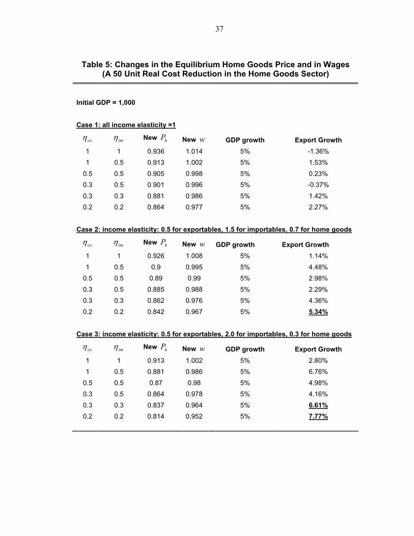
summary, when a country experiences an export boom, exports activities will take a leading role in stimulating economic growth. Such “exports driving growth” scenario generates not only high economic growth and even higher export growth, but also a real exchange rate appreciation. A Technological Advance in the Home Goods Sector Now I assume that a similar positive supply shock in terms of a 50 units of real cost reduction takes place in the home goods sector. Table 5 reports the new equilibrium resulting from this technological advance.

With such a technological advance, home goods are now produced at a more efficient scale. Nominal wage increases in some cases and decreases in other cases, which means the home good sector may or may not release resources to the other sectors in the economy. Real wage, however, increases in all cases, reflecting a competition for labor. Price of home goods decreases, implying that the real exchange rate depreciates in all cases.

What may seem unexpected is the fact that exports still grow in most cases; and grow at a even faster rate than GDP in a couple of cases. What is the driving force behind such export growth when the exogenous technological advance takes place only in the home goods sector? The key underlying force is people’s increased demand for importables as income grows. A technological advance in the home good sector has its first direct effect on the production of home goods and the economic growth. As people’s income level increases, demand increases in all major sectors of the economy. Given the assumption that the trade account has to be balanced in this comparative static model, the only way that the economy can finance its increased imports is to have exports grow as well. Such export growth is stimulated by real exchange rate depreciation resulting from people’s increased demand for foreign currency to buy more imports. Especially when the income elasticity of demand for importables is sufficiently large, exports may have to grow even faster than GDP in order to pay for the large increase in imports. In real life, a reasonable value of the price elasticity of demand for tradable goods falls between 0.2 and 0.3, implying a more likely occurrence of exports growing faster than GDP as shown in Table 5. Therefore, a real cost reduction taking place in the home goods sector may also generate high GDP together with an even higher export growth, just as occurs with a real cost reduction in the exportable sector. We call such a scenario “growth driving exports”, in which the real exchange rate depreciates, instead of appreciates, as it does in the “exports driving growth” scenario.

Therefore, one should be careful in reaching with judgments on what is the real underlying driving force when the phenomenon of both high GDP growth and high export growth is observed. The question now becomes what economic variable can best

13

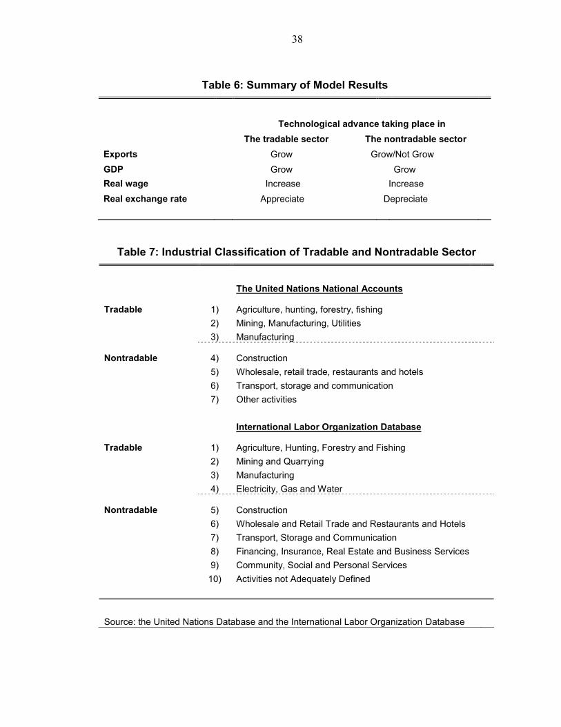
be used as an appropriate indicator to distinguish between “exports driving growth” and “growth driving exports”.11 Table 6 summarizes model results of these two scenarios and shows that the real exchange rate is a good candidate for such an indicator. In both scenarios, most likely, GDP and exports both grow. Thus, a co-occurrence of high GDP and high export growth does not help distinguish between “exports driving growth” and “growth driving exports”. Measuring TFP improvement in the tradable and the nontradable sector is another option and is actually the most direct indicator. However, in many developing countries, data are usually not sufficient to calibrate TFP at the sector level. Real wage increases in both scenarios. Therefore, the only candidate left is the real exchange rate, which appreciates in “exports driving growth” scenario and depreciates in “growth driving exports”.

B. The Dynamic Version

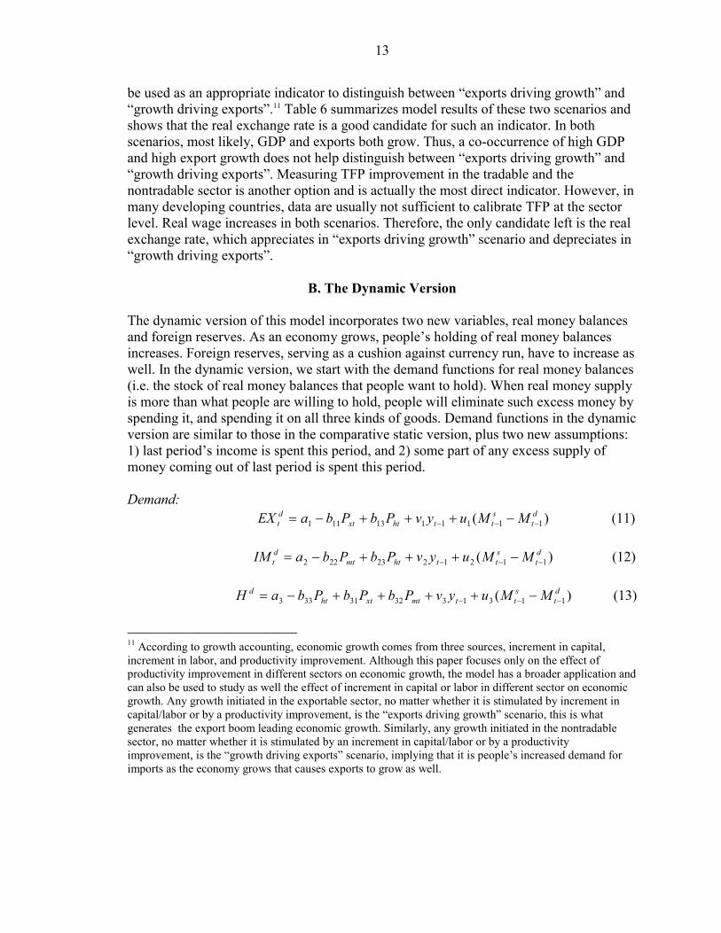
The dynamic version of this model incorporates two new variables, real money balances and foreign reserves. As an economy grows, people’s holding of real money balances increases. Foreign reserves, serving as a cushion against currency run, have to increase as well. In the dynamic version, we start with the demand functions for real money balances (i.e. the stock of real money balances that people want to hold). When real money supply is more than what people are willing to hold, people will eliminate such excess money by spending it, and spending it on all three kinds of goods. Demand functions in the dynamic version are similar to those in the comparative static version, plus two new assumptions: 1) last period’s income is spent this period, and 2) some part of any excess supply of money coming out of last period is spent this period.

Demand: )( 1111113111

dt

stthtxt

dt MMuyvPbPbaEX −−− −+++−= (11)

)( 1121223222

dt

stthtmt

dt MMuyvPbPbaIM −−− −+++−= (12)

)( 113133231333

dt

sttmtxtht

d MMuyvPbPbPbaH −−− −++++−= (13) 11 According to growth accounting, economic growth comes from three sources, increment in capital, increment in labor, and productivity improvement. Although this paper focuses only on the effect of productivity improvement in different sectors on economic growth, the model has a broader application and can also be used to study as well the effect of increment in capital or labor in different sector on economic growth. Any growth initiated in the exportable sector, no matter whether it is stimulated by increment in capital/labor or by a productivity improvement, is the “exports driving growth” scenario, this is what generates the export boom leading economic growth. Similarly, any growth initiated in the nontradable sector, no matter whether it is stimulated by an increment in capital/labor or by a productivity improvement, is the “growth driving exports” scenario, implying that it is people’s increased demand for imports as the economy grows that causes exports to grow as well.

14

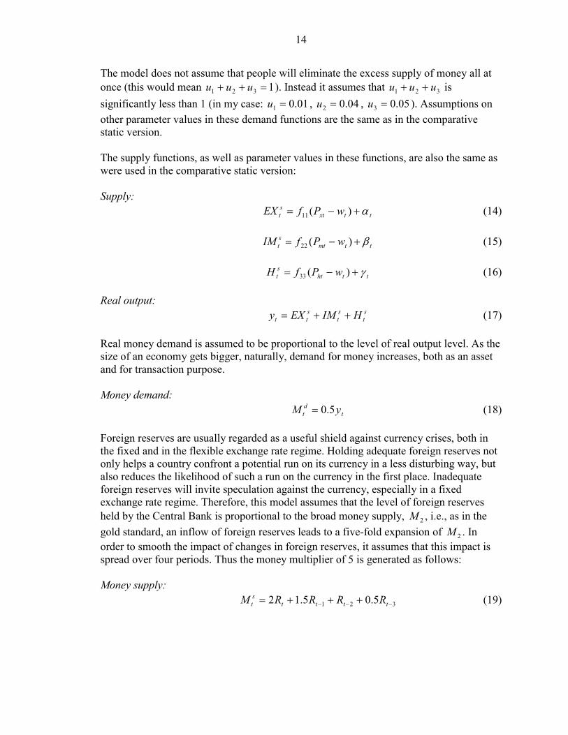
The model does not assume that people will eliminate the excess supply of money all at once (this would mean 1321 =++ uuu ). Instead it assumes that 321 uuu ++ is significantly less than 1 (in my case: 01.01 =u , 04.02 =u , 05.03 =u ). Assumptions on other parameter values in these demand functions are the same as in the comparative static version. The supply functions, as well as parameter values in these functions, are also the same as were used in the comparative static version: Supply: ttxt

st wPfEX α+−= )(11 (14)

ttmt

st wPfIM β+−= )(22 (15)

ttht

st wPfH γ+−= )(33 (16)

Real output: s

tst

stt HIMEXy ++= (17)

Real money demand is assumed to be proportional to the level of real output level. As the size of an economy gets bigger, naturally, demand for money increases, both as an asset and for transaction purpose. Money demand: t

dt yM 5.0= (18)

Foreign reserves are usually regarded as a useful shield against currency crises, both in the fixed and in the flexible exchange rate regime. Holding adequate foreign reserves not only helps a country confront a potential run on its currency in a less disturbing way, but also reduces the likelihood of such a run on the currency in the first place. Inadequate foreign reserves will invite speculation against the currency, especially in a fixed exchange rate regime. Therefore, this model assumes that the level of foreign reserves held by the Central Bank is proportional to the broad money supply, 2M , i.e., as in the gold standard, an inflow of foreign reserves leads to a five-fold expansion of 2M . In order to smooth the impact of changes in foreign reserves, it assumes that this impact is spread over four periods. Thus the money multiplier of 5 is generated as follows: Money supply: 321 5.05.12 −−− +++= tttt

st RRRRM (19)

15

In the comparative static version, exports are the only way to finance the economy’s imports; thus, they have to equal imports all the time. In the dynamic version, however, this constraint is removed. During transitional periods towards the new equilibrium, the excess of exports over imports is accumulated as foreign reserves, while any excess of imports over exports is paid by drawing down foreign reserves, until the economy reaches the new equilibrium and the trade account is once again balanced. Balance of trade: 1)()( −−==+−+= ttt

dt

dt

st

stt RRdRIMEXIMEXB (20)

The new equilibrium is characterized by two equilibrium conditions: the home goods market equilibrium condition (as in the comparative static version) and the new money market equilibrium condition. sd HH = (21) d

tst MM = (22)

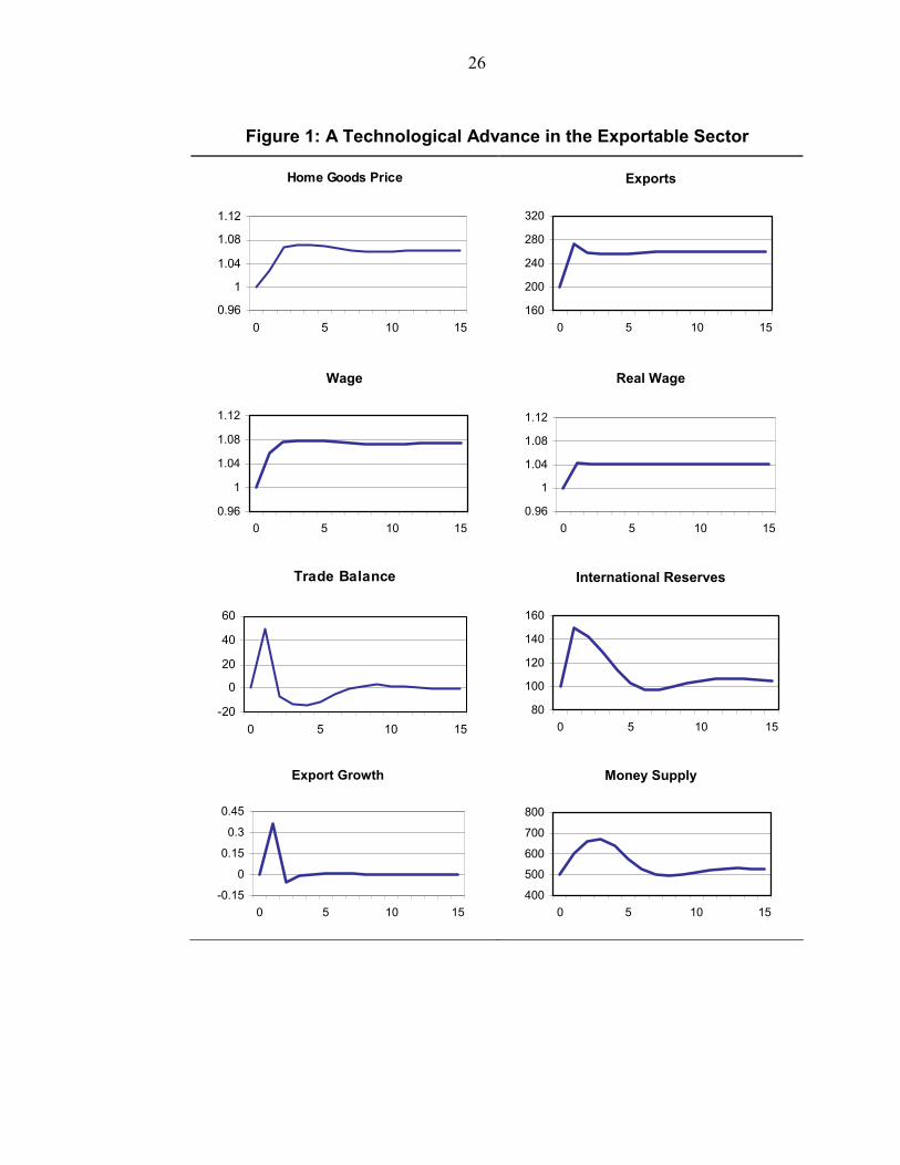
A Technological Advance in the Exportable Sector As in the comparative static version, the model first studies the effect of an exogenous positive supply shock in terms of a 50 unit real cost reduction taking place in the exportable sector. Values of the price elasticity of demand for exportable goods exη and that for importable goods imη are both assumed to be unity, so are values of supply elasticity in all three sectors. The value of the price elasticity of demand for the home goods hη is implied (via the Slutsky condition) by the assumed values of exη and imη , plus the initial conditions. Marginal propensities to spend on exportables, importables, and nontradables are assumed to be 0.1, 0.4 and 0.5 respectively.12 This set of assumptions is defined as the benchmark case and the paper will then compare it with other cases in which different elasticity assumptions are applied. Figure 1 reports the behavior of several economic variables during the transitional period after the shock in the benchmark case. The economy, as shown in Figure 1, converges to the new equilibrium quite fast --- in about 10 periods after the shock takes place. The resulting behavior of most economic variables in this dynamic version is very similar to what is observed in the comparative static version. The home good price increases, implying that the real exchange rate appreciates. Both the nominal wage and the real wage increase, reflecting a rising

12 Since the initial equilibrium has dEX =100, dIM =400, and dH =500, this implies that all three income elasticities of demand are equal to 1.

16

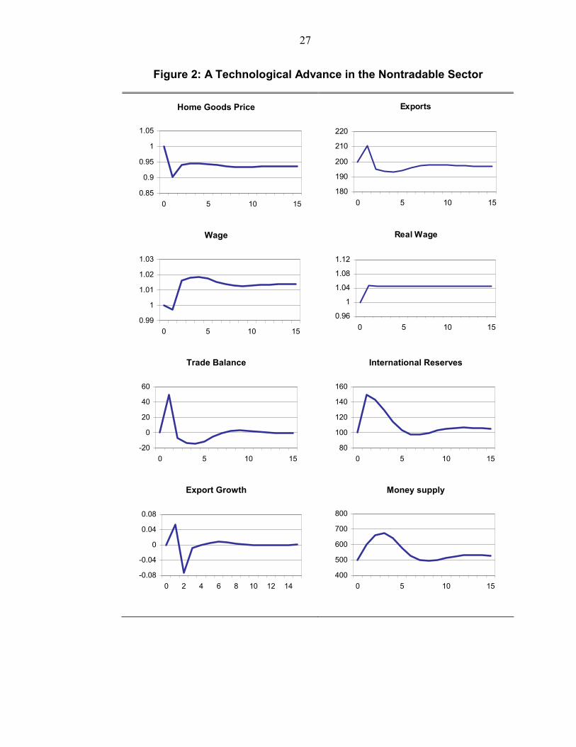
competition for labor as a result of the technological advance in the exportable sector. Exports grow and so does GDP. The cumulative increase in exports during the transitional periods, however, is more than that in imports. This is because in such a dynamic version in which money and foreign reserves are incorporated, exports are not only used to pay for imports, but also used to accumulate more foreign reserves to back up a bigger money supply in the new equilibrium. Therefore, export growth is higher during the transitional periods in this dynamic version than in the comparative static version. The balance of trade starts with a surplus account in the beginning due to the export boom, but finally adjusts to be zero as in the new equilibrium exports have to be balanced with imports again. The international reserves experience a rapid accumulation at the beginning, as a result of the influx of foreign currency from growing export activities, and then end up at a higher level than in the initial equilibrium, in order to back up a bigger money supply in the new equilibrium. In summary, a technological advance taking place in the exportable sector in this dynamic version generates results that are similar to those in the comparative static version, despite the fact that exports grow more than in the comparative static version due to the need for more foreign reserves in the new equilibrium. Such case is well qualified to be labeled as “exports driving growth”. A Technological Advance in the Home Goods Sector Now I study the effect of an exogenous positive supply shock in terms of a 50 unit real cost reduction taking place in the home goods sector. Figure 2 reports the movement of some key economic variables from the initial equilibrium towards the new one. Once again, the results of such a shock in the dynamic version turn out to be similar to those in the comparative static version. The home goods price decreases, implying that the real exchange rate depreciates. Both the nominal wage and the real wage increase. The first period after the shock experiences a positive export growth, which is even a little higher than the five percent GDP growth. This is mainly due to the sharp decrease in people’s demand for the exportable goods as the home goods become much cheaper. Since in this dynamic version, exports are used not only to pay for imports, but also to accumulate more foreign reserves to support a bigger money supply in the new equilibrium, the cumulative change in exports during the whole transitional periods has to be more than that in the comparative static version. Thus, in this dynamic version, it is quite “natural” for exports to grow faster than in the comparative static version. Exports in this benchmark case eventually end up at a lower level than in the initial equilibrium. Later this paper will show that with some other sets of assumptions on elasticity, the conclusion can be reversed and exports may grow at a faster rate than GDP. The balance of trade, international reserves, and the money supply behave in a similar way as in the case of a technological advance in the exportable sector. The trade account is once again balanced in the new equilibrium, while both international reserves and the

17

money supply end up at higher levels as the economy grows. In this case, however, it is the nontradable sector that leads economic growth in the first place; and export growth then follows, as it is stimulated by real exchange rate depreciation. We label such cases as “growth driving exports”. In conclusion, the dynamic version once again proves that either a technological advance in the exportable sector or in the nontradable sector may generate high export growth and high GDP growth. When TFP is not directly measurable at the sector level, the real exchange rate serves as a good candidate to distinguish between these two cases, because it appreciates in the “export driving growth” scenario but depreciates in the “growth driving exports” scenario. Furthermore, the dynamic version shows that with a necessity to accumulate more international reserves as the economy grows, exports have to increase more than in the comparative static version. Thus, it is more likely for a technological advance in the nontradable sector to generate an export growth that is higher than GDP growth in this dynamic version than in the comparative static version.

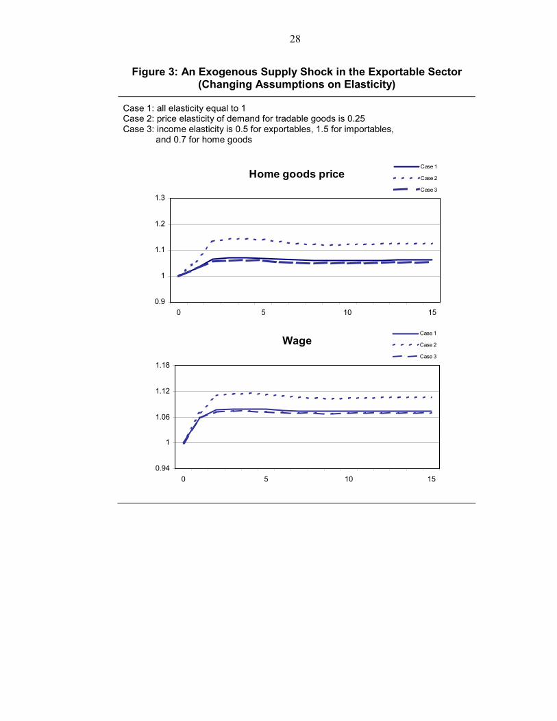
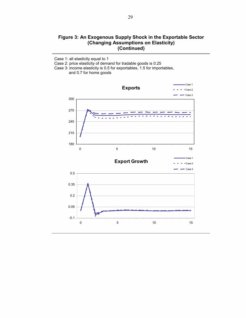
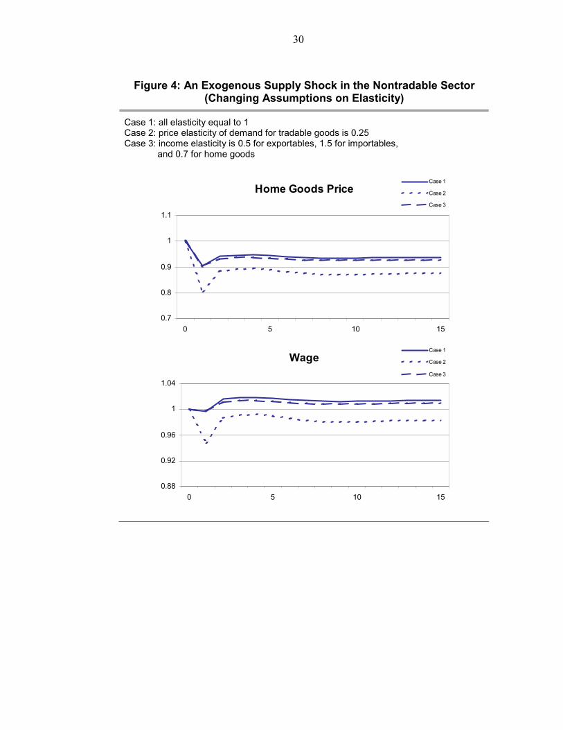
C. Changing Assumptions on Elasticity

Figure 3 and Figure 4 report the movement of some key economic variables towards the new equilibrium after a 50 unit real cost reduction taking place, respectively, in the exportable sector and in the nontradable sector, and compare across cases with different assumptions on elasticity. Case 1 is the benchmark case as described above. In Case 2, the assumption on the price elasticity of demand for tradable goods is changed to be 0.25. In Case 3, the effect of a higher income elasticity for importables is studied. The new income elasticities of demand for exportable, importable, and nontradable are assumed to be 0.5, 1.5, and 0.7. In general, these changes in assumptions do not change the main conclusion that a technological advance in either the exportable or the nontradable may generate high export growth together with high GDP growth. But the magnitude of changes in some economic variables, such as exports and wages, is sensitive to the assumptions on elasticites. In Figure 3 and Figure 4, it is observed that a bigger income elasticity of demand for importables generates a higher export growth. This is consistent with intuition, since exports are used to pay for imports, thus a higher demand for imports stimulated by economic growth generates a bigger increase in exports. Furthermore, in Figure 4, we observe that a price elasticity of demand for tradables of 0.25 generates a higher export growth than the benchmark case. Therefore, as shown in the comparative version, with assumptions of a smaller price elasticity of demand for tradables and a bigger income elasticity of demand for importables, it is more likely that a technological advance taking place in the nontradable sector may generate an export growth that is higher than GDP growth. The real exchange rate, once again, is proven to be a more reliable candidate than the co-occurrence of high export and GDP growth to distinguish between “exports driving growth” and “growth driving exports”.

18

IV. Empirical Evidence

A. Real Exchange Rate Movement in High Growth Periods The model, both in the comparative static version and the dynamic version, shows that the real exchange rate movement is a key factor helping distinguish between a scenario of “exports driving growth” and one of “growth driving exports”. If the growth is initiated by the exportable sector, the real exchange rate appreciates. On the contrary, if the growth is led by the home good sector, the real exchange rate depreciates. As Table 3 indicates, for a total 70 high growth episodes in which exports grew faster than GDP, only half of them experienced real exchange rate appreciation, other 26 experienced depreciation and the remaining nine insignificant changes. This sheds some light on the fact that not all of these high GDP and high export growth cases should be labeled “exports driving growth”. The model suggests that calibrating TFP improvement at sector level may help reveal the true story. However, in many developing countries, data inadequacy does not allow such calibration of TFP at industry level. To further identify the underlying forces behind those high export and high GDP growth episodes, this paper makes use of the model’s conclusion that the real exchange rate helps distinguish between “exports driving growth” and “growth driving exports”. We should recognize, of course, that productivity is not the only factor that determines the real exchange rate. Therefore, labor productivity at the sector level is calibrated, which can be regarded as a good proxy for TFP. If a high export and high GDP growth experiences both a significant real exchange rate appreciation and a significantly faster labor productivity improvement in the tradable than the nontradable sector, such an episode is consistent with the “export-led growth” hypothesis and can be labeled “exports driving growth”. If, on the contrary, a high export and high GDP growth experiences both a significant real exchange rate depreciation and a significant faster labor productivity improvement in the nontradable than the tradable sector, then it is more likely that such episode is one of “growth driving exports” as indicated by the model.

B. Labor Productivity

Data on output and labor input at sector level are available from the United Nation National Accounts Main Aggregates Database (UNNAMAD) and the International Labor Organization (LABORSTA) Database. The distinction between the tradable and the nontradable sector is usually made based on the extent to which the prices are determined in the international market. UNNAMAD and the LABORSTA use different industry classification. The sector breakdown of the tradable and the nontradable sector is in Table 7. Traditional classification is adopted, which classifies agriculture, mining and quarrying, and manufacturing goods as tradable goods while other industries are classified as nontradable. It would be more appropriate to classify the utility industry as nontradable. In UNNAMAD dataset, however, the utility industry is combined and reported together with mining and manufacturing. To be consistent with such

19

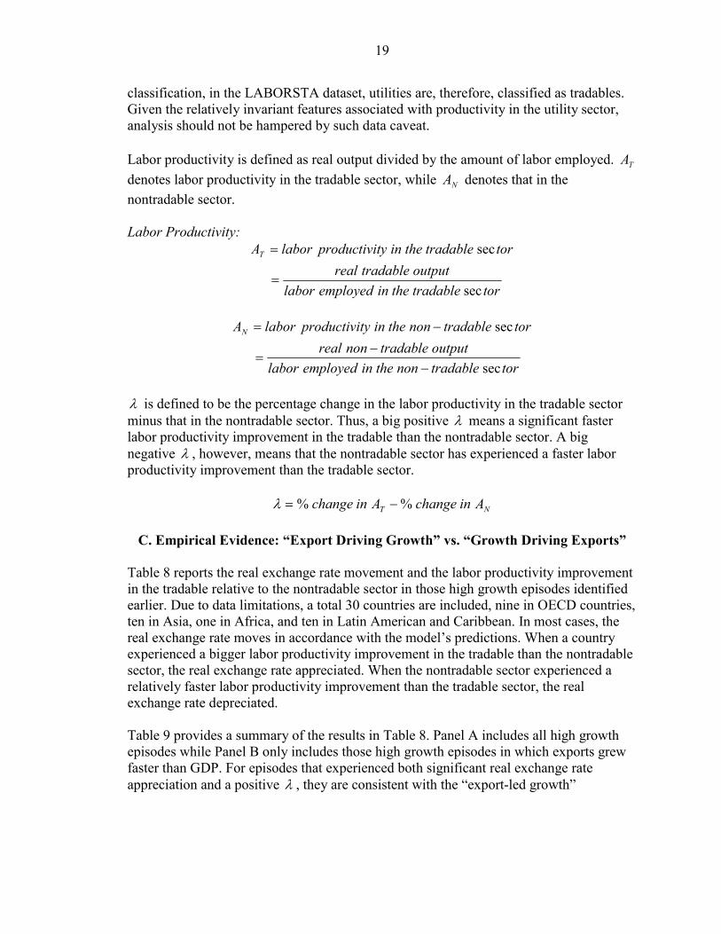
classification, in the LABORSTA dataset, utilities are, therefore, classified as tradables. Given the relatively invariant features associated with productivity in the utility sector, analysis should not be hampered by such data caveat. Labor productivity is defined as real output divided by the amount of labor employed. TA denotes labor productivity in the tradable sector, while NA denotes that in the nontradable sector. Labor Productivity:

tortradabletheinemployedlaboroutputtradablereal

tortradabletheintyproductivilaborAT

sec

sec

=

=

tortradablenontheinemployedlaboroutputtradablenonreal

tortradablenontheintyproductivilaborAN

sec

sec

−−

=

−=

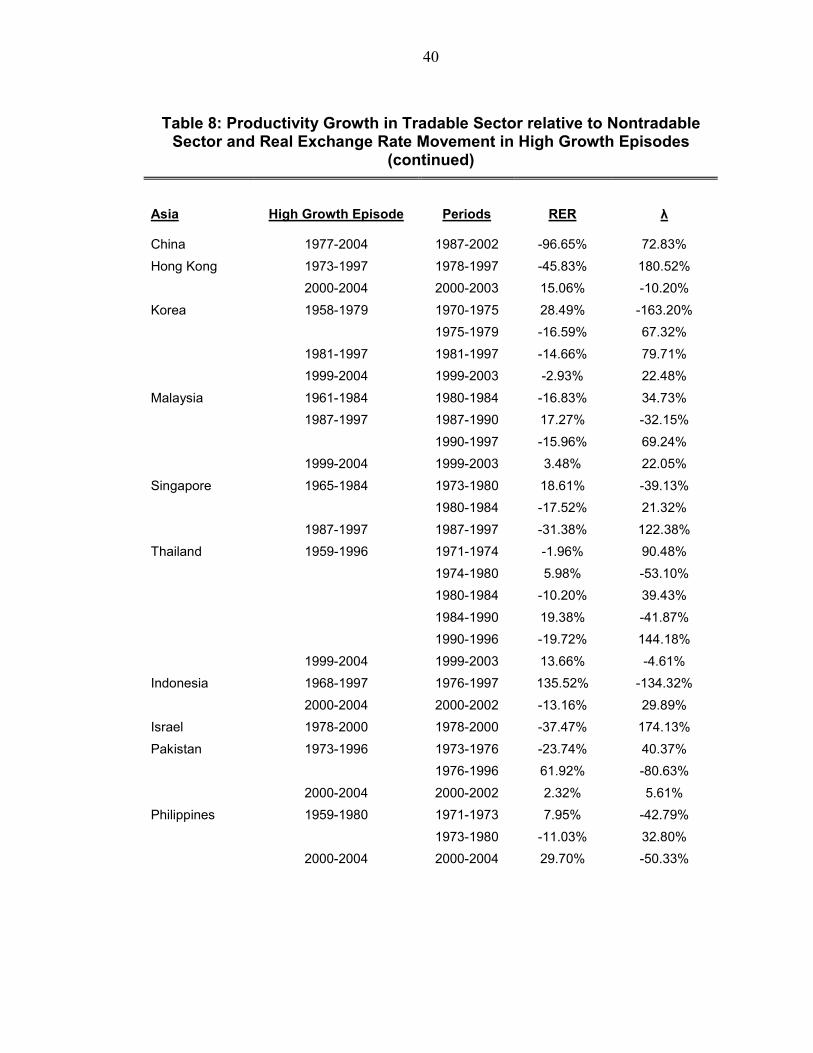
λ is defined to be the percentage change in the labor productivity in the tradable sector minus that in the nontradable sector. Thus, a big positive λ means a significant faster labor productivity improvement in the tradable than the nontradable sector. A big negative λ , however, means that the nontradable sector has experienced a faster labor productivity improvement than the tradable sector.

NT AinchangeAinchange %% −=λ

C. Empirical Evidence: “Export Driving Growth” vs. “Growth Driving Exports”

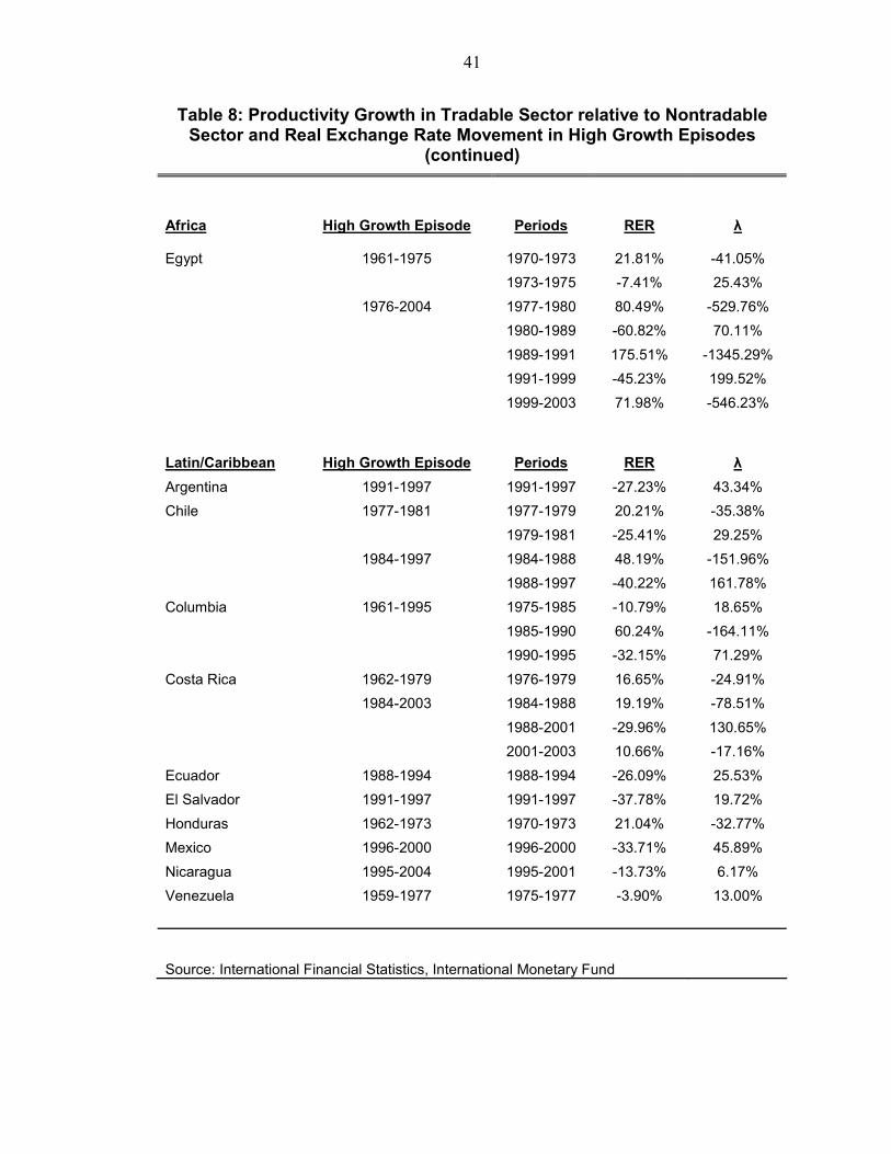
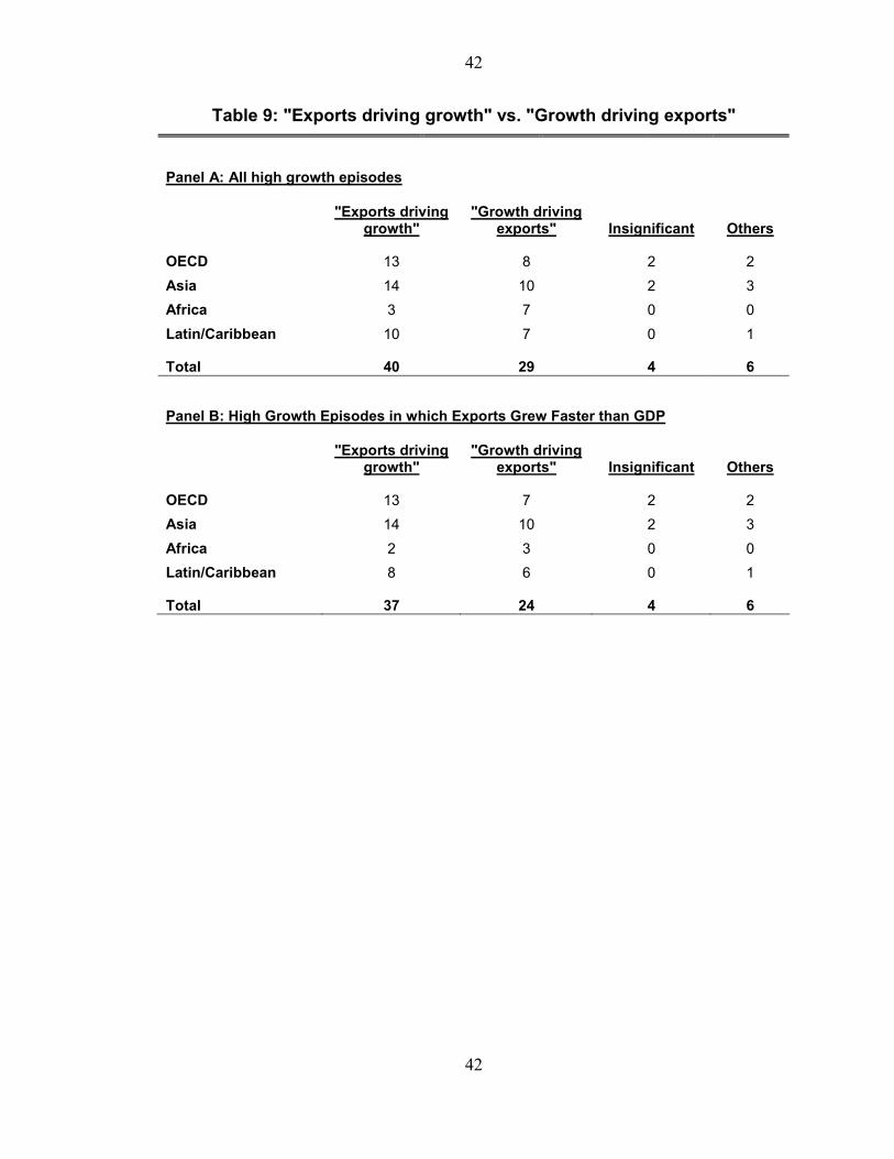
Table 8 reports the real exchange rate movement and the labor productivity improvement in the tradable relative to the nontradable sector in those high growth episodes identified earlier. Due to data limitations, a total 30 countries are included, nine in OECD countries, ten in Asia, one in Africa, and ten in Latin American and Caribbean. In most cases, the real exchange rate moves in accordance with the model’s predictions. When a country experienced a bigger labor productivity improvement in the tradable than the nontradable sector, the real exchange rate appreciated. When the nontradable sector experienced a relatively faster labor productivity improvement than the tradable sector, the real exchange rate depreciated. Table 9 provides a summary of the results in Table 8. Panel A includes all high growth episodes while Panel B only includes those high growth episodes in which exports grew faster than GDP. For episodes that experienced both significant real exchange rate appreciation and a positive λ , they are consistent with the “export-led growth”

20

hypothesis and thus are classified as “exports driving growth”. Such episodes are in accordance with the traditional view that it was usually a technological advance (or an exogenous increase in the main export goods) that led to both high export and high GDP growth. For episodes that experienced both significant real exchange rate depreciation and a negative λ , however, they are more likely to reflect a technological advance in the nontradable sector generating high export growth together with high GDP growth. Thus they are classified as “growth driving exports”. There are some episodes that experienced both an insignificant change in the real exchange rate and a small λ , I classify these as the “Insignificant” group in Table 9. In those episodes, the labor productivity improvement may have been pretty evenly distributed across the tradable and the nontradable sectors. The “Others” group includes those episodes which the change in the real exchange rate and λ is not in accordance to what the model predicts, i.e. cases of significant real exchange rate appreciation together with a negative λ or those of significant real exchange rate deprecation together with a positive λ . In such episodes, some factors other than productivity must have played a dominant role in determining the real exchange rate. Those factors can be capital inflows or outflows, changes in trade policy, people’s taste for exportables or importables, etc. There are, however, only six such cases (out of 79 or 71). It is found that in all 79 high growth episodes, there are only 40 episodes can be labeled as “export-led growth”. There are 29 other episodes that are more likely to be characterized by “growth driving exports”, i.e., the nontradable sector was the main driving force behind such high growth episodes. In Panel B, which only includes episodes that experienced a higher export growth than GDP growth and are thus more likely to be the “export-led growth” story, we see only 37 out of 71 episodes are consistent with the “export-led growth” hypothesis, while a significant portion (24 cases) are more likely to reflect “growth driving exports”. Therefore, Table 9 provides strong empirical evidence to show that the nontradable sector played a very important role in leading high economic growth and high export growth. Many alleged “export-led growth” episodes were actually led by the productivity improvement in the nontradable sector. This conclusion may have important policy implications for developing countries. Looking into history, especially after the successful stories of “Asian Tigers”" in which export booms led economic growth for nearly two decades, the idea of “export-led growth” has encouraged many government to implement various “export-promoting policies”, in the hope of duplicating the success of “Asian Tigers”. Most of those export promotion policies take the forms of subsidies to export activities, devaluation of nominal exchange rate, elimination of import tariffs on imported inputs used in the production of main export goods, etc. However, this paper suggests that productivity in the nontradable sector probably played just as important a role as that in the tradable sector in driving economic growth. “Export-led growth” did not dominate the scene, as many people believed. Countries should, therefore, weight their option before providing special privileges to the export sector. Economic policies that encourage technological

21

improvement in all industries, both tradable and nontradable, such as improving the quality of the population, removing barriers to preventing resources moving more freely to the sectors with a comparative advantage, improving the quality of institutions, etc., appear equally important in driving high economic growth.

V. Conclusion

The lack of evidence of real exchange rate appreciation in many episodes in which both GDP and exports grew dramatically leads to doubts as to how such episodes could appropriately be labeled as “export-led growth”, implying that their main driving force comes from the export sector. The model in this paper shows that productivity improvement in either the tradable or the nontradable sector may result in high economic growth together with even higher export growth. The model also indicates that when TFP is not directly measurable, which is a common data problem in many developing countries, the real exchange rate can serve as a good indicator to distinguish between episodes of “exports driving growth” and those of “growth driving exports”. In episodes of “exports driving growth”, the real exchange rate should appreciate; and in episodes of “growing driving exports”, it should depreciate. People's demand for imports increases, bidding up the real price of foreign currency. This, in turn, stimulates the expansion of the export sector. Thus exports grow in order to pay for the increased imports; exports can grow faster than GDP if the income elasticity of demand for imports is sufficiently high. The data show that among episodes characterized by high GDP growth together with even higher export growth, about half of them are consistent with the “export-led growth” hypothesis; most of the other half was more likely led by productivity improvement in the nontradable sector. Therefore, the conclusion of this paper is that the nontradable sector can play as important a role as the tradable sector in driving episodes in which both GDP and exports grow rapidly.

22

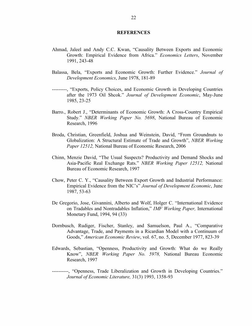
REFERENCES

Ahmad, Jaleel and Andy C.C. Kwan, “Causality Between Exports and Economic Growth: Empirical Evidence from Africa.” Economics Letters, November 1991, 243-48

Balassa, Bela, “Exports and Economic Growth: Further Evidence.” Journal of

Development Economics, June 1978, 181-89 ---------, “Exports, Policy Choices, and Economic Growth in Developing Countries

after the 1973 Oil Shcok.” Journal of Development Economic, May-June 1985, 23-25

Barro., Robert J., “Determinants of Economic Growth: A Cross-Country Empirical

Study.” NBER Working Paper No. 5698, National Bureau of Economic Research, 1996

Broda, Christian, Greenfield, Joshua and Weinstein, David, “From Groundnuts to

Globalization: A Structural Estimate of Trade and Growth”, NBER Working Paper 12512, National Bureau of Economic Research, 2006

Chinn, Menzie David, “The Usual Suspects? Productivity and Demand Shocks and

Asia-Pacific Real Exchange Rats.” NBER Working Paper 12512, National Bureau of Economic Research, 1997

Chow, Peter C. Y., “Causality Between Export Growth and Industrial Performance:

Empirical Evidence from the NIC’s” Journal of Development Economic, June 1987, 53-63

De Gregorio, Jose, Givannini, Alberto and Wolf, Holger C. “International Evidence

on Tradables and Nontradables Inflation,” IMF Working Paper, International Monetary Fund, 1994, 94 (33)

Dornbusch, Rudiger, Fischer, Stanley, and Samuelson, Paul A., “Comparative

Advantage, Trade, and Payments in a Ricardian Model with a Continuum of Goods,” American Economic Review, vol. 67, no. 5, December 1977, 823-39

Edwards, Sebastian, “Openness, Productivity and Growth: What do we Really

Know”, NBER Working Paper No. 5978, National Bureau Economic Research, 1997

----------, “Openness, Trade Liberalization and Growth in Developing Countries.”

Journal of Economic Literature, 31(3) 1993, 1358-93

23

Emery, R.F., “The Relations of Exports and Economic Growth.” Kyklos, 1967, 479-

86 Engle, Robert and David F. Hendry. “Testing Superexogeneity and Invariance in

Regression Models.” Journal of Econometrics, February 1993, 119-39 --------- and --------, and Jean-Francois Richard, “Exogeneity.” Econometric, March

11983, 227-304 Feenstra, Robert, Chi-Yuan Liang, Madani, Dorsati and Yangm Tzu-Han, “Testing

Endogenous Growth in South Korea and Taiwan.” Journal of Development Economics, LX 1999, 317-341

Feder, G., “On Exports and Economic Growth.” Journal of Development Economics,

February- April 1983, 59-73 Frankel, Jeffrey, and Romer, David, “Does Trade Cause Growth?”, American

Economic Review, LXXXIX 1999, 379-399 Giles, D.E.A., J.A. Giles and E. McCann., “Causality, Unit Roots and Export-Led

Growth: The New Zealand Experience.” University of Canterbury Working Paper No. 9206, 1992

Granger, Clive W. J., “Investigating Causal Relations by Econometric Models and

Cross Spectral Models.” Econometrica, July 1969, 4-38 Grossman, Gene and Helpman, Elhanan, “Trade, Innovation, and Growth.” American

Economic Review, LXXX 1990, 86-91 Harberger, Arnold C. “Economic Growth and the Real Exchange Rate: Revisiting the

Balassa-Samuelson Effect,” Prepared for a conference Organized by the higher School of Economics, Moscow, April 2003

-----------, "A Vision of the Growth Process," American Economic Review, American

Economic Association, March 1998, vol. 88(1), 1-32 Hsiao, M. C. W., “Test of Causality and Exogeneity Between Exports and Economic

Growth: the case of Asian NICs.” Journal of Economic Development, December 1987, 143-59

Hsieh, David A. “The Determination of the Real Exchanger Rate: The Productivity

Approach,” Journal of International Economics, 1982, 12, 355-362

24

Ito, Takatoshi, Isard, Pater and Symansky, Steven, “Economic Growth and Real Exchange Rate: An Overview of the Balassa-Samuelson Hypothesis in Asia,” NBER Working Paper, National Bureau Economic Research, 1997

Jung, W.S. and P.J. Marshall, “Exports, Growth and Causality in Developing

Countries.” Journal of Development Economics, May-June 1985, 1-12 Keesing, D. B., “Outward-looking Policies and Economic Development.” Economic

Journal, 1967, 303-20, Kravis, I.B., “Trade as Handmaiden of Growth: Similarities between the Nineteenth

and the Twentieth Centuries.” Economic Journal, 1970, 80, 850-72 Kunst, R. and P. Meguire, “On Exports and Productivity: A Causal Analysis.” The

Review of Economics and Statistics, November 1989, 699-703 Kwan Andy C.C. and John Cotsomitis, “Economic Growth and the Expanding Export

Sector: China 1952-1985.” International Economic Journal, 1991, 105-16 Lee, Jaewoo and Tang, Man-Keung, “Does Productivity Growth lead to Appreciation

of the Real Exchange Rate?” IMF Working Paper, International Monetary Fund, WP/03/154, 2003

Maizels, A., Exports and Growth in Developing Countries, Cambridge and New

York, Cambridge University Press, 1968 Marin, D., “Is the Export-led Growth Hypothesis Valid for the Industrialized

Countries?” Review of Economics and Statistics, 1992, 74, 678-88 Noguer, Marta and Siscart, Marc, “Trade Raises Income: A Precise and Robust

Result.” Journal of International Economics, Vol. 65, Isssue 2, March 2005 Pinic, M. and Rajan, A.H., Product Changes in Industrial Countries Trade: 1955-

1968.” NEDO Monograph No.2, London, 1973 Ram Rati, “Exports and Economic Growth: some Additional Evidence.” Economic

Development and Cultural Change, January 1985, 415-25 -----------, “Exports and Economic Growth in Developing Countries: Evidence from

Time Series and Cross-Section Data.” Economic Development and Cultural Change, January 1987, 51-72

Rivera-Batiz, Luis and Romer Paul, “Economic Integration and Endogenous

Growth.” The Quarterly Journal of Economics, CVI1991, 531-555

25

Rodrigues, Francisco and Rodrik, Dani, “Trade Policy and Economic Growth: A

Skeptics’s Guide to the Cross-National Evidence.” Macroeconomics Annual 2000, eds. Ben Bernanke and Kenneth S. Rogoff, MIT Press for NBER, Cambridge, MA, 2001

State Statistical Bureau. Statistical Yearbook of China, Beijing: China Statistical

Information & Consultancy Tyler, W.B., “Growth and Export Expansion in Developing Countries.” Journal of

Development Economics, August 1981, 121-30 Voivodas, C.S., “Exports, Foreign Capital Inflow and Economic Growth.” Journal of

International Economics, November 1973, 337-349 Yamazawa, I., Economic Development and Internaional Trade – The Japanese

Model, East-West Center, Honolulu, HA, 1990

26

Figure 1: A Technological Advance in the Exportable Sector

Home Goods Price

0.96

1

1.04

1.08

1.12

0 5 10 15

Exports

160

200

240

280

320

0 5 10 15

Wage

0.96

1

1.04

1.08

1.12

0 5 10 15

Real Wage

0.96

1

1.04

1.08

1.12

0 5 10 15

Trade Balance

-20

0

20

40

60

0 5 10 15

International Reserves

80

100

120

140

160

0 5 10 15

Export Growth

-0.15

0

0.15

0.3

0.45

0 5 10 15

Money Supply

400

500

600

700

800

0 5 10 15

27

Figure 2: A Technological Advance in the Nontradable Sector

Home Goods Price

0.85

0.9

0.95

1

1.05

0 5 10 15

Exports

180

190

200

210

220

0 5 10 15

Wage

0.99

1

1.01

1.02

1.03

0 5 10 15

Real Wage

0.96

1

1.04

1.08

1.12

0 5 10 15

Trade Balance

-20

0

20

40

60

0 5 10 15

International Reserves

80

100

120

140

160

0 5 10 15

Export Growth

-0.08

-0.04

0

0.04

0.08

0 2 4 6 8 10 12 14

Money supply

400

500

600

700

800

0 5 10 15

28

Figure 3: An Exogenous Supply Shock in the Exportable Sector (Changing Assumptions on Elasticity)

Case 1: all elasticity equal to 1 Case 2: price elasticity of demand for tradable goods is 0.25 Case 3: income elasticity is 0.5 for exportables, 1.5 for importables, and 0.7 for home goods

Home goods price

0.9

1

1.1

1.2

1.3

0 5 10 15

Case 1

Case 2

Case 3

Wage

0.94

1

1.06

1.12

1.18

0 5 10 15

Case 1

Case 2

Case 3

29

Figure 3: An Exogenous Supply Shock in the Exportable Sector

(Changing Assumptions on Elasticity) (Continued)


Exports

180

210

240

270

300

0 5 10 15

Case 1

Case 2

Case 3

Export Growth

-0.1

0.05

0.2

0.35

0.5

0 5 10 15

Case 1

Case 2

Case 3

30

Figure 4: An Exogenous Supply Shock in the Nontradable Sector

(Changing Assumptions on Elasticity)


Home Goods Price

0.7

0.8

0.9

1

1.1

0 5 10 15

Case 1

Case 2

Case 3

Wage

0.88

0.92

0.96

1

1.04

0 5 10 15

Case 1

Case 2

Case 3

31

Figure 4: An Exogenous Supply Shock in the Nontradable Sector

(Changing Assumptions on Elasticity) (Continued)


Exports

165

180

195

210

225

0 5 10 15

Case 1

Case 2

Case 3

Export Growth

-0.1

-0.05

0

0.05

0.1

0 5 10 15

Case 1

Case 2

Case 3

32

Table 1: GDP and Export Growth in High Growth Episodes

OECD Countries Period GDP Growth Export Growth

Australia 1962-1981 4.21% 5.64% 1984-1989 4.62% 7.12% 1994-2002 4.03% 4.81% Canada 1962-1976 4.99% 7.80% 1984-1988 4.45% 4.69% 1994-2000 4.05% 9.37% France 1959-1973 5.83% 9.20% Finland 1961-1973 5.03% 9.23% 1995-2000 4.61% 7.08% Greece 1958-1973 7.21% 11.90% 2000-2004 4.40% 7.02% Ireland 1959-1978 4.62% 8.68% 1984-2004 6.04% 11.21% Japan 1958-1964 9.90% 13.28% 1966-1973 9.42% 14.04% 1976-1990 4.24% 5.83% New Zealand 1958-1965 4.70% 4.59% 1969-1974 4.49% 6.10% Norway 1967-1985 4.15% 6.12% Portugal 1967-1973 10.94% 10.57% 1976-1980 5.37% 4.67% 1986-1990 4.70% 15.73% Spain 1958-1974 6.39% 16.35% 1995-2000 4.27% 8.28%

33


(Continued) Asia Period GDP Growth Export Growth China 1969-1975 9.43% 9.47% 1977-2004 9.44% 13.55% Hong Kong 1973-1997 7.15% 11.69% 2000-2004 4.76% 4.55% Korea 1958-1979 7.82% 23.55% 1981-1997 8.01% 11.29% 1999-2004 6.09% 7.95% Malaysia 1961-1984 7.28% 7.34% 1987-1997 8.92% 14.63% 1999-2004 5.31% 6.19% Singapore 1965-1984 9.77% 11.93% 1987-1997 9.08% 13.95% Thailand 1959-1996 7.79% 10.89% 1999-2004 4.98% 6.19% India 1958-1964 5.12% 5.15% 1980-2003 5.74% 7.21% Indonesia 1968-1997 6.93% 13.92% 2000-2004 4.63% 6.57% Israel 1978-2000 5.59% 6.88% Pakistan 1960-1969 4.96% 5.51% 1973-1996 5.75% 9.23% 2000-2004 4.10% 6.60% Philippines 1959-1980 5.31% 9.19% 2000-2004 4.57% -1.25% Africa Period GDP Growth Export growth Cameroon 1968-1986 6.33% 11.56% Egypt 1961-1975 4.81% 4.29% 1976-2004 5.82% 5.98% Morocco 1967-1971 6.12% 3.69% South Africa 1962-1974 5.38% 6.65%

34

Table 1: GDP and Export Growth in High Growth Episodes (Continued)

Latin/Caribbean Period GDP growth Export growth Argentina 1968-1974 4.74% 14.41% 1991-1997 6.08% 10.62% Brazil 1965-1980 8.81% 10.52% Chile 1961-1971 4.69% 1.37% 1977-1981 7.51% 7.06% 1984-1997 7.21% 9.25% Columbia 1961-1995 4.70% 4.80% Costa Rica 1962-1979 6.55% 7.80% 1984-2003 4.73% 8.72% Ecuador 1967-1980 7.88% 14.51% 1988-1994 4.16% 5.98% Guatemala 1958-1979 5.46% 7.54% 1992-1998 4.30% 11.38% El Salvador 1958-1978 5.24% 6.10% 1991-1997 6.75% 18.37% Honduras 1962-1973 5.21% 7.56% 1984-1989 4.04% 8.26% Jamaica 1964-1972 6.15% 5.51% Mexico 1958-1981 6.73% 8.58% 1996-2000 5.46% 17.98% Nicaragua 1961-1974 6.75% 9.05% 1995-2004 4.22% 8.51% Paraguay 1961-1981 6.87% 7.45% Peru 1960-1981 4.96% 6.19% 1993-1997 7.10% 12.91% Uruguay 1975-1980 4.74% 7.09% 1986-1994 4.56% 7.55% Venezuela 1959-1977 5.94% 5.61%

Source: International Financial Statistics, IMF

35


Export Growth Export Growth > GDP Growth < GDP Growth

OECD 21 3 Asia 22 2 Africa 3 2 Latin & Caribbean 24 4

Total 70 11


Table 3: Real Exchange Rate Movement in High Growth Episodes

(All High Growth Episodes)

Appreciation Depreciation Insignificant

OECD 15 6 3 Asia 9 13 2 Africa 1 3 1 Latin & Caribbean 14 11 3

Total 39 33 9

(High Growth Episodes in which Exports Grew Faster than GDP)

Appreciation Depreciation Insignificant

OECD 13 5 3 Asia 9 11 2 Africa 1 1 1 Latin & Caribbean 12 9 3

Total 35 26 9


36

Table 4: Changes in the Equilibrium Home Goods Price and in Wages

(A 50 Unit Real Cost Reduction in the Exportable Sector)

Initial GDP = 1,000 Case 1: all income elasticity =1

exη imη New hP New w GDP growth Export Growth 1 1 1.062 1.074 5% 29.76% 1 0.5 1.084 1.085 5% 26.95%

0.5 0.5 1.093 1.089 5% 28.22% 0.3 0.5 1.097 1.091 5% 28.79% 0.3 0.3 1.116 1.101 5% 27.05% 0.2 0.2 1.133 1.109 5% 26.23%

Case 2: income elasticity: 0.5 for exportables, 1.5 for importables, 0.7 for home goods


0.5 0.5 1.078 1.082 5% 30.96% 0.3 0.5 1.081 1.083 5% 31.45% 0.3 0.3 1.097 1.092 5% 29.99% 0.2 0.2 1.111 1.098 5% 29.30%

37

Table 5: Changes in the Equilibrium Home Goods Price and in Wages

(A 50 Unit Real Cost Reduction in the Home Goods Sector)

Initial GDP = 1,000 Case 1: all income elasticity =1

exη imη New hP New w GDP growth Export Growth 1 1 0.936 1.014 5% -1.36% 1 0.5 0.913 1.002 5% 1.53%

0.5 0.5 0.905 0.998 5% 0.23% 0.3 0.5 0.901 0.996 5% -0.37% 0.3 0.3 0.881 0.986 5% 1.42% 0.2 0.2 0.864 0.977 5% 2.27%



0.5 0.5 0.89 0.99 5% 2.98% 0.3 0.5 0.885 0.988 5% 2.29% 0.3 0.3 0.862 0.976 5% 4.36% 0.2 0.2 0.842 0.967 5% 5.34%



0.5 0.5 0.87 0.98 5% 4.98% 0.3 0.5 0.864 0.978 5% 4.16% 0.3 0.3 0.837 0.964 5% 6.61% 0.2 0.2 0.814 0.952 5% 7.77%

38

Table 6: Summary of Model Results

Technological advance taking place in The tradable sector The nontradable sector Exports Grow Grow/Not Grow GDP Grow Grow Real wage Increase Increase Real exchange rate Appreciate Depreciate

Table 7: Industrial Classification of Tradable and Nontradable Sector

The United Nations National Accounts

Tradable 1) Agriculture, hunting, forestry, fishing 2) Mining, Manufacturing, Utilities 3) Manufacturing

Nontradable 4) Construction 5) Wholesale, retail trade, restaurants and hotels 6) Transport, storage and communication 7) Other activities International Labor Organization Database

Tradable 1) Agriculture, Hunting, Forestry and Fishing 2) Mining and Quarrying 3) Manufacturing 4) Electricity, Gas and Water

Nontradable 5) Construction 6) Wholesale and Retail Trade and Restaurants and Hotels 7) Transport, Storage and Communication 8) Financing, Insurance, Real Estate and Business Services 9) Community, Social and Personal Services 10) Activities not Adequately Defined Source: the United Nations Database and the International Labor Organization Database

39

Table 8: Productivity Growth in Tradable Sector relative to Nontradable Sector and Real Exchange Rate Movement in High Growth Episodes

OECD Countries High Growth Episode Periods RER λ

Australia 1962-1981 1970-1973 -13.64% 38.01% 1973-1980 17.18% -21.57% 1980-1981 -9.14% 15.29% 1984-1989 1984-1986 19.59% -33.93% 1986-1989 -17.28% 29.66% 1994-2002 1994-1997 -7.91% 13.99% 1997-2002 15.11% -18.46% Canada 1962-1976 1970-1975 14.35% -10.14% 1975-1976 -7.69% 9.94% 1984-1988 1984-1988 2.82% 0.55% 1994-2000 1994-2000 -2.77% 22.07% Finland 1961-1973 1970-1973 -3.24% 21.77% 1995-2000 1995-2000 24.75% -13.29% Greece 2000-2004 2000-2003 -22.56% 36.48% Ireland 1984-2004 1984-2003 -36.79% 405.27% Japan 1966-1973 1970-1973 -18.36% 58.16% 1976-1990 1976-1978 -22.97% 54.32% 1978-1980 27.31% -49.20% 1980-1990 -31.26% 100.45% Norway 1967-1985 1972-1977 -14.56% 61.61% 1977-1985 18.33% 16.01% Portugal 1976-1980 1976-1980 19.06% -15.46% 1986-1990 1986-1990 -19.83% 68.96% Spain 1958-1974 1970-1974 -14.42% 112.99% 1995-2000 1995-2000 15.95% -17.74%

40

Table 8: Productivity Growth in Tradable Sector relative to Nontradable

Sector and Real Exchange Rate Movement in High Growth Episodes (continued)

Asia High Growth Episode Periods RER λ

China 1977-2004 1987-2002 -96.65% 72.83% Hong Kong 1973-1997 1978-1997 -45.83% 180.52% 2000-2004 2000-2003 15.06% -10.20% Korea 1958-1979 1970-1975 28.49% -163.20% 1975-1979 -16.59% 67.32% 1981-1997 1981-1997 -14.66% 79.71% 1999-2004 1999-2003 -2.93% 22.48% Malaysia 1961-1984 1980-1984 -16.83% 34.73% 1987-1997 1987-1990 17.27% -32.15% 1990-1997 -15.96% 69.24% 1999-2004 1999-2003 3.48% 22.05% Singapore 1965-1984 1973-1980 18.61% -39.13% 1980-1984 -17.52% 21.32% 1987-1997 1987-1997 -31.38% 122.38% Thailand 1959-1996 1971-1974 -1.96% 90.48% 1974-1980 5.98% -53.10% 1980-1984 -10.20% 39.43% 1984-1990 19.38% -41.87% 1990-1996 -19.72% 144.18% 1999-2004 1999-2003 13.66% -4.61% Indonesia 1968-1997 1976-1997 135.52% -134.32% 2000-2004 2000-2002 -13.16% 29.89% Israel 1978-2000 1978-2000 -37.47% 174.13% Pakistan 1973-1996 1973-1976 -23.74% 40.37% 1976-1996 61.92% -80.63% 2000-2004 2000-2002 2.32% 5.61% Philippines 1959-1980 1971-1973 7.95% -42.79% 1973-1980 -11.03% 32.80% 2000-2004 2000-2004 29.70% -50.33%

41

Table 8: Productivity Growth in Tradable Sector relative to Nontradable Sector and Real Exchange Rate Movement in High Growth Episodes

(continued)

Africa High Growth Episode Periods RER λ

Egypt 1961-1975 1970-1973 21.81% -41.05% 1973-1975 -7.41% 25.43% 1976-2004 1977-1980 80.49% -529.76% 1980-1989 -60.82% 70.11% 1989-1991 175.51% -1345.29% 1991-1999 -45.23% 199.52% 1999-2003 71.98% -546.23%

Latin/Caribbean High Growth Episode Periods RER λ Argentina 1991-1997 1991-1997 -27.23% 43.34% Chile 1977-1981 1977-1979 20.21% -35.38% 1979-1981 -25.41% 29.25% 1984-1997 1984-1988 48.19% -151.96% 1988-1997 -40.22% 161.78% Columbia 1961-1995 1975-1985 -10.79% 18.65% 1985-1990 60.24% -164.11% 1990-1995 -32.15% 71.29% Costa Rica 1962-1979 1976-1979 16.65% -24.91% 1984-2003 1984-1988 19.19% -78.51% 1988-2001 -29.96% 130.65% 2001-2003 10.66% -17.16% Ecuador 1988-1994 1988-1994 -26.09% 25.53% El Salvador 1991-1997 1991-1997 -37.78% 19.72% Honduras 1962-1973 1970-1973 21.04% -32.77% Mexico 1996-2000 1996-2000 -33.71% 45.89% Nicaragua 1995-2004 1995-2001 -13.73% 6.17% Venezuela 1959-1977 1975-1977 -3.90% 13.00%

Source: International Financial Statistics, International Monetary Fund

42

42

Table 9: "Exports driving growth" vs. "Growth driving exports"

Panel A: All high growth episodes

"Exports driving

growth" "Growth driving

exports" Insignificant Others

OECD 13 8 2 2 Asia 14 10 2 3 Africa 3 7 0 0 Latin/Caribbean 10 7 0 1

Total 40 29 4 6 Panel B: High Growth Episodes in which Exports Grew Faster than GDP

"Exports driving

growth" "Growth driving

exports" Insignificant Others

OECD 13 7 2 2 Asia 14 10 2 3 Africa 2 3 0 0 Latin/Caribbean 8 6 0 1

Total 37 24 4 6

An Analysis of So-Called Export-led Growth; Jie Yang; IMF Working

Documents