An algebraic multigrid solver for transonic flow problems

This article appeared in a journal published by Elsevier. The attachedcopy is furnished to the author for internal non-commercial researchand education use, including for instruction at the authors institution

and sharing with colleagues.

Other uses, including reproduction and distribution, or selling orlicensing copies, or posting to personal, institutional or third party

websites are prohibited.

In most cases authors are permitted to post their version of thearticle (e.g. in Word or Tex form) to their personal website orinstitutional repository. Authors requiring further information

regarding Elsevier’s archiving and manuscript policies areencouraged to visit:

http://www.elsevier.com/copyright

http://www.elsevier.com/copyright

Author's personal copy

An algebraic multigrid solver for transonic flow problems

Shlomy Shitrit a,⇑, David Sidilkover a, Alexander Gelfgat b

a Soreq NRC, Propulsion Physics Laboratory, Yavne 81800, Israelb School of Mechanical Engineering, Faculty of Engineering, Tel-Aviv University, Israel

a r t i c l e i n f o

Article history:Received 29 July 2010Received in revised form 17 November 2010Accepted 22 November 2010Available online 1 December 2010

Keywords:Algebraic multigrid (AMG)Transonic flowFull potential equation

a b s t r a c t

This article presents the latest developments of an algebraic multigrid (AMG) based on fullpotential equation (FPE) solver for transonic flow problems with emphasis on advancedapplications. The mathematical difficulties of the problem are associated with the fact thatthe governing equation changes its type from elliptic (subsonic flow) to hyperbolic (super-sonic flow). The flow solver is capable of dealing with flows from subsonic to transonic andsupersonic conditions and is based on structured body-fitted grids approach for treatingcomplex geometries. The computational method was demonstrated on a variety of prob-lems to be capable of predicting the shock formation and achieving residual reduction ofroughly an order of magnitude per cycle both for elliptic and hyperbolic problems, throughthe entire range of flow regimes, independent of the problem size (resolution).

� 2010 Elsevier Inc. All rights reserved.

1. Introduction

One of the major early breakthroughs in potential flow computation was the work by Murman and Cole on numericalsolution of the small disturbances equation for transonic flow [1]. Their paper laid the ground work for the years that follow.Research on potential flow thrived throughout the 1970s and into the early 1980s. It was a period of rapid development andvarious improvements of potential flow solvers, by numerous researchers. This direction was abandoned, however, whilestill being in its infancy in favor of the Euler and Navier–Stokes solvers. Development of such solvers together with advance-ments in the computer hardware made solving the Navier–Stokes equations practical even for rather complex configura-tions. It looks tough, for some time (more than a decade) that the further development of this methodology, especiallywith regard to efficiency improvement reached a certain stagnation. A substantial departure from the existing methodologymay be required in order to facilitate further progress. One of such possible directions originates from the recommendationby Brandt [2], that since the system of equations is of the mixed type, it is beneficial in terms of efficiency to address each ofthe co-factors separately instead of treating the whole system in the same way. This idea was successfully realized in thepast for the incompressible high Reynolds number flow equations (see for instance [3]), but the progress towards applyingit to the compressible flow was rather slow and the success is very limited. The explanation for this is in the complexity ofthe issues that need to be resolved. One such difficulty is that the standard discretization schemes in multidimensions intro-duce non-physical coupling between the different co-factors of the system. This difficulty is addressed by the emerging classof the so-called factorizable methods [4]. In this light the task of constructing an efficient FPE solver attains a great impor-tance, since such a solver can be used not only by itself, but becomes an integral part of the overall methodology for solvingthe flow equations based upon the factorizable discretization. Potential flow analysis still plays an important role in aircraftdesign and optimization because of its simplicity and efficiency [5].

0021-9991/$ - see front matter � 2010 Elsevier Inc. All rights reserved.doi:10.1016/j.jcp.2010.11.034

⇑ Corresponding author. Tel.: +972 8 9434853; fax: +972 8 9434227.E-mail address: [email protected] (S. Shitrit).

Journal of Computational Physics 230 (2011) 1707–1729

Contents lists available at ScienceDirect

Journal of Computational Physics

journal homepage: www.elsevier .com/locate / jcp


One of the first multilevel methods toward solving partial differential equations fast and efficiently was the multigridmethod [6,7] which was first introduced by Fedorenko [8] in 1964. Other mathematicians extended Fedorenko’s idea to gen-eral elliptic boundary value problems with variable coefficients; see e.g., [9]. However, the full efficiency of the multigridapproach was realized in the works of Brandt [10,11]. He also introduced the modification of multigrid methods for nonlin-ear problems – Full Approximation Scheme (FAS) [11,12]. Another achievement in the formulation of multigrid methods wasthe full multigrid (FMG) scheme [11,12], based on the combination of nested iteration techniques and multigrid methods.

In geometric ‘‘standard’’ multigrid methods the coarse-grids are uniformly coarsened or semi-coarsened, thus the free-dom in the selection of the coarse-grids is limited. The grids hierarchy is constructed based on the grid geometry informationrather than properties of the differential operator. In addition, the definition of smoothness of the error involves grid geom-etry. This geometric dependency imposes certain limits on types of the problems it can be used to solve. For problems withgeneral anisotropies (such anisotropies may occur not only as a property of the operator itself but also as a result of a gridconfiguration) a construction of an efficient geometric multigrid method may become rather cumbersome task. In the 1980salgebraic multigrid (AMG) methods were developed [13–16] to address these issues by extending the main ideas of geomet-ric multigrid methods to an algebraic setting. AMG is a method for solving algebraic systems based on multigrid principleswith no explicit reliance upon the grid geometry. It uses the matrix’s properties only to construct the operators involved inthe algorithm. The AMG framework usually employs a simple pointwise relaxation method whose role is to smooth (in thealgebraic sense) error and then attempts to correct the algebraically smooth error that remains after relaxation by a coarse-level correction.

The purpose of this research is to develop a FPE solver which is based on the AMG method. The previous results werereported in [17] while using the same mathematical basis for solving elementary applications (such as flow around a cylin-der, channel with a bump). The emphasis of this paper is on the more advanced applications. The practical goal of this istwofold: First, to develop an important building block for the factorizable methodology. Second, to develop a stand-alone‘‘optimally’’ efficient FPE solver. The flow solver is to be capable to deal with flow ranging from subsonic to transonic andsupersonic regimes. It can be especially useful for engineers during the design process where multiple computationsneed to be performed as small changes to the geometry are made. The paper is organized as follows: The discretizationof the FPE presented in Section 2. The extensions of the AMG method to the transonic flow computations are discussed inSection 3. In Section 4, several applications for body-fitted structured grids are presented and convergence results for variousflow speeds are given.

2. The FPE discretization

Transonic flow can be described by the full potential equation (FPE) which is derived from the Euler equations by assum-ing that the flow is inviscid, isentropic, and irrotational. The FPE in the conservation form reads as follows:

@

@xðquÞ þ @

@yðqvÞ ¼ 0; ð1Þ

where u and v are the velocity components in the Cartesian coordinates x and y, respectively, and q is the density. The veloc-ity components are given by the gradient of the potential /,

u ¼ @/@x

; v ¼ @/@y

: ð2Þ

The density q is computed from the isentropic formula:

qq1¼ 1þ c� 1

2V21 � /2

x � /2y

� �� 1c�1

; ð3Þ

where c is the ratio of specific heats and V1 is the free-stream velocity and q1 is the free-stream density. The relation be-tween the local speed of sound a and the flow speed is defined by Bernoulli’s equation:

a ¼ a21 �

c� 12

V21 � /2

x � /2y

� �� : ð4Þ

The discretization of the FPE in the conservation form is based on the same rationale that was applied to the quasi-linearform of the equation. For this purpose we address the reader to our previous work [18] while in this section we shall onlybriefly review the general idea.

The strategy of discretizing the FPE in the conservation form is based upon an idea similar to that of the rotated differenceapproach introduced by Jameson [19] and implemented initially in the quasi-linear form. However, this approach is notmade directly. Instead it is accomplished indirectly by following the same rationale.

We review briefly our approach starting with the FPE in the quasi-linear form,

r2/�M21@2

@s2 / ¼ 0; ð5Þ

1708 S. Shitrit et al. / Journal of Computational Physics 230 (2011) 1707–1729


where M1 is free-stream Mach number M1 ¼ V1a1

� �and s-axis denotes the flow direction. Let us look at both the terms from a

numerical standpoint. Note, that when M1 is close to zero (incompressible flow) the second term can be neglected and weare left with Laplacianr2/ which is discretized by certain type of central differencing, according to [18]. As the Mach num-ber increases, the second term, which describes the potential second derivative in the streamwise direction, actually deter-mines the ‘‘dynamics’’ of the flow. When the flow is subsonic, a central difference is used for the second derivative in the flowdirection (/ss), while pointwise relaxation is applied directly in conjunction with the matrix A (or operator L). If the flow issupersonic, we apply relaxation directly with the product of downwind and upwind operators LeL (or matrix AeA), as is de-tailed in our previous work [18]. We would like to apply the same rationale to the discretization of the FPE in the conser-vation form, while the advantages that were obtained in the quasi-linear case discretization, would be implemented.Expanding the FPE and rearranging terms, (5) can be reformulated as,

qr2/þ /x@

@xþ /y

@

@y

� �q ¼ 0; ð6Þ

where the density q is given in (3). Note that (5) and (6) have a similar structure. The density parameter q plays two func-tions. In the first term it serves as a coefficient. In the second term it serves as a variable. As one can see, the second terms inboth of the above equations are identical. For the first term r2/, the fluxes are computed by a central discretization inde-pendent on the flow’s speed. The dynamics of the flow is reflected in the second term which is discretized in such a way thatthe results is a ‘‘wide’’ approximation in the streamwise direction. The flux at given face is a product of the flow velocityvector and the density which are both functions of the potential /. The type of the discretization approach, central fluxesor upwind fluxes, is determined by the local Mach number across the cell’s face. For further details we refer the reader to[20].

3. Classical AMG

In this paper we assume the reader to have some basic knowledge of the ‘‘traditional’’ geometric multigrid. He should befamiliar with smoothing and coarse-grid correction and with the recursive definition of multigrid cycles. We limit our dis-cussion to the basic principles of the AMG method and shall give here a brief description of the classical AMG in the spirit ofStueben [15] followed by a description of the solution process. Regarding more detailed information on geometric and alge-braic multigrid relevant to this work, we also refer to [21,18] and the extensive list of references given therein. We addressthe reader to [15,22,23] for a detailed description of the AMG algorithm, while in this paper we shall only briefly review thealgorithm emphasizing its aspects that require special treatment for the purpose of this work.

Consider a certain boundary-value problem for a scalar PDE in domain X. Its discretization will result in a linear algebraproblem of the form Au = f, where A is an n � n matrix with entries aij with i = 1, . . . ,n, j = 1, . . . ,n, u = {uj} is the vector of un-knowns, b = {bj} is the forcing term vector and n is the number of points in the computational grid covering the domain.

In geometric multigrid the definition of smoothness of the error involves grid geometry. The absence of grids in the AMGcontext renders this definition meaningless. Therefore, the concept of smoothness has to be generalized to some meaningfulmeasurable quantity, which can be computed based on the discrete operator only. An error is algebraically smooth if it isslow to converge with respect to the fine level. Therefore, this smooth error has to be approximated on a coarser level inorder to improve the convergence. Consequently, the coarse-grid correction must deal with the remaining slow components.The characterization of such slow components, e, is: Ae ’ 0.

3.1. Smoothing

Usually, the relaxation used as an ingredient of an AMG algorithm is a pointwise one. One of the central contributions ofour approach is developing a stable pointwise direction-independent relaxation for the entire range of the flow speed, fromlow Mach number flow up until transonic and supersonic regimes. This development was a prerequisite for consideringapplication of AMG to the transonic flow problem. For further details we refer the reader to [18].

3.2. Measuring the algorithm efficiency

The computational complexity concept is intended to measure the algorithm’s requirements for computer resources:computer storage (memory), and CPU time. There are three types of complexity measure that are commonly considered:convergence rate, grid complexity, and operator complexity.

Convergence factor: the rate in which the residual is decreased between consecutive V-cycles. This parameter gives anindication of how many iterations are needed in order to reduce the residual to a sufficient level.Grid complexity: is the total number of elements in the coarse-levels divided by the number of elements on the fine-level.The grid complexity provides a direct measure for the storage required for the solution and right hand side vectors and itis a useful tool to compare different coarsening strategies.

S. Shitrit et al. / Journal of Computational Physics 230 (2011) 1707–1729 1709


Operator complexity: is defined as the sum of the number of nonzero matrix elements in all the coarse-levels, divided bythe number of the nonzero matrix elements on the fine-level. The amount of work required by the relaxation and residualcomputations is directly proportional to the number of the nonzeros on the coarse-levels. Therefore, low value of theoperator complexity that increase linearly with the problem’s resolution signifies a linear complexity operator.

4. Improved AMG components for transonic flow computations

4.1. Dynamic threshold

In the context of an algebraic multigrid we are going to deal at each level with a linear system of equations

Amum ¼ f m; ð7Þ

where m is the level index. The coarsening process is derived based on the strong and weak connections between unknowns,which essentially measures the relative size of the off-diagonal entries. Connections between neighboring variables are con-sidered strong if the size of the corresponding matrix entry exceeds a certain threshold, relative to the maximum entry of therow. This threshold value is very important for constructing a good coarse-grid. According to Ref. [15] a point i is said to bestrongly connected to point j, if

�amij P e max

k–i�am

ik

� �: ð8Þ

The threshold value e is kept fixed for most applications, with a typical value of 0.25. It is well-known that devising a robustcoarsening process, which results in an accurate interpolation, is one of the keys for achieving a good AMG convergence.There are special cases, for example, anisotropic elliptic problems (anisotropy can be a result of the computational grid orthe equation itself), or problems where the equation changes type from elliptic to hyperbolic (transonic flow problem) thata fixed threshold parameter can result in an inadequate coarsening process.

A problem under consideration (supersonic case, for instance) usually leads to a matrix with significant negative off-diag-onal entries. Therefore, it is important to redefine the definition of strong and weak connections, so that it becomes moreadequate for our case. We would like to allow a connection with a negative coefficient, whose absolute value is sufficientlylarge, to be classified as a strong one. Therefore, as it was suggested in [24], we modify the definition (8): a point i is con-sidered to be strongly connected to j if

amij

�� P emaxk–i

amik

�� : ð9Þ

Our further generalization of this idea is to select strong connections using a different threshold parameter for each row ofthe matrix Am, while computing its value by analyzing this row’s entries. Each row represents a difference operator at a spe-cific grid point and, possibly, boundary conditions. Intuitively speaking, the same fixed threshold value (as used in the clas-sical AMG) cannot reflect the relative size of the row’s entries for various cases (isotropic, strongly anisotropic, orhyperbolic). Therefore, in order to maintain a good AMG performance across the entire variety of flow speeds, we proposeto compute the threshold adaptively ‘‘on the fly’’ for each row of the matrix.

Let us define a set of points which are strongly connected to i by Si. Let Nmi ¼ fj 2 Xm : j – i; am

ij – 0g denote the neighbor-hood of a point i 2Xm. Di ¼ Nm

i � Ci; Dsi ¼ Di \ Si; Dw

i ¼ Di � Dsi . The neighboring coarse grid points are denoted by Ci, and the

computational domain is denoted by X. Assuming the operator Am is known, we start from the following equation:

amii um

i þXj2Nm

i

amij um

j ¼ f mi 8i 2 Xm: ð10Þ

Let us define the threshold parameter ei for each row i as

ei ¼P

j–ijaijjjaij j

maxk–i jaik jPj–ijaijj

: ð11Þ

As one can see, the threshold parameter is simply the average value in a given row. Several observations relating to the con-stant-coefficient case are in order here. If a periodic boundary condition is applied, the matrix Am is composed of identicalrows and the threshold parameter can be calculated once for each coarse-level. But, while applying other boundary condi-tions (Dirichlet, Neumann), as for a general problem, it is necessary to calculate the threshold for each row separately.

4.2. The coarse-level and restriction operators

In the classical approach, suggested by Ruge and Stueben, the restriction operator is defined as the transpose of the inter-polation, Imþ1

m ¼ Immþ1

T . Then the coarse-grid operator is defined by the Galerkin-type algorithm, Amþ1 ¼ Imþ1m AmIm

mþ1. We shallrefer, following [24], to this approach as Algorithm 1.

Although this is the simplest way to construct the restriction and coarse-grid operators, it leads to poor convergencewhen the matrix Am is not an M-matrix.



Alternatively, a second algorithm discussed in [24] is to use direct approximations based on the fine grid operator Am toconstruct Am+1 and Imþ1

m . Assuming the operator Am is known, we start from the following equation:

amii um

i þXj2Cm

i

amij um

j þXj2Dm

i

amij um

j � f mi i 2 Cm: ð12Þ

In order to derive the coarse-grid operator Am+1, the terms associated with umj ; j 2 Dm, in the ith equation, i 2 Cm, should be

approximated. The simplest way to account for these elements is to distribute their values among the entries correspondingto strong connections in this row. The resulting coarse-level operator may not always provide in this case a sufficiently accu-rate correction to a fine level solution that in its turn, would lead to poor convergence rates. Alternatively the termsum

j ; j 2 Dm, in the ith equation can be replaced by the jth equation. This operation does not eliminate all umj ; j 2 Dm, but re-

duces magnitudes of their coefficients. Then umj ; j 2 Dm are eliminated by the interpolation formula if jam

ij =amii j 6 ec , or, again,

are replaced by the means of the jth equation when jamij =am

ii j > ec , where ec > 0 is a small number, i.e.,

umj ¼

Pk2Cm

j

wjkumk ; if am

ij =amii

�� 6 ec

f mj

amjj� 1

amjj

Pk2Nm

j

amjkum

k ; if amij =am

ii

�� > ec

8>>><>>>: : ð13Þ

The new equations are obtained

að2Þii umi þ

Xj2Cm

i

að2Þij umj þ

Xj2Dm

i

að2Þij umj � f m

i �Xj2Dm

1

amij

amjj

f mj ; i 2 Cm; ð14Þ

where Dm1 ¼ j : jam

ij =amii j > ec; j 2 Dm

n o. This process is repeated until um

j ; j 2 Dm is eliminated from the ith equation. Therefore,

aðLÞii umi þ

Xj2Cm

i

aðLÞij umj � f m

i �Xj2Dm

1

amij

amjj

f mj ; i 2 Cm; ð15Þ

where að1Þij ¼ amij ;D

ml ¼ j : jaðlÞij =aðlÞii j > ec; j 2 Dm

n o. The coarse-grid operator is defined as Amþ1 ¼ aðLÞij

� �. Note that using this

method we get Imþ1m – Im

mþ1

� �T (see [24] for more details). This approach works well for the problems considered in this paper.

4.3. The interpolation operator

Our formulation of the interpolation operator is based on Stueben’s approach [15], which was demonstrated to be effi-cient for the M-matrices. The construction of the interpolation operator is identical to the standard interpolation exceptfor the definition of weak/strong connections. Namely, the modified criteria are based upon comparing the absolute valuesof the matrix entries and not on their values. This interpolation formula is more accurate (especially in the supersonic flowregime) than that used in the standard AMG method because of the following: unlike the standard approach, it allows suf-ficiently large negative off-diagonal entries also to be considered as strongly connected points. Our modified interpolationworks well for the entire range of the flow speed, from low Mach number flow up until transonic and supersonic regimes.

4.4. The full multigrid (FMG) method in the context of AMG

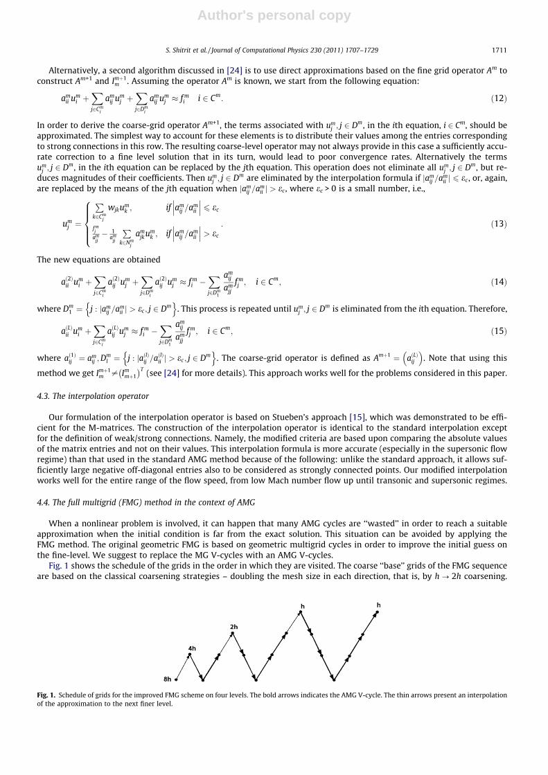
When a nonlinear problem is involved, it can happen that many AMG cycles are ‘‘wasted’’ in order to reach a suitableapproximation when the initial condition is far from the exact solution. This situation can be avoided by applying theFMG method. The original geometric FMG is based on geometric multigrid cycles in order to improve the initial guess onthe fine-level. We suggest to replace the MG V-cycles with an AMG V-cycles.

Fig. 1 shows the schedule of the grids in the order in which they are visited. The coarse ‘‘base’’ grids of the FMG sequenceare based on the classical coarsening strategies – doubling the mesh size in each direction, that is, by h ? 2h coarsening.

Fig. 1. Schedule of grids for the improved FMG scheme on four levels. The bold arrows indicates the AMG V-cycle. The thin arrows present an interpolationof the approximation to the next finer level.



Practically, we solve the problem first on a coarse-grid and then interpolate the solution to the finer level. The interpolatedsolution serves as an initial approximation for the AMG cycle on the finer level. Formally, such an FMG algorithm, based onfour levels, can be described as follows:

1. Initialize I2hh f h ! f 2h; I4h

2hf 2h ! f 4h; . . .

2. Solve the problem on coarsest grid A8hv8h = f8h.3. I4h

8hv8h ! v4h.4. V4h

AMGðv4h; f 4hÞ ! v4h; m0 times.5. I2h

4hv4h ! v2h.6. V2h

AMGðv2h; f 2hÞ ! v2h; m0 times.7. Ih

2hv2h ! vh.8. Vh

AMGðvh; f hÞ ! vh; m0 times.

Instead of transferring the fh to the coarse-level by restriction, the original right hand side f is used for the coarsest level.The cycling parameter m0 sets the number of AMG V-cycles done at each level. Practical experience has shown that m0 de-pends on the problem. Usually for elliptic problems m0 = 1 is sufficient to produce good initial guess for the fine-level.

It is important to mention that this simple FMG algorithm seems still far from being optimal. However, it already appearsto be very instrumental in solving nonlinear problems. We believe there is still much room for optimization, albeit, the re-sults indicate that the algorithm is very efficient even as is.

5. Applications and performance

Several two dimensional flow calculations have been performed to test the performance of the algebraic multigrid meth-od implemented within the body-fitted structured grid and finite volume context. The tests cases were chosen to addresstwo major requirements: First, the flow model problem has to agree the potential flow limitations. Second, it should allowto examine the capability of the code to deal with irregular structured grids together with an equation that becomes extre-mely anisotropic near the sonic case and changes type to hyperbolic in the supersonic flow regime. Two dimensional solu-tions will be given for the following problems: transonic diffuser, rocket chamber, NACA-0012 airfoil, and nonsymmetricNACA-2822 airfoil.

The problems were tested in subsonic and transonic flow regimes in different resolutions. All computational data in thesubsonic flow regime is two order accurate in space and the supersonic region is first order accurate. We consider severalmeasures of the effectiveness of the algorithm. Our focus is on solving the FPE in each case to a high accuracy, namely byreducing the residual by at least ten orders of magnitude. Another relevant measure is the asymptotic convergence factorof the resulting cycle. A lower factor requires fewer iterations in the solution phase. For each V-cycle the columns denotedby Cf reports the convergence factor. In the row denoted by CX, the grid complexity is reported, and the operator complexityis reported as CL. The following default settings were used throughout the calculations, unless explicitly stated otherwise:The second pass process [22] was applied only on the fine-level in order to satisfy the interpolation requirements. Strongconnectivity is defined by a fixed threshold e = 0.25. The dynamic threshold was applied only where the fixed threshold fails.A symmetric Gauss–Seidel, two pre and two post smoothing steps being the default.

5.1. Transonic diffuser

Converging–diverging diffuser is an important and basic component associated with propulsion and the high speed flowof gases. This application often places high demands on CFD codes. For example, one purpose of the diffuser is to deceleratethe flow ahead of the engine. Another purpose of the diffuser is to connect the inlet with the engine. In many cases, the inletand engine axes are offset, and the diffuser must turn the flow [25]. In this exercise, both subsonic and transonic flowthrough a converging–diverging diffuser are investigated. Mach number variation and shock formation may be examined.This flow problem can be found practically in any gas dynamics textbook, for example [26,25].

5.1.1. Problem definition and boundary conditionThe diffuser has a rectangular section. It has a flat bottom wall and a converging–diverging channel with a maximum

divergence angle of 10� at the top wall. The ratio of the inlet area to the throat area is AinAthroat

¼ 1:4114 and the ratio of the exitarea and the throat area is Aout

Athroat¼ 1:5. This problem was solved on grids with three different levels of resolutions in order to

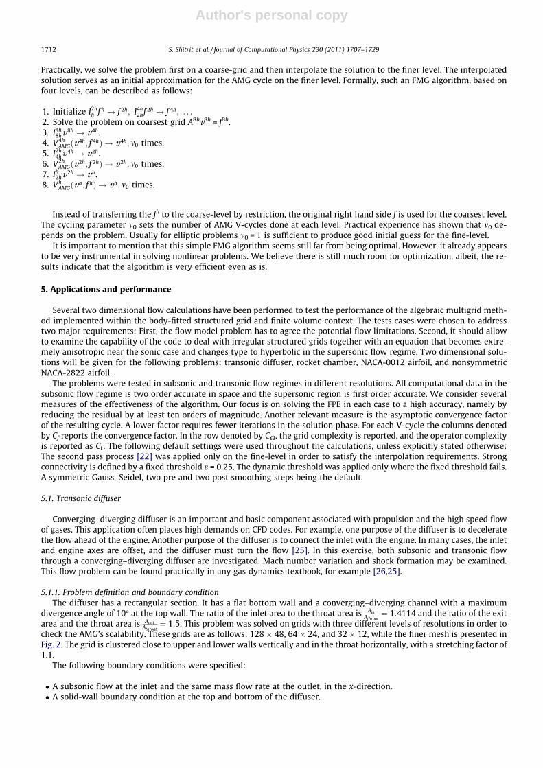
check the AMG’s scalability. These grids are as follows: 128 � 48, 64 � 24, and 32 � 12, while the finer mesh is presented inFig. 2. The grid is clustered close to upper and lower walls vertically and in the throat horizontally, with a stretching factor of1.1.

The following boundary conditions were specified:

� A subsonic flow at the inlet and the same mass flow rate at the outlet, in the x-direction.� A solid-wall boundary condition at the top and bottom of the diffuser.



5.1.2. Qualitative resultsFig. 3(a) shows the flow through the diffuser when it is completely subsonic. The flow accelerates out of the chamber

through the converging section, reaching its maximum speed at the throat. The flow then decelerates through the divergingsection. Fig. 3(d) presents the case where the Mach number at the inlet is increased to M1 = 0.46. The flow at the throatreaches the sonic speed (shocked throat). Unlike the subsonic flow, the supersonic flow accelerates as the cross-section areais increased. The region of the supersonic acceleration is terminated by a normal shock wave, as can be seen in Fig. 3(d).

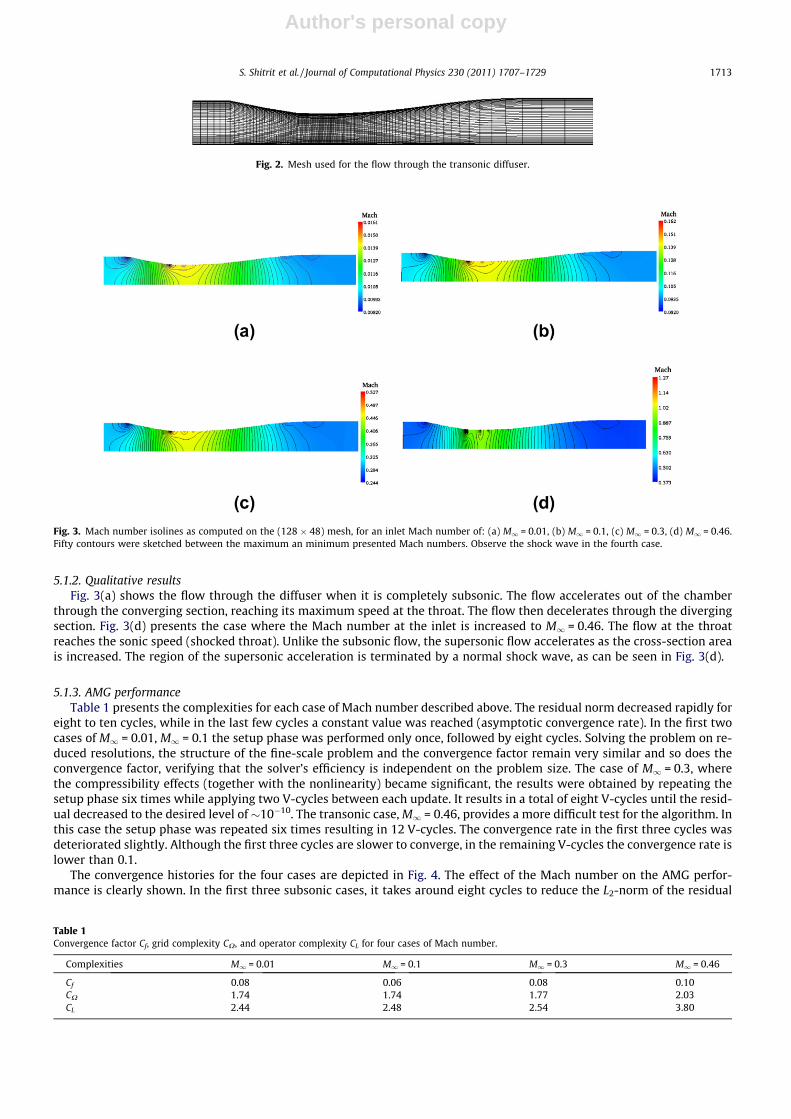
5.1.3. AMG performanceTable 1 presents the complexities for each case of Mach number described above. The residual norm decreased rapidly for

eight to ten cycles, while in the last few cycles a constant value was reached (asymptotic convergence rate). In the first twocases of M1 = 0.01, M1 = 0.1 the setup phase was performed only once, followed by eight cycles. Solving the problem on re-duced resolutions, the structure of the fine-scale problem and the convergence factor remain very similar and so does theconvergence factor, verifying that the solver’s efficiency is independent on the problem size. The case of M1 = 0.3, wherethe compressibility effects (together with the nonlinearity) became significant, the results were obtained by repeating thesetup phase six times while applying two V-cycles between each update. It results in a total of eight V-cycles until the resid-ual decreased to the desired level of �10�10. The transonic case, M1 = 0.46, provides a more difficult test for the algorithm. Inthis case the setup phase was repeated six times resulting in 12 V-cycles. The convergence rate in the first three cycles wasdeteriorated slightly. Although the first three cycles are slower to converge, in the remaining V-cycles the convergence rate islower than 0.1.

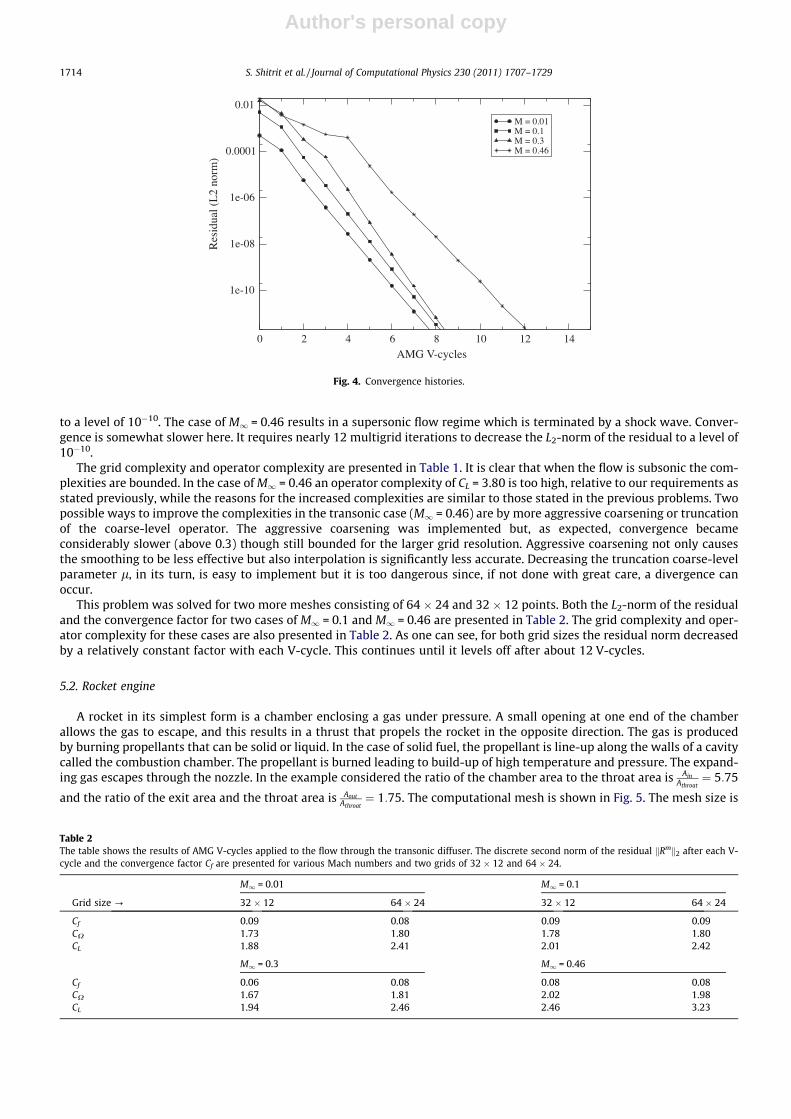
The convergence histories for the four cases are depicted in Fig. 4. The effect of the Mach number on the AMG perfor-mance is clearly shown. In the first three subsonic cases, it takes around eight cycles to reduce the L2-norm of the residual

Fig. 3. Mach number isolines as computed on the (128 � 48) mesh, for an inlet Mach number of: (a) M1 = 0.01, (b) M1 = 0.1, (c) M1 = 0.3, (d) M1 = 0.46.Fifty contours were sketched between the maximum an minimum presented Mach numbers. Observe the shock wave in the fourth case.

Fig. 2. Mesh used for the flow through the transonic diffuser.

Table 1Convergence factor Cf, grid complexity CX, and operator complexity CL for four cases of Mach number.

Complexities M1 = 0.01 M1 = 0.1 M1 = 0.3 M1 = 0.46

Cf 0.08 0.06 0.08 0.10CX 1.74 1.74 1.77 2.03CL 2.44 2.48 2.54 3.80



to a level of 10�10. The case of M1 = 0.46 results in a supersonic flow regime which is terminated by a shock wave. Conver-gence is somewhat slower here. It requires nearly 12 multigrid iterations to decrease the L2-norm of the residual to a level of10�10.

The grid complexity and operator complexity are presented in Table 1. It is clear that when the flow is subsonic the com-plexities are bounded. In the case of M1 = 0.46 an operator complexity of CL = 3.80 is too high, relative to our requirements asstated previously, while the reasons for the increased complexities are similar to those stated in the previous problems. Twopossible ways to improve the complexities in the transonic case (M1 = 0.46) are by more aggressive coarsening or truncationof the coarse-level operator. The aggressive coarsening was implemented but, as expected, convergence becameconsiderably slower (above 0.3) though still bounded for the larger grid resolution. Aggressive coarsening not only causesthe smoothing to be less effective but also interpolation is significantly less accurate. Decreasing the truncation coarse-levelparameter l, in its turn, is easy to implement but it is too dangerous since, if not done with great care, a divergence canoccur.

This problem was solved for two more meshes consisting of 64 � 24 and 32 � 12 points. Both the L2-norm of the residualand the convergence factor for two cases of M1 = 0.1 and M1 = 0.46 are presented in Table 2. The grid complexity and oper-ator complexity for these cases are also presented in Table 2. As one can see, for both grid sizes the residual norm decreasedby a relatively constant factor with each V-cycle. This continues until it levels off after about 12 V-cycles.

5.2. Rocket engine

A rocket in its simplest form is a chamber enclosing a gas under pressure. A small opening at one end of the chamberallows the gas to escape, and this results in a thrust that propels the rocket in the opposite direction. The gas is producedby burning propellants that can be solid or liquid. In the case of solid fuel, the propellant is line-up along the walls of a cavitycalled the combustion chamber. The propellant is burned leading to build-up of high temperature and pressure. The expand-ing gas escapes through the nozzle. In the example considered the ratio of the chamber area to the throat area is Ain

Athroat¼ 5:75

and the ratio of the exit area and the throat area is AoutAthroat

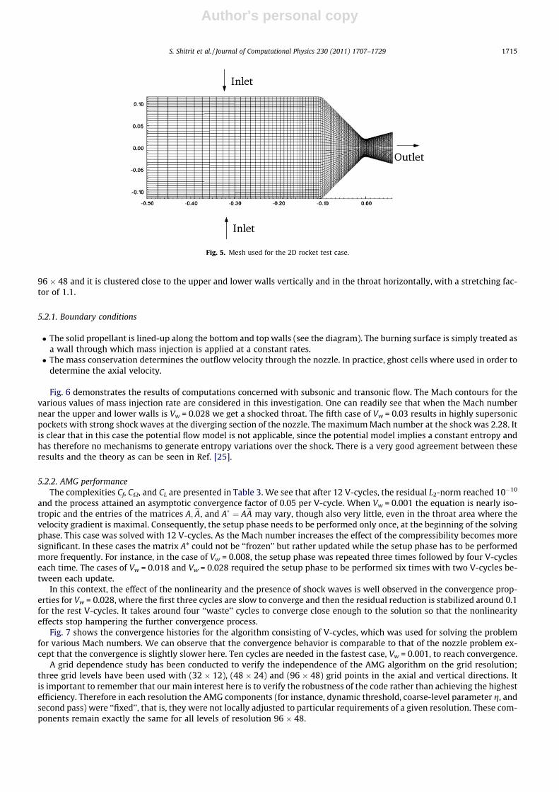
¼ 1:75. The computational mesh is shown in Fig. 5. The mesh size is

0 2 4 6 8 10 12 14

AMG V-cycles

1e-10

1e-08

1e-06

0.0001

0.01

Res

idua

l (L

2 no

rm)

M = 0.01M = 0.1M = 0.3M = 0.46

Fig. 4. Convergence histories.

Table 2The table shows the results of AMG V-cycles applied to the flow through the transonic diffuser. The discrete second norm of the residual kRmk2 after each V-cycle and the convergence factor Cf are presented for various Mach numbers and two grids of 32 � 12 and 64 � 24.

M1 = 0.01 M1 = 0.1

Grid size ? 32 � 12 64 � 24 32 � 12 64 � 24

Cf 0.09 0.08 0.09 0.09CX 1.73 1.80 1.78 1.80CL 1.88 2.41 2.01 2.42

M1 = 0.3 M1 = 0.46

Cf 0.06 0.08 0.08 0.08CX 1.67 1.81 2.02 1.98CL 1.94 2.46 2.46 3.23



96 � 48 and it is clustered close to the upper and lower walls vertically and in the throat horizontally, with a stretching fac-tor of 1.1.

5.2.1. Boundary conditions

� The solid propellant is lined-up along the bottom and top walls (see the diagram). The burning surface is simply treated asa wall through which mass injection is applied at a constant rates.� The mass conservation determines the outflow velocity through the nozzle. In practice, ghost cells where used in order to

determine the axial velocity.

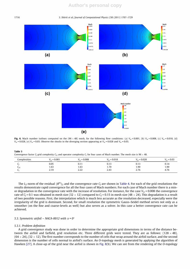
Fig. 6 demonstrates the results of computations concerned with subsonic and transonic flow. The Mach contours for thevarious values of mass injection rate are considered in this investigation. One can readily see that when the Mach numbernear the upper and lower walls is Vw = 0.028 we get a shocked throat. The fifth case of Vw = 0.03 results in highly supersonicpockets with strong shock waves at the diverging section of the nozzle. The maximum Mach number at the shock was 2.28. Itis clear that in this case the potential flow model is not applicable, since the potential model implies a constant entropy andhas therefore no mechanisms to generate entropy variations over the shock. There is a very good agreement between theseresults and the theory as can be seen in Ref. [25].

5.2.2. AMG performanceThe complexities Cf, CX, and CL are presented in Table 3. We see that after 12 V-cycles, the residual L2-norm reached 10�10

and the process attained an asymptotic convergence factor of 0.05 per V-cycle. When Vw = 0.001 the equation is nearly iso-tropic and the entries of the matrices A; eA, and A� ¼ AeA may vary, though also very little, even in the throat area where thevelocity gradient is maximal. Consequently, the setup phase needs to be performed only once, at the beginning of the solvingphase. This case was solved with 12 V-cycles. As the Mach number increases the effect of the compressibility becomes moresignificant. In these cases the matrix A* could not be ‘‘frozen’’ but rather updated while the setup phase has to be performedmore frequently. For instance, in the case of Vw = 0.008, the setup phase was repeated three times followed by four V-cycleseach time. The cases of Vw = 0.018 and Vw = 0.028 required the setup phase to be performed six times with two V-cycles be-tween each update.

In this context, the effect of the nonlinearity and the presence of shock waves is well observed in the convergence prop-erties for Vw = 0.028, where the first three cycles are slow to converge and then the residual reduction is stabilized around 0.1for the rest V-cycles. It takes around four ‘‘waste’’ cycles to converge close enough to the solution so that the nonlinearityeffects stop hampering the further convergence process.

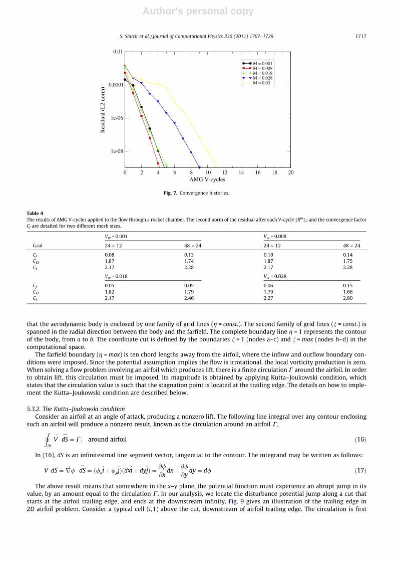
Fig. 7 shows the convergence histories for the algorithm consisting of V-cycles, which was used for solving the problemfor various Mach numbers. We can observe that the convergence behavior is comparable to that of the nozzle problem ex-cept that the convergence is slightly slower here. Ten cycles are needed in the fastest case, Vw = 0.001, to reach convergence.

A grid dependence study has been conducted to verify the independence of the AMG algorithm on the grid resolution;three grid levels have been used with (32 � 12), (48 � 24) and (96 � 48) grid points in the axial and vertical directions. Itis important to remember that our main interest here is to verify the robustness of the code rather than achieving the highestefficiency. Therefore in each resolution the AMG components (for instance, dynamic threshold, coarse-level parameter g, andsecond pass) were ‘‘fixed’’, that is, they were not locally adjusted to particular requirements of a given resolution. These com-ponents remain exactly the same for all levels of resolution 96 � 48.

Fig. 5. Mesh used for the 2D rocket test case.



The L2-norm of the residual kRmk2 and the convergence rate Cf are shown in Table 4. For each of the grid resolutions theresults demonstrate rapid convergence for all the four cases of Mach numbers. For each case of Mach number there is a min-or degradation in the convergence rate with the increase of resolution. For instance, for the case Vw = 0.008 the convergencerate of Cf = 0.1 was obtained in mesh size (32 � 12) compared to Cf = 0.15 in mesh size (48 � 24). This degradation is a resultof two possible reasons. First, the interpolation which is much less accurate as the resolution decreased, especially were theirregularity of the grid is dominant. Second, for small resolution the symmetric Gauss–Seidel method serves not only as asmoother (on the fine and coarse-levels as well) but also serves as a solver. In this case a better convergence rate can beachieved.

5.3. Symmetric airfoil – NACA-0012 with a = 0�

5.3.1. Problem definitionA grid convergence study was done in order to determine the appropriate grid dimensions in terms of the distance be-

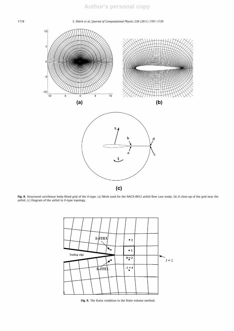
tween the airfoil and farfield, grid resolution etc. Three different grids were tested. They are as follows: (128 � 48),(64 � 24), (32 � 12). The first number corresponds to the number of cells that wrap around the airfoil surface, and the seconddimension is the number of cells normal to airfoil’s surface. An O-topology mesh is generated by applying the algorithm ofHawken [27]. A close-up of the grid near the airfoil is shown in Fig. 8(b). We can see from the rendering of the O-topology

Fig. 6. Mach number isolines computed on the (96 � 48) mesh, for the following flow conditions: (a) Vw = 0.001, (b) Vw = 0.008, (c) Vw = 0.018, (d)Vw = 0.028, (e) Vw = 0.03. Observe the shocks in the diverging section appearing at Vw = 0.028 and Vw = 0.03.

Table 3Convergence factor Cf grid complexity CX and operator complexity CL for four cases of Mach number. The mesh size is 96 � 48.

Complexities Vw = 0.001 Vw = 0.008 Vw = 0.018 Vw = 0.028 Vw = 0.03

Cf 0.05 0.11 0.13 0.13 0.14CX 1.63 1.63 1.70 1.90 1.90CL 2.19 2.22 2.43 2.76 4.76



that the aerodynamic body is enclosed by one family of grid lines (g = const.). The second family of grid lines (n = const.) isspanned in the radial direction between the body and the farfield. The complete boundary line g = 1 represents the contourof the body, from a to b. The coordinate cut is defined by the boundaries n = 1 (nodes a–c) and n = max (nodes b–d) in thecomputational space.

The farfield boundary (g = max) is ten chord lengths away from the airfoil, where the inflow and outflow boundary con-ditions were imposed. Since the potential assumption implies the flow is irrotational, the local vorticity production is zero.When solving a flow problem involving an airfoil which produces lift, there is a finite circulation C around the airfoil. In orderto obtain lift, this circulation must be imposed. Its magnitude is obtained by applying Kutta–Joukowski condition, whichstates that the circulation value is such that the stagnation point is located at the trailing edge. The details on how to imple-ment the Kutta–Joukowski condition are described below.

5.3.2. The Kutta–Joukowski conditionConsider an airfoil at an angle of attack, producing a nonzero lift. The following line integral over any contour enclosing

such an airfoil will produce a nonzero result, known as the circulation around an airfoil C,I@s

V!� dS!¼ C: around airfoil ð16Þ

In (16), dS is an infinitesimal line segment vector, tangential to the contour. The integrand may be written as follows:

V!�dS ¼ ~r/ � dS

!¼ ð/xiþ /yjÞðdxiþ dyjÞ ¼ @/

@xdxþ @/

@ydy ¼ d/: ð17Þ

The above result means that somewhere in the x–y plane, the potential function must experience an abrupt jump in itsvalue, by an amount equal to the circulation C. In our analysis, we locate the disturbance potential jump along a cut thatstarts at the airfoil trailing edge, and ends at the downstream infinity. Fig. 9 gives an illustration of the trailing edge in2D airfoil problem. Consider a typical cell (i,1) above the cut, downstream of airfoil trailing edge. The circulation is first

0 2 4 6 8 10 12 14 16 18 20AMG V-cycles

1e-08

1e-06

0.0001

0.01

Res

idua

l (L

2 no

rm)

M = 0.001M = 0.008M = 0.018M = 0.028M = 0.03


Table 4The results of AMG V-cycles applied to the flow through a rocket chamber. The second norm of the residual after each V-cycle kRmk2 and the convergence factorCf are detailed for two different mesh sizes.

Vw = 0.001 Vw = 0.008

Grid 24 � 12 48 � 24 24 � 12 48 � 24

Cf 0.08 0.13 0.10 0.14CX 1.87 1.74 1.87 1.75CL 2.17 2.28 2.17 2.28

Vw = 0.018 Vw = 0.028

Cf 0.05 0.05 0.06 0.15CX 1.82 1.79 1.79 1.66CL 2.17 2.46 2.27 2.80



Fig. 8. Structured curvilinear body-fitted grid of the O-type. (a) Mesh used for the NACA-0012 airfoil flow case study. (b) A close-up of the grid near theairfoil. (c) Diagram of the airfoil in O-type topology.

Fig. 9. The Kutta condition in the finite volume method.



computed as, C = /TE,top � /TE, bottom, where /TE,top and /TE,bottom are the potential values at the trailing edges for the top andbottom points, respectively. In Fig. 9, the values of the potential /TE,top and /TE,bottom are known, where the subscripts TE, topand TE, bottom correspond to the trailing edge upper and lower i coordinates, respectively. Since these values are defined atthe cell’s center, and are not known at the trailing edge, an extrapolation is needed. Once the circulation value is calculated,the next step is to apply the potential jump. All the cells above and below the cut which is drawn from the airfoil surface tothe farfield boundary, will have their value of potential modified to satisfy the proper jump condition. It is done as follows:

/i;0 ¼ /i;jmax þ C;

/i;�1 ¼ /i;jmax�1 þ C;

/i;jmaxþ1 ¼ /i;1 � C;

/i;jmaxþ2 ¼ /i;2 � C:

ð18Þ

5.3.3. Boundary conditionsFor the airfoil surface, a solid wall boundary condition is applied (no penetration), qV

!�n ¼ q @/

@n ¼ 0. There are two ways inwhich the farfield boundary condition are imposed. The first method, which is chosen to be implemented in this researchwork, is by using a Neumann boundary condition at the farfield. The flow field is assumed to be known at the farfieldand is taken to be free-stream condition. Practically, it is implemented by projecting the free-steam velocity V1 normalto cell’s face.

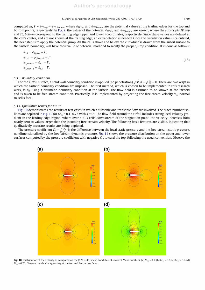
5.3.4. Qualitative results for a = 0�Fig. 10 demonstrates the results of test cases in which a subsonic and transonic flow are involved. The Mach number iso-

lines are depicted in Fig. 10 for M1 = 0.1–0.76 with a = 0�. The flow-field around the airfoil includes strong local velocity gra-dient in the leading edge region, where over a 2–3 cells downstream of the stagnation point, the velocity increases fromnearly zero to values larger than the incoming free-stream velocity. The following basic features are visible, indicating thatqualitatively accurate results are being depicted.

The pressure coefficient Cp ¼ p�p112q1u2

1is the difference between the local static pressure and the free-stream static pressure,

nondimensionalized by the free-stream dynamic pressure. Fig. 11 shows the pressure distribution on the upper and lowersurfaces computed by the pressure coefficient with negative Cp, toward the top, following the usual convention. Observe the

Fig. 10. Distribution of the velocity as computed on the (128 � 48) mesh, for different incident Mash numbers. (a) M1 = 0.1, (b) M1 = 0.3, (c) M1 = 0.5, (d)M1 = 0.76. Observe the shocks appearing at the top and bottom surfaces.



sharp decrease in Cp across the shock wave. The M1 = 0.1 and M1 = 0.3 cases have a slight difference in both the convergenceand Cp solution. The flow is nearly incompressible at these speeds, giving very little differences in the results. At M1 = 0.5 thecompressibility of the flow become more significant, and at M1 = 0.76 the compressibility effects are very evident.

5.3.5. AMG performanceIn the subsonic cases, M1 6 0.5 the coarse-levels were obtained while applying a fixed threshold (e = 0.25). It was suffi-

cient to apply the second-pass process in the first coarsening step and maintain standard coarsening for all subsequent lev-els. In the transonic case, M1 = 0.76 a dynamic threshold produced much better results (in terms of convergence properties)but on the expense of somewhat higher memory requirements.

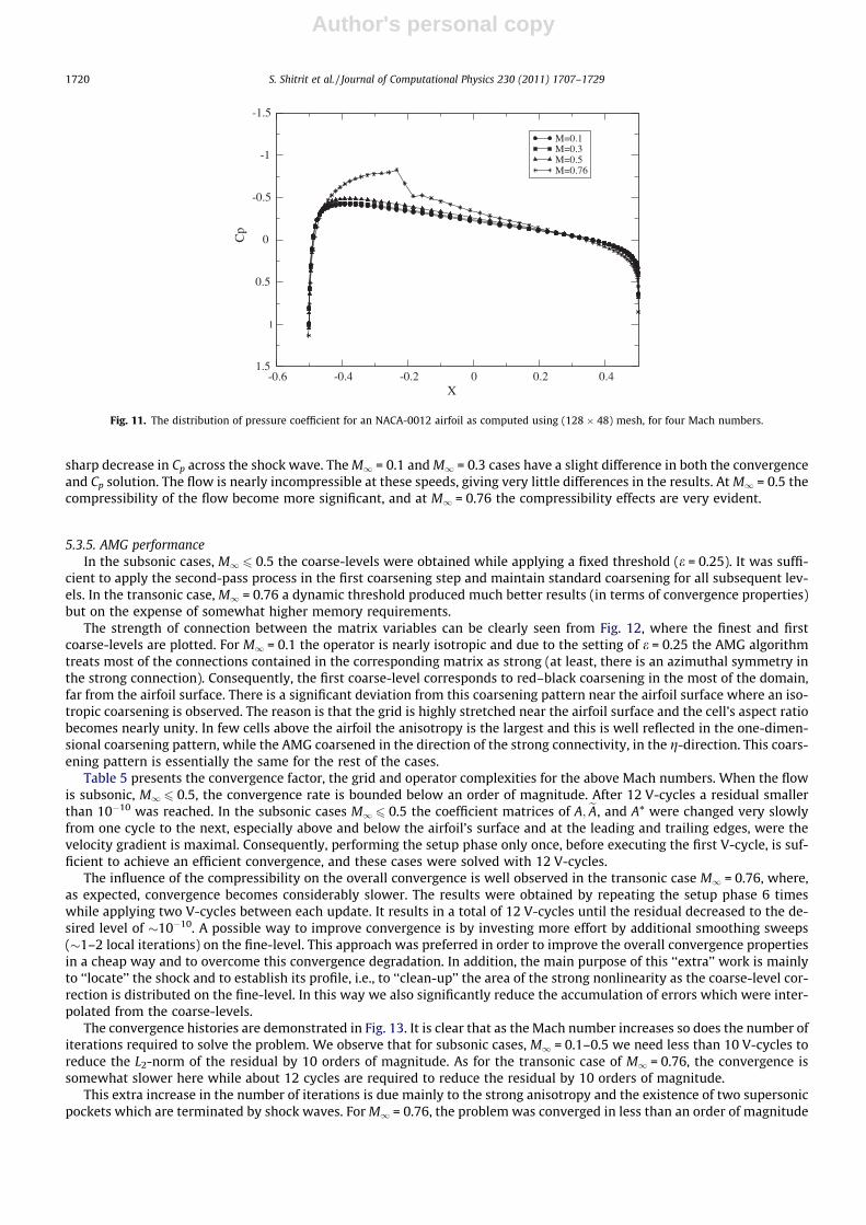
The strength of connection between the matrix variables can be clearly seen from Fig. 12, where the finest and firstcoarse-levels are plotted. For M1 = 0.1 the operator is nearly isotropic and due to the setting of e = 0.25 the AMG algorithmtreats most of the connections contained in the corresponding matrix as strong (at least, there is an azimuthal symmetry inthe strong connection). Consequently, the first coarse-level corresponds to red–black coarsening in the most of the domain,far from the airfoil surface. There is a significant deviation from this coarsening pattern near the airfoil surface where an iso-tropic coarsening is observed. The reason is that the grid is highly stretched near the airfoil surface and the cell’s aspect ratiobecomes nearly unity. In few cells above the airfoil the anisotropy is the largest and this is well reflected in the one-dimen-sional coarsening pattern, while the AMG coarsened in the direction of the strong connectivity, in the g-direction. This coars-ening pattern is essentially the same for the rest of the cases.

Table 5 presents the convergence factor, the grid and operator complexities for the above Mach numbers. When the flowis subsonic, M1 6 0.5, the convergence rate is bounded below an order of magnitude. After 12 V-cycles a residual smallerthan 10�10 was reached. In the subsonic cases M1 6 0.5 the coefficient matrices of A; eA, and A* were changed very slowlyfrom one cycle to the next, especially above and below the airfoil’s surface and at the leading and trailing edges, were thevelocity gradient is maximal. Consequently, performing the setup phase only once, before executing the first V-cycle, is suf-ficient to achieve an efficient convergence, and these cases were solved with 12 V-cycles.

The influence of the compressibility on the overall convergence is well observed in the transonic case M1 = 0.76, where,as expected, convergence becomes considerably slower. The results were obtained by repeating the setup phase 6 timeswhile applying two V-cycles between each update. It results in a total of 12 V-cycles until the residual decreased to the de-sired level of �10�10. A possible way to improve convergence is by investing more effort by additional smoothing sweeps(�1–2 local iterations) on the fine-level. This approach was preferred in order to improve the overall convergence propertiesin a cheap way and to overcome this convergence degradation. In addition, the main purpose of this ‘‘extra’’ work is mainlyto ‘‘locate’’ the shock and to establish its profile, i.e., to ‘‘clean-up’’ the area of the strong nonlinearity as the coarse-level cor-rection is distributed on the fine-level. In this way we also significantly reduce the accumulation of errors which were inter-polated from the coarse-levels.

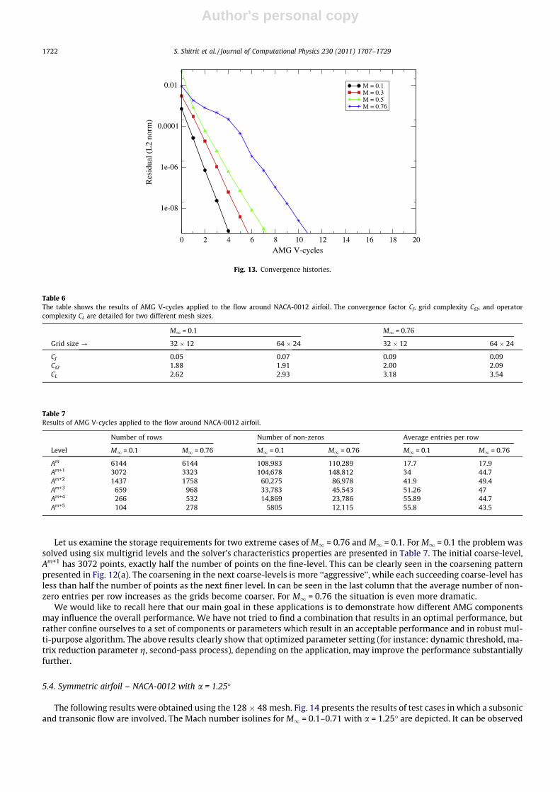
The convergence histories are demonstrated in Fig. 13. It is clear that as the Mach number increases so does the number ofiterations required to solve the problem. We observe that for subsonic cases, M1 = 0.1–0.5 we need less than 10 V-cycles toreduce the L2-norm of the residual by 10 orders of magnitude. As for the transonic case of M1 = 0.76, the convergence issomewhat slower here while about 12 cycles are required to reduce the residual by 10 orders of magnitude.

This extra increase in the number of iterations is due mainly to the strong anisotropy and the existence of two supersonicpockets which are terminated by shock waves. For M1 = 0.76, the problem was converged in less than an order of magnitude

-0.6 -0.4 -0.2 0 0.2 0.4X

-1.5

-1

-0.5

0

0.5

1

1.5

Cp

M=0.1M=0.3M=0.5M=0.76

Fig. 11. The distribution of pressure coefficient for an NACA-0012 airfoil as computed using (128 � 48) mesh, for four Mach numbers.



per V-cycle, and a much higher operator complexity of CX = 3.89 was obtained. This behavior is typical of the more generalproblems which are characterized by a strong anisotropy and nonlinearity. Combinations of AMG components that producethe best convergence rates are also those with the higher costs in terms of grid and operator complexity. Parameter selectionis largely the art of finding a compromise between performance and cost.

This problem was solved for two more grid sizes of 64 � 24 and 32 � 12. The complexities are presented in Table 6. This isa case where applying AMG convergence acceleration is a very attractive possibility since it is precisely a situation for whichconstructing an efficient geometric multigrid approach would become extremely cumbersome. We observe that for subsonicflow, the AMG exhibits the same type of convergence that was observed in the previous problems. As the Mach number in-creases the convergence deteriorates but, we find the solver to still be very efficient for this problem, despite of the strongnonlinearity and the anisotropy of the problem. The storage requirement is higher than that for the subsonic case (isotropiccase), the reason being that AMG performs one-dimensional coarsening in the azimuthal direction at the farfield since thestrong connection in the n-direction (azimuthal direction) arises from a large grid spacing in g-direction. In this respect, thecomplexities deteriorate significantly.

Fig. 12. The finest and first coarse-level for mesh size (128 � 48). The red color corresponds to the a C-point and the blue color corresponds to an F-point. (a)M1 = 0.1, (b) M1 = 0.76. The pictures on the right are magnified views of the airfoil’s region. (For interpretation of the references to colour in this figurelegend, the reader is referred to the web version of this article.)

Table 5Convergence factor Cf, grid complexity CX and operator complexity CL for four cases of Mach number.


Cf 0.04 0.05 0.11 0.18CX 1.90 1.93 2.13 1.92CL 3.01 2.95 3.87 3.89



Let us examine the storage requirements for two extreme cases of M1 = 0.76 and M1 = 0.1. For M1 = 0.1 the problem wassolved using six multigrid levels and the solver’s characteristics properties are presented in Table 7. The initial coarse-level,Am+1 has 3072 points, exactly half the number of points on the fine-level. This can be clearly seen in the coarsening patternpresented in Fig. 12(a). The coarsening in the next coarse-levels is more ‘‘aggressive’’, while each succeeding coarse-level hasless than half the number of points as the next finer level. In can be seen in the last column that the average number of non-zero entries per row increases as the grids become coarser. For M1 = 0.76 the situation is even more dramatic.

We would like to recall here that our main goal in these applications is to demonstrate how different AMG componentsmay influence the overall performance. We have not tried to find a combination that results in an optimal performance, butrather confine ourselves to a set of components or parameters which result in an acceptable performance and in robust mul-ti-purpose algorithm. The above results clearly show that optimized parameter setting (for instance: dynamic threshold, ma-trix reduction parameter g, second-pass process), depending on the application, may improve the performance substantiallyfurther.

5.4. Symmetric airfoil – NACA-0012 with a = 1.25�

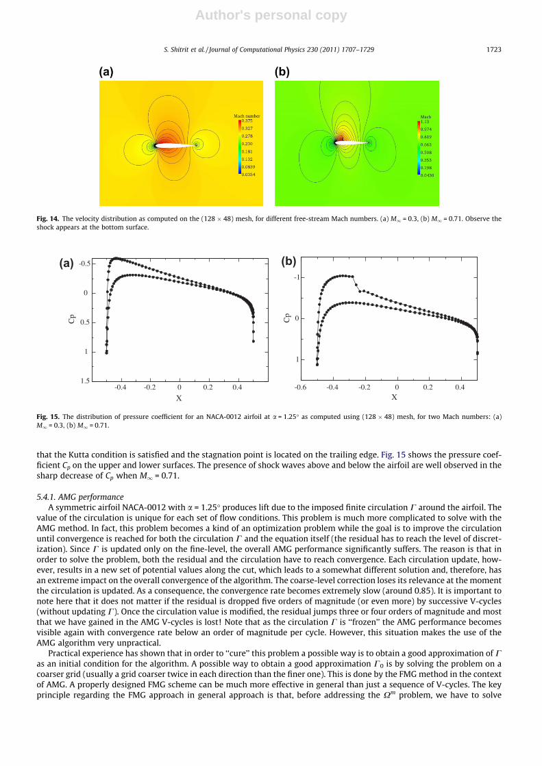
The following results were obtained using the 128 � 48 mesh. Fig. 14 presents the results of test cases in which a subsonicand transonic flow are involved. The Mach number isolines for M1 = 0.1–0.71 with a = 1.25� are depicted. It can be observed

0 2 4 6 8 10 12 14 16 18 20AMG V-cycles

1e-08

1e-06

0.0001

0.01

Res

idua

l (L

2 no

rm)

M = 0.1M = 0.3M = 0.5M = 0.76


Table 6The table shows the results of AMG V-cycles applied to the flow around NACA-0012 airfoil. The convergence factor Cf, grid complexity CX, and operatorcomplexity CL are detailed for two different mesh sizes.

M1 = 0.1 M1 = 0.76

Grid size ? 32 � 12 64 � 24 32 � 12 64 � 24

Cf 0.05 0.07 0.09 0.09CX 1.88 1.91 2.00 2.09CL 2.62 2.93 3.18 3.54

Table 7Results of AMG V-cycles applied to the flow around NACA-0012 airfoil.

Number of rows Number of non-zeros Average entries per row

Level M1 = 0.1 M1 = 0.76 M1 = 0.1 M1 = 0.76 M1 = 0.1 M1 = 0.76

Am 6144 6144 108,983 110,289 17.7 17.9Am+1 3072 3323 104,678 148,812 34 44.7Am+2 1437 1758 60,275 86,978 41.9 49.4Am+3 659 968 33,783 45,543 51.26 47Am+4 266 532 14,869 23,786 55.89 44.7Am+5 104 278 5805 12,115 55.8 43.5



that the Kutta condition is satisfied and the stagnation point is located on the trailing edge. Fig. 15 shows the pressure coef-ficient Cp on the upper and lower surfaces. The presence of shock waves above and below the airfoil are well observed in thesharp decrease of Cp when M1 = 0.71.

5.4.1. AMG performanceA symmetric airfoil NACA-0012 with a = 1.25� produces lift due to the imposed finite circulation C around the airfoil. The

value of the circulation is unique for each set of flow conditions. This problem is much more complicated to solve with theAMG method. In fact, this problem becomes a kind of an optimization problem while the goal is to improve the circulationuntil convergence is reached for both the circulation C and the equation itself (the residual has to reach the level of discret-ization). Since C is updated only on the fine-level, the overall AMG performance significantly suffers. The reason is that inorder to solve the problem, both the residual and the circulation have to reach convergence. Each circulation update, how-ever, results in a new set of potential values along the cut, which leads to a somewhat different solution and, therefore, hasan extreme impact on the overall convergence of the algorithm. The coarse-level correction loses its relevance at the momentthe circulation is updated. As a consequence, the convergence rate becomes extremely slow (around 0.85). It is important tonote here that it does not matter if the residual is dropped five orders of magnitude (or even more) by successive V-cycles(without updating C). Once the circulation value is modified, the residual jumps three or four orders of magnitude and mostthat we have gained in the AMG V-cycles is lost! Note that as the circulation C is ‘‘frozen’’ the AMG performance becomesvisible again with convergence rate below an order of magnitude per cycle. However, this situation makes the use of theAMG algorithm very unpractical.

Practical experience has shown that in order to ‘‘cure’’ this problem a possible way is to obtain a good approximation of Cas an initial condition for the algorithm. A possible way to obtain a good approximation C0 is by solving the problem on acoarser grid (usually a grid coarser twice in each direction than the finer one). This is done by the FMG method in the contextof AMG. A properly designed FMG scheme can be much more effective in general than just a sequence of V-cycles. The keyprinciple regarding the FMG approach in general approach is that, before addressing the Xm problem, we have to solve

Fig. 14. The velocity distribution as computed on the (128 � 48) mesh, for different free-stream Mach numbers. (a) M1 = 0.3, (b) M1 = 0.71. Observe theshock appears at the bottom surface.

X X

-0.5

0

0.5

1

1.5

Cp

-0.4 -0.2 0 0.2 0.4 -0.6 -0.4 -0.2 0 0.2 0.4

-1

0

1

Cp

(b)(a)

Fig. 15. The distribution of pressure coefficient for an NACA-0012 airfoil at a = 1.25� as computed using (128 � 48) mesh, for two Mach numbers: (a)M1 = 0.3, (b) M1 = 0.71.



the X2m problem to the level of discretization error. In our case here this also result in a good approximation to the circu-lation value C0 (its value is within �1–3% of the value of C that is obtained on the fine-level Xm) as an initial condition. It isvery important to mention that the convergence rate of these nonlinear iterations (especially in the transonic case where thenonlinearity is significant) depends dramatically on a quality of the initial condition for C. The better the initial guess C0

used on the fine-level, the more effective the AMG V-cycle will be. In our test-case the FMG scheme relies on four levels,while on the coarsest level (16 � 6 grid) the problem was solved to the level of machine zero.

The practical implementation of this problem, relies heavily upon the way the treatment of the circulation value is incor-porated in each V-cycle. The value of the circulation C is updated at the end of each V-cycle, immediately after the correctionfrom the coarse-levels is distributed to the points on the fine-level. A possible way to improve the convergence is to use asimple 2D linear extrapolation of the circulation value. If the circulation value is known in the present and last iterations thenext value can be calculated as follows: an ‘‘over-relaxation’’ parameter 1 6x 6 2 can be added in order to accelerateconvergence:

Cnew ¼ Cnþ1 þxðCnþ1 � CnÞ: ð19Þ

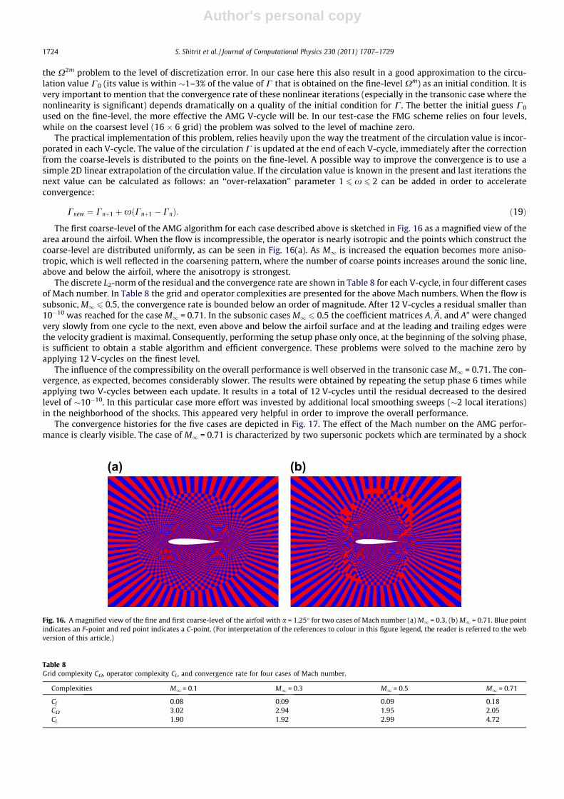
The first coarse-level of the AMG algorithm for each case described above is sketched in Fig. 16 as a magnified view of thearea around the airfoil. When the flow is incompressible, the operator is nearly isotropic and the points which construct thecoarse-level are distributed uniformly, as can be seen in Fig. 16(a). As M1 is increased the equation becomes more aniso-tropic, which is well reflected in the coarsening pattern, where the number of coarse points increases around the sonic line,above and below the airfoil, where the anisotropy is strongest.

The discrete L2-norm of the residual and the convergence rate are shown in Table 8 for each V-cycle, in four different casesof Mach number. In Table 8 the grid and operator complexities are presented for the above Mach numbers. When the flow issubsonic, M1 6 0.5, the convergence rate is bounded below an order of magnitude. After 12 V-cycles a residual smaller than10�10 was reached for the case M1 = 0.71. In the subsonic cases M1 6 0.5 the coefficient matrices A; eA, and A* were changedvery slowly from one cycle to the next, even above and below the airfoil surface and at the leading and trailing edges werethe velocity gradient is maximal. Consequently, performing the setup phase only once, at the beginning of the solving phase,is sufficient to obtain a stable algorithm and efficient convergence. These problems were solved to the machine zero byapplying 12 V-cycles on the finest level.

The influence of the compressibility on the overall performance is well observed in the transonic case M1 = 0.71. The con-vergence, as expected, becomes considerably slower. The results were obtained by repeating the setup phase 6 times whileapplying two V-cycles between each update. It results in a total of 12 V-cycles until the residual decreased to the desiredlevel of �10�10. In this particular case more effort was invested by additional local smoothing sweeps (�2 local iterations)in the neighborhood of the shocks. This appeared very helpful in order to improve the overall performance.

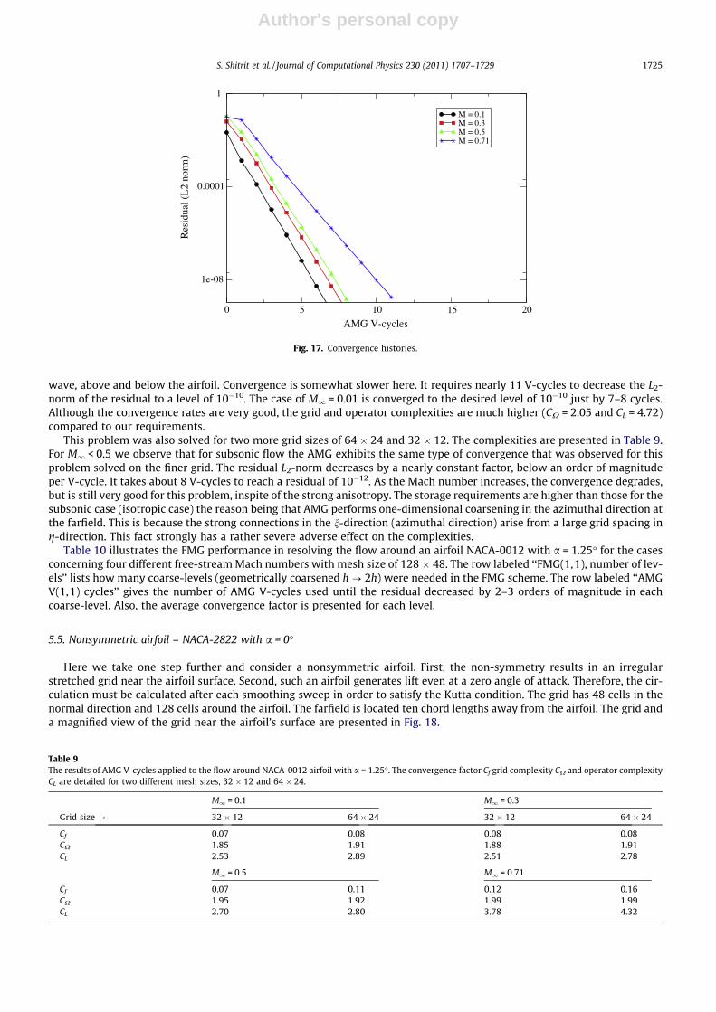
The convergence histories for the five cases are depicted in Fig. 17. The effect of the Mach number on the AMG perfor-mance is clearly visible. The case of M1 = 0.71 is characterized by two supersonic pockets which are terminated by a shock

Fig. 16. A magnified view of the fine and first coarse-level of the airfoil with a = 1.25� for two cases of Mach number (a) M1 = 0.3, (b) M1 = 0.71. Blue pointindicates an F-point and red point indicates a C-point. (For interpretation of the references to colour in this figure legend, the reader is referred to the webversion of this article.)

Table 8Grid complexity CX, operator complexity CL, and convergence rate for four cases of Mach number.


Cf 0.08 0.09 0.09 0.18CX 3.02 2.94 1.95 2.05CL 1.90 1.92 2.99 4.72



wave, above and below the airfoil. Convergence is somewhat slower here. It requires nearly 11 V-cycles to decrease the L2-norm of the residual to a level of 10�10. The case of M1 = 0.01 is converged to the desired level of 10�10 just by 7–8 cycles.Although the convergence rates are very good, the grid and operator complexities are much higher (CX = 2.05 and CL = 4.72)compared to our requirements.

This problem was also solved for two more grid sizes of 64 � 24 and 32 � 12. The complexities are presented in Table 9.For M1 < 0.5 we observe that for subsonic flow the AMG exhibits the same type of convergence that was observed for thisproblem solved on the finer grid. The residual L2-norm decreases by a nearly constant factor, below an order of magnitudeper V-cycle. It takes about 8 V-cycles to reach a residual of 10�12. As the Mach number increases, the convergence degrades,but is still very good for this problem, inspite of the strong anisotropy. The storage requirements are higher than those for thesubsonic case (isotropic case) the reason being that AMG performs one-dimensional coarsening in the azimuthal direction atthe farfield. This is because the strong connections in the n-direction (azimuthal direction) arise from a large grid spacing ing-direction. This fact strongly has a rather severe adverse effect on the complexities.

Table 10 illustrates the FMG performance in resolving the flow around an airfoil NACA-0012 with a = 1.25� for the casesconcerning four different free-stream Mach numbers with mesh size of 128 � 48. The row labeled ‘‘FMG(1,1), number of lev-els’’ lists how many coarse-levels (geometrically coarsened h ? 2h) were needed in the FMG scheme. The row labeled ‘‘AMGV(1,1) cycles’’ gives the number of AMG V-cycles used until the residual decreased by 2–3 orders of magnitude in eachcoarse-level. Also, the average convergence factor is presented for each level.

5.5. Nonsymmetric airfoil – NACA-2822 with a = 0�

Here we take one step further and consider a nonsymmetric airfoil. First, the non-symmetry results in an irregularstretched grid near the airfoil surface. Second, such an airfoil generates lift even at a zero angle of attack. Therefore, the cir-culation must be calculated after each smoothing sweep in order to satisfy the Kutta condition. The grid has 48 cells in thenormal direction and 128 cells around the airfoil. The farfield is located ten chord lengths away from the airfoil. The grid anda magnified view of the grid near the airfoil’s surface are presented in Fig. 18.

0 5 10 15 20

AMG V-cycles

1e-08

0.0001

1

Res

idua

l (L

2 no

rm)

M = 0.1M = 0.3M = 0.5M = 0.71


Table 9The results of AMG V-cycles applied to the flow around NACA-0012 airfoil with a = 1.25�. The convergence factor Cf grid complexity CX and operator complexityCL are detailed for two different mesh sizes, 32 � 12 and 64 � 24.

M1 = 0.1 M1 = 0.3

Grid size ? 32 � 12 64 � 24 32 � 12 64 � 24

Cf 0.07 0.08 0.08 0.08CX 1.85 1.91 1.88 1.91CL 2.53 2.89 2.51 2.78

M1 = 0.5 M1 = 0.71

Cf 0.07 0.11 0.12 0.16CX 1.95 1.92 1.99 1.99CL 2.70 2.80 3.78 4.32



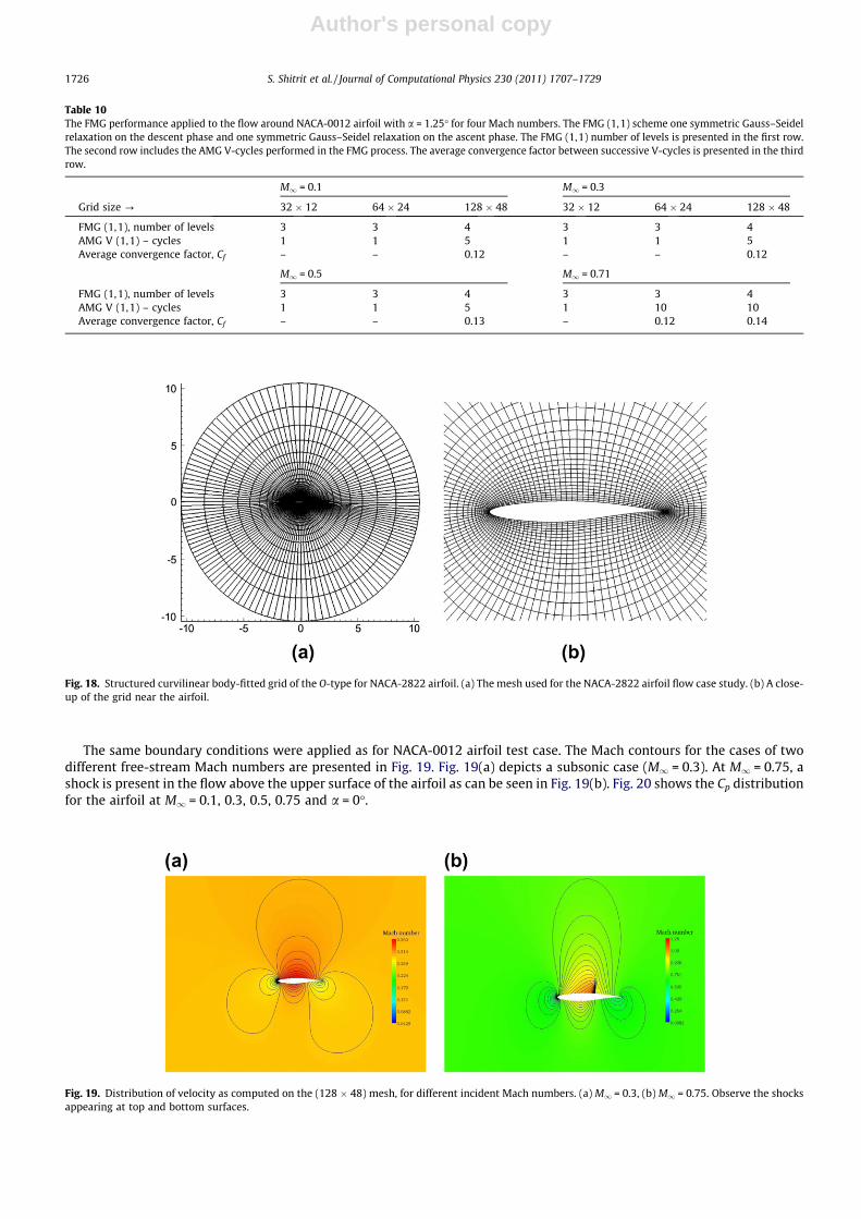
The same boundary conditions were applied as for NACA-0012 airfoil test case. The Mach contours for the cases of twodifferent free-stream Mach numbers are presented in Fig. 19. Fig. 19(a) depicts a subsonic case (M1 = 0.3). At M1 = 0.75, ashock is present in the flow above the upper surface of the airfoil as can be seen in Fig. 19(b). Fig. 20 shows the Cp distributionfor the airfoil at M1 = 0.1, 0.3, 0.5, 0.75 and a = 0�.

Table 10The FMG performance applied to the flow around NACA-0012 airfoil with a = 1.25� for four Mach numbers. The FMG (1,1) scheme one symmetric Gauss–Seidelrelaxation on the descent phase and one symmetric Gauss–Seidel relaxation on the ascent phase. The FMG (1,1) number of levels is presented in the first row.The second row includes the AMG V-cycles performed in the FMG process. The average convergence factor between successive V-cycles is presented in the thirdrow.

M1 = 0.1 M1 = 0.3

Grid size ? 32 � 12 64 � 24 128 � 48 32 � 12 64 � 24 128 � 48

FMG (1,1), number of levels 3 3 4 3 3 4AMG V (1,1) – cycles 1 1 5 1 1 5Average convergence factor, Cf – – 0.12 – – 0.12

M1 = 0.5 M1 = 0.71

FMG (1,1), number of levels 3 3 4 3 3 4AMG V (1,1) – cycles 1 1 5 1 10 10Average convergence factor, Cf – – 0.13 – 0.12 0.14

Fig. 18. Structured curvilinear body-fitted grid of the O-type for NACA-2822 airfoil. (a) The mesh used for the NACA-2822 airfoil flow case study. (b) A close-up of the grid near the airfoil.

Fig. 19. Distribution of velocity as computed on the (128 � 48) mesh, for different incident Mach numbers. (a) M1 = 0.3, (b) M1 = 0.75. Observe the shocksappearing at top and bottom surfaces.



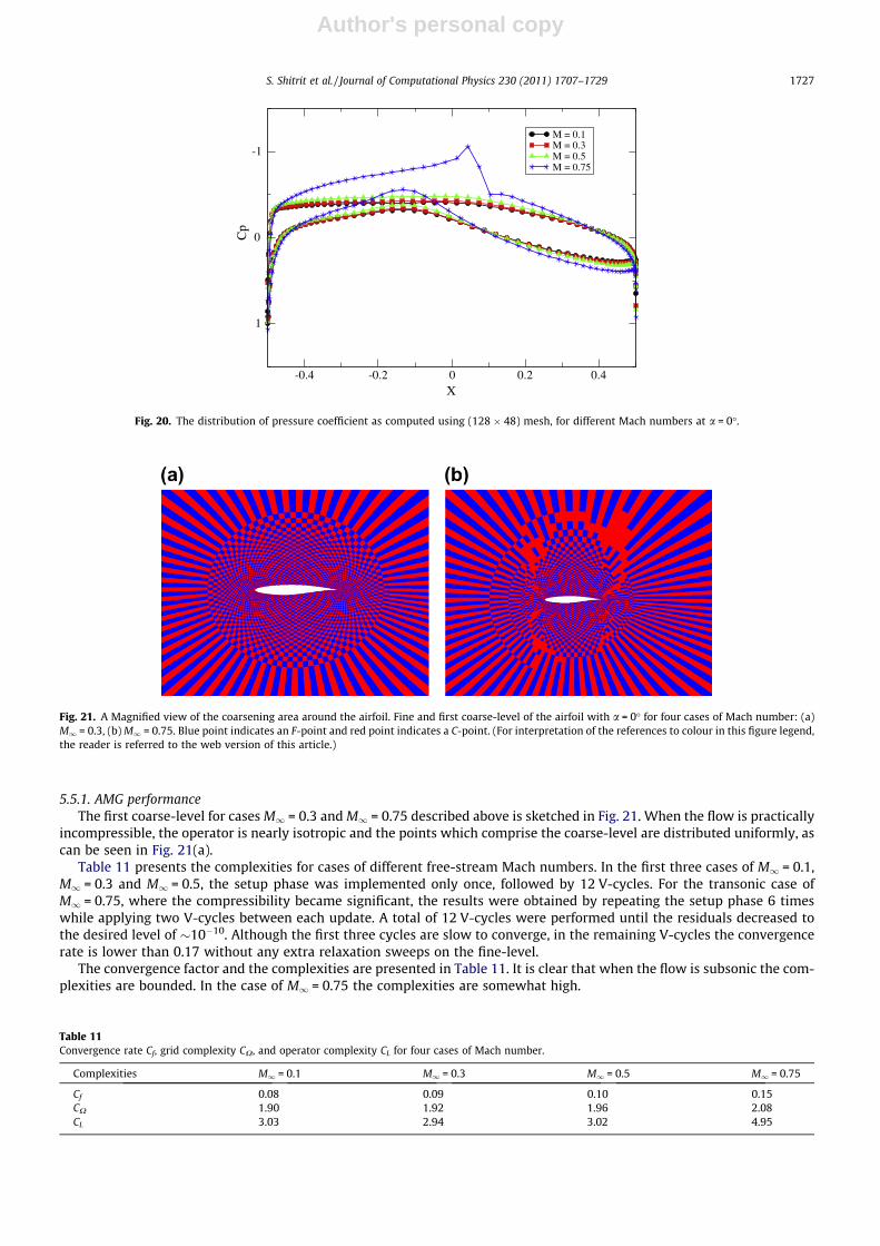
5.5.1. AMG performanceThe first coarse-level for cases M1 = 0.3 and M1 = 0.75 described above is sketched in Fig. 21. When the flow is practically

incompressible, the operator is nearly isotropic and the points which comprise the coarse-level are distributed uniformly, ascan be seen in Fig. 21(a).

Table 11 presents the complexities for cases of different free-stream Mach numbers. In the first three cases of M1 = 0.1,M1 = 0.3 and M1 = 0.5, the setup phase was implemented only once, followed by 12 V-cycles. For the transonic case ofM1 = 0.75, where the compressibility became significant, the results were obtained by repeating the setup phase 6 timeswhile applying two V-cycles between each update. A total of 12 V-cycles were performed until the residuals decreased tothe desired level of �10�10. Although the first three cycles are slow to converge, in the remaining V-cycles the convergencerate is lower than 0.17 without any extra relaxation sweeps on the fine-level.

The convergence factor and the complexities are presented in Table 11. It is clear that when the flow is subsonic the com-plexities are bounded. In the case of M1 = 0.75 the complexities are somewhat high.

-0.4 -0.2 0 0.2 0.4X

-1

0

1

Cp

M = 0.1M = 0.3M = 0.5M = 0.75

Fig. 20. The distribution of pressure coefficient as computed using (128 � 48) mesh, for different Mach numbers at a = 0�.

Fig. 21. A Magnified view of the coarsening area around the airfoil. Fine and first coarse-level of the airfoil with a = 0� for four cases of Mach number: (a)M1 = 0.3, (b) M1 = 0.75. Blue point indicates an F-point and red point indicates a C-point. (For interpretation of the references to colour in this figure legend,the reader is referred to the web version of this article.)

Table 11Convergence rate Cf, grid complexity CX, and operator complexity CL for four cases of Mach number.


Cf 0.08 0.09 0.10 0.15CX 1.90 1.92 1.96 2.08CL 3.03 2.94 3.02 4.95



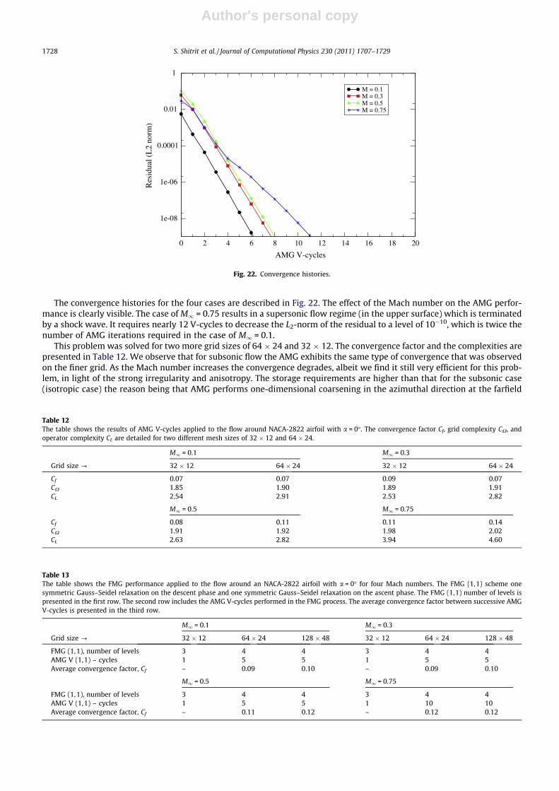
The convergence histories for the four cases are described in Fig. 22. The effect of the Mach number on the AMG perfor-mance is clearly visible. The case of M1 = 0.75 results in a supersonic flow regime (in the upper surface) which is terminatedby a shock wave. It requires nearly 12 V-cycles to decrease the L2-norm of the residual to a level of 10�10, which is twice thenumber of AMG iterations required in the case of M1 = 0.1.

This problem was solved for two more grid sizes of 64 � 24 and 32 � 12. The convergence factor and the complexities arepresented in Table 12. We observe that for subsonic flow the AMG exhibits the same type of convergence that was observedon the finer grid. As the Mach number increases the convergence degrades, albeit we find it still very efficient for this prob-lem, in light of the strong irregularity and anisotropy. The storage requirements are higher than that for the subsonic case(isotropic case) the reason being that AMG performs one-dimensional coarsening in the azimuthal direction at the farfield

0 2 4 6 8 10 12 14 16 18 20

AMG V-cycles

1e-08

1e-06

0.0001

0.01

1

Res

idua

l (L

2 no

rm)

M = 0.1M = 0.3M = 0.5M = 0.75


Table 12The table shows the results of AMG V-cycles applied to the flow around NACA-2822 airfoil with a = 0�. The convergence factor Cf, grid complexity CX, andoperator complexity CL are detailed for two different mesh sizes of 32 � 12 and 64 � 24.

M1 = 0.1 M1 = 0.3

Grid size ? 32 � 12 64 � 24 32 � 12 64 � 24

Cf 0.07 0.07 0.09 0.07CX 1.85 1.90 1.89 1.91CL 2.54 2.91 2.53 2.82

M1 = 0.5 M1 = 0.75

Cf 0.08 0.11 0.11 0.14CX 1.91 1.92 1.98 2.02CL 2.63 2.82 3.94 4.60

Table 13The table shows the FMG performance applied to the flow around an NACA-2822 airfoil with a = 0� for four Mach numbers. The FMG (1,1) scheme onesymmetric Gauss–Seidel relaxation on the descent phase and one symmetric Gauss–Seidel relaxation on the ascent phase. The FMG (1,1) number of levels ispresented in the first row. The second row includes the AMG V-cycles performed in the FMG process. The average convergence factor between successive AMGV-cycles is presented in the third row.

M1 = 0.1 M1 = 0.3

Grid size ? 32 � 12 64 � 24 128 � 48 32 � 12 64 � 24 128 � 48

FMG (1,1), number of levels 3 4 4 3 4 4AMG V (1,1) – cycles 1 5 5 1 5 5Average convergence factor, Cf – 0.09 0.10 – 0.09 0.10

M1 = 0.5 M1 = 0.75

FMG (1,1), number of levels 3 4 4 3 4 4AMG V (1,1) – cycles 1 5 5 1 10 10Average convergence factor, Cf – 0.11 0.12 – 0.12 0.12



since the strong connection in the n-direction (azimuthal direction) arises from a large grid spacing in g- direction. This facthas no adverse effect on the complexities.

Table 13 shows the FMG performance for cases of four different free-stream Mach numbers with mesh size of 128 � 48cells. In the case of M1 < 0.5 five AMG V-cycles were applied on each coarse-level as part of the FMG algorithm. Observe thatthe average convergence rate was around an order of magnitude per cycle. In the transonic case ten V-cycles were applied ineach coarse-levels.

6. Conclusions

Transonic flow problem is a rather complex one from a computational point of view. One of the main difficulties is the factthat the differential operator changes its type between elliptic for subsonic flow regime and hyperbolic (with respect to theflow direction) in the supersonic flow regime. Another (sub-) difficulty is that the subsonic flow regime itself presents twoextremities (and all the possible cases in between): nearly isotropic operator for the flow speed case and highly anisotropicoperator for a nearly sonic flow speed. While the standard AMG algorithm can treat the latter difficulty, it has never beenapplied yet, to the best of our knowledge, to the supersonic regime. The difficulties here begin with the fact that a simplepointwise relaxation procedure (a desirable component of AMG) appears unstable in the hyperbolic case. One of the mainachievements of our work is the development of a pointwise relaxation procedure that is stable (and constitutes a goodsmoother – in the algebraic sense) for both the subsonic and supersonic flow regimes. Second, we have constructed a variantof an AMG algorithm that employs the new relaxation procedure and allows to achieve very good convergence for both ellip-tic and hyperbolic cases.

A 2D body-fitted structured grid FPE solver which is based on the AMG method was developed. The flow solver is capableof resolving flows from subsonic to transonic and supersonic regimes. The flow solver can accommodate complex geome-tries. Several two dimensional flow calculations have been performed to test the performance of the algebraic multigridmethod. The computational method was demonstrated to be capable of predicting the shock formation and achieving resid-ual reduction of roughly an order of magnitude per cycle both for elliptic and hyperbolic problems, through the entire rangeof flow regimes, independent of the problem size (resolution). The purpose of this work was not to design an algorithmwhich is fine-tuned for a specific problem with the aim to obtain the highest possible efficiency, but a robust algorithmwhich can address most of the relevant cases regarding the FPE and achieve a good performance without tuning its param-eters any further. The AMG algorithm and all its components are constructed on the basis of compromise between the gen-eral applicability for the FPE and overall efficiency.

References

[1] E.M. Murman, J.D. Cole, Calculation of plane steady transonic flows, AIAA 9 (1) (1971) 114–121.[2] A. Brandt, Multigrid Techniques: 1984 Guide with Applications to Fluid Dynamics, The Weizmann Institute of Science, Rehovot, Israel, 1984.[3] I. Yavneh, Multigrid techniques for incompressible flows, PhD thesis, The Weizmann Institute of Science, Rehovot, Israel, 1991.[4] D. Sidilkover, A factorizable scheme for the equations of fluid flow, Appl. Numer. Math. 41 (2002) 423–426.[5] X.-C. Cai, W.D. Gropp, D.E. Keyes, R.G. Melvin, D.P. Young, Parallel Newton–Krylov–Schwarz algorithm for the transonic full potential equation, SIAM J.

Sci. Comput. 19 (1998) 246–265.[6] U. Trottenberg, A. Schuller, C.W. Oosterlee, Multigrid, Elsevier Academic Press, 2001.[7] P. Wesseling, An Introduction to Multigrid Methods, John Wiley & Sons, New York, 1992.[8] R.P. Fedorenko, The speed of convergence of one iterative process, USSR Comput. Math. Phys. 4 (1964) 227–235.[9] N.S. Bakhvalov, On the convergence of a relaxation method with natural constraints on the elliptic operator, USSR Comput. Math. Math. Phys. 6 (1966)

101.[10] A. Brandt, Multi-level adaptive technique (MLAT) for fast numerical solutions to boundary value problems, in: Proceedings of 3rd International

Conference on Numerical Methods in Fluids Mechanics, Lecture Notes in Physics, vol. 18, Springer-Verlag, 1973, pp. 82–89.[11] A. Brandt, Multi-level adaptive solutions to boundary-value problems, Math. Comput. 31 (1977) 333–390.[12] W. Hackbusch, Multigrid Methods and Applications, Springer, Heidelberg, 1985.[13] A. Brandt, S.F. McCormick, J.W. Ruge, Algebraic multigrid (AMG) for sparse matrix equations, in: Sparsity and Its Applications, Cambridge University

Press, Cambridge, 1984.[14] A. Brandt, Algebraic multigrid theory: the symmetric case, Appl. Math. Comput. 19 (1986) 23–56.[15] K. Stueben, An introduction to algebraic multigrid, Technical report, German National Research Center for Information Technology (GMD), San Diego,

2001.[16] J.W. Ruge, K. Stueben, Algebraic multigrid, in: S.F. McCormick (Ed.), Multigrid Methods, vol. 3, SIAM, Philadelphia, 1987, pp. 73–130.[17] S. Shitrit, D. Sidilkover, A full potential equation solver based on the algebraic multigrid method: elementary applications. J. Comput. Appl. Math., in

press.[18] S. Shitrit, D. Sidilkover, Toward applying algebraic multigrid to transonic flow problems, SIAM J. Sci. Comput. 32 (July) (2010) 2007–2028.[19] A. Jameson, Iterative solution of transonic flows over airfoils and wings, including flows at Mach 1, Pure Appl. Math. 27 (1974) 283–309.[20] S. Shitrit, D. Sidilkover, The discretization of the full potential equation, Comput. Fluids, in press.[21] S. Shitrit, Transonic flow computations by algebraic multigrid. PhD thesis, The Zandman-Slaner Graduate School of Engineering, Tel-Aviv University,

Tel-Aviv Univeristy, July 2010.[22] W.L. Briggs, V.E. Henson, S.F. McCormick, A Multigrid Tutorial, 2 ed., Society for Industrial and Applied Mathematics, Philadelphia, 2000.[23] R.D. Falgout, An introduction to algebraic multigrid, in: Computer in Science Engineering, Lawrence Livermore National Laboratory, 2006.[24] Q. Chang, Y. Shu, Wong H. Fu, On the algebraic multigrid, J. Comput. Phys. 125 (1996) 279–292.[25] A.H. Shapiro, The Dynamics and Thermodynamics of Compressible Fluid Flow, vol. 1, John Wiley & Sons, New York, 1953.[26] J.D. Anderson, Modern Compressible Flow: With Historical Perspective, McGraw-Hill series in aeronautical and aerospace engineering, 2003.[27] D. Hawken, 2009. Available from <www.telusplanet.net>.


An algebraic multigrid solver for transonic flow problems

Documents