An algebraic approach for modeling and simulation of road traffic networks

An algebraic approach for modeling and simulation of

road traffic networks

Nadir Farhi*,1, Habib Haj-Salem1

and Jean-Patrick Lebacque1

1 Université Paris-Est, IFSTTAR/COSYS/GRETTIA, F-77447 Champs-sur Marne Cedex France

Abstract. We present in this article an algebraic approach to model and

simulate road traffic networks. By defining a set of road traffic systems and

adequate concatenating operators in that set, we show that large regular road

networks can be easily modeled and simulated. We define elementary road

traffic systems which we then connect to each other and obtain larger systems.

For the traffic modeling, we base on the LWR first order traffic model with

piecewise-linear fundamental traffic diagrams. This choice permits to represent

any traffic system with a number of matrices in specific algebraic structures.

For the traffic control on intersections, we consider two cases: intersections

controlled with a priority rule, and intersections controlled with traffic lights.

Finally, we simulate the traffic on closed regular networks, and derive the

macroscopic fundamental traffic diagram under the two cases of intersection

control.

Keywords: Road traffic modeling and simulation, min-plus algebra, traffic

control.

1 Introduction

Modeling the traffic in urban networks is necessary to understand the vehicular

dynamics and set adequate strategies and controls, in order to improve the service.

Many models with different approaches exist in the literature (1). We present in this

article a urban traffic model based in the cell-transmission model (2) (a numerical

scheme of the first order macroscopic LWR model (3), (4)); see also (5). The model

adapts the existing approach to the urban traffic framework. Moreover, two models of

intersection control are proposed. An algebraic formulation of the whole vehicular

dynamics in a urban road network is made. The formulation permits to represent the

traffic dynamics in the network by a number of matrices in the min-plus algebra (a

specific algebraic structure) (6).

The approach we adopt here is a system theory approach, where the urban traffic

network is build from predefined elementary traffic systems and adequate operators,

for the connection of these systems. We first present the link traffic model inspired

from the cell-transmission model (2), with its algebraic formulation. In section 3, we

* Corresponding author ([email protected])

give two intersection traffic models. In section 4, we explain the algebraic

construction of an American-like (regular) city, by giving the three elementary traffic

systems and the main operator we use for that. In the last part of the article we present

some numerical traffic simulations on regular cities set on a torus (closed networks).

This configuration permits to easily derive the macroscopic fundamental diagram on

such networks. Finally, we discuss the traffic phases obtained from those diagrams,

under two control policies set on the intersections. In this article, we only review the

traffic models we use. For more details on those models; see (8), (9), (10) and (12).

The main contribution of this article is the system theory approach we propose for

building and simulating urban traffic networks.

2 The link model

The model we propose here is based on the macroscopic first order LWR model (3)

(4), with triangular fundamental diagrams, where the dynamics of vehicle pelotons

moving through road sections is described. We assume here that only pelotons are

observed. Moreover, the density of pelotons is considered to be binary, in the sense

that, at a given time, the density on a given section is equal to 1 if any peloton of

vehicles is moving on, and it is equal to zero otherwise. We think that this mesoscopic

representation of the traffic dynamics is convenient to describe the traffic in urban

networks.

Figure 1. A single-lane road.

We first present the traffic model on a single link, where traffic is unidirectional,

and where vehicles move without passing. Let us explain the traffic dynamics on a

road of m sections. We use the following notations.

𝑛𝑖(𝑡) ∈ 0,1 : number of pelotons in section 𝑖, at time 𝑡, with 𝑖 =1,2,… ,𝑛 and 𝑡 ∈ ℕ.

𝑛 𝑖 𝑡 = 1 − 𝑛𝑖(𝑡) ∈ 0,1 : free space in section 𝑖 at time 𝑡, with 𝑖 =1,2,… ,𝑛 and 𝑡 ∈ ℕ.

𝑄0(𝑡) ∈ ℕ: Cumulated flow (in number of pelotons per time unit) from

time zero to time 𝑡, of vehicle pelotons entering to section 1.

𝑄𝑖 𝑡 ∈ ℕ, 𝑖 = 1,2,… ,𝑛 − 1: Cumulated flow from time zero to time 𝑡, of

vehicle pelotons passing from section 𝑖 to section 𝑖 + 1.

𝑄𝑚 (𝑡) ∈ ℕ: Cumulated flow from time zero to time 𝑡, of vehicle pelotons

leaving section 𝑚.

We assume here triangular fundamental diagrams on all the road sections.

𝑞𝑖 = min 𝑣𝑖 𝜌𝑖 ,𝑤𝑖 𝜌𝑖𝑗− 𝜌𝑖 . (1)

where 𝑞𝑖 ,𝜌𝑖 , 𝑣𝑖 ,𝑤𝑖 and 𝜌𝑖𝑗 denote respectively, the car-flow, the car-density, the

free speed, the backward wave speed, and the jam density, in section 𝑖. We assume

that all sections have the same fundamental diagram. Moreover, according to the

assumptions above, we assume that 𝑣𝑖 = 𝑤𝑖 = 𝜌𝑖𝑗

= 1,∀𝑖 = 1,2,… ,𝑚. We thus

obtain the following fundamental diagram for all the sections.

𝑞𝑖 = min 𝜌𝑖 , 1 − 𝜌𝑖 (2)

According to the cell-transmission model (2) (7), which is a convenient numerical

scheme of the LWR macroscopic model (3) (4), the traffic demand and supply are

derived from the fundamental traffic diagram, and are given as follows.

𝛿𝑖 𝑡 = min 𝑣𝑖𝜌𝑖(𝑡), 𝑞𝑖𝑚𝑎𝑥 = min(𝜌𝑖(𝑡),1/2) : the traffic demand from

section 𝑖 to section 𝑖 + 1 at time t.

𝜎𝑖 𝑡 = min(𝑞𝑖𝑚𝑎𝑥 ,𝑤𝑖 𝜌𝑖

𝑗− 𝜌𝑖 𝑡 = min(1/2, 1 − 𝜌𝑖(𝑡)) : the traffic

supply of section 𝑖 to section 𝑖 − 1.

where

𝑞𝑖𝑚𝑎𝑥 =

𝜌𝑗1𝑣𝑖

+1𝑤𝑖

=1

2,∀𝑖 = 1,2,… ,𝑚.

(3)

The cumulated traffic demand in the entry of the road, denoted by ∆0(𝑡), as well as

the cumulated traffic supply on the exit of the road, denoted by 𝛴𝑛+1(𝑡) are supposed

to be given over the whole time. They represent the boundary conditions of the

system. The initial traffic condition consists here in giving the densities 𝜌𝑖 0 , 𝑖 =1,2,… ,𝑚 (the densities on each road section at time zero).

We assume that all the sections of the road have the same length, which we denote

by ∆𝑥. Moreover, we fix the time unit 𝑑𝑡 to 𝑑𝑡 = ∆𝑥/𝑣 = ∆𝑥/𝑤. The model consists

finally in giving the dynamics of the cumulated flows 𝑄𝑖 𝑡 , 𝑖 = 0,1,… ,𝑚 over time

𝑡 ∈ ℕ.

𝑄0 𝑡 + 𝑑𝑡 = min ∆0 𝑡 ,𝑄1 𝑡 + 𝑛 1 0

𝑄𝑖 𝑡 + 𝑑𝑡 = min 𝑄𝑖−1 𝑡 + 𝑛𝑖 0 ,𝑄𝑖+1 𝑡 + 𝑛 𝑖+1 0

𝑄𝑚 𝑡 + 𝑑𝑡 = min 𝑄𝑚−1 𝑡 + 𝑛𝑚 0 ,𝛴𝑛+1 𝑡

(4)

and, by that, updating the number of pelotons 𝑛𝑖 𝑡 , 𝑖 = 1,2,… ,𝑛; 𝑡 ∈ ℕ.

𝑛𝑖 𝑡 = 𝑛𝑖 0 + 𝑄𝑖−1 𝑡 − 𝑄𝑖 𝑡 , 𝑖 = 1,2,… ,𝑛. (5)

Let us notice that we assume here that the cumulated flows are initialized to zero:

𝑄𝑖 0 = 0,∀𝑖 = 0,1,… ,𝑚.

Algebraic formulation

We consider here the algebraic structure ℝ𝑚𝑖𝑛 ≔ ℝ ∪ +∞ ,⊕,⊗ , where the

operations ⊕ and ⊗ are defined as follows.

𝑎 ⊕ 𝑏 ≔ min 𝑎, 𝑏 , ∀𝑎, 𝑏 ∈ ℝ𝑚𝑖𝑛

𝑎 ⊗ 𝑏 ≔ 𝑎 + 𝑏, ∀𝑎, 𝑏 ∈ ℝ𝑚𝑖𝑛

The structure ℝ𝑚𝑖𝑛 is a dioid (an idempotent semiring); see (6). We denote by

휀 = +∞ and 𝑒 = 0 respectively the zero and the unity elements for ℝ𝑚𝑖𝑛 . We have

also a dioid in the set ℳ𝑛×𝑛(ℝ𝑚𝑖𝑛 ) of square matrices with elements in ℝ𝑚𝑖𝑛 , where

the operations ⊕ and ⊗ are defined as follows.

(𝐴 ⊕ 𝐵)𝑖𝑗 ≔ 𝐴𝑖𝑗 ⊕𝐵𝑖𝑗 = min 𝐴𝑖𝑗 ,𝐵𝑖𝑗 , ∀𝐴,𝐵 ∈ ℳ𝑛×𝑛(ℝ𝑚𝑖𝑛 )

(𝐴 ⊗ 𝐵)𝑖𝑗 ≔ ⊕1≤𝑘≤𝑛

𝐴𝑖𝑘 ⊗𝐵𝑘𝑗 = min1≤𝑘≤𝑛

(𝐴𝑖𝑘 + 𝐵𝑘𝑗 ), ∀𝐴,𝐵 ∈ ℳ𝑛×𝑛 ℝ𝑚𝑖𝑛 .

It is then easy to check that the dynamics (4) can be written as follows.

𝑄(𝑡 + 𝑑𝑡) = 𝐴⊗𝑄(𝑡) ⊕𝑏(𝑡) (6)

where 𝑄(𝑡) is the vector whose components are the cumulated flows 𝑄𝑖(𝑡), and

where 𝐴 ∈ ℳ𝑛×𝑛 ℝ𝑚𝑖𝑛 and 𝑏(𝑡) ∈ ℳ1×𝑛 ℝ𝑚𝑖𝑛 are given as follows.

𝐴 =

휀 𝑛 1(0) 휀 ⋯ ⋯ 휀𝑛1(0) 휀 𝑛 2(0) 휀 ⋯ 휀

휀 𝑛2(0) 휀 𝑛 3(0) 휀

⋮ ⋱ ⋱ ⋱ ⋮𝑛𝑚−1(0) 휀 𝑛 𝑚 (0)

𝑛𝑚 (0) 휀

, 𝑏 𝑡 =

∆0 𝑡 휀휀⋮휀

𝛴𝑛+1 𝑡

.

with 𝑄 0 = 0.

With this formulation, the traffic model on any single-lane road is summarized by

the two matrices 𝐴 and 𝑏(𝑡), t∈ ℕ. The simulation of the traffic model is then simply

done by iterating the min-plus linear dynamics (6), with the initial condition 𝑄(0) =0. We notice that the matrix 𝐴 and the vector 𝑏(𝑡) contain respectively the initial

condition (initial density) and the boundary conditions (demand inflow and supply

outflow). For more details on the model presented in this section, see (8) (9). We will

see below (in the two dimensional traffic modeling section), that the linearity of the

traffic dynamics obtained in the one dimension model cannot be preserved.

3 Two dimensional traffic modeling

In order to be able to model the traffic on road networks, we need to have models for

intersections. We present in this section two models. The first model describes the

traffic inflowing to and out-flowing from an intersection with two entry roads and two

exit roads where one of the entry roads has priority with respect to the other one. The

second model considers that the intersection is controlled with a traffic light.

Figure 2. Intersection of two roads.

3.1 Intersection model with a priority rule.

Let us consider the intersection of Figure 2, where a priority rule is set. Vehicles

entering the intersection from road 1 (the North) have priority with respect to vehicles

entering the intersection from road 2 (the West). 𝑛0(𝑡) and 𝑛 0(𝑡) denote respectively

the number of pelotons and the free space in the intersection at time 𝑡. Equations (7)

below only describe the traffic dynamics on the intersection. The traffic on the roads

follows the dynamics described above.

𝑄1𝑚 𝑡 + 𝑑𝑡 = min 𝑄1𝑚−1 𝑡 + 𝑛1𝑚 0 ,𝑄31 𝑡 + 𝑄41 𝑡 − 𝑄2𝑚 𝑡 + 𝑛 0 0

𝑄2𝑚 𝑡 + 𝑑𝑡 = min 𝑄2,𝑚−1 𝑡 + 𝑛2,𝑚 0 ,𝑄31 𝑡 + 𝑄41 𝑡 − 𝑄1𝑚 𝑡 + 𝑑𝑡 + 𝑛 0 0

𝑄31 𝑡 + 𝑑𝑡 = min 𝛼13𝑄1𝑚 𝑡 + 𝛼23𝑄2𝑚 𝑡 + 𝑛0 0 ,𝑄32 𝑡 + 𝑛 31 0

𝑄41 𝑡 + 𝑑𝑡 = min 𝛼14𝑄1𝑚 𝑡 + 𝛼24𝑄2𝑚 𝑡 + 𝑛0 0 ,𝑄42 𝑡 + 𝑛 41 0

(7)

where the notations used in (7) are (see Figure 2):

𝑄1𝑚 𝑡 : cumulated outflow from road 1, which is also the cumulated

inflow to the intersection, from the north side, up to time 𝑡. 𝑄2𝑚 𝑡 : cumulated outflow from road 2, which is also the cumulated

inflow to the intersection, from the west side, up to time 𝑡. 𝑄31 𝑡 : cumulated outflow from the intersection to the south, which is

also the cumulated inflow to road 3, up to time 𝑡.

𝑄41 𝑡 : cumulated outflow from the intersection to the east, which is also

the cumulated inflow to road 4, up to time 𝑡. The dynamics of 𝑄1𝑚 and 𝑄2𝑚 in (7) (the two first equations) set the priority to the

outflow from road 1 with respect to the outflow from road 2. This is done by the

introduction of an implicit term in the dynamics of 𝑄2𝑚 in (7). For more details, see

(8) (9) (10).

Using the same notations as above, we can easily check that the dynamics (7) is

written with matrix notations as follows.

𝑄 𝑡 + 𝑑𝑡 = D ⊗ H Q t + G Q t + dt ⊕ 𝑏 𝑡 (8)

where 𝐷 is a min-plus matrix, and 𝐻 and 𝐺 are standard matrices. The matrices 𝐻

and 𝐺 contain multipliers that cannot be expressed linearly in the min-plus algebra.

These multipliers are needed to model the turning rates as well as the priority rule at

the intersection. The turning rates in the level of the intersection are given by 𝐻 and

𝐺, where 𝐻 gives the turning rates with a time delay 𝑑𝑡, and 𝐺 gives the turning rates

without any time delay (the implicit term setting the priority rule). For more details on

the model presented in this section, see (8) (9) (10).

3.2 Intersection model with a traffic light control.

We give in this section the traffic dynamics in the case where the intersection is

managed by means of a traffic light. In a first step, we consider only the case where

an open loop control is set on the traffic light. The control is assumed to be periodic

with a time period (cycle) denoted by 𝑐 (which is in fact equal to 𝑐 𝑑𝑡). The green

times for the north and the west sides are denoted respectively by 𝑔𝑁 and 𝑔𝑊. The

integral red times between the two green times are denoted by 𝑟1 and 𝑟2respectively

for the integral red time from the end of 𝑔𝑁 and the beginning of 𝑔𝑊 and for the

integral red time from the end of 𝑔𝑊 and the beginning of 𝑔𝑁; see Figure 3.

Figure 3. Time cycle for the traffic light.

The dynamics (7) is modified to:

𝑄1𝑚 𝑡 + 𝑑𝑡 = min

𝑄1𝑚−1 𝑡 + 𝑛1𝑚 0 ,

𝑄31 𝑡 + 𝑄41 𝑡 − 𝑄2𝑚 𝑡 + 𝑛 0 0 ,

𝑄1𝑚 𝑡 + 𝐿1 .

𝑄2𝑚 𝑡 + 𝑑𝑡 = min

𝑄2,𝑚−1 𝑡 + 𝑛2,𝑚 0 ,

𝑄31 𝑡 + 𝑄41 𝑡 − 𝑄1𝑚 𝑡 + 𝑛 0 0 ,

𝑄2𝑚 𝑡 + 𝐿2 .

𝑄31 𝑡 + 𝑑𝑡 = min 𝛼13𝑄1𝑚 𝑡 + 𝛼23𝑄2𝑚 𝑡 + 𝑛0 0 ,𝑄32 𝑡 + 𝑛 31 0

𝑄41 𝑡 + 𝑑𝑡 = min 𝛼14𝑄1𝑚 𝑡 + 𝛼24𝑄2𝑚 𝑡 + 𝑛0 0 ,𝑄42 𝑡 + 𝑛 41 0

(9)

where 𝐿1 = 𝑞1,𝑚𝑚𝑎𝑥 =

1

2 𝑖𝑓 𝑡 ∈ 𝑘𝑐, 𝑘𝑐 + 𝑔𝑁 ,

0 𝑜𝑡𝑕𝑒𝑟𝑤𝑖𝑠𝑒

and 𝐿2 = 𝑞2,𝑚𝑚𝑎𝑥 =

1

2 𝑖𝑓 𝑡 ∈ 𝑘𝑐 + 𝑔𝑁 + 𝑟1 , 𝑘𝑐 + 𝑔𝑁 + 𝑟1 + 𝑔𝑊 ,

0 𝑜𝑡𝑕𝑒𝑟𝑤𝑖𝑠𝑒

Thus, in the time instants when 𝐿1 = 𝑞1,𝑚𝑚𝑎𝑥 = 1/2, the traffic light is green for the

road 1, because, 𝑄1,𝑚 (𝑡) may be increased by 𝑞1,𝑚𝑚𝑎𝑥 , under the two constraints of

upstream demand and downstream supply. In the time instants when 𝐿1 = 0, the

traffic light is red for road 1, because, 𝑄1,𝑚 (t) stays constant, i.e. 𝑄1,𝑚 𝑡 + 𝑑𝑡 =

𝑄1,𝑚 (𝑡). The same reasoning is made for the road 2. The algebraic formulation of the

model (9) is similar to the one done in (8), but we need here to define four dynamics,

one for each phase of the time cycle. For more details in the model presented in this

section, see (8) (10) (9).

4 An American-like city We define in this section a set of dynamic systems such that any traffic system

defined under the models presented above, is contained in that set. We also define

operators for the connection of those systems. The systems we consider here are those

with two vectors of input signals 𝑈 and 𝑉, two vectors of state signals 𝑃 and 𝑄, and

two vectors of output signals 𝑌 and 𝑍, such that we can write

𝑃(𝑡 + 𝑑𝑡)

𝑄 𝑡 + 𝑑𝑡

𝑌(𝑡 + 𝑑𝑡)

𝑍(𝑡 + 𝑑𝑡)

=

0 𝐴 0 𝐵𝐶 휀 𝐷 휀0 𝐸 0 0𝐹 휀 휀 휀

⊠

P t + dt

Q t

U(t + dt)

V(t)

≔

AQ t + BV t

C ⊗ P t + dt ⊕ D ⊗ U t + dt

EQ(t)

F ⊗ V(t)

,

(10)

where 𝐴,𝐵 and 𝐸 are standard matrices, while 𝐶,𝐷 and 𝐹 are min-plus matrices.

This construction is inspired from Petri Net modeling, see (8). If we denote by 𝑆 the

system (10), then we write 𝑌,𝑍 = 𝑆(𝑈,𝑉). Let us explain how traffic dynamics

given above are written in the form (10). For that, we first do it for the three

elementary systems on which we will base for building traffic systems of large

networks. The three elementary systems that we consider here are the following.

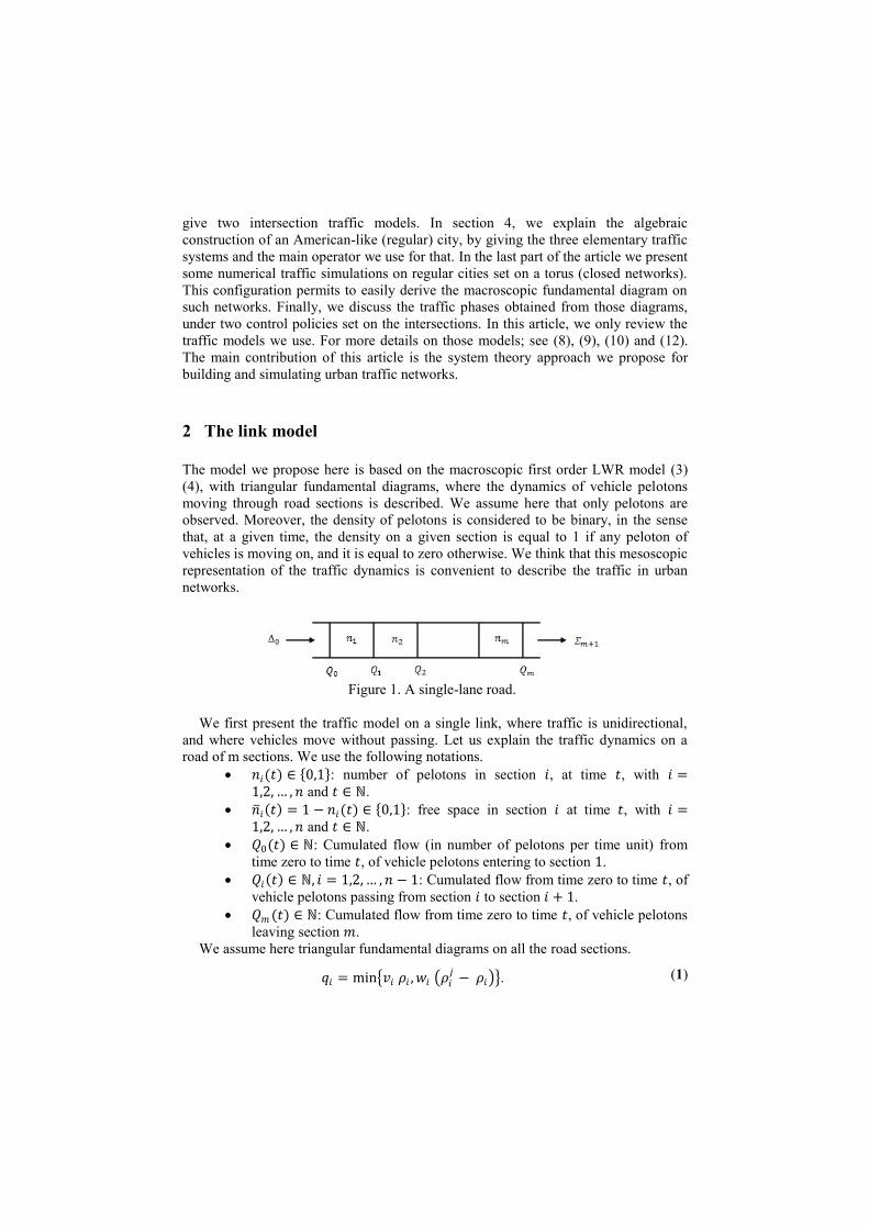
(a) (b) (c)

Figure 4. Elementary traffic systems: (a) a road section, (b) an intersection entry, (c)

an intersection exit.

a) a road section is the elementary traffic system in a road. The system has

two input signals 𝑈and 𝑉, one state signal 𝑄, and two output signals 𝑌

and 𝑍.

b) an intersection entry is a special road section with more output signals

than an ordinary road section (a). The system has two input signals 𝑈and

𝑉, one state signal 𝑄, and three output signals 𝑌,𝑍1 and 𝑍2.

c) an intersection exit is a special road section with more output signals than

an ordinary road section (a). The system has two input signals 𝑈and 𝑉,

one state signal 𝑄, and three output signals 𝑌1 ,𝑌2 and 𝑍.

In order to clarify how the dynamics of these elementary systems are written in the

form (10), we explain the dynamics of a road section (system (a)). Following the

dynamics (4) (or (6)), the dynamics of the road section (a) is written as follows.

𝑄 𝑡 + 𝑑𝑡 = min 𝑛 0 + 𝑉 𝑡 ,𝑈 𝑡 + 𝑑𝑡 ,

𝑌 𝑡 + 𝑑𝑡 = 𝑄 𝑡 + 𝑑𝑡 ,

𝑍 𝑡 + 𝑑𝑡 = 𝑛 0 + 𝑄 𝑡 .

(11)

Then by introducing intermediate variables, we get

𝑃1 𝑡 + 𝑑𝑡 = 𝑉(𝑡 + 𝑑𝑡)

𝑃2 𝑡 + 𝑑𝑡 = 𝑄(𝑡 + 𝑑𝑡)

𝑄 𝑡 + 𝑑𝑡 = min 𝑛 0 + 𝑃1 𝑡 ,𝑈 𝑡 + 𝑑𝑡 ,

𝑌 𝑡 + 𝑑𝑡 = 𝑄 𝑡 + 𝑑𝑡 ,

𝑍 𝑡 + 𝑑𝑡 = 𝑛 0 + 𝑃2 𝑡 .

(12)

Which can be easily written in the form (10) with

𝑃 = 𝑃1

𝑃2 ,𝐴 =

01 ,𝐵 =

10 ,𝐶 = 𝑛(0) 휀 ,𝐷 = 𝑒,𝐸 = 1,𝐹 = 휀 𝑛 0 .

Figure 5. Connection of traffic elementary systems.

The dynamics of the two systems (b) and (c) are obtained in the similar way. Let us

now explain how the systems are connected. For this, we define below the operator

used for the connection. In figure 5, we illustrate the connection of road sections, and

the construction of an intersection. Let us notice that an intersection is composed of

two intersection entries and two intersection exits.

Connection of systems

Connecting two system 𝑆1 and 𝑆2 consists in equaling a part of inputs of each

system with a part of outputs of the other system. We thus need first to specify the

parts of inputs and outputs to be equalized. Let us note 𝑆1𝑌,𝑍,𝑌 ′ ,𝑍′𝑈 ,𝑉,𝑈 ′ ,𝑉′

and 𝑆2𝑌,Z",𝑈′ ,𝑉′𝑈,V,𝑌 ′ ,𝑍′ ,

where 𝑈′ ,𝑉′ are inputs for 𝑆1, and outputs for 𝑆2, while 𝑌′ ,𝑍′ are inputs for 𝑆2 and

outputs for 𝑆1.The connection of the two systems 𝑆1 and 𝑆2, denoted simply by 𝑆1𝑆2,

is the system 𝑆 𝑌 ,𝑍,𝑌",𝑍"𝑈,𝑉 ,𝑈",𝑉"

given as the solution, on 𝑌,𝑌",𝑍,𝑍", of the system

𝑌𝑌′ ,𝑍𝑍′ = 𝑆1(𝑈𝑈′ ,𝑉𝑉 ′)

𝑈′𝑌,V'Z = 𝑆2(𝑌′𝑈",𝑍′𝑉")

Then, if we partition the input matrices of both systems 𝑆1 and 𝑆2 as follows

𝐵1𝐵′1 , 𝐵′

2𝐵"2 , 𝐷1𝐷′1 , [𝐷′2𝐷"2]

and the output matrices of the systems as follows

𝐸1

𝐸′1 ,

𝐸′2𝐸"2

, 𝐹1

𝐹′1 ,

𝐹′ 2

𝐹"2 ,

then the system 𝑆 is given by the matrices 𝐴 ,𝐵 ,𝐶 ,𝐷 ,𝐸 and 𝐹

𝐴 =

𝐴1 0 0 𝐵′1

0 𝐴2 𝐵′2 0

𝐸1 0 0 0

0 𝐸′2 0 0

,𝐵 =

𝐵1 00 𝐵"2

0 00 0

,𝐶 =

𝐶1 휀 휀 𝐷′1

휀 𝐶2 𝐷′2 휀

𝐹′1 휀 휀 휀

휀 𝐹′ 2 휀 휀

,

𝐷 =

𝐷1 휀휀 𝐷"2

휀 휀휀 휀

,𝐸 = 𝐸1 0 0 00 𝐸"2 0 0

,𝐹 = 𝐹1 휀 휀 휀휀 𝐹"2 휀 휀

.

For more details on this construction see (8).

Closed loop control.

We present in this section the application of an existing centralized urban control

strategy, which is called TUC (Traffic Urban Control), see (11). The objective here is

to derive the macroscopic fundamental traffic diagram on a regular city, under this

control strategy, and then compare it to the diagrams obtained under the open loop

control presented above, and under the priority rule.

TUC strategy assumes given a nominal traffic state (vehicle densities on the roads

and controls in intersections), and regulates the traffic in the urban network, around

the nominal traffic state. Let us use the notations.

𝑥𝑖(𝑡): the number of vehicles moving on raod 𝑖 at time 𝑡. 𝑥 𝑖 : nominal number of vehicles moving on road 𝑖. 𝑢𝑖(𝑡): outflow from road 𝑖 at time 𝑡. 𝑢 𝑖 : nominal outflow from road 𝑖. We then solve the following linear quadratic control problem.

min𝑢∈𝑈

𝑥 𝑡 − 𝑥 ′𝑄 𝑥 𝑡 − 𝑥 + 𝑢 𝑡 − 𝑢 ′𝑅 𝑢 𝑡 − 𝑢

+∞

𝑡=0

𝑥 𝑡 + 𝑑𝑡 − 𝑥 = 𝑥 𝑡 − 𝑥 + 𝐵 𝑢 𝑡 − 𝑢 .

(13)

For example, according to Figure 2, the dynamics of the number of vehicles

moving on the road 4 is written

𝑥4 𝑡 + 𝑑𝑡 = 𝑥4 𝑡 + 𝛼14𝑢1 𝑡 + 𝛼24𝑢2 𝑡 − 𝑢4(𝑡). (14)

For more details on this approach, see (11) (8).

5 Simulation and derivation of macroscopic fundamental diagram

Following the models presented in the sections above, we build a regular city (an

American-like city, where parallel horizontal avenues with alternated senses intersect

parallel vertical avenues with alternated senses, see Figure 6). Without loss of

generality, we assume here that the city is wholly symmetric, in the sense that all

roads have the same length, the same fundamental traffic diagram, and all the turning

rates are equal to 1/2. Because of the symmetry, the ideal control in this configuration

would be to uniformly distribute the number of cars on the roads of the city.

The objective of considering closed networks, like a city on a torus (Figure 6) is to

be able to fix the car density on the whole network, and then derive the asymptotic

average car-flow on the whole network. Theoretical results on the existence and

uniqueness of such asymptotic average flows, as well as their dependence on the

initial average car-density in the network, can be found in (8) (12).

Figure 6. A regular city (left side), and a regular city on a torus.

In Figure 7 we give the fundamental traffic diagrams (average traffic flow in

function of the average traffic density on the city) derived from the whole city on a

torus, under different control strategies on the intersections.

Figure 7. Comparison of the fundamental traffic diagrams obtained under different

control policies set on the intersections of the regular city on a torus.

1. Priority rule. 2. Traffic lights in open loop, with equal green times for both

directions of every intersection. 3. Local feedback that sets green times on every

intersection, proportional to the densities on the two entering roads. 4. Centralized

feedback control with TUC strategy.

In Figure 8, we show some simulations of traffic on the regular city on a torus. In

particular, we compare in that figure the control of traffic lights under open loop and

centralized closed loop controls. The result is that the centralized closed loop control

is the better strategy, in the sense that it attains surely the nominal traffic state, which

is here the uniform distribution of the number of cars on the roads of the city. This is

also confirmed on the fundamental diagrams of Figure 7, where only the centralized

feedback strategy guaranties acceptable flows in the case of high densities.

Figure 8. Traffic simulation. On the left side: open loop control. On the right side:

centralized closed loop control.

6 Conclusion

The traffic modeling approach we proposed in this article permits to algebraically

build large urban regular networks, such as American-like cities. Two intersection

models are presented: intersection managed with a priority rule, and intersection

controlled with a traffic light. Moreover, a centralized feedback control is applied to

control such road networks. Finally we compared different control approaches by

means of the derived macroscopic fundamental diagrams. The conclusion is that

centralized feedback controls are the better control strategies for the stabilization of

the traffic under severe congestion.

References

1. Transportation Research Part B,C.

2. Daganzo, C. F. The cell transmission model: A dynamic representation of highway traffic

consistent with the hydrodynamic theory. Transportation Research Part B: Methodological,

28(4), 269-287, 1994. pp. 269-287.

3. Lighthill, M. J. and Whitham, J. B. On kinematic waves II: A theory of traffic flow on long

crowded roads. Proceedings of the Roayl Society A, 1955.

4. Richards, P. I. Shockwaves on the highway. Operations Research, 1956.

5. Lebacque, J.-P. The Godunov scheme and what it means for the first order traffic flow

models. In: Lesort, J.-B. (Ed.), Proceedings of the 13th ISTTT, 647-678., 1996.

6. Baccelli, Francois, et al. Synchronization and Linearity. Wiley, 1992.

7. Daganzo, C. F. The cell transmission model, Part II: Network traffic. Transportation

research Part B, 29(2), 79-93, 1995.

8. Farhi, N. Modélisation minplus et commande du trafic de villes régulières. PhD thesis,

University of Paris 1 Panthéon - Sorbonne, 2008.

9. Farhi, N., Goursat, M. and Quadrat, J.-P. Derivation of the fundamental traffic diagram for

two circular roads and a crossing using minplus algebra and Petri net modeling. in

Proceedings of the IEEE Conference on Decision and Control, 2005.

10. Farhi, N. Modeling and control of elementary 2D-Traffic systems using Petri nets and

minplus algebra. in the Proceedings of the IEEE Conference on Decision and Control,

2009. pp. 2292-2297.

11. Diadaki, C., Papageorgiou, M. and Aboudolas, K. A multivariable regulator approach to

traffic-responsive network-wide signal control. Control Eng. Practice, 2002.

12. Farhi, N., Goursat, M. and Quadrat, J.-P. The traffic phases of road networks.

Transportation Research Part C, Volume 19, Issue 1., 2011. pp. 85-102.