An adaptive middleware for supporting time-critical event response

Cluster Comput (2009) 12: 87–100DOI 10.1007/s10586-008-0071-x

An adaptive middleware for supporting time-critical eventresponse

Qian Zhu · Gagan Agrawal

Received: 7 October 2008 / Accepted: 9 October 2008 / Published online: 6 November 2008© Springer Science+Business Media, LLC 2008

Abstract There are many applications where a timely re-sponse to an important event is needed. Often such responsecan require significant computation and possibly communi-cation, and it can be very challenging to complete it withinthe time-frame the response is needed. At the same time,there could be application-specific flexibility in the compu-tation that may be desired.

This paper presents the design, implementation, and eval-uation of a middleware that can support such applications.Each of the services in our target applications could have oneor more service parameters, which can be modified, withinthe pre-specified ranges, by the middleware. The middle-ware enables the time-critical event handling to achievethe maximum benefit, as per the user-defined benefit func-tion, while satisfying the time constraint. Our middleware isalso based on the existing Grid infrastructure and Service-Oriented Architecture (SOA) concepts. We have evaluatedour middleware and its support for adaptation using a vol-ume rendering application and a Great Lake forecasting ap-plication. The evaluation shows that our adaptation is effec-tive, and has a very low overhead.

Keywords Self-adaptation · Time-critical event · Gridmiddleware

Q. Zhu (�) · G. AgrawalDepartment of Computer Science and Engineering,Ohio State University, Columbus, OH 43210, USAe-mail: [email protected]

G. Agrawale-mail: [email protected]

1 Introduction

There are many applications where a timely response to animportant event is needed. Often such response can requiresignificant computation and possibly communication, andit can be very challenging to complete it within the time-frame the response is needed. The resources available forthe processing may only be detected when the event occurs,and may not be known in advance. At the same time, therecould be application-specific flexibility in the computationthat may be desired. For example, models can be run at dif-ferent spatial and temporal granularities, or running all mod-els may not be equally important. There could be a user pro-vided benefit function, which captures what is most desirableto compute.

In order to complete computation within the pre-specifiedtime frame, while attempting to maximize the pre-specifiedbenefit function, numerous performance-related parametersmust be continuously tuned. As applications are complexand dynamic in their behaviors and interactions, it is highlydesirable for them to be autonomic, i.e., self-managing andself-optimizing, requiring only high-level guidance from ad-ministrators [11]. This paper presents the design, implemen-tation, and evaluation of such an autonomic middleware.Our middleware supports applications that comprise a setof services. Each of these services could have one or moreservice parameters, which can be modified, within the pre-specified ranges, by the middleware. Examples of such ser-vice parameters could be the time step that decides the tem-poral granularity of a model, or image resolution that de-cides the computation’s spatial granularity.

The main functionality of our middleware is to enable thetime-critical event handling to achieve the maximum benefit,as per the user-defined benefit function, while satisfying the

88 Cluster Comput (2009) 12: 87–100

time constraint. We have given a formal model for the adap-tation process in our framework based on the optimal controltheory [12]. Based on this formulation, we have developedan autonomic adaptation algorithm. The algorithm includesa learning phase, where the relationships between the valuesof the service parameters and the computation time, bene-fit function, and relative workload of each service are es-timated. Furthermore, the algorithm detects global patternsbased on local adaptation to improve the efficiency.

The other goals in design of the middleware are relatedto compatibility with grid and web services. We use theexisting Grid infrastructure and Service-Oriented Architec-ture (SOA) concepts. Particularly, our system is built ontop of the Open Grid Services Architecture (OGSA) [6],and uses its latest reference implementation, Globus 4.0.The Web Services Resource Framework (WSRF) specifi-cation supports efficient service management, with accessto stateful service resources. Furthermore, we enable easydeployment and management of the application with min-imum human intervention. This is done by supporting anAutoServiceWrapper, which extracts information from theapplication configuration file and wraps the code as an au-tonomic service component. Service components cooperatewith each other during the processing.

Our middleware is also designed to use resources froma heterogeneous distributed environment. The only require-ments from a node to be used for executing one of the ser-vices are (1) support for Java Virtual Machine (JVM), as themiddleware and wrapper are written in Java, and (2) avail-ability of GT 4.0.

We have carefully evaluated our middleware and its sup-port for adaptation using a volume rendering application anda Great Lake forecasting application. The main observationsfrom our experiments were as follows:

• When handling a time-critical event, we were able to opti-mize the benefit function within the pre-defined time con-straint, with the parameters converging quickly to theirideal values. Furthermore, our algorithm was significantlymore effective than a simple linear adaptation approach.

• The overhead of adaptation caused by our algorithm intime-critical event handling is below 14%, when com-pared to an ideal or optimal execution, which started withparameter values that were dynamically chosen by our al-gorithm.

• The overhead of the proposed algorithm in the learningphase is only 5% for the volume rendering application andis around 10% for the Great Lake forecasting application.

The rest of the paper is organized as follows. We moti-vate our work by two real applications in Sect. 2. The de-sign of the adaptive middleware is described in Sect. 3. InSect. 4, we propose the system model and our autonomicadaptation algorithm. Results from experimental evaluation

are reported in Sect. 5. We compare our work with relatedresearch efforts in Sect. 6 and conclude in Sect. 7.

2 Motivating applications

This section describes two applications we are currently tar-geting. Both applications require time-critical response tocertain events.

Volume rendering involves interactively creating a 2D pro-jection of a large time-varying 3D data set (volume data) [5].This volume data can be streaming in nature, e.g., it may begenerated by a long running simulation, or captured contin-uously by an instrument. An example of the application isrendering tissue volumes obtained from clinical instrumentsin real-time to aid a surgery. Under normal circumstances,the system invokes services for processing and outputs im-ages to the user at a certain frame-rate. In cases where a no-table event is detected in a particular portion of the image,the user may want to obtain detailed information on that areaas soon as possible. For example, if an abnormality emergesin a part of the rendered tissue image, the doctor will like todo a detailed diagnosis in a timely fashion.

Time may be of essence, because of the need for alteringparameters of the simulation or the positioning of the instru-ment. In obtaining the detailed information, there is flexibil-ity with respect to parameters such as the error tolerance,the image size and also the number of angles at which thenew projections are done.

Now, let us suppose that we can formally define a benefitfunction, which needs to be maximized in the given amountof time and with available resources. Let the set of all pos-sible view directions be denoted as �. Let Nb be the to-tal number of data blocks in the dataset. For any given datablock i, the importance value [31] and the likelihood of be-ing visited are denoted as I (i) and L(i), respectively. An-other set of parameters includes the spatial error (SE) andthe temporal error (TE) [33]. Both of them should be closeto a pre-defined level, (SE0,TE0).

Then, the benefit function can be stated as:

BenefitVR =∑

δ∈�

Nb∑

i=1

I (i) × L(i)

p× e−(SE−SE0)(TE−TE0)

(1)

Intuitively, (1) implies that the user wants to view high-quality images from all possible view directions. For eachview angle δ, the first factor impacting the quality of the fi-nal image is captured by the sum of contribution of eachdata block over the penalty of choosing non-beneficialblocks (p). We further calculate the contribution of data

Cluster Comput (2009) 12: 87–100 89

block i from its importance value and the likelihood of be-ing visited. The second part is related to the image quality,involving the spatial and temporal errors, respectively. Al-though none of the tunable parameters error tolerance orimage size is directly a variable in the benefit function, dif-ferent choices of values from them would significantly im-pact the benefit we can obtain.

Great Lake Forecasting System (GLFS) monitors meteo-rological conditions of the Lake Erie for nowcasting (for thenext hour) and forecasting (for the next day). Every second,data comes into the system from the sensor planted alongthe coastal line, or from the satellites supervising this partic-ular coastal district. Normally, the Lake Erie is divided intomultiple coarse grids, each of which is assigned availableresources for model calculation and prediction. In a situa-tion where particular areas in Lake Erie encounters severeweather condition, such as a storm or continuous rain, theexperts may want to predict additional factors, by executingother models. One possible goal may be managing sewagedisposal in this area in view of the severe weather.

There is a strict time constraint on when the solution tothese models are needed. However, while it is desirable torun the models with high spatial and temporal granularity,clearly there is some flexibility in this regard. For example,such flexibility could be the resolution of grids assigned tothe model from a spatial view, or the internal and externaltime steps deciding the temporal granularity of model pre-diction. Furthermore, if computing resources available arelimited, running new models in certain areas may be more

critical than running those at other areas. Thus, we can for-malize a benefit function as follows:

BenefitPOM =(

w × R + Nw × 1

4R

)×

M∑

i=1

P(i)

C(i)(2)

w ={

1 if water level is predicted

0 otherwise

Equation (2) specifies that the water level has to be predictedby the model within the time constraint since it is the mostimportant meteorological information. R is a constant valuefor reward if this criterion is satisfied. It also gives credits toother meteorological information outputs and the number ofoutputs Nw has to be maximized. Besides outputting usefulresults, the user also wants the resources to be allocated tothe models with high priority. This is captured by getting theratio the model priority P(i) and its cost C(i).

3 Middleware design

This section describes the major design aspects of our adap-tive and service-oriented middleware.

3.1 System architecture and design

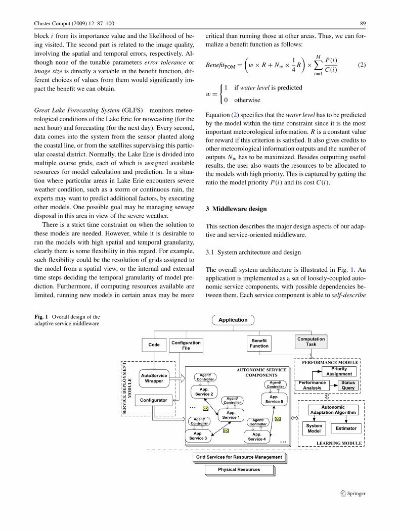
The overall system architecture is illustrated in Fig. 1. Anapplication is implemented as a set of loosely-coupled auto-nomic service components, with possible dependencies be-tween them. Each service component is able to self-describe

Fig. 1 Overall design of theadaptive service middleware

90 Cluster Comput (2009) 12: 87–100

its interface and self-optimize its contribution to the over-all processing. One service could invoke another servicefor certain functionality by communicating through SOAPmessages. In the VolumeRendering application fromthe previous section, the service for constructing a spatial-temporal tree would invoke a service specified in creatinga temporal tree, since each leaf node in the spatial treepresents its temporal information as a tree structure.

In order to facilitate the implementation of autonomicproperties for service components, our middleware includesa Service Deployment Module, a Performance Module anda Learning Module. When an application is submitted tothe system with its source code and the configuration file,the Service Deployment Module first decomposes the ap-plication and wraps it into autonomic service components.This is done by AutoServiceWrapper, which will be dis-cussed in the following subsection. Then, the configuratorextracts information such as dependencies between servicesand input/output specifications for service communication.The purpose of this module is to activate the applicationprocessing by executing its autonomic service components.

Each service component is programmed with adjustableservice parameters, such that the different choice of parame-ters could significantly impact the execution time, process-ing accuracy and the relative workload of different services.As we stated earlier, adapting these service parameters tomaximize the benefit function within the time constraints, isthe key function of the middleware. We implement an auto-nomic adaptation algorithm as part of the Learning Module.To be specific, it records the historical data and trains thesystem model and estimators during the normal processing.Details of the algorithm will be discussed in Sect. 4. ThePerformance Module cooperates with the Learning Moduleby analyzing the benefit function to decide the priority ofeach service component. This is important, as service pa-rameters from a service with higher priority could have amore significant impact on achieving our goal. Furthermore,when a particular event is detected, the Learning Module ap-plies the trained model and estimators to control parameteradaptation. At this time, the Performance Module iterativelyqueries the status of processing to avoid the violation of timeconstraints specified in the computation task.

3.2 AutoServiceWrapper: an autonomic service component

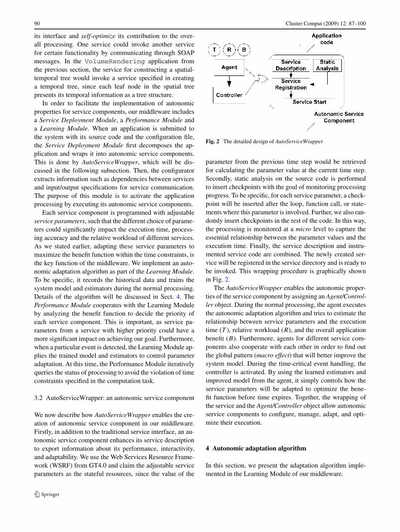
We now describe how AutoServiceWrapper enables the cre-ation of autonomic service component in our middleware.Firstly, in addition to the traditional service interface, an au-tonomic service component enhances its service descriptionto export information about its performance, interactivity,and adaptability. We use the Web Services Resource Frame-work (WSRF) from GT4.0 and claim the adjustable serviceparameters as the stateful resources, since the value of the

Fig. 2 The detailed design of AutoServiceWrapper

parameter from the previous time step would be retrievedfor calculating the parameter value at the current time step.Secondly, static analysis on the source code is performedto insert checkpoints with the goal of monitoring processingprogress. To be specific, for each service parameter, a check-point will be inserted after the loop, function call, or state-ments where this parameter is involved. Further, we also ran-domly insert checkpoints in the rest of the code. In this way,the processing is monitored at a micro level to capture theessential relationship between the parameter values and theexecution time. Finally, the service description and instru-mented service code are combined. The newly created ser-vice will be registered in the service directory and is ready tobe invoked. This wrapping procedure is graphically shownin Fig. 2.

The AutoServiceWrapper enables the autonomic proper-ties of the service component by assigning an Agent/Control-ler object. During the normal processing, the agent executesthe autonomic adaptation algorithm and tries to estimate therelationship between service parameters and the executiontime (T ), relative workload (R), and the overall applicationbenefit (B). Furthermore, agents for different service com-ponents also cooperate with each other in order to find outthe global pattern (macro effect) that will better improve thesystem model. During the time-critical event handling, thecontroller is activated. By using the learned estimators andimproved model from the agent, it simply controls how theservice parameters will be adapted to optimize the bene-fit function before time expires. Together, the wrapping ofthe service and the Agent/Controller object allow autonomicservice components to configure, manage, adapt, and opti-mize their execution.

4 Autonomic adaptation algorithm

In this section, we present the adaptation algorithm imple-mented in the Learning Module of our middleware.

Cluster Comput (2009) 12: 87–100 91

An application our middleware supports could compriseof a series of interacting services. Currently, each service isassumed to be deployed on a single node. The applicationinitiates one initial service, which then initiates, directly orindirectly, all other invoked services. The workload of suchinvoked service comprises of a series of function calls fromtheir invoking service. We assume that we have at least asmany nodes available as the services, and a separate nodecould be used for each service. In the future, we will con-sider the possibility that each service could be run on paral-lel platforms.

In such a case, we have three considerations. Obviously,we need to meet a time constraint, and second, we need tomaximize the benefit function. However, because of the in-teraction between the services, we need to consider anotherfactor, which is the relative workload of each service. Theoperating dynamics of a processor P executing one of theservices can be captured by the simple queuing model. Attime step k, λ(k) and β(k) denote the average arrival andprocessing rates associated with the processor P. The inputqueue size q(k) indicates the current workload on P, whichcan be calculated as:

q(k) = (λ(k) − β(k)) × Ts (3)

where Ts denotes the sampling period.

4.1 Algorithm overview

The intuition for our approach is as follows. The adaptationprocess in our framework corresponds to a typical optimalcontrol model [12]. The objective of optimal control theoryis to determine the control signals that will cause a processto satisfy the physical constraints, and at the same time, min-imize (or maximize) some performance criterion. The inputto our middleware is a number of services with dependen-cies involved. Each of them is programmed with adjustableservice parameters, as we had previously shown in our ex-amples from Sect. 2. When a particular event occurs, ouralgorithm controls the adaptation of the service parametersso as to optimize the benefit function, while satisfying thephysical constraints, which are the pre-defined time intervaland relative workload of the services. We assume that ourprocessing comprises a series of processing rounds, and val-ues of all service parameters can be modified between twoprocessing rounds.

Our approach is to first build a model for a particular ap-plication and estimate the effect of service parameters on ex-ecution time, relative workload of different services, and thebenefit function. Then, this model is deployed in the adapta-tion process of the application. In the VolumeRenderingapplication, the model specifies how error tolerance and im-age size would be changed based on their values from theprevious time step and the current action (increase/decrease

and by how much). However, the control problem of adjust-ing service parameters is a high-dimensional continuous-state task. For example, error tolerance is a real number be-tween 0 and 1. Then its control signal could be any real num-ber as long as the new value remains in the range. It is ex-tremely difficult to build an accurate model from the begin-ning. We propose an autonomic adaption algorithm that isable to quickly learn to perform well in the parameter adap-tion. Furthermore, the adaptation action taken at each ser-vice component will be converted to an effect in the overallsystem. Such global pattern could be the correlation betweenerror tolerance and image size in our example. Once it is de-tected, we could adapt both parameters in a non-conflictingway.

The algorithm falls into two phases, namely, a normalexecution phase and a event handling phase. In the normalexecution phase, we locally explore different values of ser-vice parameters to train the model and to estimate the re-lationships between service parameters and execution time,relative workload of different services, and the benefit func-tion. Once an event is detected and needs to be handled witha time constraint, the service parameters will be adapted us-ing the learned model.

4.2 Detailed problem formulation

In order to utilize the optimal control theory to model theadaptation process in our framework, we need to define asystem model. The variables we use in our model are listedin Table 1. In the VolumeRendering example, the vec-tor of state variables x(k) could be [error tolerance, imagesize]T . A possible control signal could be [0.005,−20]T ,which increases error tolerance by 0.005 and decreases im-age size by 20. Given the current values of these two para-meters, we can estimate the overall execution time and rel-ative workload of different services at time step k, whichis denoted as w(k) and q(k), respectively. Furthermore, thecorrective term v(k) may have to be applied because of thepossible correlation between error tolerance and image size.

State equation The system then is described by the lineartime-varying discrete-time state equation:

x(k) = Ax(k − 1) + Bu(k) + v(k) (4)

Table 1 Definitions for the system model

Variable Description

x(k) Adjustable service parameters

u(k) Increase/decrease to parameters

w(k) Estimated overall response time

v(k) Corrective term

q(k) Relative workload

92 Cluster Comput (2009) 12: 87–100

w(k) = w(k − 1) + f (x(k)) (5)

where k = 1, . . . , kN , representing the N processing rounds,and A and B are matrices with time-varying elements [12].They represent the time-varying system behavior and definethe linear relationship between a state variable x(k) in thecurrent state and the value from the previous state as well asits control signal. w(k) includes the time passed for the pre-vious k − 1 steps and the estimation f (x(k)) for the currentstep.

Performance measure The objective of the control prob-lem we are considering is to find the sequence u(1), . . . ,

u(N) to maximize the following performance criterion:

J = 1

2d1

(1

w0 − w(N)

)3

+N−1∑

k=1

[1

2d2

(B(x(k))

) − 1

2d3u2(k)

](6)

We denote w0 to be the pre-defined time constraint. Thefirst term here is designed to penalize the measure if thetime deadline is missed. The rest of the expression includesthe weighted benefit function estimation based on x(k) anda term for adaptation overhead. The goal is to maximizethe benefit function with minimum overhead of adaptation.Parameters d1, d2 and d3 can be chosen to give a rela-tive weight for meeting the time constraint, maximizing thebenefit, and minimizing the adaptation overhead. This is aquadratic function of the state x(k) and control input u(k),over the intermediate time steps specifies the trade-off be-tween the benefit function value, i.e., maximizing B(x(k)),and the corresponding application execution time w(N).Furthermore, u2(k) is the cost function that penalizes theadaptation overhead accumulated from N steps.

Physical constraints The formulated system model has thefollowing physical constraints.

C1: xmin ≤ x(k) ≤ xmax (7)

C2: q(k) ≤ Q (8)

The first constraint ensures that each service parametervaries within its own value range. The second constraint im-plies that the relative workload for each service componenthas to be below a certain threshold, as specified in the vec-tor Q. This vector is an input to the algorithm.

Discussion In this paper, we are proposing a linear time-varying discrete-time state equation to model the service pa-rameter adaptation. The rational is that first, the values of ad-justable parameters can only changed at checkpoints (time

steps) in the service processing, instead of being continu-ously tuned. Thus, the model should be based on discrete-time states. Furthermore, for simplicity, we use a linear re-lationship between the adjustable parameter value at twoconsecutive time steps in the proposed system model. How-ever, a general non-linear discrete-time first order dynamicalequation of the following form

x(k) = f k−1(x(k − 1), u(k − 1)) (9)

could also be used. The potential drawback could be thatthe learning phase may be longer now. Also, more drasticchanges to a parameter could result in either non-negligibleadaptation overhead, or the parameter could not be adaptedat an appropriate granularity. It is one of our future works toexplore such non-linear models.

4.3 Algorithm details

This subsection gives a detailed description of the adaptationalgorithm.

A challenge in our problem is to build an accurate modelto control the adaptation process in the event handling phase.Specifically, based on the system model discussed previ-ously, we have to decide u(k) given a certain state, the cor-rective term v(k), as well as estimating the relationships be-tween service parameters and execution time, relative work-load, and the benefit function.

Initial policy We apply a simple gradient-based method asthe initial control policy. To be specific, the control signalu(k) here is based on the difference of value in (6) betweenx(k) and x(k − 1), with d3 = 0. The performance functionused here includes the original benefit function associatedwith the application, and captures the penalty of missing thetime constraint. Given the parameter vector x(k − 1), wehave two possibilities. We are likely to miss the time con-straint, in which case, u(k) needs to decrease the penalty as-sociated with missing the time constraint. Alternatively, wemay not be missing the time constraint, and we can focuson increasing the benefit function. This simple initial policycould be written as:

u(k) = u(k − 1) − α � J ′ (10)

where, α is the learning rate and J ′ is the performance func-tion. Furthermore, we ignore v(k) in the initial policy.

The disadvantage of this initial policy is that it couldcause a large adaptation overhead. This overhead is depen-dent on the value of α. A large value would lead to a sit-uation where the adaptation is an iteration of increasing theservice parameters excessively and then decreasing them ex-cessively. A very small value would likely result in a veryslow convergence of the service parameters. We are also not

Cluster Comput (2009) 12: 87–100 93

considering the correlation between the different parame-ters, or formally, the term v(k). For example, if the correla-tion between error tolerance and image size is negative, weshould avoid increasing both the parameters simultaneously.

Control policy We use a reinforcement learning algorithm,i.e., Q-learning [25]. In order to satisfy the Markov property,we add in the workload for each processing round as the ran-domness factor in each state. Note that workload could varysignificantly with different processing rounds. However, wedo not take into account the impact of workload on parame-ter adaptation in this work. Given a state variable x(k), anaction u(k) should be taken if it has the highest probabilityto yield the maximum estimated action-value Q(x(k),u(k)).We compute Q(x(k),u(k)) based on the value of the perfor-mance function, as captured in (6) with d1 = d2 = 0.4 andd3 = 0.2. During the normal execution phase, we use Boltz-mann strategy [25] in Q-learning and conduct nearly pureexploration. For parameters with discontinued values, the al-gorithm simply tries each possible value for this service pa-rameter and records the choice with maximum benefit. How-ever, for continuous parameters, the search space for an ac-tion is infinite. We define a density function, π(u(k)|x(k)),to be the policy at time step k and draw n samples fromthe search pace as possible choices for u(k). The densityfunction specifies the probability of choosing an action u(k)

at the current state x(k). Furthermore, a higher probabilityto take the action u(k), the more performance gain it couldgenerate. Now, we define the control policy as follows:{

maxu(k) π(u(k)|x(k)) if x is continuous

maxu(k) TableLookUp(x(k), u(k)) otherwise

A kernel function [8] with � as the function parameters isused for the π(u(k)|x(k)). Q-learning updates � and thusimproves the control policy each processing round.

Besides deciding the control policy, we further make themodel more effective by taking potential global patternsinto account. The micro parameter adjustments cumulativelyproduce patterns we can notice at the macro level. One pos-sible global pattern to detect is the correlation between ser-vice parameters. By end of each processing rounds, agentsof different service components communicate with eachother and find out how different service parameters are cor-related. Thus, with the guidance of this relationship, wecould ignore the actions that will lead to conflicts. We denotethe correlation as v(k) in the system model. The other globalaspect relates to the relative workload. It assures a balancein the relative progress of different services. Recall from ourmiddleware design, the Performance Module assigns prior-ity to each service component. The service component withmore importance should be preserved to run with a balancedworkload. This is presented by constraint C2. A resource re-configuration will be activated if C2 is violated.

Estimating relationships We now discuss how we imple-ment estimators which are used during the normal execu-tion. Time: Recall that multiple checkpoints are inserted ineach service by the AutoServiceWrapper. During the normalexecution phase, the value of a service parameter xi and theexecution time of the block of code between two consecu-tive checkpoints, Cj and Ck , are recorded. Then the relation-

ship Tj,ki is regressed on xi using Recursive Least Square

(RLS) [24]. At the end of the learning phase, all Tj,ki will

be summed up to generate the relationship between the ex-ecution time of the service, denoted as Ti , and its serviceparameter xi . We further extend this relationship to be be-tween xi and the overall processing time of the applicationT , according to the dependencies of service components.This relationship is then used in (5). Therefore, in the eventhandling phase, we could estimate the time T at each check-point, given the current value of xi to see whether the timeconstraint will be violated or not. If so, xi should be adaptedaccordingly.

Relative workload Recall that

q(k) = (λ(k) − β(k)) × Ts

where Ts denotes the sampling period. At each service com-ponent, the relationship between β(k) and xi is regressedand used in (3). The algorithm checks the relative work-load vector q(k) to preserve a balanced workload on ser-vices with high priority. Otherwise, service parameters willbe adapted to assure better resource configuration.

Benefit In some cases, the relationship between a serviceparameter and the benefit function can be easily determinedfrom the expression of the benefit function. However, insome other cases, it may not be as simple. For example,BenefitVR is not directly expressed as a function of error tol-erance or image size. Instead, the values of both service pa-rameters could impact the number of blocks to be rendered,which is the first part in (1). Also, error tolerance could befurther decomposed to SE and TE, thus impacting the sec-ond part in the equation. We infer such relationships duringthe execution, by seeing how changing service parametersimpacts the parameters that appear in the expression for thebenefit function.

5 Experimental evaluation

This section presents results from a number of experimentswe conducted to evaluate the midleware and our autonomicadaptation algorithm. Specifically, we had the followinggoals in our experiments:

94 Cluster Comput (2009) 12: 87–100

• Demonstrate that the service parameters converge quicklywhile meeting the time constraint. Furthermore, the finalmethod we use turns out to be significantly more effectivethan a simple and intuitive approach, which is the initialpolicy we had described.

• Demonstrate that the overhead of adaptation is modest.For this, we compared the execution to the case where westart knowing the optimal parameter choices at the verybeginning. Our actual execution, on the other hand, needsto find values for these parameters at runtime.

• Demonstrate the overhead caused by learning is verysmall.

5.1 Experiment design

All our experiments were conducted in two Linux clusters,each of which consists of 64 computing nodes. Every nodehas 2 Opteron 250 (2.4 GHz) processors with 8 GB of mainmemory and 500 GB local disk space, interconnected withswitched 1 Gb/s Ethernet.

The experiments we report were conducted using two ap-plications, which we had described in Sect. 2. The first ap-plication is VolumeRendering. The procedure includes apreprocessing stage and a rendering stage, for which we cre-ated six services. Once the preprocessing is done, an imagewill be rendered for each time step. An interesting event wasdetected after certain time steps. Then, the detailed informa-tion would be generated in the particular area of the imagewhere the event occurred. The time-varying data we usedis a brick-of-byte (BOB) data set from Lawrence LivermoreNational Laboratory [17]. The details of VolumeRender-ing application are shown in Table 2.

There are three adjustable service parameters in this ap-plication. The wavelet coefficient, denoted as ω, is fromthe Compression Service. Both error tolerance and imagesize, denoted as τ and φ, are parameters in the Unit ImageProcessing Service. A large value of wavelet coefficient (ω)increases the time of compression and decompression andit varies between 4, 6, 8, 12, 16, and 20. Similarly, a smallvalue of error tolerance (τ ), or a big value of image size (φ)implies more communication as well as computation. Therange of them is [0,1] and (0,∞), respectively. The benefit

function is defined in (1). We found out that a smaller valueof τ yields more benefit from BenefitVR. The correlation be-tween φ and BenefitVR is positive. Furthermore, τ impactsBenefitVR more significantly than φ does.

The second application is referred to as POM. The res-olution of the computational grids covering the Lake Eriecould be varied from 2000 m×2000 m, 1000 m×1000 m to500 m×500 m. We created three services for POM. It startedwith the forecasting model running on top of the grids withthe resolution as 2000 m × 2000 m. Then, we simulated anevent occurring in a particular region of the lake. A finer-resolution grid will be activated to run the model for meteo-rological information predictions over this area. We list thedetails of the POM application in Table 2.

The tunable parameters in this application are the in-terval of internal time steps (Ti ), interval of external timesteps (Te), and grid resolution (θ ). They are from POMModel Services and the Grid Resolution Service, respec-tively. A large value of Ti or Te leads to less execution timefor the model. A small resolution means the calculation hasto be carried out in a more accurate way, thus resulting ina longer time interval. We had defined the benefit functionin (2). Through the experiments, we estimated that there isa relationship between BenefitPOM and Ti and Te. Further-more, the correlation is negative for Te and positive for Ti .

5.2 Autonomic adaptation algorithm for time constraint

Our first experiment demonstrated the benefits associatedwith the proposed adaptation algorithm implemented in ourmiddleware. We demonstrated the fast convergence of theservice parameters. Furthermore, this algorithm is more ef-fective compared to the adaptation under the initial policythat is discussed in Sect. 4.2. Both the VolumeRender-ing and POM applications were used for this experiment.

First, we show how the VolumeRendering applica-tion could benefit from the algorithm. In a specific computa-tion task, the user made the following requirements. Within20 minutes, the details of the image should be viewed at leastfrom view direction of 45◦, 90◦ and 135◦. Furthermore, theresolution of the image should be τ < 0.03 and the idealimage size for viewing is 256 × 256. We refer to the case

Table 2 Details of theVolumeRendering and POMapplications

Application Services Dataset

Preprocessing Rendering

Volume WSTP Tree Construction Service Unit Image Rendering Service

Rendering Temporal Tree Construction Service Decompression Service 6.5 GB

Compression Service Image Composition Service (30 time steps)

POM POM Model Service (2-D mode) POM Model Service (3-D mode)

Grid Resolution Service Linear Interpolation Service 21.0 GB

Cluster Comput (2009) 12: 87–100 95

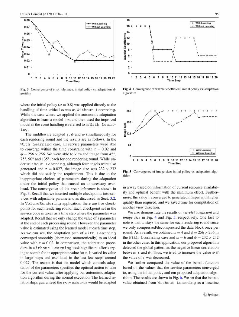
Fig. 3 Convergence of error tolerance: initial policy vs. adaptation al-gorithm

where the initial policy (α = 0.8) was applied directly to thehandling of time-critical events as Without Learning.While the case where we applied the autonomic adaptationalgorithm to learn a model first and then used the improvedmodel in the event handling is referred to as With Learn-ing.

The middleware adapted τ , φ and ω simultaneously foreach rendering round and the results are as follows. In theWith Learning case, all service parameters were ableto converge within the time constraint with τ = 0.02 andφ = 256 × 256. We were able to view the image from 45◦,75◦, 90◦ and 135◦, each for one rendering round. While un-der Without Learning, although four angels were alsogenerated and τ = 0.027, the image size was 232 × 232which did not satisfy the requirement. This is due to theinappropriate choices of parameters during the adaptationunder the initial policy that caused an unnecessary over-head. The convergence of the error tolerance is shown inFig. 3. Recall that we inserted multiple checkpoints into ser-vices with adjustable parameters, as discussed in Sect. 3.2.In VolumeRendering application, there are five check-points for each rendering round. Each checkpoint set in theservice code is taken as a time step where the parameter wasadapted. Recall that we only change the value of a parameterat the end of each processing round. However, the parametervalue is estimated using the learned model at each time step.As we can see, the adaptation path of With Learningconverged smoothly (decreased monotonically) to an idealvalue with τ = 0.02. In comparison, the adaptation proce-dure in Without Learning took significant efforts try-ing to search for an appropriate value for τ . It varied its valuein large steps and oscillated in the last few steps around0.027. The reason is that the model which controls adap-tation of the parameters specifies the optimal action to takefor the current value, after applying our autonomic adapta-tion algorithm during the normal execution. The learned re-lationships guaranteed the error tolerance would be adapted

Fig. 4 Convergence of wavelet coefficient: initial policy vs. adaptationalgorithm

Fig. 5 Convergence of image size: initial policy vs. adaptation algo-rithm

in a way based on information of current resource availabil-ity and optimal benefit with the minimum effort. Further-more, the value τ converged to generated images with higherquality than required, and we saved time for computation ofanother view direction.

We also demonstrate the results of wavelet coefficient andimage size in Fig. 4 and Fig. 5, respectively. One fact tonote is that ω stays the same for each rendering round sincewe only compressed/decompressed the data block once perround. As a result, we obtained ω = 4 and φ = 256 × 256 inthe With Learning case and ω = 6 and φ = 232 × 232in the other case. In this application, our proposed algorithmdetected the global pattern as the negative linear correlationbetween τ and φ. Thus, we tried to increase the value φ ifthe value of τ was decreased.

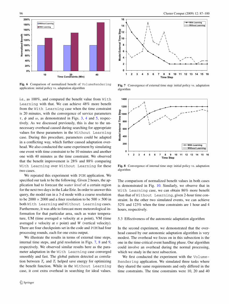
We further compared the value of the benefit functionbased on the values that the service parameters convergedto, using the initial policy and our proposed adaptation algo-rithm. The results are shown in Fig. 6. We set that the benefitvalue obtained from Without Learning as a baseline

96 Cluster Comput (2009) 12: 87–100

Fig. 6 Comparison of normalized benefit of VolumeRenderingapplication: initial policy vs. adaptation algorithm

i.e., as 100%, and compared the benefit value from WithLearning with that. We can achieve 48% more benefitfrom the With Learning case when the time constraintis 20 minutes, with the convergence of service parametersτ , φ and ω, as demonstrated in Figs. 3, 4 and 5, respec-tively. As we discussed previously, this is due to the un-necessary overhead caused during searching for appropriatevalues for these parameters in the Without Learningcase. During this procedure, parameters could be adaptedin a conflicting way, which further caused adaptation over-head. We also conducted the same experiment by simulatingone event with time constraint to be 10 minutes and anotherone with 40 minutes as the time constraint. We observedthat the benefit improvement is 28% and 88% comparingWith Learning over Without Learning for thesetwo cases.

We repeated this experiment with POM application. Wespecified our task to be the following. Given 2 hours, the ap-plication had to forecast the water level of a certain regionfor the next two days in the Lake Erie. In order to answer thisquery, the model ran in a 3-d mode with a coarse resolutionto be 2000 × 2000 and a finer resolution to be 500 × 500 inboth With Learning and Without Learning cases.Furthermore, it was able to forecast more meteorological in-formation for that particular area, such as water tempera-ture, UM (time averaged u velocity at u point), VM (timeaveraged v velocity at v point) and W (vertical velocity).There are four checkpoints set in the code and POM had fourprocessing rounds, each for one extra output.

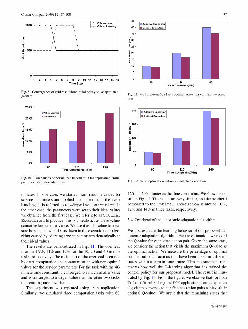
We illustrate the results in terms of external time steps,internal time steps, and grid resolution in Figs. 7, 8 and 9,respectively. We observed similar results here as the para-meter adaptation in the With Learning case convergedsmoothly and fast. The global pattern detected as correla-tion between Te and Ti helped save energy for optimizingthe benefit function. While in the Without Learningcase, it cost extra overhead in searching for ideal values.

Fig. 7 Convergence of external time step: initial policy vs. adaptationalgorithm

Fig. 8 Convergence of internal time step: initial policy vs. adaptationalgorithm

The comparison of normalized benefit values in both casesis demonstrated in Fig. 10. Similarly, we observe that inWith Learning case, we can obtain 86% more benefitthan that of Without Learning, given 2-hour time con-straint. In the other two simulated events, we can achieve52% and 123% when the time constraints are 1 hour and 4hours, respectively.

5.3 Effectiveness of the autonomic adaptation algorithm

In the second experiment, we demonstrated that the over-head caused by our autonomic adaptation algorithm is verymodest. The overhead we focus on in this subsection is theone in the time-critical event handling phase. Our algorithmcould involve an overhead during the normal processing,which we study in the next subsection.

We first conducted the experiment with the Volume-Rendering application. We simulated three tasks wherethey shared the same requirements and only differed in thetime constraints. The time constraints were 10, 20 and 40

Cluster Comput (2009) 12: 87–100 97

Fig. 9 Convergence of grid resolution: initial policy vs. adaptation al-gorithm

Fig. 10 Comparison of normalized benefit of POM application: initialpolicy vs. adaptation algorithm

minutes. In one case, we started from random values forservice parameters and applied our algorithm in the eventhandling. It is referred to as Adaptive Execution. Inthe other case, the parameters were set to their ideal valueswe obtained from the first case. We refer it to as OptimalExecution. In practice, this is unrealistic, as these valuescannot be known in advance. We use it as a baseline to mea-sure how much overall slowdown in the execution our algo-rithm caused by adapting service parameters dynamically totheir ideal values.

The results are demonstrated in Fig. 11. The overheadis around 9%, 11% and 12% for the 10, 20 and 40 minutetasks, respectively. The main part of the overhead is causedby extra computation and communication with non-optimalvalues for the service parameters. For the task with the 40-minute time constraint, τ converged to a much smaller valueand φ converged to a larger value than the other two tasks,thus causing more overhead.

The experiment was repeated using POM application.Similarly, we simulated three computation tasks with 60,

Fig. 11 VolumeRendering: optimal execution vs. adaptive execu-tion

Fig. 12 POM: optimal execution vs. adaptive execution

120 and 240 minutes as the time constraints. We show the re-sult in Fig. 12. The results are very similar, and the overheadcompared to the Optimal Execution is around 10%,12% and 14% in three tasks, respectively.

5.4 Overhead of the autonomic adaptation algorithm

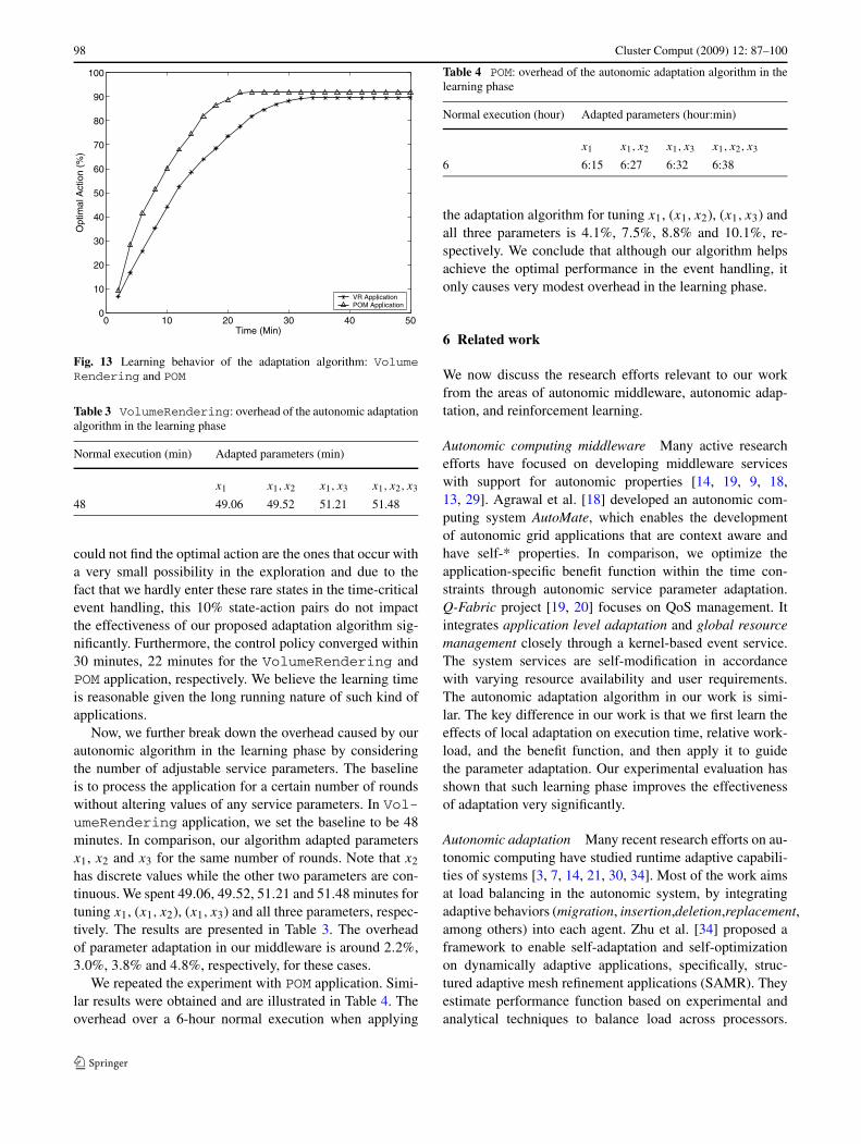
We first evaluate the learning behavior of our proposed au-tonomic adaptation algorithm. For the estimation, we recordthe Q-value for each state-action pair. Given the same state,we consider the action that yields the maximum Q-value asthe optimal action. We measure the percentage of optimalactions out of all actions that have been taken in differentstates within a certain time frame. This measurement rep-resents how well the Q-learning algorithm has trained thecontrol policy for our proposed model. The result is illus-trated by Fig. 13. From the figure, we observe that for bothVolumeRendering and POM applications, our adaptationalgorithm converge with 90% state-action pairs achieve theiroptimal Q-values. We argue that the remaining states that

98 Cluster Comput (2009) 12: 87–100

Fig. 13 Learning behavior of the adaptation algorithm: VolumeRendering and POM

Table 3 VolumeRendering: overhead of the autonomic adaptationalgorithm in the learning phase

Normal execution (min) Adapted parameters (min)

x1 x1, x2 x1, x3 x1, x2, x3

48 49.06 49.52 51.21 51.48

could not find the optimal action are the ones that occur witha very small possibility in the exploration and due to thefact that we hardly enter these rare states in the time-criticalevent handling, this 10% state-action pairs do not impactthe effectiveness of our proposed adaptation algorithm sig-nificantly. Furthermore, the control policy converged within30 minutes, 22 minutes for the VolumeRendering andPOM application, respectively. We believe the learning timeis reasonable given the long running nature of such kind ofapplications.

Now, we further break down the overhead caused by ourautonomic algorithm in the learning phase by consideringthe number of adjustable service parameters. The baselineis to process the application for a certain number of roundswithout altering values of any service parameters. In Vol-umeRendering application, we set the baseline to be 48minutes. In comparison, our algorithm adapted parametersx1, x2 and x3 for the same number of rounds. Note that x2

has discrete values while the other two parameters are con-tinuous. We spent 49.06, 49.52, 51.21 and 51.48 minutes fortuning x1, (x1, x2), (x1, x3) and all three parameters, respec-tively. The results are presented in Table 3. The overheadof parameter adaptation in our middleware is around 2.2%,3.0%, 3.8% and 4.8%, respectively, for these cases.

We repeated the experiment with POM application. Simi-lar results were obtained and are illustrated in Table 4. Theoverhead over a 6-hour normal execution when applying

Table 4 POM: overhead of the autonomic adaptation algorithm in thelearning phase

Normal execution (hour) Adapted parameters (hour:min)

x1 x1, x2 x1, x3 x1, x2, x3

6 6:15 6:27 6:32 6:38

the adaptation algorithm for tuning x1, (x1, x2), (x1, x3) andall three parameters is 4.1%, 7.5%, 8.8% and 10.1%, re-spectively. We conclude that although our algorithm helpsachieve the optimal performance in the event handling, itonly causes very modest overhead in the learning phase.

6 Related work

We now discuss the research efforts relevant to our workfrom the areas of autonomic middleware, autonomic adap-tation, and reinforcement learning.

Autonomic computing middleware Many active researchefforts have focused on developing middleware serviceswith support for autonomic properties [14, 19, 9, 18,13, 29]. Agrawal et al. [18] developed an autonomic com-puting system AutoMate, which enables the developmentof autonomic grid applications that are context aware andhave self-* properties. In comparison, we optimize theapplication-specific benefit function within the time con-straints through autonomic service parameter adaptation.Q-Fabric project [19, 20] focuses on QoS management. Itintegrates application level adaptation and global resourcemanagement closely through a kernel-based event service.The system services are self-modification in accordancewith varying resource availability and user requirements.The autonomic adaptation algorithm in our work is simi-lar. The key difference in our work is that we first learn theeffects of local adaptation on execution time, relative work-load, and the benefit function, and then apply it to guidethe parameter adaptation. Our experimental evaluation hasshown that such learning phase improves the effectivenessof adaptation very significantly.

Autonomic adaptation Many recent research efforts on au-tonomic computing have studied runtime adaptive capabili-ties of systems [3, 7, 14, 21, 30, 34]. Most of the work aimsat load balancing in the autonomic system, by integratingadaptive behaviors (migration, insertion,deletion,replacement,among others) into each agent. Zhu et al. [34] proposed aframework to enable self-adaptation and self-optimizationon dynamically adaptive applications, specifically, struc-tured adaptive mesh refinement applications (SAMR). Theyestimate performance function based on experimental andanalytical techniques to balance load across processors.

Cluster Comput (2009) 12: 87–100 99

Work presented by Lee et al. [14] applies an artificial im-mune system for autonomic adaptation. Once the immunesystem autonomously detects antigen, referring to networktraffic and resource availability, it adaptively performs a be-havior (antibody) to the sensed condition. Our work differsin the sense that our approach adjusts service parametersto impact the processing granularity. Furthermore, the goalof our autonomic adaptation algorithm focuses on the op-timization of the benefit function with time constraints, in-stead of load balancing.

Control theory is a well-established engineering field.The results from this area have recently been used to achieveadaptive behaviors in autonomic systems [1, 10, 32]. Wanget al. [32] applied Model Predictive Control (MPC) to man-age the power consumption of a computing cluster sub-ject to a dynamic workload while satisfying the specifiedQoS goals. They proposed a distributed cooperative controlframework where the optimization problem for the system isfirst decomposed into sub-problems, and solving each sub-problem achieves the overall performance objectives. Sim-ilarly, we also apply optimal control theory for the systemmodel. However, our work distinguishes in the followingways. Firstly, we do not assume that an accurate model isavailable for the system. Instead, we apply a reinforcementlearning algorithm to learn the model. Secondly, our frame-work involves low-overhead communication between agentsto detect global patterns, which further improves the modelto avoid conflict adaptations.

Reinforcement learning in autonomic computing An in-troduction of this field is available from [25]. Some appli-cations of these techniques are in robotics and control [4,15, 23], game playing [22, 26], and manufacturing [2, 16].Recently, RL has been used as a promising new approach fordeveloping autonomic systems [27, 28]. Tesauro et al. [28]applied RL to solve the problem of autonomic resource al-location, by taking the advantage of less built-in knowledge.

7 Conclusions

There are many applications where a timely response to animportant event is needed. Often such response can requiresignificant computation and possibly communication, and itcan be very challenging to complete it within the time-framethe response is needed. At the same time, there could beapplication-specific flexibility in the computation that maybe desired. This paper has presented the design, implemen-tation, and evaluation of a middleware that can support suchapplications. The main observations from our experimentsusing two real applications were as follows: When handlinga time-critical event, we were able to optimize the benefit

function within the pre-defined time constraint, with the pa-rameters converging quickly to their ideal values. Further-more, our algorithm was significantly more effective than asimple linear adaptation approach. The overhead of adapta-tion caused by our algorithm in time-critical event handlingis below 14%, when compared to an ideal or optimal execu-tion, which started with parameter values that were dynami-cally chosen by our algorithm. The overhead of the proposedalgorithm in the learning phase is only 5% for the volumerendering application and is around 10% for the Great Lakeforecasting application.

References

1. Bhat, V., Parashar, M., Liu, H., Khandekar, M., Kandasamy,N., Abdelwahed, S.: Enabling self-managing applications usingmodel-based online control strategies. In: Proceedings of the 3rdInternational Conference on Autonomic Computing (ICAC06),June 2005, pp. 15–24

2. Creighton, D.C., Nahavandi, S.: The application of a reinforce-ment learning agent to a multi-product manufacturing facility. In:Proceedings of the IEEE International Conference on IndustrialTechnology (ICIT02), pp. 1229–1234 (2002)

3. Cremene, M., Riveill, M., Martel, C.: Autonomic adaptationbased on service-context adequacy determination. Electron. NotesTheor. Comput. Sci. 189, 35–50 (2007)

4. Crites, R.H., Barto, A.G.: Improving elevator performance us-ing reinforcement learning. In: Proceedings of the Advances inNeural Information Processing Systems (NIPS 96), pp. 1017–1023 (1996)

5. Drebin, R.A., Carpenter, L., Hanrahan, P.: Volume rendering. In:Proceedings of the 15th Annual Conference on Computer Graph-ics and Interactive Techniques, pp. 65–74 (1988)

6. Foster, I., Kesselman, C., Nick, J.M., Tuecke, S.: The physiologyof the grid: An open grid services architecture for distributed sys-tems integration. Global Grid Forum, 189, Open Grid Service In-frastructure Working Group (2002)

7. Garlan, D., Chen, S., Huang, A., Schmerl, B., Steenkiste, P.: Rain-bow: Architecture-based self-adaptation with reusable infrastruc-ture. IEEE Comput. 37, 46–54 (2004)

8. Hertz, T., Hillel, A.B., Weinshall, D.: Learning a kernel func-tion for classification with small training samples. In: Proceed-ings of the 23rd International Conference on Machine Learning(ICML06), June 2006

9. Huang, G., Liu, T., Mei, H., Zheng, Z., Liu, Z., Fan, G.: Towardsautonomic computing middleware via reflection. In: Proceedingsof the 28th Annual International Computer Software and Applica-tions Conference(COMPSAC04), September 2004, pp. 135–140

10. Kandasamy, N., Abdelwahed, S., Hayes, J.P.: Self-optimization incomputer systems via on-line control: Application to power man-agement. In: Proceedings of the 1st International Conference onAutonomic Computing (ICAC04), June 2004, pp. 54–61

11. Kephart, J.O., Chess, D.M.: The vision of autonomic computing.IEEE Comput. 36, 41–50 (2003)

12. Kirk, D.E.: Optimal Control Theory: An Introduction. Prentice-Hall, Englewood Cliffs (1970)

13. Kumar, V., Cai, Z., Cooper, B.F., Eisenhauer, G., Schwan, K.,Mansour, M., Seshasayee, B., Widener, P.: Implementing diversemessaging models with self-managing properties using if low. In:Proceedings of the 3rd International Conference on AutonomicComputing (ICAC06), January 2006, pp. 243–252

100 Cluster Comput (2009) 12: 87–100

14. Lee, C., Suzuki, J.: An autonomic adaptation mechanism fordecentralized grid applications. In: Proceedings of the 3rdIEEE Consumer Communications and Networking Conference(CCNC06), January 2006, pp. 583–589

15. Mahadevan, S., Connell, J.: Automatic programming of behavior-based robots using reinforcement learning. In: Proceedings of theNinth National Conference on Artificial Intelligence (AAAI 91),pp. 768–773 (1991)

16. Mahadevan, S., Marchalleck, N., Das, T., Gosavi, A.: Self-improving factory simulation using continuous-time average-reward reinforcement learning. In: Proceedings of the 14th Inter-national Conference on Machine Learning (IMLC 97), pp. 202–210 (1997)

17. Mirin, A.A., Cohen, R.H., Curtis, B.C., Dannevik, W.P., Dimits,A.M., Duchauneau, M.A., Eliason, D.E., Schikore, D.R., Ander-son, S.E., Porter, D.H., Woodward, P.R., Shieh, L.J., White, S.W.:Very high resolution simulation of compressible turbulence on theIBM-SP system. In: Proceedings of ACM/IEEE SupercomputingConference (SC99), 1999

18. Parashar, M., Liu, H., Li, Z., Matossian, V., Schmidt, C., Zhang,G., Hariri, S.: Automate: Enabling autonomic grid applications.Cluster Comput. 9, 48–57 (2006)

19. Poellabauer, C., Abbasi, H., Schwan, K.: Cooperative run-timemanagement of adaptive applications and distributed resources.In: Proceedings of the 10th ACM International Conference onMultimedia, December 2002, pp. 402–411

20. Poellabauer, C., Schwan, K., Agarwal, S., Gavrilovska, A., Eisen-hauer, G., Pande, S., Pu, C., Wolf, M.: Service morphing: In-tegrated system- and application-level service adaptation in au-tonomic systems. In: Proceedings of the 5th Annual Interna-tional Workshop on Active Middleware Services (AMS03), June2003

21. Ruth, P., Junghwan, R., Dongyan, X., Kennell, R., Goasguen, S.:Autonomic live adaptation of virtual computational environmentsin a multi-domain infrastructure. In: Proceedings of the 3rd Inter-national Conference on Autonomic Computing (ICAC06), June2006, pp. 5–14

22. Samuel, A.L.: Some studies in machine learning using the gameof checkers. IBM J. Res. Dev. 3, 211–229 (1959)

23. Schaal, S., Atkeson, C.G.: Robot juggling: Implementation ofmemory-based learning. IEEE Control Syst. Mag. 14, 57–71(1994)

24. Scharf, L.L.: Statistical Signal Processing. Addison-Wesley,Reading (1991)

25. Sutton, R.S., Barto, A.G.: Reinforcement Learning: An Introduc-tion. MIT Press, Cambridge (1998)

26. Tesauro, G.: Temporal difference learning and td-gammon. Com-mun. ACM 38, 58–68 (1995)

27. Tesauro, G.: Reinforcement learning in autonomic computing: Amanifesto and case studies. IEEE Internet Comput. 11, 22–30(2007)

28. Tesauro, G., Jong, N.K., Das, R., Bennani, M.N.: A hybrid rein-forcement learning approach to autonomic resource allocation. In:Proceedings of the 3rd International Conference on AutonomicComputing (ICAC06), June 2005, pp. 65–73

29. Trumler, W., Petzold, J., Bagci, F., Ungerer, T.: Amon—autonomic middleware for ubiquitous environments applied to thesmart doorplate project. In: Proceedings of the 1st InternationalConference on Autonomic Computing (ICAC04), May 2004

30. Valetto, G., Kaiser, G., Phung, D.: A uniform programming ab-straction for effecting autonomic adaptations onto software sys-

tems. In: Proceedings of the 2nd International Conference on Au-tonomic Computing (ICAC05), June 2005, pp. 286–297

31. Wang, C., Garcia, A., Shen, H.W.: Interactive level-of-detail se-lection using image-based quality metric for large volume visual-ization. IEEE Trans. Vis. Comput. Graph. 13, 122–134 (2006)

32. Wang, M., Kandasamy, N., Guez, A., Kam, M.: Adaptive perfor-mance control of computing systems via distributed cooperativecontrol: Application to power management in computing clusters.In: Proceedings of the 3rd International Conference on AutonomicComputing (ICAC06), June 2006, pp. 165–174

33. Wang, C., Shen, H.W.: A framework for rendering large time-varying data using wavelet-based time-space partitioning (wtsp)tree. Technical report OSUCISRC-1/04-TR05, Department ofComputer and Information Science, Ohio State University (Jan-uary 2004)

34. Zhu, H., Parashar, M., Yang, J., Zhang, Y., Rao, S., Hariri, S.:Self-adapting, self-optimizing runtime management of grid appli-cations using pragma. In: Proceedings of the 17th IEEE Interna-tional Parallel and Distributed Processing Symposium (IPDPS03),April 2003

Qian Zhu received her B.E. degreein Computer Science from BeijingInformation and Technology Insti-tute, Beijing, China, in 2004. Cur-rently, she is a Ph.D. candidate ofthe Computer Science and Engi-neering Department at The OhioState University. Her research inter-ests include autonomic computing,grid computing and adaptive mid-dleware, with a focus on applyingmachine learning techniques for au-tonomic system management in dis-tributed environments. She is a stu-dent of IEEE.

Gagan Agrawal is a Professor ofComputer Science and Engineeringat the Ohio State University. He re-ceived his B.Tech. degree from In-dian Institute of Technology, Kan-pur, in 1991, and M.S. and Ph.D.degrees from University of Mary-land, College Park, in 1994 and1996, respectively. His research in-terests include parallel, distributedand data-intensive computing, com-pilers, data mining, and grid/cloudcomputing. He has published morethan 150 refereed papers in these ar-eas. He is a member of ACM and

IEEE Computer Society. He received a National Science FoundationCAREER award in 1998. He currently serves as an associate editorfor IEEE Transactions on Parallel and Distributed Computing. He alsoserved as a member of ACM dissertation award committee between1998 and 2003.