An adaptive freeway traffic state estimator

Automatica 45 (2009) 10–24

Contents lists available at ScienceDirect

Automatica

journal homepage: www.elsevier.com/locate/automatica

An adaptive freeway traffic state estimatorI

Yibing Wang a,∗, Markos Papageorgiou b,1, Albert Messmer c,2, Pierluigi Coppola d,3, Athina Tzimitsi b,1,Agostino Nuzzolo d,3a Institute of Transport Studies, Department of Civil Engineering, Monash University, VIC 3800, Australiab Dynamic Systems and Simulation Laboratory, Department of Production Engineering and Management, Technical University of Crete, 73100 Chania, Greecec Groebenseeweg 2, D-82402, Seeshaupt, Germanyd Department of Civil Engineering, ‘‘Tor Vergata’’ University of Rome, Rome, Italy

a r t i c l e i n f o

Article history:Received 6 May 2006Received in revised form7 November 2007Accepted 4 May 2008Available online 18 November 2008

Keywords:Stochastic macroscopic traffic flow modelExtended Kalman filterFreeway traffic state estimationJoint state and parameter estimationCongestionWeather conditionsTraffic incidentsDetector faultsTraffic incident alarmDetector fault alarm

a b s t r a c t

Real-data testing results of a real-time nonlinear freeway traffic state estimator are presented witha particular focus on its adaptive features. The pursued general approach to the real-time adaptiveestimation of complete traffic state in freeway stretches or networks is based on stochastic nonlinearmacroscopic traffic flow modeling and extended Kalman filtering. One major innovative aspect of theestimator is the real-time joint estimation of traffic flow variables (flows, mean speeds, and densities)and some important model parameters (free speed, critical density, and capacity), which leads to foursignificant features of the traffic state estimator: (i) avoidance of prior model calibration; (ii) automaticadaptation to changing external conditions (e.g. weather and lighting conditions, traffic composition,control measures); (iii) enabling of incident alarms; (iv) enabling of detector fault alarms. The purposeof the reported real-data testing is, first, to demonstrate feature (i) by investigating some basic propertiesof the estimator and, second, to explore some adaptive capabilities of the estimator that enable features(ii)–(iv). The achieved testing results are quite satisfactory and promising for further work and fieldapplications.

© 2008 Elsevier Ltd. All rights reserved.

1. Introduction

Real-time freeway traffic state estimation refers to estimatingtraffic flow variables (flows, space mean speeds, and densities)for a considered freeway stretch (see e.g. Wang and Papageorgiou(2005), Wang, Papageorgiou, and Messmer (2007)) or freewaynetwork (Wang, Papageorgiou, & Messmer, 2006; Wang et al.,in press) with an adequate time resolution (e.g. 5–10 s) andspatial resolution (e.g. 500 m or less) based on a limited amount

I This paper was not presented at any IFAC meeting. This paper wasrecommended for publication in revised form by Associate Editor Keum-Shik Hongunder the direction of Editor Mituhiko Araki.∗ Corresponding author. Tel.: +61 3 9905 9339; fax: +61 3 9905 4944.E-mail addresses: [email protected] (Y. Wang),

[email protected] (M. Papageorgiou), [email protected] (A. Messmer),[email protected] (P. Coppola), [email protected] (A. Tzimitsi),[email protected] (A. Nuzzolo).1 Tel.: +30 28210 37289; fax: +30 28210 37584.2 Tel.: +49 8801 95101; fax: +49 8801 95102.3 Tel.: +39 06 72597059; fax: +39 06 72597005.

0005-1098/$ – see front matter© 2008 Elsevier Ltd. All rights reserved.doi:10.1016/j.automatica.2008.05.019

of available measurement data from traffic detectors of varioustypes (e.g. inductive loops, video cameras, radar senors). It shouldbe emphasized that the number of traffic flow variables to beestimated may be much larger than the number of traffic flowvariables that are directly measured, and this is in fact theessential contribution of the traffic state estimation task. Real-timefreeway traffic state estimation is a fundamental task for freewaytraffic surveillance and control (Papamichail, Papageorgiou, &Wang, 2007) and has attracted a lot of investigation effortsin the past three decades. Related research proposed trafficstate estimation algorithms that were almost exclusively basedon macroscopic traffic flow modeling and (extended) Kalmanfiltering; see a concise review in Wang and Papageorgiou (2005).Following a similar avenue, this topic was recently investigatedfurther, and a general approach to the design of freeway trafficstate estimators was proposed (Wang & Papageorgiou, 2005).One distinct innovative aspect of this recent work is on-linemodel parameter estimation (Wang & Papageorgiou, 2005;Wang, Papageorgiou, & Messmer, 2003; 2006), i.e. real-timejoint estimation of all involved traffic flow variables and someimportant parameters (free speed, critical density, capacity) ofthe macroscopic traffic flow model employed by the traffic state

Y. Wang et al. / Automatica 45 (2009) 10–24 11

estimator. With the on-line model parameter estimation, foursignificant features may be achieved for the traffic state estimator:(i) Avoidance of off-line model calibration: When applying

macroscopic traffic flow modeling to a specific freeway stretch ornetwork, appropriate model parameter values are needed, whichare usually not precisely known beforehand and may indeed bedifferent from site to site. Therefore, before a traffic state estimatorcan be applied to a specific site, a tedious model calibrationprocedure usually has to be conducted off-line based on availabletraffic measurement data to identify the corresponding values ofthe model parameters (see e.g. Cremer and Papageorgiou (1981)and Papageorgiou, Blosseville, and Haj-Salem (1990)). However, ifthe model parameter values can also be properly estimated on-line (i.e. estimated simultaneously with the interested traffic flowvariables), the extra workload for off-line model calibration maybe avoided.(ii) Automatic adaptation to changing external conditions: For a

given site, the model parameter values may have to be changedsignificantly in real-time, in order for the employed model toreflect the impact of changing external conditions (weather andlighting conditions, percentage of trucks, variable speed limitsapplied, etc.) on the traffic flow characteristics. With fixedmodel parameter values (even if carefully pre-identified), a trafficstate estimator may not be able to work well under stronglychanging external conditions. However, if the estimator can adaptits model to the external condition changes via on-line modelparameter estimation using real-time traffic measurements, thecorresponding traffic situationsmay still be handled appropriately.(iii) Enabling of incident alarms: In case of incidents, the traffic

flow characteristics along the concerned freeway stretch maychange substantially; this may also be reflected in correspondinglydrastic changes of some model parameter values. With on-line model parameter estimation, such abrupt changes may beidentified in real time, and hence the incident occurrence may berecognized promptly, leading to corresponding incident alarms fortraffic operators.(iv) Enabling of detector fault alarms: In case of strong detector

malfunctions, the estimator has to adjust its model parametersradically in order for the local traffic state estimates to approachthe disfiguredmeasurements. Hence, the on-linemodel parameterestimates may also be used as an indicator for serious detectormalfunction.Recently a freeway traffic state estimator using on-line model

parameter estimation was developed and successfully tested insimulation (Wang & Papageorgiou, 2005; Wang et al., 2006),whereby the significance of on-line model parameter estimationfor proper traffic state estimation as well as the aforementionedestimator features were preliminarily demonstrated. In order todraw more reliable conclusions, the same traffic state estimatorwas also tested using real traffic measurement data collected fromthe A92 Freeway close to Munich, Germany, and the A3 Freewayin South Italy. Some representative testing results are presentedin this paper. It is important to mention that the average inter-detector spacing used in these recent tests is much larger thanthat reported inmost previousworks (seeWang and Papageorgiou(2005) for a review therein).The next section presents a stochastic nonlinear macroscopic

traffic flow model and a simple traffic measurement model,based on which the traffic state estimator is designed with theextended Kalman filtering. The A92 real-data testing in Germanyis subsequently reported so as, first, to demonstrate feature(i) by investigating some basic properties of the estimator and,second, to explore some adaptive capabilities of the estimatorthat enable features (ii) and (iii), particularly under changingexternal conditions and non-recurrent traffic incidents. The A3real-data testing in south Italy provides a large-scale field

application example for the designed traffic state estimator,which demonstrates feature (iv) as well as the overall adaptivecapabilities of the estimator. The main conclusions along withsome additional remarks on state estimation of nonlinear systemscorrupted with noise are provided in a final section.

2. Modeling and methodology

2.1. Stochastic macroscopic traffic flow model

A stochastic version of a nonlinear second-order validatedmacroscopic traffic flow model (Papageorgiou et al., 1990) isemployed in this paper to describe the dynamic behavior of trafficflow along a freeway stretch in terms of appropriate aggregatedtraffic flow variables. Any considered freeway stretch is sub-divided into a numberN of segmentswith lengths∆i, i = 1, . . . ,N ,while the time is discretized based on a time step T and the timeindex k = 0, 1, 2, . . .. The aggregated traffic flow variables aredefined in this discrete space–time frame as follows:

• Traffic density ρi(k) (in veh/km/lane) is the number of vehiclesin segment i at time instant kT , divided successively by thesegment length∆i and lane number λi.• Space mean speed vi(k) (in km/h) is the average speed of allvehicles included in segment i at time instant kT .• Traffic flow qi(k) (in veh/h) is the number of vehicles leavingsegment i during the time period [kT , (k+ 1)T ], divided by T .• On-ramp inflow ri(k) and off-ramp outflow si(k) (both in veh/h)at the segment i (if any).

It is shown in Papageorgiou et al. (1990) that the macroscopicmodel works pretty accurately with segment lengths ∆i in theorder of 500 m (or less) and model time step T in the order of10 s. Note that, for numerical stability reasons, T and ∆i must bechosen such that T < ∆i/vf , where vf denotes the free speed(to be explained in what follows). While subdividing a freewaystretch into segments, care should be taken that all geometricinhomogeneities or installed traffic detectors along the freewaystretch are located at the boundaries of the segments. Moreover,each segment is allowed to have at most one on-ramp or one off-ramp, preferably at the upstream boundary of the segment.For a segment i, the stochastic nonlinear difference equations of

the model are as follows:

ρi(k+ 1) = ρi(k)+T∆iλi[qi−1(k)− qi(k)+ ri(k)− si(k)] (1)

si(k) = βi(k) · qi−1(k) (2)

vi(k+ 1) = vi(k)+Tτ[V (ρi(k))− vi(k)]

+T∆ivi(k)[vi−1(k)− vi(k)]

−νTτ∆i

[ρi+1(k)− ρi(k)]ρi(k)+ κ

−δT∆iλi

ri(k)vi(k)ρi(k)+ κ

+ ξ vi (k), (3)

V (ρ) = vf exp[−1a

(ρ

ρcr

)a](4)

qi(k) = ρi(k) · vi(k) · λi + ξqi (k) (5)

where (1), (3)–(5) are the conservation equation, dynamic speedequation, stationary speed equation, and transport equation,respectively; βi(k) (dimensionless) denotes the exiting rate at theoff-ramp in segment i (if any); τ , ν, κ , δ, vf , ρcr , and a are modelparameters that may be given the same values for all segmentsof the considered freeway stretch; ξ vi (k) and ξ

qi (k) denote zero-

mean white noise acting on the empirical speed equation and theapproximate flow equation, respectively, to reflect the modeling

12 Y. Wang et al. / Automatica 45 (2009) 10–24

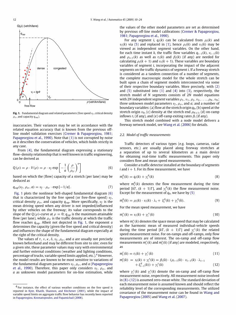
Fig. 1. Fundamental diagram and related parameters (free speed vf , critical densityρcr , and capacity qcap).

inaccuracies. Their variances may be set in accordance with therelated equation accuracy that is known from the previous off-line model validation exercises (Cremer & Papageorgiou, 1981;Papageorgiou et al., 1990). Note that (1) is not corrupted by noiseas it describes the conservation of vehicles, which holds strictly inany case.From (4), the fundamental diagram expressing a stationary

flow–density relationship that is well known in traffic engineering,can be derived as

Q (ρ) = ρ · V (ρ) = ρ · vf exp[−1a

(ρ

ρcr

)a](6)

based on which the (flow) capacity of a stretch (per lane) may bededuced as

qcap(vf , ρcr , a) = vf · ρcr · exp [−1/a] . (7)

Fig. 1 plots the nonlinear bell-shaped fundamental diagram (6)that is characterized by the free speed (or free-flow speed) vf ,critical density ρcr , and capacity qcap. More specifically, vf is themean driving speed when any driver is not impeded/influencedby other vehicles on the freeway; its value corresponds to theslope of the Q (ρ)-curve at ρ = 0; qcap is the maximum attainableflow (per lane), while ρcr is the traffic density at which the trafficflow reaches qcap. Albeit not depicted in Fig. 1, the exponent adetermines the capacity (given the free speed and critical density)and influences the shape of the fundamental diagram especially atthe right of the critical density.The values of τ , ν, κ , δ, vf , ρcr , and a are usually not precisely

known beforehand and may be different from site to site; even fora given site, these parameter values may vary with environmentaland further external conditions (weather and lighting conditions,percentage of trucks, variable speed limits applied, etc.).4 However,the model results are known to be most sensitive to variations ofthe fundamental diagram parameters vf , ρcr , and a (Papageorgiouet al., 1990). Therefore, this paper only considers vf , ρcr , anda as unknown model parameters for on-line estimation, while

4 For instance, the effect of various weather conditions on the free speed isreported in Kyte, Khatib, Shannon, and Kitchener (2001), while the impact ofvariable speed limits on aggregate traffic flow behavior has recently been reportedin Papageorgiou, Kosmatopoulos, and Papamichail (2008).

the values of the other model parameters are set as determinedby previous off-line model calibrations (Cremer & Papageorgiou,1981; Papageorgiou et al., 1990).For any segment i, qi(k) can be calculated from ρi(k) and

vi(k) via (5) and replaced in (1), hence ρi(k) and vi(k) may beviewed as independent segment variables. On the other hand,for each time instant k, the traffic flow variables qi−1(k), vi−1(k)and ρi+1(k) as well as ri(k) and βi(k) (if any) are needed forcalculating ρi(k + 1) and vi(k + 1). These variables are boundaryvariables of segment i, incorporating the impact of the adjacentsegments on the traffic dynamics of segment i. If a freeway stretchis considered as a tandem connection of a number of segments,the complete macroscopic model for the whole stretch can bebuilt upon a chain of segment models interconnected via someof their respective boundary variables. More precisely, with (2)and (5) substituted into (1) and (4) into (3), respectively, thestretch model of N segments consists of 2N model equationswith 2N independent segment variablesρ1, v1, ρ2, v2, . . . , ρN , vN ;three unknown model parameters vf , ρcr , and a; and a number ofboundary variables: (a) flowat the stretch origin q0, (b) speed at thestretch origin v0, (c) density at the stretch end ρN+1, (d) on-rampinflows ri (if any), and (e) off-ramp exiting rates βi (if any).This stretch model combined with a node model delivers a

freeway network model, see Wang et al. (2006) for details.

2.2. Model of traffic measurements

Traffic detectors of various types (e.g. loops, cameras, radarsensors, etc.) are usually placed along freeway stretches ata separation of up to several kilometres as a main devicefor obtaining real-time traffic measurements. This paper onlyconsiders flow and mean speed measurements.Consider a traffic detector installed at the boundary of segments

i and i+ 1. For its flow measurement, we have

mqi (k) = qi(k)+ γqi (k) (8)

where mqi (k) denotes the flow measurement during the timeperiod [kT , (k + 1)T ], and γ qi (k) the flow measurement noise.Except for the measurement of q0, we have by (5)

mqi (k) = ρi(k) · vi(k) · λi + ξqi (k)+ γ

qi (k). (9)

For the mean speed measurement, we have

mvi (k) = vi(k)+ γvi (k) (10)

wheremvi (k) denotes the spacemean speed thatmay be calculatedas the harmonic mean of measured individual-vehicle speedsduring the time period [kT , (k + 1)T ] and γ vi (k) the relatedspeed measurement noise. For on-ramps and off-ramps, only flowmeasurements are of interest. The on-ramp and off-ramp flowmeasurementsmri (k) andm

si (k) (if any) are modeled, respectively,

as

mri (k) = ri(k)+ γri (k) (11)

msi (k) = si(k)+ γsi (k) = βi(k) · (ρi−1(k) · vi−1(k) · λi−1

+ ξqi−1(k))+ γ

si (k) (12)

where γ ri (k) and γsi (k) denote the on-ramp and off-ramp flow

measurement noise, respectively. All measurement noise involvedin (8)–(12) is assumed zero-meanwhite. The standard deviation ofeach measurement noise is assumed known and should reflect thereliability level of the corresponding measurements. The utilizedcovariance of the measurement noise can be found in Wang andPapageorgiou (2005) and Wang et al. (2007).

Y. Wang et al. / Automatica 45 (2009) 10–24 13

2.3. State-space model and estimator design

For any freeway stretch, let vectors z, d, p, and ξ1 include,respectively, all segment variables, stretch boundary variables,unknown model parameters, and modeling noise. Then themacroscopic traffic flow model of a freeway stretch can beexpressed in a compact state-space form:

z(k+ 1) = h[z(k), d(k), p(k), ξ1(k)] (13)

where h is a nonlinear differential vector function correspondingto the 2N model equations previously mentioned. The utilizationof (13) requires the real-time availability of d(k) and (real-time)determination of p(k). However, some elements of d(k)may not bemeasured or even not measurable (Wang & Papageorgiou, 2005;Wang et al., 2006), while p(k) is normally unknown (or partiallyunknown). In order to overcome the obstacle of partially missingboundary measurements and unknown model parameters, model(13) may be extended using two random-walk equations:

d(k+ 1) = d(k)+ ξ2(k) (14)

p(k+ 1) = p(k)+ ξ3(k) (15)

where ξ2(k) and ξ3(k) are vectors of zero-meanwhite noise, whosecovariance matrices must be chosen so as to reflect typical timevariations of the boundary variables and model parameters.The combination of (13)–(15) leads to the following augmented

state-space model

x(k+ 1) = f[x(k), ξ(k)], (16)

where x =[zT dT pT

]T, ξ =

[ξT1 ξ

T2 ξT3

]T; the nonlinear

differentiable vector function f can be determined accordingly. Inthis paper, vector x is referred to as the traffic state.Consider a freeway stretch with traffic detectors installed at its

uppermost and lowermost boundaries, at some on/off-ramps, andperhaps also at some stretch-internal locations. The measurementmodel (8)–(12) can be written in a compact form as well:

y(k) = g[x(k), η(k)] (17)

where the output vector y consists of all available measurementsof flow and mean speed; g is a nonlinear differentiable vectorfunction; vector η is a function of state noise vector ξ andmeasurement noise vector γ . Eqs. (16) and (17) constitute acomplete freeway traffic dynamic system 6(x, y, ξ, η).Given real-time measurements y(k), the traffic state estimator

designed for 6(x, y, ξ, η) delivers state estimates:

x̂(k+ 1/k) = f[x̂(k/k− 1), 0] + K(k)[y(k)− g(x̂(k/k− 1), 0)].

Although some canonical forms other than 6(x, y, ξ, η) can alsobe constructed based on the presented traffic flow model andmeasurement model, 6(x, y, ξ, η) leads to a straightforward,general, and unique formulation of the traffic state estimatorfor any freeway stretch or network of any topology, size, andcharacteristics, with any suitable detector configuration (Wang &Papageorgiou, 2005; Wang et al., 2006).

3. Performance evaluation using real measurement data

3.1. A normal congestion case

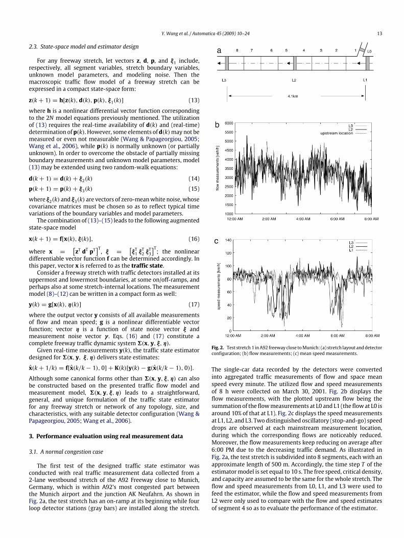
The first test of the designed traffic state estimator wasconducted with real traffic measurement data collected from a2-lane westbound stretch of the A92 Freeway close to Munich,Germany, which is within A92’s most congested part betweenthe Munich airport and the junction AK Neufahrn. As shown inFig. 2a, the test stretch has an on-ramp at its beginning while fourloop detector stations (gray bars) are installed along the stretch.

Fig. 2. Test stretch 1 inA92 freeway close toMunich: (a) stretch layout anddetectorconfiguration; (b) flow measurements; (c) mean speed measurements.

The single-car data recorded by the detectors were convertedinto aggregated traffic measurements of flow and space meanspeed every minute. The utilized flow and speed measurementsof 8 h were collected on March 30, 2001. Fig. 2b displays theflow measurements, with the plotted upstream flow being thesummation of the flowmeasurements at L0 and L1 (the flow at L0 isaround 10% of that at L1). Fig. 2c displays the speedmeasurementsat L1, L2, and L3. Two distinguished oscillatory (stop-and-go) speeddrops are observed at each mainstream measurement location,during which the corresponding flows are noticeably reduced.Moreover, the flow measurements keep reducing on average after6:00 PM due to the decreasing traffic demand. As illustrated inFig. 2a, the test stretch is subdivided into 8 segments, each with anapproximate length of 500 m. Accordingly, the time step T of theestimatormodel is set equal to 10 s. The free speed, critical density,and capacity are assumed to be the same for thewhole stretch. Theflow and speed measurements from L0, L1, and L3 were used tofeed the estimator, while the flow and speed measurements fromL2 were only used to compare with the flow and speed estimatesof segment 4 so as to evaluate the performance of the estimator.

14 Y. Wang et al. / Automatica 45 (2009) 10–24

The standard deviation (SD) values were set to be 100 veh/hand 10 km/h for the flow and speed modeling noise, respectively,and the same SD values were also used for the flow and speedmeasurement noise. In fact, the SD values of the modeling noisewere chosen so as to reflect the expected accuracy level of themodel equations (Cremer & Papageorgiou, 1981; Papageorgiouet al., 1990), while the SD values of the measurement noise werespecified according to the levels of typical measurement error ofloop detectors. Note that the SD values may need to be slightlytuned for specific sites. For all test examples reported in this paper,the utilized SD values vary between 50 and 200 veh/h for flows andbetween 5 and 10 km/h for speeds, and were always set constantfor a given site.The estimator’s performance was first examined without using

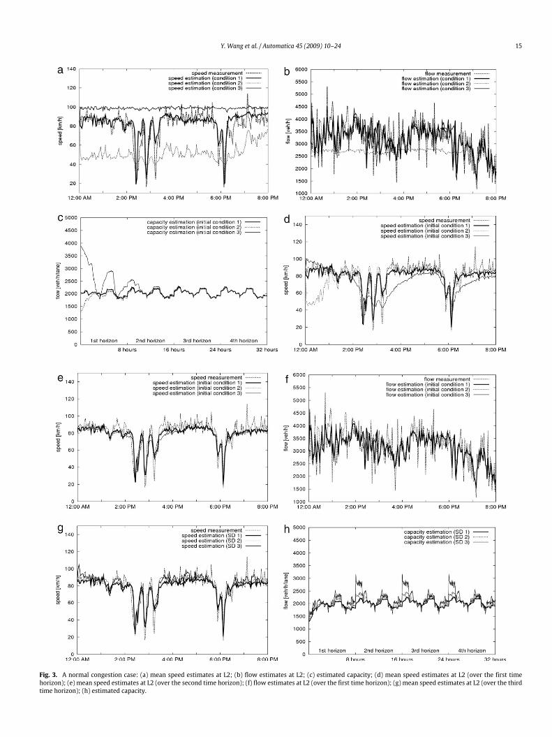
on-line model parameter estimation (i.e. keeping the parametersconstant at some pre-specified values over the investigationtime horizon). To this end, three groups of parameter valueswere considered, namely (95, 30, 2042), (85, 25, 1289), and(100, 50, 3894), each for the free speed (km/h), critical density(veh/km/lane), and capacity (veh/h/lane). These parameter groupsare referred to as parameter conditions 1, 2, and 3, respectively.The estimator was found capable of tracking the speed drops onlyunder parameter condition 1 as Fig. 3a presents, while the flowestimation was good under parameter conditions 1 and 3 (Fig. 3b).This demonstrates that:

(i) For a given test example, there exists (at least) one group ofnominal model parameter values, with which pretty accuratetraffic state estimates can be delivered by the estimator.Normally this specific group of parameter values can beobtained via off-line parameter identification.

(ii) If such nominalmodel parameter values are notwell identified(e.g. as in the case of parameter conditions 2 and 3), thenunacceptable traffic state estimation bias may result (evenunder free-flow conditions).

Next, the estimator is evaluated using on-linemodel parameterestimation, and the same parameter conditions 1–3 are usedas initial conditions. Note that the model parameters actuallyestimated are vf , ρcr , and a; however, since the flow capacityqcap can be calculated with vf , ρcr , and a through (7) and hasa more apparent physical interpretation than the exponent a,we will present in the rest of the paper the estimates of vf ,ρcr , and qcap. In order to check the dynamic evolution of thetraffic state estimates as well as the stability of the estimator, thetesting was conducted over a quadruple time horizon, wherebythe traffic scenario of the first time horizon (12:00 AM–8:00PM) was duplicated to the next three. Although the estimatesof the free speed, critical density, and capacity converge at theend of the second time horizon (see e.g. Fig. 3c for the capacityestimation), satisfactory speed estimates at L2 are delivered undereach initial condition already at the start of the second timehorizon (Fig. 3d and e), while satisfactory flow estimates at L2 areobtained even from the start of the first time horizon (Fig. 3f). It isimportant to mention that the shown ‘‘slow’’ convergence underinitial conditions 2 and 3, and hence the use of triple duplicateof the 8 h real data, are due to the ‘‘cold’’ start of the estimator,i.e. by use of an arbitrary initial matrix of the estimation covarianceand by use of the initial model parameter values that were setunrealistically far from normal values (just to demonstrate theestimator’s adaptive capability in achieving convergence evenwiththese extreme initial values). In contrast, under normal operationconditions (i.e. with a ‘‘warm’’ start incorporating some prior fieldknowledge of the model parameters), the estimator is seen, inthe subsequent sections with several demonstration examples(snowstorm, incident, and detector fault), to adapt the modelparameters promptly as appropriate. In fact, even for the current

test example with the ‘‘cold’’ start, the use of larger SD values forthemodel parameter noise ξ3 in (15) leads to faster convergence inthe estimation of both traffic flow variables andmodel parameters.In fact, a lower/higher SD of the noise for an estimated

model parameter is a ‘‘message’’ to the extended Kalman filterthat this parameter is less/more time-variant. More specifically,higher SDs are expected to lead to faster convergence of theparameter estimates but also more nervous behavior of theparameter estimates. The group of the SD values for ξ vf (k),ξρcr (k), and ξ a(k) (see (15)) utilized for the results in Fig. 3c–fis (0.1 veh/h, 0.02 veh/km/lane, 0.002), while two more groupsof SD values (0.2 veh/h, 0.04 veh/km/lane, 0.004) and (0.5 veh/h,0.1 veh/km/lane, 0.01) were also considered for a sensitivityinvestigation; these three groups of the SD values are referredto as SD 1, 2, and 3. The test demonstrates that the estimatesof traffic flow variables are little sensitive to the various groupsof the SD values (see e.g. Fig. 3g for the speed estimates at L2),although the corresponding parameter estimation trajectoriesmaybe different (see e.g. Fig. 3h for the capacity estimates). Note thatthe speed estimates in Fig. 3g are actually obtained over the thirdtime horizon under initial condition 2 (compare Fig. 3d, e, g),while virtually the same results as presented in Fig. 3g can bedelivered from the start of the third time horizon onwards underany initial condition (due to the aforementioned convergence).This low sensitivity property of the estimator with regard tovarious SD values used guarantees to a large extent the robustnessof the estimator and a very limited need for fine-tuning of the SDs.As shown in Fig. 3g and h, SD 1 seems to be most appropriateamong the three SD-groups, as it leads to minor variations ofthe model parameter estimates over time, while preserving theadaptive properties of the estimator as shown in Fig. 3c. Unlessspecifically mentioned, SD 1 (the nominal SD group) is consideredin the rest of the paper. The reader is also referred to Wang et al.(2007) formore results and interpretation in relation to the currenttest example.

3.2. A snowstorm case

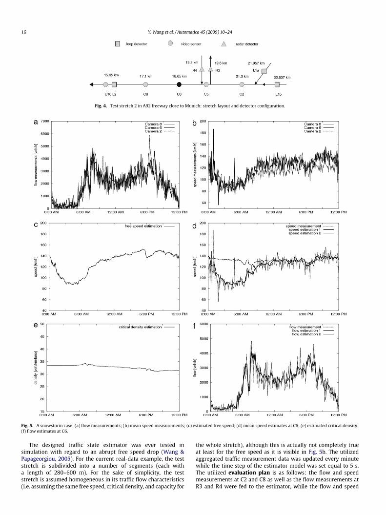
This testing was conducted in the same A92 Freeway in 2004.The involved freeway stretch is displayed in Fig. 4. In fact, thestretch shown in Fig. 2a is the downstream part of this one (fromthe on-ramp with R4 to the downstream end). Note that the A92Freewaywas extended from a two-lane freeway either direction toa three-lane one in 2003 (with its detector configuration changedas well). Accordingly, the traffic flow characteristics may also havechanged to an extent. It can be seen that five video detector stations(C2, C5, C6, C8, C10) and two loop detector stations (L1b and L2) areinstalled along the main stretch, while one loop detector station(L1a) is installed in a stretch merging into the main stretch, andtwo radar detector stations (R3 and R4) are installed respectivelyat the off-ramp and on-ramp. Fig. 5a and b display 24 h flow andspeed measurements collected at C8, C6, and C2 on February 11,2004. One may observe on the referred figures that the speedmeasurements decreased considerably from midnight until earlymorning, while the corresponding flowmeasurements kept steadyat very low values. Surprisingly, the speed measurements duringthis time period were even lower than those during the afternoonpeak period. Note that a similar observation was also deliveredby the other detectors placed along the stretch on the same day.With the help of the local transportation authority, it was foundout that a snowstorm was present in the area from the midnightuntil the morning of that day. It is not difficult to infer that thefree speed along the test stretch decreased substantially under thesnowstorm, which led to the observed speed decrease, despite avery low traffic flow.

Y. Wang et al. / Automatica 45 (2009) 10–24 15

Fig. 3. A normal congestion case: (a) mean speed estimates at L2; (b) flow estimates at L2; (c) estimated capacity; (d) mean speed estimates at L2 (over the first timehorizon); (e) mean speed estimates at L2 (over the second time horizon); (f) flow estimates at L2 (over the first time horizon); (g) mean speed estimates at L2 (over the thirdtime horizon); (h) estimated capacity.

16 Y. Wang et al. / Automatica 45 (2009) 10–24

Fig. 4. Test stretch 2 in A92 freeway close to Munich: stretch layout and detector configuration.

Fig. 5. A snowstorm case: (a) flow measurements; (b) mean speed measurements; (c) estimated free speed; (d) mean speed estimates at C6; (e) estimated critical density;(f) flow estimates at C6.

The designed traffic state estimator was ever tested insimulation with regard to an abrupt free speed drop (Wang &Papageorgiou, 2005). For the current real-data example, the teststretch is subdivided into a number of segments (each witha length of 280–600 m). For the sake of simplicity, the teststretch is assumed homogeneous in its traffic flow characteristics(i.e. assuming the same free speed, critical density, and capacity for

the whole stretch), although this is actually not completely trueat least for the free speed as it is visible in Fig. 5b. The utilizedaggregated traffic measurement data was updated every minutewhile the time step of the estimator model was set equal to 5 s.The utilized evaluation plan is as follows: the flow and speedmeasurements at C2 and C8 as well as the flow measurements atR3 and R4 were fed to the estimator, while the flow and speed

Y. Wang et al. / Automatica 45 (2009) 10–24 17

measurements at C6 were used only for evaluating the estimationresults. Typical testing results are presented in Fig. 5c–f. First, byactivating the on-linemodel parameter estimation, the estimator isable to identify and track in real time the free speed decrease underthe snowstorm (Fig. 5c) and deliver satisfactory speed estimates atC6 (‘‘estimation 1’’ in Fig. 5d). It is noted that the on-line estimatesof the critical density and exponent evolve steadily over time (seee.g. Fig. 5e for the critical density estimate); hence, in view of(7), the profile of the capacity estimation trajectory is very similarto that in Fig. 5c. Second, if the free speed is fixed at 140 km/h(i.e. forcing the estimator to ignore the snowstorm impact onthe free speed), the estimator fails to track the speed decrease(‘‘estimation 2’’ in Fig. 5d). However, in either case satisfactoryflow estimates at C6 can be obtained (Fig. 5f) as the conservationequation (1) does not seem to be strongly impacted by the modelmismatch.Due to a strong fog frommidnight until the morning of May 29,

2004, a speed limit of 80 km/h was applied in the A92 Freeway,which influenced the free speed and resulted in a clear speeddecrease during the fog hours. Similarly good traffic state estimateswere also obtained for that case (Wang, Papageorgiou, &Messmer,2005).

3.3. An incident case

3.3.1. Traffic congestion typesFrom a traffic state estimation point of view, freeway traffic

congestions can be classified as normal or abnormal. Given a free-way stretch, there are two types of normal congestions. Type 1occurs within the freeway stretch due to overload, e.g. at an exist-ing bottleneck, while Type 2 occurs sufficiently downstream of aconsidered stretch, creating an exogenous congestion shockwavethat propagates upstream and may eventually spill back into theconsidered stretch. The normal congestions of Type 1 are typicallyrecurrent congestions, while those of Type 2 may result from ei-ther recurrent congestions or traffic incidents. Under a normal con-gestion, the mean speeds upstream of the bottleneck (in the caseof Type 1) or along the stretch (in the case of Type 2) graduallydrop due to the shockwave propagation. For traffic state estima-tion under a normal congestion of Type 1, the macroscopic modelemployed by the estimator has sufficient knowledge regarding theexisting bottleneck, so that the congestion may be well tracked bythe estimator. A relevant simulation investigation was reported byWang et al. (2003, 2006). In the case of a normal congestion ofType 2, an upstream-moving shockwave reaches the downstreamboundary of the stretch and the speed and flow drops there aremeasured by the detectors installed at the boundary; thus, basedon the utilized model, the estimator is able to predict the prop-agation of the shockwave inside the stretch. A relevant real-datatesting was already presented in Section 3.1, where the congestionshockwave that was successfully tracked by the estimator, arrivedindeed from the downstream of L3.On the other hand, abnormal congestions are caused by

traffic incidents (e.g. collisions, disabled cars, etc.), and arecharacterized by abrupt and substantial real-time changes of theimpacted traffic flow characteristics, which may be reflected incorresponding changes of the model parameter values. Whena traffic incident occurs within a freeway stretch, usually anon-recurrent bottleneck is created temporarily around theincident location, and the local capacity, free speed, and criticaldensity decrease to an extent depending on the severity ofthe incident; moreover, the resulting congestion shockwavepropagates upstream. It is noted that a same incident-incurredcongestion can be an abnormal congestion for one stretch (ifthe incident occurs therein) but a normal congestion for anotherstretch (if the stretch is far upstream of the incident location). In

addition, if an incident occurs outside of a freeway stretch but quiteclose to its downstream boundary, the resulting congestion maystill have a clear impact on the local free speed, critical density,and capacity of that stretch.Under an incident-incurred abnormal congestion, (a) a flow

dropmay be observed at the detectors downstream of the incidentlocation, while the corresponding speed measurements may beseen to change only slightly; (b) both flow and speed drops maybe observed at the detectors upstream of the incident location (ifthese detectors are not located too far upstream). Then, due to thecontrast between the upstream and downstream measurements,the traffic state estimator is able to identify, via the on-line modelparameter estimation, the occurrence of an abnormal event (ofcourse, without knowing the exact reason). A real-data testingunder an abnormal congestion is reported below.

3.3.2. Incident alarmThis test was conducted in the same stretch as shown in Fig. 4,

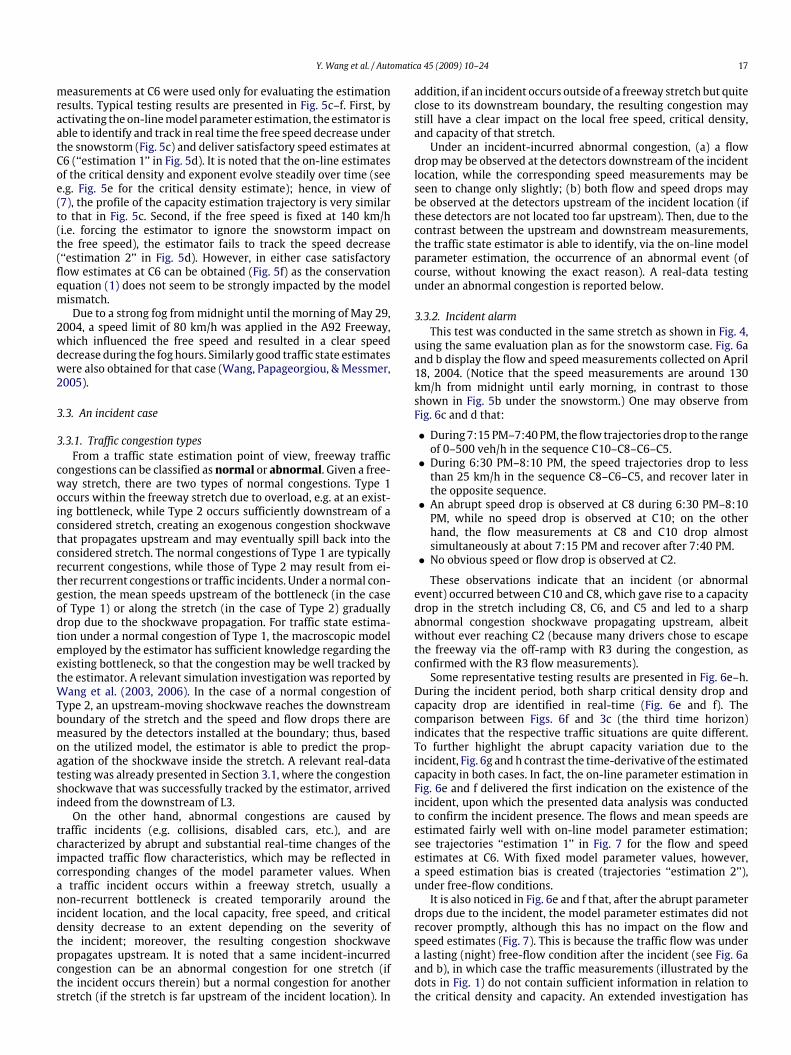
using the same evaluation plan as for the snowstorm case. Fig. 6aand b display the flow and speed measurements collected on April18, 2004. (Notice that the speed measurements are around 130km/h from midnight until early morning, in contrast to thoseshown in Fig. 5b under the snowstorm.) One may observe fromFig. 6c and d that:

• During 7:15 PM–7:40PM, the flow trajectories drop to the rangeof 0–500 veh/h in the sequence C10–C8–C6–C5.• During 6:30 PM–8:10 PM, the speed trajectories drop to lessthan 25 km/h in the sequence C8–C6–C5, and recover later inthe opposite sequence.• An abrupt speed drop is observed at C8 during 6:30 PM–8:10PM, while no speed drop is observed at C10; on the otherhand, the flow measurements at C8 and C10 drop almostsimultaneously at about 7:15 PM and recover after 7:40 PM.• No obvious speed or flow drop is observed at C2.

These observations indicate that an incident (or abnormalevent) occurred between C10 and C8, which gave rise to a capacitydrop in the stretch including C8, C6, and C5 and led to a sharpabnormal congestion shockwave propagating upstream, albeitwithout ever reaching C2 (because many drivers chose to escapethe freeway via the off-ramp with R3 during the congestion, asconfirmed with the R3 flow measurements).Some representative testing results are presented in Fig. 6e–h.

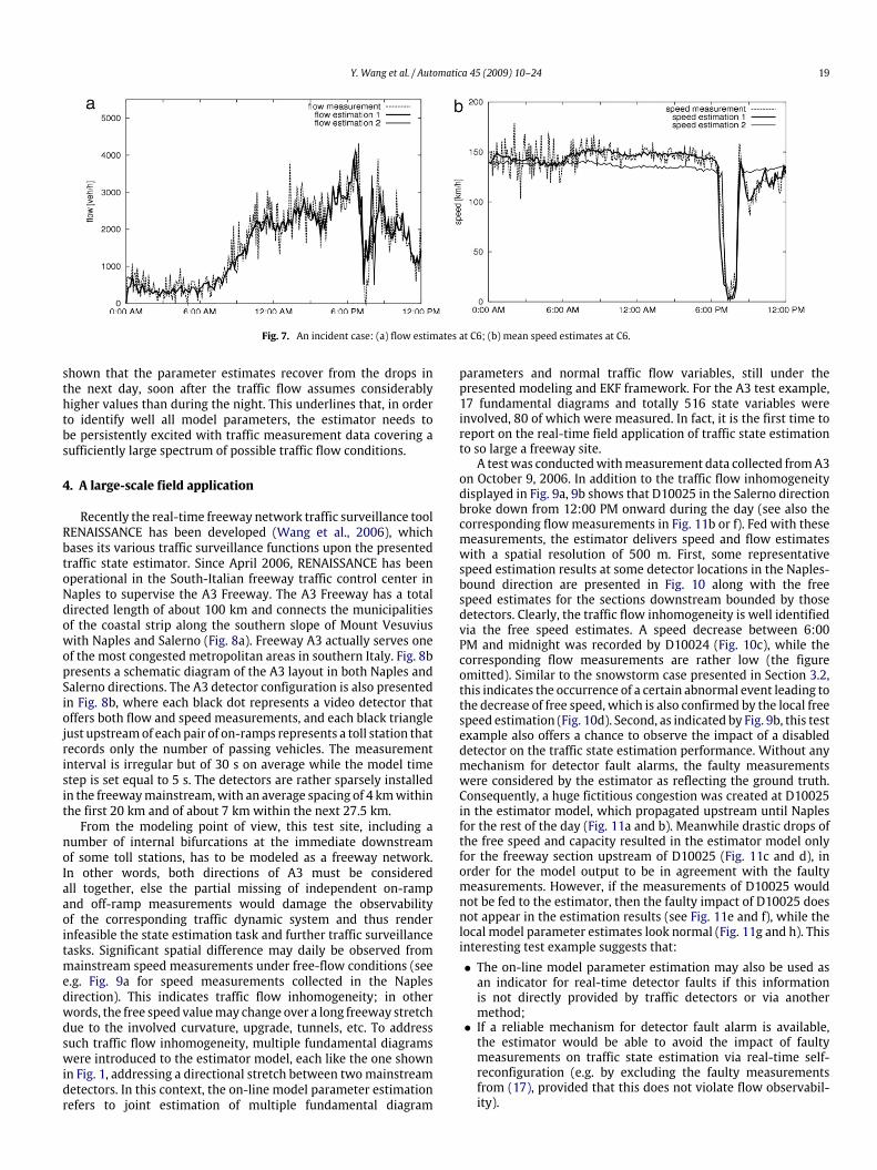
During the incident period, both sharp critical density drop andcapacity drop are identified in real-time (Fig. 6e and f). Thecomparison between Figs. 6f and 3c (the third time horizon)indicates that the respective traffic situations are quite different.To further highlight the abrupt capacity variation due to theincident, Fig. 6g and h contrast the time-derivative of the estimatedcapacity in both cases. In fact, the on-line parameter estimation inFig. 6e and f delivered the first indication on the existence of theincident, upon which the presented data analysis was conductedto confirm the incident presence. The flows and mean speeds areestimated fairly well with on-line model parameter estimation;see trajectories ‘‘estimation 1’’ in Fig. 7 for the flow and speedestimates at C6. With fixed model parameter values, however,a speed estimation bias is created (trajectories ‘‘estimation 2’’),under free-flow conditions.It is also noticed in Fig. 6e and f that, after the abrupt parameter

drops due to the incident, the model parameter estimates did notrecover promptly, although this has no impact on the flow andspeed estimates (Fig. 7). This is because the traffic flow was undera lasting (night) free-flow condition after the incident (see Fig. 6aand b), in which case the traffic measurements (illustrated by thedots in Fig. 1) do not contain sufficient information in relation tothe critical density and capacity. An extended investigation has

18 Y. Wang et al. / Automatica 45 (2009) 10–24

Fig. 6. An incident case: (a) flow measurements; (b) mean speed measurements; (c) zoom on the flow-drop period in (a); (d) zoom on the speed-drop period in (b);(e) estimated critical density; (f) estimated capacity; (g) and (h) estimated capacity derivative.

Y. Wang et al. / Automatica 45 (2009) 10–24 19

Fig. 7. An incident case: (a) flow estimates at C6; (b) mean speed estimates at C6.

shown that the parameter estimates recover from the drops inthe next day, soon after the traffic flow assumes considerablyhigher values than during the night. This underlines that, in orderto identify well all model parameters, the estimator needs tobe persistently excited with traffic measurement data covering asufficiently large spectrum of possible traffic flow conditions.

4. A large-scale field application

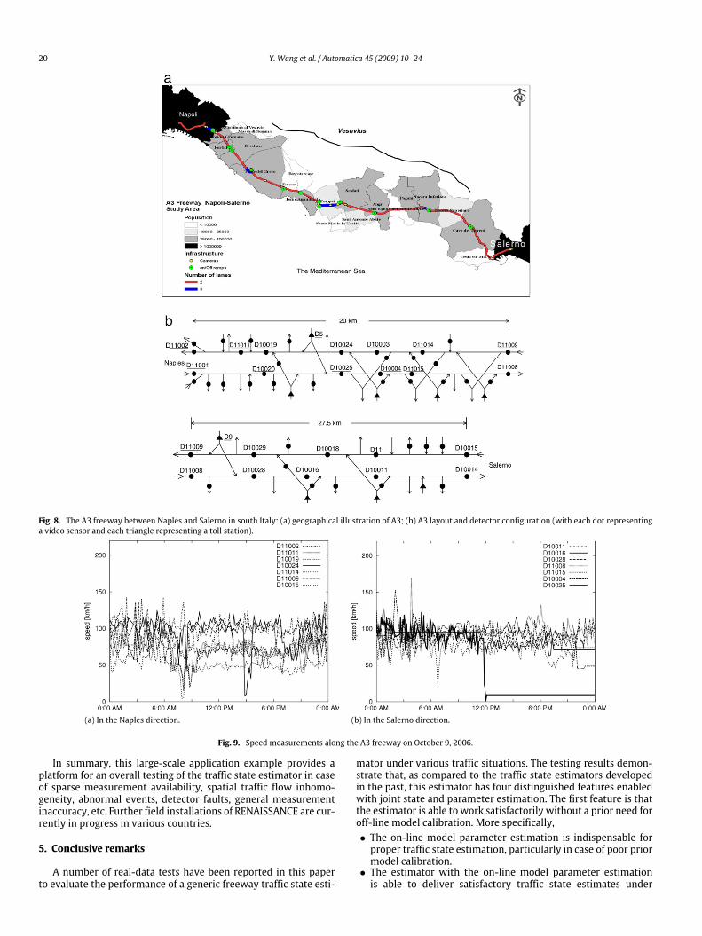
Recently the real-time freeway network traffic surveillance toolRENAISSANCE has been developed (Wang et al., 2006), whichbases its various traffic surveillance functions upon the presentedtraffic state estimator. Since April 2006, RENAISSANCE has beenoperational in the South-Italian freeway traffic control center inNaples to supervise the A3 Freeway. The A3 Freeway has a totaldirected length of about 100 km and connects the municipalitiesof the coastal strip along the southern slope of Mount Vesuviuswith Naples and Salerno (Fig. 8a). Freeway A3 actually serves oneof the most congested metropolitan areas in southern Italy. Fig. 8bpresents a schematic diagram of the A3 layout in both Naples andSalerno directions. The A3 detector configuration is also presentedin Fig. 8b, where each black dot represents a video detector thatoffers both flow and speed measurements, and each black trianglejust upstreamof each pair of on-ramps represents a toll station thatrecords only the number of passing vehicles. The measurementinterval is irregular but of 30 s on average while the model timestep is set equal to 5 s. The detectors are rather sparsely installedin the freewaymainstream,with an average spacing of 4 kmwithinthe first 20 km and of about 7 km within the next 27.5 km.From the modeling point of view, this test site, including a

number of internal bifurcations at the immediate downstreamof some toll stations, has to be modeled as a freeway network.In other words, both directions of A3 must be consideredall together, else the partial missing of independent on-rampand off-ramp measurements would damage the observabilityof the corresponding traffic dynamic system and thus renderinfeasible the state estimation task and further traffic surveillancetasks. Significant spatial difference may daily be observed frommainstream speed measurements under free-flow conditions (seee.g. Fig. 9a for speed measurements collected in the Naplesdirection). This indicates traffic flow inhomogeneity; in otherwords, the free speed valuemay change over a long freeway stretchdue to the involved curvature, upgrade, tunnels, etc. To addresssuch traffic flow inhomogeneity, multiple fundamental diagramswere introduced to the estimator model, each like the one shownin Fig. 1, addressing a directional stretch between twomainstreamdetectors. In this context, the on-line model parameter estimationrefers to joint estimation of multiple fundamental diagram

parameters and normal traffic flow variables, still under thepresented modeling and EKF framework. For the A3 test example,17 fundamental diagrams and totally 516 state variables wereinvolved, 80 of which were measured. In fact, it is the first time toreport on the real-time field application of traffic state estimationto so large a freeway site.A testwas conductedwithmeasurement data collected fromA3

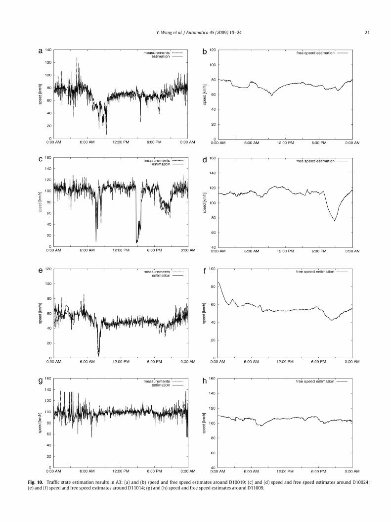
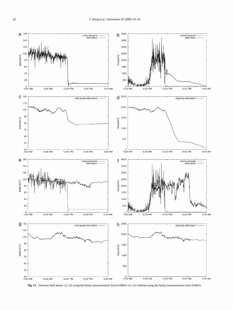
on October 9, 2006. In addition to the traffic flow inhomogeneitydisplayed in Fig. 9a, 9b shows that D10025 in the Salerno directionbroke down from 12:00 PM onward during the day (see also thecorresponding flowmeasurements in Fig. 11b or f). Fed with thesemeasurements, the estimator delivers speed and flow estimateswith a spatial resolution of 500 m. First, some representativespeed estimation results at some detector locations in the Naples-bound direction are presented in Fig. 10 along with the freespeed estimates for the sections downstream bounded by thosedetectors. Clearly, the traffic flow inhomogeneity is well identifiedvia the free speed estimates. A speed decrease between 6:00PM and midnight was recorded by D10024 (Fig. 10c), while thecorresponding flow measurements are rather low (the figureomitted). Similar to the snowstorm case presented in Section 3.2,this indicates the occurrence of a certain abnormal event leading tothe decrease of free speed, which is also confirmed by the local freespeed estimation (Fig. 10d). Second, as indicated by Fig. 9b, this testexample also offers a chance to observe the impact of a disableddetector on the traffic state estimation performance. Without anymechanism for detector fault alarms, the faulty measurementswere considered by the estimator as reflecting the ground truth.Consequently, a huge fictitious congestion was created at D10025in the estimator model, which propagated upstream until Naplesfor the rest of the day (Fig. 11a and b). Meanwhile drastic drops ofthe free speed and capacity resulted in the estimator model onlyfor the freeway section upstream of D10025 (Fig. 11c and d), inorder for the model output to be in agreement with the faultymeasurements. However, if the measurements of D10025 wouldnot be fed to the estimator, then the faulty impact of D10025 doesnot appear in the estimation results (see Fig. 11e and f), while thelocal model parameter estimates look normal (Fig. 11g and h). Thisinteresting test example suggests that:• The on-line model parameter estimation may also be used asan indicator for real-time detector faults if this informationis not directly provided by traffic detectors or via anothermethod;• If a reliable mechanism for detector fault alarm is available,the estimator would be able to avoid the impact of faultymeasurements on traffic state estimation via real-time self-reconfiguration (e.g. by excluding the faulty measurementsfrom (17), provided that this does not violate flow observabil-ity).

20 Y. Wang et al. / Automatica 45 (2009) 10–24

Fig. 8. The A3 freeway between Naples and Salerno in south Italy: (a) geographical illustration of A3; (b) A3 layout and detector configuration (with each dot representinga video sensor and each triangle representing a toll station).

(a) In the Naples direction. (b) In the Salerno direction.

Fig. 9. Speed measurements along the A3 freeway on October 9, 2006.

In summary, this large-scale application example provides aplatform for an overall testing of the traffic state estimator in caseof sparse measurement availability, spatial traffic flow inhomo-geneity, abnormal events, detector faults, general measurementinaccuracy, etc. Further field installations of RENAISSANCE are cur-rently in progress in various countries.

5. Conclusive remarks

A number of real-data tests have been reported in this paperto evaluate the performance of a generic freeway traffic state esti-

mator under various traffic situations. The testing results demon-strate that, as compared to the traffic state estimators developedin the past, this estimator has four distinguished features enabledwith joint state and parameter estimation. The first feature is thatthe estimator is able to work satisfactorily without a prior need foroff-line model calibration. More specifically,• The on-line model parameter estimation is indispensable forproper traffic state estimation, particularly in case of poor priormodel calibration.• The estimator with the on-line model parameter estimationis able to deliver satisfactory traffic state estimates under

Y. Wang et al. / Automatica 45 (2009) 10–24 21

Fig. 10. Traffic state estimation results in A3: (a) and (b) speed and free speed estimates around D10019; (c) and (d) speed and free speed estimates around D10024;(e) and (f) speed and free speed estimates around D11014; (g) and (h) speed and free speed estimates around D11009.

22 Y. Wang et al. / Automatica 45 (2009) 10–24

Fig. 11. Detector fault alarm: (a)–(d) using the faulty measurements from D10025; (e)–(h) without using the faulty measurements from D10025.

Y. Wang et al. / Automatica 45 (2009) 10–24 23

various traffic conditions (fluid, dense, congested), despite alarge average inter-detector spacing (4–7 km).• The estimator is little sensitive to the initial values of themodelparameters and traffic flow variables as well as to the relatedstandard deviations.The second feature is that the estimator can adapt itself

efficiently to the changes of weather conditions (like snow,fog, etc.), traffic composition (percentage of trucks), and controlmeasures (e.g. variable speed limits applied). The third featureis that under an incident-incurred abnormal congestion theestimator is able to issue an incident alarm promptly, whilehandling the traffic state estimation adequately. The fourth featureis that the estimator is capable of issuing alarms regarding obviousdetector faults. The real-time freeway network traffic surveillancetool RENAISSANCE (Wang et al., 2003, 2006) developed on thebasis of the reported adaptive traffic state estimator has beenoperational in the Naples freeway traffic control center in southItaly since April 2006 (Wang et al., in press), and will be soonimplemented in the Antwerp freeway traffic control center inBelgium and further freeway networks.The state estimation of nonlinear systems corrupted with noise

has been extensively considered in research and applications. Be-cause the optimal solution to this problem is infinite dimensional(see e.g. Kushner (1967)), a variety of approximate (or subopti-mal) approaches have been developed, amongwhich the extendedKalman filter (EKF) is probably most widely used (see e.g. Jazwin-sky (1970) and Sorenson (1985)). In the past three decades, nu-merous successful applications of the EKF have been reported inthe literature, but some intractable difficulties have also been en-countered. For example, the use of EKF was reported in some ap-plications to lead to biased estimates or even divergence, due tostepwise linearization (Julier &Uhlmann, 2004; Norgaard, Poulsen,& Ravn, 2000; Romanenko & Castro, 2004), inappropriate initialstate estimates (Glielmo, Setola, & Vasca, 1999; Ljung, 1979; Reif,Sonnemann, & Unbehauen, 1998), unknown covariance matricesof involved noise, or even the Gaussianity assumption of involvednoise (Arulampalam, Maskell, Gordon, & Clapp, 2002; Chen, Mor-ris, & Martin, 2005), etc. To address such problems, some othernonlinear filtering methods, especially unscented Kalman filter-ing (UKF) (Julier & Uhlmann, 2004) and particle filtering (PF) (Aru-lampalam et al., 2002), have been tested for a variety of stateestimation applications, gaining increasing popularity. Recentlysuch attempts towards traffic state estimation have also appeared(Antoniou, Ben-Akiva, & Koutsopoulos, 2007; Hegyi, Girimonte,Babuska, & De Schutter, 2006; Mihaylova, Boel, & Hegyi, 2007).The reported results demonstrate that the application of the EKF

to traffic state estimation is not strongly affected by the above-mentioned difficulties. In addition to the estimator’s adaptivefeatures shown, the estimator is seen little sensitive to the involvednoise statistics. More precisely, satisfactory functioning of thetraffic state estimator does not seem to require a prior knowledgeof noise characteristics (distribution or mean/covariance), andthis facilitates general applicability of the estimator. Nevertheless,comparable evaluations of EKF with UKF and PF for this significantapplication problem could indicate accuracy advantages of one oranother filtering approach.Besides accuracy, adaptiveness, and robustness, another con-

cern regarding traffic state estimation in relation to practical ap-plications is the computational real-time properties. In this aspectthe EKF-based approach is clearly superior to the UKF-based orPF-basedmethods. For instance, the presented EKF-estimator took11 h 34 min in a Pentium 4 personal computer (2.80 GHz, 1 GBRAM, Windows XP) to deal with 24 h measurement data (with ameasurement updating interval of 30 s to 1 min on average) fromthewhole A3 networkwith a total directed length of some 100 km.On the other hand, approaches may also be sought to improve thecomputational cost-effectiveness of alternative filtering methods(see e.g. Hegyi, Mihaylova, and Boel (2007)).

Acknowledgements

This research was partly supported by the European Commis-sion’s IST (Information Society Technologies) Program under theproject RHYTHM (IST-2000-29427). The authors thank Mr. O. Ern-hofer and Mr. Th. Heinrich from TRANSVER GmbH (Munich, Ger-many) for providing the utilized real traffic measurement datafrom the A92 Freeway close to Munich, Germany. The applicationof RENAISSANCE to the A3 Freeway in southern Italy was partlysupported by the Italian Ministry of University and Research un-der the project PON-SAM (No. 12897). The authors wish to thankthe projectmanagerMr. LuigiMassa from SAM (Società AutostradeMeridionali) in Naples, Italy. The completion of this paper was alsosupported in part by the Engineering New Staff Member ResearchFund and Engineering Small Grant (2008),MonashUniversity, Aus-tralia. All statements of this paper are under the sole responsi-bility of the authors and do not necessarily reflect the EuropeanCommission’s, the Italian Ministry of University and Research’s,Monash University’s, or other partners’ policies or views. Thispaper was partially presented at the 2005 IEEE Conference onIntelligent Transportation Systems and the 2006 TransportationResearch Board Annual Meeting. The authors wish to thank anony-mous reviewers for their critically helpful comments on a previousversion of the paper; in particular, the authors are much gratefulto one reviewer and the associate editor for their constructive sug-gestion that led to the adding of the large-scale field test example.

References

Antoniou, C., Ben-Akiva, M., & Koutsopoulos, H. N. (2007). Nonlinear Kalmanfiltering algorithms for on-line calibration of dynamic traffic assignmentmodels. IEEE Transactions on Intelligent Transportation Systems, 8, 661–670.

Arulampalam, M. S., Maskell, S., Gordon, N., & Clapp, T. (2002). A tutorial on particlefilters for online nonlinear/non-Gaussian Bayesian tracking. IEEE Transactionson Signal Processing , 50, 174–188.

Chen, T., Morris, J., & Martin, E. (2005). Particle filters for state and parameterestimation in batch processes. Journal of Process Control, 15, 665–673.

Cremer, M., & Papageorgiou, M. (1981). Parameter identification for a traffic flowmodel. Automatica, 17, 837–843.

Glielmo, L., Setola, R., & Vasca, F. (1999). An interlaced extended Kalman filter. IEEETransactions on Automatic Control, 44, 1546–1549.

Hegyi, A., Girimonte, D., Babuska, R., & De Schutter, B. (2006). A comparison offilter configurations for freeway traffic state estimation. In Proceedings of the9th international IEEE conference on intelligent transportation systems.

Hegyi, A., Mihaylova, L., & Boel, R. (2007). Parallelized particle filtering for freewaytraffic state tracking. In Proceedings of the 2007 European control conference.

Jazwinsky, A. H. (1970). Stochastic processes and filtering theory. NewYork: AcademicPress.

Julier, S. J., & Uhlmann, J. K. (2004). Unscented filtering and nonlinear estimation.Proceedings of IEEE, 92, 401–422.

Kyte, M., Khatib, Z., Shannon, P., & Kitchener, F. (2001). The effect of weather onfree flow speed. In Proceedings (CD-ROM) of transportation research board 80thannual meeting. Paper No. 01-3280.

Kushner, H. J. (1967). Dynamical equations for optimumnon-linear filtering. Journalof Differential Equations, 3, 179–190.

Ljung, L. (1979). Asymptotic behavior of the extended Kalman filter as a parameterestimator for linear systems. IEEE Transactions on Automatic Control, 24, 36–50.

Mihaylova, L., Boel, R., & Hegyi, A. (2007). Freeway traffic estimation within particlefiltering framework. Automatica, 43, 290–300.

Norgaard, M., Poulsen, N. K., & Ravn, O. (2000). New developments in stateestimation for nonlinear systems. Automatica, 36, 1627–1638.

Papageorgiou,M., Blosseville, J.-M., &Haj-Salem, H. (1990).Modelling and real-timecontrol of traffic flow on the southern part of Boulevard Périphérique in Paris-Part I: Modelling. Transportation Research A, 24, 345–359.

Papageorgiou, M., Kosmatopoulos, E., & Papamichail, I. (2008). Effects of variablespeed limits on motorway traffic flow. In Proceedings (CD-ROM) of the 87thtransportation research board meeting. Paper Number: 08-0781.

Papamichail, I., Papageorgiou, M., & Wang, Y. (2007). Motorway traffic surveillanceand control. European Journal of Control, 13, 297–319.

Reif, K., Sonnemann, F., & Unbehauen, R. (1998). An EKF-based nonlinear observerwith a prescribed degree of stability. Automatica, 34, 1119–1123.

Romanenko, A., & Castro, J. A. (2004). The unscented filter as an alternative to theEKF for nonlinear state estimation: A simulation case study. Computers andChemical Engineering , 28, 347–355.

Sorenson, H. W. (1985). Kalman filtering: Theory and application. New York: IEEEPress.

24 Y. Wang et al. / Automatica 45 (2009) 10–24

Wang, Y., Papageorgiou, M., & Messmer, A. 2003. Algorithms and preliminarytesting for traffic surveillance. Deliverable 3.2 for the Project RHYTHM (IST-2000-29427), report for the Information Society Technologies Office of the EuropeanCommission. Brussels, Belgium.

Wang, Y., & Papageorgiou, M. (2005). Real-time freeway traffic state estimationbased on extended Kalman filter: A general approach. Transportation ResearchB, 39, 141–167.

Wang, Y., Papageorgiou, M., & Messmer, A. 2005. An adaptive freeway traffic stateestimator and its real data testing, Part II: Adaptive capabilities. In Proceedingsof IEEE 8th international conference on intelligent transportation systems(pp. 537–542).

Wang, Y., Papageorgiou, M., & Messmer, A. (2006). RENAISSANCE — a unifiedmacroscopic model based approach to real-time freeway network trafficsurveillance. Transportation Research C , 14, 190–212.

Wang, Y., Papageorgiou, M, & Messmer, A. (2007). Real-time freeway traffic stateestimation based on extended Kalman filter: A case study. TransportationScience, 41, 167–181.

Wang, Y., Coppola, P., Messmer, A., Tzimitsi, A., Papageorgiou, M., & Nuzzolo, A.(2008). Real-time freeway network traffic surveillance: Large-scale field testingresults in southern Italy. IEEE Transactions on Intelligent Transportation Systems(in press).

Yibing Wang received the B.Sc. degree in Electronics andComputer Engineering from SichuanUniversity, China, theM. Eng. degree in Automatic Control Engineering fromChongqing University, China, and the Ph.D. degree in Con-trol Theory and Applications from Tsinghua University,China. He was with the Dynamic Systems and SimulationLaboratory, Department of Production Engineering andManagement, Technical University of Crete, Greece, wherehe was a Postdoctoral Researcher from 1999 to 2001 and aSenior Research Fellow from 2001 to 2007. He is currentlya Senior Lecturer with the Department of Civil Engineer-

ing, Monash University, Melbourne, Australia. His research interests include trafficflow modelling, freeway traffic surveillance, ramp metering, route guidance, urbantraffic signal control, vehicular infrastructure integration. He has published morethan 20 international journal papers and book chapters. He has extensive researchand development experience on intelligent transportation systems (ITS). From2000to 2007, he participated in several European projects on ITS and collaborated withtransportation research and practice professionals from Greece, Germany, UK, Bel-gium, Italy, and The Netherlands. Dr. Wang is a member of IEEE, an Associate Editorfor the IEEE Transactions on Intelligent Transportation Systems, the Book ReviewEditor of Transportation Research Part C: Emerging Technologies, an Associate Ed-itor for the International Journal of Vehicle Information and Communication Sys-tems, an Editorial BoardMember of The Open Transportation Journal. He was a vicechair of the International Program Committee of the 9th IEEE Annual Conference onIntelligent Transportation Systems (Toronto, 2006).

Markos Papageorgiou was born in Thessaloniki, Greece,in 1953. He received the Diplom-Ingenieur and Doktor-Ingenieur (honors) degrees in Electrical Engineering fromthe Technical University of Munich, Germany, in 1976 and1981, respectively. From 1976 to 1982 he was a Researchand Teaching Assistant at the Control Engineering Chair,Technical University of Munich. He was a Free Associatewith Dorsch Consult, Munich (1982–1988), and withInstitute National de Recherche sur les Transports etleur Sécurité (INRETS), Arcueil, France (1986–1988). From1988 to 1994 he was a Professor of Automation at

the Technical University of Munich. Since 1994 he has been a Professor atthe Technical University of Crete, Chania, Greece. He was a Visiting Professorat the Politecnico di Milano, Italy (1982), at the Ecole Nationale des Pontset Chaussées, Paris (1985–1987), and at MIT, Cambridge (1997, 2000); and aVisiting Scholar at the University of Minnesota (1991, 1993), the University ofSouthern California (1993) and the University of California, Berkeley (1993, 1997,2000).Dr. Papageorgiou is the author of the books Applications of Automatic Control

Concepts to Traffic Flow Modeling and Control (Springer, 1983) and Optimierung(Oldenbourg, 1991; 1996), the editor of the Concise Encyclopedia of Traffic andTransportation Systems (Pergamon Press, 1991), and co-author of Optimal Real-time Control of Sewer Networks (Springer, 2005) and the author or co-authorof some 300 technical papers. His research interests include automatic control

and optimization theory and applications to traffic and transportation systems,water systems and further areas. He is the Editor-in-Chief of TransportationResearch — Part C and an Associate Editor of IEEE Control Systems Society— Conference Editorial Board. He also served as an Associate Editor of IEEETransactions on Intelligent Transportation Systems and other journals. He wasChairman (1999–2005) and Vice-Chairman (1994–1999) of the IFAC TechnicalCommittee on Transportation Systems. He is a Fellow of IEEE. He receiveda DAAD scholarship (1971–1976), the 1983 Eugen–Hartmann award from theUnion of German Engineers (VDI), and a Fulbright Lecturing/Research Award(1997). He was the (first) recipient (2007) of the IEEE Outstanding ITS ResearchAward.

Albert Messmer received the Diplom-Ingenieur andDoktor-Ingenieur degrees in Electrical Engineering (witha focus on control engineering) from the TechnicalUniversity of Munich, Germany, in 1983 and 1994,respectively. Since 1994 he has been working as anindependent consultant. Since 1983 he has been engagedin modelling, simulation, optimization, and control ofmotorway networks and sewer systems. He has writtenmore than 30 technical papers on modelling and controlof water flow and freeway traffic.Dr. Messmer is a member of the Union of German

Engineers (VDI).

Pierluigi Coppola, born in Naples (Italy) in 1972, re-ceived the M. Eng. degree in Civil Engineering and thePh.D. in Road Infrastructures and Transportation Systemsfrom the ‘‘Federico II’’ University of Naples. He is cur-rently an assistant professor in Transportation planningat the Faculty of Engineering of ‘‘Tor Vergata’’ Univer-sity of Rome. His research interests include AdvancedTravellers Information Systems (ATIS) for road networksand Public Transportation systems, Land-Use/TransportInteractions (LUTI) models and network design meth-ods. He has published 30 journal papers and book

chapters. From 1998 to 2007 he has been involved in European and Na-tional research projects and practice professional on travel demand forecast-ing, network design and ITS, in Italy and in The Netherlands. Dr Coppola isa member of the Program Committee of the European Transport Conference(ETC).

Athina Tzimitsi was born in Naoussa, Greece, in 1974.She received the Diploma of Production Engineering andManagement and Master of Operational Research fromTechnical University of Crete, Greece, in 2005 and 2007,respectively. She was with the Dynamic Systems andSimulation Laboratory at Technical University of Cretefrom 2004 to 2008. She is now working in the privatesector.

Agostino Nuzzolo, born in Calvi (Italy) in 1949, is a fullprofessor of Transportation Planning at the Faculty of Engi-neering of ‘‘Tor Vergata’’ University of Rome. His researchwork is relative to the field of the theory of transporta-tion systems and its application in transportation analy-sis, modeling and planning. He is the author or co-authorof four books on the schedule-based approach to dynamictransportation networks and some 150 technical papersand book chapters. Prof. Nuzzolo is currently the presi-dent of the Italian Society of Lecturers of Transports (SIDT).He has been responsible of National and International re-

search projects on Traffic and Transportation Planning, Railway Services Pricing andDesign, Master Transport Plans, and on technical-economic feasibility studies oftransport infrastructures.