An adaptive choice of primal constraints for BDDC …etna.mcs.kent.edu/vol.45.2016/pp524-544.dir/pp524-544.pdfalso Section2.1. We note that algorithms using parallel sums for equivalence

Electronic Transactions on Numerical Analysis.Volume 45, pp. 524–544, 2016.Copyright c© 2016, Kent State University.ISSN 1068–9613.

ETNAKent State University

http://etna.math.kent.edu

AN ADAPTIVE CHOICE OF PRIMAL CONSTRAINTSFOR BDDC DOMAIN DECOMPOSITION ALGORITHMS∗

JUAN G. CALVO† AND OLOF B. WIDLUND‡

Abstract. An adaptive choice for primal spaces based on parallel sums is developed for BDDC deluxe methodsand elliptic problems in three dimensions. The primal space, which forms the global, coarse part of the domaindecomposition algorithm and which is always required for any competitive algorithm, is defined in terms of generalizedeigenvalue problems related to subdomain edges and faces; selected eigenvectors associated to the smallest eigenvaluesare used to enhance the primal spaces. This selection can be made automatic by using tolerance parameters specifiedfor the subdomain faces and edges. Numerical results verify the results and provide a comparison with primal spacescommonly used. They include results for cubic subdomains as well as subdomains obtained by a mesh partitioner.Different distributions for the coefficients are also considered with constant coefficients, highly random values, andchannel distributions.

Key words. elliptic problems, domain decomposition, BDDC deluxe preconditioners, adaptive primal constraints

AMS subject classifications. 65F08, 65N30, 65N35, 65N55

1. Introduction. There has recently been a considerable amount of activity in developingadaptive methods for the selection of primal constraints for BDDC algorithms and, in particular,for BDDC deluxe variants. The primal constraints of a BDDC or FETI–DP algorithm providethe global, coarse part of such a preconditioner, and they are of crucial importance for obtainingrapid convergence of these preconditioned conjugate gradient methods for the case of manysubdomains. When the primal constraints are chosen adaptively, we aim at selecting a primalspace which for a certain dimension of the coarse space provides the fastest rate of theconvergence for the iterative method. In the alternative, we can try to develop criteria whichwill guarantee that the condition number of the iteration stays below a given tolerance. Wenote that a fair comparison between different algorithms must also take into account the costof the set-up phase and the iterations to follow. So far a comparative study of these issues forthree dimensional problems, similar to the recent study [14] for problems in two dimensions,appears to be missing.

A particular inspiration for our own work has been a talk (see [7]) by Clark Dohrmann atDD21, the twenty-first international conference on domain decomposition methods held inRennes in June 2012. Dohrmann had then started a joint work with Clemens Pechstein; seealso [23]. Their work has recently resulted in a significant contribution to the theory; see [24].This rich paper also provides a historical context and many references to the literature.

Much of the earlier work for adaptive BDDC and FETI-DP iterative substructuringalgorithms, which has been supported by theory, has been confined to developing primalconstraints for equivalence classes related to two subdomain boundaries such as those for thesubdomain edges for problems defined on domains in the plane; see, in particular, the paperby Klawonn, Radtke, and Rheinbach [14]. In our context, the equivalence classes are sets offinite element nodes which belong to the boundaries of more than one subdomain with theequivalence relation defined by the sets of subdomain boundaries to which the nodes belong.In other words, two nodes on the interface Γ between the subdomains belong to the same

∗Received February 25, 2016. Accepted November 21, 2016. Published online on December 12, 2016. Recom-mended by Ulrich Langer. The work of J. G. C. was supported in part by the National Science Foundation GrantDMS-1216564. The work of O. B. W. was supported in part by the National Science Foundation Grants DMS-1216564and DMS-1522736.†CIMPA, Universidad de Costa Rica, San Jose, Costa Rica, 11501 ([email protected]).‡Courant Institute of Mathematical Sciences, 251 Mercer Street, New York, 10012, USA

([email protected]).

524



BDDC WITH ADAPTIVE PRIMAL SPACES 525

equivalence class if they belong to the same set of subdomain boundaries ∂Ωi. While it isimportant to further study the best way of handling all cases, the basic issues appear to be wellsettled when the equivalence classes all are defined by just two subdomain boundaries.

We note that this work is relevant for problems posed in H(div) even in three dimensions(3D) since the degrees of freedom on the interface between subdomains for Raviart-Thomasand Brezzi-Douglas-Marini elements are associated only with faces of the elements; see [22,29]. But for other elliptic problems in 3D, there is, except for quite special subdomainconfigurations, a need to develop algorithms and results for equivalence classes with three ormore subdomain boundaries.

There is early work by Mandel, Šístek, and Sousedík, who developed condition numberindicators; cf. [19, 20]. A firm theoretical foundation for these algorithms has now beendeveloped for problems in two dimensions and more recently for an enhanced variant and threedimensions; see [14] and [13], respectively. Talks by Clark Dohrmann and Axel Klawonnat DD23, the twenty-third international conference on domain decomposition methods heldin July 2015 on Jeju Island, Korea, have reported on recent progress. A talk by Hyea HyunKim in the same session on joint work with Eric Chung and Junxian Wang also has reportedconsiderable progress for a different kind of algorithm. Their main new algorithm for problemsin three dimensions is similar but not the same as ours; see further [12] and (3.6). The mainresult of this paper, which had been developed independently, has been reported on by thesecond author at the same DD23 mini-symposium.

This paper will focus on using parallel sums for general equivalence classes. The useof parallel sums for equivalence classes with two subdomain boundaries has proven verysuccessful in simplifying the formulas and arguments; see in particular Pechstein [23, 24] andalso Section 2.1. We note that algorithms using parallel sums for equivalence classes withmore than two subdomain boundaries have been quite successful in numerical experiments bySimone Scacchi and Stefano Zampini, reported in [5], for problems arising in isogeometricanalysis and also by Zampini [28] in a study of problems formulated in H(curl) based in parton [9].

We also note that we previously have attempted to design adaptive algorithms, whichresulted in quite complicated formulas and limited success. Among other complications, in oneof these approaches, the primal constraints then had to be extracted by using a QR factorizationof a matrix generated from several bases for spaces of prospective primal constraint vectorsrelated to pairs of Schur complements. We note that an alternative would be to carry out severalchanges of variables, thus enhancing the primal space in several steps, as is done in [11]. Seealso a discussion in [24].

In this paper, we will focus on low-order, nodal finite element approximations for scalarelliptic problems in three dimensions

(1.1) −∇ · (ρ(x)∇u) = f(x), x ∈ Ω, ρ(x) > 0,

resulting in a linear system of equations to be solved using BDDC domain decompositionalgorithms, in particular, its deluxe variant. We will always assume that the choice of boundaryconditions results in a positive definite, symmetric stiffness matrix. Future work is planned onwhat is known as the economic variant of the BDDC deluxe algorithm, (e-deluxe), cf. [9], andon linear elasticity including the almost incompressible case.

The outline of this paper is as follows: in Section 2, we briefly introduce the BDDCalgorithms. This is followed by a discussion of the case of equivalence classes with twosubdomain boundaries and a related generalized eigenvalue problem. The success of theadaptive algorithm in this case can be explained by examining the eigenvalues of a generalizedeigenvalue problem which is closely related to a face lemma. Such a lemma provides a standard



526 J. G. CALVO AND O. B. WIDLUND

technical tool in domain decomposition theory; see [26, Subsection 4.6.3]. Several numericalexperiments reported in Section 2.2 highlight the fact that a small number of primal constraintsoften can result in a very favorable bound.

We then, in Section 3, focus on the case of equivalence classes with three subdomainboundaries. This is the main part of our paper and is relevant, in particular, for contributions ofsubdomain edges to the values of a jump operator PD acting on the elements in a product spacerelated to the subdomains and the finite element space. We derive an upper bound of the squareof a norm based on a Schur complement and note that it has been known for over a decade thatsuch bounds provide an estimate of the condition number of the FETI–DP algorithm; see (2.1)and [16]. Given the close connection of the BDDC and FETI–DP algorithms, the bound forthat same jump operator is equally relevant for our work; see [18]. We find that the square ofthis norm of a subdomain edge contribution to PDw can be bounded from above in terms ofthree parallel sums of single Schur complements and sums of two others. We then attemptto find a common upper bound of these expressions in terms of the parallel sum of all therelevant Schur complements. This is not successful, and we instead work directly with theoperators obtained in the estimate of the jump operator and formulate a generalized eigenvalueproblem for each of the edges of the subdomains. We can then select a few eigenvectorsassociated with the smallest eigenvalues and generate a primal constraint from each of theseeigenvectors. These generalized eigenvalue problems are defined in terms of principal minorsof relevant Schur complements and Schur complements of these Schur complements associatedwith a minimal energy extension, e.g., from a subdomain edge of a three-dimensional finiteelement problem. We also provide a bound on the condition number in terms of the smallesteigenvalues for the subdomain faces and edges which have been left out when constructing theprimal space. We note that Kim et al. [12] have followed a quite similar path although theirupper bound for the norm of the jump operator differs from ours.

In a section that follows, we indicate how to extend our preconditioner and bounds toequivalence classes with four subdomain boundaries; no new ideas are required. Section 3 isconcluded by the definition of alternative generalized eigenvalue problems which has beenused with success in earlier work by Simone Scacchi and Stefano Zampini [5, 29]. So far thesealgorithms lack a theoretical foundation.

Our paper concludes, in Section 4, by demonstrating the performance of our algorithm ina series of numerical experiments using regular subdomains as well as subdomains generatedby a METIS mesh partitioner; see [10]. We demonstrate that we can obtain fast convergencefor problems with a quite irregular coefficient inside the subdomains. We also report onexperiments with two alternative algorithms based on other generalized eigenvalue problemsusing parallel sums and sums of the two sets of Schur complements; we have not been able toprovide a theoretical justification for these variants.

2. Equivalence classes and BDDC algorithms. This section begins with a short intro-duction to BDDC algorithms; for more details, see, e.g., [17]. For an introduction to its deluxevariant, see, e.g., [27].

BDDC algorithms are domain decomposition algorithms based on the decompositionof the domain Ω of an elliptic operator into non-overlapping subdomains Ωi, each oftenassociated with tens of thousands of degrees of freedom. The subdomain interface Γi of Ωidoes not cut through any elements and is defined by Γi := ∂Ωi \ ∂Ω. Its equivalence classesare associated with the subdomain faces, edges, and vertices of Γ :=

⋃i Γi, the interface of the

entire decomposition. Thus, for a problem in three dimensions, a subdomain face is associatedwith the degrees of freedom of the nodes belonging to the interior of the intersection of twoboundaries of two neighboring subdomains Ωi and Ωj and does not include any nodes on theboundary of the face. If such a set consists of several disjoint components, then each of them




will be classified as a face. Those of a subdomain edge are typically associated with a set ofnodes common to three or more subdomain boundaries, while the endpoints of the subdomainedges are the subdomain vertices which are associated with even more subdomains.

Given the stiffness matrix A(i) of the subdomain Ωi, we obtain a subdomain Schurcomplement S(i) by eliminating the interior variables, i.e., all those that do not belong to Γi.We will also work with principal minors of these Schur complements associated with faces Fand edges E denoting them by S(i)

FF and S(i)EE , respectively.

The interface space is divided into a primal subspace of functions which are continuousacross Γ and a complementary, dual subspace for which we will allow multiple values acrossthe interface during part of the iteration. In this study, all the subdomain vertex variables willalways belong to the primal set.

The BDDC and FETI–DP algorithms can be described in terms of three product spaces offinite element functions/vectors defined by their interface nodal values:

WΓ ⊂ WΓ ⊂WΓ.

WΓ is a product space of the spaces defined on the interfaces Γi without any continuityconstraints across the interface. Elements of WΓ have common values of the primal variablesbut allow multiple values of the dual variables while the elements of WΓ are continuous atall nodes on Γ. We will change variables, explicitly introducing the primal variables and acomplementary sets of dual variables in order to simplify the presentation; see, e.g., [17]. Aftereliminating the interior variables, we can then write the subdomain Schur complements as

S(i) =

[S

(i)∆∆ S

(i)∆Π

S(i)Π∆ S

(i)ΠΠ

].

We will partially subassemble the S(i), obtaining S, enforcing the continuity of the primalvariables only. Thus, we then work in WΓ. In each step of the iteration, we solve a linearsystem with the coefficient matrix S. In the alternative, we could also work with a linear systemwith a matrix obtained by partially subassembling the subdomain stiffness matrices A(i). Wenote that solving these linear systems will be considerably much faster than working with thefully assembled system provided that the dimension of the primal space is modest. At theend of each iteration, the approximate solution is made continuous at all nodal points of theinterface; continuity is restored by applying a weighted averaging operator ED, which mapsWΓ into WΓ.

In each iteration, we first compute the residual of the fully assembled Schur complementsystem. We then apply ETD to obtain a right-hand side for the partially subassembled linearsystem, solve this system, and then apply ED. This last step changes the values on Γ unlessthe iteration has converged and can result in non-zero residuals at nodes not on Γ. In a finalstep of each iteration step, we eliminate these residuals by solving a Dirichlet problem oneach of the subdomains. We always accelerate the iteration with the preconditioned conjugategradient algorithm.

2.1. BDDC deluxe. When designing a BDDC algorithm, we have to choose an effectiveset of primal constraints and also a good recipe for the averaging across the interface. Thispaper concerns the choice of the primal constraints while we will always use the deluxe recipein the construction of the averaging operator ED.

We note that in work on three-dimensional problems formulated in H(curl), it was foundthat traditional averaging recipes did not always work well; cf. [8, 9]. The same is true forproblems in H(div); see [22]. This occasional failure has its roots in the fact that there are two




sets of material parameters in these applications. The deluxe scaling that was then introducedhas also proven quite successful for a variety of other applications including isogeometricanalysis; cf. [5, 4]. For a survey, see [27].

A face component of the average operator ED across a subdomain face F ⊂ Γ commonto two subdomains Ωi and Ωj is defined in terms of the principal minors S(k)

FF of the matrixS(k), k = i, j. The deluxe averaging operator for F is then defined by

wF := (EDw)F :=(S

(i)FF + S

(j)FF

)−1 (S

(i)FFw

(i)F + S

(j)FFw

(j)F

).

Here, w(i)F is the restriction of w(i) to the face F, etc.

The action of (S(i)FF + S

(j)FF )−1 can be implemented by solving a Dirichlet problem on

Ωi ∪ F ∪ Ωj , where F is the face between the two subdomains. This can add significantlyto the cost. We can also compute the Schur complements, add them, and factor the sum. Wenote that if we would use the popular numerical factorization package MUMPS [1], we couldexploit that these Schur complements are provided when the subdomain matrices are factored.In an economic variant (e-deluxe), we replace this large domain by a thin domain built fromone or a few layers of elements next to the face, and this often results in very similar iterationcounts; see, e.g., [9]. The advantage of using the e-deluxe variant will depend considerably onthe software used in assembling a program; a discussion of these matters can be found in arecent paper on problems posed in H(div); see [22].

Deluxe averaging operators are also developed for subdomain edges and any other equiva-lence classes of interface variables, and the operator ED is assembled from all these compo-nents; see further Section 3. Our bound for this operator will be obtained from bounds for theindividual equivalence sets and will include factors that depend on the number of equivalenceclasses associated with the faces and edges of the individual subdomains; see Theorems 3.2and 3.4.

The core of any estimate for a BDDC algorithm is the norm of the averaging operator ED.By an algebraic argument known for FETI–DP since 2002, we know that

(2.1) κ(M−1BDDC S

)≤ ‖ED‖S ;

see [16]. Here, κ is the condition number of the iteration matrix, M−1BDDC denotes the BDDC

preconditioner, and S the fully assembled Schur complement of the problem.The analysis of any BDDC deluxe algorithm can be reduced to establishing bounds for

the individual subdomains. The analysis of traditional BDDC algorithms requires the use ofan extension theorem, cf. [15]; the deluxe version does not.

Instead of developing an estimate forED, we will work with PD := I−ED. Instead of es-timating the norm ofED, we will bound that of PD; we note that as proven in [24, Appendix A],the norm of these operators are the same. Thus, instead of estimating (RTF wF )TS(i)RTF wF ,we will work with the S(i)-norm of RTF (w

(i)F − wF ). Here, RF denotes the restriction to the

face F. By elementary algebra, we find that

w(i)F − wF =

(S

(i)FF + S

(j)FF

)−1

S(j)FF (w

(i)F − w

(j)F ).

More algebra gives, by using that S(i)FF := RFS

(i)RTF ,(RTF (w

(i)F − wF )

)TS(i)

(RTF (w

(i)F − wF )

)= (w

(i)F − w

(j)F )TS

(j)FF

(S

(i)FF + S

(j)FF

)−1

S(i)FF

(S

(i)FF + S

(j)FF

)−1

S(j)FF (w

(i)F − w

(j)F ).




Adding a similar contribution from Ωj , we obtain, following Clemens Pechstein, that therelevant expression of the energy is

(w(i)F − w

(j)F )TS

(i)FF

(S

(i)FF + S

(j)FF

)−1

S(j)FF (w

(i)F − w

(j)F )

= (w(i)F − w

(j)F )TS

(i)FF : S

(j)FF (w

(i)F − w

(j)F ).

The matrix of this positive definite, symmetric quadratic form is a parallel sum; we will usethe notation

A : B := A(A+B)−1B;

cf. [2]. We note that if A and B are positive definite, then A : B = (A−1 +B−1)−1. If A+Bis only positive semi-definite, then we can replace (A + B)−1 by (A + B)†, a generalizedinverse, without any complications. However, see [25] and Section 3 for a discussion of thecase of parallel sums of more than two positive semi-definite operators. We can also work withshifted, positive definite operators obtained by adding a small positive multiple of the identityoperator to the operators that are singular. This idea has worked well in our experiments; usinggeneralized inverses have produced results of quite similar quality.

In standard BDDC theory, the required estimate can then be obtained by using a facelemma, cf. [26, subsection 4.6.3], where such a result is established for constant coefficientsin each subdomain and for polyhedral subdomains. For an adaptive algorithm, this result isreplaced by the use of a generalized eigenvalue problem. Thus, we first solve the generalizedeigenvalue problem

(2.2) S(i)FF : S

(j)FFφ = λS

(i)FF : S

(j)FFφ.

Here,

S(i)FF := S

(i)FF − S

(i)TF ′F S

(i)−1F ′F ′ S

(i)F ′F ,

with S(i)F ′F ′ the principal minor of S(i) with respect to Γi \ F and S(i)

F ′F an off-diagonal blockof S(i). This Schur complement of a Schur complement represents the minimum norm exten-sion of any finite element function defined on F and will therefore provide a uniform bound forany extension of the values on F to the rest of Γi. In other words, w(i)T

F S(i)FFw

(i)F ≤ ai(w,w)

for any w that equals w(i)F on the face F. We note that the choice of S(i)

FF : S(j)FF as one of

the matrices of the generalized eigenvalue problem is fully motivated in the proof of [24,Lemma 5.24].

We note that the eigenvalue problem (2.2) can be replaced by an eigenvalue problem whichuses the inverses of the operators and that, following Zampini, we can extract the inverses ofall the matrices S(i)

FF from the inverse of S(i); the inverse of S(i)FF appears as a principal minor

of the inverse of S(i). The same trick can also be used to obtain all the matrices required foreigenvalue problems related to the subdomain edges which are developed in Section 3. Theinverses of S(i)

FF , etc., are computed via Cholesky factorizations. There are of course alsocosts in the set-up phase of the algorithm to solve a generalized eigenvalue problem for eachsubdomain face and each subdomain edge. We note that all these computations are local andcan be carried out in parallel. Detailed information on the relative cost of the set-up phase andthe iteration are provided for some large-scale parallel computations in [22].

Primal constraints are then generated by using the eigenvectors of a few of the smallesteigenvalues of (2.2) and making (S

(i)FF : S

(j)FF )(w

(i)F − w

(j)F ) orthogonal to these eigenvectors.




This orthogonality condition allows us to conclude that

wTF∆(S(i)FF : S

(j)FF )wF∆ ≤

1

λFtolwTF∆

(S

(i)FF : S

(j)FF

)wF∆

for any element wF∆ ∈ W∆, where λFtol is the smallest eigenvalue of the eigenvectors thathave not been chosen when we select the primal constraints. By using all the eigenvectorsas a new basis for the subspace associated with an individual subdomain face, we can easilyseparate primal and dual subspaces.

We note that the subdomain matrices A(i) are singular for interior subdomains and soare the Schur complements S(i)

FF . As it was previously pointed out, we can replace theinverses in the definition of the parallel sum, etc., by generalized inverses without any furthercomplications.

We now note that w(i)F − w

(j)F belongs to the dual space and that therefore

(w(i)F − w

(j)F )TS

(i)FF : S

(j)FF (w

(i)F − w

(j)F )

≤ 1

λFtol(w

(i)F − w

(j)F )T S

(i)FF : S

(j)FF (w

(i)F − w

(j)F ).

What remains is to estimate the expression on the right hand side by the energy attributedto the two subdomains Ωi and Ωj . To do so, we will use a formula for the parallel sum of twooperators; cf. [3, Theorem 9], see also [24, Corollary 5.11].

LEMMA 2.1. Let A and B be two symmetric, positive semi-definite matrices of the sameorder. Then, zTA : Bz = infz=x+y(xTAx+ yTBy).

Choosing x = w(i)F and y = −w(j)

F , we find that we have established the following result.LEMMA 2.2. Let λFtol be the smallest eigenvalue of (2.2) not chosen when selecting the

primal constraints for a subdomain face F . We then have

(2.3) ‖(PDw)|F ‖2S ≤1

λFtol(ai(w,w) + aj(w,w)) ,

where ai(·, ·) is the bilinear form associated with (1.1) obtained by restricting the integrationto Ωi, etc.

We note that a less precise version of formula (2.3) has previously been developed withthe factor 2

λFtol

; see, e.g., [14] as well as in the original version of this paper.

2.2. Convergence of eigenvalues. The success of this kind of algorithm is closely relatedto the rapid convergence of the eigenvalues of (2.2) to 1. Numerical experiments reportedin four plots illustrate a rapid decay of the eigenvalues of S(i)−1

FF (S(i)FF − S

(i)FF ) even for

problems with highly oscillatory coefficients; see Figure 2.1. The same can be said forsubdomains generated by the METIS mesh partitioner software; see Figure 2.2. This showsthat the eigenvalues of S(i)−1

FF S(i)FF approach 1 quite rapidly and that, except on a very small

subspace, the action of S(i)FF and S(i)

FF are virtually the same. Therefore the same can be saidof S(i)

FF : S(j)FF and S(i)

FF : S(j)FF . This fact is illustrated in four additional plots; see Figures 2.3

and 2.4.In the case of a random coefficient ρ(x), we use a uniform distribution to pick a number r

in the interval [−3, 3] and then assign the value 10r to ρ in individual elements.As a consequence of these findings, the eigenvalues of (2.2) converge to 1 quite rapidly

even for problems with large changes in the coefficients inside the subdomains. Therefore, wedo not need to expand the primal space very much.




0 50 100 150 200

10−15

10−10

10−5

100

ρ = 1.

0 50 100 150 200

10−15

10−10

10−5

100

Random ρ.

FIG. 2.1. Eigenvalues of S(i)−1FF (S

(i)FF − S

(i)FF ) for a face with 225 nodes of 3D problems with cubic subdomains.

0 10 20 30 40 50 60 70 80 90

10−10

10−5

100

ρ = 1.

0 10 20 30 40 50 60 70 80 90

10−15

10−10

10−5

100

Random ρ.

FIG. 2.2. Eigenvalues of S(i)−1FF (S

(i)FF − S

(i)FF ) for a face with 90 nodes of 3D problems with METIS

subdomains.

Figures 2.1 and 2.2 suggest that the operator S(i)−1FF (S

(i)FF − S

(i)FF ) is associated with a

compact operator. We can offer an explanation at least for the case with constant coefficients.We first recall that the trace class of H1(Ωi) is H1/2(∂Ωi). For a face F ⊂ ∂Ωi, the tracesemi-norm is defined by

(2.4) |u|2H1/2(F ) :=

∫F

∫F

|u(x)− u(y)|2

|x− y|3dSxdSy.

We obtain the H1/2(F )-norm by adding 1/HF ‖u‖2L2(F ), where HF is the diameter of F. We

find that the S(i)FF -norm is equivalent to the norm obtained by restricting (2.4) to the finite

element space; cf. [26, Lemma 4.6].It is also known that the H1/2(Γi)-norm of the minimal norm extension of any element

u ∈ H1/2(F ) is bounded uniformly by ‖u‖H1/2(F ). But it is also known that an extension by

zero even for H1/20 (F ), the closure of C∞0 (F ) in this norm, fails to be uniformly bounded.

The subspace for which the extension by zero is bounded is known as H1/200 (F ). A norm for

this subspace is given by

(2.5) ‖u‖2H

1/200 (F )

:= |u|2H1/2(F ) +

∫F

|u(x)|2

d(x)dSx,

where d(x) is the distance from x to ∂F. The formula (2.5) can be derived for any Lipschitz




0 50 100 150 2000

0.1

0.2

0.3

0.4

0.5

0.6

0.7

0.8

0.9

1

ρ = 1.

0 50 100 150 2000

0.1

0.2

0.3

0.4

0.5

0.6

0.7

0.8

0.9

1

Random ρ.

FIG. 2.3. Eigenvalues of S(i)FF : S

(j)FFφ = λS

(i)FF : S

(j)FFφ for a face with 225 nodes of 3D problems with

cubic subdomains.

0 10 20 30 40 50 60 70 80 900

0.1

0.2

0.3

0.4

0.5

0.6

0.7

0.8

0.9

1

ρ = 1.

0 10 20 30 40 50 60 70 80 900

0.1

0.2

0.3

0.4

0.5

0.6

0.7

0.8

0.9

1

Random ρ.

FIG. 2.4. Eigenvalues of S(i)FF : S

(j)FFφ = λS

(i)FF : S

(j)FFφ for a face with 90 nodes of 3D problems with

METIS subdomains.

region by considering the square of the H1/2(Γi)-norm of the extension of u(x) by zero ontoF ′ := Γi \ F ; see, e.g., [21].

A reflection of the fact that H1/200 is a true subspace of H1/2

0 (F ) is the well-known boundfor finite element spaces

‖uh‖2H1/200 (F )

≤ C (1 + log(Hi/hi))2 ‖uh‖2H1/2(F ),

which is known to be sharp; see [6, Lemma 4.2 and Remark 4.3] and also [26, Lemma 4.24]. Itis interesting to note that this estimate gives us an estimate of the smallest non-zero eigenvalueof (2.2); we can establish that in the special case considered, this eigenvalue is proportional to1/(1 + log(H/h))2; see also [26, Subsubsection 4.6.3].

The restriction of the new term∫F|u(x)|2d(x) dx to the finite element space gives a weighted

mass matrix which is spectrally equivalent to a diagonal matrix with elements varying inproportion to 1/d(x). This matrix is easily seen to be well approximated by a matrix of lowrank since the weight function 1/d(x) varies between values of 2/Hi and of 1/hi. It thenfollows that the matrix S(i)−1

FF (S(i)FF − S

(i)FF ) can be approximated well by a matrix of low

rank.

3. Equivalence classes with three subdomain boundaries. We begin this section byconsidering parallel sums of more than two operators. We will work with symmetric matriceswhich all are at least positive semi-definite. We recall that for a pair of symmetric, positive




definite matrices A and B, their parallel sum is given by A : B := A(A + B)−1B or(A−1 +B−1)−1. If A+B is singular, we can work with a generalized inverse.

For three positive definite matrices, we can define their parallel sum by

A : B : C := (A−1 +B−1 + C−1)−1,

with similar formulas for four or more matrices. A quite complicated formula for A : B : Cis given in [25] for the general case when some or all of the matrices might be only positivesemi-definite. It is also shown in [25, Theorem 3] that A : B : C = (A† +B† + C†)† if andonly if the three operators A,B, and C have the same range. In our context, this is not alwaysthe case since the matrix S(i)

EE defined below will be singular if Ωi is an interior subdomainwhile it will be non-singular if ∂Ωi intersects a part of ∂Ω where a Dirichlet condition isimposed. This issue can be avoided by making all operators non-singular by adding a smallpositive multiple of the identity to the singular operators.

As we previously have pointed out, our interest in working with parallel sums with morethan two operators is inspired by Scacchi’s and Zampini’s success in using parallel sums ofmore than two operators.

We will first focus on a case of an equivalence class common to three subdomain bound-aries as it arises for most subdomain edges in a three-dimensional finite element context if thesubdomains are generated using a mesh partitioner. We will use the notation S(i)

EE , S(j)EE , and

S(k)EE for the principal minors, of the degrees of freedom of an edge E, of the subdomain Schur

complements of the three subdomains that have this subdomain edge in common. The Schurcomplements of the Schur complements representing the minimal energy extensions to indi-vidual subdomains of given values on the subdomain edge E will be denoted by S(i)

EE , S(j)EE ,

etc., and are defined by

(3.1) S(i)EE := S

(i)EE − S

(i)TE′ES

(i)−1E′E′ S

(i)E′E , etc.

Here S(i)E′E′ is the principal minor of S(i) of Γi \ E, and S(i)

E′E is an off-diagonal block.We can now introduce the deluxe average over the edge E by

(3.2) wE :=(S

(i)EE + S

(j)EE + S

(k)EE

)−1 (S

(i)EEw

(i)E + S

(j)EEw

(j)E + S

(k)EEw

(k)E

).

We then establish that the contribution of the subdomain Ωi to the square of the norm of thecontribution of the edge to PDw = w − EDw is the square of the S(i)

EE-norm of(S

(i)EE + S

(j)EE + S

(k)EE

)−1 ((S

(j)EE + S

(k)EE

)w

(i)E − S

(j)EEw

(j)E − S

(k)EEw

(k)E

),

which can be estimated by the sum of

3w(i)TE

(S

(j)EE + S

(k)EE

)(S

(i)EE + S

(j)EE + S

(k)EE

)−1

S(i)EE

(S

(i)EE + S

(j)EE + S

(k)EE

)−1(S

(j)EE + S

(k)EE

)w

(i)E ,

3w(j)TE S

(j)EE

(S

(i)EE + S

(j)EE + S

(k)EE

)−1

S(i)EE

(S

(i)EE + S

(j)EE + S

(k)EE

)−1

S(j)EEw

(j)E ,

and

3w(k)TE S

(k)EE

(S

(i)EE + S

(j)EE + S

(k)EE

)−1

S(i)EE

(S

(i)EE + S

(j)EE + S

(k)EE

)−1

S(k)EEw

(k)E .

Here, we can replace w(i)E by the difference w(i)

E∆ between the original w(i)E and an appropriate

element in the primal space. The same shift is used to construct w(j)E∆ and w(k)

E∆.




The other two subdomains also contribute terms which can be obtained from the formulasabove by changing superscripts appropriately. The three terms that involve w(i)

E∆ are

3w(i)TE∆

(S

(j)EE + S

(k)EE

)(S

(i)EE + S

(j)EE + S

(k)EE

)−1

S(i)EE

(S

(i)EE + S

(j)EE + S

(k)EE

)−1(S

(j)EE + S

(k)EE

)w

(i)E∆,

3w(i)TE∆ S

(i)EE

(S

(i)EE + S

(j)EE + S

(k)EE

)−1

S(j)EE

(S

(i)EE + S

(j)EE + S

(k)EE

)−1

S(i)EEw

(i)E∆,

and

3w(i)TE∆ S

(i)EE

(S

(i)EE + S

(j)EE + S

(k)EE

)−1

S(k)EE

(S

(i)EE + S

(j)EE + S

(k)EE

)−1

S(i)EEw

(i)E∆.

By first adding the second and third terms and then usingA(A+B)−1B = B(A+B)−1A,we find that we can write the sum of these three terms as

3w(i)TE∆ S

(i)EE :

(S

(j)EE + S

(k)EE

)w

(i)E∆.

There are also two additional terms representing the squares of certain norms ofw(j)E∆ andw(k)

E∆.They are obtained by appropriately permuting the superscripts.

This formula represents a simplification of what was worked out in a joint paper withBeirão da Veiga et al. [4] and also in the development of the theory in a more recent paperwith Dohrmann on three-dimensional problems in H(curl); see [9]. We can now immediatelyobtain a bound of the square of the norm of this edge-component of PDw by

3(w

(i)TE∆ S

(i)EEw

(i)E∆ + w

(j)TE∆ S

(j)EEw

(j)E∆ + w

(k)TE∆ S

(k)EEw

(k)E∆

)by using only that S(i)

EE : (S(j)EE + S

(k)EE) ≤ S

(i)EE , etc. For certain problems, e.g., those

with constant coefficients in each subdomain and polyhedral subdomains, we can then obtainrespectable bounds even without solving any generalized eigenvalue problems. This typicallyresults in a bound involving a factor C(1 + log(H/h)); cf. [26, Lemma 4.16]. A fullysatisfactory proof of this result in given in [9].

Returning to the search for adaptive primal spaces, we note that ideally, we would nowlike to prove that the three operators

T(i)E := S

(i)EE :

(S

(j)EE + S

(k)EE

),

T(j)E := S

(j)EE :

(S

(i)EE + S

(k)EE

),

T(k)E := S

(k)EE :

(S

(i)EE + S

(j)EE

)(3.3)

all can be bounded uniformly from above by

(3.4) S(i)EE : S

(j)EE : S

(k)EE :=

(S

(i)−1EE + S

(j)−1EE + S

(k)−1EE

)−1

.

If this were possible, we could use that same matrix for estimates for w(i)E∆, w

(j)E∆, and w(k)

E∆.But we are not that lucky. Before we look at the details, we note that if we were to use thegeneralized eigenvalues obtained from two parallel sums with three Schur complements asin (3.4), we could complete our argument by noting that

S(i)EE : S

(j)EE : S

(k)EE ≤ S

(i)EE , etc.,




and using similar arguments as in the previous section. Thus, a second parallel sum would beconstructed by using the Schur complements of the previous Schur complements, associatedwith the minimal energy extension given by (3.1).

Let us now make an attempt to find a bound such as

S(i)EE :

(S

(j)EE + S

(k)EE

)≤ Const.S(i)

EE : S(j)EE : S

(k)EE .

The operator on the left equals(S

(i)−1EE +

(S

(j)EE + S

(k)EE

)−1)−1

and the one on the right is given by (3.4). The desired inequality would hold if

S(j)−1EE + S

(k)−1EE ≤ Const.

(S

(j)EE + S

(k)EE

)−1

,

but by using the eigensystem of the generalized eigenvalue problem, S(j)EEφ = µS

(k)EEφ, we

find that the best constant above would be maxµ(µ+ 2 + 1/µ). If S(i)−1EE S

(j)EE and S(i)−1

EE S(k)EE

were well-conditioned, then we would obtain a good bound. In our experience, this is not atall the case for many problems.

If we like to prove a bound which does not require any additional assumptions, we haveto find a different common upper bound for T (i)

E , T(j)E , and T (k)

E defined in (3.3). This can beaccomplished by using the trivial inequality

T(i)E ≤ T

(i)E + T

(j)E + T

(k)E , etc.

We will therefore define our generalized eigenvalue problem as

(3.5)(S

(i)EE : S

(j)EE : S

(k)EE

)φ = λ

(T

(i)E + T

(j)E + T

(k)E

)φ .

This is the recipe that we have used in most of our numerical experiments to select primalconstraints by using a selection of eigenvectors. We note that these eigenvalue problems aredifferent from those of Section 2.2 and less attractive; see further the next section. Given thesuccess of others with using parallel sums of each of the two sets of three Schur complements,we have also carried out experiments with that alternative generalized eigenvalue problemalthough we have not been able to justify this choice theoretically. We have also tested anadditional alternative.

We note that in their recent paper, Kim, Chung, and Wang [12] used an approach similarto ours but using the operator

S(j)E

(S

(i)E + S

(j)E + S

(k)E

)−1

S(i)E

(S

(i)E + S

(j)E + S

(k)E

)−1

S(j)E

+ S(k)E

(S

(i)E + S

(j)E + S

(k)E

)−1

S(i)E

(S

(i)E + S

(j)E + S

(k)E

)−1

S(k)E

(3.6)

in place of our T (i)E , etc.

An alternative generalized eigenvalue problem could be obtained by replacing the sum onthe right hand side of (3.5) by S(i)

EE + S(j)EE + S

(k)EE . Since T (i)

E ≤ S(i)EE , we see that we again

can obtain a solid bound. But we would then be one step further away from the expression ofthe energy of (PDw)|E .




We can now write down a bound similar to the one of (2.3) in terms of a tolerance for theeigenvalues of (3.5) by using that

S(i)EE : S

(j)EE : S

(k)EE ≤ S

(i)EE , etc.

We have the following lemma:LEMMA 3.1. Let λEtol be the smallest eigenvalue of (3.5) not chosen when selecting the

primal constraints for a subdomain edge E shared by three subdomains Ωi,Ωj , and Ωk. Wethen have

‖(PDw)|E‖2S ≤3

λEtol(ai(w,w) + aj(w,w) + ak(w,w)) ,

where ai(·, ·) is the bilinear form associated to (1.1) and the subdomain Ωi, etc.We can now combine the estimates of Lemmas 2.2 and 3.1 into what is our main theoretical

result. Our result is similar to that of [12, Lemma 4.1].THEOREM 3.2. Assume that all subdomain edges are common to no more than three

subdomains. The S-norm of the operator PD then satisfies

‖PDw‖2S ≤(

2N2F

minF λFtol+

6N2E

minE λEtol

)‖w‖2

S.

Here NF is the maximum number of faces of any subdomain, and NE is the maximum numberof edges. Therefore, the condition number of the deluxe BDDC algorithm satisfies

κ(M−1BDDC S

)≤ 2N2

F

minF λFtol+

6N2E

minE λEtol·

Proof. We first note that we can write PDw as the sum of the sum of (PDw)|F over allsubdomain faces of the interface Γ and the sum of (PDw)|E over all subdomain edges of Γ.By an elementary estimate, we find that ‖PDw‖2S can be bounded by 2 times the sum of thesquares of the norms of the two sums. We next consider the square of the S(i)-norm of the sumof (PDw)|F over the faces of Ωi. The fact that there are at most NF such faces introducesan additional factor NF in front of the sum of ‖(PDw)|F ‖2S(i) . Lemma 2.2 shows that eachsuch term can be bounded by 1

λFtol

(ai(w,w) + aj(w,w)). We find that the factor multiplying

ai(w,w) is bounded by 2N2F

minF λFtol

.

The estimate of the edge terms can be derived very similarly. The factor will be largersince we have an extra factor 3 in Lemma 3.1.

We note that we have found this bound to be quite pessimistic given the quadratic factors2N2

F and 6N2E . A similar bound is provided in Section 3.2 for the case when the maximum

number of the subdomains common to a subdomain edge equals 4; the factor 6 in the secondterm will be replaced by 8.

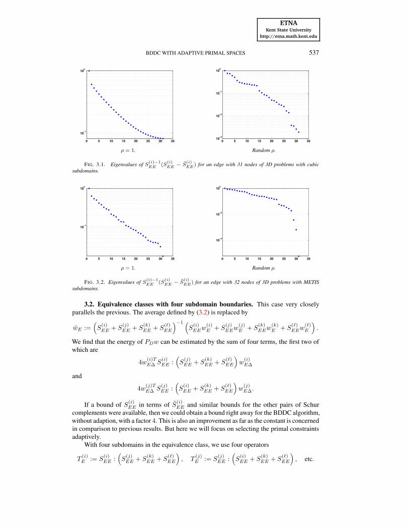
3.1. Some eigenvalue distributions. Following the example of Section 2.2, we havecomputed the eigenvalues of S(i)−1

EE (S(i)EE − S

(i)EE). The four plots provide information on the

eigenvalues of the generalized eigenvalue problem defined by S(i)EE and S(i)

EE in four differentcases.

We note that while in all cases we have one eigenvalue equal to 1, the decay of the restof the spectra is much less pronounced than for the faces. We note that a subdomain edgetypically will be associated with much fewer degrees of freedom than a subdomain face andthat therefore the need for a very rapid decay of these eigenvalues might be less important.




0 5 10 15 20 25 30 35

10−1

100

ρ = 1.

0 5 10 15 20 25 30 3510

−3

10−2

10−1

100

Random ρ.

FIG. 3.1. Eigenvalues of S(i)−1EE (S

(i)EE − S

(i)EE) for an edge with 31 nodes of 3D problems with cubic

subdomains.

0 5 10 15 20 25 30 35

10−1

100

ρ = 1.

0 5 10 15 20 25 30 35

10−4

10−2

100

Random ρ.

FIG. 3.2. Eigenvalues of S(i)−1EE (S

(i)EE − S

(i)EE) for an edge with 32 nodes of 3D problems with METIS

subdomains.

3.2. Equivalence classes with four subdomain boundaries. This case very closelyparallels the previous. The average defined by (3.2) is replaced by

wE :=(S

(i)EE + S

(j)EE + S

(k)EE + S

(`)EE

)−1 (S

(i)EEw

(i)E + S

(j)EEw

(j)E + S

(k)EEw

(k)E + S

(`)EEw

(`)E

).

We find that the energy of PDw can be estimated by the sum of four terms, the first two ofwhich are

4w(i)TE∆ S

(i)EE :

(S

(j)EE + S

(k)EE + S

(`)EE

)w

(i)E∆

and

4w(j)TE∆ S

(j)EE :

(S

(i)EE + S

(k)EE + S

(`)EE

)w

(j)E∆.

If a bound of S(i)EE in terms of S(i)

EE and similar bounds for the other pairs of Schurcomplements were available, then we could obtain a bound right away for the BDDC algorithm,without adaption, with a factor 4. This is also an improvement as far as the constant is concernedin comparison to previous results. But here we will focus on selecting the primal constraintsadaptively.

With four subdomains in the equivalence class, we use four operators

T(i)E := S

(i)EE :

(S

(j)EE + S

(k)EE + S

(`)EE

), T

(j)E := S

(j)EE :

(S

(i)EE + S

(k)EE + S

(`)EE

), etc.




All these operators are symmetric, positive definite, and they appear directly in our estimate ofthe energy of PDw. We can now use the trivial inequality

T(i)E ≤ T

(i)E + T

(j)E + T

(k)E + T

(`)E

and very similar bounds for the other terms and arrive at the generalized eigenvalue problem

(3.7)(S

(i)EE : S

(j)EE : S

(k)EE : S

(`)EE

)φ = λ

(T

(i)E + T

(j)E + T

(k)E + T

(`)E

)φ.

Both operators of (3.7) are symmetric with respect to the Schur complements. What willbe featured in the final bound would be the smallest eigenvalue not taken into account, i.e.,with eigenvectors not associated with the primal space, and a fixed factor similar to whatappears in the bounds of Lemmas 2.2 and 3.1 and Theorem 3.2.

LEMMA 3.3. Let λEtol be the smallest eigenvalue of (3.5) not chosen when selecting theprimal constraints for a subdomain edge E shared by four subdomains Ωi,Ωj , Ωk, and Ω`.We then have

‖(PDw)|E‖2S ≤4

λEtol(ai(w,w) + aj(w,w) + ak(w,w) + a`(w,w)) ,

where ai(·, ·) is the bilinear form associated to (1.1) and the subdomain Ωi, etc.We can now combine the estimates of Lemmas 2.2 and 3.3 into what is our main theoretical

result for this case.THEOREM 3.4. Assume that all subdomain edges are common to no more than four

subdomains. The S-norm of the operator PD then satisfies

‖PDw‖2S ≤( 2N2

F

minF λFtol+

8N2E

minE λEtol

)‖w‖2

S.

Here NF is the maximum number of faces of any subdomain, and NE is the maximum numberof edges. Therefore, the condition number of the deluxe BDDC algorithm satisfies

κ(M−1BDDC S

)≤ 2N2

F

minF λFtol+

8N2E

minE λEtol·

The proofs of this lemma and theorem follow exactly the same lines as those of Lemma 3.1and Theorem 3.2.

3.3. Recipes of some previous work. Several other generalized eigenvalue problemshave been employed quite successful but so far lack full theoretical justifications.

Scacchi and Zampini have used what would correspond to the operators S(i)EE : S

(j)EE : S

(k)EE

and S(i)EE + S

(j)EE + S

(k)EE or S(i)

EE : S(j)EE : S

(k)EE for difficult, very ill-conditioned problems

arising in isogeometric analysis. Stefano Zampini has also used S(i)EE : S

(j)EE : S

(k)EE and

S(i)EE : S

(j)EE : S

(k)EE successfully for subdomain edges and three-dimensional H(curl) prob-

lems; see [28]. So far, we have not found as full a justification for these recipes as for the onebased on using the generalized eigenvalue problems (2.2), (3.5), and (3.7).

4. Numerical results. We present some numerical results for our adaptive BDDC deluxealgorithm. We consider a triangulation of the unit cube into tetrahedral elements and decom-positions of this domain into cubic subdomains or subdomains obtained by using a METISmesh partitioner; see Figure 4.1.




METIS decomposition. One of the METIS subdomains.

FIG. 4.1. Domain decomposition obtained by METIS for the unit cube, N = 27.

Channels with ρ = 103. Coefficient distribution.

FIG. 4.2. Coefficient distribution with channels: black elements on the right have ρ = 103, and all the otherelements have ρ = 1.

We solve the resulting linear systems with random right-hand sides using BDDC pre-conditioners to a relative residual tolerance of 10−6. We always use a zero initial guess. Thenumber of iterations and condition number estimates (in parentheses) are reported for eachexperiment.

EXAMPLE 4.1. We first consider the scalability of the BDDC deluxe algorithm for a cubicsubdomain partitioning of the unit cube and for different standard choices of the primal space.The column label “Corners” represents the common choice with only primal constraints for thesubdomain vertices. “Edges” adds the average over each edge to the set of primal constraintswhile “Edges and Faces” additionally uses the averages over each face; see Table 4.1. We thencompare these results with adaptive algorithms based on generalized eigenvalue problems;see Table 4.2. The numbers in its first two columns represent the fraction of the range of theeigenvalues related to the subdomain edges that are incorporated into the primal space throughtheir eigenvectors. Thus, given the interval between the smallest and the largest eigenvalues,we use, as primal constraints, the eigenvectors of all the eigenvalues that lie in the leftmost 5%or 50% of this interval. For the faces, we always use a fixed 5%. Finally, for the last column,“Adaptive”, we use λFtol = (1 + log(H/h))−1, λEtol = (kH/h)−1, where k is the number ofsubdomains that share the edge E to select the eigenvalues. These formulas are borrowedfrom [12] and have allowed us to make direct comparisons with results of that study. We havealso found that this recipe selects a relatively small number of effective primal constraints.




TABLE 4.1Performance for different choices of primal constraints with H/h = 8 and cubic subdomains. NE is the

number of subdomain edges, and DOF is the number of degrees of freedom of the problem.

Corners Edges Edges and Faces NE DOFρ N I(κ) |WΠ| I(κ) |WΠ| I(κ) |WΠ|1 33 12(14.9) 8 12(13.9) 44 12(13.9) 98 36 15626

43 17(16.6) 27 17(15.6) 135 17(15.6) 279 108 3593753 24(17.2) 64 24(16.1) 304 23(16.1) 604 240 6892163 26(17.6) 125 25(16.5) 575 25(16.5) 1115 450 117649

R 33 23(42.9) 8 21(39.2) 44 23(39.1) 98 36 1562643 34(77.9) 27 33(64.8) 135 37(62.3) 279 108 3593753 51(83.4) 64 48(75.5) 304 51(75.2) 604 240 6892163 68(106) 125 66(90.0) 575 61(90.0) 1115 450 117649

S 33 24(176) 8 24(174) 44 23(173) 98 36 1562643 37(1068) 27 37(985) 135 33(981) 279 108 3593753 60(1994) 64 59(1812) 304 55(1804) 604 240 6892163 74(2234) 125 71(2022) 575 64(2013) 1115 450 117649

TABLE 4.2Scalability for adaptive primal constraints with H/h = 8 and cubic subdomains.

Primal 5% Primal 50% Adaptiveρ N I(κ) |WΠ| I(κ) |WΠ| I(κ) |WΠ| [f ]

1 33 6(1.5) 98 6(1.5) 122 8(2.2) 50 [0.6]43 6(1.5) 279 6(1.5) 333 8(2.2) 189[0.8]53 7(1.5) 604 6(1.5) 700 8(2.2) 460[0.9]63 7(1.5) 1115 7(1.5) 1265 8(2.1) 905[0.9]

R 33 14(5.9) 115 11(3.2) 213 10(2.5) 237[2.6]43 16(7.4) 336 13(7.3) 622 11(3.1) 746[3.0]53 19(12.1) 765 13(4.0) 1361 11(3.1) 1698[3.1]63 22(20.9) 1368 14(5.5) 2534 11(3.5) 3140[3.2]

S 33 9(10.5) 102 9(10.5) 119 10(10.6) 65[0.7]43 10(14.3) 285 10(13.8) 340 11(11.6) 197[0.8]53 11(15.2) 612 11(14.5) 708 11(15.2) 473[0.9]63 12(15.3) 1125 12(14.6) 1272 12(15.3) 918[0.9]

However, we note that in numerical experiments not reported here, we have found that thesmallest eigenvalues of the generalized eigenvalue problems for the subdomain edges remainabove a positive constant when H/h increases.

The number [f ] in square brackets represents the ratio of the dimension of the primalspace and the total number of edges and faces. Different choices of ρ are considered in allcases: ρ = 1, ρ = R (random values for each element), and ρ = S (a distribution with rodsand with jumps in the coefficients; see Figure 4.2). In the case of random values, we use auniform distribution to pick a number r in the interval [−3, 3] and then assign to each elementthe value 10r.

These experiments show that the standard choices of primal constraints can fail quitebadly for problems with a coefficient that varies considerably inside the subdomains. Theresults for the adaptive choices of primal constraints are much more satisfactory. We alsofind that we can have success with only a small number of primal constraints even for the




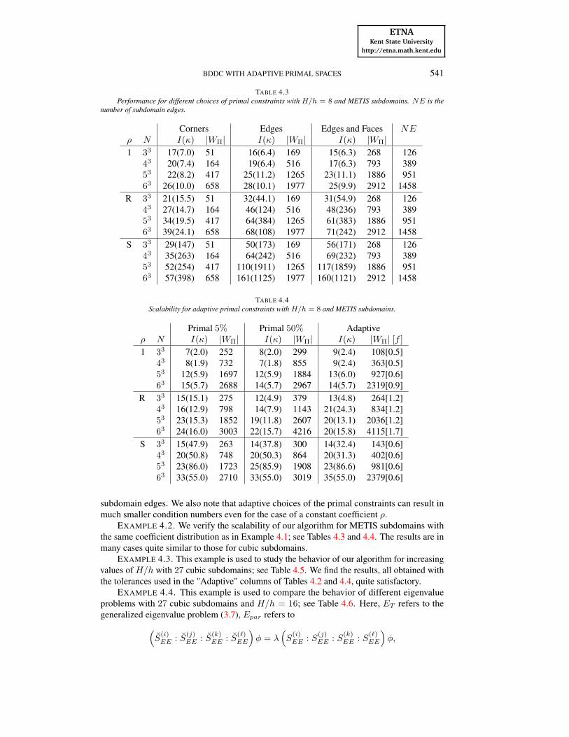
TABLE 4.3Performance for different choices of primal constraints with H/h = 8 and METIS subdomains. NE is the

number of subdomain edges.

Corners Edges Edges and Faces NEρ N I(κ) |WΠ| I(κ) |WΠ| I(κ) |WΠ|1 33 17(7.0) 51 16(6.4) 169 15(6.3) 268 126

43 20(7.4) 164 19(6.4) 516 17(6.3) 793 38953 22(8.2) 417 25(11.2) 1265 23(11.1) 1886 95163 26(10.0) 658 28(10.1) 1977 25(9.9) 2912 1458

R 33 21(15.5) 51 32(44.1) 169 31(54.9) 268 12643 27(14.7) 164 46(124) 516 48(236) 793 38953 34(19.5) 417 64(384) 1265 61(383) 1886 95163 39(24.1) 658 68(108) 1977 71(242) 2912 1458

S 33 29(147) 51 50(173) 169 56(171) 268 12643 35(263) 164 64(242) 516 69(232) 793 38953 52(254) 417 110(1911) 1265 117(1859) 1886 95163 57(398) 658 161(1125) 1977 160(1121) 2912 1458

TABLE 4.4Scalability for adaptive primal constraints with H/h = 8 and METIS subdomains.

Primal 5% Primal 50% Adaptiveρ N I(κ) |WΠ| I(κ) |WΠ| I(κ) |WΠ| [f ]

1 33 7(2.0) 252 8(2.0) 299 9(2.4) 108[0.5]43 8(1.9) 732 7(1.8) 855 9(2.4) 363[0.5]53 12(5.9) 1697 12(5.9) 1884 13(6.0) 927[0.6]63 15(5.7) 2688 14(5.7) 2967 14(5.7) 2319[0.9]

R 33 15(15.1) 275 12(4.9) 379 13(4.8) 264[1.2]43 16(12.9) 798 14(7.9) 1143 21(24.3) 834[1.2]53 23(15.3) 1852 19(11.8) 2607 20(13.1) 2036[1.2]63 24(16.0) 3003 22(15.7) 4216 20(15.8) 4115[1.7]

S 33 15(47.9) 263 14(37.8) 300 14(32.4) 143[0.6]43 20(50.8) 748 20(50.3) 864 20(31.3) 402[0.6]53 23(86.0) 1723 25(85.9) 1908 23(86.6) 981[0.6]63 33(55.0) 2710 33(55.0) 3019 35(55.0) 2379[0.6]

subdomain edges. We also note that adaptive choices of the primal constraints can result inmuch smaller condition numbers even for the case of a constant coefficient ρ.

EXAMPLE 4.2. We verify the scalability of our algorithm for METIS subdomains withthe same coefficient distribution as in Example 4.1; see Tables 4.3 and 4.4. The results are inmany cases quite similar to those for cubic subdomains.

EXAMPLE 4.3. This example is used to study the behavior of our algorithm for increasingvalues of H/h with 27 cubic subdomains; see Table 4.5. We find the results, all obtained withthe tolerances used in the "Adaptive" columns of Tables 4.2 and 4.4, quite satisfactory.

EXAMPLE 4.4. This example is used to compare the behavior of different eigenvalueproblems with 27 cubic subdomains and H/h = 16; see Table 4.6. Here, ET refers to thegeneralized eigenvalue problem (3.7), Epar refers to(

S(i)EE : S

(j)EE : S

(k)EE : S

(`)EE

)φ = λ

(S

(i)EE : S

(j)EE : S

(k)EE : S

(`)EE

)φ,




TABLE 4.5Results for the adaptive algorithm with 27 cubic subdomains for increasing values of H/h.

ρ = 1 ρ = R ρ = SH/h I(κ) |WΠ| [f ] I(κ) |WΠ| [f ] I(κ) |WΠ| [f ]

4 5(1.2) 62[0.7] 7(1.7) 154[1.7] 5(1.2) 62[0.7]8 8(2.2) 50[0.6] 10(2.5) 237[2.6] 10(10.7) 65[0.7]

12 9(2.7) 50[0.6] 12(4.0) 265[2.9] 11(19.7) 89[1.0]16 10(3.1) 50[0.6] 13(4.3) 270[3.0] 12(5.4) 60[0.7]

TABLE 4.6Results for different eigenvalue problems with N cubic subdomains and H/h = 8.

ET Epar Emixρ N I(κ) |WΠ| [f ] I(κ) |WΠ| [f ] I(κ) |WΠ| [f ]

1 33 8(2.1) 50[0.6] 8(2.1) 50[0.6] 8(2.2) 38[0.5]43 8(2.1) 189[0.8] 8(2.1) 189[0.8] 8(2.2) 141[0.6]53 8(2.1) 460[0.8] 8(2.1) 460[0.8] 8(2.2) 352[0.7]63 8(2.1) 905[0.9] 8(2.1) 905[0.9] 9(2.2) 713[0.7]

R 33 10(2.5) 237[2.6] 13(4.3) 71[0.8] 13(4.3) 59[0.7]43 11(7.3) 746[3.0] 15(9.6) 246[1.0] 14(4.4) 198[0.8]53 11(3.1) 1698[3.1] 16(8.8) 604[1.1] 14(4.8) 496[0.9]63 11(3.5) 3140[3.2] 18(10.3) 1158[1.2] 17(8.5) 966[1.0]

S 33 10(10.6) 65[0.7] 10(12.0) 57[0.7] 11(13.6) 41[0.5]43 11(11.6) 197[0.8] 14(30.0) 189[0.8] 14(29.1) 140[0.6]53 11(15.2) 473[0.9] 15(30.0) 463[0.9] 14(29.1) 354[0.7]63 12(15.3) 918[0.9] 17(30.0) 906[0.9] 16(29.4) 713[0.7]

and Emix to(S

(i)EE + S

(j)EE + S

(k)EE + S

(`)EE

)φ = λ

(S

(i)EE : S

(j)EE : S

(k)EE : S

(`)EE

)φ.

5. Conclusions. We have developed adaptive choices for the primal spaces for BDDCdeluxe methods and elliptic problems and a theoretical bound for the condition number of thepreconditioned system. We have first observed that adaptivity can considerably improve theperformance since classical choices with primal vertices, edge averages, and faces averagescan fail in case of large variations in the coefficients; see Table 4.1 and 4.3. Second, numericalexperiments show that the primal constraints related to the subdomain faces generally are easyto handle; this is supported by the discussion in Section 2.2. Therefore, the 5%-option hasbeen used in many of the experiments resulting in just one or two constraints per face in mostof the cases. For the subdomain edges, we note that there is no significant difference in thecase of constant coefficients if we use 5% or 50% of the interval. For the other two casesconsidered, extending this interval beyond 5% can be more important; it is clear that such anincrease will improve the condition number and the iteration count as illustrated in Tables 4.2and 4.4. Here, the results in the "Adaptive" column show that we can keep the primal spacesmall.

As we have already observed, the tolerances used for subdomain faces and edges seem towork well since they produce small primal spaces with good condition numbers. In most ofthe cases, the ratio between the dimension of the primal space and the total number of edgesand faces [f ] is smaller than 1, which means that, on average, we use fewer than one constraint




per subdomain face/edge. Finally, Table 4.6 exemplifies that different eigenvalue problemsconsidered by others can have a similar performance as ours.

Acknowledgments. The authors wishes to thank one of the referees who providedseveral suggestions that have helped improve our paper. They also wish to thank Dr. ClemensPechstein for the suggestion to use [24, Corollary 5.11] to improve our Lemma 2.2 and itsproof.

REFERENCES

[1] P. R. AMESTOY, I. S. DUFF, J.-Y. L’EXCELLENT, AND J. KOSTER, A fully asynchronous multifrontal solverusing distributed dynamic scheduling, SIAM J. Matrix Anal. Appl., 23 (2001), pp. 15–41.

[2] W. N. ANDERSON, JR. AND R. J. DUFFIN, Series and parallel addition of matrices, J. Math. Anal. Appl., 26(1969), pp. 576–594.

[3] W. N. ANDERSON, JR. AND G. E. TRAPP, Shorted operators. II, SIAM J. Appl. Math., 28 (1975), pp. 60–71.[4] L. BEIRÃO DA VEIGA, L. F. PAVARINO, S. SCACCHI, O. B. WIDLUND, AND S. ZAMPINI, Isogeometric

BDDC preconditioners with deluxe scaling, SIAM J. Sci. Comput., 36 (2014), pp. A1118–A1139.[5] , Adaptive selection of primal constraints for isogeometric BDDC deluxe preconditioners, SIAM J. Sci.

Comput., to appear, 2016.[6] S. C. BRENNER AND Q. HE, Lower bounds for three-dimensional nonoverlapping domain decomposition

algorithms, Numer. Math., 93 (2003), pp. 445–470.[7] C. R. DOHRMANN AND C. PECHSTEIN, Constraint and weight selection algorithms for BDDC, Talk by

C. R. Dohrmann in Rennes, France, June 2012.www.osti.gov/scitech/servlets/purl/1117109

[8] C. R. DOHRMANN AND O. B. WIDLUND, Some recent tools and a BDDC algorithm for 3D problems inH(curl), in Domain Decomposition Methods in Science and Engineering XX, R. E. Bank, M. Holst,O. Widlund, and J. Xu, eds., vol. 91 of Lect. Notes Comput. Sci. Eng., Springer, Heidelberg, 2013,pp. 15–26.

[9] A BDDC algorithm with deluxe scaling for three-dimensional H(curl) problems, Comm. Pure Appl.Math., 69 (2016), pp. 745–770.

[10] G. KARYPIS, R. AGGARWAL, K. SCHOEGEL, V. KUMAR, AND S. SHEKHAR, METIS home page.http://glaros.dtc.umn.edu/gkhome/views/metis

[11] H. H. KIM AND E. T. CHUNG, A BDDC algorithm with enriched coarse spaces for two-dimensional ellipticproblems with oscillatory and high contrast coefficients, Multiscale Model. Simul., 13 (2015), pp. 571–593.

[12] H. H. KIM, E. T. CHUNG, AND J. WANG, BDDC and FETI-DP algorithms with adaptive coarse spacesfor three-dimensional elliptic problems with oscillatory and high contrast coefficients, Preprint on arXiv,2015. http://arxiv.org/abs/1606.07560

[13] A. KLAWONN, M. KÜHN, AND O. RHEINBACH, Adaptive coarse spaces for FETI-DP in three dimensions,SIAM J. Sci. Comput., 38 (2016), pp. A2880–A2911.

[14] A. KLAWONN, P. RADTKE, AND O. RHEINBACH, A comparison of adaptive coarse spaces for iterativesubstructuring in two dimensions, Electron. Trans. Numer. Anal., 45 (2016), pp. 75–106.http://etna.ricam.oeaw.ac.at/vol.45.2016/pp75-106.dir/pp75-106.pdf

[15] A. KLAWONN, O. RHEINBACH, AND O. B. WIDLUND, An analysis of a FETI-DP algorithm on irregularsubdomains in the plane, SIAM J. Numer. Anal., 46 (2008), pp. 2484–2504.

[16] A. KLAWONN, O. B. WIDLUND, AND M. DRYJA, Dual-primal FETI methods for three-dimensional ellipticproblems with heterogeneous coefficients, SIAM J. Numer. Anal., 40 (2002), pp. 159–179.

[17] J. LI AND O. B. WIDLUND, FETI-DP, BDDC, and block Cholesky methods, Internat. J. Numer. MethodsEngrg., 66 (2006), pp. 250–271.

[18] J. MANDEL, C. R. DOHRMANN, AND R. TEZAUR, An algebraic theory for primal and dual substructuringmethods by constraints, Appl. Numer. Math., 54 (2005), pp. 167–193.

[19] J. MANDEL AND B. SOUSEDÍK, Adaptive selection of face coarse degrees of freedom in the BDDC andthe FETI-DP iterative substructuring methods, Comput. Methods Appl. Mech. Engrg., 196 (2007),pp. 1389–1399.

[20] J. MANDEL, B. SOUSEDÍK, AND J. ŠÍSTEK, Adaptive BDDC in three dimensions, Math. Comput. Simulation,82 (2012), pp. 1812–1831.

[21] J. NECAS, Les Méthodes Directes en Théorie des Équations Elliptiques, Academia, Prague, 1967.[22] D.-S. OH, O. B. WIDLUND, S. ZAMPINI, AND C. R. DOHRMANN, BDDC algorithms with deluxe scaling

and adaptive selection of primal constraints for Raviart-Thomas vector fields, Tech. Report TR2015-978,Courant Institute, New York University, 2015.

www.osti.gov/scitech/servlets/purl/1117109

http://glaros.dtc.umn.edu/gkhome/views/metis

http://arxiv.org/abs/1606.07560

http://etna.ricam.oeaw.ac.at/vol.45.2016/pp75-106.dir/pp75-106.pdf




[23] C. PECHSTEIN AND C. R. DOHRMANN, Modern domain decomposition methods, BDDC, deluxe scaling, andan algebraic approach, Talk by C. Pechstein at the University Linz, December 2013.http://people.ricam.oeaw.ac.at/c.pechstein/pechstein-bddc2013.pdf

[24] , A Unified Framework for Adaptive BDDC, Tech. Report 2016-20, Johann Radon Institute for Compu-tational and Applied Mathematics (RICAM), University Linz, 2016.https://www.ricam.oeaw.ac.at/files/reports/16/rep16-20.pdf

[25] Y. TIAN, How to express a parallel sum of k matrices, J. Math. Anal. Appl., 266 (2002), pp. 333–341.[26] A. TOSELLI AND O. WIDLUND, Domain Decomposition Methods—Algorithms and Theory, Springer, Berlin,

2005.[27] O. B. WIDLUND AND C. R. DOHRMANN, BDDC deluxe domain decomposition, in Domain Decomposition

Methods in Science and Engineering XXII, T. Dickopf, M. J. Gander, L. Halpern, R. Krause, L. F. Pavarino,eds., vol. 104 of Lecture Notes in Comput. Sci., Springer, Cham, 2016, pp. 93–103.

[28] S. ZAMPINI, Adaptive BDDC deluxe for H(curl), in Proceedings of the 23rd International Conference onDomain Decomposition Methods, 2015, to appear.

[29] , PCBDDC: a class of robust dual-primal preconditioners in PETSc, SIAM J. Sci. Comput., 38 (2016),pp. S282–S306.

http://people.ricam.oeaw.ac.at/c.pechstein/pechstein-bddc2013.pdf

https://www.ricam.oeaw.ac.at/files/reports/16/rep16-20.pdf

An adaptive choice of primal constraints for BDDC …etna.mcs.kent.edu/vol.45.2016/pp524-544.dir/pp524-544.pdfalso Section2.1. We note that algorithms using parallel sums for equivalence

Documents