An accurate and effective fmm-based approach for freehand 3d ultrasound reconstruction

Page 1

Au

TYa

b

c

ARRA

K3IF

1

bdtsawybi

mno

Sm

wy

1h

Biomedical Signal Processing and Control 8 (2013) 645– 656

Contents lists available at SciVerse ScienceDirect

Biomedical Signal Processing and Control

jou rn al h om epage: www.elsev ier .com/ locate /bspc

n accurate and effective FMM-based approach for freehand 3Dltrasound reconstruction�

iexiang Wena,b,c,1, Qingsong Zhua,c,1, Wenjian Qina,c, Ling Lia,c, Fan Yanga,b,c,aoqin Xiea,c, Jia Gua,c,∗

Shenzhen Institutes of Advanced Technology, Chinese Academy of Sciences, Shenzhen 518055, PR ChinaUniversity of Chinese Academy of Sciences, Beijing 100049, PR ChinaThe Shenzhen Key Laboratory for Low-cost Healthcare, Shenzhen 518055, PR China

a r t i c l e i n f o

rticle history:eceived 4 March 2013eceived in revised form 19 April 2013ccepted 24 May 2013

eywords:D ultrasound imagingnterpolation

a b s t r a c t

Freehand three-dimensional ultrasound imaging is a highly attractive research area because it is capableof volumetric visualization and analysis of tissues and organs. The reconstruction algorithm plays a keyrole to the construction of three-dimensional ultrasound volume data with higher image quality andfaster reconstruction speed. However, a systematic approach to such problem is still missing. A new fastmarching method (FMM) for three-dimensional ultrasound volume reconstruction using the tracked andhand-held probe is proposed in this paper. Our reconstruction approach consists of two stages: bin-fillingstage and hole-filling stage. Each pixel in the B-scan images is traversed and its intensity value is assigned

ast marching method to its nearest voxel in the bin-filling stage. For the efficient and accurate reconstruction, we present anew hole-filling algorithm based on the fast marching method. Our algorithm advances the interpolationboundary along its normal direction and fills the area closest to known voxel points in first, which ensurethat the structural details of image can be preserved. Experimental results on both ultrasonic abdominalphantom and in vivo urinary bladder of human subject and comparisons with some popular algorithmsare used to demonstrate its improvement in both reconstruction accuracy and efficiency.

. Introduction

Conventional two-dimensional (2D) ultrasound imaging haseen widely used for many clinical applications, such as medicaliagnosis, imaged-guided surgery. In comparison with computedomography (CT) and magnetic resonance imaging (MRI), ultra-ound imaging is non-invasive, non-ionizing, real-time, portable,nd low-cost. However, 2D ultrasound fails to offer physicians ahole volume data of tissues and organs for visualization and anal-

sis. Thus, three-dimensional (3D) ultrasound imaging system haseen developed to overcome such limitations by constructing var-

ous 3D datasets of anatomies for diagnosis in recent years [1–4].

� This is an open-access article distributed under the terms of the Creative Com-ons Attribution-NonCommercial-No Derivative Works License, which permits

on-commercial use, distribution, and reproduction in any medium, provided theriginal author and source are credited.∗ Corresponding author at: 1068 Xueyuan Avenue, Shenzhen University Town,

henzhen, PR China. Tel.: +86 755 86392278; fax: +86 755 86392299;obile: +86 15889622108.

E-mail addresses: [email protected] (T. Wen), [email protected] (Q. Zhu),[email protected] (W. Qin), [email protected] (L. Li), [email protected] (F. Yang),

[email protected] (Y. Xie), [email protected] (J. Gu).1 These authors contributed equally to this work.

746-8094/$ – see front matter © 2013 The Authors. Published by Elsevier Ltd. All rights ttp://dx.doi.org/10.1016/j.bspc.2013.05.009

© 2013 The Authors. Published by Elsevier Ltd. All rights reserved.

A number of approaches for constructing 3D ultrasound vol-ume data have been reported and empirically evaluated in [5].These approaches can be grouped into three categories: dedicated3D probes, mechanical scanning approach, and freehand scanningapproach. Although the systems using 3D probes usually equip anoscillating mechanism to sweep a predefined region of interested(ROI) and can provide 3D volume data in real-time, they are expen-sive and have limitation on scanning large volume organs [3]. Themechanical scanning based systems usually use the conventional2D transducer, which is translated or rotated by a stepping motorwhose position and orientation data are recorded synchronouslyin the scanning heads [6–8]. However, the mechanical scanningdevices are usually limited by their scanning range [3]. For free-hand 3D ultrasound, conventional 2D probe is integrated with apositioning sensor for labeling position and orientation of each B-scan image [1]. Freehand 3D ultrasound has received increasingattention for its low-cost, inherent flexibility nature in comparisonswith the dedicated 3D probes and mechanical scanning approaches.Freehand scanning allows the user to manipulate the transducerand view the desired anatomical section freely. During freehand

scanning, the 2D probe is manipulated by hand in an arbitrarilymanner. A sequence of B-scan images are then captured along withits corresponding position and orientation. The collection of irregu-larly sampled B-scan images is then used to reconstruct 3D regular

reserved.

Page 2

6 rocessing and Control 8 (2013) 645– 656

ga

3f2rniitptvmerirsbfiippeAtorfidoiDtatonwHisvaMsRdste

[idttwipmptt

46 T. Wen et al. / Biomedical Signal P

rids (i.e. volume data) by various interpolation or approximationlgorithms.

Volume reconstruction is the key procedure in the freehandD ultrasound systems. Various types of reconstruction algorithmsor compounding 3D ultrasound volume data from sequences ofD B-scans have been reported and evaluated in [9], where theseeconstruction algorithms are grouped into three categories: voxelearest neighbor (VNN) interpolation, pixel nearest neighbor (PNN)

nterpolation, and distance weighted (DW) interpolation. VNNnterpolation method is the most intuitive one and its implementa-ion is straightforward. It traverses on each voxel, finds its nearestixel by computing the shortest distance between the voxel andhe sampled B-scan image planes, and inserts the nearest pixelalue to the voxel [10]. Although VNN method can preserve theost original texture patterns from B-scan images (i.e. ultrasonic

cho corrupted with speckle noise), it also trends to generate largeeconstruction artifacts when the distance of the voxel to the B-scanmage plane is large. PNN interpolation method is the most populareconstruction algorithm, which traverses on each pixel in the B-can images and assigns the pixel value to its nearest voxel [11]. Theasic algorithm consists of two stages: bin-filling stage and hole-lling stage. In the bin-filling stage, each input pixel is traversed and

ts pixel value is assigned to its nearest voxel. For a voxel with multi-le pixel contribution, its value is usually the average of all assignedixel intensities. In the hole-filling stage, the algorithm traverses onach voxel and fills empty voxels by local neighborhood averaging.lthough the bin-filling technique can preserve the most original

exture pattern from the B-scan images, obvious artifacts can bebserved on the boundaries between the highly detailed bin-filledegion and the smoothed hole-filled region. Meanwhile, most hole-lling algorithms usually depend on the interpolation gaps. If theistance among sampled B-scan images is too far apart or the radiusf interpolation neighborhood is too small, there are still a few holesn the reconstructed volume data. Similar to the VNN interpolation,W interpolation proceeds voxel by voxel. But, instead of using

he nearest pixel, each voxel value is assigned with the weightedverage of a set of pixels from nearby B-scans [12]. The parame-ers to choose are the weighting function and the size and shapef the neighborhood. The simplest approach employs a sphericaleighborhood around each empty voxel. All pixels in the sphere areeighted by the inverse distance to the voxel and then averaged.owever, the determination of interpolation radius for the spher-

cal neighborhood is very empirical and subjective. If radius is toomall, it results in gaps. Yet if radius is too large, the reconstructedolume will be highly smoothed due to the effect of average oper-tion. These methods are designed to reduce computation time.ore elaborated methods are based on radial basis function, such as

pline interpolation function [13] or statistical Bayesian model withayleigh distribution [14]. Even though the elaborated method hasemonstrated its unique capability in image interpolation, speckleuppression, and edges preservation, it requires extremely compu-ation time due to the need to estimate the local parameters forach piecewise radial basis function.

This paper aims to develop a fast marching method (FMM)15] to the problem of freehand 3D ultrasound reconstruction. Wemplement our reconstruction framework with two-stage proce-ure to unify the VNN, PNN, and DW interpolation methods. Forhe bin-filling stage, voxels are filled with the data obtained fromhe irregularly sampled B-scan images. Most texture pattern can beell preserved in this stage as demonstrated in the VNN and PNN

nterpolation. For the hole-filling stage, we propose the FMM inter-olation algorithm [16,17] to interpolate empty voxels. During the

arching procedure, direction-weighted function is used to inter-

olate the nearby empty voxel. The marching direction ensureshat the interpolation propagates gray value in the normal direc-ion. Thus, the sharp edges in the image can be well preserved and

Fig. 1. The schematic diagram of the freehand 3D ultrasound imaging system.

the averaging tendency of the PNN and DW interpolation can beavoided. Although the FMM-based hole-filling technique has beenpublished before to the image inpainting domain, the applicationof such a method for 3D ultrasound reconstruction is new.

The rest of the paper is organized as follows. We detailthe freehand 3D ultrasound imaging system and the two-stagereconstruction procedure in Sections 2.1–2.3.1. The new FMMinterpolation method is presented in Section 2.3.2. The experi-mental studies and related evaluation results and discussions aredescribed in Section 3. The conclusions are made in Section 4.

2. System and methods

2.1. System setup

The freehand 3D ultrasound imaging system consists of threemodules: a conventional 2D ultrasound scanner (DC-7, MindrayMedical International Ltd., Shenzhen, China), an electromagneticspatial sensing device (Aurora, NDI, Ontario, Canada), and aworkstation with custom-designed software for data acquisition,volume reconstruction, and visualization. Fig. 1 illustrates the free-hand 3D ultrasound imaging system. The receiver of the spatialsensing device is attached to the 4.5 MHz hand-held probe of theultrasound scanner. The spatial information (i.e. position (x, y, z) andorientation (Rx, Ry, Rz)) between the receiver and transmitter arerecorded and transferred from the Aurora system control unit to theworkstation through its USB port. The real-time video stream of theultrasound scanner is digitalized by a video capture card (RGB-133,VTimage Inc., Shenzhen, China) installed in the workstation.

During data acquisition, spatial data and digitalized 2D B-scanimages are simultaneously recorded and collected in our custom-designed software programmed in C++ language. Since the devicesfor the collection of 2D B-scans and spatial data are indepen-dent, the temporal delay between the two data streams cannot beavoided. Meanwhile, the spatial relationship between the B-scanimage plane and magnetic position sensor needs to be determined.The temporal and spatial calibrations are performed using thecustom-designed phantoms for the feasibility and accuracy of thefreehand 3D ultrasound imaging system as described in [18,19].

2.2. Data acquisition

The output from the video capture card is a real-time videostream and each frame is a full screen view of the ultrasound scan-

ner. Due to the undesirable boundary (i.e. description informationlike patient’s name and exam date) in the full screen image, it isnecessary to crop the undesirable boundary using the rectanglecropping tools provided in our data acquisition software system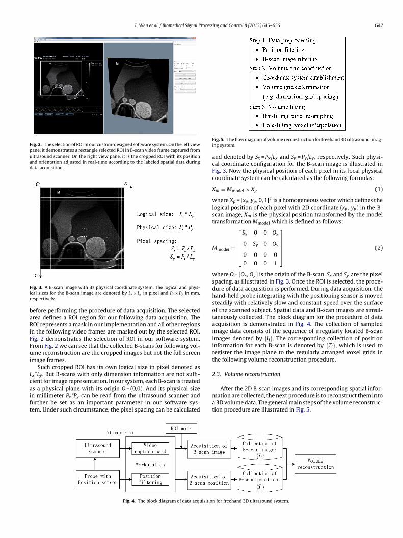

Page 3

T. Wen et al. / Biomedical Signal Processing and Control 8 (2013) 645– 656 647

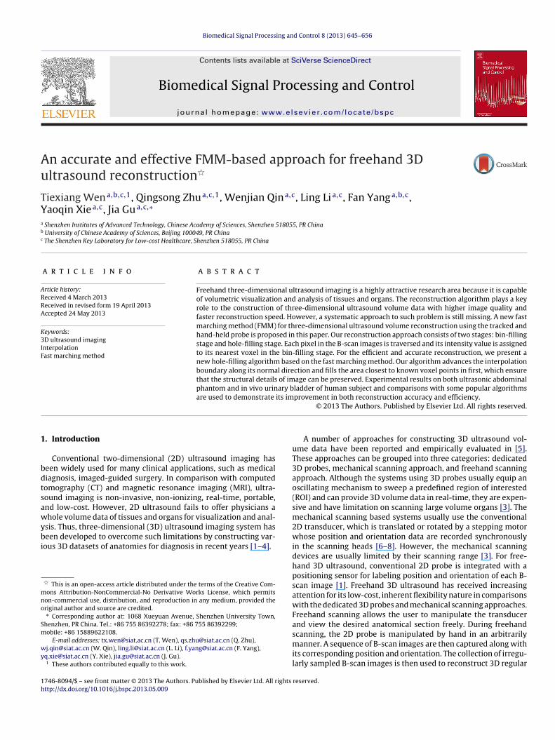
Fig. 2. The selection of ROI in our custom-designed software system. On the left viewpane, it demonstrates a rectangle selected ROI in B-scan video frame captured fromultrasound scanner. On the right view pane, it is the cropped ROI with its positionand orientation adjusted in real-time according to the labeled spatial data duringdata acquisition.

Fir

baRiFFui

Lcaift

ig. 3. A B-scan image with its physical coordinate system. The logical and phys-cal sizes for the B-scan image are denoted by Lx × Ly in pixel and Px × Py in mm,espectively.

efore performing the procedure of data acquisition. The selectedrea defines a ROI region for our following data acquisition. TheOI represents a mask in our implementation and all other regions

n the following video frames are masked out by the selected ROI.ig. 2 demonstrates the selection of ROI in our software system.rom Fig. 2 we can see that the collected B-scans for following vol-me reconstruction are the cropped images but not the full screen

mage frames.Such cropped ROI has its own logical size in pixel denoted as

x*Ly. But B-scans with only dimension information are not suffi-ient for image representation. In our system, each B-scan is treated

s a physical plane with its origin O = (0,0). And its physical sizen millimeter Px*Py can be read from the ultrasound scanner andurther be set as an important parameter in our software sys-em. Under such circumstance, the pixel spacing can be calculated

Fig. 4. The block diagram of data acquisitio

Fig. 5. The flow diagram of volume reconstruction for freehand 3D ultrasound imag-ing system.

and denoted by Sx = Px/Lx and Sy = Py/Ly, respectively. Such physi-cal coordinate configuration for the B-scan image is illustrated inFig. 3. Now the physical position of each pixel in its local physicalcoordinate system can be calculated as the following formulas:

Xm = Mmodel × Xp (1)

where Xp = [xp, yp, 0, 1]T is a homogeneous vector which defines thelogical position of each pixel with 2D coordinate (xp, yp) in the B-scan image, Xm is the physical position transformed by the modeltransformation Mmodel which is defined as follows:

Mmodel =

⎡⎢⎢⎢⎣

Sx 0 0 Ox

0 Sy 0 Oy

0 0 0 0

0 0 0 1

⎤⎥⎥⎥⎦ (2)

where O = [Ox, Oy] is the origin of the B-scan, Sx and Sy are the pixelspacing, as illustrated in Fig. 3. Once the ROI is selected, the proce-dure of data acquisition is performed. During data acquisition, thehand-held probe integrating with the positioning sensor is movedsteadily with relatively slow and constant speed over the surfaceof the scanned subject. Spatial data and B-scan images are simul-taneously collected. The block diagram for the procedure of dataacquisition is demonstrated in Fig. 4. The collection of sampledimage data consists of the sequence of irregularly located B-scanimages denoted by {Ii}. The corresponding collection of positioninformation for each B-scan is denoted by {Ti}, which is used toregister the image plane to the regularly arranged voxel grids inthe following volume reconstruction procedure.

2.3. Volume reconstruction

After the 2D B-scan images and its corresponding spatial infor-mation are collected, the next procedure is to reconstruct them intoa 3D volume data. The general main steps of the volume reconstruc-tion procedure are illustrated in Fig. 5.

n for freehand 3D ultrasound system.

Page 4

648 T. Wen et al. / Biomedical Signal Processing and Control 8 (2013) 645– 656

or bou

tStoTsistcfi

lvfptdwni(cimbcaipi

ii3sru

2

vita

u

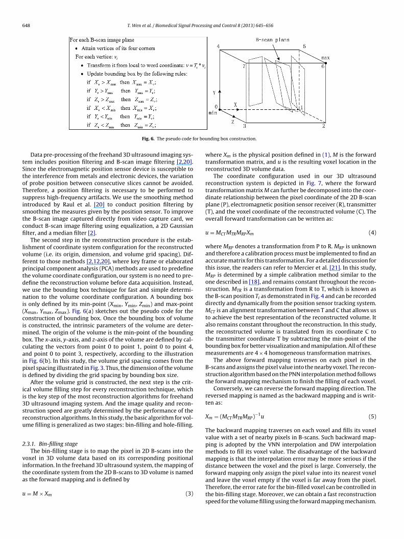
Fig. 6. The pseudo code f

Data pre-processing of the freehand 3D ultrasound imaging sys-em includes position filtering and B-scan image filtering [2,20].ince the electromagnetic position sensor device is susceptible tohe interference from metals and electronic devices, the variationf probe position between consecutive slices cannot be avoided.herefore, a position filtering is necessary to be performed touppress high-frequency artifacts. We use the smoothing methodntroduced by Raul et al. [20] to conduct position filtering bymoothing the measures given by the position sensor. To improvehe B-scan image captured directly from video capture card, weonduct B-scan image filtering using equalization, a 2D Gaussianlter, and a median filter [2].

The second step in the reconstruction procedure is the estab-ishment of coordinate system configuration for the reconstructedolume (i.e. its origin, dimension, and volume grid spacing). Dif-erent to those methods [2,12,20], where key frame or elaboratedrincipal component analysis (PCA) methods are used to predefinehe volume coordinate configuration, our system is no need to pre-efine the reconstruction volume before data acquisition. Instead,e use the bounding box technique for fast and simple determi-ation to the volume coordinate configuration. A bounding box

s only defined by its min-point (Xmin, Ymin, Zmin) and max-pointXmax, Ymax, Zmax). Fig. 6(a) sketches out the pseudo code for theonstruction of bounding box. Once the bounding box of volumes constructed, the intrinsic parameters of the volume are deter-

ined. The origin of the volume is the min-point of the boundingox. The x-axis, y-axis, and z-axis of the volume are defined by cal-ulating the vectors from point 0 to point 1, point 0 to point 4,nd point 0 to point 3, respectively, according to the illustrationn Fig. 6(b). In this study, the volume grid spacing comes from theixel spacing illustrated in Fig. 3. Thus, the dimension of the volume

s defined by dividing the grid spacing by bounding box size.After the volume grid is constructed, the next step is the crit-

cal volume filling step for every reconstruction technique, whichs the key step of the most reconstruction algorithms for freehandD ultrasound imaging system. And the image quality and recon-truction speed are greatly determined by the performance of theeconstruction algorithms. In this study, the basic algorithm for vol-me filling is generalized as two stages: bin-filling and hole-filling.

.3.1. Bin-filling stageThe bin-filling stage is to map the pixel in 2D B-scans into the

oxel in 3D volume data based on its corresponding positionalnformation. In the freehand 3D ultrasound system, the mapping ofhe coordinate system from the 2D B-scans to 3D volume is named

s the forward mapping and is defined by

= M × Xm (3)

nding box construction.

where Xm is the physical position defined in (1), M is the forwardtransformation matrix, and u is the resulting voxel location in thereconstructed 3D volume data.

The coordinate configuration used in our 3D ultrasoundreconstruction system is depicted in Fig. 7, where the forwardtransformation matrix M can further be decomposed into the coor-dinate relationship between the pixel coordinate of the 2D B-scanplane (P), electromagnetic position sensor receiver (R), transmitter(T), and the voxel coordinate of the reconstructed volume (C). Theoverall forward transformation can be written as:

u = MCT MTRMRPXm (4)

where MRP denotes a transformation from P to R. MRP is unknownand therefore a calibration process must be implemented to find anaccurate matrix for this transformation. For a detailed discussion forthis issue, the readers can refer to Mercier et al. [21]. In this study,MRP is determined by a simple calibration method similar to theone described in [18], and remains constant throughout the recon-struction. MTR is a transformation from R to T, which is known asthe B-scan position Ti as demonstrated in Fig. 4 and can be recordeddirectly and dynamically from the position sensor tracking system.MCT is an alignment transformation between T and C that allows usto achieve the best representation of the reconstructed volume. Italso remains constant throughout the reconstruction. In this study,the reconstructed volume is translated from its coordinate C tothe transmitter coordinate T by subtracting the min-point of thebounding box for better visualization and manipulation. All of thesemeasurements are 4 × 4 homogeneous transformation matrixes.

The above forward mapping traverses on each pixel in theB-scans and assigns the pixel value into the nearby voxel. The recon-struction algorithm based on the PNN interpolation method followsthe forward mapping mechanism to finish the filling of each voxel.

Conversely, we can reverse the forward mapping direction. Thereversed mapping is named as the backward mapping and is writ-ten as:

Xm = (MCT MTRMRP)−1u (5)

The backward mapping traverses on each voxel and fills its voxelvalue with a set of nearby pixels in B-scans. Such backward map-ping is adopted by the VNN interpolation and DW interpolationmethods to fill its voxel value. The disadvantage of the backwardmapping is that the interpolation error may be more serious if thedistance between the voxel and the pixel is large. Conversely, theforward mapping only assign the pixel value into its nearest voxel

and leave the voxel empty if the voxel is far away from the pixel.Therefore, the error rate for the bin-filled voxel can be controlled inthe bin-filling stage. Moreover, we can obtain a fast reconstructionspeed for the volume filling using the forward mapping mechanism.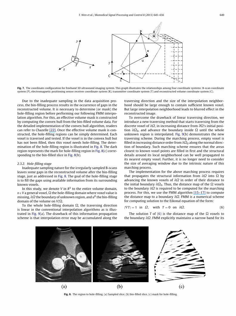

Page 5

T. Wen et al. / Biomedical Signal Processing and Control 8 (2013) 645– 656 649

F is gras smitte

crhlbtcsvhmrs

2

lsik

xmd

its

ig. 7. The coordinate configuration for freehand 3D ultrasound imaging system. Thystem (P), electromagnetic positioning sensor receiver coordinate system (R), tran

Due to the inadequate sampling in the data acquisition pro-ess, the bin-filling process results in the occurrence of gaps in theeconstructed volume. It is necessary to determine (or mask) theole-filling region before performing our following FMM interpo-

ation algorithm. For this, an effective volume mask is constructedy computing the convex hull from the bin-filled volume data. Forhe detailed implementation of the convex hull algorithm, readersan refer to Chazelle [22]. Once the effective volume mask is con-tructed, the hole-filling regions can be simply determined. Eachoxel is traversed and tested. If the voxel is in the convex hull butas not been filled, then this voxel needs hole-filling. The deter-ination of the hole-filling region is illustrated in Fig. 8. The dark

egion represents the mark for hole-filling region in Fig. 8(c) corre-ponding to the bin-filled slice in Fig. 8(b).

.3.2. Hole-filling stageInadequate sampling nature for the irregularly sampled B-scans

eaves some gaps in the reconstructed volume after the bin-fillingtage, just as addressed in Fig. 8. The goal of the hole-filling stages to fill the gaps using available information from its surroundingnown voxels.

In this study, we denote V in R3 to the entire volume domain, ∈ V a general voxel, � the hole-filling domain where voxel value isissing, ∂ ̋ the boundary of unknown region, and u0 the bin-filling

omain of the volume on V/�.

To the whole hole-filling domain �, the traversing direction

s linear in the conventional interpolation algorithms as is illus-rated in Fig. 9(a). The drawback of this information propagationcheme is that interpolation error may be accumulated along the

Fig. 8. The region to hole-filling. (a) Sampled slice

ph illustrates the relationships among four coordinate systems: B-scan coordinater coordinate system (T) and reconstructed volume coordinate system (C).

traversing direction and the size of the interpolation neighbor-hood should be large enough to contain sufficient known voxel.But large interpolation neighborhood leads to blurred effect in thereconstructed image.

To overcome the drawback of linear traversing direction, weintroduce a new traversing method that starts traversing from thediscrete voxel of ∂˝, in increasing distance from ∂�’s initial posi-tion ∂˝0, and advance the boundary inside � until the wholeunknown region is interpolated. Fig. 9(b) demonstrates the newtraversing scheme. During the marching process, empty voxel isfilled in increasing distance order from ∂˝0 along the normal direc-tion of boundary. Such marching scheme ensures that the areasclosest to known voxel points are filled in first and the structuraldetails around its local neighborhood can be well propagated toits nearest empty voxel. Further, it is no longer need to considerthe size of averaging window due to the intrinsic nature of thismarching process.

The implementation for the above marching process requiresthat propagates the structural information from ∂ ̋ into � byadvancing the known voxels of ∂ ̋ in order of their distance tothe initial boundary ∂˝0. Thus, the distance map of the � voxelsto the boundary ∂ ̋ is required to be computed for the marchingprocess. For this, we use the FMM algorithm [15–17] to computethe distance map to a boundary ∂˝. FMM is a numerical schemefor computing solution to the Eikonal equation of the form:

|∇T | = 1 in ˝, with T = 0 on ∂˝. (6)

The solution T of (6) is the distance map of the � voxels tothe boundary ∂˝. FMM explicitly maintains a narrow band for its

, (b) bin-filled slice, (c) mask for hole-filling.

Page 6

650 T. Wen et al. / Biomedical Signal Processing and Control 8 (2013) 645– 656

Fig. 9. Advancing direction of information. (a) Information propagation direction for conventional interpolation algorithm in the hole-filling stage. u0 is the given domainw boundd interp

sn

t

m

jTntatug

bpvi

G

hich has been filled in the bin-filling stage, ̋ is the unknown region and ∂ ̋ is theirection for the proposed fast marching scheme, where the marching direction of

urface evolution. Moreover, the gradient of T (i.e. �T) is exactly theormal to ∂˝.

Following the idea of upwind approximation for the gradient,he finite difference equation of (6) is written as:

ax (D−xT, D+xT, 0)2 + max (D−yT, D+yT, 0)2

+ max (D−zT, D+zT, 0)2 = 1 (7)

where D−xT(i, j, k) = T(i, j, k) − T(i − 1, j, k) and D−xT(i, j, k) = T(i + 1,, k) − T(i, j, k) are the backward and forward operators in x direction.he operators D−yT, D+yT, D−zT, and D+zT in the y and x coordi-ate directions are similar to those defined in the x direction. Usinghe upwind scheme, each new T value u in the evolving bound-ry ∂ ̋ is updated by solving (7) for its eight octants and retainshe smallest solution. Fig. 10 gives the illustrative formulas of thepdating computation in each octant configuration with its volumerid representation.

The aim of hole-filling stage is to estimate the empty voxel valueased on its neighborhood voxels. We consider now how to inter-olate a newly discovered empty voxel as a function of the knownoxels around it during the fast marching process. The general

nterpolation formulas can be written as:

(p) =∑n

i=1ωiG(qi)∑ni=1ωi

(8)

Fig. 10. The illustration of the discret

ary (or surface) between known and unknown region. (b) Information propagationolation is along with the normal direction of the boundary.

where G(p) is the gray value of the empty voxel p situated onthe evolving boundary ∂ ̋ of the hole-filling region, n the numberof voxels situated within the predefine spherical region centeredabout voxel p, G(qi) the gray value of the known voxel at the i-th volume coordinate qi, and ωi the weight for the i-th voxel. Thedesign of the weight ωi is crucial to propagate the sharp details forthe hole-filling process. For example, we can employ the local aver-aged weighting function, the inverse distance weighting function,and the squared distance weighting function.

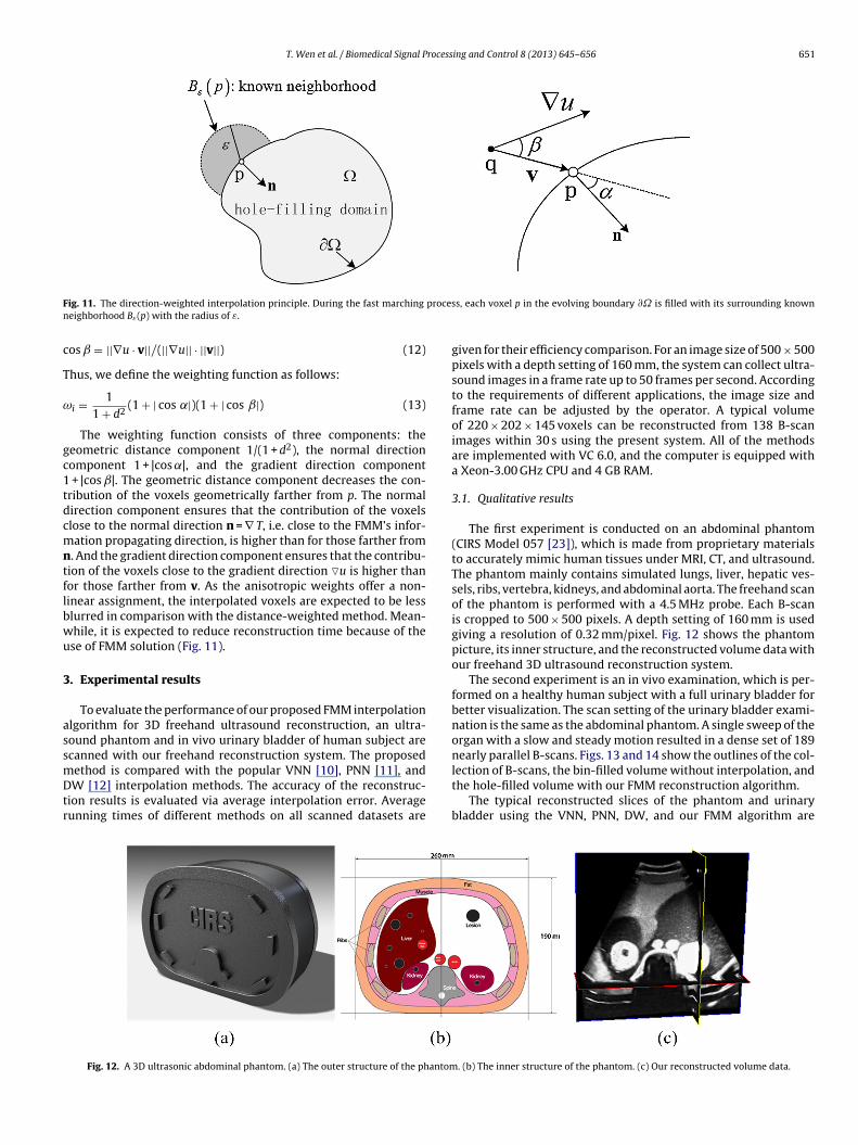
To preserve the sharp structure details better, a new direction-weighted function is introduced. Fig. 10 illustrates the direction-weighted interpolation principle. The gray estimation on p shouldbe determined by the values of the known voxels close to p, i.e. inBε(p), which denotes a spherical region with radius ε around p. Fora known voxel q in the spherical region, i.e. q ∈ Bε(p), we use thefollowing Euclidian distance between p(xp, yp, zp) and q(xq, yq, zq):

d =√

(xp − xq)2 + (yp − yq)2 + (zp − zq)2 (9)

And the vector v from q to p is written as:

v = (vx, vy, vz) = (xp − xq, yp − yq, zp − zq) (10)

Denote n the normal to ∂ ̋ and �u the gradient value of the givenpoint q. Then the angles are defined from these vectors as:

cos ̨ = ||n · v||/(||n|| · ||v||) (11)

e solution of Eikonal equation.

Page 7

T. Wen et al. / Biomedical Signal Processing and Control 8 (2013) 645– 656 651

F procesn

c

T

ω

gc1tdcmntflbwu

3

assmDtr

ig. 11. The direction-weighted interpolation principle. During the fast marching

eighborhood Bε(p) with the radius of ε.

os ̌ = ||∇u · v||/(||∇u|| · ||v||) (12)

hus, we define the weighting function as follows:

i = 11 + d2

(1 + | cos ˛|)(1 + | cos ˇ|) (13)

The weighting function consists of three components: theeometric distance component 1/(1 + d2), the normal directionomponent 1 + |cos ˛|, and the gradient direction component

+ |cos ˇ|. The geometric distance component decreases the con-ribution of the voxels geometrically farther from p. The normalirection component ensures that the contribution of the voxelslose to the normal direction n = ∇ T, i.e. close to the FMM’s infor-ation propagating direction, is higher than for those farther from

. And the gradient direction component ensures that the contribu-ion of the voxels close to the gradient direction �u is higher thanor those farther from v. As the anisotropic weights offer a non-inear assignment, the interpolated voxels are expected to be lesslurred in comparison with the distance-weighted method. Mean-hile, it is expected to reduce reconstruction time because of these of FMM solution (Fig. 11).

. Experimental results

To evaluate the performance of our proposed FMM interpolationlgorithm for 3D freehand ultrasound reconstruction, an ultra-ound phantom and in vivo urinary bladder of human subject arecanned with our freehand reconstruction system. The proposed

ethod is compared with the popular VNN [10], PNN [11], andW [12] interpolation methods. The accuracy of the reconstruc-

ion results is evaluated via average interpolation error. Averageunning times of different methods on all scanned datasets are

Fig. 12. A 3D ultrasonic abdominal phantom. (a) The outer structure of the phantom

s, each voxel p in the evolving boundary ∂ ̋ is filled with its surrounding known

given for their efficiency comparison. For an image size of 500 × 500pixels with a depth setting of 160 mm, the system can collect ultra-sound images in a frame rate up to 50 frames per second. Accordingto the requirements of different applications, the image size andframe rate can be adjusted by the operator. A typical volumeof 220 × 202 × 145 voxels can be reconstructed from 138 B-scanimages within 30 s using the present system. All of the methodsare implemented with VC 6.0, and the computer is equipped witha Xeon-3.00 GHz CPU and 4 GB RAM.

3.1. Qualitative results

The first experiment is conducted on an abdominal phantom(CIRS Model 057 [23]), which is made from proprietary materialsto accurately mimic human tissues under MRI, CT, and ultrasound.The phantom mainly contains simulated lungs, liver, hepatic ves-sels, ribs, vertebra, kidneys, and abdominal aorta. The freehand scanof the phantom is performed with a 4.5 MHz probe. Each B-scanis cropped to 500 × 500 pixels. A depth setting of 160 mm is usedgiving a resolution of 0.32 mm/pixel. Fig. 12 shows the phantompicture, its inner structure, and the reconstructed volume data withour freehand 3D ultrasound reconstruction system.

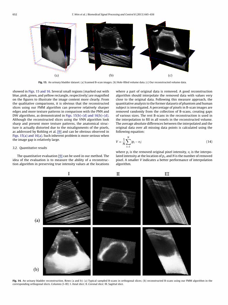
The second experiment is an in vivo examination, which is per-formed on a healthy human subject with a full urinary bladder forbetter visualization. The scan setting of the urinary bladder exami-nation is the same as the abdominal phantom. A single sweep of theorgan with a slow and steady motion resulted in a dense set of 189nearly parallel B-scans. Figs. 13 and 14 show the outlines of the col-

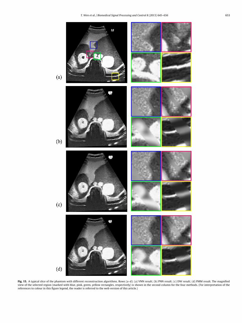
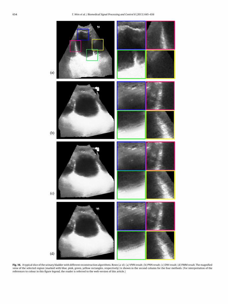
lection of B-scans, the bin-filled volume without interpolation, andthe hole-filled volume with our FMM reconstruction algorithm.

The typical reconstructed slices of the phantom and urinarybladder using the VNN, PNN, DW, and our FMM algorithm are

. (b) The inner structure of the phantom. (c) Our reconstructed volume data.

Page 8

652 T. Wen et al. / Biomedical Signal Processing and Control 8 (2013) 645– 656

es. (b)

sbotseDAstaFt

3

it

Fc

Fig. 13. An urinary bladder dataset. (a) Scanned B-scan imag

howed in Figs. 15 and 16. Several small regions (marked out withlue, pink, green, and yellow rectangle, respectively) are magnifiedn the figures to illustrate the image content more clearly. Fromhe qualitative comparisons, it is obvious that the reconstructedlices using our FMM algorithm can preserve relatively sharperdges and more texture patterns in comparison with the PNN andW algorithms, as demonstrated in Figs. 15(b)–(d) and 16(b)–(d).lthough the reconstructed slices using the VNN algorithm lookharp and present more texture patterns, the anatomical struc-ure is actually distorted due to the misalignments of the pixels,s addressed by Rohling et al. [9] and can be obvious observed inigs. 15(a) and 16(a). Such inherent problem is more serious whenhe image gap is relatively large.

.2. Quantitative results

The quantitative evaluation [9] can be used in our method. Thedea of the evaluation is to measure the ability of a reconstruc-ion algorithm in preserving true intensity values at the locations

ig. 14. An urinary bladder reconstruction. Rows (a and b): (a) Typical sampled B-scanorresponding orthogonal slices. Columns (I–III): I. Axial slice; II. Coronal slice; III. Sagitta

Hole-filled volume data. (c) Our reconstructed volume data.

where a part of original data is removed. A good reconstructionalgorithm should interpolate the removed data with values veryclose to the original data. Following this measure approach, thequantitative analysis to the former datasets of phantom and humansubject is investigated. A percentage of pixels in B-scan images areremoved randomly from the collection of B-scans, creating gapsof various sizes. The rest B-scans in the reconstruction is used inthe interpolation to fill in all voxels in the reconstructed volume.The average absolute differences between the interpolated and theoriginal data over all missing data points is calculated using thefollowing equation:

V = 1N

N∑i=1

|pi − vi| (14)

where pi is the removed original pixel intensity, vi is the interpo-lated intensity at the location of pi, and N is the number of removedpixel. A smaller V indicates a better performance of interpolationalgorithm.

s in orthogonal slices; (b) reconstructed B-scans using our FMM algorithm in thel slice.

Page 9

T. Wen et al. / Biomedical Signal Processing and Control 8 (2013) 645– 656 653

Fig. 15. A typical slice of the phantom with different reconstruction algorithms. Rows (a–d): (a) VNN result; (b) PNN result; (c) DW result; (d) FMM result. The magnifiedview of the selected region (marked with blue, pink, green, yellow rectangles, respectively) is shown in the second column for the four methods. (For interpretation of thereferences to colour in this figure legend, the reader is referred to the web version of this article.)

Page 10

654 T. Wen et al. / Biomedical Signal Processing and Control 8 (2013) 645– 656

Fig. 16. A typical slice of the urinary bladder with different reconstruction algorithms. Rows (a–d): (a) VNN result; (b) PNN result; (c) DW result; (d) FMM result. The magnifiedview of the selected region (marked with blue, pink, green, yellow rectangles, respectively) is shown in the second column for the four methods. (For interpretation of thereferences to colour in this figure legend, the reader is referred to the web version of this article.)

Page 11

T. Wen et al. / Biomedical Signal Processing and Control 8 (2013) 645– 656 655

Table 1The averaged interpolation error V for the abdominal phantom using the VNN, PNN,DW, and FMM algorithms. � is the mean of V and � is the standard deviation.

VNN PNN DW FMM

� � � � � � � �

0% 0.00 0.00 0.00 0.00 0.00 0.00 0.00 0.0025% 5.62 0.72 5.55 0.82 5.23 0.78 3.37 0.7450% 7.15 0.79 5.99 0.85 5.77 0.82 3.77 0.8175% 7.78 0.94 6.18 0.91 6.14 0.89 4.12 0.87100% 8.47 0.98 7.01 1.11 6.92 1.09 4.87 1.13

aFBtatwtbec

aPtrfcmTu1m

3

saeacaocpPi

TT

Table 3Computational time complexity for VNN, DW, PNN, and FMM algorithms. Nx , Ny , Nz

are the dimensions of the volume grid in x, y, and z direction, Np is the number ofthe acquired 2D B-scan images, R is the size of the spherical interpolation region.

Time complexity Method

VNN PNN DW FMM

O(N · Np) O(N · R) O(N · Np · R) O(M · log(M) · R)

Note. N = Nx · Ny · Nz , M = max(Nx , Ny , Nz).

Table 4Average computation times (in seconds) for the phantom using the VNN, PNN,DW, and FMM algorithms. DW2 represents the two-stage methodology for distant-weighted interpolation algorithm.

VNN PNN DW DW2 FMM

� � � � � � � � � �

300% 9.94 0.97 8.52 0.96 8.81 0.94 6.85 0.91500% 10.83 1.17 9.66 1.12 9.25 1.03 7.71 1.12700% 11.28 1.12 10.96 1.20 10.62 1.11 8.42 1.13

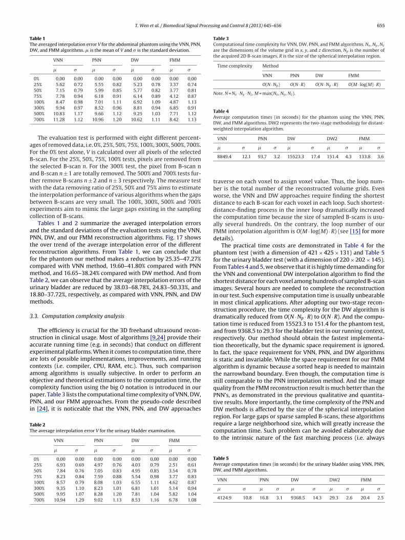
The evaluation test is performed with eight different percent-ges of removed data, i.e. 0%, 25%, 50%, 75%, 100%, 300%, 500%, 700%.or the 0% test alone, V is calculated over all pixels of the selected-scan. For the 25%, 50%, 75%, 100% tests, pixels are removed fromhe selected B-scan n. For the 300% test, the pixel from B-scan nnd B-scan n ± 1 are totally removed. The 500% and 700% tests fur-her remove B-scans n ± 2 and n ± 3 respectively. The measure testith the data removing ratio of 25%, 50% and 75% aims to estimate

he interpolation performance of various algorithms when the gapsetween B-scans are very small. The 100%, 300%, 500% and 700%xperiments aim to mimic the large gaps existing in the samplingollection of B-scans.

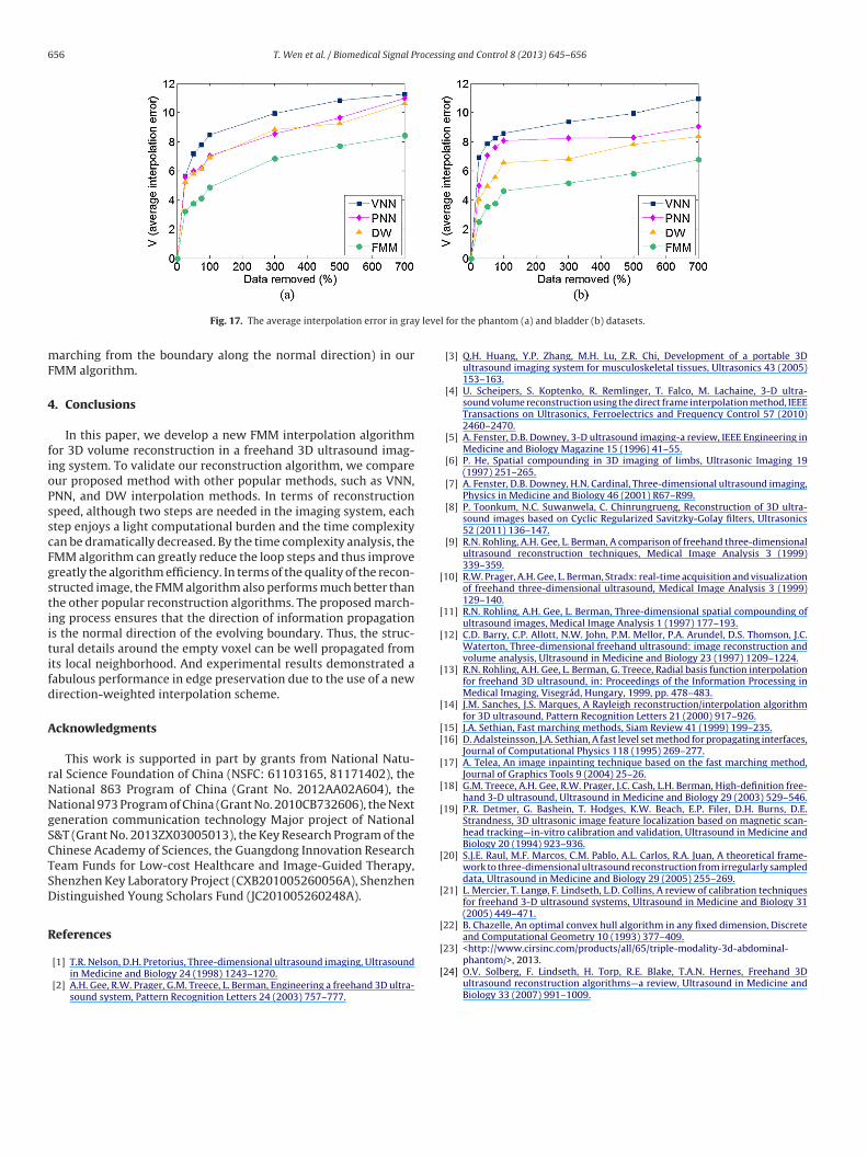
Tables 1 and 2 summarize the averaged interpolation errorsnd the standard deviations of the evaluation tests using the VNN,NN, DW, and our FMM reconstruction algorithms. Fig. 17 showshe over trend of the average interpolation error of the differenteconstruction algorithms. From Table 1, we can conclude thator the phantom our method makes a reduction by 25.35–47.27%ompared with VNN method, 19.60–41.80% compared with PNNethod, and 16.65–38.24% compared with DW method. And from

able 2, we can observe that the average interpolation errors of therinary bladder are reduced by 38.03–68.78%, 24.83–50.33%, and8.80–37.72%, respectively, as compared with VNN, PNN, and DWethods.

.3. Computation complexity analysis

The efficiency is crucial for the 3D freehand ultrasound recon-truction in clinical usage. Most of algorithms [9,24] provide theirccurate running time (e.g. in seconds) that conduct on differentxperimental platforms. When it comes to computation time, therere lots of possible implementations, improvements, and runningontexts (i.e. compiler, CPU, RAM, etc.). Thus, such comparisonmong algorithms is usually subjective. In order to perform anbjective and theoretical estimations to the computation time, the

omplexity function using the big O notation is introduced in ouraper. Table 3 lists the computational time complexity of VNN, DW,NN, and our FMM approaches. From the pseudo-code describedn [24], it is noticeable that the VNN, PNN, and DW approaches

able 2he average interpolation error V for the urinary bladder examination.

VNN PNN DW FMM

� � � � � � � �

0% 0.00 0.00 0.00 0.00 0.00 0.00 0.00 0.0025% 6.93 0.69 4.97 0.76 4.03 0.79 2.51 0.6150% 7.84 0.76 7.05 0.83 4.95 0.85 3.54 0.7875% 8.23 0.84 7.59 0.88 5.54 0.98 3.77 0.83100% 8.57 0.79 8.08 1.03 6.55 1.11 4.62 0.87300% 9.35 1.10 8.23 1.01 6.81 1.01 5.14 0.94500% 9.95 1.07 8.28 1.20 7.81 1.04 5.82 1.04700% 10.94 1.29 9.02 1.13 8.53 1.16 6.78 1.08

8849.4 12.1 93.7 3.2 15523.3 17.4 151.4 4.3 133.8 3.6

traverse on each voxel to assign voxel value. Thus, the loop num-ber is the total number of the reconstructed volume grids. Evenworse, the VNN and DW approaches require finding the shortestdistance to each B-scan for each voxel in each loop. Such shortest-distance-finding process in the inner loop dramatically increasedthe computation time because the size of sampled B-scans is usu-ally several hundreds. On the contrary, the loop number of ourFMM interpolation algorithm is O(M · log(M) · R) (see [15] for moredetails).

The practical time costs are demonstrated in Table 4 for thephantom test (with a dimension of 421 × 425 × 131) and Table 5for the urinary bladder test (with a dimension of 220 × 202 × 145).From Tables 4 and 5, we observe that it is highly time demanding forthe VNN and conventional DW interpolation algorithm to find theshortest distance for each voxel among hundreds of sampled B-scanimages. Several hours are needed to complete the reconstructionin our test. Such expensive computation time is usually unbearablein most clinical applications. After adopting our two-stage recon-struction procedure, the time complexity for the DW algorithm isdramatically reduced from O(N · Np · R) to O(N · R). And the compu-tation time is reduced from 15523.3 to 151.4 for the phantom test,and from 9368.5 to 29.3 for the bladder test in our running context,respectively. Our method should obtain the fastest implementa-tion theoretically, but the dynamic space requirement is ignored.In fact, the space requirement for VNN, PNN, and DW algorithmsis static and invariable. While the space requirement for our FMMalgorithm is dynamic because a sorted heap is needed to maintainthe narrowband boundary. Even though, the computation time isstill comparable to the PNN interpolation method. And the imagequality from the FMM reconstruction result is much better than thePNN’s, as demonstrated in the previous qualitative and quantita-tive results. More importantly, the time complexity of the PNN andDW methods is affected by the size of the spherical interpolationregion. For large gaps or sparse sampled B-scans, these algorithmsrequire a large neighborhood size, which will greatly increase the

computation time. Such problem can be avoided elaborately dueto the intrinsic nature of the fast marching process (i.e. always

Table 5Average computation times (in seconds) for the urinary bladder using VNN, PNN,DW, and FMM algorithms.

VNN PNN DW DW2 FMM

� � � � � � � � � �

4124.9 10.8 16.8 3.1 9368.5 14.3 29.3 2.6 20.4 2.5

Page 12

656 T. Wen et al. / Biomedical Signal Processing and Control 8 (2013) 645– 656

y leve

mF

4

fioPsscFgstiitifd

A

rNNgSCTSD

R

[

[

[

[

[

[[

[

[

[

[

[

[

Fig. 17. The average interpolation error in gra

arching from the boundary along the normal direction) in ourMM algorithm.

. Conclusions

In this paper, we develop a new FMM interpolation algorithmor 3D volume reconstruction in a freehand 3D ultrasound imag-ng system. To validate our reconstruction algorithm, we compareur proposed method with other popular methods, such as VNN,NN, and DW interpolation methods. In terms of reconstructionpeed, although two steps are needed in the imaging system, eachtep enjoys a light computational burden and the time complexityan be dramatically decreased. By the time complexity analysis, theMM algorithm can greatly reduce the loop steps and thus improvereatly the algorithm efficiency. In terms of the quality of the recon-tructed image, the FMM algorithm also performs much better thanhe other popular reconstruction algorithms. The proposed march-ng process ensures that the direction of information propagations the normal direction of the evolving boundary. Thus, the struc-ural details around the empty voxel can be well propagated fromts local neighborhood. And experimental results demonstrated aabulous performance in edge preservation due to the use of a newirection-weighted interpolation scheme.

cknowledgments

This work is supported in part by grants from National Natu-al Science Foundation of China (NSFC: 61103165, 81171402), theational 863 Program of China (Grant No. 2012AA02A604), theational 973 Program of China (Grant No. 2010CB732606), the Nexteneration communication technology Major project of National&T (Grant No. 2013ZX03005013), the Key Research Program of thehinese Academy of Sciences, the Guangdong Innovation Researcheam Funds for Low-cost Healthcare and Image-Guided Therapy,henzhen Key Laboratory Project (CXB201005260056A), Shenzhenistinguished Young Scholars Fund (JC201005260248A).

eferences

[1] T.R. Nelson, D.H. Pretorius, Three-dimensional ultrasound imaging, Ultrasoundin Medicine and Biology 24 (1998) 1243–1270.

[2] A.H. Gee, R.W. Prager, G.M. Treece, L. Berman, Engineering a freehand 3D ultra-sound system, Pattern Recognition Letters 24 (2003) 757–777.

[

[

l for the phantom (a) and bladder (b) datasets.

[3] Q.H. Huang, Y.P. Zhang, M.H. Lu, Z.R. Chi, Development of a portable 3Dultrasound imaging system for musculoskeletal tissues, Ultrasonics 43 (2005)153–163.

[4] U. Scheipers, S. Koptenko, R. Remlinger, T. Falco, M. Lachaine, 3-D ultra-sound volume reconstruction using the direct frame interpolation method, IEEETransactions on Ultrasonics, Ferroelectrics and Frequency Control 57 (2010)2460–2470.

[5] A. Fenster, D.B. Downey, 3-D ultrasound imaging-a review, IEEE Engineering inMedicine and Biology Magazine 15 (1996) 41–55.

[6] P. He, Spatial compounding in 3D imaging of limbs, Ultrasonic Imaging 19(1997) 251–265.

[7] A. Fenster, D.B. Downey, H.N. Cardinal, Three-dimensional ultrasound imaging,Physics in Medicine and Biology 46 (2001) R67–R99.

[8] P. Toonkum, N.C. Suwanwela, C. Chinrungrueng, Reconstruction of 3D ultra-sound images based on Cyclic Regularized Savitzky-Golay filters, Ultrasonics52 (2011) 136–147.

[9] R.N. Rohling, A.H. Gee, L. Berman, A comparison of freehand three-dimensionalultrasound reconstruction techniques, Medical Image Analysis 3 (1999)339–359.

10] R.W. Prager, A.H. Gee, L. Berman, Stradx: real-time acquisition and visualizationof freehand three-dimensional ultrasound, Medical Image Analysis 3 (1999)129–140.

11] R.N. Rohling, A.H. Gee, L. Berman, Three-dimensional spatial compounding ofultrasound images, Medical Image Analysis 1 (1997) 177–193.

12] C.D. Barry, C.P. Allott, N.W. John, P.M. Mellor, P.A. Arundel, D.S. Thomson, J.C.Waterton, Three-dimensional freehand ultrasound: image reconstruction andvolume analysis, Ultrasound in Medicine and Biology 23 (1997) 1209–1224.

13] R.N. Rohling, A.H. Gee, L. Berman, G. Treece, Radial basis function interpolationfor freehand 3D ultrasound, in: Proceedings of the Information Processing inMedical Imaging, Visegrád, Hungary, 1999, pp. 478–483.

14] J.M. Sanches, J.S. Marques, A Rayleigh reconstruction/interpolation algorithmfor 3D ultrasound, Pattern Recognition Letters 21 (2000) 917–926.

15] J.A. Sethian, Fast marching methods, Siam Review 41 (1999) 199–235.16] D. Adalsteinsson, J.A. Sethian, A fast level set method for propagating interfaces,

Journal of Computational Physics 118 (1995) 269–277.17] A. Telea, An image inpainting technique based on the fast marching method,

Journal of Graphics Tools 9 (2004) 25–26.18] G.M. Treece, A.H. Gee, R.W. Prager, J.C. Cash, L.H. Berman, High-definition free-

hand 3-D ultrasound, Ultrasound in Medicine and Biology 29 (2003) 529–546.19] P.R. Detmer, G. Bashein, T. Hodges, K.W. Beach, E.P. Filer, D.H. Burns, D.E.

Strandness, 3D ultrasonic image feature localization based on magnetic scan-head tracking—in-vitro calibration and validation, Ultrasound in Medicine andBiology 20 (1994) 923–936.

20] S.J.E. Raul, M.F. Marcos, C.M. Pablo, A.L. Carlos, R.A. Juan, A theoretical frame-work to three-dimensional ultrasound reconstruction from irregularly sampleddata, Ultrasound in Medicine and Biology 29 (2005) 255–269.

21] L. Mercier, T. Langø, F. Lindseth, L.D. Collins, A review of calibration techniquesfor freehand 3-D ultrasound systems, Ultrasound in Medicine and Biology 31(2005) 449–471.

22] B. Chazelle, An optimal convex hull algorithm in any fixed dimension, Discreteand Computational Geometry 10 (1993) 377–409.

23] <http://www.cirsinc.com/products/all/65/triple-modality-3d-abdominal-phantom/>, 2013.

24] O.V. Solberg, F. Lindseth, H. Torp, R.E. Blake, T.A.N. Hernes, Freehand 3Dultrasound reconstruction algorithms—a review, Ultrasound in Medicine andBiology 33 (2007) 991–1009.