An abundance exchange model of fish assemblage response to changing habitat along embayment–stream gradients of Lake Ontario, New York

Page 1

Arg

ND

a

A

R

R

6

A

P

K

M

D

A

H

F

E

L

1

Tooi1aC

0d

e c o l o g i c a l m o d e l l i n g 2 0 1 ( 2 0 0 7 ) 453–467

avai lab le at www.sc iencedi rec t .com

journa l homepage: www.e lsev ier .com/ locate /eco lmodel

n abundance exchange model of fish assemblageesponse to changing habitat along embayment–streamradients of Lake Ontario, New York

uanchan Singkran ∗

epartment of Natural Resources, Cornell University, 105 Rice Hall, Ithaca, NY 14853, USA

r t i c l e i n f o

rticle history:

eceived 10 June 2006

eceived in revised form

October 2006

ccepted 17 October 2006

ublished on line 22 November 2006

eywords:

odel

istribution

bundance exchange

abitat preference

ish assemblages

mbayment–stream

a b s t r a c t

A spatially explicit abundance exchange model (AEM) was developed to predict distribution

patterns of five fish species in relation to their population characteristics and habitat prefer-

ences along two embayment–stream gradients associated with Lake Ontario, New York. The

five fish species were yellow perch (Perca flavescens), bluegill (Lepomis macrochirus), logperch

(Percina caprodes), bluntnose minnow (Pimephales notatus), and fantail darter (Etheostoma fla-

bellare). Preference indexes of each target fish species for water depth, water temperature,

current velocity, cover types (aquatic plants, algae, and woody debris), and bottom substrates

(mud, sand, gravel-cobble, and rock-bedrock) were estimated from the field observations,

and these were used to compute habitat preference (HP) of the associated fish species. Fish

HP was a key variable in the AEM to quantify abundance exchange of an associated fish

species among habitats on each study gradient. According to the results, the AEM efficiently

determined local distribution ranges of the fish species on one study gradient. Results from

the model validation showed that the AEM with its estimated parameters was able to quan-

tify most of the fish species distributions on the second gradient. Overall, the AEM is rigorous

ake Ontario for quantifying the distribution patterns of the target species along the changing habitat

gradients. With its flexible structure that is applicable for array functions and differential

equations from both static and dynamic components, the AEM can be modified to deter-

mine patterns of organism distribution in complex systems with different environments

and geography.

and Gurney, 1982; Tilman and Kareiva, 1997), few empiri-

. Introduction

he influence of changing landscapes and environmentsn organism distribution across ecotones (transition zones)f contrasting habitats (e.g., grassland–forest) has been

ncreasingly studied in terrestrial ecosystems (e.g., Clements,

905; Leopold, 1933; Odum, 1971; Risser, 1990; Johnson etl., 1992; Lidicker, 1999; Fortin et al., 2000; Harding, 2002;adenasso et al., 2003; Ries et al., 2004), whereas fewer stud-

∗ Tel.: +1 607 255 2042; fax: +1 415 532 1435.E-mail address: [email protected].

304-3800/$ – see front matter © 2006 Elsevier B.V. All rights reserved.oi:10.1016/j.ecolmodel.2006.10.012

© 2006 Elsevier B.V. All rights reserved.

ies of this similar research type have been conducted inaquatic ecosystems (Winemiller and Leslie, 1992; Willis andMagnuson, 2002; Martino and Able, 2003; Miller and Sadro,2003). Additionally, although distribution of organisms is akey mechanism underlying the population dynamics (Nisbet

cal studies (Reyes et al., 1994; Gaff et al., 2000; Kupschus,2003) have quantitatively determined organism distributionin association with both changes in habitat and population

Page 2

i n g

ST gradient includes Sterling Pond and Sterling Creek. The

454 e c o l o g i c a l m o d e l l

characteristics (birth, death, and migration) over space andtime.

In this study, an abundance exchange model (AEM) wasbuilt to quantify the distribution of fish species assemblagesin relation to both population characteristics and habitatpreferences of fish across lentic–lotic transitions on twoembayment–stream gradients associated with Lake Ontario,New York. For purposes of this study, the term “transition”referred to both abrupt and gradual changes in spatial habitatheterogeneity between lentic (embayment) and lotic (stream)systems on the study gradients. As a result, this transition isoften distinctly observed at the lentic–lotic periphery, and itmay gradually or abruptly occur across the zone of transitionbetween the two systems.

The objectives of developing the spatially explicit AEMwere to determine how changing habitat influences dis-tribution patterns of fish species assemblages along theembayment–stream gradients and how population character-istics shape the size of fish population over time. To test ifthe AEM could efficiently capture distribution patterns of fishacross different habitat conditions, five fish species, yellowperch (Perca flavescens), bluegill (Lepomis macrochirus), logperch(Percina caprodes), bluntnose minnow (Pimephales notatus), andfantail darter (Etheostoma flabellare) were selected for model-ing. Yellow perch and bluegill commonly distributed in theembayment-downstream parts on both study gradients. Log-perch was mainly observed at the downstream-middle part onone study gradient, but this species was not observed on thesecond gradient. Bluntnose minnow commonly distributedthroughout both study gradients, while fantail darter mainlydistributed at the upstream parts of both study gradients.

In aquatic systems, high variability in hydrology (Wiens,2002) and climate-linked seasonal changes can alter otheraquatic habitat variables (e.g., water temperature and growthof aquatic plants and algae). As a result, the migration rateof fish along a gradient is most likely to reflect fish habi-tat preference within a dynamic template. Additionally, ithas been considered that each fish species has a specificrange of distribution (e.g., Morrison et al., 1985; Guay etal., 2000); the species stays within its range but will vari-ably distribute among habitats therein. This conforms tononlinear patterns of organism distribution along changinghabitat gradients (Whittaker, 1975; Lewis, 1997). In this study,both dynamic habitat variables (water depth, water tem-perature, current velocity, aquatic plants, algae, and woodydebris) and static habitat variables (the bottom substrates, i.e.,mud, sand, gravel-cobble, and rock-bedrock) were observedalong the study gradients and used to estimate fish habitatpreferences.

To test the hypothesis that distributions of fish acrosslentic–lotic transitions on the study gradients are based on fishpreferences for changing habitats within their local ranges,habitat preferences of the target fish species at two life stages(0+ years and 1+ years) were the key variable in the AEM toquantify distribution patterns of the associated fish speciesalong each study gradient. STELLA® 7.0.3 Research (High

Performance Systems Inc., 2002) was used to run the AEM.Since it was developed by Barry Richmond in 1985, STELLAhas been widely used by scientists across fields of study.This software is capable of simulating many components and

2 0 1 ( 2 0 0 7 ) 453–467

interactions of complex systems, and is fast and efficient atcalculating a diversity of array functions and differential equa-tions (e.g., Reyes et al., 1994; Pan and Raynal, 1995; Marın,1997; Gottlieb, 1998; Ford, 1999; Krivtsov et al., 2000; Dew, 2001;Gertseva et al., 2003, 2004; Kilpatrick et al., 2004; McCauslandet al., 2006).

Besides model development and prediction, model valida-tion, an important modeling process (Haefner, 1996; Oldenet al., 2002; Ottaviani et al., 2004), was the other objectiveof this study. Although numerous modeling approaches (e.g.,statistics, system dynamics, geographic information system(GIS)) have been used for modeling species distribution, fewof the models were further validated after the predictionswere completed (Olden et al., 2002). Model validation is cru-cial for evaluating the accuracy of the model’s predictions andfuture applicability (Olden et al., 2002; Ottaviani et al., 2004). Inaddition, proper ways of validating the model must be imple-mented. To verify that the model prediction is robust andunbiased and has minimal errors (i.e., over-fitting data, over-rating model performance, or underestimating the error forfuture application), one must validate the model with an inde-pendent data set that has not been previously used to estimatethe model’s parameters (Guisan and Zimmermann, 2000; Elithand Burgman, 2002; Fielding, 2002; Olden et al., 2002; Ottavianiet al., 2004).

In this study, to evaluate if the AEM is robust and effi-cient for predicting the distribution of the target fish speciesin similar geographic and hydrologic systems, the model withits estimated parameters to quantify the distribution patternof each target species on one study gradient was validatedagainst the observed data of the same fish species on the sec-ond study gradient located in close proximity. Accuracy ofthe model prediction was determined using the chi-square(�2) statistic to test the goodness of fit between predictedand observed percentage abundances of fish along each studygradient. The important modeling processes and the modelperformance presented in this study may contribute to appli-cations for better predicting the distribution of fish speciesassemblages across different habitats. This knowledge willhelp resource managers evaluate and maximize healthy habi-tats among different aquatic ecosystems to support diversefish assemblages at both local and regional scales.

2. Study gradients and field observations

The empirical studies were conducted across lentic–lotic tran-sitions on two embayment–stream gradients: Floodwood (FL)and Sterling (ST) gradients, located on the southeastern coastof Lake Ontario, New York (Fig. 1). The FL gradient comprisesFloodwood Pond and Sandy Creek. The total watershed areafor the FL gradient was 671.82 km2, and the surface area ofFloodwood Pond alone was 0.078 km2. Sandy Creek rangesin width from 6 m (upstream) to more than 50 m (enteringFloodwood Pond) and has a mean annual discharge of 7.8 m3/s(37-year record—USGS gage 04250750 above study area). The

total watershed area associated with the ST gradient was210.76 km2, and the surface area of Sterling Pond alone was0.38 km2. Sterling Creek ranges in width from 3 m (upstream)

Page 3

e c o l o g i c a l m o d e l l i n g 2 0 1 ( 2 0 0 7 ) 453–467 455

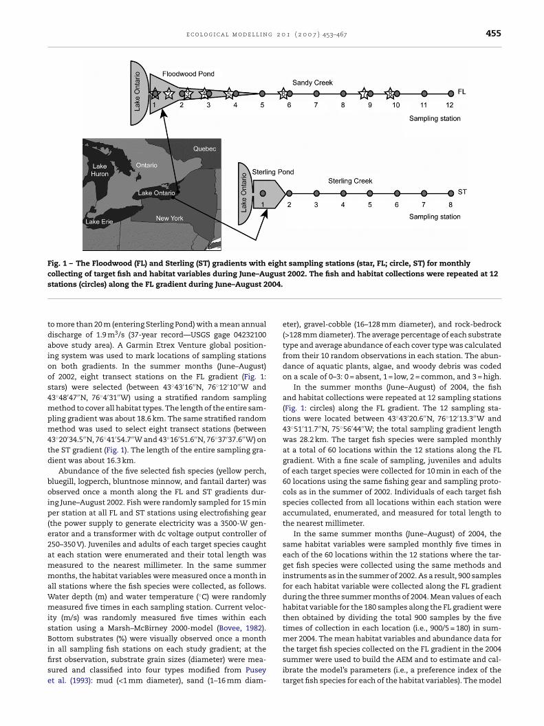
Fig. 1 – The Floodwood (FL) and Sterling (ST) gradients with eight sampling stations (star, FL; circle, ST) for monthlycollecting of target fish and habitat variables during June–August 2002. The fish and habitat collections were repeated at 12s 004.

tdaioos4mpm4td

boip(e2ammaWmisBifise

tations (circles) along the FL gradient during June–August 2

o more than 20 m (entering Sterling Pond) with a mean annualischarge of 1.9 m3/s (37-year record—USGS gage 04232100bove study area). A Garmin Etrex Venture global position-ng system was used to mark locations of sampling stationsn both gradients. In the summer months (June–August)f 2002, eight transect stations on the FL gradient (Fig. 1:tars) were selected (between 43◦43′16′′N, 76◦12′10′′W and3◦48′47′′N, 76◦4′31′′W) using a stratified random samplingethod to cover all habitat types. The length of the entire sam-

ling gradient was about 18.6 km. The same stratified randomethod was used to select eight transect stations (between

3◦20′34.5′′N, 76◦41′54.7′′W and 43◦16′51.6′′N, 76◦37′37.6′′W) onhe ST gradient (Fig. 1). The length of the entire sampling gra-ient was about 16.3 km.

Abundance of the five selected fish species (yellow perch,luegill, logperch, bluntnose minnow, and fantail darter) wasbserved once a month along the FL and ST gradients dur-

ng June–August 2002. Fish were randomly sampled for 15 miner station at all FL and ST stations using electrofishing gear

the power supply to generate electricity was a 3500-W gen-rator and a transformer with dc voltage output controller of50–350 V). Juveniles and adults of each target species caughtt each station were enumerated and their total length waseasured to the nearest millimeter. In the same summeronths, the habitat variables were measured once a month in

ll stations where the fish species were collected, as follows.ater depth (m) and water temperature (◦C) were randomlyeasured five times in each sampling station. Current veloc-

ty (m/s) was randomly measured five times within eachtation using a Marsh–McBirney 2000-model (Bovee, 1982).ottom substrates (%) were visually observed once a month

n all sampling fish stations on each study gradient; at therst observation, substrate grain sizes (diameter) were mea-ured and classified into four types modified from Puseyt al. (1993): mud (<1 mm diameter), sand (1–16 mm diam-

eter), gravel-cobble (16–128 mm diameter), and rock-bedrock(>128 mm diameter). The average percentage of each substratetype and average abundance of each cover type was calculatedfrom their 10 random observations in each station. The abun-dance of aquatic plants, algae, and woody debris was codedon a scale of 0–3: 0 = absent, 1 = low, 2 = common, and 3 = high.

In the summer months (June–August) of 2004, the fishand habitat collections were repeated at 12 sampling stations(Fig. 1: circles) along the FL gradient. The 12 sampling sta-tions were located between 43◦43′20.6′′N, 76◦12′13.3′′W and43◦51′11.7′′N, 75◦56′44′′W; the total sampling gradient lengthwas 28.2 km. The target fish species were sampled monthlyat a total of 60 locations within the 12 stations along the FLgradient. With a fine scale of sampling, juveniles and adultsof each target species were collected for 10 min in each of the60 locations using the same fishing gear and sampling proto-cols as in the summer of 2002. Individuals of each target fishspecies collected from all locations within each station wereaccumulated, enumerated, and measured for total length tothe nearest millimeter.

In the same summer months (June–August) of 2004, thesame habitat variables were sampled monthly five times ineach of the 60 locations within the 12 stations where the tar-get fish species were collected using the same methods andinstruments as in the summer of 2002. As a result, 900 samplesfor each habitat variable were collected along the FL gradientduring the three summer months of 2004. Mean values of eachhabitat variable for the 180 samples along the FL gradient werethen obtained by dividing the total 900 samples by the fivetimes of collection in each location (i.e., 900/5 = 180) in sum-mer 2004. The mean habitat variables and abundance data for

the target fish species collected on the FL gradient in the 2004summer were used to build the AEM and to estimate and cal-ibrate the model’s parameters (i.e., a preference index of thetarget fish species for each of the habitat variables). The model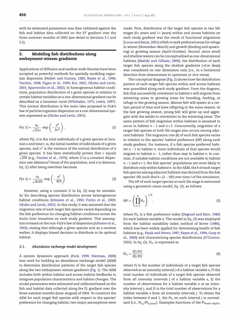

Page 4

i n g

456 e c o l o g i c a l m o d e l l

with its estimated parameters was then validated against thefish and habitat data collected on the ST gradient over thethree summer months of 2002 (see detail in Sections 3.1 and3.2).

3. Modeling fish distributions alongembayment–stream gradients

Applications of diffusion and random walk theories have beenaccepted as powerful methods for spatially modeling organ-ism dispersion (Nisbet and Gurney, 1982; Reyes et al., 1994;Turchin, 1998; Fagan et al., 1999; Kot, 2001; Okubo and Levin,2001; Sparrevohn et al., 2002). In homogeneous habitat condi-tions, population distribution of a given species in relation tocertain habitat variables on a one-dimensional gradient can bedescribed as a Gaussian curve (Whittaker, 1975; Lewis, 1997).This normal distribution is the main idea proposed in Fick’slaw of particle/organism dispersion on a one-dimensional sys-tem expressed as (Okubo and Levin, 2001):

P(x, t) = n0√2��

exp

(− x2

2�2

), (1)

where P(x, t) is the total individuals of a given species at loca-tion x and time t, n0 the initial number of individuals of a givenspecies, and �2 is the variance of the normal distribution of agiven species. It has been statistically proven that � equals√

2Dt (e.g., Fischer et al., 1979), where D is a constant disper-sion rate (distance2/time) of the population, and x is distance.Eq. (1) after being rewritten becomes

P(x, t) = n0√4�Dt

exp

(− x2

4Dt

)(2)

However, using a constant D in Eq. (2) may be unrealis-tic for describing species distribution across heterogeneoushabitat conditions (Johnson et al., 1992; Fortin et al., 2000;Okubo and Levin, 2001). In this study, it was assumed that themigration rate of each target fish species varied depending onthe fish preference for changing habitat conditions across thelentic–lotic transition on each study gradient. This assump-tion is based on the non-Fick’s law of dispersion (Johnson et al.,1992), stating that although a given species acts as a randomwalker, it displays biased decision to distribute to its optimalhabitat.

3.1. Abundance exchange model development

A system dynamics approach (Ford, 1999; Sterman, 2000)was used for building an abundance exchange model (AEM)to determine distribution patterns of the target fish speciesalong the two embayment–stream gradients (Fig. 1). The AEMincludes both within-habitat and across-habitat feedbacks tointegrate population characteristics and habitat changes. Themodel parameters were estimated and calibrated based on the

fish and habitat data collected along the FL gradient over thethree summer months (June–August) of 2004. To construct theAEM for each target fish species with respect to the species’preference for changing habitat, two major assumptions were

2 0 1 ( 2 0 0 7 ) 453–467

made. First, distribution of the target fish species at two lifestages (0+ years and 1+ years) within and across habitats oneach study gradient was the result of functional migrations(Lucas and Baras, 2001) of fish to seek preferred areas for refugein winter (November–March) and growth (feeding and spawn-ing) in growing season (April–October). Second, since smalland shallow waters can be conceptualized as one-dimensionalhabitats (Skalski and Gilliam, 2000), the distribution of eachtarget fish species along the shallow gradients (<6 m deep)was considered on one dimension only (i.e., in a horizontaldirection from downstream to upstream or vice versa).

The conceptual diagram (Fig. 2) shows how the distributionpattern of each target fish species within and across habitatswas quantified along each study gradient. From the diagram,fish that successfully overwinter in habitat n will migrate fromwintering areas to growing areas for breeding, feeding, orrefuge in the growing season. Mature fish will spawn at a cer-tain period of time and have offspring in the same season. Inthe late growing season, young fish will grow up and aggre-gate with the adults to overwinter in the wintering areas. Thesame pattern of fish migration within habitats is assumed tooccur in habitat n − 1 and n + 1. Concurrently, migration of atarget fish species at both life stages also occurs among adja-cent habitats. The migration rate (k) of each fish species variesin relation to the species’ habitat preference (HP) along eachstudy gradient. For instance, if a fish species preferred habi-tat n − 1 to habitat n, more individuals of that species wouldmigrate to habitat n − 1, rather than stay in habitat n. In con-trast, if suitable habitat conditions are not available in habitatn − 1 and n + 1, the fish species’ populations are most likely todistribute only within habitat n. In the AEM, the k of each targetfish species among adjacent habitats was derived from the fishspecies’ HP, such that k = (1 − HP) over time t of the simulation.

The HP of each target species at each life stage is estimatedusing a geometric mean model, Eq. (3), as follows:

HP =(

N∏x=1

Pix

)1/N

, (3)

where Pix is a fish preference index (Degraaf and Bain, 1986)for each habitat variable x. The model in Eq. (3) was employedfrom the habitat suitability index method of Bovee (1986),which has been widely applied for determining health of fishhabitats (e.g., Pajak and Neves, 1987; Reyes et al., 1994; Guay etal., 2000) and characterizing species distributions (O’Connor,2002). In Eq. (3), Pix, is expressed as

Pix = (Fj/Ft)(Ej/Et)

, (4)

where Fj is the number of individuals of a target fish speciesobserved at an intensity interval j of a habitat variable x, Ft thetotal number of individuals of a target fish species observedfrom all intensity intervals j of a habitat variable x, Ej thenumber of observations for a habitat variable x at an inten-

sity interval j, and Et is the total number of observations for ahabitat variable x from all intensity intervals j. To obtain theindex between 0 and 1, the Pix on each interval j is normal-ized (i.e., Pix,j/Pix,jmax). Examples functions of the Piwater depth,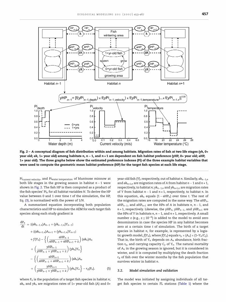

Page 5

e c o l o g i c a l m o d e l l i n g 2 0 1 ( 2 0 0 7 ) 453–467 457

Fig. 2 – A conceptual diagram of fish distribution within and among habitats. Migration rates of fish at two life stages (yk, 0+year old; ak, 1+ year old) among habitats n, n − 1, and n + 1 are dependent on fish habitat preference (yHP, 0+ year old; aHP,1 ferew e (H

PbstvE

cs

wa

+ year old). The three graphs below show the estimated preere used to compute the geometric mean habitat preferenc

icurrent velocity, and Piwater temperature of bluntnose minnow atoth life stages in the growing season in habitat n − 1 werehown in Fig. 2. The fish HP is then computed as a product ofhe fish species’ Pix for all habitat variables N. To derive the HPalue between 0 and 1 over time t of the simulation, the HP,q. (3), is normalized with the power of 1/N.

A summarized equation incorporating both populationharacteristics and HP to simulate the AEM for each target fishpecies along each study gradient is

dPn

dt= {(akn−1,n)An−1 + (ykn−1,n)Yn−1}

+ {(akn+1,n)An+1 + (ykn+1,n)Yn+1}

+ f (Yn) −{(

aHPn−1

aHPn−1 + aHPn+1 + z

)(akn)An

+(

yHPn−1

yHPn−1 + yHPn+1 + z

)(ykn)Yn

}−{(

aHPn+1

aHPn−1 + aHPn+1 + z

)(akn)An( ) }

+ yHPn+1

yHPn−1 + yHPn+1 + z(ykn)Yn − rd(Pn), (5)

here Pn is the population of a target fish species in habitat n;kn and ykn are migration rates of 1+ year-old fish (A) and 0+

nce indexes (Pi) of the three example habitat variables thatP) for the target fish species at each life stage.

year-old fish (Y), respectively, out of habitat n. Similarly, akn−1,n

and akn+1,n are migration rates of A from habitat n − 1 and n + 1,respectively, to habitat n; ykn−1,n and ykn+1,n are migration ratesof Y from habitat n − 1 and n + 1, respectively, to habitat n. Inthis equation, akn equals (1 − aHPn) over time t. The rest ofthe migration rates are computed in the same way. The aHPn,aHPn−1, and aHPn+1 are the HPs of A in habitats n, n − 1, andn + 1, respectively. Likewise, the yHPn, yHPn−1, and yHPn+1 arethe HPs of Y in habitats n, n − 1, and n + 1, respectively. A smallnumber z (e.g., z ≤ 10−6) is added to the model to avoid zerodenominators in case the species HP in any habitat becomeszero at a certain time t of simulation. The birth of a targetspecies in habitat n, for example, is represented by a logis-tic growth model, f(Yn), where f(Yn) equals rb × (An) × (1–Yn/Cy).That is, the birth of Yn depends on An abundance, birth frac-tion rb, and carrying capacity Cy of Yn. The natural mortalityof An in the growing season is ignored, but it is considered inwinter, and it is computed by multiplying the death fractionrd of fish over the winter months by the fish population thatsurvives winter in habitat n.

3.2. Model simulation and validation

The model was initiated by assigning individuals of all tar-get fish species to certain FL stations (Table 1) where the

Page 6

458 e c o l o g i c a l m o d e l l i n g 2 0 1 ( 2 0 0 7 ) 453–467

Table 1 – Initial values of the population variables (Cy, rb, and rd) and individuals of each target fish species forsimulating the abundance exchange model

Fish name Initial number of individuals Stationa Cyb rb

c rdd

Yellow perch (Perca flavescens) 25,000 FL1, ST1 6000 0.40–0.60 0.05–0.10Bluegill (Lepomis macrochirus) 55,000 FL1, ST1 8000 0.40–0.60 0.05–0.10Logperche (Percina caprodes) 6,000 FL5 2000 0.22–0.24 0.08–0.10Bluntnose minnow (Pimephales notatus) 3,000 FL5, FL12, ST7 2500 0.30–0.35 0.12–0.15Fantail darter (Etheostoma flabellare) 8,000 FL12, ST8 2500 0.30–0.40 0.08–0.09

a The initial number of individuals of each target species was assigned to certain stations on the Floodwood (FL) and Sterling (ST) gradients tostart the simulation on 1 December. Unassigned stations had zero individuals of fish at the starting time of the simulation.

b The same value of carrying capacity Cy (individuals) for each target species was assigned to all FL and ST stations in the growing season.c The same range of birth fraction rb (month−1) for each target species was assigned to all FL and ST stations to generate series of uniformly

distributed random values of rb in the growing season.d −1 ies w

nt.

The same range of death fraction rd (month ) for each target specdistributed random values of rd in winter.

e Distribution pattern of logperch was not modeled on the ST gradie

fish species were observed in high abundance (>70% of thetotal observed individuals along the FL gradient) in August2004. Because of insufficient information to estimate car-rying capacity Cy for each target species at each station,the same value of Cy for each target species was assignedto all stations in the growing season (Table 1). Ranges ofbirth fraction rb in the growing season and death fractionrd in winter for each target species were assigned to allstations (Table 1). From these initial conditions, the modelgenerates series of uniformly distributed random values ofpopulation variables for each fish species in the associatedseasons. To explore how the model would behave in a sys-tem in which a sharp change in each population variablemight occur for some reason (e.g., food increase/decline,predator), ±50% changes in value of each population variablewere assigned one at a time at all FL stations to rerun themodel.

Mean values of each habitat variable from the 180 samplesalong the FL gradient were classified into intervals using natu-ral breaks (Jenks), one of the classification types in ArcGIS 9.1.This method is useful for a data set that contains relativelybig jumps in the data values. Thus, for each habitat variable,similar data values were grouped together in the same inter-val, and the differences between intervals were maximized.A fish species Pi for each habitat variable at each classifiedinterval was then estimated using Eq. (4) (Table 2). Seriesof IF-THEN-ELSE statements (logical functions) were used toincorporate the species Pi at each interval for all habitat vari-ables (Table 2) into the AEM for computing the species HP, Eq.(3). The species’ migration rate k in the model was then con-verted from the species HP and used to quantify abundanceexchange of that species among FL stations in the growingseason.

To simulate habitat change along the FL gradient in thegrowing months, series of uniformly distributed random val-ues of all dynamic habitat variables (except substrates) weregenerated based on the observed values from the summerof 2004 (Fig. 3). The distributed random values of each habi-

tat variable along the FL gradient in April and May weregenerated from the observed values in June. The distributedrandom values of the habitat variables in September and Octo-ber were generated from the observed values in August. The

as assigned to all FL and ST stations to generate series of uniformly

substrate composition observed at each station along the FLgradient (Fig. 3) was assumed to be constant across seasons(Hatzenbeler et al., 2000). Because the target fish species andhabitat data were not collected during the winter, the HPwinter

of each target species was assumed to be the same as thespecies HP in the late growing season (October) estimated bythe model.

The model was validated against the fish and habitat datacollected on the ST gradient in the summer of 2002. The AEMwith all estimated Pi for each species from the FL gradient wasused to predict the distribution pattern of the same species(except logperch) along the ST gradient. Logperch was notmodeled on the ST gradient because this species was notobserved at all ST stations over the three summer months(June–August 2002). To simulate the AEM on the ST gradient,the same individuals of the target species assigned to the FLstations were assigned to the particular ST stations (wherethe target fish species accounted for more than 70% of thetotal observed individuals in August 2002) (Table 1). The sameranges of Cy, rb, and rd of each modeled species assigned tothe FL stations were also applied to all ST stations (Table 1).Series of uniformly distributed values of the habitat variablesalong the ST gradient in the growing months were generatedfrom the values observed on this gradient during the summerof 2002 (Fig. 4) based on the same assumption made for thoseon the FL gradient.

STELLA® 7.0.3 Research (High Performance Systems Inc.,2002) was used to run the AEM for a long-term prediction (100hundred years) on each study gradient starting with month0 on 1 December and ending at 1200 months on 30 Novem-ber. The interval of time between calculations (dt) was setto a small value of 0.0625 months to avoid artifactual delaysand dynamics during the software calculation. The artifactualdelays result from the fundamental conceptual distinctionbetween stocks (state variables) and flows. Stocks exist at apoint in time, whereas flows exist between points in time. Con-sequently, the two components cannot coexist at the sameinstant in time. For example, during migration of fish from

one habitat to another habitat, it will take an “instant” for fishfrom the first habitat to actually arrive in the second habitat.The “instant” constitutes the software’s artifactual delay. Aslong as dt is defined as a relatively small value, the artifactual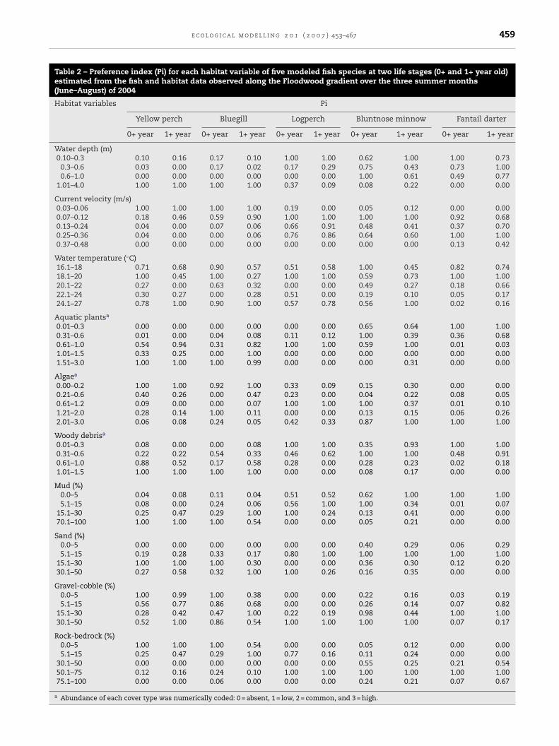

Page 7

e c o l o g i c a l m o d e l l i n g 2 0 1 ( 2 0 0 7 ) 453–467 459

Table 2 – Preference index (Pi) for each habitat variable of five modeled fish species at two life stages (0+ and 1+ year old)estimated from the fish and habitat data observed along the Floodwood gradient over the three summer months(June–August) of 2004

Habitat variables Pi

Yellow perch Bluegill Logperch Bluntnose minnow Fantail darter

0+ year 1+ year 0+ year 1+ year 0+ year 1+ year 0+ year 1+ year 0+ year 1+ year

Water depth (m)0.10–0.3 0.10 0.16 0.17 0.10 1.00 1.00 0.62 1.00 1.00 0.73

0.3–0.6 0.03 0.00 0.17 0.02 0.17 0.29 0.75 0.43 0.73 1.000.6–1.0 0.00 0.00 0.00 0.00 0.00 0.00 1.00 0.61 0.49 0.77

1.01–4.0 1.00 1.00 1.00 1.00 0.37 0.09 0.08 0.22 0.00 0.00

Current velocity (m/s)0.03–0.06 1.00 1.00 1.00 1.00 0.19 0.00 0.05 0.12 0.00 0.000.07–0.12 0.18 0.46 0.59 0.90 1.00 1.00 1.00 1.00 0.92 0.680.13–0.24 0.04 0.00 0.07 0.06 0.66 0.91 0.48 0.41 0.37 0.700.25–0.36 0.04 0.00 0.00 0.06 0.76 0.86 0.64 0.60 1.00 1.000.37–0.48 0.00 0.00 0.00 0.00 0.00 0.00 0.00 0.00 0.13 0.42

Water temperature (◦C)16.1–18 0.71 0.68 0.90 0.57 0.51 0.58 1.00 0.45 0.82 0.7418.1–20 1.00 0.45 1.00 0.27 1.00 1.00 0.59 0.73 1.00 1.0020.1–22 0.27 0.00 0.63 0.32 0.00 0.00 0.49 0.27 0.18 0.6622.1–24 0.30 0.27 0.00 0.28 0.51 0.00 0.19 0.10 0.05 0.1724.1–27 0.78 1.00 0.90 1.00 0.57 0.78 0.56 1.00 0.02 0.16

Aquatic plantsa

0.01–0.3 0.00 0.00 0.00 0.00 0.00 0.00 0.65 0.64 1.00 1.000.31–0.6 0.01 0.00 0.04 0.08 0.11 0.12 1.00 0.39 0.36 0.680.61–1.0 0.54 0.94 0.31 0.82 1.00 1.00 0.59 1.00 0.01 0.031.01–1.5 0.33 0.25 0.00 1.00 0.00 0.00 0.00 0.00 0.00 0.001.51–3.0 1.00 1.00 1.00 0.99 0.00 0.00 0.00 0.31 0.00 0.00

Algaea

0.00–0.2 1.00 1.00 0.92 1.00 0.33 0.09 0.15 0.30 0.00 0.000.21–0.6 0.40 0.26 0.00 0.47 0.23 0.00 0.04 0.22 0.08 0.050.61–1.2 0.09 0.00 0.00 0.07 1.00 1.00 1.00 0.37 0.01 0.101.21–2.0 0.28 0.14 1.00 0.11 0.00 0.00 0.13 0.15 0.06 0.262.01–3.0 0.06 0.08 0.24 0.05 0.42 0.33 0.87 1.00 1.00 1.00

Woody debrisa

0.01–0.3 0.08 0.00 0.00 0.08 1.00 1.00 0.35 0.93 1.00 1.000.31–0.6 0.22 0.22 0.54 0.33 0.46 0.62 1.00 1.00 0.48 0.910.61–1.0 0.88 0.52 0.17 0.58 0.28 0.00 0.28 0.23 0.02 0.181.01–1.5 1.00 1.00 1.00 1.00 0.00 0.00 0.08 0.17 0.00 0.00

Mud (%)0.0–5 0.04 0.08 0.11 0.04 0.51 0.52 0.62 1.00 1.00 1.005.1–15 0.08 0.00 0.24 0.06 0.56 1.00 1.00 0.34 0.01 0.07

15.1–30 0.25 0.47 0.29 1.00 1.00 0.24 0.13 0.41 0.00 0.0070.1–100 1.00 1.00 1.00 0.54 0.00 0.00 0.05 0.21 0.00 0.00

Sand (%)0.0–5 0.00 0.00 0.00 0.00 0.00 0.00 0.40 0.29 0.06 0.295.1–15 0.19 0.28 0.33 0.17 0.80 1.00 1.00 1.00 1.00 1.00

15.1–30 1.00 1.00 1.00 0.30 0.00 0.00 0.36 0.30 0.12 0.2030.1–50 0.27 0.58 0.32 1.00 1.00 0.26 0.16 0.35 0.00 0.00

Gravel-cobble (%)0.0–5 1.00 0.99 1.00 0.38 0.00 0.00 0.22 0.16 0.03 0.195.1–15 0.56 0.77 0.86 0.68 0.00 0.00 0.26 0.14 0.07 0.82

15.1–30 0.28 0.42 0.47 1.00 0.22 0.19 0.98 0.44 1.00 1.0030.1–50 0.52 1.00 0.86 0.54 1.00 1.00 1.00 1.00 0.07 0.17

Rock-bedrock (%)0.0–5 1.00 1.00 1.00 0.54 0.00 0.00 0.05 0.12 0.00 0.005.1–15 0.25 0.47 0.29 1.00 0.77 0.16 0.11 0.24 0.00 0.00

30.1–50 0.00 0.00 0.00 0.00 0.00 0.00 0.55 0.25 0.21 0.5450.1–75 0.12 0.16 0.24 0.10 1.00 1.00 1.00 1.00 1.00 1.0075.1–100 0.00 0.00 0.06 0.00 0.00 0.00 0.24 0.21 0.07 0.67

a Abundance of each cover type was numerically coded: 0 = absent, 1 = low, 2 = common, and 3 = high.

Page 8

460 e c o l o g i c a l m o d e l l i n g 2 0 1 ( 2 0 0 7 ) 453–467

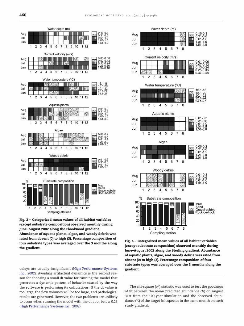
Fig. 3 – Categorized mean values of all habitat variables(except substrate composition) observed monthly duringJune–August 2002 along the Floodwood gradient.Abundance of aquatic plants, algae, and woody debris wasrated from absent (0) to high (3). Percentage composition offour substrate types was averaged over the 3 months along

Fig. 4 – Categorized mean values of all habitat variables(except substrate composition) observed monthly duringJune–August 2002 along the Sterling gradient. Abundanceof aquatic plants, algae, and woody debris was rated fromabsent (0) to high (3). Percentage composition of foursubstrate types was averaged over the 3 months along the

of fit between the mean predicted abundance (%) on August

the gradient.

delays are usually insignificant (High Performance SystemsInc., 2002). Avoiding artifactual dynamics is the second rea-son for choosing a small dt value for running the model thatgenerates a dynamic pattern of behavior caused by the waythe software is performing its calculations. If the dt value istoo large, the flow volumes will be too large, and pathological

results are generated. However, the two problems are unlikelyto occur when running the model with the dt at or below 0.25(High Performance Systems Inc., 2002).

gradient.

The chi-square (�2) statistic was used to test the goodness

31st from the 100-year simulation and the observed abun-dance (%) of the target fish species in the same month on eachstudy gradient.

Page 9

g 2 0

4

4

Ppspig

FeCr

e c o l o g i c a l m o d e l l i n

. Results

.1. Model prediction

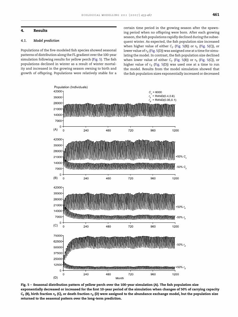
opulations of the five-modeled fish species showed seasonalatterns of distribution along the FL gradient over the 100-year

imulation following results for yellow perch (Fig. 5). The fishopulations declined in winter as a result of winter mortal-

ty and increased in the growing season owning to birth androwth of offspring. Populations were relatively stable for a

ig. 5 – Seasonal distribution pattern of yellow perch over the 10xponentially decreased or increased for the first 10-year period

y (B), birth fraction rb (C), or death fraction rd (D) were assignedeturned to the seasonal pattern over the long-term prediction.

1 ( 2 0 0 7 ) 453–467 461

certain time period in the growing season after the spawn-ing period when no offspring were born. After each growingseason, the fish populations rapidly declined during the subse-quent winter. As expected, the fish population size increasedwhen higher value of either Cy (Fig. 5(B)) or rb (Fig. 5(C)), orlower value of rd (Fig. 5(D)) was assigned one at a time for simu-lating the model. In contrast, the fish population size declined

when lower value of either Cy (Fig. 5(B)) or rb (Fig. 5(C)), orhigher value of rd (Fig. 5(D)) was used one at a time to runthe model. Results from the model simulation showed thatthe fish population sizes exponentially increased or decreased

0-year simulation (A). The fish population sizeof the simulation when changes of 50% of carrying capacityto the abundance exchange model, but the population size

Page 10

462 e c o l o g i c a l m o d e l l i n g

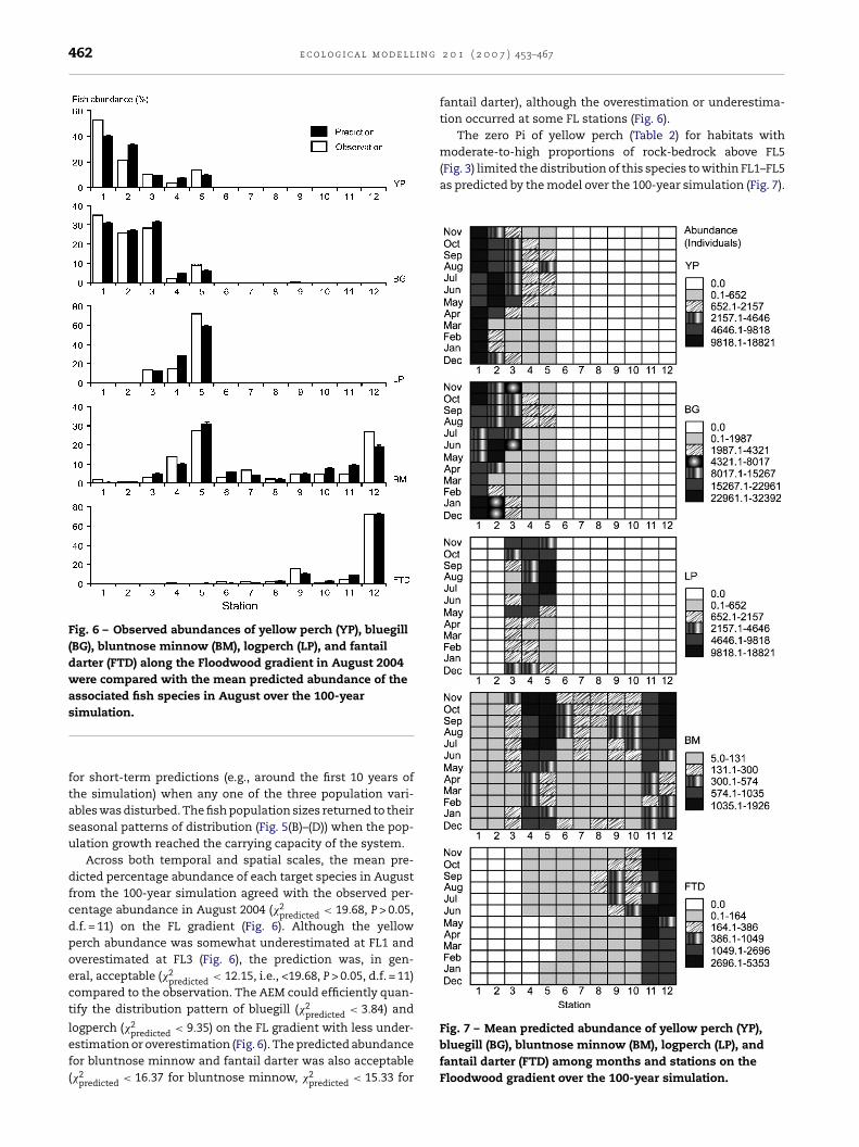
Fig. 6 – Observed abundances of yellow perch (YP), bluegill(BG), bluntnose minnow (BM), logperch (LP), and fantaildarter (FTD) along the Floodwood gradient in August 2004were compared with the mean predicted abundance of theassociated fish species in August over the 100-year

moderate-to-high proportions of rock-bedrock above FL5(Fig. 3) limited the distribution of this species to within FL1–FL5as predicted by the model over the 100-year simulation (Fig. 7).

Fig. 7 – Mean predicted abundance of yellow perch (YP),

simulation.

for short-term predictions (e.g., around the first 10 years ofthe simulation) when any one of the three population vari-ables was disturbed. The fish population sizes returned to theirseasonal patterns of distribution (Fig. 5(B)–(D)) when the pop-ulation growth reached the carrying capacity of the system.

Across both temporal and spatial scales, the mean pre-dicted percentage abundance of each target species in Augustfrom the 100-year simulation agreed with the observed per-centage abundance in August 2004 (�2

predicted < 19.68, P > 0.05,d.f. = 11) on the FL gradient (Fig. 6). Although the yellowperch abundance was somewhat underestimated at FL1 andoverestimated at FL3 (Fig. 6), the prediction was, in gen-eral, acceptable (�2

predicted < 12.15, i.e., <19.68, P > 0.05, d.f. = 11)compared to the observation. The AEM could efficiently quan-tify the distribution pattern of bluegill (�2

predicted < 3.84) and

logperch (�2 < 9.35) on the FL gradient with less under-

predictedestimation or overestimation (Fig. 6). The predicted abundancefor bluntnose minnow and fantail darter was also acceptable(�2

predicted < 16.37 for bluntnose minnow, �2predicted < 15.33 for

2 0 1 ( 2 0 0 7 ) 453–467

fantail darter), although the overestimation or underestima-tion occurred at some FL stations (Fig. 6).

The zero Pi of yellow perch (Table 2) for habitats with

bluegill (BG), bluntnose minnow (BM), logperch (LP), andfantail darter (FTD) among months and stations on theFloodwood gradient over the 100-year simulation.

Page 11

g 2 0 1 ( 2 0 0 7 ) 453–467 463

TiJg(oaJst

prbmagRi(rsdF

4

TFt2a(daSdPfSs(co(Su(

a(aewtdMdao

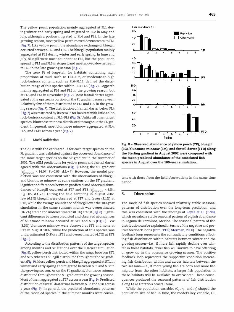
Fig. 8 – Observed abundance of yellow perch (YP), bluegill(BG), bluntnose minnow (BM), and fantail darter (FTD) alongthe Sterling gradient in August 2002 were compared with

e c o l o g i c a l m o d e l l i n

he yellow perch population mainly aggregated at FL1 dur-ng winter and early spring and migrated to FL2 in May anduly, although a portion migrated to FL4 and FL5. In the laterowing season, most yellow perch moved downstream to FL1Fig. 7). Like yellow perch, the abundance exchange of bluegillccurred between FL1 and FL5. The bluegill population mainlyggregated at FL1 during winter and early spring. In June anduly, bluegill were most abundant at FL2, but the populationpread to FL1 and FL3 in August, and most moved downstreamo FL1 in the late growing season (Fig. 7).

The zero Pi of logperch for habitats containing highroportions of mud, such as FL1–FL2, or moderate-to-highock-bedrock content, such as FL6–FL12, defined the distri-ution range of this species within FL3–FL5 (Fig. 7). Logperchainly aggregated at FL4 and FL5 in the growing season, but

t FL3 and FL4 in November (Fig. 7). Most fantail darter aggre-ated at the upstream portion on the FL gradient across a year.elatively few of them distributed to FL4 and FL5 in the grow-

ng season (Fig. 7). The distribution of fantail darter below FL4Fig. 7) was restricted by its zero Pi for habitats with little-to-noock-bedrock content at FL1–FL3 (Fig. 3). Unlike all other targetpecies, bluntnose minnow distributed throughout the FL gra-ient. In general, most bluntnose minnow aggregated at FL4,L5, and FL12 across a year (Fig. 7).

.2. Model validation

he AEM with the estimated Pi for each target species on theL gradient was validated against the observed abundance ofhe same target species on the ST gradient in the summer of002. The AEM predictions for yellow perch and fantail dartergreed with the observations (Fig. 8) along the ST gradient�2

predicted < 14.07, P > 0.05, d.f. = 7). However, the model pre-iction was not consistent with the observations of bluegillnd bluntnose minnow at some stations on the ST gradient.ignificant differences between predicted and observed abun-ances of bluegill occurred at ST7 and ST8 (�2

predicted < 3.84,≤ 0.05, d.f. = 1). During the field sampling in August 2002,

ew (6.3%) bluegill were observed at ST7 and fewer (3.1%) atT8, while the average abundance of bluegill over the 100-yearimulation in the same summer month was overestimated16.2%) at ST7 and underestimated (0.3%) at ST8 (Fig. 8). Signifi-ant differences between predicted and observed abundancesf bluntnose minnow occurred at ST1 and ST3 (Fig. 8). Few

3.5%) bluntnose minnow were observed at ST1 and none atT3 in August 2002, while the prediction of this species wasnderestimated (0.3%) at ST1 and overestimated (4.7%) at ST3

Fig. 8).According to the distribution patterns of the target species

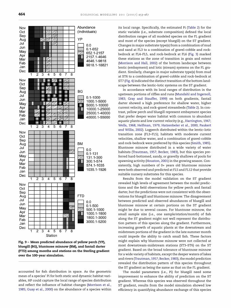
mong months and ST stations over the 100-year simulationFig. 9), yellow perch distributed within the range between ST1nd ST6, whereas bluegill distributed throughout the ST gradi-nt (Fig. 9). Most yellow perch and bluegill aggregated at ST1 ininter and early spring and migrated between ST1 and ST2 in

he growing season. As on the FL gradient, bluntnose minnowistributed throughout the ST gradient in the growing season.

ost of them aggregated at ST7 across a year (Fig. 9). Predicted

istribution of fantail darter was between ST7 and ST8 acrossyear (Fig. 9). In general, the predicted abundance patterns

f the modeled species in the summer months were consis-

the mean predicted abundance of the associated fishspecies in August over the 100-year simulation.

tent with those from the field observations in the same timeperiod.

5. Discussion

The modeled fish species showed relatively stable seasonalpatterns of distribution over the long-term prediction, andthis was consistent with the findings of Reyes et al. (1994),which revealed a stable seasonal pattern of pigfish abundancein Laguna de Terminos, Mexico. The seasonal pattern of fishdistribution can be explained in terms of the negative and pos-itive feedback loops (Ford, 1999; Sterman, 2000). The negativefeedback loop represents the contradictory conditions affect-ing fish distribution within habitats between winter and thegrowing season—i.e., if more fish rapidly decline over win-ter in these habitats, fewer fish will survive to have offspringor grow up in the successive growing season. The positivefeedback loop represents the supportive condition increas-ing fish distribution within and across habitats between thetwo seasons—i.e., if more young fish are born and more fishmigrate from the other habitats, a larger fish population inthese habitats will be available to overwinter. These conse-

quences produced the seasonal patterns of fish distributionalong Lake Ontario’s coastal zone.

While the population variables (Cy, rb, and rd) shaped thepopulation size of fish in time, the model’s key variable, HP,

Page 12

464 e c o l o g i c a l m o d e l l i n g

Fig. 9 – Mean predicted abundance of yellow perch (YP),bluegill (BG), bluntnose minnow (BM), and fantail darter(FTD) among months and stations on the Sterling gradient

over the 100-year simulation.

accounted for fish distribution in space. As the geometric

mean of a species’ Pi for both static and dynamic habitat vari-ables, HP could capture the local range of species distributionand reflect the influence of habitat changes (Morrison et al.,1985; Guay et al., 2000) on the abundance of a species within

2 0 1 ( 2 0 0 7 ) 453–467

its local range. Specifically, the estimated Pi (Table 2) for thestatic variable (i.e., substrate composition) defined the localdistribution ranges of all modeled species on the FL gradientand most of the species (except bluegill) on the ST gradient.Changes in major substrate type(s) from a combination of mudand sand at FL3 to a combination of gravel-cobble and rock-bedrock at FL4–FL5, and rock-bedrock at FL6 (Fig. 3) markedthese stations as the zone of transition in grain and extent(Morrison and Hall, 2002) of the bottom landscape betweenlentic (embayment) and lotic (stream) systems on the FL gra-dient. Similarly, changes in major substrate type(s) from mudat ST6 to a combination of gravel-cobble and rock-bedrock atST7 (Fig. 4) indicated the distinct transition of the bottom land-scape between the lentic–lotic systems on the ST gradient.

In accordance with its local ranges of distribution in theupstream portions of riffles and runs (Mundahl and Ingersoll,1983; Gray and Stauffer, 1999) on both gradients, fantaildarter showed a high preference for shallow water, highercurrent velocity, and rock–gravel streambeds (Table 2). In con-trast, yellow perch and bluegill represent embayment speciesthat prefer deeper water habitat with common to abundantaquatic plants and low current velocity (e.g., Harrington, 1947;Wells, 1968; Helfman, 1979; Hatzenbeler et al., 2000; Paukertand Willis, 2002). Logperch distributed within the lentic–lotictransition zone (FL3–FL5); habitats with moderate currentvelocities, shallow water, and a combination of gravel-cobbleand rock-bedrock were preferred by this species (Smith, 1985).Bluntnose minnow distributed in a wide variety of waterhabitats (Trautman, 1957; Becker, 1983), but this species pre-ferred hard-bottomed, sandy, or gravelly shallows of pools forspawning activity (Houston, 2001) in the growing season. Con-sistently, high numbers of 0+ years old bluntnose minnowwere both observed and predicted at FL5 and FL12 that providesuitable nursery substrates for this species.

Results from the model validation on the ST gradientrevealed high levels of agreement between the model predic-tions and the field observations for yellow perch and fantaildarter, but the predictions were not consistent with the obser-vations for bluegill and bluntnose minnow. The disagreementbetween predicted and observed abundances of bluegill andbluntnose minnow at certain portions on the ST gradientmight be due to several causes. For bluntnose minnow, thesmall sample size (i.e., one sample/station/month) of fishalong the ST gradient might not well represent the distribu-tion pattern of this species along the gradient. Furthermore,increasing growth of aquatic plants at the downstream andmidstream portions of the gradient in the late summer monthcould impede the ability to catch small fish. These factorsmight explain why bluntnose minnow were not collected atmost downstream-midstream stations (ST3–ST6) on the STgradient. Based on the broad tolerance of bluntnose minnowfor a wide variety of habitats, except the deeper waters of lakesand rivers (Trautman, 1957; Becker, 1983), the model predictionrevealed the distribution pattern of this species throughoutthe ST gradient as being the same as that on the FL gradient.

The model parameters (i.e., Pi) for bluegill need some

improvement to enhance the ability of prediction on the STgradient. Whereas this species was observed throughout theST gradient, results from the model simulation showed lowefficiency in quantifying abundance exchange of this species

Page 13

g 2 0

i(iPiatsh

finwSfettlrpvmo

gcNdsbtnvbsFddwtde

woemmcte

A

Tite

r

e c o l o g i c a l m o d e l l i n

n the upstream portion of the gradient. Pajak and Neves1987) proposed three primary concerns that are generallymplicit in model validation procedures based on fish speciesi; one has to ensure that (1) the fish species data to be val-dated are accurately collected, (2) the habitat condition isccurately measured, and it is limited primarily by the habi-at variables included in the model, and (3) the samplingites are representative sub-samples of the target fish species’abitats.

In this study, it is believed that methods of collecting bothsh and habitat data were appropriate. Nevertheless, it wasoticeable that the sampling sites on the FL gradient might notell represent all kinds of utilized substrates for bluegill on theT gradient. While the Pi for the rest of the habitat variablesell within the observed ranges for bluegill on both study gradi-nts, the Pi for substrate variables showed some gaps betweenhe quantified intervals (Table 2). This observation indicateshat although the substrates along the FL gradient were col-ected at a fine scale (900 samples), they were still unable toepresent diverse proportions of the bottom substrates occu-ied by bluegill on the ST gradient. Thus, the Pi for substrateariables for this species may need to be improved for betterodel prediction. Similar gaps in sampling coverage did not

ccur for the other modeled species.Results from this study suggest that the species’ Pi for a

iven habitat variable estimated from one study area may notompletely represent its Pi in another study area (Pajak andeves, 1987; O’Connor, 2002). Thus, to apply the AEM for pre-icting fish species distribution in other water systems, onehould crosscheck the fish species’ Pi from existing data atoth local and regional scales before incorporating them intohe AEM for computing the species’ HP. This is particularlyecessary for fish species with broad tolerances on the habitatariables that can powerfully define local ranges of fish distri-ution (Hatzenbeler et al., 2000) or control distribution of fishpecies from cell to cell (e.g., substrate types; Reyes et al., 1994).or different water systems with different environmental con-itions, influential habitat variables should be considered foreveloping fish species Pi. Additionally, in large water systemshere fish movements in both vertical and horizontal direc-

ions are equally important, two or more dimensions of fishistribution may need to be added in the model (e.g., Morrisont al., 1985; Reyes et al., 1994).

Overall, the AEM empirically developed from the field-ork data performs rather well for quantifying distributionsf the coastal fish species assemblages along Lake Ontario’smbayment–tributary stream gradients. With its flexibleodel structure that can accommodate array functions andultiple differential equations for both static and dynamic

omponents, the AEM can be modified to determine dis-ribution patterns of other types of organisms in differentnvironmental and geographic systems.

cknowledgments

his study was supported by the Lake Ontario Biocomplex-ty Project (Natural Science Foundation OCE-0083625) andhe Royal Thai Government. I thank two anonymous review-rs for providing instructive suggestions to greatly improve

1 ( 2 0 0 7 ) 453–467 465

the manuscript, and Mark B. Bain, Patrick J. Sullivan, andDaniel P. Loucks for their comments on this work. I thankKathy Mills, Carol Steinhart, Dolina Millar, Kristi Arend, andGeoff Steinhart for their help in the process of manuscriptpreparation.

e f e r e n c e s

Becker, G.C., 1983. Fishes of Wisconsin. University of WisconsinPress, Madison, 1052 pp.

Bovee, K.D., 1982. A Guide to Stream Habitat Analysis using TheInstream Flow Incremental Methodology. Instream FlowInformation Paper 5: FWS/OBS–82/26. U.S. Fish and WildlifeService.

Bovee, K.D., 1986. Development and Evaluation of HabitatSuitability Criteria for Use in The Instream Flow IncrementalMethodology. Instream Flow Information Paper 21: 86(7). U.S.Fish and Wildlife Service.

Cadenasso, M.L., Pickett, S.T.A., Weathers, K.C., Jones, C.G., 2003.A framework for a theory of ecological boundaries. BioScience53, 750–758.

Clements, F.E., 1905. Research Methods in Ecology. UniversityPublishing Company, Nebraska, 334 pp.

Degraaf, D.A., Bain, L.H., 1986. Habitat use by and preferences ofjuvenile Atlantic salmon in two Newfoundland Rivers. Trans.Am. Fish. Soc. 115, 671–681.

Dew, I.M., 2001. Theoretical model of a new fishery under asimple quota management system. Ecol. Model. 143, 59–70.

Elith, J., Burgman, M., 2002. Predictions and their validation: rareplants in Central Highlands, Victoria, Australia. In: Scott, J.M.,Heglund, P.J., Morrison, M.L., Haufler, J.B., Raphael, M.G., Wall,W.A., Samson, F.B. (Eds.), Predicting Species Occurrences:Issues of Accuracy and Scale. Island Press, Washington, pp.303–313.

Fagan, W.F., Cantrell, R.S., Cosner, C., 1999. How habitat edgeschange species interactions. Am. Nat. 153, 165–182.

Fielding, A.H., 2002. What are appropriate characteristics of anaccuracy measure? In: Scott, J.M., Heglund, P.J., Morrison, M.L.,Haufler, J.B., Raphael, M.G., Wall, W.A., Samson, F.B. (Eds.),Predicting Species Occurrences: Issues of Accuracy and Scale.Island Press, Washington, pp. 271–280.

Fischer, H.B., List, E.J., Koh, R.C.Y., Imberger, J., Brooks, N.H., 1979.Mixing in Inland and Coastal Waters. Academic Press, SanDiego, California, 483 pp.

Ford, A., 1999. Modeling the Environment: An Introduction toSystem Dynamics Modeling of Environmental Systems. IslandPress, Washington, DC, 401 pp.

Fortin, M.J., Olson, R.J., Ferson, S., Iverson, L., Hunsaker, C.,Edwards, G., Levine, D., Butera, K., Klemas, V., 2000. Issuesrelated to the detection of boundaries. Landsc. Ecol. 15,453–466.

Gaff, H., DeAngelis, D.L., Gross, L.J., Salinas, R., 2000. A dynamiclandscape model for fish in the Everglades and its applicationto restoration. Ecol. Model. 127, 33–52.

Gertseva, V.V., Gertsev, V.I., Ponomarev, N.Y., 2003.Tropho-ethological polymorphism of fish as a strategy ofhabitat development: a simulation model. Ecol. Model. 167,159–164.

Gertseva, V.V., Schindler, J.E., Gertsev, V.I., Ponomarev, N.Y.,English, W.R., 2004. A simulation model of the dynamics ofaquatic macroinvertebrate communities. Ecol. Model. 176,

173–186.

Gottlieb, S.J., 1998. Nutrient removal by age-0 Atlantic menhaden(Brevoortia tyrranus) in Chesapeake Bay and implications forseasonal management of the fishery. Ecol. Model. 112,111–130.

Page 14

i n g

466 e c o l o g i c a l m o d e l l

Gray, E.V.S., Stauffer Jr., J.R., 1999. Comparative microhabitat useof ecologically similar benthic fishes. Environ. Biol. Fish. 56,443–453.

Guay, J.C., Boisclair, D., Rioux, D., Leclerc, M., Lapointe, M.,Legendre, P., 2000. Development and validation of numericalhabitat models for juveniles of Atlantic salmon (Salmo salar).Can. J. Fish. Aquat. Sci. 57, 2065–2075.

Guisan, A., Zimmermann, N.E., 2000. Predictive habitatdistribution models in ecology. Ecol. Model. 135,147–186.

Haefner, J.W., 1996. Modeling Biological Systems: Principles andApplications. Chapman & Hall, New York, 473 pp.

Harding, E.K., 2002. Modelling the influence of seasonalinter-habitat movements by an ecotone rodent. Biol. Conserv.104, 227–237.

Harrington Jr., R.W., 1947. Observations on the breeding habits ofthe yellow perch, Perca flavescens (Mitchill). Copeia 1947,199–200.

Hatzenbeler, G.R., Bozek, M.A., Jennings, M.J., Emmons, E.E., 2000.Seasonal variation in fish assemblage structure and habitatstructure in the nearshore littoral zone of Wisconsin Lakes. N.Am. J. Fish. Manage. 20, 360–368.

Helfman, G.S., 1979. Twilight activities of yellow perch, Percaflavescens. J. Fish. Res. Board Can. 36, 173–179.

High Performance Systems Inc., 2002. STELLA® Research, Version7.0.3 for Windows. Hanover, NH.

Houston, J., 2001. Status of the bluntnose minnow, Pimephalesnotatus, in Canada. Can. Field Nat. 115, 145–151.

Johnson, A.R., Wiens, J.A., Milne, B.T., Crist, T.O., 1992. Animalmovements and population dynamics in heterogeneouslandscapes. Landsc. Ecol. 7, 63–75.

Kilpatrick, H.J., LaBonte, A.M., Barclay, J.S., Warner, G., 2004.Assessing strategies to improve bowhunting as an urban deermanagement tool. Wildl. Soc. B 32, 1177–1184.

Kot, M., 2001. Elements of Mathematical Ecology. CambrideUniversity Press, Cambridge, 453 pp.

Krivtsov, V., Corliss, J., Bellinger, E., Sigee, D., 2000. Indirectregulation rule for consecutive stages of ecologicalsuccession. Ecol. Model. 133, 73–81.

Kupschus, S., 2003. Development and evaluation of statisticalhabitat suitability models: and example based on juvenilespotted seatrout Cynoscion nebulosus. Mar. Ecol. Prog. Ser. 265,197–212.

Leopold, A., 1933. Game Management. Charles Scribner’s Sons,New York, 481 pp.

Lewis, M.A., 1997. Variability, patchiness, and jump dispersal inthe spread of an invading population. In: Tilman, D., Kareiva,P. (Eds.), Spatial Ecology: The Role of Space in PopulationDynamics and Interspecific Interactions. Princeton UniversityPress, New Jersey, pp. 46–69.

Lidicker, W.Z.J., 1999. Responses of mammals to habitat edges: anoverview. Landsc. Ecol. 14, 333–343.

Lucas, M.C., Baras, E., 2001. Migration of Freshwater Fishes.Blackwell Science, London, 420 pp.

Marın, V.H., 1997. A simple-biology, stage-structured populationmodel of the spring dynamics of Calanus chilensis at Mejillonesdel Sur Bay, Chile. Ecol. Model. 105, 65–82.

Martino, E.J., Able, K.W., 2003. Fish assemblages across themarine to low salinity transition zone of a temperate estuary.Estuar. Coast. Shelf S. 56, 969–987.

McCausland, W.D., Mente, E., Pierce, G.J., Theodossiou, I., 2006. Asimulation model of sustainability of coastal communities:aquaculture, fishing, environment and labour markets. Ecol.Model. 193, 271–294.

Miller, B.A., Sadro, S., 2003. Residence time and seasonalmovements of juvenile coho salmon in the ecotone and lowerestuary of Winchester Creek, South Slough, Oregon. Trans.Am. Fish. Soc. 132, 546–559.

2 0 1 ( 2 0 0 7 ) 453–467

Morrison, K.A., Therien, N., Coupal, B., 1985. Simulating fishredistribution in the LG-2 reservoir after flooding. Ecol. Model.28, 97–111.

Morrison, M.L., Hall, L.S., 2002. Standard terminology: toward acommon language to advance ecological understanding andapplication. In: Scott, J.M., Heglund, P.J., Morrison, M.L.,Haufler, J.B., Raphael, M.G., Wall, W.A., Samson, F.B. (Eds.),Predicting Species Occurrences: Issues of Accuracy and Scale.Island Press, Washington, pp. 43–52.

Mundahl, N.D., Ingersoll, C.G., 1983. Early autumn movementsand densities of johny (Etheostoma nigrum) and fantail (E.flabellare) darters in a southwestern Ohio stream. Ohio J. Sci.83, 103–108.

Nisbet, R.M., Gurney, W.S.C., 1982. Modelling FluctuatingPopulations. John Wiley & Son, New York, 379 pp.

O’Connor, R.J., 2002. The conceptual basis of species distributionmodeling: time for a paradigm shift? In: Scott, J.M., Heglund,P.J., Morrison, M.L., Haufler, J.B., Raphael, M.G., Wall, W.A.,Samson, F.B. (Eds.), Predicting Species Occurrences: Issues ofAccuracy and Scale. Island Press, Washington, pp. 25–33.

Odum, E.P., 1971. Fundamentals of Ecology, 3rd ed. W.B. SaundersCompany, Philadelphia, 574 pp.

Okubo, A., Levin, S.A. (Eds.), 2001. Diffusion and EcologicalProblems: Modern Perspectives. Springer, New York, p. 467.

Olden, J.D., Jackson, D.A., Peres-Neto, P.R., 2002. Predictive modelsof fish species distributions: a note on proper validation andchance predictions. Trans. Am. Fish. Soc. 131, 329–336.

Ottaviani, D., Lasinio, G.J., Boitani, L., 2004. Two statisticalmethods to validate habitat suitability models usingpresence-only data. Ecol. Model. 179, 417–443.

Pajak, P., Neves, R.J., 1987. Habitat suitability and fish production:a model evaluation for rock bass in two Virginia streams.Trans. Am. Fish. Soc. 116, 839–850.

Pan, Y., Raynal, D.J., 1995. Decomposing tree annual volumeincrements and constructing a system dynamic model of treegrowth. Ecol. Model. 82, 299–312.

Paukert, C.P., Willis, D.W., 2002. Seasonal and diel habitatselection by bluegills in a shallow natural lake. Trans. Am.Fish. Soc. 131, 1131–1139.

Pusey, B., Arthington, A.H., Read, M.G., 1993. Spatial and temporalvariation in fish assemblage structure in the Mary River,south-eastern Queensland: the influence of habitat structure.Environ. Biol. Fish. 37, 355–380.

Reyes, E., Sklar, F.H., Day, J.W., 1994. A regional organism exchangemodel for simulating fish migration. Ecol. Model. 74, 255–276.

Ries, L., Fletcher Jr., R.J., Battin, J., Sisk, T.D., 2004. Ecologicalresponses to habitat edges: mechanisms, models, andvariability explained. Annu. Rev. Ecol. Evol. Syst. 35, 491–522.

Risser, P.G., 1990. The ecological importance of land–waterecotones. In: Naiman, R.J., Decamps, H. (Eds.), The Ecologyand Management of Aquatic–Terrestrial Ecotones. ParthenonPublishing Group, France, pp. 7–21.

Skalski, G.T., Gilliam, J.E., 2000. Modeling diffusive spread in aheterogeneous population: a movement study with streamfish. Ecology 81, 1685–1700.

Smith, C.L., 1985. The Inland Fishes of New York State. New YorkState Department of Environmental Conservation, New York,522 pp.

Sterman, J.D., 2000. Business Dynamics: Systems Thinking andModeling for a Complex World. McGraw-Hill, Singapore, 982pp.

Sparrevohn, C.R., Nielsen, A., Stottrup, J.G., 2002. Diffusion of fishfrom a single release point. Can. J. Fish. Aquat. Sci. 59, 844–853.

Tilman, D., Kareiva, P. (Eds.), 1997. Spatial Ecology: The Role of

Space in Population Dynamics and Interspecific Interaction.Princeton University Press, New Jersey, p. 368.

Trautman, M.B., 1957. The Fishes of Ohio. Ohio State UniversityPress, Ohio, 683 pp.

Page 15

g 2 0

T

W

W

e c o l o g i c a l m o d e l l i n

urchin, P., 1998. Quantitative Analysis of Movement: Measuringand Modeling Population Redistribution in Animals andPlants. Sinauer Associates Inc., Massachusetts, 396 pp.

ells, L., 1968. Seasonal depth distribution of fish insoutheastern Lake Michigan. Fisheries Bulletin, vol. 67. U.S.Fish and Wildlife Service.

hittaker, R.H., 1975. Communities and Ecosystem, 2nd ed.Macmillan Publishing, New York, 385 pp.

1 ( 2 0 0 7 ) 453–467 467

Wiens, J.A., 2002. Riverine landscapes: taking landscape ecologyinto the water. Freshwater Biol. 47, 501–515.

Willis, T.V., Magnuson, J.J., 2002. Patterns in fish species

composition across the interface between streams and lakes.Can. J. Fish. Aquat. Sci. 57, 1042–1052.

Winemiller, K.O., Leslie, M.A., 1992. Fish assemblages across acomplex, tropical freshwater/marine ecotone. Environ. Biol.Fish. 34, 29–50.