AMSSpin: A LabVIEW program for measuring the anisotropy of magnetic susceptibility with the Kappabridge KLY-4S

AMSSpin: A LabVIEW program for measuring theanisotropy of magnetic susceptibility with the KappabridgeKLY-4S

Jeffrey S. Gee and Lisa TauxeGeosciences Research Division, Scripps Institution of Oceanography, University of California, San Diego, La Jolla,California 92093-0220, USA ([email protected])

Cathy ConstableInstitute of Geophysics and Planetary Physics, Scripps Institution of Oceanography, University of California, San Diego,La Jolla, California 92093-0225, USA

[1] Anisotropy of magnetic susceptibility (AMS) data are widely used as a petrofabric tool because thetechnique is rapid and nondestructive and because static measurement systems are capable of determiningsmall degrees of anisotropy. The Kappabridge KLY-4S provides high resolution as a result of the largenumber of measurements acquired while rotating the sample about three orthogonal axes. Here we describea graphical-based program called AMSSpin for acquiring AMS data with this instrument as well as amodified specimen holder that should further enhance the utility of this instrument. We also outline amethod for analysis of the data (that differs in several ways from that of the software supplied with theinstrument) and demonstrate that the measurement errors are suitable for using linear perturbation analysisto statistically characterize the results. Differences in the susceptibility tensors determined by our newprogram and the SUFAR program supplied with the instrument are small, typically less than or comparableto deviations between multiple measurements of the same specimen.

Components: 6177 words, 13 figures.

Keywords: magnetic fabric; AMS; susceptibility tensor; Kappabridge.

Index Terms: 1518 Geomagnetism and Paleomagnetism: Magnetic fabrics and anisotropy; 1594 Geomagnetism and

Paleomagnetism: Instruments and techniques.

Received 4 February 2008; Revised 17 June 2008; Accepted 27 June 2008; Published 9 August 2008.

Gee, J. S., L. Tauxe, and C. Constable (2008), AMSSpin: A LabVIEW program for measuring the anisotropy of magnetic

susceptibility with the Kappabridge KLY-4S, Geochem. Geophys. Geosyst., 9, Q08Y02, doi:10.1029/2008GC001976.

————————————

Theme: Advances in Instrumentation for Paleomagnetism and Rock MagnetismGuest Editor: V. Salters

1. Introduction

[2] The magnetic fabric of rocks, as quantified byanisotropy of magnetic susceptibility (AMS) meas-

urements, has been used as a petrofabric proxy in awide variety of geological applications (seereviews by Rochette et al. [1992] and Tarlingand Hrouda [1993]). Magnetic susceptibility data

G3G3GeochemistryGeophysics

Geosystems

Published by AGU and the Geochemical Society

AN ELECTRONIC JOURNAL OF THE EARTH SCIENCES

GeochemistryGeophysics

Geosystems

Technical Brief

Volume 9, Number 8

9 August 2008

Q08Y02, doi:10.1029/2008GC001976

ISSN: 1525-2027

Copyright 2008 by the American Geophysical Union 1 of 13

provide a rapid, nondestructive means of charac-terizing the volumetric preferred alignment ofmagnetic phases with sufficient precision to recog-nize very slight degrees of anisotropy (<1%) thatare difficult to quantify with other techniques. Therecently developed Kappabridge KLY-4S and ear-lier KLY-3S [Jelinek and Pokorny, 1997; Pokornyet al., 2004] allow even higher precision determi-nation of the magnetic susceptibility tensor byacquiring substantially more susceptibility data asthe sample is rotated in three orthogonal planes.

[3] We describe here a new program calledAMSSpin for acquiring AMS data from theKappabridge KLY-4S. AMSSpin is designed toprovide a user friendly environment for perhapsthe most common type of measurement (AMS)made with the Kappabridge; other useful featuresof the instrument (e.g., temperature-dependentmeasurements) are not incorporated into our pro-gram. The principal advantages of the programare the real time display of susceptibility dataacquired during a spin (we use the term spin toindicate data from multiple revolutions) and thedisplay of best fit 2-D and 3-D models to the dataas well as the resulting residuals. These data allowthe user to evaluate instrument drift and thesignal-to-noise ratio and to identify some errorsresulting from misorientation or poor centering ofthe specimen. Eigenvectors for the current speci-men can be plotted together with previouslymeasured data (in a variety of coordinate systems)to allow evaluation of within site consistency. Theprocessing of data differs from that of the SUFARprogram supplied with the instrument, which isbased on the Jelinek theory [Jelinek, 1995] ofmeasuring the AMS of a slowly spinning speci-men, both in terms of analyzing data from one

spin as well as in the determination of the sixindependent elements of the best fit tensor. Differ-ences in the susceptibility tensors determined byour new program and the SUFAR program sup-plied with the instrument are small, typically lessthan or comparable to deviations between multi-ple measurements of the same specimen. Finally,we have designed a cubic sample holder for coresamples that allows more reproducible positioningof the sample in three orthogonal orientations(Appendix A).

2. Theory

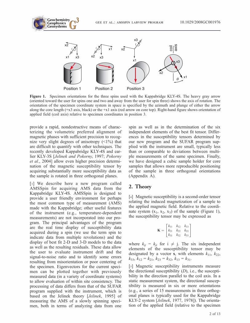
[4] Magnetic susceptibility is a second-order tensorrelating the induced magnetization of a sample tothe applied magnetic field. Relative to the coordi-nate system (x1, x2, x3) of the sample (Figure 1),the susceptibility tensor may be expressed as

K ¼k11 k12 k13k21 k22 k23k31 k32 k33

24

35

where kij = kji for i 6¼ j. The six independentelements of the susceptibility tensor may bedesignated by a vector s, with elements k11, k22,k33, k12 = k21, k23 = k32, k13 = k31.

[5] Magnetic susceptibility instruments measurethe directional susceptibility (D), i.e., the suscepti-bility in the direction parallel to the coil axis. In astatic measurement system, the directional suscep-tibility is measured in six or more orientations(e.g., a series of 15 measurements in three orthog-onal planes is typically used for the KappabridgeKLY-2 system [Jelinek, 1977, 1978]). The orienta-tion of the applied field (relative to the specimen

Figure 1. Specimen orientations for the three spins used with the Kappabridge KLY-4S. The heavy gray arrow(oriented toward the user for spins one and two and away from the user for spin three) shows the axis of rotation. Theorientation of the specimen coordinate system in space is specified by the azimuth and plunge of either the arrowalong the core length (+x3 axis, black) or the +x1 axis (red arrow on core top). Right-hand figure shows orientation ofapplied field (coil axis) relative to specimen coordinates in position 3.

GeochemistryGeophysicsGeosystems G3G3

gee et al.: amsspin labview program 10.1029/2008GC001976

2 of 13

coordinate system) for each of these n measure-ments is described by an n � 6 matrix termed thedesign matrix (A). The n directional susceptibilityvalues (D) are related to the design matrix and s by

D ¼ As ð1Þ

and the best fit values (s) of s in a least squaressense may be calculated from

�s ¼ ATA� ��1

ATD ð2Þ

The best fit values may, in turn, be used to estimateresiduals (di) for each of the measurements.

di ¼ Di � Aijsj ð3Þ

In a slowly spinning specimen measurementsystem such as the Kappabridge KLY-4S, direc-tional susceptibility can be measured as thespecimen is rotated in each of three orthogonalplanes [see Jelinek, 1995], clockwise about the +x1axis, clockwise about the +x2 axis and counter-clockwise about the +x3 axis (Figure 1). Thedirectional susceptibility signal as the specimen isrotated about the +x1 axis (D

x1) is given by

Dx1 ¼ 0 sin qð Þ cos qð Þ½ �k11 k12 k13k12 k22 k23k13 k23 k33

24

35

0

sin qð Þcos qð Þ

24

35

where q is the angle of the applied field relative tothe sample coordinate system. Directional suscept-ibility values are recorded for 64 positions duringeach revolution, and the value for the ith angularmeasurement about the +x1 axis is given by

Dx1i ¼ k22 sin

2 qið Þ þ 2k23 cos qið Þ sin qið Þ þ k33 cos2 qið Þ

We will refer to this as the 2-D model thatdescribes the directional susceptibility duringrotation about one of the sample coordinate axes.Combining three such models (one from rotationabout each of the sample coordinate axes) allows

calculation of a 3-D model. In a similar fashion, thevalues for the ith angular measurement about the+x2 and +x3 axes are given by

Dx2i ¼ k11 sin

2 qið Þ � 2k13 cos qið Þ sin qið Þ þ k33 cos2 qið Þ

Dx3i ¼ k22 sin

2 qið Þ þ 2k12 cos qið Þ sin qið Þ þ k11 cos2 qið Þ

By analogy with (1) above for the static measure-ment system, the 192 directional susceptibilityvalues acquired during these three spins are relatedto the six independent elements of the suscept-ibility tensor by a 192 � 6 design matrix (A):

A ¼

0 sin2 q1ð Þ cos2 q1ð Þ 0 2 cos q1ð Þsin q1ð Þ 0

..

. ... ..

. ... ..

. ...

0 sin2 q64ð Þ cos2 q64ð Þ 0 2 cos q64ð Þsin q64ð Þ 0

sin2 q1ð Þ 0 cos2 q1ð Þ 0 0 �2 cos q1ð Þsin q1ð Þ... ..

. ... ..

. ... ..

.

sin2 q64ð Þ 0 cos2 q64ð Þ 0 0 �2 cos q64ð Þsin q64ð Þcos2 q1ð Þ sin2 q1ð Þ 0 2 cos q1ð Þsin q1ð Þ 0 0

..

. ... ..

. ... ..

. ...

cos2 q64ð Þ sin2 q64ð Þ 0 2 cos q64ð Þsin q64ð Þ 0 0

26666666666666664

37777777777777775

where the first 64 rows refer to rotations about the+x1 axis, the middle 64 rows refer to rotationsabout the +x2 axis and the final 64 rows refer torotations about the +x3 axis.

[6] In practice, there are several additional consid-erations involved in assembling the array of 192directional susceptibility values to be used inconjunction with the design matrix in estimatingthe elements of s. First, the directional susceptibil-ity values are subject to a phase lag (typically�20�) imparted by the finite response time of theelectronics. This phase angle is determined bymeasurement of an axial standard and applied toall subsequent data. Second, the directional sus-ceptibility values measured during a rotation aredeviatoric values, measured after zeroing out thebulk susceptibility to allow measurement of anisot-ropy at the most sensitive range. This necessitates ascaling that is accomplished with a single bulkmeasurement after the final spin. Third, rather thana single revolution, between 5 and 8 revolutionsare acquired in each spin position depending on themagnitude of the anisotropy signal. The 192 direc-tional susceptibility values used to determine thesusceptibility tensor are averages from these mul-tiple revolutions. Finally, the bridge circuit issusceptible to significant drift when measurementsare made on the most sensitive range, as is com-monly the case for weakly anisotropic samples.


gee et al.: amsspin labview program 10.1029/2008GC001976gee et al.: amsspin labview program 10.1029/2008GC001976

3 of 13

[7] In the following sections we describe the stepsinvolved in processing a single spin, the acquisi-tion of bulk susceptibility data and how data fromthree spins and the bulk measurement are com-bined to yield the final susceptibility tensor. Wehighlight where this processing differs from that inthe SUFAR program; the reader is referred to thedocumentation provided with the KappabridgeKLY-4S for a more complete description of theprocessing in the SUFAR program. We also exam-ine the character of the instrument noise anddocument the suitability of the data for analysisusing the linear perturbation techniques of Hext[1963].

3. Program AMSSpin

[8] Data from two files generated by the SUFARprogram (CALKLY4.SAV and SUFAR.SAV) areread in during initial startup. The former filecontains potentiometer settings and gain informa-tion for the range of applied fields (2–400 A/m)available for the KLY-4S. The latter file containsaccepted values for the anisotropy standard sup-plied with the instrument, as well as gain values forthe default applied field (300 A/m), phase lag,

specimen holder and specimen volume informa-tion. Although some of this information (e.g., theanisotropy values for the specimen holder) are notused in the AMSSpin program, the structure ofthese files is maintained for compatibility with theSUFAR program.

3.1. Acquisition of Single Spin

[9] Susceptibility data are acquired at an angularsampling interval of 5.625� (64 samples/revolu-tion) for multiple revolutions about each of threesample coordinate axes. The meter is zeroed withthe specimen in the measurement region andso only deviatoric susceptibility variations areobtained. The autoranging function (enforced dur-ing startup) ensures that the susceptibility anisot-ropy is measured on the most sensitive rangepossible. Depending on the magnitude of anisotro-py, five to eight complete revolutions (for the leastsensitive to most sensitive ranges, respectively)plus an additional one eighth of a revolution aremeasured.

[10] The raw data from these multiple revolutionsare contaminated by both instrumental noise anddrift (Figure 2a). For many geological materials,

Figure 2. Processing steps for data from a single spin with eight revolutions. (a) Raw data with peaks (red dots)identified by peak-finding algorithm and best fit linear trend. (b) Detrended data. The linear trend in Figure 2a isremoved only if this results in a smaller slope for the peaks. The mean value is removed regardless of whether lineardetrending is applied. (c) Data from individual revolutions and best fit 2-D model. (d) Mean values (and standarddeviations) from n revolutions compared to the best fit 2-D model.



4 of 13

the magnitude of the susceptibility anisotropy maybe comparable to the drift (as much as a few10�6 SI) and in such cases the drift will slightlyaffect the estimate of the phase of the susceptibilitysignal (see below). We remove a linear trend,approximating the drift, from the raw data if thedetrended data yields a smaller overall slope for thepeaks identified by a peak-finding algorithm(Figure 2b). The mean is then removed from thedata (which are assumed to be deviatoric valueswith zero mean) and the values are scaled by theappropriate range correction factor (10range-5/3500)and the anisotropy gain for the applied field (�1for 300 A/m; note that two very similar gainsettings, one for anisotropy and one for bulkmeasurements, are used following the conventionof the SUFAR program). The amplitude and phaseof the first harmonic (frequency 0.03125 sample�1,corresponding to a half revolution of 32 points) aredetermined from the data (trimmed to an evennumber of revolutions) and are used to constructthe best fit 2-D model for the data. Both the best fit2-Dmodel and the data are adjusted for the phase lagand the data from each spin are then subdivided intothe component revolutions for display (Figure 2c).In order to facilitate display and (optional) output of

the individual spin or revolution data, the data areresampled by spline interpolation (linear interpola-tion or phase shifting in the frequency domain yieldcomparable results) at 64 constant angular valuesbeginning at 0�. The average values from n revolu-tions at each of these 64 positions are used for furtherprocessing and these average values as well asresiduals relative to the 2-D model are displayed atthe conclusion of a spin (Figure 2d).

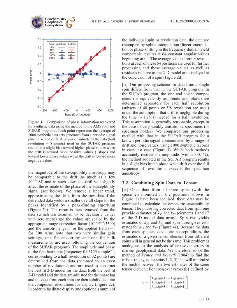
[11] Our processing scheme for data from a singlespin differs from that in the SUFAR program. Inthe SUFAR program, the sine and cosine compo-nents (or equivalently amplitude and phase) aredetermined separately for each half revolution(subsets of 40 points or 5/8 revolution are used)under the assumption that drift is negligible duringthe time (�1.25 s) needed for a half revolution.This assumption is generally reasonable, except inthe case of very weakly anisotropic specimens (orspecimen holder). We compared our processingmethod with that in the SUFAR program for aknown periodic signal contaminated by a range ofdrift and noise values, using 1000 synthetic recordsin each test case (Figure 3). While both methodsaccurately recover the amplitude (within �0.1%),the method adopted in the SUFAR program resultsin a slight bias in the phase when drift over the fullsequence of revolutions exceeds the specimenanisotropy.

3.2. Combining Spin Data to Tensor

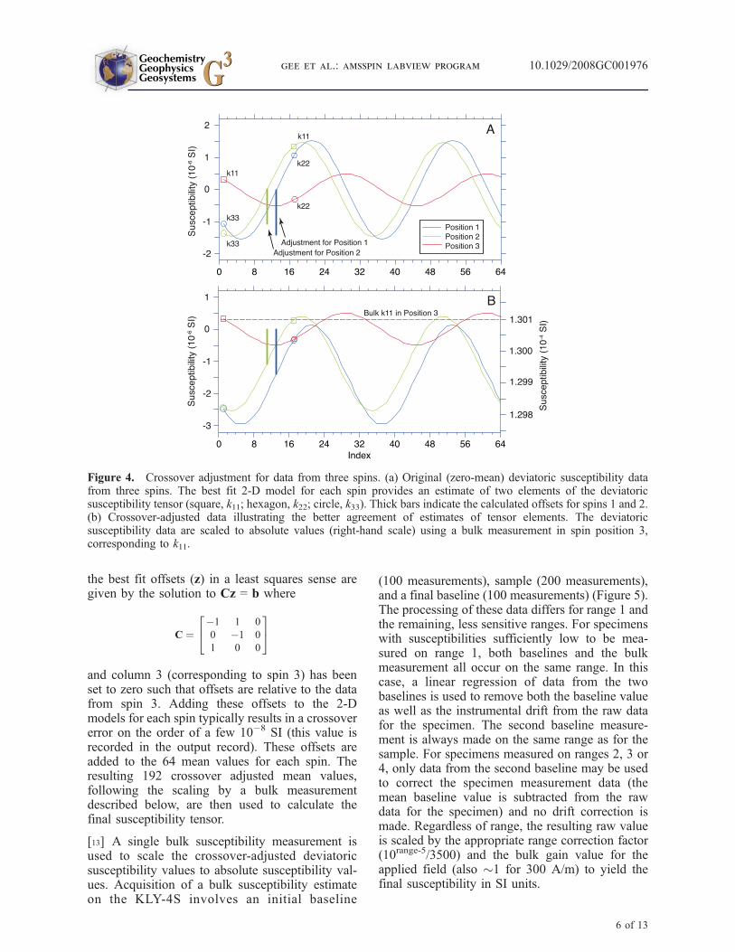
[12] Once data from all three spins (with thespecimen mounted in the positions shown inFigure 1) have been acquired, these data may becombined to calculate the deviatoric susceptibilitytensor. The phase lag corrected data from spin oneprovide estimates of k33 and k22 (elements 1 and 17of the 2-D model data array). Spin two yieldsestimates of k33 and k11 and spin three gives esti-mates for k11 and k22 (Figure 4a). Because the datafrom each spin are deviatoric susceptibilities, theestimates of a given tensor element from differentspins will in general not be the same. This problem isanalogous to the analysis of crossover errors inmarine geophysical data. We therefore adopt themethod of Prince and Forsyth [1984] to find theoffsets (z1, z2, z3 for spins 1, 2, 3) that will minimizethe misfits between the two estimates of the sametensor element. For crossover errors (b) defined by

b ¼k33 Spin1ð Þ � k33 Spin2ð Þk11 Spin2ð Þ � k11 Spin3ð Þk22 Spin3ð Þ � k22 Spin1ð Þ

24

35

Figure 3. Comparison of phase information recoveredfor synthetic data using the method in the AMSSpin andSUFAR programs. Each point represents the average of1000 synthetic data sets generated from a periodic signalplus noise and drift. Analysis of subsets of the data (halfrevolution + 8 points) used in the SUFAR programresults in a slight bias toward higher phase values whenthe drift is toward more positive values (+slope) andtoward lower phase values when the drift is toward morenegative values.



5 of 13

the best fit offsets (z) in a least squares sense aregiven by the solution to Cz = b where

C ¼�1 1 0

0 �1 0

1 0 0

24

35

and column 3 (corresponding to spin 3) has beenset to zero such that offsets are relative to the datafrom spin 3. Adding these offsets to the 2-Dmodels for each spin typically results in a crossovererror on the order of a few 10�8 SI (this value isrecorded in the output record). These offsets areadded to the 64 mean values for each spin. Theresulting 192 crossover adjusted mean values,following the scaling by a bulk measurementdescribed below, are then used to calculate thefinal susceptibility tensor.

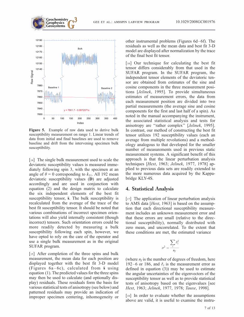
[13] A single bulk susceptibility measurement isused to scale the crossover-adjusted deviatoricsusceptibility values to absolute susceptibility val-ues. Acquisition of a bulk susceptibility estimateon the KLY-4S involves an initial baseline

(100 measurements), sample (200 measurements),and a final baseline (100 measurements) (Figure 5).The processing of these data differs for range 1 andthe remaining, less sensitive ranges. For specimenswith susceptibilities sufficiently low to be mea-sured on range 1, both baselines and the bulkmeasurement all occur on the same range. In thiscase, a linear regression of data from the twobaselines is used to remove both the baseline valueas well as the instrumental drift from the raw datafor the specimen. The second baseline measure-ment is always made on the same range as for thesample. For specimens measured on ranges 2, 3 or4, only data from the second baseline may be usedto correct the specimen measurement data (themean baseline value is subtracted from the rawdata for the specimen) and no drift correction ismade. Regardless of range, the resulting raw valueis scaled by the appropriate range correction factor(10range-5/3500) and the bulk gain value for theapplied field (also �1 for 300 A/m) to yield thefinal susceptibility in SI units.

Figure 4. Crossover adjustment for data from three spins. (a) Original (zero-mean) deviatoric susceptibility datafrom three spins. The best fit 2-D model for each spin provides an estimate of two elements of the deviatoricsusceptibility tensor (square, k11; hexagon, k22; circle, k33). Thick bars indicate the calculated offsets for spins 1 and 2.(b) Crossover-adjusted data illustrating the better agreement of estimates of tensor elements. The deviatoricsusceptibility data are scaled to absolute values (right-hand scale) using a bulk measurement in spin position 3,corresponding to k11.



6 of 13

[14] The single bulk measurement used to scale thedeviatoric susceptibility values is measured imme-diately following spin 3, with the specimen at anangle of q = 0 corresponding to k11. All 192 meandeviatoric susceptibility values (D) are adjustedaccordingly and are used in conjunction withequation (2) and the design matrix to calculatethe six independent elements of the best fitsusceptibility tensor, s. The bulk susceptibility isrecalculated from the average of the trace of thebest fit susceptibility tensor. It should be noted thatvarious combinations of incorrect specimen orien-tations will also yield internally consistent (thoughincorrect) tensors. Such orientation errors could bemore readily detected by measuring a bulksusceptibility following each spin, however, wehave opted to rely on the care of the operator anduse a single bulk measurement as in the originalSUFAR program.

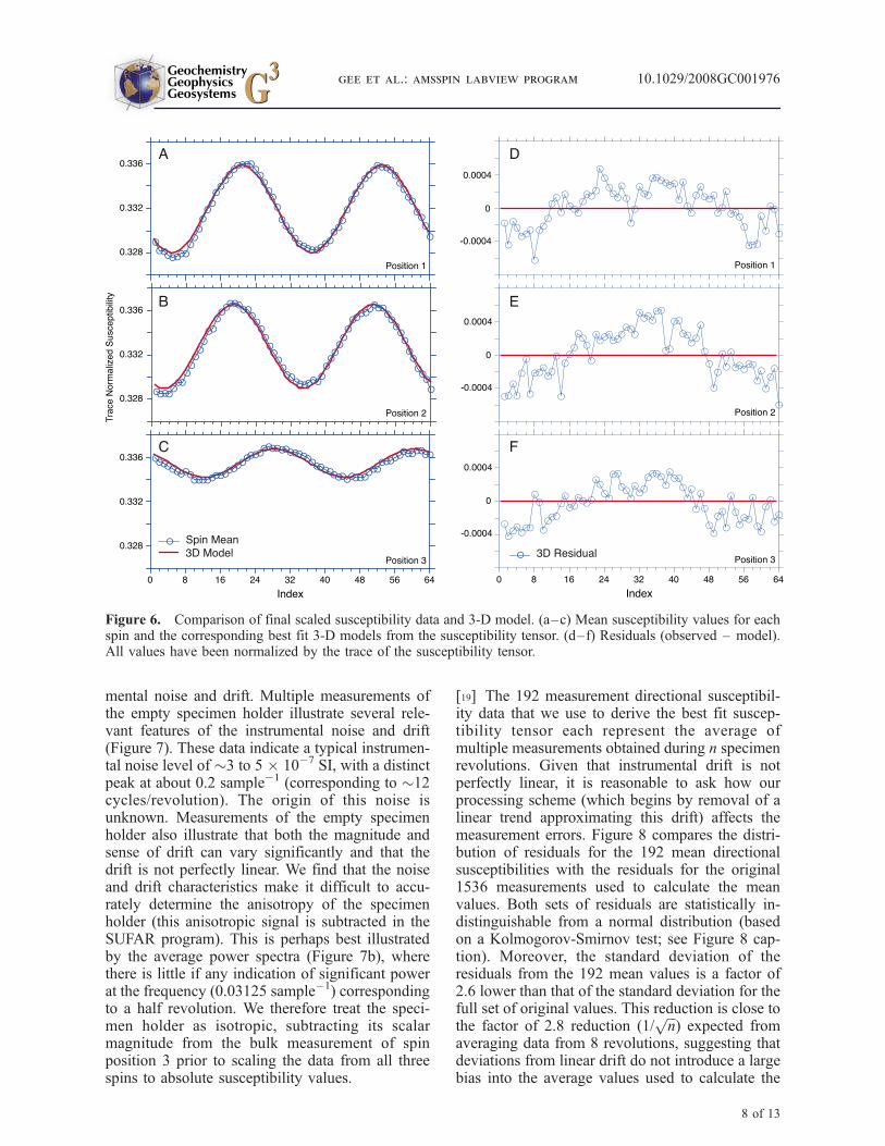
[15] After completion of the three spins and bulkmeasurement, the mean data for each position aredisplayed together with the best fit 3-D model(Figures 6a – 6c), calculated from s usingequation (1). The predicted values for the three spinsmay then be used to calculate (and optionally dis-play) residuals. These residuals form the basis forvarious statistical tests of anisotropy (see below) andpatterned residuals may provide an indication ofimproper specimen centering, inhomogeneity or

other instrumental problems (Figures 6d–6f). Theresiduals as well as the mean data and best fit 3-Dmodel are displayed after normalization by the traceof the final best fit tensor.

[16] Our technique for calculating the best fittensor differs considerably from that used in theSUFAR program. In the SUFAR program, theindependent tensor elements of the deviatoric ten-sor are obtained from estimates of the sine andcosine components in the three measurement posi-tions [Jelinek, 1995]. To provide simultaneousestimates of measurement errors, the data fromeach measurement position are divided into twopartial measurements (the average sine and cosinecomponents for the first and last half of a spin). Asnoted in the manual accompanying the instrument,the associated statistical analysis and tests foranisotropy are ‘‘rather complex’’ [Jelinek, 1995].In contrast, our method of constructing the best fittensor utilizes 192 susceptibility values (each anaverage from multiple revolutions) and a method-ology analogous to that developed for the smallernumber of measurements used in previous staticmeasurement systems. A significant benefit of thisapproach is that the linear perturbation analysistechniques [Hext, 1963; Jelinek, 1977, 1978] ap-plied to previous data sets are readily extended tothe more numerous data acquired by the Kappa-bridge KLY-4S.

4. Statistical Analysis

[17] The application of linear perturbation analysisto AMS data [Hext, 1963] is based on the assump-tion that each directional susceptibility measure-ment includes an unknown measurement error andthat these errors are small (relative to the direc-tional susceptibility), normally distributed withzero mean, and uncorrelated. To the extent thatthese conditions are met, the estimated variance

s2 ¼

Xi

d2i

nf

(where nf is the number of degrees of freedom, here192–6 or 186, and di is the measurement error asdefined in equation (3)) may be used to estimatethe angular uncertainties of the eigenvectors of thesusceptibility tensor as well as to provide statisticaltests of anisotropy based on the eigenvalues [seeHext, 1963; Jelinek, 1977, 1978; Tauxe, 1998].

[18] In order to evaluate whether the assumptionsabove are valid, it is useful to examine the instru-

Figure 5. Example of raw data used to derive bulksusceptibility measurement on range 1. Linear trends ofdata from initial and final baselines are used to removebaseline and drift from the intervening specimen bulksusceptibility.



7 of 13

mental noise and drift. Multiple measurements ofthe empty specimen holder illustrate several rele-vant features of the instrumental noise and drift(Figure 7). These data indicate a typical instrumen-tal noise level of �3 to 5 � 10�7 SI, with a distinctpeak at about 0.2 sample�1 (corresponding to �12cycles/revolution). The origin of this noise isunknown. Measurements of the empty specimenholder also illustrate that both the magnitude andsense of drift can vary significantly and that thedrift is not perfectly linear. We find that the noiseand drift characteristics make it difficult to accu-rately determine the anisotropy of the specimenholder (this anisotropic signal is subtracted in theSUFAR program). This is perhaps best illustratedby the average power spectra (Figure 7b), wherethere is little if any indication of significant powerat the frequency (0.03125 sample�1) correspondingto a half revolution. We therefore treat the speci-men holder as isotropic, subtracting its scalarmagnitude from the bulk measurement of spinposition 3 prior to scaling the data from all threespins to absolute susceptibility values.

[19] The 192 measurement directional susceptibil-ity data that we use to derive the best fit suscep-tibility tensor each represent the average ofmultiple measurements obtained during n specimenrevolutions. Given that instrumental drift is notperfectly linear, it is reasonable to ask how ourprocessing scheme (which begins by removal of alinear trend approximating this drift) affects themeasurement errors. Figure 8 compares the distri-bution of residuals for the 192 mean directionalsusceptibilities with the residuals for the original1536 measurements used to calculate the meanvalues. Both sets of residuals are statistically in-distinguishable from a normal distribution (basedon a Kolmogorov-Smirnov test; see Figure 8 cap-tion). Moreover, the standard deviation of theresiduals from the 192 mean values is a factor of2.6 lower than that of the standard deviation for thefull set of original values. This reduction is close tothe factor of 2.8 reduction (1/

ffiffiffin

p) expected from

averaging data from 8 revolutions, suggesting thatdeviations from linear drift do not introduce a largebias into the average values used to calculate the

Figure 6. Comparison of final scaled susceptibility data and 3-D model. (a–c) Mean susceptibility values for eachspin and the corresponding best fit 3-D models from the susceptibility tensor. (d–f) Residuals (observed – model).All values have been normalized by the trace of the susceptibility tensor.



8 of 13

Figure 7. Instrumental drift and noise for the Kappabridge KLY-4S. (a) Representative data from spins(8 revolutions; boundaries denoted by dotted vertical lines) of empty specimen holder (i.e., ring with 64 notches only,without cube). (b) Average multitaper power spectral density (1 s errors in red) based on detrended data from 30 spinswith empty specimen holder, including the data shown in Figure 7a. Note the lack of a distinct peak at 0.03125sample�1, corresponding to a half revolution. The frequency resolution of the multitaper estimate is shown by theblue vertical band.

Figure 8. Distribution of residuals for a representative specimen. (a) Quantile-quantile plot for all data acquired andfor the 192 averaged values (inset). Both distributions are statistically indistinguishable from a normal distributionbased on Kolmogorov-Smirnov (K-S) test (D, K-S statistic; Dc, critical value). (b) Histograms of residuals for all dataacquired (blue) and for the 192 averaged values (red) used in calculating the final susceptibility tensor.



9 of 13

susceptibility tensor. The RMS magnitude of the192 mean residuals is small (8 � 10�8 SI relativeto the bulk susceptibility of 1.3 � 10�4 SI for thespecimen in Figure 8) and these residuals arenormally distributed with zero mean. While theresiduals may not be independent in all cases(particularly when the sample is poorly centeredor inhomogeneous), it appears that the assumptionsof the linear perturbation analysis are generallysatisfied.

[20] The formulations developed for estimating theuncertainties on the eigenvectors of the suscepti-bility tensor and the statistical tests for anisotropy[Hext, 1963] can be applied with minor modifica-tions for the number of degrees of freedom. Spe-cifically, the semi-angles of the confidence ellipsesfor the eigenvectors are given by

e21 ¼ e12 ¼ tan�1 f s=2 t1 � t2ð Þ½ �

e32 ¼ e23 ¼ tan�1 f s=2 t2 � t3ð Þ½ �

e31 ¼ e13 ¼ tan�1 f s=2 t1 � t3ð Þ½ �

where t1 t2 t3 are the eigenvalues and

f ¼ffiffiffiffiffiffiffiffiffiffiffiffiffiffiffiffiffiffiffiffiffiffiffiffiffiffiffiffiffiffiffiffiffiffiffiffiffiffi2 F

2;nfð Þ; 1� pð Þ� �r

¼ffiffiffiffiffiffiffiffiffiffiffiffiffiffiffiffiffiffiffiffiffiffiffiffiffiffiffiffiffiffiffiffiffiffiffiffiffiffiffiffiffiffiffi2 F 2;186ð Þ; 1� 0:05ð Þ� �q

¼ffiffiffiffiffiffiffiffiffiffiffiffiffiffiffi2 3:04ð Þ

p¼ 2:465

for nf = 192 � 6 or 186 degrees of freedom at the95% confidence level. The corresponding F tests

for anisotropy remain the same as for susceptibilitytensors based on a smaller number of measurementpositions:

F ¼ 0:4 t21 þ t22 þ t23 � 3c2b

� �=s2

F12 ¼ 0:5 t1 � t2ð Þ=s½ �2F23 ¼ 0:5 t2 � t3ð Þ=s½ �2

where the bulk susceptibility (cb) is given by cb =(s1 + s2 + s3)/3. The critical values (at the 95%confidence level) for the F tests also remain thesame. The susceptibility tensor is statisticallyisotropic if F < 3.4817 and is statistically oblate ifF12 < 4.2565 or statistically prolate if F23 < 4.2565.

[21] It should be noted that uncertainty estimatesfor the eigenvectors that are displayed at thecompletion of a measurement in the AMSSpinprogram differ from those in the SUFAR program.The former are based on linear perturbation anal-ysis [Hext, 1963; Jelinek, 1977, 1978] in whicherror angles are defined along the principal planesof the susceptibility ellipsoid whereas in theSUFAR program these error angles are oblique,reflecting the interplay between the orientations ofprincipal planes and measuring planes. Neverthe-less, the numerical values provided by the theseapproaches are similar, characterizing the uncer-tainties in determination of the principal directionsin a very similar way.

5. Comparison of Results With SUFARProgram

[22] The treatment of directional susceptibility datain the AMSSpin program differs from that in theSUFAR program and so it is not surprising that thecalculated tensors differ somewhat. In order tocompare the results from our new program andthe SUFAR program, we first measured a suite of33 specimens with a range of anisotropy values(ratio of max/min eigenvalues = 1.02–1.55) withboth programs. Bulk susceptibilities from the twoprograms agree well (mean difference = 0.3%).The root mean square (rms) deviation of the sixindependent elements (normalized by the trace) ofthe susceptibility tensors from these two measure-ments differ by an average of 0.0009. Althoughthis discrepancy is large relative to the standarderror, differences in the two measurements alsoinclude uncertainties in positioning the specimen inthe specimen holder.

[23] A more direct test is to compare the tensorsobtained by processing the same raw data by both

Figure 9. Comparison of susceptibility tensors derivedby processing the same raw data using the AMSSpinprogram and algorithm in SUFAR program.



10 of 13

the method developed for the AMSSpin programand the processing algorithm of the SUFAR pro-gram. The RMS deviations of the susceptibilitytensors derived by these two processing techniquesaverages �0.0002, with slightly larger RMS devi-ations for specimens with higher degrees of anisot-ropy (Figure 9). For all but two of these 33specimens the RMS deviation is less than thestandard error (s) calculated from the AMSSpinprogram (this error estimate is on average 3.5 timesthat of the SUFAR program). Comparison ofmultiple measurements of these same samples(measured on different days) using the AMSSpinprogram suggests that specimen orientation errorsare comparable to the standard error (rms devia-tions average 0.0003). On the basis of these com-parisons, we suggest that differences between theprocessing methods in the AMSSpin and SUFARprograms are smaller than or comparable to uncer-tainties associated with specimen positioning.

6. Conclusions

[24] We have developed a graphical program thatallows the acquisition of AMS data from theKappabridge KLY-4S. This program provides realtime display of susceptibility data acquired duringa spin and the display of best fit 2-D and 3-Dmodels to the data (and the resulting residuals). Inaddition, the program allows the display of all

previously measured data from a specimen (sam-ple, site, or study) together with the current spec-imen results to allow evaluation of within siteconsistency. The treatment of the sample holderas isotropic, processing of the data from an indi-vidual spin, as well as the method of combining thethree spins to yield the final susceptibility tensor,differ significantly from the methods used in theSUFAR program. Despite the different processingmethods the AMSSpin and SUFAR programs yieldresults that are quite similar, with deviations thatare comparable to or smaller than uncertaintiesintroduced by sample positioning. We find thatby utilizing mean directional susceptibility valuesfor 192 positions that the measurement errors aresuitable for linear perturbation analysis, providinga well established means of statistically character-izing the AMS data acquired with the KappabridgeKLY-4S.

[25] An executable version of the LabVIEW pro-gram, together with additional documentation, isavailable from the EarthRef.org Digital Archive(ERDA) at http://earthref.org. Although the pro-gram is presently available only for a Macintosh,the source code is platform independent and will beported to other platforms in the future. Modifica-tions that will allow use of the program with aKLY-3S are also underway. Output from this pro-gram can be converted to the MAGIC standardformat for plotting with the PmagPy software thatis also available at this same site (see Appendix Afor example output).

Appendix A

[26] To validate the new AMSSpin program, wehave also compared the results from this program(and the Kappabridge KLY-4S) with resultsobtained from a Kappabridge KLY-2 static mea-surement system. AMS measurements were madeon both instruments for approximately 100 sam-ples, with bulk susceptibilities ranging from 4 �10�5 to 7 � 10�2 SI. Bulk susceptibilities with thetwo instruments typically agree within 0.5%, withmaximum deviations of approximately 3%. TheKappabridge KLY-4S and AMSSpin program yieldbetter defined susceptibility tensors (as measuredby the standard error, sigma). On average sigmavalues are a factor of 2–3 smaller than thosedetermined with the Kappabridge KLY-2, asexpected from the larger number of measurementsusing the KLY-4S, though the improvement is lesspronounced in samples with lower bulk suscepti-bilities (Figure A1). The value of sigma also varies

Figure A1. Comparison of measurement errors (asquantified by the trace normalized value of sigma) forthe Kappabridge KLY-4S and KLY-2. Inset shows ahistogram of the ratio of uncertainties (KLY-4S/KLY-2).



11 of 13

both as a function of applied field and measure-ment range, with higher values at lower appliedfields and when susceptibilities are at the lower endof a measurement range. Differences in the sus-ceptibility tensors from the two instruments arealso a function of bulk susceptibility. For speci-mens with susceptibilities of �10�4 SI, the rootmean square difference in the six independentsusceptibility tensor elements (normalized by thetrace) is approximately 0.001 and this deviationdecreases to about 0.0001 for a bulk susceptibilityof �10�1 SI.

[27] The standard output of the AMSSpin programincludes a minimal amount of information: thespecimen name, the six independent elements ofthe susceptibility tensor (trace normalized, in spec-imen coordinates) and sigma, the bulk susceptibil-ity and a small number of parameters (e.g., volume,applied field) relevant to the measurement. Soft-ware available with the PmagPy distribution allowsconversion of the data from AMSSpin to thestandard MAGIC format. Data can be analyzed ina variety of ways (e.g., generating error ellipses fora site using either bootstrap resampling or Hextstatistics) and plotted in a variety of coordinatesystems (see Figure A2 for sample output).

[28] While the errors associated with measure-ments on the Kappabridge KLY-4S are typicallysmall and normally distributed for most specimens,we have found that this is not the case for somesamples. Figure A3 illustrates results from a basal-tic dike with a high bulk susceptibility (6.3 �10�2 SI) and a very low degree of anisotropy. In

Figure A2. Example output from processing software of the PmagPy software distribution. (a) Equal area plot ofeigenvectors for specimens from a single sampling site. Circles, triangles, and squares represent the eigenvectorsassociated with the minimum, intermediate, and maximum eigenvalues, respectively. (b) Nonparametric bootstrappseudosamples generated from the specimen data shown in Figure A2a. (c) Cumulative distribution functions for theeigenvalues of bootstrap pseudosamples. Vertical lines indicate the 95% confidence bounds of the site meaneigenvalues.

Figure A3. Example of specimen with directionalsusceptibility variations deviating significantly from thatexpected from a symmetric second-order tensor. Devia-toric susceptibility data for each revolution are shown inblue and the best fit 2-D model is shown in red for eachof the three spins. Note that each plot has a differentvertical scale.



12 of 13

this case, the directional susceptibility signal forspins 1 and 2 deviates substantially from thatexpected from a symmetric second-order tensor.Such deviations may arise from inhomogeneitywithin the specimen (or possibly from other artifactsof the measurement system such as the specimenbeing offset from the center of the coil). By display-ing the measured and best fit 2-D and 3-D models tothe data, the AMSSpin program provides the userwith a means of identifying such data as problem-atic.

[29] The confidence intervals for the principalsusceptibility values are affected by the orientationof the measurements relative to the anisotropicsusceptibility of the specimen [Hext, 1963; Owens,2000]. This effect can be minimized by the use of ameasurement scheme that is rotatable [Hext, 1963],i.e., one in which the measurements are evenlyspaced over the unit sphere such that error varian-ces do not depend on the relative orientation of thespecimen and measurement positions. The direc-tional susceptibility data acquired at evenly spacedintervals during each spin constitute such a rotat-able design for determining the susceptibility ten-sor in each plane. The distribution of measurementpositions on three orthogonal planes, however,inevitably introduces a small degree of nonrotat-ability in the measurement design. Although theprocessing differs in the AMSSpin program andthe SUFAR program, both approaches utilize thesame directional measurements and therefore areaffected by this nonrotatability. We note that theaddition of spins about two diagonal rotation axesin the specimen coordinate system could be intro-duced to further improve the rotatability.

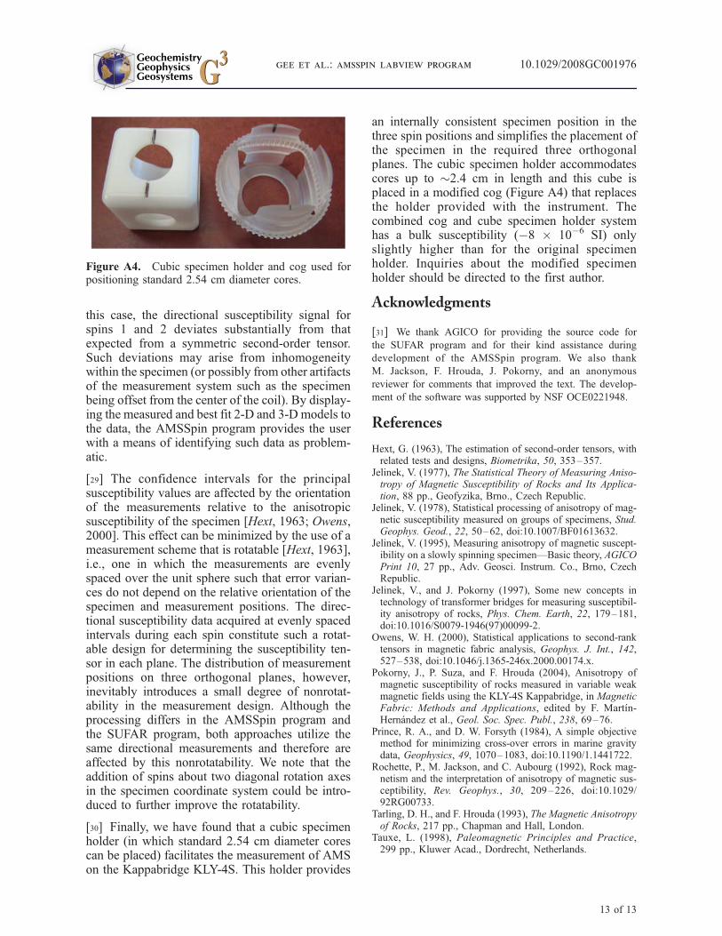
[30] Finally, we have found that a cubic specimenholder (in which standard 2.54 cm diameter corescan be placed) facilitates the measurement of AMSon the Kappabridge KLY-4S. This holder provides

an internally consistent specimen position in thethree spin positions and simplifies the placement ofthe specimen in the required three orthogonalplanes. The cubic specimen holder accommodatescores up to �2.4 cm in length and this cube isplaced in a modified cog (Figure A4) that replacesthe holder provided with the instrument. Thecombined cog and cube specimen holder systemhas a bulk susceptibility (�8 � 10�6 SI) onlyslightly higher than for the original specimenholder. Inquiries about the modified specimenholder should be directed to the first author.

Acknowledgments

[31] We thank AGICO for providing the source code for

the SUFAR program and for their kind assistance during

development of the AMSSpin program. We also thank

M. Jackson, F. Hrouda, J. Pokorny, and an anonymous

reviewer for comments that improved the text. The develop-

ment of the software was supported by NSF OCE0221948.

References

Hext, G. (1963), The estimation of second-order tensors, withrelated tests and designs, Biometrika, 50, 353–357.

Jelinek, V. (1977), The Statistical Theory of Measuring Aniso-tropy of Magnetic Susceptibility of Rocks and Its Applica-tion, 88 pp., Geofyzika, Brno., Czech Republic.

Jelinek, V. (1978), Statistical processing of anisotropy of mag-netic susceptibility measured on groups of specimens, Stud.Geophys. Geod., 22, 50–62, doi:10.1007/BF01613632.

Jelinek, V. (1995), Measuring anisotropy of magnetic suscept-ibility on a slowly spinning specimen—Basic theory, AGICOPrint 10, 27 pp., Adv. Geosci. Instrum. Co., Brno, CzechRepublic.

Jelinek, V., and J. Pokorny (1997), Some new concepts intechnology of transformer bridges for measuring susceptibil-ity anisotropy of rocks, Phys. Chem. Earth, 22, 179–181,doi:10.1016/S0079-1946(97)00099-2.

Owens, W. H. (2000), Statistical applications to second-ranktensors in magnetic fabric analysis, Geophys. J. Int., 142,527–538, doi:10.1046/j.1365-246x.2000.00174.x.

Pokorny, J., P. Suza, and F. Hrouda (2004), Anisotropy ofmagnetic susceptibility of rocks measured in variable weakmagnetic fields using the KLY-4S Kappabridge, in MagneticFabric: Methods and Applications, edited by F. Martın-Hernandez et al., Geol. Soc. Spec. Publ., 238, 69–76.

Prince, R. A., and D. W. Forsyth (1984), A simple objectivemethod for minimizing cross-over errors in marine gravitydata, Geophysics, 49, 1070–1083, doi:10.1190/1.1441722.

Rochette, P., M. Jackson, and C. Aubourg (1992), Rock mag-netism and the interpretation of anisotropy of magnetic sus-ceptibility, Rev. Geophys., 30, 209–226, doi:10.1029/92RG00733.

Tarling, D. H., and F. Hrouda (1993), The Magnetic Anisotropyof Rocks, 217 pp., Chapman and Hall, London.

Tauxe, L. (1998), Paleomagnetic Principles and Practice,299 pp., Kluwer Acad., Dordrecht, Netherlands.

Figure A4. Cubic specimen holder and cog used forpositioning standard 2.54 cm diameter cores.



13 of 13

AMSSpin: A LabVIEW program for measuring the anisotropy of magnetic susceptibility with the Kappabridge KLY-4S

Documents