Welcome message from author
This document is posted to help you gain knowledge. Please leave a comment to let me know what you think about it! Share it to your friends and learn new things together.
Transcript


Amira 5Amira User’s Guide

Intended UseAmira R© is intended for research use only. It is not a medical device.Copyright Informationc©1995-2009 Konrad-Zuse-Zentrum fur Informationstechnik Berlin (ZIB), Germanyc©1999-2009 Visage Imaging
All rights reserved.
Trademark Information:Amira is being jointly developed by Konrad-Zuse-Zentrum fur Informationstechnik Berlin (ZIB) andVisage Imaging.Amira R© is a registered trademark of Konrad-Zuse-Zentrum fur Informationstechnik Berlin and VisageImaging.HardCopy, MeshViz, VolumeViz, TerrainViz, ScaleViz are trademarks of Mercury Computer SystemsS.A.S.Mercury Computer Systems S.A.S. is a source licensee of OpenGL R©, Open Inventor R© from SiliconGraphics, Inc.OpenGL R© and Open Inventor R© are registered trademarks of Silicon Graphics, Inc.All other products and company names are trademarks or registered trademarks of their respectivecompanies.This manual has been prepared for Visage Imaging licensees solely for use in connection with softwaresupplied by Visage Imaging and is furnished under a written license agreement. This material may notbe used, reproduced or disclosed, in whole or in part, except as permitted in the license agreement orby prior written authorization of Visage Imaging. Users are cautioned that Visage Imaging reserves theright to make changes without notice to the specifications and materials contained herein and shall notbe responsible for any damages (including consequential) caused by reliance on the materials presented,including but not limited to typographical, arithmetic or listing errors.
Contents
I Amira User’s Guide 1
1 Introduction 31.1 Overview . . . . . . . . . . . . . . . . . . . . . . . . . . . . . . 41.2 Features overview . . . . . . . . . . . . . . . . . . . . . . . . . . 4
1.2.1 Data import . . . . . . . . . . . . . . . . . . . . . . . . . 51.2.2 Viewing, navigation, interactivity . . . . . . . . . . . . . 61.2.3 Visualization of 3D Image Data . . . . . . . . . . . . . . 61.2.4 Image processing . . . . . . . . . . . . . . . . . . . . . . 71.2.5 Model reconstruction . . . . . . . . . . . . . . . . . . . . 81.2.6 Visualization of 3D models and numerical data . . . . . . 91.2.7 General Data Processing and Data Analysis . . . . . . . . 101.2.8 Matlab integration . . . . . . . . . . . . . . . . . . . . . 121.2.9 High Performance Visualization . . . . . . . . . . . . . . 121.2.10 Automation, Customization, Extensibility . . . . . . . . . 12
1.3 Application Areas . . . . . . . . . . . . . . . . . . . . . . . . . . 121.4 Options . . . . . . . . . . . . . . . . . . . . . . . . . . . . . . . 13
2 First steps in Amira 172.1 Getting Started . . . . . . . . . . . . . . . . . . . . . . . . . . . 18
2.1.1 Loading Data . . . . . . . . . . . . . . . . . . . . . . . . 192.1.2 Invoking Editors . . . . . . . . . . . . . . . . . . . . . . 212.1.3 Visualizing Data . . . . . . . . . . . . . . . . . . . . . . 222.1.4 Interaction with the Viewer . . . . . . . . . . . . . . . . . 23
2.2 How to load image data . . . . . . . . . . . . . . . . . . . . . . . 262.2.1 The Amira File Browser . . . . . . . . . . . . . . . . . . 262.2.2 Reading 3D Image Data from Multiple 2D Slices . . . . . 272.2.3 Setting the Bounding Box . . . . . . . . . . . . . . . . . 282.2.4 The Stacked Slices file format . . . . . . . . . . . . . . . 29
i
Contents
2.2.5 Working with Large Disk Data . . . . . . . . . . . . . . . 302.3 Visualizing 3D Images . . . . . . . . . . . . . . . . . . . . . . . 32
2.3.1 Orthogonal Slices . . . . . . . . . . . . . . . . . . . . . . 332.3.2 Simple Data Analysis . . . . . . . . . . . . . . . . . . . . 332.3.3 Resampling the Data . . . . . . . . . . . . . . . . . . . . 342.3.4 Displaying an Isosurface . . . . . . . . . . . . . . . . . . 362.3.5 Cropping the Data . . . . . . . . . . . . . . . . . . . . . 362.3.6 Volume Rendering . . . . . . . . . . . . . . . . . . . . . 37
2.4 Segmentation of 3D Images . . . . . . . . . . . . . . . . . . . . . 402.4.1 Interactive Image Segmentation . . . . . . . . . . . . . . 402.4.2 Volume Measurement . . . . . . . . . . . . . . . . . . . 422.4.3 Threshold Segmentation . . . . . . . . . . . . . . . . . . 432.4.4 Refining Threshold Segmentation Results . . . . . . . . . 43
2.5 Surface Reconstruction from 3D Images . . . . . . . . . . . . . . 452.5.1 Extracting Surfaces from Segmentation Results . . . . . . 452.5.2 Simplifying the Surface . . . . . . . . . . . . . . . . . . 45
2.6 Creating a Tetrahedral Grid from a Triangular Surface . . . . . . . 472.6.1 Simplifying the Surface . . . . . . . . . . . . . . . . . . 472.6.2 Editing the Surface . . . . . . . . . . . . . . . . . . . . . 492.6.3 Generation of a Tetrahedral Grid . . . . . . . . . . . . . . 51
2.7 Warping and Registration Using Landmarks . . . . . . . . . . . . 532.7.1 Displaying Data Sets in Two Viewers . . . . . . . . . . . 542.7.2 Creating a Landmark Set . . . . . . . . . . . . . . . . . . 542.7.3 Registration via a Rigid Transformation . . . . . . . . . . 572.7.4 Warping Two Image Volumes . . . . . . . . . . . . . . . 57
2.8 Registration of 3D image data sets . . . . . . . . . . . . . . . . . 582.8.1 Basic Manual Registration . . . . . . . . . . . . . . . . . 592.8.2 Automatic Registration . . . . . . . . . . . . . . . . . . . 602.8.3 Image Fusion . . . . . . . . . . . . . . . . . . . . . . . . 61
2.9 Alignment of 2D Physical Cross-sections . . . . . . . . . . . . . 622.9.1 Basic Manual Alignment . . . . . . . . . . . . . . . . . . 632.9.2 Alignment Via Landmarks . . . . . . . . . . . . . . . . . 652.9.3 Optimizing the Quality Function . . . . . . . . . . . . . . 672.9.4 Resampling the Input Data . . . . . . . . . . . . . . . . . 672.9.5 Using a Reference Image . . . . . . . . . . . . . . . . . . 68
2.10 Visualization of Vector Fields . . . . . . . . . . . . . . . . . . . . 692.10.1 Simple Vector Representation . . . . . . . . . . . . . . . 692.10.2 Illuminated Stream Lines . . . . . . . . . . . . . . . . . . 71
ii
Contents
2.10.3 Animated Particle Plot . . . . . . . . . . . . . . . . . . . 722.11 Creating animated demonstrations . . . . . . . . . . . . . . . . . 73
2.11.1 Creating a Network . . . . . . . . . . . . . . . . . . . . . 742.11.2 Animating an OrthoSlice Module . . . . . . . . . . . . . 742.11.3 Activating a Module in the Viewer Window . . . . . . . . 772.11.4 Using a Camera Rotation . . . . . . . . . . . . . . . . . . 782.11.5 Editing or Removing an Already Defined Event . . . . . . 792.11.6 Overlaying the Bone with Skin . . . . . . . . . . . . . . . 792.11.7 Using Clipping to Add the Skin Gradually . . . . . . . . . 802.11.8 More Comments on Clipping . . . . . . . . . . . . . . . 832.11.9 Breaks and Function Keys . . . . . . . . . . . . . . . . . 842.11.10 Loops and Go-to . . . . . . . . . . . . . . . . . . . . . . 852.11.11 Storing and Replaying the Animation Sequence . . . . . . 86
2.12 Creating movie files . . . . . . . . . . . . . . . . . . . . . . . . . 862.12.1 Attaching MovieMaker to a Camera Path . . . . . . . . . 872.12.2 Attaching MovieMaker to DemoMaker . . . . . . . . . . 89
2.13 Using MATLAB Scripts . . . . . . . . . . . . . . . . . . . . . . 902.13.1 Lowpass Filtering on Images . . . . . . . . . . . . . . . . 902.13.2 Thresholding on a Volume . . . . . . . . . . . . . . . . . 93
2.14 Introduction to the Filament Editor . . . . . . . . . . . . . . . . . 932.14.1 Exploration of the volume data . . . . . . . . . . . . . . . 942.14.2 Automatic extraction of the dendritic tree . . . . . . . . . 942.14.3 Filament Tracing . . . . . . . . . . . . . . . . . . . . . . 972.14.4 Visualize the network . . . . . . . . . . . . . . . . . . . . 982.14.5 Alternative way to extract a network using the Segmenta-
tion Editor . . . . . . . . . . . . . . . . . . . . . . . . . 992.15 Introduction to the Multi-planar Viewer . . . . . . . . . . . . . . 100
2.15.1 Exploration of the volume data . . . . . . . . . . . . . . . 1012.15.2 Explore two data sets using fusion mode . . . . . . . . . . 1022.15.3 Manually register two data sets . . . . . . . . . . . . . . . 104
3 Program Description 1073.1 Interface Components . . . . . . . . . . . . . . . . . . . . . . . . 107
3.1.1 File Menu . . . . . . . . . . . . . . . . . . . . . . . . . . 1073.1.2 Edit Menu . . . . . . . . . . . . . . . . . . . . . . . . . 1103.1.3 Pool Menu . . . . . . . . . . . . . . . . . . . . . . . . . 1123.1.4 Explorer Menu . . . . . . . . . . . . . . . . . . . . . . . 1143.1.5 Create Menu . . . . . . . . . . . . . . . . . . . . . . . . 114
iii
Contents
3.1.6 View Menu . . . . . . . . . . . . . . . . . . . . . . . . . 1153.1.7 Online Help . . . . . . . . . . . . . . . . . . . . . . . . . 1183.1.8 Main Window . . . . . . . . . . . . . . . . . . . . . . . . 1213.1.9 Viewer Window . . . . . . . . . . . . . . . . . . . . . . . 1313.1.10 Console Window . . . . . . . . . . . . . . . . . . . . . . 1363.1.11 File Dialog . . . . . . . . . . . . . . . . . . . . . . . . . 1373.1.12 Job Dialog . . . . . . . . . . . . . . . . . . . . . . . . . 1393.1.13 Preferences Dialog . . . . . . . . . . . . . . . . . . . . . 1413.1.14 Snapshot Dialog . . . . . . . . . . . . . . . . . . . . . . 1463.1.15 System Information Dialog . . . . . . . . . . . . . . . . . 147
3.2 General Concepts . . . . . . . . . . . . . . . . . . . . . . . . . . 1483.2.1 Class Structure . . . . . . . . . . . . . . . . . . . . . . . 1483.2.2 Scalar Field and Vector Fields . . . . . . . . . . . . . . . 1503.2.3 Coordinates and Grids . . . . . . . . . . . . . . . . . . . 1513.2.4 Surface Data . . . . . . . . . . . . . . . . . . . . . . . . 1523.2.5 Vertex Set . . . . . . . . . . . . . . . . . . . . . . . . . . 1533.2.6 Transformations . . . . . . . . . . . . . . . . . . . . . . 1533.2.7 Parameters . . . . . . . . . . . . . . . . . . . . . . . . . 1543.2.8 Shadowing . . . . . . . . . . . . . . . . . . . . . . . . . 1543.2.9 Sub-application Concept . . . . . . . . . . . . . . . . . . 155
4 Technical Information 1574.1 Data Import . . . . . . . . . . . . . . . . . . . . . . . . . . . . . 1574.2 Command Line Options . . . . . . . . . . . . . . . . . . . . . . . 1584.3 Environment Variables . . . . . . . . . . . . . . . . . . . . . . . 1594.4 User-defined start-up script . . . . . . . . . . . . . . . . . . . . . 1614.5 System Requirements . . . . . . . . . . . . . . . . . . . . . . . . 162
4.5.1 Troubleshooting . . . . . . . . . . . . . . . . . . . . . . 1634.5.2 Microsoft Windows . . . . . . . . . . . . . . . . . . . . . 1644.5.3 Linux . . . . . . . . . . . . . . . . . . . . . . . . . . . . 1644.5.4 Mac OS . . . . . . . . . . . . . . . . . . . . . . . . . . . 165
4.6 Amira License Manager . . . . . . . . . . . . . . . . . . . . . . . 1664.6.1 Contents . . . . . . . . . . . . . . . . . . . . . . . . . . 1664.6.2 About Password Protection . . . . . . . . . . . . . . . . . 1664.6.3 About the Amira License Manager . . . . . . . . . . . . . 1664.6.4 Troubleshooting . . . . . . . . . . . . . . . . . . . . . . 1674.6.5 Using TGS LICENSE DEBUG . . . . . . . . . . . . . . 1684.6.6 Contacting the License Administrator . . . . . . . . . . . 170
iv
Contents
4.6.7 Contacting Technical Support . . . . . . . . . . . . . . . 1704.7 Notes for Mac users . . . . . . . . . . . . . . . . . . . . . . . . . 1714.8 Amira and the /3GB switch . . . . . . . . . . . . . . . . . . . . . 171
4.8.1 The Problem . . . . . . . . . . . . . . . . . . . . . . . . 1724.8.2 How to activate the /3GB switch . . . . . . . . . . . . . . 172
5 Scripting 1755.1 Introduction . . . . . . . . . . . . . . . . . . . . . . . . . . . . . 1755.2 Introduction to Tcl . . . . . . . . . . . . . . . . . . . . . . . . . 176
5.2.1 Tcl Lists, Commands, Comments . . . . . . . . . . . . . 1765.2.2 Tcl Variables . . . . . . . . . . . . . . . . . . . . . . . . 1775.2.3 Tcl Command Substitution . . . . . . . . . . . . . . . . . 1785.2.4 Tcl Control Structures . . . . . . . . . . . . . . . . . . . 1785.2.5 User-Defined Tcl Procedures . . . . . . . . . . . . . . . . 1805.2.6 List and String Manipulation . . . . . . . . . . . . . . . . 181
5.3 Amira Script Interface . . . . . . . . . . . . . . . . . . . . . . . . 1825.3.1 Predefined Variables . . . . . . . . . . . . . . . . . . . . 1845.3.2 Object commands . . . . . . . . . . . . . . . . . . . . . . 1855.3.3 Global Commands . . . . . . . . . . . . . . . . . . . . . 185
5.4 Amira Script File . . . . . . . . . . . . . . . . . . . . . . . . . . 1995.5 Configuring Popup Menus . . . . . . . . . . . . . . . . . . . . . 2005.6 Registering pick callbacks . . . . . . . . . . . . . . . . . . . . . 203
6 Demo Framework 2076.1 Directory Structure and Files . . . . . . . . . . . . . . . . . . . . 207
6.1.1 Directories and Files in src/ . . . . . . . . . . . . . . . . 2086.1.2 Data Storage . . . . . . . . . . . . . . . . . . . . . . . . 214
6.2 Selecting Demos . . . . . . . . . . . . . . . . . . . . . . . . . . 2156.3 Prerequisites . . . . . . . . . . . . . . . . . . . . . . . . . . . . . 218
II Molecular Option User’s Guide 219
7 Molecular Option Introduction 2217.1 First Steps with Molecular Visualization in Amira . . . . . . . . . 221
7.1.1 Getting Started with Molecular Visualization . . . . . . . 2227.1.2 Selection, Labeling, and Masking . . . . . . . . . . . . . 2257.1.3 Alignment of Molecules . . . . . . . . . . . . . . . . . . 232
v
Contents
7.1.4 Molecular Surfaces . . . . . . . . . . . . . . . . . . . . . 2377.1.5 Sequential and Structural Alignment . . . . . . . . . . . . 2407.1.6 Editing of molecules . . . . . . . . . . . . . . . . . . . . 2427.1.7 Molecular Interfaces . . . . . . . . . . . . . . . . . . . . 2457.1.8 Measurement . . . . . . . . . . . . . . . . . . . . . . . . 248
7.2 Molecular Data Structures . . . . . . . . . . . . . . . . . . . . . 2497.2.1 Internal Structure of Molecules . . . . . . . . . . . . . . 249
7.3 Displaying Molecules . . . . . . . . . . . . . . . . . . . . . . . . 2497.3.1 Coloring Molecules . . . . . . . . . . . . . . . . . . . . . 2507.3.2 Selecting and Filtering atoms . . . . . . . . . . . . . . . 252
7.4 Aligning Molecules . . . . . . . . . . . . . . . . . . . . . . . . . 2547.4.1 Alignment of Trajectories . . . . . . . . . . . . . . . . . 2547.4.2 Mean Distance Alignment . . . . . . . . . . . . . . . . . 2567.4.3 Sequence alignment . . . . . . . . . . . . . . . . . . . . 256
7.5 Visualizing Molecular Trajectories and Metastable Conformations 2577.6 Atom Expressions . . . . . . . . . . . . . . . . . . . . . . . . . . 257
7.6.1 Overview . . . . . . . . . . . . . . . . . . . . . . . . . . 2577.6.2 Grammar . . . . . . . . . . . . . . . . . . . . . . . . . . 2587.6.3 Literals . . . . . . . . . . . . . . . . . . . . . . . . . . . 2587.6.4 Operators . . . . . . . . . . . . . . . . . . . . . . . . . . 2597.6.5 Shortcuts . . . . . . . . . . . . . . . . . . . . . . . . . . 2617.6.6 Further Examples . . . . . . . . . . . . . . . . . . . . . . 261
III Virtual Reality Option User’s Guide 263
8 Virtual Reality Option User’s Guide 2658.1 Virtual Reality Option Essentials . . . . . . . . . . . . . . . . . . 266
8.1.1 Virtual Reality Option configurations . . . . . . . . . . . . 2668.1.2 Immersive interaction and the trackd daemon . . . . . . . 2668.1.3 Multiple displays and parallel rendering . . . . . . . . . . 267
8.2 Using Virtual Reality Option on a multi-pipe system . . . . . . . . 2678.2.1 Configuration . . . . . . . . . . . . . . . . . . . . . . . . 2678.2.2 Starting Amira . . . . . . . . . . . . . . . . . . . . . . . 268
8.3 Using Virtual Reality Option on a cluster . . . . . . . . . . . . . . 2688.3.1 Overview . . . . . . . . . . . . . . . . . . . . . . . . . . 2688.3.2 Requirements . . . . . . . . . . . . . . . . . . . . . . . . 2698.3.3 Preparing cluster slave nodes . . . . . . . . . . . . . . . . 269
vi
Contents
8.3.4 Running Virtual Reality Option on cluster . . . . . . . . . 2728.3.5 Limitations . . . . . . . . . . . . . . . . . . . . . . . . . 2738.3.6 Troubleshooting cluster configurations . . . . . . . . . . . 274
8.4 Flat Screen Configurations . . . . . . . . . . . . . . . . . . . . . 2748.4.1 Example: A 2-channel Passive Stereo Configuration . . . 2758.4.2 Example: A Super-wide Configuration with Soft-edge
Blending . . . . . . . . . . . . . . . . . . . . . . . . . . 2798.4.3 Example: A Tiled 4-channel 2x2 Monitor Configuration . 282
8.5 Immersive Configurations . . . . . . . . . . . . . . . . . . . . . . 2848.5.1 Example: A Workbench Configuration . . . . . . . . . . 2858.5.2 Example: A Holobench Configuration . . . . . . . . . . . 2878.5.3 Example: A 4-side CAVE Configuration . . . . . . . . . . 290
8.6 Calibrating the Tracking System . . . . . . . . . . . . . . . . . . 2938.6.1 Overview . . . . . . . . . . . . . . . . . . . . . . . . . . 2938.6.2 Tracking system essentials . . . . . . . . . . . . . . . . . 2948.6.3 Calibration step by step . . . . . . . . . . . . . . . . . . . 298
8.7 3D User Interaction . . . . . . . . . . . . . . . . . . . . . . . . . 3018.7.1 The 3D Menu . . . . . . . . . . . . . . . . . . . . . . . . 3028.7.2 User-defined 3D Menu Items . . . . . . . . . . . . . . . . 3038.7.3 3D Module Controls . . . . . . . . . . . . . . . . . . . . 3078.7.4 Navigation Modes . . . . . . . . . . . . . . . . . . . . . 3078.7.5 Tcl Event Procedures . . . . . . . . . . . . . . . . . . . . 3088.7.6 The 2D Mouse mode . . . . . . . . . . . . . . . . . . . . 309
8.8 Writing Virtual Reality Option Custom Modules . . . . . . . . . . 3108.9 Config File Reference . . . . . . . . . . . . . . . . . . . . . . . . 313
8.9.1 Tracker Emulator . . . . . . . . . . . . . . . . . . . . . . 322
IV Very Large Data Option User’s Guide 325
9 Very Large Data Option User’s Guide 3279.1 Working with out-of-core data files (LDA) . . . . . . . . . . . . . 327
9.1.1 Tune the Size Threshold to Allow Conversion . . . . . . . 3279.1.2 Load the Out-of-core Data . . . . . . . . . . . . . . . . . 3289.1.3 Raw Data Parameters . . . . . . . . . . . . . . . . . . . . 3299.1.4 Out-of-core Conversion . . . . . . . . . . . . . . . . . . 3299.1.5 Display an Orthoslice, an Oblique Slice, and a 3D Volume 332
vii
Contents
V Quantification+ Option User’s Guide 335
VI Microscopy Option User’s Guide 339
10 Deconvolution 34110.1 General remarks about image deconvolution . . . . . . . . . . . . 34210.2 Data acquisition and sampling rates . . . . . . . . . . . . . . . . 34310.3 Standard Deconvolution Tutorial . . . . . . . . . . . . . . . . . . 34510.4 Blind Deconvolution Tutorial . . . . . . . . . . . . . . . . . . . . 35010.5 Bead Extraction Tutorial . . . . . . . . . . . . . . . . . . . . . . 35410.6 Performance issues and multi-processing . . . . . . . . . . . . . . 359
11 Working with Multi-Channel Images 36511.1 Loading Multi-Channel Images into Amira . . . . . . . . . . . . . 36511.2 Using OrthoSlice with a MultiChannelField . . . . . . . . . . . . 36711.3 Using ProjectionView with a MultiChannelField . . . . . . . . . . 36811.4 Using Voltex with a MultiChannelField . . . . . . . . . . . . . . 36811.5 Saving a MultiChannelField in a Single AmiraMesh File . . . . . 370
VII Skeleton Option User’s Guide 371
12 Skeleton Option User’s Guide 37312.1 Importing your Image Data . . . . . . . . . . . . . . . . . . . . . 37312.2 Arranging the Bricks . . . . . . . . . . . . . . . . . . . . . . . . 37412.3 Aligning Bricks . . . . . . . . . . . . . . . . . . . . . . . . . . . 37512.4 Filtering, Correcting Z-Drop, Resampling . . . . . . . . . . . . . 37512.5 Creating the Large Disk Data . . . . . . . . . . . . . . . . . . . . 37712.6 Accessing the Large Disk Data . . . . . . . . . . . . . . . . . . . 37812.7 Computing directly on the Large Disk Data . . . . . . . . . . . . 37912.8 Region of Interest . . . . . . . . . . . . . . . . . . . . . . . . . . 38112.9 Check Network . . . . . . . . . . . . . . . . . . . . . . . . . . . 38312.10Coloring a Lineset According to its Depth Value . . . . . . . . . . 383
viii

Part I
Amira User’s Guide
1

1 Introduction
Amira is a 3D data visualization, analysis and modelling system. It allows you tovisualize scientific data sets from various application areas, e.g. medicine, biol-ogy, bio-chemistry, microscopy, biomed, bioengineering. 3D data can be quicklyexplored, analyzed, compared, and quantified. 3D objects can be represented asimage volumes or geometrical surfaces and grids suitable for numerical simula-tions, notably as triangular surface and volumetric tetrahedral grids. Amira pro-vides methods to generate such grids from voxel data representing an image vol-ume, and it includes a general-purpose interactive 3D viewer.Amira is a powerful, multifaceted software platform for visualizing, manipulating,and understanding Life Science and bio-medical data coming from all types ofsources and modalities. Initially known and widely used as the 3D visualizationtool of choice in microscopy and biomed research, Amira has become a more andmore sophisticated product, delivering powerful visualization and analysis capa-bilities in all visualization and simulation fields in Life Science.
• Multi purpose - One platform for visualizing, analyzing and presenting• Flexible - Option packages to configure Amira to your needs• Efficient - Takes advantage of the latest graphics cards and processors• Easy to use - Intuitive user interface and great documentation• Cost effective - Multiple options and flexible license models• Handling large data - Very large data sets are easily accessible with specific
readers• Extensible - C++ coding wizard for technical extension and customization• Support - Direct customer support with high level of interaction• Innovative - Technology always updated to the latest innovation
Section 1.1 (Overview) provides a short overview of the fundamentals of Amira,i.e. its object-oriented design and the concept of data objects and modules.Section 1.2 (Features) summarizes key features of Amira, for example direct vol-ume rendering, image processing, and surface simplification.
3
Chapter 1: Introduction
Section 1.3 (Application Areas) illustrates some typical application areas of Amiraand shows what kinds of problems can be solved using the system.Section 1.4 (Options) shortly describes optional extensions available for Amira andwhat they can be used for.
1.1 Overview
Amira is a modular and object-oriented software system. Its basic system compo-nents are modules and data objects. Modules are used to visualize data objects orto perform some computational operations on them. The components are repre-sented by little icons in the Pool. Icons are connected by lines indicating process-ing dependencies between the components, i.e., which modules are to be appliedto which data objects. Alternatively, modules and data objects can be displayed ina tree view Explorer. Modules from data objects of specific types are created auto-matically from file input data when reading or as output of module computations.Modules matching an existing data object are created as instances of particularmodule types via a context-sensitive popup menu. Networks can be created with aminimal amount of user interaction. Parameters of data objects and modules canbe modified in Amira’s interaction area.For some data objects such as surfaces or colormaps there exist special-purposeinteractive editors that allow the user to modify the objects. All Amira componentscan be controlled via a Tcl command interface. Commands can be read from ascript file or issued manually in a separate console window.The biggest part of the screen is occupied by a 3D graphics window. Additional3D views can be created if necessary. Amira is based on the latest release of OpenInventor from Mercury. In addition, several modules apply direct OpenGL ren-dering to achieve special rendering effects or to maximize performance. In total,there are more than 270 data object and module types. They allow the system tobe used for a broad range of applications. Scripting can be used for customizationand automation. User-defined extensions are facilitated by the Amira developerversion.
1.2 Features overview
Amira provides a large number of data and module types allowing you to visualize,analyze and model various kinds of 3D data. The Amira framework is ideal to
4
Features overview
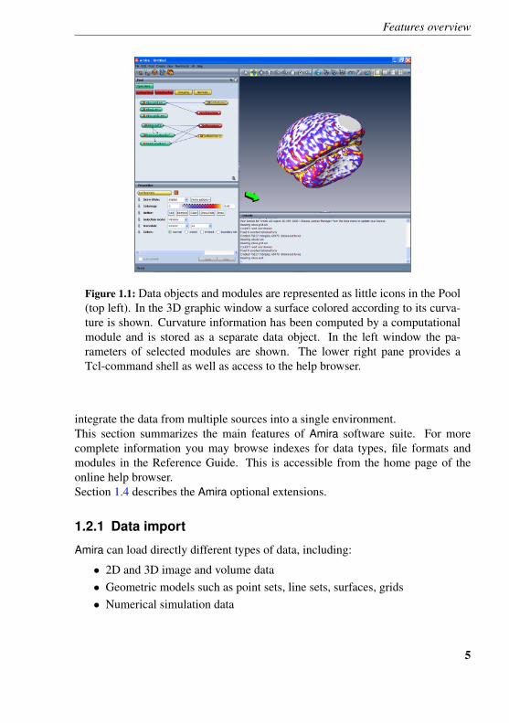
Figure 1.1: Data objects and modules are represented as little icons in the Pool(top left). In the 3D graphic window a surface colored according to its curva-ture is shown. Curvature information has been computed by a computationalmodule and is stored as a separate data object. In the left window the pa-rameters of selected modules are shown. The lower right pane provides aTcl-command shell as well as access to the help browser.
integrate the data from multiple sources into a single environment.This section summarizes the main features of Amira software suite. For morecomplete information you may browse indexes for data types, file formats andmodules in the Reference Guide. This is accessible from the home page of theonline help browser.Section 1.4 describes the Amira optional extensions.
1.2.1 Data import
Amira can load directly different types of data, including:
• 2D and 3D image and volume data• Geometric models such as point sets, line sets, surfaces, grids• Numerical simulation data
5
Chapter 1: Introduction
• Time series and animations
A large number of file formats are supported in the standard edition or throughspecific optional readers. For an introduction to data import, see Chapter 2. Formore details, see section 4.1.
1.2.2 Viewing, navigation, interactivity
All visualization techniques can be arbitrarily combined to produce a single scene.Moreover, multiple data sets can be visualized simultaneously, either in severalviewer windows or in a common one. Thus you can display single or multiple datasets in a single or multiple viewer windows, and navigate freely around or throughthose objects.A built-in spatial transformation editor makes it easy to register data sets withrespect to each other or to deal with different coordinate systems. Automatic reg-istration of volume or geometric data is also possible.Direct interaction with the 3D scene allows you to quickly control regions of in-terest, slices, probes and more.Combinations of data sets, representation and processing features can be definedwith minimal user interaction for simple or complex tasks. See section 1.1.
1.2.3 Visualization of 3D Image Data
1.2.3.1 Slicing and Clipping
You can quickly explore 3D images looking at single or multiple orthographic oroblique sections. Multiple data sets can be superimposed on slices, or displayedas height fields. You can cut away parts of your data to uncover hidden regions.Curved or cylinder slices are also available.
1.2.3.2 Volume Rendering
One of the most intuitive and most powerful techniques for visualizing 3D imagedata is direct volume rendering. Light emission and light absorption parametersare assigned to each point of the volume. Simulating the transmission of lightthrough the volume makes it possible to display your data from any view directionwithout constructing intermediate polygonal models. By exploiting modern graph-ics hardware, Amira is able to perform direct volume rendering in real time, even
6
Features overview
on very large data when using the Very Large Data Option. Thus volume render-ing can instantly highlight relevant features of your data. Volume rendered imagescan be combined with any type of polygonal display. This improves the useful-ness of this technique significantly. Moreover, multiple data sets can be volumerendered simultaneously – a unique feature of Amira. Transfer functions with dif-ferent characteristics required for direct volume rendering can be either generatedautomatically or edited interactively using an intuitive colormap editor.
1.2.3.3 Isosurfaces
Isosurfaces are most commonly used for analyzing arbitrary scalar fields sampledon discrete grids. Applied to 3D images, the method provides a very quick, yetsometimes sufficient method for reconstructing polygonal surface models. Besidestandard algorithms, Amira provides an improved method, which generates signif-icantly fewer triangles with very little computational overhead. In this way, large3D data sets can be displayed interactively even on smaller desktop graphics com-puters.
1.2.3.4 Large Volume Data
With the Very Large Data Option, even very large data sets that cannot be fullyloaded in memory can be manipulated at interactive speed. Multi-resolution tech-niques can manage and visualize extremely large amounts of volume data of upto hundreds of gigabytes. You can then, for instance, quickly select a region ofinterest and extract down-sampled or partial data for further processing.
1.2.4 Image processing
1.2.4.1 Alignment of image slices
The image slice aligner enables you to build a consistent stack of images with man-ual or automatic tools, if, for instance, physical cross-sections have been shiftedduring image acquisition.
1.2.4.2 Image filters
Image features can be enhanced by applying a wide range of filters for control-ling contrast, smoothing, noise reduction and much more. See Image Filters andQuantification+ Option.
7
Chapter 1: Introduction
1.2.4.3 Image segmentation
Segmentation means assigning labels to image voxels that identify and separateobjects in a 3D image. Amira offers a large set of segmentation tools, rangingfrom purely manual to fully automatic: brush (painting), lasso (contouring), magicwand (region growing), thresholding, intelligent scissors, contour fitting (snakes),contour interpolation and extrapolation, wrapping, smoothing and de-noising fil-ters, morphological filters for erosion, dilation, opening and closing operations,connected component analysis, images correlation, objects separation and filter-ing (see Quantification+ Option), etc. See section 2.4 for a tutorial about imagesegmentation.
1.2.5 Model reconstruction
1.2.5.1 Surface generation
Once the interesting features in a 3D image volume have been segmented, Amirais able to create a corresponding polygonal surface model. The surface may havenon-manifold topology if there are locations where three or more regions join.Even in this case the polygonal surface model is guaranteed to be topologicallycorrect, i.e. free of self-intersections. Fractional weights that are automaticallygenerated during segmentation allow the system to produce optionally smoothboundary interfaces. This way realistic high-quality models can be obtained, evenif the underlying image data are of low resolution or contain severe noise artifacts.Making use of innovative acceleration techniques, surface reconstruction can beperformed very quickly. Moreover, the algorithm is robust and fail-safe.
1.2.5.2 Surface Simplification and Editing
Surface simplification is another prominent feature of Amira. It can be used toreduce the number of triangles in an arbitrary surface model according to a user-defined value. Thus, models of finite-element grids, suitable for being processedon low-end machines, can be generated. The underlying simplification algorithmis one of the most elaborate ones available. It is able to preserve topological cor-rectness, i.e., self-intersections commonly produced by other methods are avoided.In addition, the quality of the resulting mesh, according to measures common infinite element analysis, can be controlled. For example, triangles with long edgesor triangles with bad aspect ratio can be suppressed.
8
Features overview
A surface editor is also available for smoothing or refining surface in whole or part,cutting and copying parts of surfaces, defining boundary conditions for furthernumerical simulation, checking and modifying surface triangles.
1.2.5.3 Generation of Tetrahedral Grids
Amira allows you not only to generate surface models from your data but also tocreate true volumetric tetrahedral grids suitable for advanced 3D finite-elementsimulations. These grids are constructed using a flexible advancing-front algo-rithm. Again, special care is taken to obtain meshes of high quality, i.e., tetrahedrawith bad aspect ratio are avoided. Several different file formats are supported, sothat the grid can be exported to many standard simulation packages.
1.2.5.4 Point Clouds/Scattered Data
Amira can also reconstruct surfaces from scattered points (see Delaunay andPointWrap modules).
1.2.5.5 Skeletonization
A set of tools is included for reconstructing and analyzing a dendritic, porous orfracture network from 3D image data.
1.2.6 Visualization of 3D models and numerical data
1.2.6.1 Point sets, line sets
Amira can visualize arbitrary functional data given on 3D point sets or line sets.
1.2.6.2 Polygonal models
A number of drawing styles and coloring schemes help to yield meaningful andinformative visualizations of polygonal models, whether generated from imagedata or imported from CAD or simulation package. Surface and 3D grid meshescan be colored or textured in order to visualize a second independent data set.Another Amira feature comprises the realistic view-dependent way of renderingsemi-transparent surfaces. By correlating transparency with local orientation ofthe surface relative to the viewing direction, complex spatial structures can beunderstood much more easily.
9
Chapter 1: Introduction
1.2.6.3 Numerical data post-processing
Amira allows you to analyze results of numerical simulations. It supports polyg-onal surfaces such as triangular meshes, 3D lattices with uniform, rectilinear ofcurvilinear coordinates, and polyhedral 3D grids such as tetrahedral or hexahedralgrids. Most general purpose image visualization techniques and analysis tools canbe applied, e.g.: slice extraction, computation of isolines or isosurfaces, data prob-ing and histograms. In addition, scalar quantities can be visualized with pseudo-colors on the grid itself.Beside visualization, data representations such as isosurfaces, grid cuts or contourlines can be extracted as first class data objects.Displacement vectors can be visualized on grids or applied as grid deformationthat can be animated.
1.2.6.4 Flow Visualization
Amira provides many advanced tools for vector fields and flow visualization. Vec-tor arrows can be drawn on a slice, within a volume, or upon a surface. Theflow structure may be better revealed by representations such as fast Line IntegralConvolution on slices or arbitrary surfaces, illuminated and animated streamlines,stream ribbons, stream surfaces, particle animations, synthetic vector probe... Allof these stream visualization techniques are highly interactive. While seedpointdistributions can be automatically calculated, you can also select and interactivelymanipulate seed points and structures, thus supporting the investigation the flowfield and highlighting of different features. Amira can also support six-componentcomplex vector fields and phase visualization, e.g. electromagnetic fields.See tutorial section 2.10 (visualization of vector fields).
1.2.6.5 Tensor Data
Amira has support for iconic visualization of tensor field, extraction of eigenvalues,computation of rate of strain tensor, gradient tensor.
1.2.7 General Data Processing and Data Analysis
1.2.7.1 3D registration of multiple data sets
Multiple data sets can be combined to compare images of different objects, or im-ages of an object recorded at different times or with different imaging modalities
10
Features overview
such as X-ray CT and MRI. In addition, fusion of multi-modal data by arbitraryarithmetic operations can be performed to increase the amount of information andaccuracy in the models. Amira allows manual registration through interactive ma-nipulators, automatic rigid or non-rigid registration through landmarks, and auto-matic registration using iterative optimization algorithms (see AffineRegistrationmodule).Surfaces can also be registered using rigid or non-rigid transformations, basedon landmarks sets warping, alignment of centers or principal axes, or distanceminimization algorithms.
1.2.7.2 Operating on 3D data
Many utilities are available for data processing. Here are some important ones. Re-sampling can reduce or enlarge the resolution of a 3D image or data sets defined onregular grids, and different sampling kernels are supported. Data can be cropped orregions of interest can be defined. Data can be converted to any supported primitivetype, from byte to 64-bits floating point numbers. Multi-component data such asmulti-channel images or vector data can be composed or decomposed. Standard3D field operators such as scalar field gradient or vector field curl are available.Surface curvatures and distances between surfaces can also be computed, as scalaror vector information. The powerful Arithmetic module allows to perform calcula-tions on data sets with user-defined expression, and can be used to interpolate databetween regular grids and polyhedral grids. Data sets can also be created fromarithmetic expressions.
1.2.7.3 Measurements, quantification
You can query the exact values of your data sets at arbitrary locations specified in-teractively by a mouse click, or along user-defined lines and spline curves. Probepoints can serve to set interactively isosurfaces. You can plot or export the data forfurther processing with spreadsheet or plotting applications, with probing, mea-suring, counting, and other statistical modules quantify densities, distances, areas,volumes, mean value and standard deviation, ...Histograms of values can be computed and plotted, possibly restricted to a regionof interest. Volume/value diagrams can be also plotted.The Quantification+ Option provides an extensive set of intensity and geometricalmeasurements on image or label data, either for individual labelled particles or asstatistics. See the section dedicated to Quantification+ Option.
11
Chapter 1: Introduction
1.2.8 Matlab integration
You can integrate complex calculus using Matlab software from The Mathworks,Inc. by means of the CalculusMatlab module. This module allows for a connectionto your Matlab server from your Amira session, and executes Matlab computationsdirectly on your Amira data. It is also possible to import and export Matlab matri-ces to and from Amira, and export Amira surfaces to Matlab surfaces. See section2.13.
1.2.9 High Performance Visualization
Amira makes extensive use of graphics hardware for optimal performance and ren-dering quality on your system. Moreover, the Virtual Reality Option allows forcombining multiple graphics engines for high-performance requirements.
1.2.10 Automation, Customization, Extensibility
Tcl scriptingAll Amira components can be controlled via a Tcl command language interface.Tcl scripts are used for saving your work session. Tcl scripts also allow the ad-vanced user to automate or customize tasks with Amira for routine workflows,without the need for C++ programming. Custom Amira modules with user inter-face can even be created as Tcl scripts. Amira module behaviour and 3D interactioncan be customized by using Tcl. Amira can also be used for batch processing.See Chapter 5, including a short introduction to the Tcl scripting language.C++ programmingWith the Virtual Reality Option, Amira can also be extended by programmers. TheDeveloper Option allows for the creation of new custom components for Amirasuch as file readers and writers, computation modules, and even new visualiza-tion modules, using the C++ programming language. New modules and new dataclasses can be defined as subclasses of existing ones. In order to simplify the cre-ation of new custom extensions, a development wizard is included.See the Developer Option User’s Guide for detailed information.
1.3 Application Areas
Amira is successfully being used in a number of different application areas. Amongthese are:
12
Options
• Medicine• Biology• Microscopy• Computational Fluid Dynamics• Neuroscience
Examples from these disciplines are illustrated by several demo scripts containedin the online version of the user’s guide.
1.4 Options
Amira Options are additional sets of modules providing solutions for dedicatedapplication areas. Options can be added to a standard Amira installation at anytime. For each option a separate license is required. Currently, the followingoptions are available for Amira:
• Amira Developer Option allows you to develop your own custom modules,file readers, and file writers using the C++ programming language.
• Amira Molecular Option adds advanced tools for the visualization ofmolecules. It combines Amira’s strong capabilities for 3D data visualiza-tion such as hardware-accelerated volume rendering, with specific tools formolecular visualization and data analysis, such as molecular surfaces, se-quence alignment, configuration density computation, and molecule trajec-tories. Amira Molecular Option includes a very powerful molecule editor.
• Amira Mesh Option supports mesh generation for flow, stress, and ther-mal analysis; for export of surface or 3D meshes to solvers; and for post-processing of data coming back from these solvers, providing very powerfulvisualization on scalar, vector, and tensor fields.
• Amira DICOM reader allows for import/export of DICOM data in Amira,making Amira the perfect application for medical data analysis.
• Amira Microscopy Option includes readers for most important microscopyfile formats, 3D image deconvolution and and a dedicated filament editor.
13
Chapter 1: Introduction
• Amira Skeleton Option supports reconstruction and analysis of porous,vascular and dendritic networks.
• Amira Virtual Reality Option is designed to enable the use of Amira’s ad-vanced data visualization and analysis features on immersive VR systemsand tiled screen configurations. It has built-in support for efficient multi-threaded rendering on multipipe systems and for distributed rendering oncluster systems using application-level distribution. This approach leads tooptimal performance with minimal bandwidth requirements. Tracking ca-pabilities allow for a true immersive experience as well as interaction withthe visualization.
• Amira Very Large Data Option manages and visualizes very large amountsof volume data, up to hundreds of gigabytes. The multi-resolution tech-nique used in this option allows for interactive visualization and navigationthrough vast amounts of data.
• Amira Quantification+ Option includes new image processing capabilityas well as image analysis and quantification tools. Very powerful for ma-terial sciences, this option allows for efficient statistical analysis of data inthis application area.
• Specialized Readers For the following file formats / applications special-ized readers are available: SEG-Y, CATIA 4, CATIA 5, IGES, STEP,TNO Madymo, and Mecalog Radioss
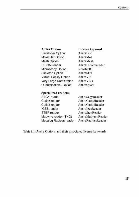
Table 1.1 shows the license keyword associated with each of the Amira Options.For additional information about Amira and its options, please refer to the Amiraweb site, http://www.amira.com/.
14
Options
Amira Option License keywordDeveloper Option AmiraDevMolecular Option AmiraMolMesh Option AmiraMeshDICOM reader AmiraDicomReaderMicroscopy Option ResolveRTSkeleton Option AmiraSkelVirtual Reality Option AmiraVRVery Large Data Option AmiraVLDQuantification+ Option AmiraQuant
Specialized readers:SEGY reader AmiraSegyReaderCatia5 reader AmiraCatia5ReaderCatia4 reader AmiraCatia4ReaderIGES reader AmiraIgesReaderSTEP reader AmiraStepReaderMadymo reader (TNO) AmiraMadymoReaderMecalog Radioss reader AmiraRadiossReader
Table 1.1: Amira Options and their associated license keywords
15

2 First steps in Amira
This chapter contains step-by-step tutorials illustrating the use of Amira. The tuto-rials are almost independent of each other, so after reading the basics in the GettingStarted section it is possible to follow each tutorial without knowing the others. Ifyou go through all tutorials you will get a good survey of Amira’s basic features.In particular, these topics will be covered:
• Getting started - the basics of Amira
• Reading images - how to read images• Visualizing 3D images - slices, isosurfaces, volume rendering• Image segmentation - segmentation of 3D image data• Surface reconstruction - surface reconstruction from 3D images• Grid generation - creating a tetrahedral grid from a triangular surface• Warping - how to work with landmark sets• 3D image registration - how to register 3D image data sets• Alignment of 2D Physical Cross-Sections - how to reconstruct a 3D model• Vector fields - stream lines and other techniques• Filament Editor - filament tracing for neurons and vessels images• The DemoMaker module - creating animations with the DemoMaker mod-
ule• Creating movie files - how to use the MovieMaker module• Using MATLAB - how to use the CalculusMatlab module• Trace Filaments - how to extract a network model from a neuron 3D image
data• Multi-planar Viewer - visualize and register multiple volumes
In all tutorials the steps to be performed by the user are marked by a dot. Ifyou only want to get a quick idea how to work with Amira you may skip theexplanations between successive steps and just follow the instructions. But inorder to get a deeper understanding you should refer to the text.
17
Chapter 2: First steps in Amira
Note: If you want to visualize your own data, please first refer to Section 4.1. Thissection contains some general hints on how to import data sets into Amira.Note for Mac users: Please read Section 4.7 before starting the tutorials.
2.1 Getting Started
In this section you will learn how to
1. start the program2. load a demo data set into the system3. invoke editors for editing the data4. connect visualization modules to the data5. interact with the 3D viewer.
The following text has the form of a short step-by-step tutorial. Each step buildson the steps described before. We recommend that you read the text online andcarry out the instructions directly on the computer. Instructions are indicated by adot so you can execute them quickly without reading the explanations between theinstructions.
• Windows, select the Amira icon from the start menu.• Mac, select the Amira icon from the Application menu.• Unix-Linux, start Amira by entering Amira in a shell window.
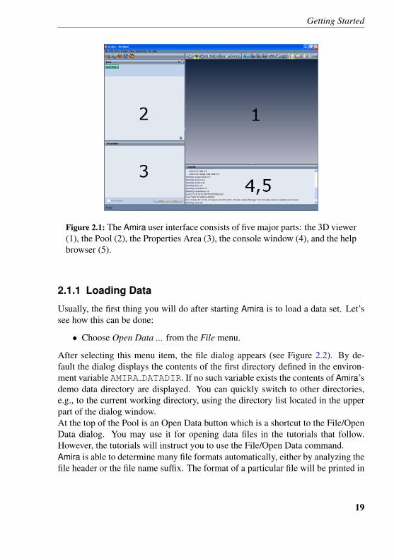
If there is no such command, the software has not been properly installed. In thiscase try to execute the script bin/start located in the AMIRA ROOT directory.When Amira is running, a window like the one shown in Figure 2.1 appears on thescreen. The user interface is divided into four major regions. The 3D viewer win-dow displays visualization results, e.g., slices or isosurfaces. The Pool will containsmall icons representing data objects and modules. The Properties Area displaysinterface elements (ports) associated with Amira objects. Finally, the lower leftpane is shared by the console and Amira’s integrated hypertext help browser. Clickon the Console or Help tab to select which window you want to view. The consoleprints system messages and lets you enter Amira commands. You can use the helpbrowser to read the user’s guide online.You can also activate the help browser by pressing F1, selecting User’s Guide fromthe Help menu of Amira’s main window, or by typing help in the console window.
18
Getting Started
Figure 2.1: The Amira user interface consists of five major parts: the 3D viewer(1), the Pool (2), the Properties Area (3), the console window (4), and the helpbrowser (5).
2.1.1 Loading Data
Usually, the first thing you will do after starting Amira is to load a data set. Let’ssee how this can be done:
• Choose Open Data ... from the File menu.
After selecting this menu item, the file dialog appears (see Figure 2.2). By de-fault the dialog displays the contents of the first directory defined in the environ-ment variable AMIRA DATADIR. If no such variable exists the contents of Amira’sdemo data directory are displayed. You can quickly switch to other directories,e.g., to the current working directory, using the directory list located in the upperpart of the dialog window.At the top of the Pool is an Open Data button which is a shortcut to the File/OpenData dialog. You may use it for opening data files in the tutorials that follow.However, the tutorials will instruct you to use the File/Open Data command.Amira is able to determine many file formats automatically, either by analyzing thefile header or the file name suffix. The format of a particular file will be printed in
19
Chapter 2: First steps in Amira
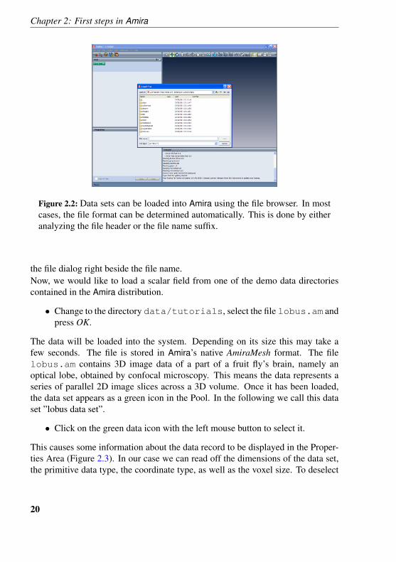
Figure 2.2: Data sets can be loaded into Amira using the file browser. In mostcases, the file format can be determined automatically. This is done by eitheranalyzing the file header or the file name suffix.
the file dialog right beside the file name.Now, we would like to load a scalar field from one of the demo data directoriescontained in the Amira distribution.
• Change to the directory data/tutorials, select the file lobus.am andpress OK.
The data will be loaded into the system. Depending on its size this may take afew seconds. The file is stored in Amira’s native AmiraMesh format. The filelobus.am contains 3D image data of a part of a fruit fly’s brain, namely anoptical lobe, obtained by confocal microscopy. This means the data represents aseries of parallel 2D image slices across a 3D volume. Once it has been loaded,the data set appears as a green icon in the Pool. In the following we call this dataset ”lobus data set”.
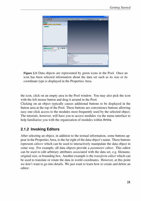
• Click on the green data icon with the left mouse button to select it.
This causes some information about the data record to be displayed in the Proper-ties Area (Figure 2.3). In our case we can read off the dimensions of the data set,the primitive data type, the coordinate type, as well as the voxel size. To deselect
20
Getting Started
Figure 2.3: Data objects are represented by green icons in the Pool. Once anicon has been selected information about the data set such as its size or itscoordinate type is displayed in the Properties Area.
the icon, click on an empty area in the Pool window. You may also pick the iconwith the left mouse button and drag it around in the Pool.Clicking on an object typically causes additional buttons to be displayed in thebutton area at the top of the Pool. These buttons are convenience buttons allowingeasy one-click access to the modules most frequently used by the selected object.The tutorials, however, will have you to access modules via the menu interface tohelp familiarize you with the organization of modules within Amira.
2.1.2 Invoking Editors
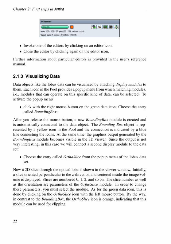
After selecting an object, in addition to the textual information, some buttons ap-pear in the Properties Area, to the far right of the data object’s name. These buttonsrepresent editors which can be used to interactively manipulate the data object insome way. For example, all data objects provide a parameter editor. This editorcan be used to edit arbitrary attributes associated with the data set, e.g. filename,original size, or bounding box. Another example is the transform editor which canbe used to translate or rotate the data in world coordinates. However, at this pointwe don’t want to go into details. We just want to learn how to create and delete aneditor:
21
Chapter 2: First steps in Amira
• Invoke one of the editors by clicking on an editor icon.• Close the editor by clicking again on the editor icon.
Further information about particular editors is provided in the user’s referencemanual.
2.1.3 Visualizing Data
Data objects like the lobus data can be visualized by attaching display modules tothem. Each icon in the Pool provides a popup menu from which matching modules,i.e., modules that can operate on this specific kind of data, can be selected. Toactivate the popup menu
• click with the right mouse button on the green data icon. Choose the entrycalled BoundingBox.
After you release the mouse button, a new BoundingBox module is created andis automatically connected to the data object. The Bounding Box object is rep-resented by a yellow icon in the Pool and the connection is indicated by a blueline connecting the icons. At the same time, the graphics output generated by theBoundingBox module becomes visible in the 3D viewer. Since the output is notvery interesting, in this case we will connect a second display module to the dataset:
• Choose the entry called OrthoSlice from the popup menu of the lobus dataset.
Now a 2D slice through the optical lobe is shown in the viewer window. Initially,a slice oriented perpendicular to the z-direction and centered inside the image vol-ume is displayed. Slices are numbered 0, 1, 2, and so on. The slice number as wellas the orientation are parameters of the OrthoSlice module. In order to changethese parameters, you must select the module. As for the green data icon, this isdone by clicking on the OrthoSlice icon with the left mouse button. By the way,in contrast to the BoundingBox, the OrthoSlice icon is orange, indicating that thismodule can be used for clipping.
22
Getting Started
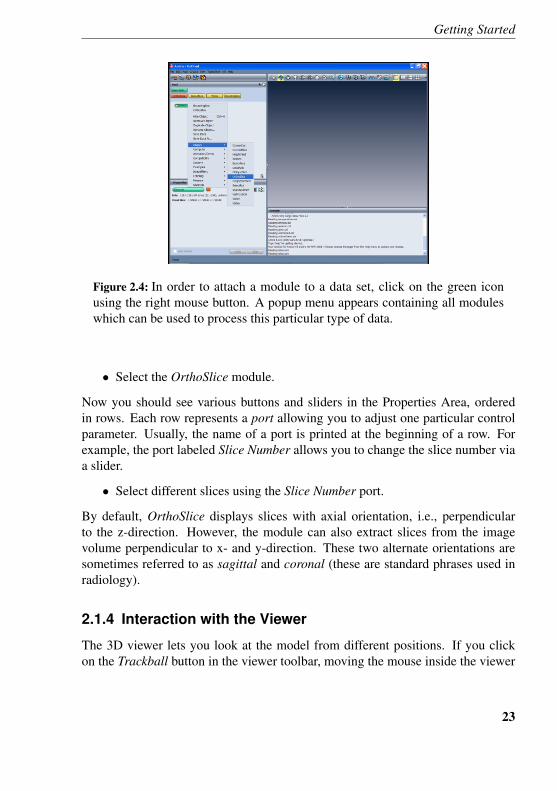
Figure 2.4: In order to attach a module to a data set, click on the green iconusing the right mouse button. A popup menu appears containing all moduleswhich can be used to process this particular type of data.
• Select the OrthoSlice module.
Now you should see various buttons and sliders in the Properties Area, orderedin rows. Each row represents a port allowing you to adjust one particular controlparameter. Usually, the name of a port is printed at the beginning of a row. Forexample, the port labeled Slice Number allows you to change the slice number viaa slider.
• Select different slices using the Slice Number port.
By default, OrthoSlice displays slices with axial orientation, i.e., perpendicularto the z-direction. However, the module can also extract slices from the imagevolume perpendicular to x- and y-direction. These two alternate orientations aresometimes referred to as sagittal and coronal (these are standard phrases used inradiology).
2.1.4 Interaction with the Viewer
The 3D viewer lets you look at the model from different positions. If you clickon the Trackball button in the viewer toolbar, moving the mouse inside the viewer
23
Chapter 2: First steps in Amira
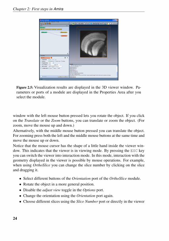
Figure 2.5: Visualization results are displayed in the 3D viewer window. Pa-rameters or ports of a module are displayed in the Properties Area after youselect the module.
window with the left mouse button pressed lets you rotate the object. If you clickon the Translate or the Zoom buttons, you can translate or zoom the object. (Forzoom, move the mouse up and down.)Alternatively, with the middle mouse button pressed you can translate the object.For zooming press both the left and the middle mouse buttons at the same time andmove the mouse up or down.Notice that the mouse cursor has the shape of a little hand inside the viewer win-dow. This indicates that the viewer is in viewing mode. By pressing the ESC keyyou can switch the viewer into interaction mode. In this mode, interaction with thegeometry displayed in the viewer is possible by mouse operations. For example,when using OrthoSlice you can change the slice number by clicking on the sliceand dragging it.
• Select different buttons of the Orientation port of the OrthoSlice module.• Rotate the object in a more general position.• Disable the adjust view toggle in the Options port.• Change the orientation using the Orientation port again.• Choose different slices using the Slice Number port or directly in the viewer
24
Getting Started
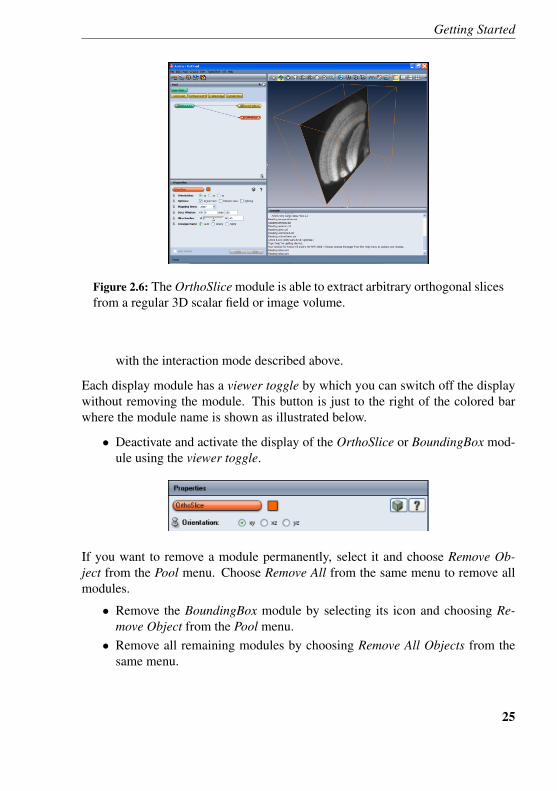
Figure 2.6: The OrthoSlice module is able to extract arbitrary orthogonal slicesfrom a regular 3D scalar field or image volume.
with the interaction mode described above.
Each display module has a viewer toggle by which you can switch off the displaywithout removing the module. This button is just to the right of the colored barwhere the module name is shown as illustrated below.
• Deactivate and activate the display of the OrthoSlice or BoundingBox mod-ule using the viewer toggle.
If you want to remove a module permanently, select it and choose Remove Ob-ject from the Pool menu. Choose Remove All from the same menu to remove allmodules.
• Remove the BoundingBox module by selecting its icon and choosing Re-move Object from the Pool menu.
• Remove all remaining modules by choosing Remove All Objects from thesame menu.
25
Chapter 2: First steps in Amira
Now the Pool should be empty again. You may continue with the next tutorial, i.e.,the one on scalar field visualization.
2.2 How to load image data
Loading image data is one of the most basic operations in Amira. Other than with2D images, there are not many standardized file formats containing 3D images.This tutorial guides you by means of examples on how to load the different kindsof 3D images into Amira. In particular this tutorial covers the following topics:
1. Using the File/Open Data... browser and setting the file format.2. Reading 3D image data from multiple 2D slices.3. Setting the bounding box or voxel size of 3D images.4. The Stacked Slices file format.5. Working with LargeDiskData.
2.2.1 The Amira File Browser
Image data is loaded in Amira with the File/Open Data... dialog. All file formatssupported by Amira are recognized automatically either by a data header or by thefile name suffix. What follows is only of concern in these cases:
• The automatic file format detection fails.• 3D image data is stored in several 2D files.• The data is larger than the available main memory.
Setting the file formatIn most cases the format of a file is determined automatically, either by checkingthe file header or by comparing the file name suffix with a list of known suffixes.In the load dialog the file format is displayed in a separate column in detail view.
Example:
• Files containing the string AmiraMesh in the first line are considered Ami-raMesh files.
• Files with the suffix .stl are considered STL files.
26
How to load image data
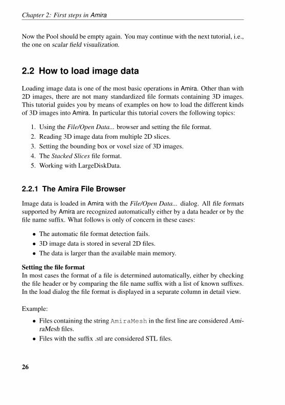
Figure 2.7: The Format option of the file browser
If automatic file format detection fails, e.g. because some non-standard suffix hasbeen used, the format may be set manually using the Format entry in the pop-upmenu of the Load dialog (right mouse button).
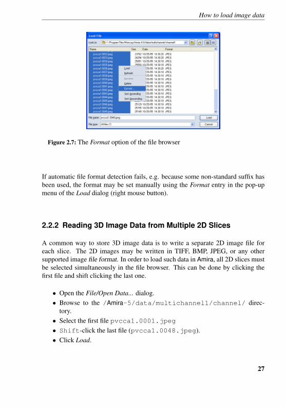
2.2.2 Reading 3D Image Data from Multiple 2D Slices
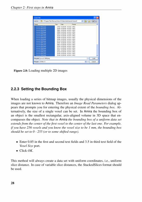
A common way to store 3D image data is to write a separate 2D image file foreach slice. The 2D images may be written in TIFF, BMP, JPEG, or any othersupported image file format. In order to load such data in Amira, all 2D slices mustbe selected simultaneously in the file browser. This can be done by clicking thefirst file and shift clicking the last one.
• Open the File/Open Data... dialog.• Browse to the /Amira-5/data/multichannel1/channel/ direc-
tory.• Select the first file pvcca1.0001.jpeg• Shift-click the last file (pvcca1.0048.jpeg).• Click Load.
27
Chapter 2: First steps in Amira
Figure 2.8: Loading multiple 2D images
2.2.3 Setting the Bounding Box
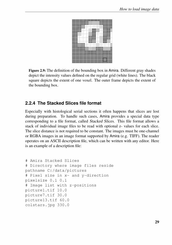
When loading a series of bitmap images, usually the physical dimensions of theimages are not known to Amira. Therefore an Image Read Parameters dialog ap-pears that prompts you for entering the physical extent of the bounding box. Al-ternatively, the size of a single voxel can be set. In Amira the bounding box ofan object is the smallest rectangular, axis-aligned volume in 3D space that en-compasses the object. Note that in Amira the bounding box of a uniform data setextends from the center of the first voxel to the center of the last one. For example,if you have 256 voxels and you know the voxel size to be 1 mm, the bounding boxshould be set to 0 - 255 (or to some shifted range).
• Enter 0.85 in the first and second text fields and 3.5 in third text field of theVoxel Size port.
• Click OK.
This method will always create a data set with uniform coordinates, i.e., uniformslice distance. In case of variable slice distances, the StackedSlices format shouldbe used.
28
How to load image data
Figure 2.9: The definition of the bounding box in Amira. Different gray shadesdepict the intensity values defined on the regular grid (white lines). The blacksquare depicts the extent of one voxel. The outer frame depicts the extent ofthe bounding box.
2.2.4 The Stacked Slices file format
Especially with histological serial sections it often happens that slices are lostduring preparation. To handle such cases, Amira provides a special data typecorresponding to a file format, called Stacked Slices. This file format allows astack of individual image files to be read with optional z- values for each slice.The slice distance is not required to be constant. The images must be one-channelor RGBA images in an image format supported by Amira (e.g. TIFF). The readeroperates on an ASCII description file, which can be written with any editor. Hereis an example of a description file:
# Amira Stacked Slices# Directory where image files residepathname C:/data/pictures# Pixel size in x- and y-directionpixelsize 0.1 0.1# Image list with z-positionspicture1.tif 10.0picture7.tif 30.0picture13.tif 60.0colstars.jpg 330.0
29
Chapter 2: First steps in Amira
end
Some remarks on the syntax:
• # Amira Stacked Slices is an optional header that allows Amira toautomatically determine the file format.
• pathname is optional and can be included if the pictures are not in thesame directory as the description file. A space separates the tag ”pathname”from the actual pathname.
• pixelsize is optional, too. The statement specifies the pixel size in x-and y-directions. The bounding box of the resulting 3D image is set from 0to pixelsize*(number of pixels-1).
• picture1.tif 10.0 is the name of the slice and its z-value, separatedby a space character.
• end indicates the end of the description file.• Comments are indicated by a hash-mark character (#).
2.2.5 Working with Large Disk Data
Sometimes image data are so large that they do not fit into the main memory of thecomputer. Since the Amira visualization modules rely on the fact that data are inphysical memory, this would mean that such data cannot be displayed in Amira. Toovercome this, a special purpose module is provided that leaves most of the dataon disk and retrieves only a user-specified subvolume. This subvolume can thenbe visualized with the standard visualization modules in Amira.
• Use the File/Open Data... dialog and go to c:/Program Files/Amira-5/data/medical/
• Right-click on the reg005.ctdata.am and select the Format entry from thepop-up dialog
• Select AmiraMesh as LargeDiskData as format and confirm your choicewith OK.
• Press the Load button.
The data will be displayed in the Pool as a regular green data icon. The info lineindicates that it belongs to the data class HxRawAsExternalData.
• Right mouse click, attach a BoundingBox module.
30
How to load image data
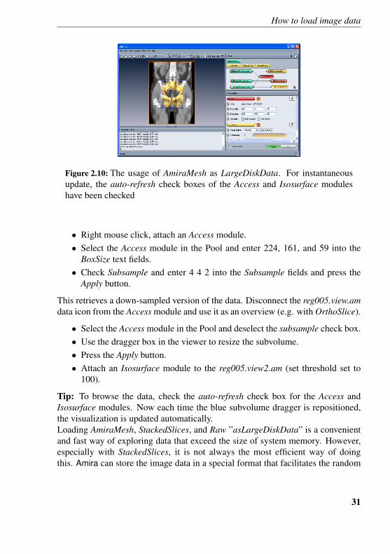
Figure 2.10: The usage of AmiraMesh as LargeDiskData. For instantaneousupdate, the auto-refresh check boxes of the Access and Isosurface moduleshave been checked
• Right mouse click, attach an Access module.• Select the Access module in the Pool and enter 224, 161, and 59 into the
BoxSize text fields.• Check Subsample and enter 4 4 2 into the Subsample fields and press the
Apply button.
This retrieves a down-sampled version of the data. Disconnect the reg005.view.amdata icon from the Access module and use it as an overview (e.g. with OrthoSlice).
• Select the Access module in the Pool and deselect the subsample check box.• Use the dragger box in the viewer to resize the subvolume.• Press the Apply button.• Attach an Isosurface module to the reg005.view2.am (set threshold set to
100).
Tip: To browse the data, check the auto-refresh check box for the Access andIsosurface modules. Now each time the blue subvolume dragger is repositioned,the visualization is updated automatically.Loading AmiraMesh, StackedSlices, and Raw ”asLargeDiskData” is a convenientand fast way of exploring data that exceed the size of system memory. However,especially with StackedSlices, it is not always the most efficient way of doingthis. Amira can store the image data in a special format that facilitates the random
31
Chapter 2: First steps in Amira
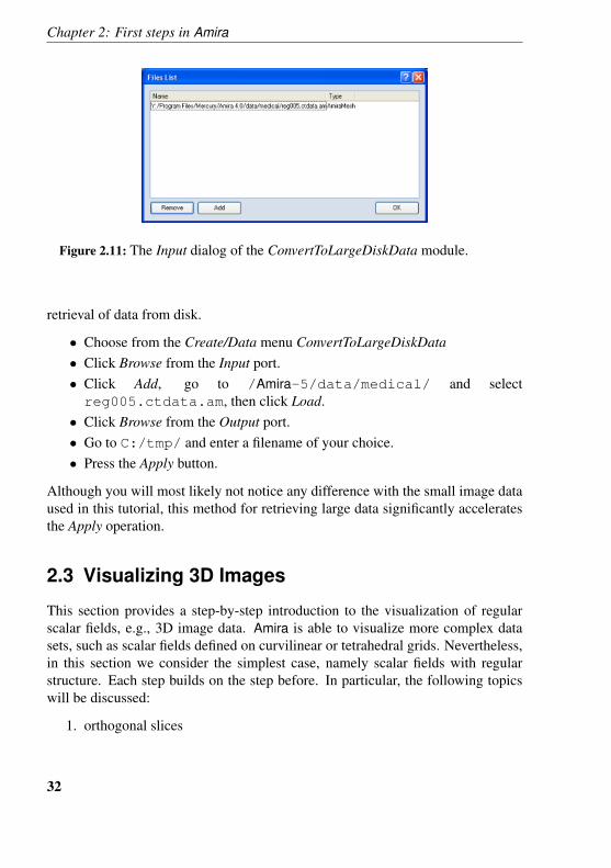
Figure 2.11: The Input dialog of the ConvertToLargeDiskData module.
retrieval of data from disk.
• Choose from the Create/Data menu ConvertToLargeDiskData• Click Browse from the Input port.• Click Add, go to /Amira-5/data/medical/ and selectreg005.ctdata.am, then click Load.
• Click Browse from the Output port.• Go to C:/tmp/ and enter a filename of your choice.• Press the Apply button.
Although you will most likely not notice any difference with the small image dataused in this tutorial, this method for retrieving large data significantly acceleratesthe Apply operation.
2.3 Visualizing 3D Images
This section provides a step-by-step introduction to the visualization of regularscalar fields, e.g., 3D image data. Amira is able to visualize more complex datasets, such as scalar fields defined on curvilinear or tetrahedral grids. Nevertheless,in this section we consider the simplest case, namely scalar fields with regularstructure. Each step builds on the step before. In particular, the following topicswill be discussed:
1. orthogonal slices
32
Visualizing 3D Images
2. simple threshold segmentation3. resampling the data4. displaying an isosurface5. cropping the data6. volume rendering
We start by loading the data you already know from Section 2.1 (Getting Started):a 3D image data set of a part of a fruit fly’s brain. The data set has been recordedwith a confocal laser scanning microscope at the University of Wuerzburg.
• Load the file lobus.am located in subdirectory data/tutorials.
2.3.1 Orthogonal Slices
The fastest and in many cases most ”standard” way of visualizing 3D image data isby extracting orthogonal slices from the 3D data set. Amira allows you to displaymultiple slices with different orientations simultaneously within a single viewer.
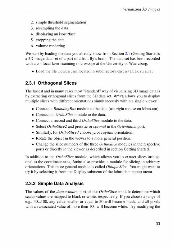
• Connect a BoundingBox module to the data (use right mouse on lobus.am).• Connect an OrthoSlice module to the data.• Connect a second and third OrthoSlice module to the data.• Select OrthoSlice2 and press xz or coronal in the Orientation port.• Similarly, for OrthoSlice3 choose yz or sagittal orientation.• Rotate the object in the viewer to a more general position.• Change the slice numbers of the three OrthoSlice modules in the respective
ports or directly in the viewer as described in section Getting Started.
In addition to the OrthoSlice module, which allows you to extract slices orthog-onal to the coordinate axes, Amira also provides a module for slicing in arbitraryorientations. This more general module is called ObliqueSlice. You might want totry it by selecting it from the Display submenu of the lobus data popup menu.
2.3.2 Simple Data Analysis
The values of the data window port of the OrthoSlice module determine whichscalar values are mapped to black or white, respectively. If you choose a range ofe.g., 30...100, any value smaller or equal to 30 will become black, and all pixelswith an associated value of more then 100 will become white. Try modifying the
33
Chapter 2: First steps in Amira
Figure 2.12: Lobus data set visualized using three orthogonal slices.
range. This port provides a simple way of determining a threshold, which latercan be used for segmentation, e.g., in biology or medicine to separate backgroundpixels from anatomical structures. This can be most easily done by making theminimum and maximum values coincide.
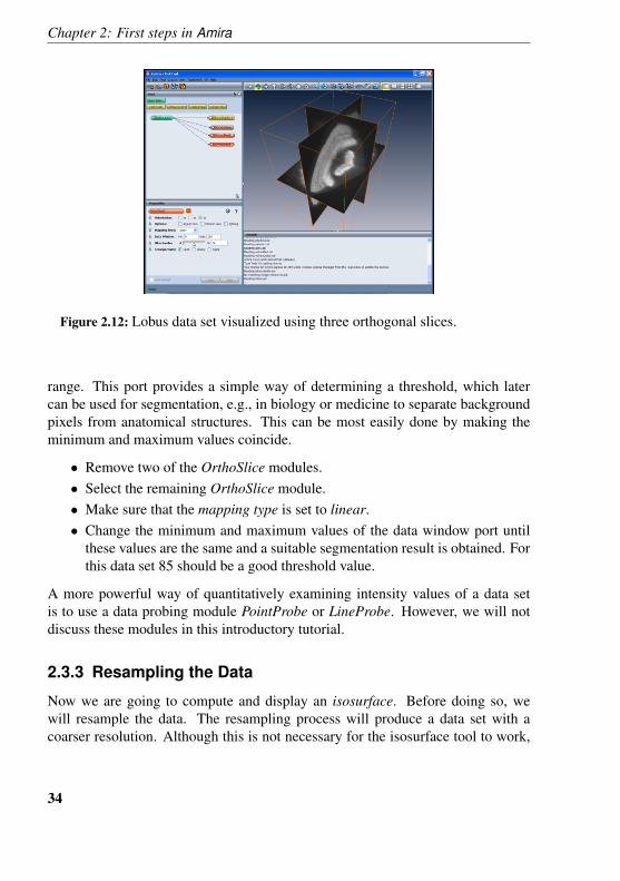
• Remove two of the OrthoSlice modules.• Select the remaining OrthoSlice module.• Make sure that the mapping type is set to linear.• Change the minimum and maximum values of the data window port until
these values are the same and a suitable segmentation result is obtained. Forthis data set 85 should be a good threshold value.
A more powerful way of quantitatively examining intensity values of a data setis to use a data probing module PointProbe or LineProbe. However, we will notdiscuss these modules in this introductory tutorial.
2.3.3 Resampling the Data
Now we are going to compute and display an isosurface. Before doing so, wewill resample the data. The resampling process will produce a data set with acoarser resolution. Although this is not necessary for the isosurface tool to work,
34
Visualizing 3D Images
Figure 2.13: By adjusting the data window of the OrthoSlice module a suitablevalue for threshold segmentation can be found. Intensity values smaller thanthe min value will be mapped to black, intensity values bigger than the maxvalue will be mapped to white.
it decreases computation time and improves rendering performance. In addition,you will get acquainted with another type of module. The Resample module isa computational module. Computational modules are represented by red icons.Typically you must press the green Apply button at the bottom of the PropertiesArea to start the computation. After you press this button they produce a new dataobject containing the result.
• Connect a Resample module to the data and select it.• Enter values for a coarser resolution, e.g., x=64, y=64, z=43.• Press the Apply button.
A new green data icon representing the output of the resample computation namedlobus.Resampled is created. You can treat this new data set like the original lobusdata. In the popup menu of the resampled lobus you will find exactly the sameattachable modules and you can save and load it like the original data.You may want to compare the resampled data set with the original one using theOrthoSlice module. You can simply pick the blue line indicating the data connec-tion and drag it to a different data source. Whenever the mouse pointer is over a
35
Chapter 2: First steps in Amira
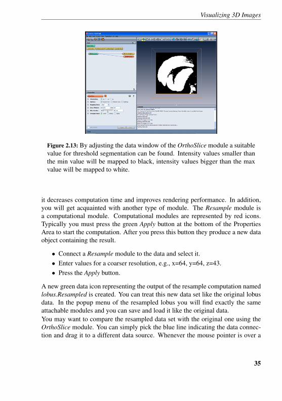
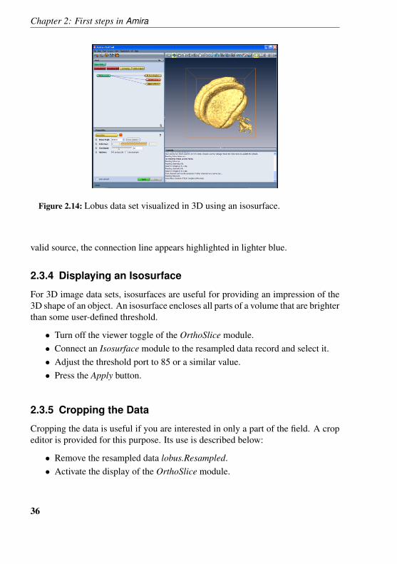
Figure 2.14: Lobus data set visualized in 3D using an isosurface.
valid source, the connection line appears highlighted in lighter blue.
2.3.4 Displaying an Isosurface
For 3D image data sets, isosurfaces are useful for providing an impression of the3D shape of an object. An isosurface encloses all parts of a volume that are brighterthan some user-defined threshold.
• Turn off the viewer toggle of the OrthoSlice module.• Connect an Isosurface module to the resampled data record and select it.• Adjust the threshold port to 85 or a similar value.• Press the Apply button.
2.3.5 Cropping the Data
Cropping the data is useful if you are interested in only a part of the field. A cropeditor is provided for this purpose. Its use is described below:
• Remove the resampled data lobus.Resampled.• Activate the display of the OrthoSlice module.
36
Visualizing 3D Images
• Select the lobus.am data icon.• Click on the Crop Editor button in the Properties Area.
A new window pops up. There are two ways to crop the data set. You can eithertype the desired ranges of x, y, and z coordinates into the crop editor’s windowor put the viewer into interaction mode and adjust the crop box using the greenhandles directly in the viewer window.
• Put the viewer into interaction mode.• With the left mouse button, pick one of the green handles attached to the
crop volume. Drag and transform the volume until the part of the data youare interested in is included.
• Press OK in the crop editor’s dialog window.
The new dimensions of the data set are given in the Properties Area. If you want towork with this cropped data record in later sessions you should save it by choosingSave Data As ... from the File menu.As you already might have noticed, the crop editor also allows you to rescale thebounding box of the data set. By changing the bounding box alone, no voxelswill be cropped. You may also use the crop editor to enlarge the data set, e.g., byentering a negative value for the k min number. In this case the first slice of thedata set will be duplicated as many times as necessary. Also, the bounding boxwill be updated automatically.
2.3.6 Volume Rendering
Volume Rendering is a visualization technique that gives a 3D impression of thewhole data set without segmentation. The underlying model is based on the emis-sion and absorption of light that pertains to every voxel of the view volume. Thealgorithm simulates the casting of light rays through the volume from pre-setsources. It determines how much light reaches each voxel on the ray and is emit-ted or absorbed by the voxel. Then it computes what can be seen from the currentviewing point as implied by the current placement of the volume relative to theviewing plane, simulating the casting of sight rays through the volume from theviewing point.You can choose between two different methods for these computations: maximumintensity projections or an ordinary emission-absorption model.
• Remove all objects in the Pool other than the lobus.am data record.
37
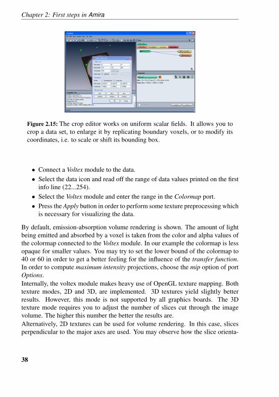
Chapter 2: First steps in Amira
Figure 2.15: The crop editor works on uniform scalar fields. It allows you tocrop a data set, to enlarge it by replicating boundary voxels, or to modify itscoordinates, i.e. to scale or shift its bounding box.
• Connect a Voltex module to the data.• Select the data icon and read off the range of data values printed on the first
info line (22...254).• Select the Voltex module and enter the range in the Colormap port.• Press the Apply button in order to perform some texture preprocessing which
is necessary for visualizing the data.
By default, emission-absorption volume rendering is shown. The amount of lightbeing emitted and absorbed by a voxel is taken from the color and alpha values ofthe colormap connected to the Voltex module. In our example the colormap is lessopaque for smaller values. You may try to set the lower bound of the colormap to40 or 60 in order to get a better feeling for the influence of the transfer function.In order to compute maximum intensity projections, choose the mip option of portOptions.Internally, the voltex module makes heavy use of OpenGL texture mapping. Bothtexture modes, 2D and 3D, are implemented. 3D textures yield slightly betterresults. However, this mode is not supported by all graphics boards. The 3Dtexture mode requires you to adjust the number of slices cut through the imagevolume. The higher this number the better the results are.Alternatively, 2D textures can be used for volume rendering. In this case, slicesperpendicular to the major axes are used. You may observe how the slice orienta-
38
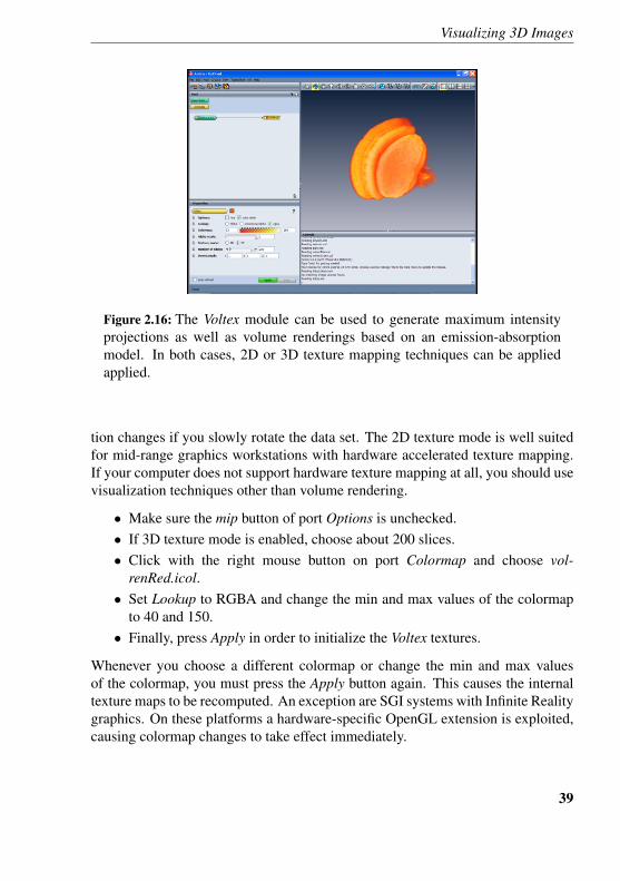
Visualizing 3D Images
Figure 2.16: The Voltex module can be used to generate maximum intensityprojections as well as volume renderings based on an emission-absorptionmodel. In both cases, 2D or 3D texture mapping techniques can be appliedapplied.
tion changes if you slowly rotate the data set. The 2D texture mode is well suitedfor mid-range graphics workstations with hardware accelerated texture mapping.If your computer does not support hardware texture mapping at all, you should usevisualization techniques other than volume rendering.
• Make sure the mip button of port Options is unchecked.• If 3D texture mode is enabled, choose about 200 slices.• Click with the right mouse button on port Colormap and choose vol-
renRed.icol.• Set Lookup to RGBA and change the min and max values of the colormap
to 40 and 150.• Finally, press Apply in order to initialize the Voltex textures.
Whenever you choose a different colormap or change the min and max valuesof the colormap, you must press the Apply button again. This causes the internaltexture maps to be recomputed. An exception are SGI systems with Infinite Realitygraphics. On these platforms a hardware-specific OpenGL extension is exploited,causing colormap changes to take effect immediately.
39
Chapter 2: First steps in Amira
2.4 Segmentation of 3D Images
By following this step-by-step tutorial you will learn how to interactively create asegmentation of a 3D image. A segmentation assigns to each pixel of the imagea label describing to which region or material the pixel belongs, e.g., bone or thekidney. The segmentation is stored in a separate data object called a LabelField. Asegmentation is the prerequisite for surface model generation or accurate volumemeasurement.This tutorial comprises the following steps:
1. Creation of an empty LabelField.2. Interactive editing of the labels in the Image Segmentation Editor.3. Measuring the volume of the segmented structures.4. An alternative segmentation method: Threshold segmentation.
2.4.1 Interactive Image Segmentation
• Load the lobus.am data file from the directory data/tutorials.• Right click on the green icon and choose LabelField from the Labelling
section.
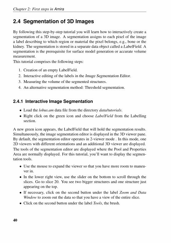
A new green icon appears, the LabelField that will hold the segmentation results.Simultaneously, the image segmentation editor is displayed in the 3D viewer pane.By default, the segmentation editor operates in 2-viewer mode . In this mode, one2D viewers with different orientations and an additional 3D viewer are displayed.The tools of the segmentation editor are displayed where the Pool and PropertiesArea are normally displayed. For this tutorial, you’ll want to display the segmen-tation tools.
• Use the mouse to expand the viewer so that you have more room to maneu-ver in.
• In the lower right view, use the slider on the bottom to scroll through theslices. Go to slice 20. You see two bigger structures and one structure justappearing on the top.
• If necessary, click on the second button under the label Zoom and DataWindow to zoom out the data so that you have a view of the entire slice.
• Click on the second button under the label Tools, the brush.
40
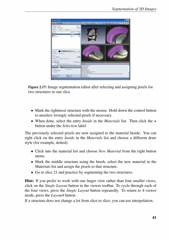
Segmentation of 3D Images
Figure 2.17: Image segmentation editor after selecting and assigning pixels fortwo structures in one slice
• Mark the rightmost structure with the mouse. Hold down the control buttonto unselect wrongly selected pixels if necessary.
• When done, select the entry Inside in the Materials list. Then click the +button under the Selection label.
The previously selected pixels are now assigned to the material Inside. You canright click on the entry Inside in the Materials list and choose a different drawstyle (for example, dotted).
• Click into the material list and choose New Material from the right buttonmenu.
• Mark the middle structure using the brush, select the new material in theMaterials list and assign the pixels to that structure.
• Go to slice 21 and practice by segmenting the two structures.
Hint: If you prefer to work with one larger view rather than four smaller views,click on the Single Layout button in the viewer toolbar. To cycle through each ofthe four views, press the Single Layout button repeatedly. To return to 4-viewermode, press the Layout4 button.If a structure does not change a lot from slice to slice, you can use interpolation.
41
Chapter 2: First steps in Amira
• Go to slice 22 and mark the right structure using the brush. Go to slice 31and mark the same structure.
• Choose from the menu bar: Selection/Interpolate.• Scroll through the data set. You should see that the in between slices 23 to
30 are selected too.• In order to assign the selected pixels in all slices to the Inside material, select
the Inside material in the list, then click the + button.
• Repeat the procedure between slice 32 and 50.• Repeat the procedure for the middle structure.
Hints:
• It is highly recommended to frequently save the segmentation results whileworking. In order to do so, select the label field in the Amira main windowand choose Save or Save As... from the Amira File menu.
• The brush is only the most basic segmentation tool. The segmentation editorprovides many more functions that are described on its reference page.
• There are many useful key bindings, including SPACE and BACKSPACEto change the slice number or ”d” to toggle the draw style.
• Of course you can give the materials more meaningful names or colors usingthe context menu (right mouse button in the list).
At this point save the label field and leave the Editor. In the next tutorial you willlearn how to create a 3D surface model from the segmentation results.
2.4.2 Volume Measurement
Once a structure is segmented, you can easily measure its volume:
• Right click on the LabelField’s green icon. Choose Mea-sure/MaterialStatistics.
• Press the Apply button. A new icon appears.• Select this icon and press the Show button.
The units in the volume column depend on the units you have specified the voxelsize. In case of the lobus.am, the voxel size is in µm, therefore the volume is inµm3.
42
Segmentation of 3D Images
2.4.3 Threshold Segmentation
We now describe an alternative way of segmentation, which can require less man-ual interaction, but only works for images with good quality.In some cases a satisfying segmentation can be achieved automatically basedsolely on the gray values of the image data set.The first step is to separate the object from the background. This is done by seg-menting the volume into exterior and interior regions on the basis of the voxelvalues.
• Load the lobus.am data record from the directory data/tutorials.• Attach a LabelVoxel module to the data icon and select it.• Type 85 into the text field of port Exterior-Inside. You may also determine
some other threshold that separates exterior and interior as described in thetutorial on Image Data Visualization.
• Press the Apply button.
By this procedure each voxel having a value lower than the threshold is assignedto Exterior and each voxel whose value is greater than or equal to the thresholdis assigned to Interior. This may, however, cause artifacts that are not part ofthe object but which have voxel values above the threshold to be assigned to theinterior. This can be suppressed by setting the remove couch option which assuresthat only the biggest coherent area will be labeled as the interior and all othervoxels are assigned to the exterior.After you press the Apply button, a new data object is computed and its icon ap-pears in the Pool. The data object is denoted lobus.Labels. It is of type LabelField,represents a cubic grid with the same dimensions as lobus.am, and contains aninterior or exterior label for each voxel according to the segmentation result.
2.4.4 Refining Threshold Segmentation Results
You can visualize and manually modify a LabelField by using Amira’s image seg-mentation editor. A more detailed description of this tool is contained in the User’sReference guide. Here, we use the image segmentation editor to smooth the datain order to get a nicer looking surface of the object.
• Select the lobus.Labels icon and click on the Image Segmentation icon inthe green title bar in the Properties Area.
In response the image segmentation editor is popped up.
43
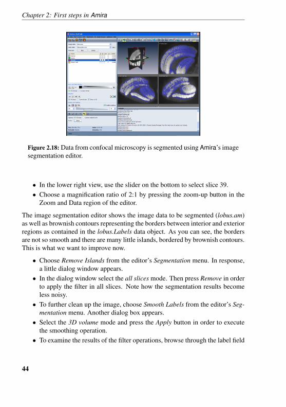
Chapter 2: First steps in Amira
Figure 2.18: Data from confocal microscopy is segmented using Amira’s imagesegmentation editor.
• In the lower right view, use the slider on the bottom to select slice 39.• Choose a magnification ratio of 2:1 by pressing the zoom-up button in the
Zoom and Data region of the editor.
The image segmentation editor shows the image data to be segmented (lobus.am)as well as brownish contours representing the borders between interior and exteriorregions as contained in the lobus.Labels data object. As you can see, the bordersare not so smooth and there are many little islands, bordered by brownish contours.This is what we want to improve now.
• Choose Remove Islands from the editor’s Segmentation menu. In response,a little dialog window appears.
• In the dialog window select the all slices mode. Then press Remove in orderto apply the filter in all slices. Note how the segmentation results becomeless noisy.
• To further clean up the image, choose Smooth Labels from the editor’s Seg-mentation menu. Another dialog box appears.
• Select the 3D volume mode and press the Apply button in order to executethe smoothing operation.
• To examine the results of the filter operations, browse through the label field
44
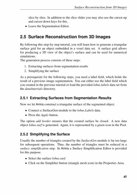
Surface Reconstruction from 3D Images
slice by slice. In addition to the slice slider you may also use the cursor-upand cursor-down keys for this.
• Leave the Segmentation Editor.
2.5 Surface Reconstruction from 3D Images
By following this step-by-step tutorial, you will learn how to generate a triangularsurface grid for an object embedded in a voxel data set. A surface grid allowsfor producing a 3D view of the object’s surface and can be used for numericalsimulations.The generation process consists of these steps:
1. Extracting surfaces from segmentation results2. Simplifying the surface
As a prerequisite for the following steps, you need a label field, which holds theresult of a previous image segmentation. You can either use the label field whichyou created in the previous tutorial or load the provided lobus.labels data set fromthe data/tutorials directory.
2.5.1 Extracting Surfaces from Segmentation Results
Now we let Amira construct a triangular surface of the segmented object.
• Connect a SurfaceGen module to the lobus.Labels data.• Press the Apply button.
The option add border ensures that the created surface be closed. A new dataobject lobus.surf is generated. Again, it is represented by a green icon in the Pool.
2.5.2 Simplifying the Surface
Usually the number of triangles created by the SurfaceGen module is far too largefor subsequent operations. Thus, the number of triangles must be reduced in asurface simplification step. In Amira a Surface Simplification Editor is providedfor this purpose.
• Select the surface lobus.surf.• Click on the Simplifier button (triangle mesh icon) in the Properties Area.
45
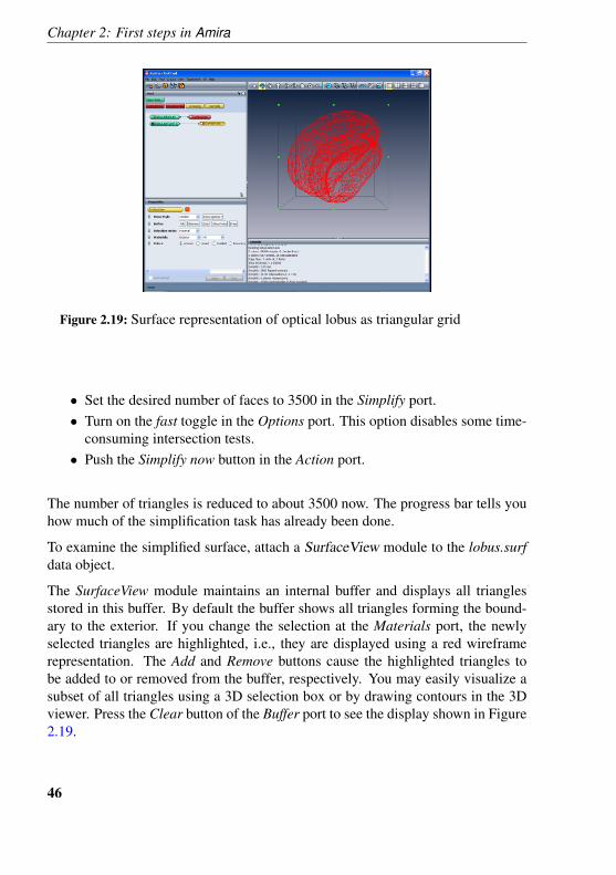
Chapter 2: First steps in Amira
Figure 2.19: Surface representation of optical lobus as triangular grid
• Set the desired number of faces to 3500 in the Simplify port.• Turn on the fast toggle in the Options port. This option disables some time-
consuming intersection tests.• Push the Simplify now button in the Action port.
The number of triangles is reduced to about 3500 now. The progress bar tells youhow much of the simplification task has already been done.
To examine the simplified surface, attach a SurfaceView module to the lobus.surfdata object.
The SurfaceView module maintains an internal buffer and displays all trianglesstored in this buffer. By default the buffer shows all triangles forming the bound-ary to the exterior. If you change the selection at the Materials port, the newlyselected triangles are highlighted, i.e., they are displayed using a red wireframerepresentation. The Add and Remove buttons cause the highlighted triangles tobe added to or removed from the buffer, respectively. You may easily visualize asubset of all triangles using a 3D selection box or by drawing contours in the 3Dviewer. Press the Clear button of the Buffer port to see the display shown in Figure2.19.
46
Creating a Tetrahedral Grid from a Triangular Surface
2.6 Creating a Tetrahedral Grid from a TriangularSurface
By following this step-by-step tutorial, you will learn how to generate a volumetrictetrahedral grid from a triangular surface as created in the previous tutorial. Atetrahedral grid is the basis for producing various views of inner parts of the object,e.g., cuts through it, and is frequently used for numerical simulations.The generation process consists of these steps:
1. Simplifying the surface2. Editing the surface3. Generating a tetrahedral grid
As a prerequisite for the following steps, you need a triangular surface, which isusually the result of a previous surface reconstruction. Load the supplied lobus.surfdata set from the data/tutorials directory.
2.6.1 Simplifying the Surface
Usually the number of triangles created by the SurfaceGen module is far too largefor subsequent operations, e.g., for a numerical simulation. Thus, the number oftriangles should be reduced in a surface simplification step. In Amira a SurfaceSimplification Editor is provided for this purpose. There may be different goalsfor the simplification:
• In computer graphics, one wants to prescribe just the number of faces, be-cause this determines the rendering speed.
• For a numerical simulation, one often wants to specify the maximum edgelength occurring in the grid model.
This tutorial shows how the maximum edge length can be controlled during sim-plification.
• Select the surface lobus.surf.• Click on the Simplifier (triangle mesh icon) in the Properties Area.• Set the desired number of faces to 1000 and the desired maximal distance
(i.e. edge length) to 10 in the Simplify port.• Leave the fast toggle turned off in the Options port. This will cause inter-
section tests to be performed during simplification, which will considerably
47
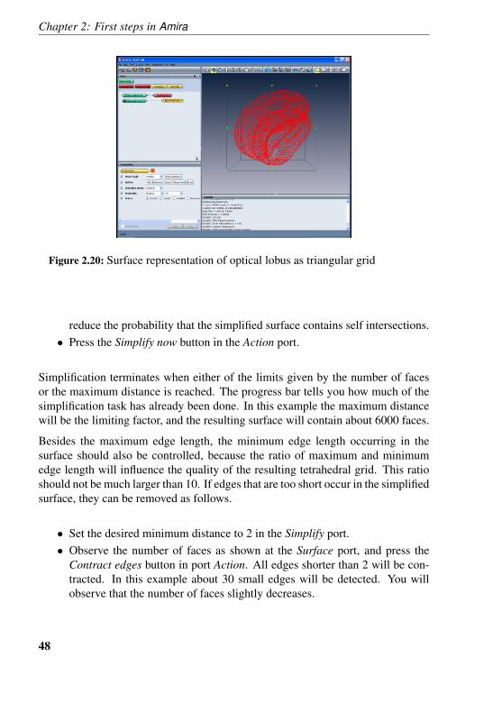
Chapter 2: First steps in Amira
Figure 2.20: Surface representation of optical lobus as triangular grid
reduce the probability that the simplified surface contains self intersections.• Press the Simplify now button in the Action port.
Simplification terminates when either of the limits given by the number of facesor the maximum distance is reached. The progress bar tells you how much of thesimplification task has already been done. In this example the maximum distancewill be the limiting factor, and the resulting surface will contain about 6000 faces.
Besides the maximum edge length, the minimum edge length occurring in thesurface should also be controlled, because the ratio of maximum and minimumedge length will influence the quality of the resulting tetrahedral grid. This ratioshould not be much larger than 10. If edges that are too short occur in the simplifiedsurface, they can be removed as follows.
• Set the desired minimum distance to 2 in the Simplify port.• Observe the number of faces as shown at the Surface port, and press the
Contract edges button in port Action. All edges shorter than 2 will be con-tracted. In this example about 30 small edges will be detected. You willobserve that the number of faces slightly decreases.
48
Creating a Tetrahedral Grid from a Triangular Surface
2.6.2 Editing the Surface
As a second step of preparation for tetrahedral grid generation, invoke the SurfaceEditor.
• Select the surface lobus.surf.• Leave the Surface Simplification Editor (Simplifier) by again clicking on the
triangle mesh icon.• Enter the Surface Editor by clicking on the Surface Editor button in the
Properties Area.
Automatically, a SurfaceView module will be attached to the lobus.surf surface.For details about that module see its description.When the Surface Editor is invoked, the Surface menu is added to Amira’s menubar and a new toolbar is placed just below Amira’s viewer toolbar. The Sur-face/Tests menu contains 6 specific tests which are useful for preparing a tetra-hedral grid generation. Each of the tests creates a buffer of triangles which can becycled through using the back and forward buttons.
• Select Intersection test from the Surface/Tests menu. The total number of in-tersecting triangles is printed in the console window. Intersections shouldn’toccur too often if toggle fast was switched off during surface simplification.In case they occur, the first of the intersecting triangles and its neighbors areshown in the viewer window.
• You can manually repair intersections using four basic operations: EdgeFlip, Edge Collapse, Edge Bisection, and Vertex Translation. See the de-scription of the Surface Editor for details.
• After repairing, invoke the intersection test again by selecting it from theSurface/Tests menu or by pressing the Compute button.
• When the intersection test has been successfully passed, select the Orien-tation test from the Surface/Tests menu. After surface simplification, theorientation of a small number of triangles may be inconsistent, resulting ina partial overlap of the materials bounded by the triangles. In case of suchincorrect orientations, which should occur quite rarely, there is an automaticrepair. If this fails, the detected triangles will be shown, and you can use theabove mentioned manual operations for repair. Note: There are two prereq-uisites for the orientation test: the surface must be free of intersections, andthe outer triangles of the surface must be assigned to material Exterior. Ifthe surface does not contain such a material or if the assignment to Exterior
49
Chapter 2: First steps in Amira
is not correct, the test will falsely report orientation errors.
A successful pass of the intersection and orientation test is mandatory for tetrahe-dral grid generation. These tests are automatically performed at the beginning ofgrid generation. So you can directly enter the TetraGen module (see below) andtry to create a grid. If one of the tests fails, an error message will be issued in theconsole window. You can then go back to the Surface Editor and start editing.The remaining three tests analyze the surface mesh with respect to different qualitymeasures. These tests only need to be performed if the tetrahedral quality of thevolumetric grid plays an important role, e.g., if the grid will be used for a numericalsimulation.
• Select Aspect ratio from the Surface/Tests menu. This computes the ratio ofthe radii of the circumcircle and the incircle for each triangle. The trianglewith the worst (i.e. largest) value is shown first, and the actual value isprinted in the console window. The largest aspect ratio should be below 20(better below 10). Fortunately there is an automatic tool for improving theaspect ratio included in the Surface Editor.
• Select Flip edges from the Edit menu. A small dialog window appears. Inthe Radius Ratio area, set the value of the ”Try to flip a triangle...” field to10. Select mode operate on whole surface. Press button Flip. All triangleswith an aspect ratio larger than 10 will be inspected; if the aspect ratio canbe improved via an edge flip, this will be done automatically. The consolewindow will tell you the total number of bad triangles and how many ofthem could be repaired. Press the Close button to leave the Flip edges tool.
• Select again Aspect ratio from the Surface/Tests menu. Only a small numberof triangles with large aspect ratio should remain after applying the Flipedges tool.
• Select Dihedral angle from the Surface/Tests menu. For each pair of adja-cent triangles, the angle between them at their common edge will be com-puted. The triangle pair including the worst (i.e. smallest) angle is shownin the viewer, and the actual value is printed in the console window. Thesmallest dihedral angle should be larger than 5 degrees (better larger than10).
• For a manual repair of a small dihedral angle proceed as follows: select thethird points of both triangles (i.e. the points opposite to the common edge)and move them away from each other. For moving vertices you must enterVertex Translation mode by clicking on the first icon from the right on the
50
Creating a Tetrahedral Grid from a Triangular Surface
top of the viewer window or by pressing the "t" key. If the viewer is inviewing mode, switch it into interaction mode by pressing the ESC key orby clicking on the arrow icon (the first icon from the top) on the right of theviewer window. Click on the vertex to be moved. At the picked vertex apoint dragger will be shown. Pick and translate the dragger for moving thevertex.
• In some cases an edge flip might also improve the situation. Enter Edge Flipmode by clicking on the third icon from the right on the top of the viewerwindow or by pressing the "f" key. Switch the viewer into interactionmode. Click on the edge to be flipped.
• Select Tetra quality from the Surface/Tests menu. For each surface trianglethe aspect ratio of the tetrahedron which would probably be created for thattriangle will be calculated. The aspect ratio for a tetrahedron is defined asthe ratio of the radii of the circumsphere and the inscribed sphere. Thetriangle with the worst (i.e. largest) value is shown in the viewer, and theactual value is printed in the console window. The largest tetrahedral aspectratio should be below 50 (better below 25). If all small dihedral angles havealready been repaired, the tetra quality test will mainly detect configurationswhere the normal distance between two triangles is small compared to theiredge lengths. Again, the vertex translation and the edge flip operation arebest suited for a manual repair of large tetrahedron aspect ratios.
• Leave the Surface Editor by again clicking on the Surface Editor button inthe Properties Area.
Hint: In order to see the entire surface again, select the SurfaceView icon, thenpress its Show/Hide button, then press the ViewAll button in the viewer toolbar.
2.6.3 Generation of a Tetrahedral Grid
The last step is the generation of a volumetric tetrahedral grid from the surface.This means that the volume enclosed by the surface is filled with tetrahedra.Because the computation of the tetrahedral grid may be time consuming it can beperformed as a batch job. You can then continue working with Amira while thejob is running. However, for demonstration purposes we want to compute the gridright inside Amira.
• Connect a TetraGen module to the lobus.surf surface by choosing ComputeTetraGen from the popup menu over the lobus.surf icon.
51
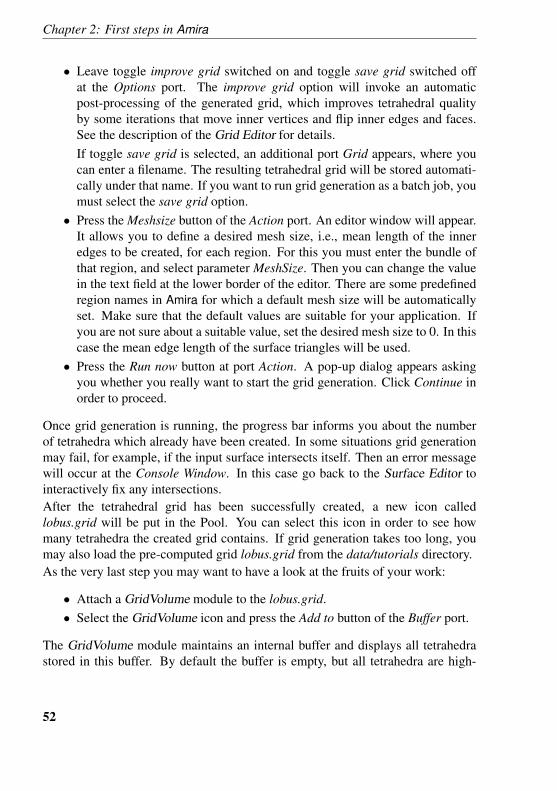
Chapter 2: First steps in Amira
• Leave toggle improve grid switched on and toggle save grid switched offat the Options port. The improve grid option will invoke an automaticpost-processing of the generated grid, which improves tetrahedral qualityby some iterations that move inner vertices and flip inner edges and faces.See the description of the Grid Editor for details.If toggle save grid is selected, an additional port Grid appears, where youcan enter a filename. The resulting tetrahedral grid will be stored automati-cally under that name. If you want to run grid generation as a batch job, youmust select the save grid option.
• Press the Meshsize button of the Action port. An editor window will appear.It allows you to define a desired mesh size, i.e., mean length of the inneredges to be created, for each region. For this you must enter the bundle ofthat region, and select parameter MeshSize. Then you can change the valuein the text field at the lower border of the editor. There are some predefinedregion names in Amira for which a default mesh size will be automaticallyset. Make sure that the default values are suitable for your application. Ifyou are not sure about a suitable value, set the desired mesh size to 0. In thiscase the mean edge length of the surface triangles will be used.
• Press the Run now button at port Action. A pop-up dialog appears askingyou whether you really want to start the grid generation. Click Continue inorder to proceed.
Once grid generation is running, the progress bar informs you about the numberof tetrahedra which already have been created. In some situations grid generationmay fail, for example, if the input surface intersects itself. Then an error messagewill occur at the Console Window. In this case go back to the Surface Editor tointeractively fix any intersections.After the tetrahedral grid has been successfully created, a new icon calledlobus.grid will be put in the Pool. You can select this icon in order to see howmany tetrahedra the created grid contains. If grid generation takes too long, youmay also load the pre-computed grid lobus.grid from the data/tutorials directory.As the very last step you may want to have a look at the fruits of your work:
• Attach a GridVolume module to the lobus.grid.• Select the GridVolume icon and press the Add to button of the Buffer port.
The GridVolume module maintains an internal buffer and displays all tetrahedrastored in this buffer. By default the buffer is empty, but all tetrahedra are high-
52
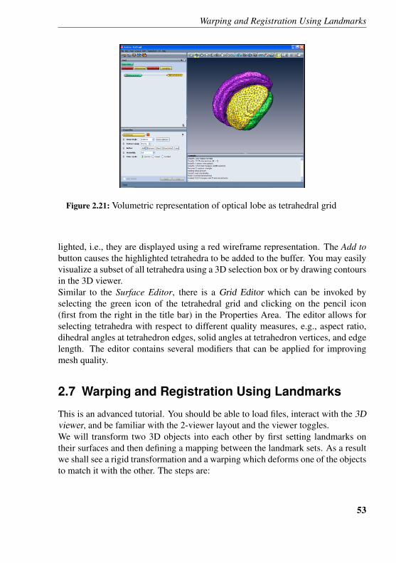
Warping and Registration Using Landmarks
Figure 2.21: Volumetric representation of optical lobe as tetrahedral grid
lighted, i.e., they are displayed using a red wireframe representation. The Add tobutton causes the highlighted tetrahedra to be added to the buffer. You may easilyvisualize a subset of all tetrahedra using a 3D selection box or by drawing contoursin the 3D viewer.Similar to the Surface Editor, there is a Grid Editor which can be invoked byselecting the green icon of the tetrahedral grid and clicking on the pencil icon(first from the right in the title bar) in the Properties Area. The editor allows forselecting tetrahedra with respect to different quality measures, e.g., aspect ratio,dihedral angles at tetrahedron edges, solid angles at tetrahedron vertices, and edgelength. The editor contains several modifiers that can be applied for improvingmesh quality.
2.7 Warping and Registration Using Landmarks
This is an advanced tutorial. You should be able to load files, interact with the 3Dviewer, and be familiar with the 2-viewer layout and the viewer toggles.We will transform two 3D objects into each other by first setting landmarks ontheir surfaces and then defining a mapping between the landmark sets. As a resultwe shall see a rigid transformation and a warping which deforms one of the objectsto match it with the other. The steps are:
53
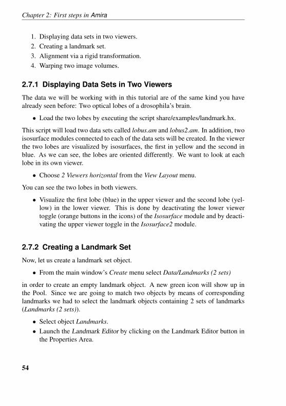
Chapter 2: First steps in Amira
1. Displaying data sets in two viewers.2. Creating a landmark set.3. Alignment via a rigid transformation.4. Warping two image volumes.
2.7.1 Displaying Data Sets in Two Viewers
The data we will be working with in this tutorial are of the same kind you havealready seen before: Two optical lobes of a drosophila’s brain.
• Load the two lobes by executing the script share/examples/landmark.hx.
This script will load two data sets called lobus.am and lobus2.am. In addition, twoisosurface modules connected to each of the data sets will be created. In the viewerthe two lobes are visualized by isosurfaces, the first in yellow and the second inblue. As we can see, the lobes are oriented differently. We want to look at eachlobe in its own viewer.
• Choose 2 Viewers horizontal from the View Layout menu.
You can see the two lobes in both viewers.
• Visualize the first lobe (blue) in the upper viewer and the second lobe (yel-low) in the lower viewer. This is done by deactivating the lower viewertoggle (orange buttons in the icons) of the Isosurface module and by deacti-vating the upper viewer toggle in the Isosurface2 module.
2.7.2 Creating a Landmark Set
Now, let us create a landmark set object.
• From the main window’s Create menu select Data/Landmarks (2 sets)
in order to create an empty landmark object. A new green icon will show up inthe Pool. Since we are going to match two objects by means of correspondinglandmarks we had to select the landmark objects containing 2 sets of landmarks(Landmarks (2 sets)).
• Select object Landmarks.• Launch the Landmark Editor by clicking on the Landmark Editor button in
the Properties Area.
54
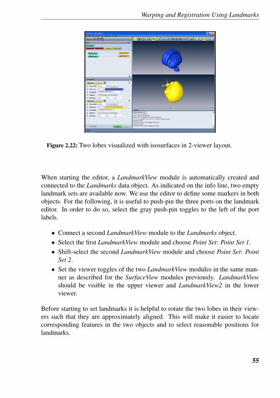
Warping and Registration Using Landmarks
Figure 2.22: Two lobes visualized with isosurfaces in 2-viewer layout.
When starting the editor, a LandmarkView module is automatically created andconnected to the Landmarks data object. As indicated on the info line, two emptylandmark sets are available now. We use the editor to define some markers in bothobjects. For the following, it is useful to push-pin the three ports on the landmarkeditor. In order to do so, select the gray push-pin toggles to the left of the portlabels.
• Connect a second LandmarkView module to the Landmarks object.• Select the first LandmarkView module and choose Point Set: Point Set 1.• Shift-select the second LandmarkView module and choose Point Set: Point
Set 2.• Set the viewer toggles of the two LandmarkView modules in the same man-
ner as described for the SurfaceView modules previously. LandmarkViewshould be visible in the upper viewer and LandmarkView2 in the lowerviewer.
Before starting to set landmarks it is helpful to rotate the two lobes in their view-ers such that they are approximately aligned. This will make it easier to locatecorresponding features in the two objects and to select reasonable positions forlandmarks.
55
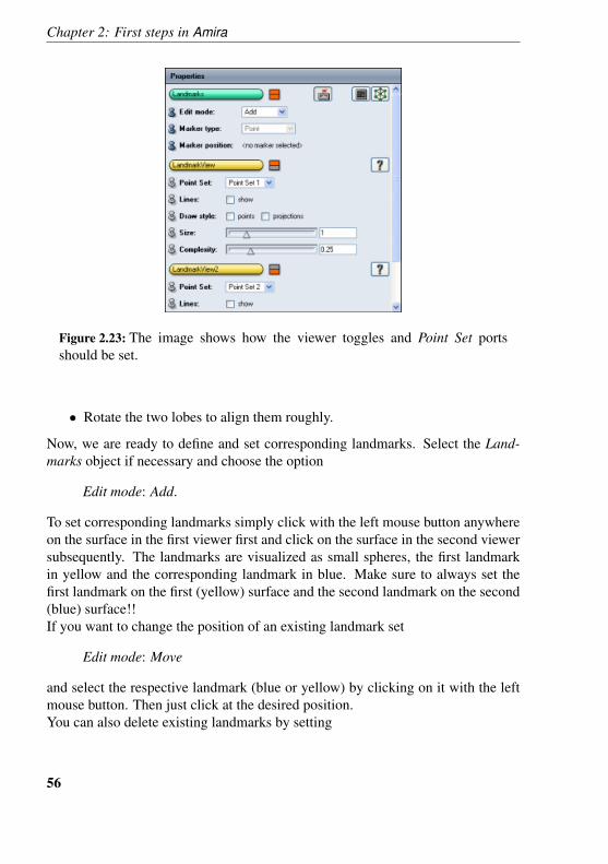
Chapter 2: First steps in Amira
Figure 2.23: The image shows how the viewer toggles and Point Set portsshould be set.
• Rotate the two lobes to align them roughly.
Now, we are ready to define and set corresponding landmarks. Select the Land-marks object if necessary and choose the option
Edit mode: Add.
To set corresponding landmarks simply click with the left mouse button anywhereon the surface in the first viewer first and click on the surface in the second viewersubsequently. The landmarks are visualized as small spheres, the first landmarkin yellow and the corresponding landmark in blue. Make sure to always set thefirst landmark on the first (yellow) surface and the second landmark on the second(blue) surface!!If you want to change the position of an existing landmark set
Edit mode: Move
and select the respective landmark (blue or yellow) by clicking on it with the leftmouse button. Then just click at the desired position.You can also delete existing landmarks by setting
56
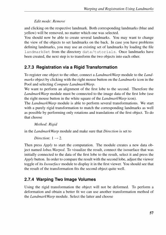
Warping and Registration Using Landmarks
Edit mode: Remove
and clicking on the respective landmark. Both corresponding landmarks (blue andyellow) will be removed, no matter which one was selected.You should now be able to create several landmarks. You may want to changethe view of the objects to set landmarks on the back. In case you have problemsdefining landmarks, you may use an existing set of landmarks by loading the filelandmarkSet from the directory data/tutorials. Once landmarks havebeen created, the next step is to transform the two objects into each other.
2.7.3 Registration via a Rigid Transformation
To register one object to the other, connect a LandmarkWarp module to the Land-marks object by clicking with the right mouse button on the Landmarks icon in thePool and selecting Compute LandmarkWarp.We want to perform an alignment of the first lobe to the second. Therefore theLandmarkWarp module must be connected to the image data of the first lobe (usethe right mouse button in the white square of the LandmarkWarp icon).The LandmarkWarp module is able to perform several transformations. We startwith a purely rigid transformation to match the corresponding landmarks as wellas possible by performing only rotations and translations of the first object. To dothat choose
Method: Rigid
in the LandmarkWarp module and make sure that Direction is set to
Direction: 1→ 2.
Then press Apply to start the computation. The module creates a new data ob-ject named lobus.Warped. To visualize the result, connect the isosurface that wasinitially connected to the data of the first lobe to the result, select it and press theApply button. In order to compare the result with the second lobe, adjust the viewertoggle of its Isosurface module to display it in the first viewer. You should see thatthe result of the transformation fits the second object quite well.
2.7.4 Warping Two Image Volumes
Using the rigid transformation the object will not be deformed. To perform adeformation and obtain a better fit we can use another transformation method ofthe LandmarkWarp module. Select the latter and choose
57
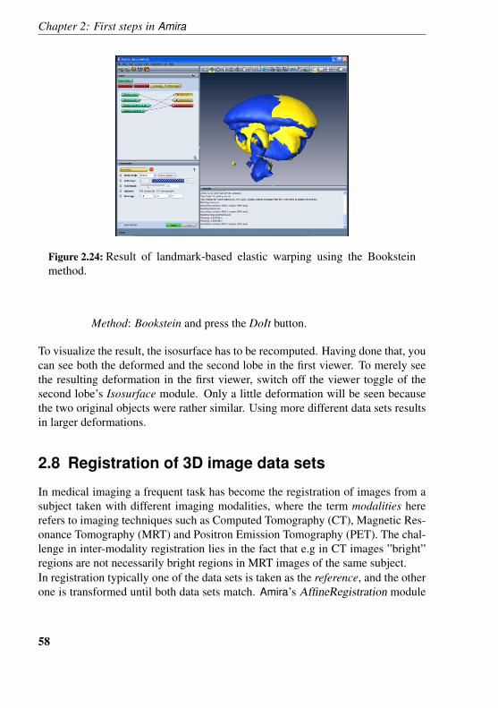
Chapter 2: First steps in Amira
Figure 2.24: Result of landmark-based elastic warping using the Booksteinmethod.
Method: Bookstein and press the DoIt button.
To visualize the result, the isosurface has to be recomputed. Having done that, youcan see both the deformed and the second lobe in the first viewer. To merely seethe resulting deformation in the first viewer, switch off the viewer toggle of thesecond lobe’s Isosurface module. Only a little deformation will be seen becausethe two original objects were rather similar. Using more different data sets resultsin larger deformations.
2.8 Registration of 3D image data sets
In medical imaging a frequent task has become the registration of images from asubject taken with different imaging modalities, where the term modalities hererefers to imaging techniques such as Computed Tomography (CT), Magnetic Res-onance Tomography (MRT) and Positron Emission Tomography (PET). The chal-lenge in inter-modality registration lies in the fact that e.g in CT images ”bright”regions are not necessarily bright regions in MRT images of the same subject.In registration typically one of the data sets is taken as the reference, and the otherone is transformed until both data sets match. Amira’s AffineRegistration module
58
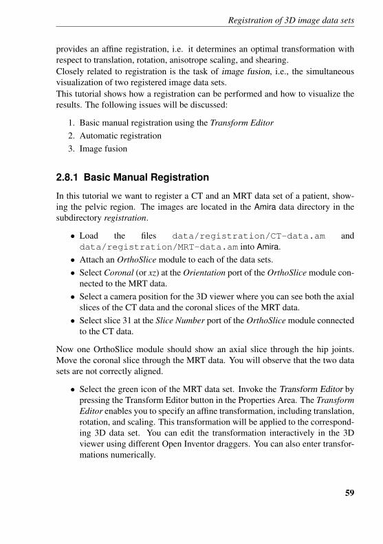
Registration of 3D image data sets
provides an affine registration, i.e. it determines an optimal transformation withrespect to translation, rotation, anisotrope scaling, and shearing.Closely related to registration is the task of image fusion, i.e., the simultaneousvisualization of two registered image data sets.This tutorial shows how a registration can be performed and how to visualize theresults. The following issues will be discussed:
1. Basic manual registration using the Transform Editor2. Automatic registration3. Image fusion
2.8.1 Basic Manual Registration
In this tutorial we want to register a CT and an MRT data set of a patient, show-ing the pelvic region. The images are located in the Amira data directory in thesubdirectory registration.
• Load the files data/registration/CT-data.am anddata/registration/MRT-data.am into Amira.
• Attach an OrthoSlice module to each of the data sets.• Select Coronal (or xz) at the Orientation port of the OrthoSlice module con-
nected to the MRT data.• Select a camera position for the 3D viewer where you can see both the axial
slices of the CT data and the coronal slices of the MRT data.• Select slice 31 at the Slice Number port of the OrthoSlice module connected
to the CT data.
Now one OrthoSlice module should show an axial slice through the hip joints.Move the coronal slice through the MRT data. You will observe that the two datasets are not correctly aligned.
• Select the green icon of the MRT data set. Invoke the Transform Editor bypressing the Transform Editor button in the Properties Area. The TransformEditor enables you to specify an affine transformation, including translation,rotation, and scaling. This transformation will be applied to the correspond-ing 3D data set. You can edit the transformation interactively in the 3Dviewer using different Open Inventor draggers. You can also enter transfor-mations numerically.
59
Chapter 2: First steps in Amira
• Press the Dialog button. A dialog window will pop up.• Enter -2 at the third text field of the Translation port of the dialog window.
This means a translation of -2 cm in the z direction.• Enter 5 at the first text field at the Rotation port. This means a rotation of 5
degrees. The axis of rotation is defined at the next ports, here it is the z-axis.• Press the Close button of the dialog window. Leave the Transform Editor by
pressing again the Transform Editor button.
Inspect some coronal slices through the MRT data set. Now there is a better align-ment of the CT and MRT data, but it’s still not perfect.
2.8.2 Automatic Registration
The Registration module provides an automatic registration via optimization of aquality function. For registration of data sets from different imaging modalities,the Normalized Mutual Information is the best suited quality function. In short,it favors an alignment which ”maps similar gray value structures to similar grayvalue structures”. A hierarchical strategy is applied, starting at a coarse resamplingof the data sets, and proceeding to finer resolutions later on.
• Attach an Registration module to the MRT data set by choosing Com-pute/AffineRegistration from the popup menu over the MRT-data.am icon.
• Connect the second input port Reference of module Registration to the CTdata set. For this click with the right mouse button on the white square atthe left hand side of the module’s icon.
• Select toggle Extended options. More ports of the Registration module willbecome visible.
The first three ports of the Registration module define the optimization strategy.The default settings mean that an ExtensiveDirection optimizer is used for thecoarse levels and a QuasiNewton optimizer for the finest two levels of the resam-pling hierarchy. At the CoarsestResampling port you can select the resamplingrate for the coarsest resolution level. The default resampling rate is smaller in thez direction because the reference data set has a finer resolution in the x and y di-rection (0.17 cm) than in the z direction (0.5 cm). For the default settings (8,8,3),the resampling hierarchy will consist of four levels: (8,8,3), (4,4,2), (2,2,1), andthe original resolution, (1,1,1).
60
Registration of 3D image data sets
The Normalized Mutual Information is calculated from gray value histograms. Theselected histogram ranges should enclose the essential information of each data set.Normally you can choose the same range as for visualization via an OrthoSlicemodule.
• Set -200 and 200 at the two text fields of the Histogram range referenceport.
At the Transform port you can specify the type of affine transformation. The de-fault settings mean that only rigid body motions will be applied, i.e. translationsand rotations.Option Ignore finest resolution means that optimization is done on all but the finestlevel of the resampling hierarchy. This will slightly reduce the accuracy, but savea large amount of computing time.Automatic registration may take some time depending on the resolution of theimages and the quality of the pre-alignment. You can interrupt automatic registra-tion at any time using the stop button. Interruption may take some seconds. Theprogress bar shows the current hierarchy level and the progress at that level.
• Start automatic registration by pressing the Register button at the Actionport.
2.8.3 Image Fusion
The task of image fusion is the simultaneous visualization of two data sets. To thatend Amira offers for all types of slicing modules (Orthoslice and ObliqueSlice)the Colorwash module. Using Colorwash, the images from one data set can beoverlayed over that of another taking into account their orientation in space.
• Remove the OrthoSlice module connected to the MRT data set.• Select the green icon of the MRT data set.• Select a Colorwash module from the popup menu over the icon of the Or-
thoSlice module connected to the CT data set.• Select the yellow icon of the Colorwash module.• Select the physics.icol colormap at port Colormap.• Set 70 as the upper bound for the colormap range.• Select the icon of the OrthoSlice module.• Inspect axial slices with slice numbers between 15 and 45.
61
Chapter 2: First steps in Amira
You will observe a good alignment of the pelvic bone from both data sets. The softtissue contours are not perfectly aligned because there was some soft tissue defor-mation between both scans. This cannot be described by a rigid transformation.In image fusion it is sometimes necessary to observe all three orthogonal directionssimultaneously. For that the StandardView module can be used for image fusion.The StandardView module opens a separate window with four viewers, three ofthem showing the three orthogonal slices of the image data and a fourth being anew instance of the 3D viewer.
• Attach a StandardView module to the CT data set by choosing Display Stan-dardView from the popup menu over the CT-data.am icon. Amira’s Viewerwindow will now be split into four parts showing three orthogonal slicesthrough the CT data, and the 3D Viewer in the upper left part.
• Connect the second input port OverlayData of the StandardView module tothe MRT data set. For this, click with the right mouse button on the whitesquare at the left hand side of the module’s icon.
• Select slice numbers 179, 149, and 31 at ports Slice x, Slice y, and Slice z,respectively. The three orthogonal slices will show the hip joints now.
• Increase the zoom-factor by clicking twice on button > at the Zoom port.• Select checkerboard at the Overlay mode port.• Vary the size of the checkerboard tiles by moving the slider at the Pattern
size port. In this way you can again check the alignment of the CT and MRTdata sets.
The bone contours around the hip joints show a good match. Note that bone isrepresented by white (i.e high intensity) voxels in the CT data, but may occur asboth white and black voxels in the MRT data. In the axial slice you can observelarger deviations of the outer body contour between the CT and MRT data.
2.9 Alignment of 2D Physical Cross-sections
Many microscopic techniques require the sample to be physically cut into slices.Then images are taken from each cross-section separately. Usually the imageswill be misaligned relative to each other. Before a 3-dimensional model of thesample can be reconstructed the images have to be aligned taking into accounttranslation and rotation. This tutorial shows how this task can be performed usingthe AlignSlices module.
62
Alignment of 2D Physical Cross-sections
The following issues will be discussed:
1. Basic manual alignment2. Alignment via landmarks3. Optimizing the quality function4. Resampling the input data5. Other alignment options
2.9.1 Basic Manual Alignment
In this tutorial we want to align 10 microscopic cross-sections of a leaf showinga stomatal pore. The images are located in the data directory in the subdirectoryalign. Each slice is stored as a separate JPEG image. The file leaf.info defines a3D image stack consisting of the 10 individual slices. It is a simple ASCII file asdescribed in the stacked slices file format section.
• Load the file data/align/leaf.info.• Create an align module by choosing Compute AlignSlices from the popup
menu over the leaf.info icon.• Press the Edit button of AlignSlices.
A new graphics window is popped up allowing you to interactively align the slicesof the 3D image stack. To facilitate this task, usually two consecutive slices aredisplayed simultaneously. One of the two slices is editable, i.e., it can be trans-lated and rotated using the mouse. By default the upper slice is editable. This isindicated in the tool bar of the align window (the ”upper slice” button is selected).
• If necessary, press the zoom out button (”-” magnifying glass) to allow theentire slice to be visible in viewer.
• Translate the upper slice by moving the mouse with the left mouse buttonpressed down.
• Rotate the upper slice by moving the mouse with the left mouse button andthe Ctrl key pressed down. Alternatively, slices can be rotated using themiddle mouse button.
• Make the lower slice editable by selecting the ”lower slice” tool button.Translate and rotate the lower slice.
• Hold down key number 1. While this key is hold down only the lower sliceis displayed.
63
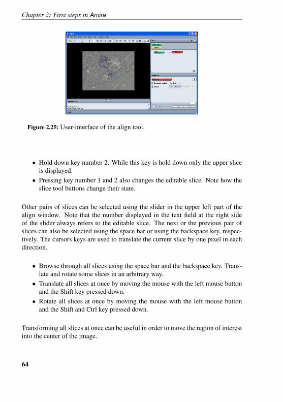
Chapter 2: First steps in Amira
Figure 2.25: User-interface of the align tool.
• Hold down key number 2. While this key is hold down only the upper sliceis displayed.
• Pressing key number 1 and 2 also changes the editable slice. Note how theslice tool buttons change their state.
Other pairs of slices can be selected using the slider in the upper left part of thealign window. Note that the number displayed in the text field at the right sideof the slider always refers to the editable slice. The next or the previous pair ofslices can also be selected using the space bar or using the backspace key, respec-tively. The cursors keys are used to translate the current slice by one pixel in eachdirection.
• Browse through all slices using the space bar and the backspace key. Trans-late and rotate some slices in an arbitrary way.
• Translate all slices at once by moving the mouse with the left mouse buttonand the Shift key pressed down.
• Rotate all slices at once by moving the mouse with the left mouse buttonand the Shift and Ctrl key pressed down.
Transforming all slices at once can be useful in order to move the region of interestinto the center of the image.
64
Alignment of 2D Physical Cross-sections
2.9.2 Alignment Via Landmarks
Besides manual alignment, four automatic alignment options are supported,namely alignment using a principal axes transformation, automatic optimization ofa quality function, edge detection-based alignment and alignment via user-definedlandmarks. The principal axes method and the edge detection method are only suit-able for images showing an object which clearly separates from the background.The optimization method requires that the images be already roughly aligned. Of-ten such a pre-alignment can be achieved using the landmarks method.Alignment via landmarks first requires you to interactively define the positions ofthe landmarks. This can be done in landmark edit mode.
• Activate landmark edit mode by pressing the arrow-shape tool button lo-cated between the hand-shape button and the edge detection button.
In landmark edit mode only one slice is displayed instead of two. Two defaultlandmarks are defined in every slice.
• Click on one of the default landmarks. The landmark gets selected and isdrawn with a red border.
• Click somewhere into the image in order to reposition the selected landmark.• Click somewhere into the image while no landmark is selected. This causes
the next landmark to be selected automatically.• Click at the same position again in order to reposition the next landmark.
The double-click method makes it very easy to define landmark positions. Ofcourse, additional landmarks can be defined as well. Landmarks can also bedeleted, but the minimum number of landmarks is two.
• Choose Add from the Landmarks menu.• Click anywhere into the image in order to define the position of the new
landmark.• Select the yellow landmark by clicking on it.• Choose Remove from the Landmarks menu in order to delete the selected
landmark again.
Two landmarks should be visible now, a red one, and a blue one. Next, let us movethese landmarks to some reasonable positions so that we can perform an alignment.
• Select slice number 0.
65
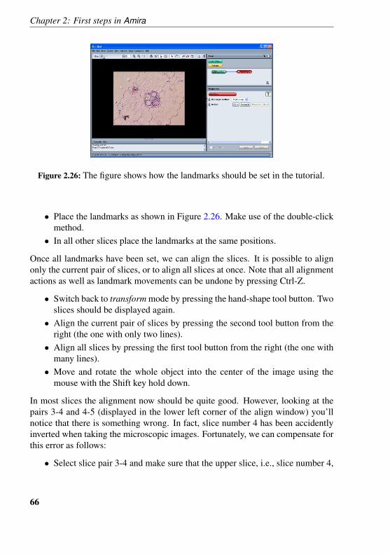
Chapter 2: First steps in Amira
Figure 2.26: The figure shows how the landmarks should be set in the tutorial.
• Place the landmarks as shown in Figure 2.26. Make use of the double-clickmethod.
• In all other slices place the landmarks at the same positions.
Once all landmarks have been set, we can align the slices. It is possible to alignonly the current pair of slices, or to align all slices at once. Note that all alignmentactions as well as landmark movements can be undone by pressing Ctrl-Z.
• Switch back to transform mode by pressing the hand-shape tool button. Twoslices should be displayed again.
• Align the current pair of slices by pressing the second tool button from theright (the one with only two lines).
• Align all slices by pressing the first tool button from the right (the one withmany lines).
• Move and rotate the whole object into the center of the image using themouse with the Shift key hold down.
In most slices the alignment now should be quite good. However, looking at thepairs 3-4 and 4-5 (displayed in the lower left corner of the align window) you’llnotice that there is something wrong. In fact, slice number 4 has been accidentlyinverted when taking the microscopic images. Fortunately, we can compensate forthis error as follows:
• Select slice pair 3-4 and make sure that the upper slice, i.e., slice number 4,
66
Alignment of 2D Physical Cross-sections
is editable.• Invert the upper slice by pressing the invert button (third one from the right).• Realign the current pair of slices by pressing the second button from the
right).• Select slice pair 4-5 and realign this pair of slices as well.
Alternatively, you could have aligned all slices from scratch by pressing the firstbutton from the right.
2.9.3 Optimizing the Quality Function
Once all slices are roughly aligned, we can further improve the alignment using theautomatic optimization method. At the bottom of the align window the quality ofthe current alignment is displayed. This is a number between 0 and 100, where 100indicates a perfect match. The quality function is computed from the squared grayvalue differences of the two slices. The optimization method tries to maximize thequality function. Since only local maxima are found, it is required that the slicesbe reasonably well aligned in advance.
• Click on the slice in the viewer. The quality of the alignment is displayedin the status bar at the bottom of the window. Remember the current qualitymeasure.
• Activate the optimization mode by pressing the tool button with the sum xsquared symbol.
• Align the current pair of slices by pressing the second button from the right.Observe how the quality is improved.
Automatic alignment is an iterative process. It may take quite a long time depend-ing on the resolution of the images and of the quality of the pre-alignment. Youcan interrupt automatic alignment at any time using the Stop button.
• Automatically align all slices by pressing the first button from the right.
2.9.4 Resampling the Input Data
If you are satisfied with the alignment, you can resample the input data set in orderto create a new aligned 3D image. This is done using the Resample button of theAlignSlices module.
67
Chapter 2: First steps in Amira
• Press the Resample button of the AlignSlices module.• Attach an OrthoSlice module to the resulting object leaf.align and verify
that the slices are aligned.
Sometimes you may want to improve an alignment later on. In this case it is a badidea to align the resampled data set a second time, since this would require a secondresampling operation. Instead, you could write the transformation data into theoriginal image object and store this object in AmiraMesh format. After reloadingthe AmiraMesh file you can attach a new AlignSlices module and continue with thestored transformations.
• Choose Save transformation from the Options menu of the align tool. Thiswill store the transformation data in the parameter section of the input objectleaf.info.
• Delete the AlignSlices module.• Save leaf.info in AmiraMesh format.• Reload the saved object leaf.am.• Attach a new AlignSlices module to leaf.am and click the Edit button. Note
that the original alignment is restored.
2.9.5 Using a Reference Image
In some cases you might want to correct the alignment after image segmentationhas been performed. In order to avoid segmenting the newly resampled image fromscratch, you can apply the same transformations to a label field using a referenceimage.
• Delete any existing align tool.• Load the file data/align/leaf-unaligned.labels.• Attach a new AlignSlices module to the label field.
In the label field the guard cells of the stomatal pore are marked. Segmentation hasbeen performed before the images were aligned. Now we want to apply the sametransformation defined for the image data to the labels.
• Connect the Reference port of AlignSlices to leaf.am (this is done by activat-ing the popup menu over the small white square at the left side of the leaf.amicon). Observe how the transformations are applied to the label field.
• Export an aligned label field by pressing the Resample button.
68
Visualization of Vector Fields
The image volume used in this tutorial is an RGBA color field. However, the imagesegmentation editor only supports gray level images. Therefore you must convertthe color field into a scalar field using CastField before you can invoke the imagesegmentation editor for the resampled labels.
2.10 Visualization of Vector Fields
This step-by-step-tutorial briefly explains some Mesh Option modules for vectorfield visualization. The use of these modules is explained by visualizing data rep-resenting the blood flow inside the carotid artery obtained with a simple numericalsimulation. The image data used to segment the carotid are courtesey of Dr. Sell,University of Erlangen, Germany.The following topics will be covered in this tutorial:
1. How to simply represent of a vector field2. Use of Illuminated Stream Lines to visualize the flow3. Extend the visualization with animated Particle Plot
2.10.1 Simple Vector Representation
As in the previous tutorials, we will use the file dialog to import data.
• Load the surface model of the carotids bloodFlow.surf.am from the tutorialdirectory data/tutorials/vector.
• Attach an SurfaceView module to this data object (see the Surface recon-struction tutorial).
• Load the data set called bloodFlow.vector.am from the tutorial direc-tory data/tutorials/vector.
• Connect a Vectors module to the vector field bloodFlow.vector.am.
The vector field itself is stored in Amira’s native AmiraMesh file format. Thedata represents the simulated flow inside the carotids computed on a regular grid.By selecting the green data icon bloodFlow.vector.am, you can find out in theProperties that the number of grid nodes in x,y,z-direction is 116 x 81 x 227.Besides SurfaceView, two new objects are available now in the Pool, Vectors andEmptyPlane. The module Vectors specifies how the vectors are visualized and themodule EmptyPlane identifies on which the plane.
69
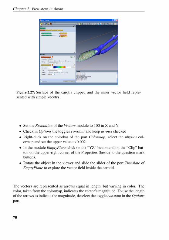
Chapter 2: First steps in Amira
Figure 2.27: Surface of the carotis clipped and the inner vector field repre-sented with simple vecotrs
• Set the Resolution of the Vectors module to 100 in X and Y• Check in Options the toggles constant and keep arrows checked• Right-click on the colorbar of the port Colormap, select the physics col-
ormap and set the upper value to 0.002.• In the module EmptyPlane click on the ”YZ” button and on the ”Clip” but-
ton on the upper-right corner of the Properties (beside to the question markbutton).
• Rotate the object in the viewer and slide the slider of the port Translate ofEmptyPlane to explore the vector field inside the carotid.
The vectors are represented as arrows equal in length, but varying in color. Thecolor, taken from the colormap, indicates the vector’s magnitude. To use the lengthof the arrows to indicate the magnitude, deselect the toggle constant in the Optionsport.
70
Visualization of Vector Fields
2.10.2 Illuminated Stream Lines
Illuminated Stream Lines is a technique for interactive 3D vector field visualizationwhich makes use of large numbers of properly illuminated stream lines. A realisticshading model is employed which significantly increases realism of the resultingimages and enhances spatial perception.Now you will learn which tools are used for illuminated stream line visualizationand how to use them to get a 3D impression of our blood flow vector field.
• Remove the Vectors module.• Connect a DisplayISL module to the vector field bloodFlow.vector.am by
right-clicking on it and selecting Display-¿Vectors.• Set Num Lines to 300.• Press the Apply button.
A TabBox appears in the viewer. Only stream lines flowing through this box arevisible. The green tabs at the corners and edges of the box allow you to change thedimensions of the box.
• Switch the viewer into interact mode.• Try out what happens if you click with the left mouse button on one of the
green tabs on the corners or edges of the TabBox and drag them around.• To move the whole TabBox, click with the left mouse button in the box and
move it.• Try to get the TabBox into a shape and position as shown in the image.• Press Apply button again in order to recalculate the stream lines.• As we did before, slide the slider of the port Translate of EmptyPlane to
explore the vector field inside the carotid.
You can colorize of the stream lines according to a scalar data set of the same sizeand even animate the lines.
• Load bloodFlow.density.am from the tutorial directorydata/tutorials/vector. This data set represents the 3D scalar fieldof the simulated fluid densitiy associated with the 3D vector field.
• Click on the white little square of the DisplayISL icon, select Color Fieldand attach bloodFlow.density.am.
• The port Colormap is now available in the Properties window of DisplayISL.Right-click on the color bar and select temperature.icol, set the colormap
71
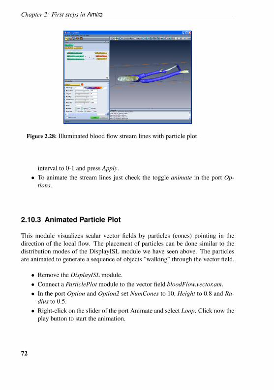
Chapter 2: First steps in Amira
Figure 2.28: Illuminated blood flow stream lines with particle plot
interval to 0-1 and press Apply.• To animate the stream lines just check the toggle animate in the port Op-
tions.
2.10.3 Animated Particle Plot
This module visualizes scalar vector fields by particles (cones) pointing in thedirection of the local flow. The placement of particles can be done similar to thedistribution modes of the DisplayISL module we have seen above. The particlesare animated to generate a sequence of objects ”walking” through the vector field.
• Remove the DisplayISL module.• Connect a ParticlePlot module to the vector field bloodFlow.vector.am.• In the port Option and Option2 set NumCones to 10, Height to 0.8 and Ra-
dius to 0.5.• Right-click on the slider of the port Animate and select Loop. Click now the
play button to start the animation.
72
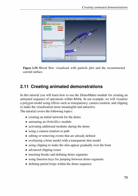
Creating animated demonstrations
Figure 2.29: Blood flow visualized with particle plot and the reconstructedcarotid surface
2.11 Creating animated demonstrations
In this tutorial you will learn how to use the DemoMaker module for creating ananimated sequence of operations within Amira. In our example, we will visualizea polygon model using effects such as transparency, camera rotation, and clippingto make the visualization more meaningful and attractive.The tutorial covers the following topics:
• creating an initial network for the demo• animating an OrthoSlice module• activating additional modules during the demo• using a camera rotation or path• editing or removing events that are already defined• overlaying a bone model with a transparent skin model• using clipping to make the skin appear gradually over the bone• advanced clipping issues• inserting breaks and defining demo segments• using function keys for jumping between demo segments• defining partial loops within the demo sequence
73
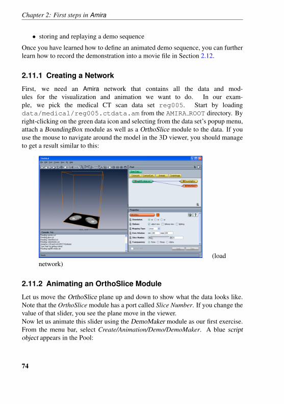
Chapter 2: First steps in Amira
• storing and replaying a demo sequence
Once you have learned how to define an animated demo sequence, you can furtherlearn how to record the demonstration into a movie file in Section 2.12.
2.11.1 Creating a Network
First, we need an Amira network that contains all the data and mod-ules for the visualization and animation we want to do. In our exam-ple, we pick the medical CT scan data set reg005. Start by loadingdata/medical/reg005.ctdata.am from the AMIRA ROOT directory. Byright-clicking on the green data icon and selecting from the data set’s popup menu,attach a BoundingBox module as well as a OrthoSlice module to the data. If youuse the mouse to navigate around the model in the 3D viewer, you should manageto get a result similar to this:
(loadnetwork)
2.11.2 Animating an OrthoSlice Module
Let us move the OrthoSlice plane up and down to show what the data looks like.Note that the OrthoSlice module has a port called Slice Number. If you change thevalue of that slider, you see the plane move in the viewer.Now let us animate this slider using the DemoMaker module as our first exercise.From the menu bar, select Create/Animation/Demo/DemoMaker. A blue scriptobject appears in the Pool:
74
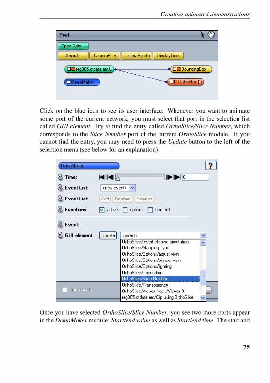
Creating animated demonstrations
Click on the blue icon to see its user interface. Whenever you want to animatesome port of the current network, you must select that port in the selection listcalled GUI element. Try to find the entry called OrthoSlice/Slice Number, whichcorresponds to the Slice Number port of the current OrthoSlice module. If youcannot find the entry, you may need to press the Update button to the left of theselection menu (see below for an explanation).
Once you have selected OrthoSlice/Slice Number, you see two more ports appearin the DemoMaker module: Start/end value as well as Start/end time. The start and
75
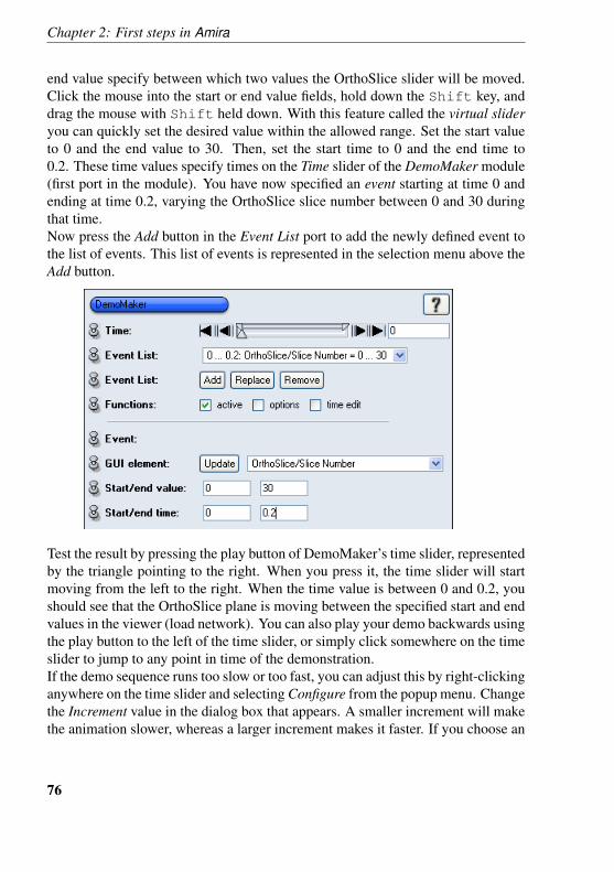
Chapter 2: First steps in Amira
end value specify between which two values the OrthoSlice slider will be moved.Click the mouse into the start or end value fields, hold down the Shift key, anddrag the mouse with Shift held down. With this feature called the virtual slideryou can quickly set the desired value within the allowed range. Set the start valueto 0 and the end value to 30. Then, set the start time to 0 and the end time to0.2. These time values specify times on the Time slider of the DemoMaker module(first port in the module). You have now specified an event starting at time 0 andending at time 0.2, varying the OrthoSlice slice number between 0 and 30 duringthat time.Now press the Add button in the Event List port to add the newly defined event tothe list of events. This list of events is represented in the selection menu above theAdd button.
Test the result by pressing the play button of DemoMaker’s time slider, representedby the triangle pointing to the right. When you press it, the time slider will startmoving from the left to the right. When the time value is between 0 and 0.2, youshould see that the OrthoSlice plane is moving between the specified start and endvalues in the viewer (load network). You can also play your demo backwards usingthe play button to the left of the time slider, or simply click somewhere on the timeslider to jump to any point in time of the demonstration.If the demo sequence runs too slow or too fast, you can adjust this by right-clickinganywhere on the time slider and selecting Configure from the popup menu. Changethe Increment value in the dialog box that appears. A smaller increment will makethe animation slower, whereas a larger increment makes it faster. If you choose an
76
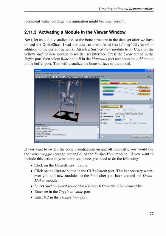
Creating animated demonstrations
increment value too large, the animation might become ”jerky”.
2.11.3 Activating a Module in the Viewer Window
Next, let us add a visualization of the bone structure in the data set after we havemoved the OrthoSlice. Load the data set data/medical/reg005.surf inaddition to the current network. Attach a SurfaceView module to it. Click on theyellow SurfaceView module to see its user interface. Press the Clear button in theBuffer port, then select Bone and All in the Materials port and press the Add buttonin the buffer port. This will visualize the bone surface of the model.
If you want to switch the bone visualization on and off manually, you would usethe viewer toggle (orange rectangle) of the SurfaceView module. If you want toinclude this action in your demo sequence, you need to do the following:
• Click on the DemoMaker module.• Click on the Update button in the GUI element port. This is necessary when-
ever you add new modules to the Pool after you have created the Demo-Maker module.
• Select SurfaceView/Viewer Mask/Viewer 0 from the GUI element list.• Enter on in the Toggle to value port.• Enter 0.2 in the Trigger time port.
77
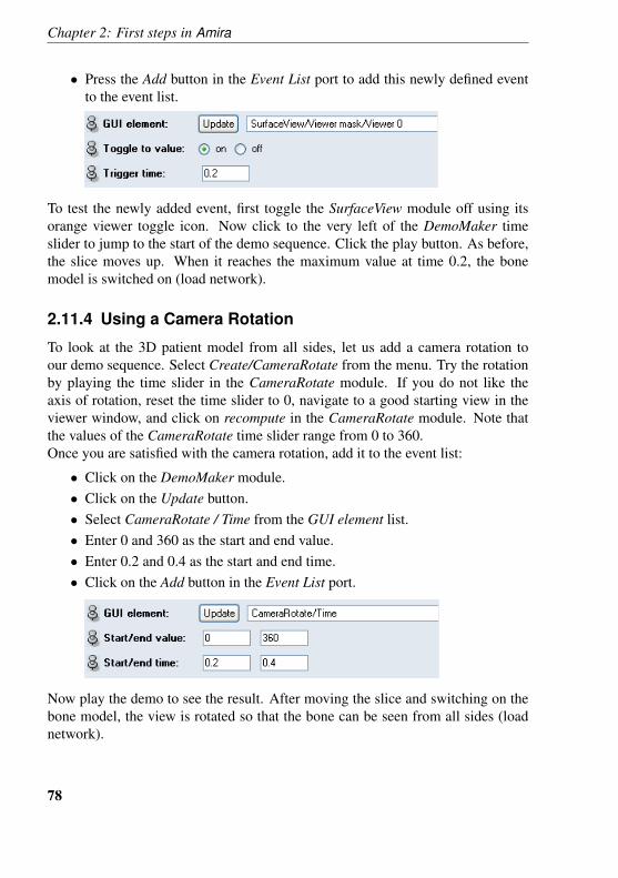
Chapter 2: First steps in Amira
• Press the Add button in the Event List port to add this newly defined eventto the event list.
To test the newly added event, first toggle the SurfaceView module off using itsorange viewer toggle icon. Now click to the very left of the DemoMaker timeslider to jump to the start of the demo sequence. Click the play button. As before,the slice moves up. When it reaches the maximum value at time 0.2, the bonemodel is switched on (load network).
2.11.4 Using a Camera Rotation
To look at the 3D patient model from all sides, let us add a camera rotation toour demo sequence. Select Create/CameraRotate from the menu. Try the rotationby playing the time slider in the CameraRotate module. If you do not like theaxis of rotation, reset the time slider to 0, navigate to a good starting view in theviewer window, and click on recompute in the CameraRotate module. Note thatthe values of the CameraRotate time slider range from 0 to 360.Once you are satisfied with the camera rotation, add it to the event list:
• Click on the DemoMaker module.• Click on the Update button.• Select CameraRotate / Time from the GUI element list.• Enter 0 and 360 as the start and end value.• Enter 0.2 and 0.4 as the start and end time.• Click on the Add button in the Event List port.
Now play the demo to see the result. After moving the slice and switching on thebone model, the view is rotated so that the bone can be seen from all sides (loadnetwork).
78
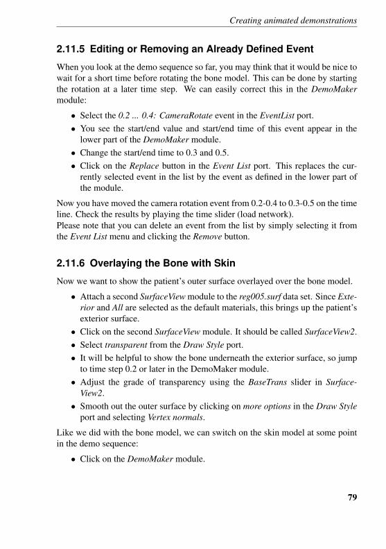
Creating animated demonstrations
2.11.5 Editing or Removing an Already Defined Event
When you look at the demo sequence so far, you may think that it would be nice towait for a short time before rotating the bone model. This can be done by startingthe rotation at a later time step. We can easily correct this in the DemoMakermodule:
• Select the 0.2 ... 0.4: CameraRotate event in the EventList port.• You see the start/end value and start/end time of this event appear in the
lower part of the DemoMaker module.• Change the start/end time to 0.3 and 0.5.• Click on the Replace button in the Event List port. This replaces the cur-
rently selected event in the list by the event as defined in the lower part ofthe module.
Now you have moved the camera rotation event from 0.2-0.4 to 0.3-0.5 on the timeline. Check the results by playing the time slider (load network).Please note that you can delete an event from the list by simply selecting it fromthe Event List menu and clicking the Remove button.
2.11.6 Overlaying the Bone with Skin
Now we want to show the patient’s outer surface overlayed over the bone model.
• Attach a second SurfaceView module to the reg005.surf data set. Since Exte-rior and All are selected as the default materials, this brings up the patient’sexterior surface.
• Click on the second SurfaceView module. It should be called SurfaceView2.• Select transparent from the Draw Style port.• It will be helpful to show the bone underneath the exterior surface, so jump
to time step 0.2 or later in the DemoMaker module.• Adjust the grade of transparency using the BaseTrans slider in Surface-
View2.• Smooth out the outer surface by clicking on more options in the Draw Style
port and selecting Vertex normals.
Like we did with the bone model, we can switch on the skin model at some pointin the demo sequence:
• Click on the DemoMaker module.
79
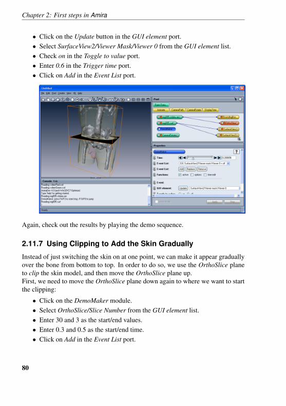
Chapter 2: First steps in Amira
• Click on the Update button in the GUI element port.• Select SurfaceView2/Viewer Mask/Viewer 0 from the GUI element list.• Check on in the Toggle to value port.• Enter 0.6 in the Trigger time port.• Click on Add in the Event List port.
Again, check out the results by playing the demo sequence.
2.11.7 Using Clipping to Add the Skin Gradually
Instead of just switching the skin on at one point, we can make it appear graduallyover the bone from bottom to top. In order to do so, we use the OrthoSlice planeto clip the skin model, and then move the OrthoSlice plane up.First, we need to move the OrthoSlice plane down again to where we want to startthe clipping:
• Click on the DemoMaker module.• Select OrthoSlice/Slice Number from the GUI element list.• Enter 30 and 3 as the start/end values.• Enter 0.3 and 0.5 as the start/end time.• Click on Add in the Event List port.
80
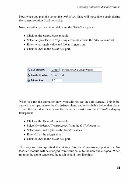
Creating animated demonstrations
Now, when you play the demo, the OrthoSlice plane will move down again duringthe camera rotation (load network).
Now, we will clip the skin model using the OrthoSlice plane:
• Click on the DemoMaker module.• Select SurfaceView2 / Clip using OrthoSlice from the GUI element list.• Enter on as toggle value and 0.6 as trigger time.• Click on Add in the Event List port.
When you run the animation now, you will not see the skin surface. This is be-cause it is clipped above the OrthoSlice plane, and only visible below that plane.To see the partial surface below the plane, we must make the Orthoslice displaytransparent:
• Click on the DemoMaker module.• Select OrthoSlice / Transparency from the GUI element list.• Select None and Alpha as the from/to values.• Enter 0.6 as the trigger time.• Click on Add in the Event List port.
This way we have specified that at time 0.6, the Transparency port of the Or-thoSlice module will be changed from value None to the new value Alpha. Whenrunning the demo sequence, the result should look like this:
81
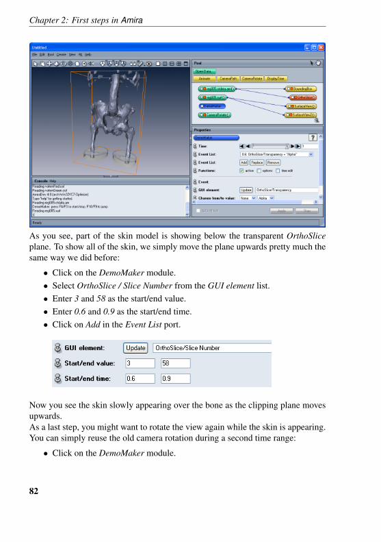
Chapter 2: First steps in Amira
As you see, part of the skin model is showing below the transparent OrthoSliceplane. To show all of the skin, we simply move the plane upwards pretty much thesame way we did before:
• Click on the DemoMaker module.• Select OrthoSlice / Slice Number from the GUI element list.• Enter 3 and 58 as the start/end value.• Enter 0.6 and 0.9 as the start/end time.• Click on Add in the Event List port.
Now you see the skin slowly appearing over the bone as the clipping plane movesupwards.As a last step, you might want to rotate the view again while the skin is appearing.You can simply reuse the old camera rotation during a second time range:
• Click on the DemoMaker module.
82
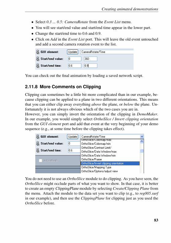
Creating animated demonstrations
• Select 0.3 ... 0.5: CameraRotate from the Event List menu.• You will see start/end value and start/end time appear in the lower part.• Change the start/end time to 0.6 and 0.9.• Click on Add in the Event List port. This will leave the old event untouched
and add a second camera rotation event to the list.
You can check out the final animation by loading a saved network script.
2.11.8 More Comments on Clipping
Clipping can sometimes be a little bit more complicated than in our example, be-cause clipping can be applied to a plane in two different orientations. This meansthat you can either clip away everything above the plane, or below the plane. Un-fortunately it is not always obvious which of the two cases you are in.However, you can simply invert the orientation of the clipping in DemoMaker.In our example, you would simply select OrthoSlice / Invert clipping orientationfrom the GUI element port and add that event at the very beginning of your demosequence (e.g., at some time before the clipping takes effect).
You do not need to use an OrthoSlice module to do clipping. As you have seen, theOrthoSlice might occlude parts of what you want to show. In that case, it is betterto create an empty ClippingPlane module by selecting Create/Clipping Plane fromthe menu. Attach the module to the data set you want to clip (e.g., to reg005.surfin our example), and then use the ClippingPlane for clipping just as you used theOrthoSlice before.
83
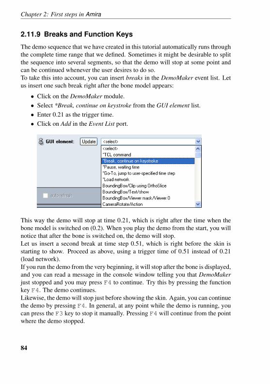
Chapter 2: First steps in Amira
2.11.9 Breaks and Function Keys
The demo sequence that we have created in this tutorial automatically runs throughthe complete time range that we defined. Sometimes it might be desirable to splitthe sequence into several segments, so that the demo will stop at some point andcan be continued whenever the user desires to do so.To take this into account, you can insert breaks in the DemoMaker event list. Letus insert one such break right after the bone model appears:
• Click on the DemoMaker module.• Select *Break, continue on keystroke from the GUI element list.• Enter 0.21 as the trigger time.• Click on Add in the Event List port.
This way the demo will stop at time 0.21, which is right after the time when thebone model is switched on (0.2). When you play the demo from the start, you willnotice that after the bone is switched on, the demo will stop.Let us insert a second break at time step 0.51, which is right before the skin isstarting to show. Proceed as above, using a trigger time of 0.51 instead of 0.21(load network).If you run the demo from the very beginning, it will stop after the bone is displayed,and you can read a message in the console window telling you that DemoMakerjust stopped and you may press F4 to continue. Try this by pressing the functionkey F4. The demo continues.Likewise, the demo will stop just before showing the skin. Again, you can continuethe demo by pressing F4. In general, at any point while the demo is running, youcan press the F3 key to stop it manually. Pressing F4 will continue from the pointwhere the demo stopped.
84
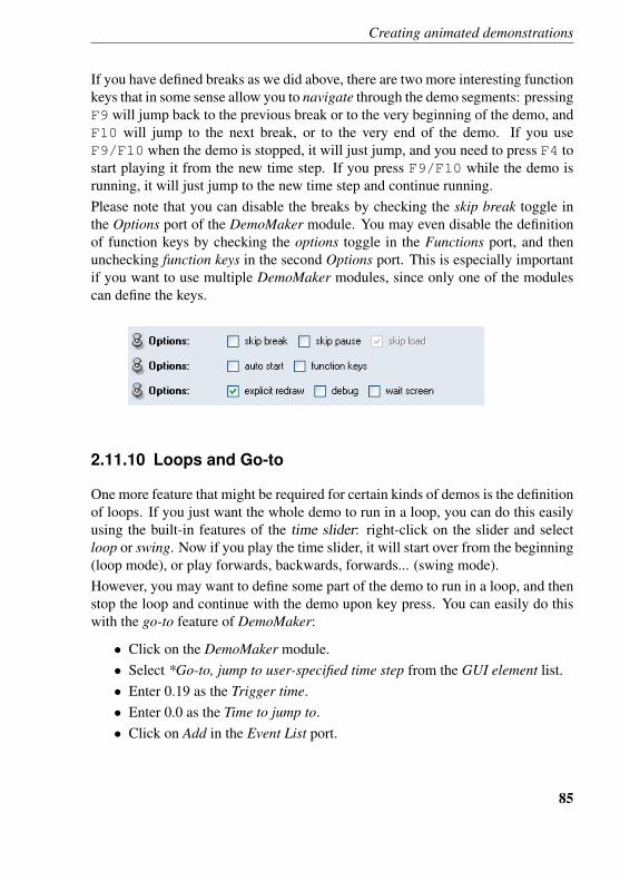
Creating animated demonstrations
If you have defined breaks as we did above, there are two more interesting functionkeys that in some sense allow you to navigate through the demo segments: pressingF9 will jump back to the previous break or to the very beginning of the demo, andF10 will jump to the next break, or to the very end of the demo. If you useF9/F10 when the demo is stopped, it will just jump, and you need to press F4 tostart playing it from the new time step. If you press F9/F10 while the demo isrunning, it will just jump to the new time step and continue running.Please note that you can disable the breaks by checking the skip break toggle inthe Options port of the DemoMaker module. You may even disable the definitionof function keys by checking the options toggle in the Functions port, and thenunchecking function keys in the second Options port. This is especially importantif you want to use multiple DemoMaker modules, since only one of the modulescan define the keys.
2.11.10 Loops and Go-to
One more feature that might be required for certain kinds of demos is the definitionof loops. If you just want the whole demo to run in a loop, you can do this easilyusing the built-in features of the time slider: right-click on the slider and selectloop or swing. Now if you play the time slider, it will start over from the beginning(loop mode), or play forwards, backwards, forwards... (swing mode).However, you may want to define some part of the demo to run in a loop, and thenstop the loop and continue with the demo upon key press. You can easily do thiswith the go-to feature of DemoMaker:
• Click on the DemoMaker module.• Select *Go-to, jump to user-specified time step from the GUI element list.• Enter 0.19 as the Trigger time.• Enter 0.0 as the Time to jump to.• Click on Add in the Event List port.
85
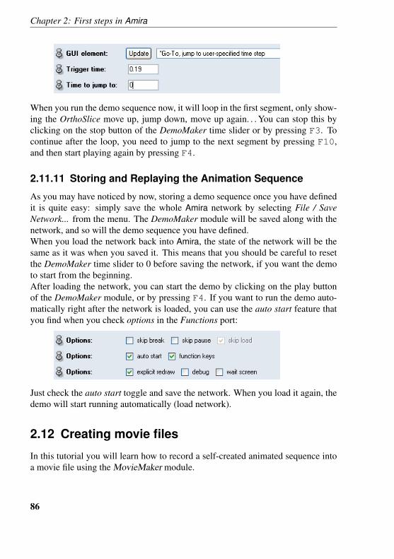
Chapter 2: First steps in Amira
When you run the demo sequence now, it will loop in the first segment, only show-ing the OrthoSlice move up, jump down, move up again. . . You can stop this byclicking on the stop button of the DemoMaker time slider or by pressing F3. Tocontinue after the loop, you need to jump to the next segment by pressing F10,and then start playing again by pressing F4.
2.11.11 Storing and Replaying the Animation Sequence
As you may have noticed by now, storing a demo sequence once you have definedit is quite easy: simply save the whole Amira network by selecting File / SaveNetwork... from the menu. The DemoMaker module will be saved along with thenetwork, and so will the demo sequence you have defined.When you load the network back into Amira, the state of the network will be thesame as it was when you saved it. This means that you should be careful to resetthe DemoMaker time slider to 0 before saving the network, if you want the demoto start from the beginning.After loading the network, you can start the demo by clicking on the play buttonof the DemoMaker module, or by pressing F4. If you want to run the demo auto-matically right after the network is loaded, you can use the auto start feature thatyou find when you check options in the Functions port:
Just check the auto start toggle and save the network. When you load it again, thedemo will start running automatically (load network).
2.12 Creating movie files
In this tutorial you will learn how to record a self-created animated sequence intoa movie file using the MovieMaker module.
86
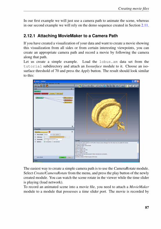
Creating movie files
In our first example we will just use a camera path to animate the scene, whereasin our second example we will rely on the demo sequence created in Section 2.11.
2.12.1 Attaching MovieMaker to a Camera Path
If you have created a visualization of your data and want to create a movie showingthis visualization from all sides or from certain interesting viewpoints, you cancreate an appropriate camera path and record a movie by following the cameraalong that path.Let us create a simple example. Load the lobus.am data set from thetutorial subdirectory and attach an Isosurface module to it. Choose an iso-surface threshold of 70 and press the Apply button. The result should look similarto this:
The easiest way to create a simple camera path is to use the CameraRotate module.Select Create/CameraRotate from the menu, and press the play button of the newlycreated module. You can watch the scene rotate in the viewer while the time slideris playing (load network).To record an animated scene into a movie file, you need to attach a MovieMakermodule to a module that possesses a time slider port. The movie is recorded by
87
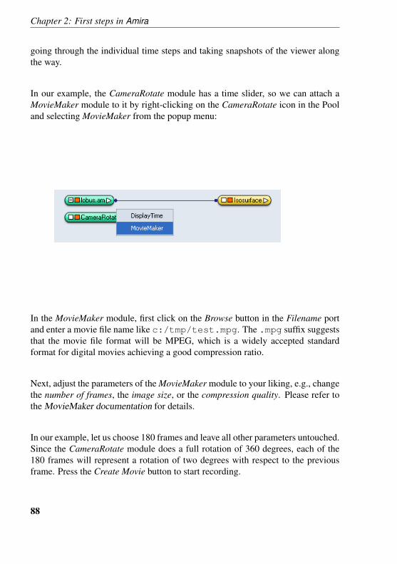
Chapter 2: First steps in Amira
going through the individual time steps and taking snapshots of the viewer alongthe way.
In our example, the CameraRotate module has a time slider, so we can attach aMovieMaker module to it by right-clicking on the CameraRotate icon in the Pooland selecting MovieMaker from the popup menu:
In the MovieMaker module, first click on the Browse button in the Filename portand enter a movie file name like c:/tmp/test.mpg. The .mpg suffix suggeststhat the movie file format will be MPEG, which is a widely accepted standardformat for digital movies achieving a good compression ratio.
Next, adjust the parameters of the MovieMaker module to your liking, e.g., changethe number of frames, the image size, or the compression quality. Please refer tothe MovieMaker documentation for details.
In our example, let us choose 180 frames and leave all other parameters untouched.Since the CameraRotate module does a full rotation of 360 degrees, each of the180 frames will represent a rotation of two degrees with respect to the previousframe. Press the Create Movie button to start recording.
88
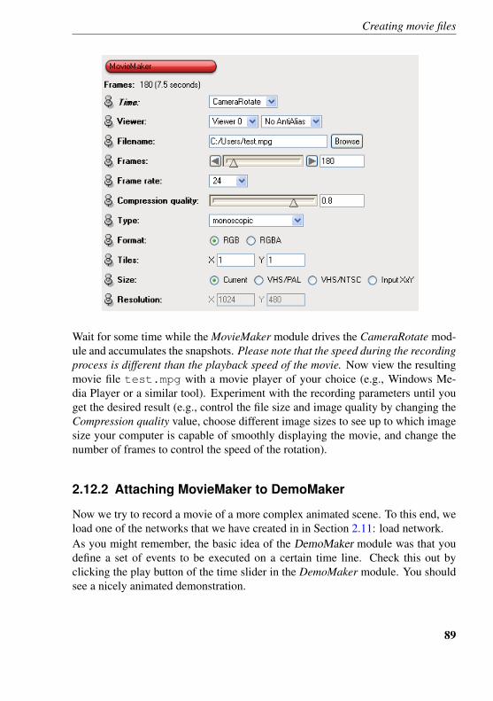
Creating movie files
Wait for some time while the MovieMaker module drives the CameraRotate mod-ule and accumulates the snapshots. Please note that the speed during the recordingprocess is different than the playback speed of the movie. Now view the resultingmovie file test.mpg with a movie player of your choice (e.g., Windows Me-dia Player or a similar tool). Experiment with the recording parameters until youget the desired result (e.g., control the file size and image quality by changing theCompression quality value, choose different image sizes to see up to which imagesize your computer is capable of smoothly displaying the movie, and change thenumber of frames to control the speed of the rotation).
2.12.2 Attaching MovieMaker to DemoMaker
Now we try to record a movie of a more complex animated scene. To this end, weload one of the networks that we have created in in Section 2.11: load network.As you might remember, the basic idea of the DemoMaker module was that youdefine a set of events to be executed on a certain time line. Check this out byclicking the play button of the time slider in the DemoMaker module. You shouldsee a nicely animated demonstration.
89
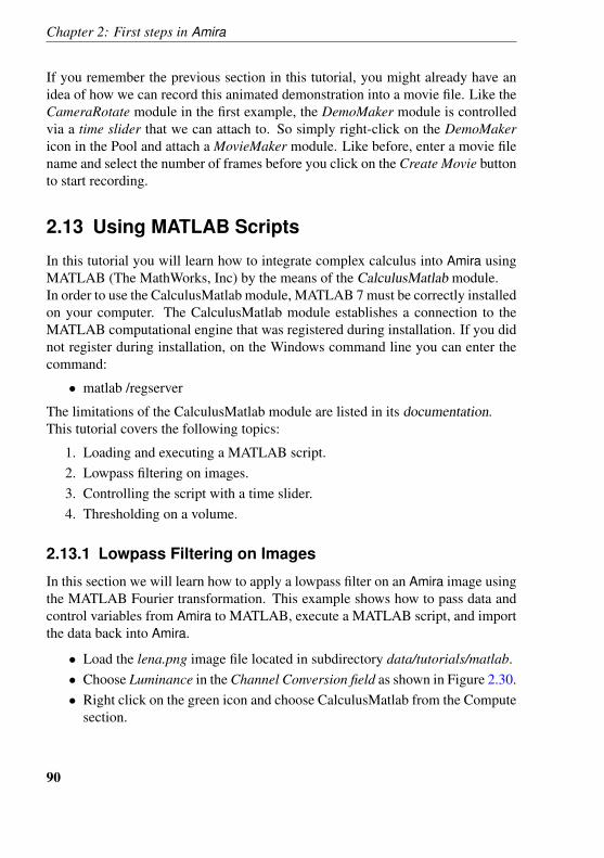
Chapter 2: First steps in Amira
If you remember the previous section in this tutorial, you might already have anidea of how we can record this animated demonstration into a movie file. Like theCameraRotate module in the first example, the DemoMaker module is controlledvia a time slider that we can attach to. So simply right-click on the DemoMakericon in the Pool and attach a MovieMaker module. Like before, enter a movie filename and select the number of frames before you click on the Create Movie buttonto start recording.
2.13 Using MATLAB Scripts
In this tutorial you will learn how to integrate complex calculus into Amira usingMATLAB (The MathWorks, Inc) by the means of the CalculusMatlab module.In order to use the CalculusMatlab module, MATLAB 7 must be correctly installedon your computer. The CalculusMatlab module establishes a connection to theMATLAB computational engine that was registered during installation. If you didnot register during installation, on the Windows command line you can enter thecommand:
• matlab /regserver
The limitations of the CalculusMatlab module are listed in its documentation.This tutorial covers the following topics:
1. Loading and executing a MATLAB script.2. Lowpass filtering on images.3. Controlling the script with a time slider.4. Thresholding on a volume.
2.13.1 Lowpass Filtering on Images
In this section we will learn how to apply a lowpass filter on an Amira image usingthe MATLAB Fourier transformation. This example shows how to pass data andcontrol variables from Amira to MATLAB, execute a MATLAB script, and importthe data back into Amira.
• Load the lena.png image file located in subdirectory data/tutorials/matlab.• Choose Luminance in the Channel Conversion field as shown in Figure 2.30.• Right click on the green icon and choose CalculusMatlab from the Compute
section.
90
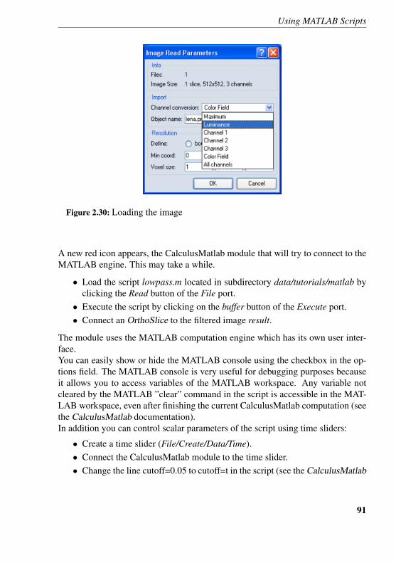
Using MATLAB Scripts
Figure 2.30: Loading the image
A new red icon appears, the CalculusMatlab module that will try to connect to theMATLAB engine. This may take a while.
• Load the script lowpass.m located in subdirectory data/tutorials/matlab byclicking the Read button of the File port.
• Execute the script by clicking on the buffer button of the Execute port.• Connect an OrthoSlice to the filtered image result.
The module uses the MATLAB computation engine which has its own user inter-face.You can easily show or hide the MATLAB console using the checkbox in the op-tions field. The MATLAB console is very useful for debugging purposes becauseit allows you to access variables of the MATLAB workspace. Any variable notcleared by the MATLAB ”clear” command in the script is accessible in the MAT-LAB workspace, even after finishing the current CalculusMatlab computation (seethe CalculusMatlab documentation).In addition you can control scalar parameters of the script using time sliders:
• Create a time slider (File/Create/Data/Time).• Connect the CalculusMatlab module to the time slider.• Change the line cutoff=0.05 to cutoff=t in the script (see the CalculusMatlab
91
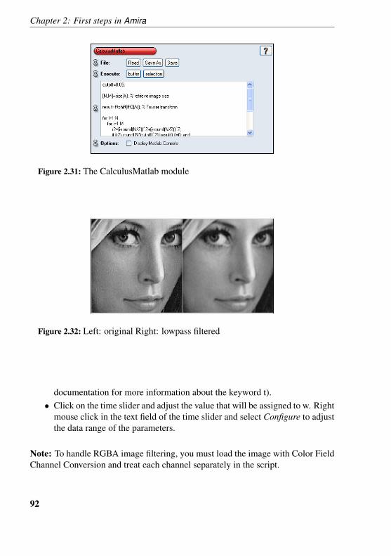
Chapter 2: First steps in Amira
Figure 2.31: The CalculusMatlab module
Figure 2.32: Left: original Right: lowpass filtered
documentation for more information about the keyword t).• Click on the time slider and adjust the value that will be assigned to w. Right
mouse click in the text field of the time slider and select Configure to adjustthe data range of the parameters.
Note: To handle RGBA image filtering, you must load the image with Color FieldChannel Conversion and treat each channel separately in the script.
92
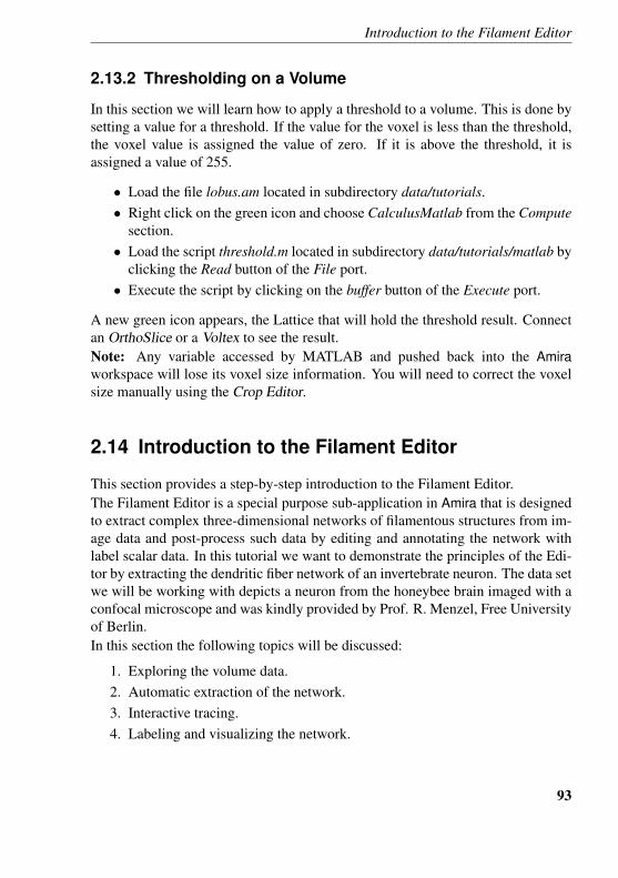
Introduction to the Filament Editor
2.13.2 Thresholding on a Volume
In this section we will learn how to apply a threshold to a volume. This is done bysetting a value for a threshold. If the value for the voxel is less than the threshold,the voxel value is assigned the value of zero. If it is above the threshold, it isassigned a value of 255.
• Load the file lobus.am located in subdirectory data/tutorials.• Right click on the green icon and choose CalculusMatlab from the Compute
section.• Load the script threshold.m located in subdirectory data/tutorials/matlab by
clicking the Read button of the File port.• Execute the script by clicking on the buffer button of the Execute port.
A new green icon appears, the Lattice that will hold the threshold result. Connectan OrthoSlice or a Voltex to see the result.Note: Any variable accessed by MATLAB and pushed back into the Amiraworkspace will lose its voxel size information. You will need to correct the voxelsize manually using the Crop Editor.
2.14 Introduction to the Filament Editor
This section provides a step-by-step introduction to the Filament Editor.The Filament Editor is a special purpose sub-application in Amira that is designedto extract complex three-dimensional networks of filamentous structures from im-age data and post-process such data by editing and annotating the network withlabel scalar data. In this tutorial we want to demonstrate the principles of the Edi-tor by extracting the dendritic fiber network of an invertebrate neuron. The data setwe will be working with depicts a neuron from the honeybee brain imaged with aconfocal microscope and was kindly provided by Prof. R. Menzel, Free Universityof Berlin.In this section the following topics will be discussed:
1. Exploring the volume data.2. Automatic extraction of the network.3. Interactive tracing.4. Labeling and visualizing the network.
93
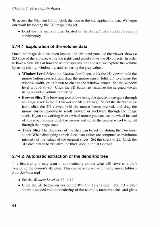
Chapter 2: First steps in Amira
To access the Filament Editor, click the icon in the sub-application bar. We beginour work by loading the 3D image data set.
• Load the file neuron.am located in the data/tutorials/neuronsubdirectory.
2.14.1 Exploration of the volume data
Once the image data has been loaded, the left-hand panel of the viewer shows a2D slice of the volume, while the right-hand panel shows the 3D objects. In orderto have a clear idea of how the neuron spreads out in space, we explore the volumeby using slicing, windowing, and rendering the gray values.
• Window Level Select the Window Level icon, click the 2D viewer, hold themouse button pressed, and drag the mouse cursor left/right to change thewindow width, or up/down to change the window center. Set the windowlevel around 30-80. Click the 3D button to visualize the selected voxelsusing a shaded volume rendering.
• Browse Slice The browsing tool allows using the mouse to navigate throughan image stack in the 2D viewer (or MPR viewer). Select the Browse Sliceicon, click the 2D viewer, hold the mouse button pressed, and drag themouse cursor up/down to scroll forward or backward through the imagestack. If you are working with a wheel mouse you can use the wheel insteadof this icon. Simply click the viewer and scroll the mouse wheel to scrollthrough the image stack.
• Thick Slice The thickness of the slice can be set by sliding the Thicknessslider. When displaying a thick slice, data values are computed as maximumintensity of the values of the original slices. Set thickness to 25. Click the3D slice button to visualize the thick slice in the 3D viewer.
2.14.2 Automatic extraction of the dendritic tree
In a first step you may want to automatically extract what will serve as a draftversion of the neuron’s skeleton. This can be achieved with the Filament Editor’sAuto Skeleton tool.
• Set the Window Level to 37 137.• Click the 3D button on beside the Window Level slider. The 3D viewer
shows a shaded volume rendering of the neuron’s main branches and gives
94
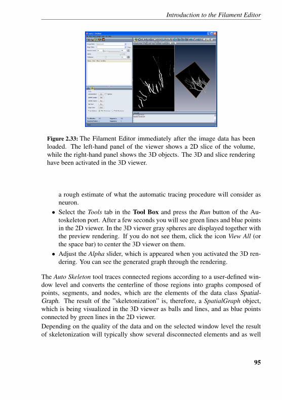
Introduction to the Filament Editor
Figure 2.33: The Filament Editor immediately after the image data has beenloaded. The left-hand panel of the viewer shows a 2D slice of the volume,while the right-hand panel shows the 3D objects. The 3D and slice renderinghave been activated in the 3D viewer.
a rough estimate of what the automatic tracing procedure will consider asneuron.
• Select the Tools tab in the Tool Box and press the Run button of the Au-toskeleton port. After a few seconds you will see green lines and blue pointsin the 2D viewer. In the 3D viewer gray spheres are displayed together withthe preview rendering. If you do not see them, click the icon View All (orthe space bar) to center the 3D viewer on them.
• Adjust the Alpha slider, which is appeared when you activated the 3D ren-dering. You can see the generated graph through the rendering.
The Auto Skeleton tool traces connected regions according to a user-defined win-dow level and converts the centerline of those regions into graphs composed ofpoints, segments, and nodes, which are the elements of the data class Spatial-Graph. The result of the ”skeletonization” is, therefore, a SpatialGraph object,which is being visualized in the 3D viewer as balls and lines, and as blue pointsconnected by green lines in the 2D viewer.Depending on the quality of the data and on the selected window level the resultof skeletonization will typically show several disconnected elements and as well
95
Chapter 2: First steps in Amira
as loops within the networks. Disconnected elements will break the single neuroninto several sub-graphs. Loops, on the other hand, are parts of a graph wheresegments connect onto itself. In some biological objects like e.g. neurons loopsmust not occur. To identify graphs and loops the Filament Editor offers dedicatedtools.
• Press the button Identify Graphs to automatically detect and label all graphsin the SpatialGraph object, that is all connected components. This creates anew label group in the Label Editor named Identified Graphs under whichall identified graphs are listed as Graph1, Graph2, ..., GraphN.
• To visually identify them just click on one of the items in the Identi-fied Graphs list. The selected item is highlighted in red in both viewers.
• Under Identified Graphs select Graph2 and shift-select Graph25, then re-move them by clicking the Delete Selection icon.
• Press again the button Identify Graphs, now you should have only twographs.
• Scale the nodes by moving the Node Scaling Factor slider in the View Op-tions tab of the Tool Box (we will see the details in the next paragraph).
At this point we have only two graphs: Graph0 is the large tree, while Graph1 isjust three segments and four nodes. Switch back to the Tool tab in the Tool Box.
• Select Graph1 in the Label Editor under Identified Graphs• Activate the Select Single icon and Ctrl-click on the closest node of Graph0
in the 3D viewer.• Select the Connect Selected icon to connect the graph.• Press again Identify Graphs. At this point you should have only one graph.• Press Identify Loops to get another label group Identified Loops.• Under Identified Loops select Loop2 and remove it by clicking the Delete
Selection icon. Note that a segment is defined by two nodes. Therefore,when you remove a node the associated segment will be removed too. Inthis example this will not happen, but in general it is very likely that someconnected segments are removed when a loop is deleted.
It should perhaps be noted that the Auto Skeleton tool is also available as a computemodule in the Pool under the Skeleton category. Also, there is a rich set of toolsavailable in the Segmentation Editor to perform the threshold segmentation neces-sary for the skeletonization process. Finally, in the case of a strict tree topology it
96
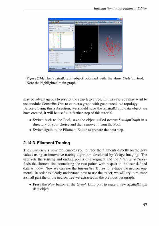
Introduction to the Filament Editor
Figure 2.34: The SpatialGraph object obtained with the Auto Skeleton tool.Note the highlighted main graph.
may be advantageous to restrict the search to a tree. In this case you may want touse module CenterlineTree to extract a graph with guaranteed tree topology.Before closing this subsection, we should save the SpatialGraph data object wehave created, it will be useful in further step of this tutorial.
• Switch back to the Pool, save the object called neuron.Smt.SptGraph in adirectory of your choice and then remove it from the Pool.
• Switch again to the Filament Editor to prepare the next step.
2.14.3 Filament Tracing
The Interactive Tracer tool enables you to trace the filaments directly on the grayvalues using an innovative tracing algorithm developed by Visage Imaging. Theuser sets the starting and ending points of a segment and the Interactive Tracerfinds the shortest line connecting the two points with respect to the user-defineddata window. Now we can use the Interactive Tracer to re-trace the neuron seg-ments. In order to clearly understand how to use the tracer, we will try to re-tracea small part the of the neuron tree we extracted in the previous paragraph.
• Press the New button at the Graph Data port to crate a new SpatialGraphdata object.
97
Chapter 2: First steps in Amira
• Click in the 2D viewer. Using the Browse Slices tool or the mouse wheel,slice through the volume until you reach the root of the neuron.
• Set the thickness of the Thick Slice at 10 for a better visualization.• Activate the Interactive Tracer by clicking the Trace Filament icon in the
toolbar and make sure that the Thick structures option is checked in theTools tab.
Note that the Interactive Tracer is alway active while the Trace Filament icon ishighlighted and it can be triggered only if the 2D viewer is active.If you now move the mouse over the 2D slice, the cursor has a cross shape when-ever it is over black regions and turns into a crosshair (cross within circle) whenit is over voxels that are within the window level. The cross-hair shape indicatesthat it is possible to set tracing key points. As you will see later, when the pointeris over a traced segment (green line) a small ”P” appears in the crosshair. This in-dicates that a click would select the nearest point as a key point. Likewise, an ”N”is shown in the cursor whenever the cursor is over a node and a click will selectthis node as a key point. Furthermore, the cursor turns red when the trace tool isin append mode, meaning that the next click will trigger a tracing action betweenthe previously selected and the current key point.
• Start the tracing by clicking on a gray value of the tree root.• Slice ahead and set further points, until you reach the first bifurcation and
click on it.• Deactivate the Interactive Tracer e.g. by clicking the Select Single tool or
by clicking again its icon.
If you press Identify Graphs graphs, you will see only one graph. You can alsoaccess some statistical information by clicking on Graph Info button in the Toolstab. This opens a spreadsheet window containing a list of all segments in thegraph. The spreadsheet is interactive, i.e. if you click on a line, the correspondingsegment will be highlighted in the viewer.Repeat the actions to trace the first branching sections from the root.
2.14.4 Visualize the network
The SpatialGraph data object is able not only to store the spatial structure, i.e., thegeometry of the network, but also to associate it with scalar and label data.Labels can also be used to tag or annotate sub-graphs according to their topology.
98
Introduction to the Filament Editor
In this simple example we want to tag the three main branches of the Topology asCentral, Left, and Right od a neuron tree.If you already extracted the graph as described in the second subsection you shouldnow load the file you previously saved, otherwise you should go two steps backand read the subsection ”Automatic extraction of the dendritic tree”.
• Right-click into the Label Editor and select Add graph label group.• Right-click on the created label and rename it Topology.• Right-click on the Topology label and select Add label. Repeat this action to
add three labels.• Select and right-click on each of the created labels and rename them Central,
Right, and Left.• Select the Select Lasso icon and select-lasso the right-hand branch. You can
use the Select Lasso tool in combination with Shift key to deselect-lasso orwith the Ctrl key to add elements.
• Right-click on label Right and select Assign selection.• Repeat the last two items to label Central and Left branches. Note that this
is just an exercise, it does not really matter to exactly select the ”Center”,”Right” or ”Left” segments.Select now the View Options tab in the Tool Box
• Scale the nodes using the Scaling Factor slider.• Colorize the nodes according to the label by selecting Topology in Node
Coloring.• Repeat the last item for the segments.• Click on the color button of label Right and select a new color.
For advanced network visualization you can switch to the Pool or Tree View. Ifyou do so, you may attach a SpatialGraphView module to the SpatialGraph objectwe created before.
2.14.5 Alternative way to extract a network using theSegmentation Editor
From the Filament Editor just switch to the Segmentation Editor by clicking theicon in the Sub-application Tool Bar. For an in-depth treatment of the Segmenta-tion Editor we refer you to its documentation and tutorial. For this simple exampleyou may try the following simple steps.
99
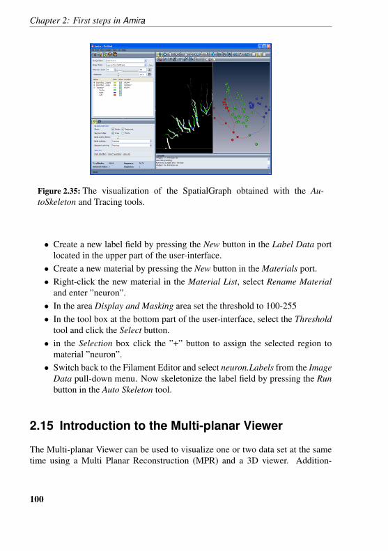
Chapter 2: First steps in Amira
Figure 2.35: The visualization of the SpatialGraph obtained with the Au-toSkeleton and Tracing tools.
• Create a new label field by pressing the New button in the Label Data portlocated in the upper part of the user-interface.
• Create a new material by pressing the New button in the Materials port.• Right-click the new material in the Material List, select Rename Material
and enter ”neuron”.• In the area Display and Masking area set the threshold to 100-255• In the tool box at the bottom part of the user-interface, select the Threshold
tool and click the Select button.• in the Selection box click the ”+” button to assign the selected region to
material ”neuron”.• Switch back to the Filament Editor and select neuron.Labels from the Image
Data pull-down menu. Now skeletonize the label field by pressing the Runbutton in the Auto Skeleton tool.
2.15 Introduction to the Multi-planar Viewer
The Multi-planar Viewer can be used to visualize one or two data set at the sametime using a Multi Planar Reconstruction (MPR) and a 3D viewer. Addition-
100
Introduction to the Multi-planar Viewer
ally, the image volumes can be registered automatically or manually using specificgraphical interfaces.In this tutorial we will try to illustrate how to:
1. Exploration of the volume data, including an associated label field2. Explore two data sets in fusion mode3. Register two data sets
Before we begin our work we need to define the terms Primary and Overlay in thecontext of the Multi-planar Viewer
1. Primary - Reference data set, this data set will be considered our principaldata set to which a secondary data set could be eventually compared or reg-istered. In the context of PET/CT fusion the CT data set would be used asreference data set as it provides the best anatomical reference.
2. Overlay - Secondary data set, which could be compared or registered to thePrimary.
2.15.1 Exploration of the volume data
To activate the Multi-planar Viewer select its icon in the sub-application tool-bar. On a first glance the Multi-planar Viewer looks similar to the Segmen-tation Editor: three slice views, a 3D viewer and a material list. In or-der to start exploring, load the Lobus data set located in the tutorial directorydata/tutorial/lobus.am:
• 3D Volume Rendering Select the 3D Rotate icon (it should have been se-lected by default as you start the Multi-planar Viewer) in the toolbar. Nowrotate the object in the 3D viewer.
• Volume Rendering Modes Try to visualize the volume using VRT or MIPtechniques and their optional rendering modes. To do so, switch betweenthe radio buttons in the 3D Settings panel.
• 3D MPR Click the icon in the 3D Settings panel to activate MPR in the 3Dviewer. You should see now the volume rendered in 3D and the three MPRslices.
• Window Level Select the Window Level icon, click into one of the 2Dviewers, hold the mouse button pressed, and drag the mouse cursor left/rightto change the contrast (window width), or up/down to change the brightness(window center). Note how the bars in the graphical user interface (GUI)
101
Chapter 2: First steps in Amira
change according to the pointer movements. Click in the 3D viewer and dothe same.
• Browse Slice The browsing tool allows using the mouse to navigate throughan image stack in the 2D viewer. Select the Browse Slice icon, click ina 2D viewer, hold the mouse button pressed, and drag the mouse cursorup/down to scroll forward or backward through the image stack. If you areworking with a wheel mouse you can use the wheel to access the browseslice functionality. Simply click once the viewer to activate it and roll themouse wheel to scroll through the image stack.
• Thick Slice The thickness of the slice can be set by sliding the Thicknessslider. When displaying a thick slice, data values are computed as the aver-age, the minimum or the MIP of the values of the included slices, accordingto the selected option.
• Label field Load the associated label field (lobus.label.am) from thetutorial directory and select the checkbox of the Label Field port. Visualizethe materials in 3D with constant color, hide or fade them. Note that theport Label field refers to the Primary data set; to be activated the loadedLabelField has to have the same size as the Primary.
• Extend viewers Double-click one viewer to extend it, double-click to setthe configuration back to 4-window layout again.
Note that clicking the right button in the viewers activates the context menu, whichprovides a quicker way to access tools and settings.
2.15.2 Explore two data sets using fusion mode
The process of image fusion consists of combining relevant information from twoor more images into a single image using different color mappings. The Im-age Fusion became very relevant especially in medical science, where differentimaging modalities can be obtained from the same patient. Typically, the multi-modal imaging includes magnetic resonance (MR), computed tomography (CT),and positron emission tomography (PET/SPECT). Image fusion can be very use-ful in microscopy imaging for alignment and registration of multi-channel, 3D,and 4D data sets.When only one data set is available in the Pool, the Overlay Data port is not avail-able. Load the Lobus2 data set (data/tutorial/lobus2.am) from the tuto-rial directory and the checkbox of the port will become active. Select the Overlaycheckbox and Lobus2 will be shown in the available viewers. Change the min-
102
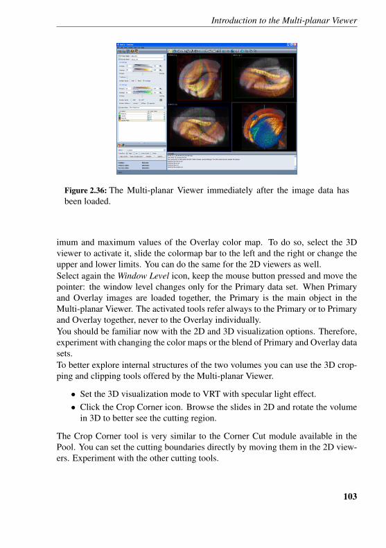
Introduction to the Multi-planar Viewer
Figure 2.36: The Multi-planar Viewer immediately after the image data hasbeen loaded.
imum and maximum values of the Overlay color map. To do so, select the 3Dviewer to activate it, slide the colormap bar to the left and the right or change theupper and lower limits. You can do the same for the 2D viewers as well.Select again the Window Level icon, keep the mouse button pressed and move thepointer: the window level changes only for the Primary data set. When Primaryand Overlay images are loaded together, the Primary is the main object in theMulti-planar Viewer. The activated tools refer always to the Primary or to Primaryand Overlay together, never to the Overlay individually.You should be familiar now with the 2D and 3D visualization options. Therefore,experiment with changing the color maps or the blend of Primary and Overlay datasets.To better explore internal structures of the two volumes you can use the 3D crop-ping and clipping tools offered by the Multi-planar Viewer.
• Set the 3D visualization mode to VRT with specular light effect.• Click the Crop Corner icon. Browse the slides in 2D and rotate the volume
in 3D to better see the cutting region.
The Crop Corner tool is very similar to the Corner Cut module available in thePool. You can set the cutting boundaries directly by moving them in the 2D view-ers. Experiment with the other cutting tools.
103
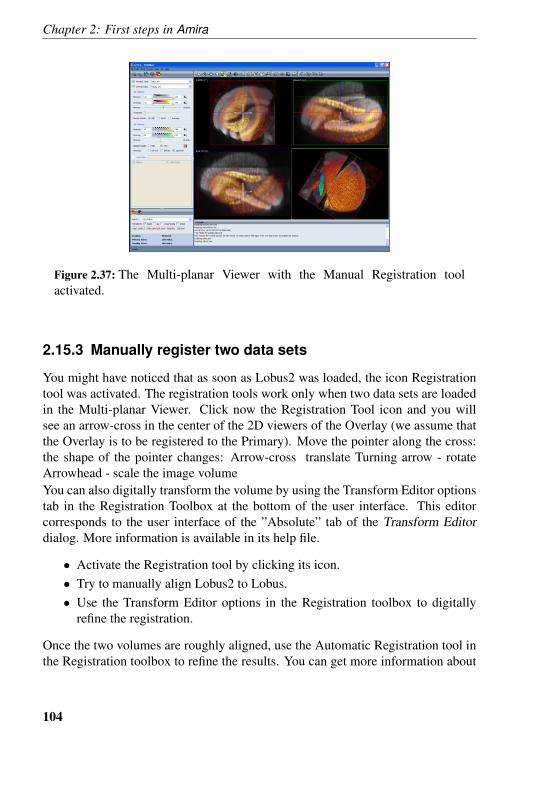
Chapter 2: First steps in Amira
Figure 2.37: The Multi-planar Viewer with the Manual Registration toolactivated.
2.15.3 Manually register two data sets
You might have noticed that as soon as Lobus2 was loaded, the icon Registrationtool was activated. The registration tools work only when two data sets are loadedin the Multi-planar Viewer. Click now the Registration Tool icon and you willsee an arrow-cross in the center of the 2D viewers of the Overlay (we assume thatthe Overlay is to be registered to the Primary). Move the pointer along the cross:the shape of the pointer changes: Arrow-cross translate Turning arrow - rotateArrowhead - scale the image volumeYou can also digitally transform the volume by using the Transform Editor optionstab in the Registration Toolbox at the bottom of the user interface. This editorcorresponds to the user interface of the ”Absolute” tab of the Transform Editordialog. More information is available in its help file.
• Activate the Registration tool by clicking its icon.• Try to manually align Lobus2 to Lobus.• Use the Transform Editor options in the Registration toolbox to digitally
refine the registration.
Once the two volumes are roughly aligned, use the Automatic Registration tool inthe Registration toolbox to refine the results. You can get more information about
104

Introduction to the Multi-planar Viewer
automatic registration by reading the Registration tutorial.
105

3 Program Description
This chapter contains a detailed description of Amira interface components anddata types. No in-depth knowledge of Amira is required to understand the follow-ing sections, but it is a good idea to have a look at one of the tutorials contained inChapter 2, particularly the very first one described in Section 2.1 (Getting Started).
3.1 Interface Components
In this section the following interface components are described:
• File Menu, Edit Menu, Pool Menu, Explorer Menu, Create Menu, ViewMenu, Help Menu• Main Window, Viewer Window, Console Window• File Dialog, Job Dialog, Preferences Dialog, Snapshot Dialog, System In-
formation
3.1.1 File Menu
The file menu lets you load and save data objects as well as Amira network scripts.In addition, it gives you access to Amira’s job dialog and allows you to quit theprogram. In the following text, all menu entries are discussed separately.
3.1.1.1 Open Data
The Open Data button activates Amira’s file dialog and lets you import data setsstored in a file. Most file formats supported by Amira will be recognized automat-ically via the file header or the file name extension. For each file, the file dialogwill display its format. If you try to load a file for which the format couldn’t bedetected automatically, an additional dialog pops up asking you to select the for-mat manually. You may also manually set the file format for any file by selectingthe file, activating the file dialog’s popup menu using the right mouse button, andthen choosing the Format option.
107
Chapter 3: Program Description
A list of all supported file formats is contained in the reference manual. Hints onhow to import your own data sets are given in Section 4.1.If you select multiple files in the file dialog, all of them will be loaded, provided allof them are stored in the same format. 2D images stored in separate files usuallywill be combined into a single 3D data object. On the other hand, there are somefile formats which cause multiple data objects to be created. Finally, you can alsoimport and execute Amira network scripts using the Load button.
3.1.1.2 Open Time Series Data
This button also activates the file dialog, but in contrast to the ordinary Load optionit is assumed that all selected files represent different time steps of a single dataobject. When loading such a time series an instance of a time series control moduleis created. This module provides a time slider allowing you to adjust the currenttime step. Whenever a new time step is selected the corresponding data file is read,and data objects associated with a previous time step are replaced. The module alsoprovides a cache so that the data files only need to be read once provided the cacheis large enough.
3.1.1.3 Save Data
The Save Data button allows you to save a single modified data object again usingthe same filename previously chosen under Save Data As. The button will only beactive if the data object to be saved is selected and if this data object already hasbeen saved using Save Data As. A common application of the Save button is tostore intermediate results during manual segmentation in Amira’s image segmen-tation editor.
3.1.1.4 Save Data As
This button lets you write a data object into a file. To do so you must first selectthe data object (click on the corresponding green data icon). Then choose SaveData As to activate Amira’s file dialog. The file dialog presents a list of all formatssuitable for saving that data object. Choose the one you like and press OK. Notethat you must specify the complete file name including the suffix. Amira will notautomatically add a suffix to the file name. However, it will update the suffixwhenever you select a new format from the file format list. Also, Amira will askyou before it overwrites an existing file.
108
Interface Components
Some file formats create multiple files for a single data object. For example, eachslice of a 3D image data set might be saved as a separate raster file. In this case, thefile name may contain a sequence of hashmarks. This sequence will be replacedby consecutive numbers formatted with leading zeros.If no file format at all has been registered for a certain type of data object, the Saveas button will be disabled. It will also be disabled if more than one data object isselected in the Pool.
3.1.1.5 New Network
This button does a Remove all objects so that you can start building a new networkin the Pool. It also sets the new network name to Untitled.hx.
3.1.1.6 Open Network
The Open Network button activates Amira’s file dialog and lets you load a networkstored in a file. Network files show up in the dialog as being of format ”AmiraScript”. A Remove all objects will be done before the new network is loaded sothat effectively the new network replaces the old network in the Pool. Currentlyonly files with extension .hx can be opened.
3.1.1.7 Save Network
This button allows you to save the complete network of icons and connectionsshown in the Pool. If the network has not been previously saved, you will need tospecify the name of an Amira network script in the file dialog. When executed, thenetwork script restores all data objects and modules as well as the current objecttransformations and the camera settings. The feature is useful for resuming workat a point where it was left in a previous Amira run.Note that usually all data objects must have been stored in a file in order to be ableto save the network. If this is not the case, a dialog is popped up listing all the dataobjects that still need to be saved. In the dialog you can specify that all requireddata objects should be saved automatically in a separate subdirectory.Instead of the option Amira script you can also choose Amira script and data files(pack & go) from the file dialog’s format menu. In this case all data objects cur-rently loaded will be saved in a separate directory. More options affecting theexport of network scripts can be adjusted in the Preferences dialog.
109

Chapter 3: Program Description
3.1.1.8 Save Network As
This button works like the Save Network button except that in this case you willalways need to specify the name of an Amira network script in the file dialog.
3.1.1.9 Recent Files
This button can be used to load recently used files. When choosing this menuentry a submenu appears listing the five most recent files. If multiple 2D imageshave been loaded this is indicated with the name of the first file followed by threeperiods (...).
3.1.1.10 Recent Networks
This button can be used to load recently used network scripts. When choosing thismenu entry a submenu appears listing the five most recent network scripts.
3.1.1.11 Jobs
This button brings up Amira’s job dialog which is used to control the executionof batch jobs running in the background. For example, tetrahedral grids can begenerated in a batch job (see module TetraGen). However, for most users thebatch queue will be of minor interest.
3.1.1.12 Quit
This button terminates Amira. The current network configuration will be lost un-less you explicitly save it using Save Network.
3.1.2 Edit Menu
The Edit menu provides access to the standard cut/copy/paste/delete commands, aswell as to an extended version of the Parameter Editor and the Amira preferencesdialog.
3.1.2.1 Cut
In the Console, this command cuts selected text and copies it to the clipboard. Inthe Pool, this command removes the selected objects.
110
Interface Components
3.1.2.2 Copy
In the Console, this command copies the selected text to the clipboard. In the Pool,this command has no effect.
3.1.2.3 Paste
In the Console, this command pastes the text in the clipboard to the current textinsertion point. In the Pool, this command has no effect.
3.1.2.4 Delete
In the Console, this command deletes the selected text. In the Pool, this commanddeletes the selected objects.
3.1.2.5 Select All
In the Pool, this command select all objects.
3.1.2.6 Database
The Database button activates an extended version of the Parameter Editor, al-lowing you to manipulate Amira’s global parameter database. Among others, theparameter database contains a set of predefined materials (to be used for imagesegmentation and surface reconstruction) and of predefined boundary ids (to beused for surface editing and FEM pre-processing). For example, for each materialand for each boundary id a default color can be defined in the database.Modification, insertion, and removal of parameters is performed in the sameway as in the ordinary parameter editor. In addition, the extended parame-ter dialog provides a menu bar allowing you to load, import, save, or searchthe global parameter database. Amira’s default database is stored in the fileshare/materials/database.hm located in the directory where Amira wasinstalled. Use the Database menu option Set default file to specify that a differentdatabase file be used instead. This change is permanent, i.e., it takes effect also ifAmira is restarted. To switch back to the system default, use the Database menuoption Use system default file.
111
Chapter 3: Program Description
3.1.2.7 Preferences
This option opens the Amira preferences dialog described in Section 3.1.13. Thedialog controls how network scripts are exported. It also lets you choose if warningdialogs should be popped up if you try to delete data objects which have not yetbeen saved to file, or if you try to exit Amira without having saved the currentnetwork before. Possibly most interesting, it allows you to configure the layout ofyour Amira window.
3.1.3 Pool Menu
The Pool menu is displayed if ”graph view” is selected. This selection is madeusing the the Layout tab of the Edit/Preferences menu.The Pool menu provides control over the visibility of object icons and lets youdelete or duplicate objects. Depending on how many icons are selected in thePool, some menu options might be disabled.
3.1.3.1 Hide
The Hide button hides all currently selected objects. The object’s icons are re-moved from the Pool but the objects themselves are retained. You get the sameeffect by pressing the Ctrl-H key. Hidden objects can be made visible againusing Show or Show All.
3.1.3.2 Remove
The Remove button deletes all selected objects and removes the correspondingicons from the Pool. You can get the same effect by pressing Ctrl-X. If youwant to reuse a data object later on, be sure to save it in a file before deletingit. If a data object has been modified but has not yet been saved to a file, it ismarked by a little asterisk in the object icon. In the Preferences dialog you canchoose whether a warning dialog should be printed if you try to delete unsaveddata objects which cannot be recomputed by an up-stream compute module. If youdelete a data object, all connected modules will be deleted as well. However, ifyou delete a module connected data objects (e.g., the results of a compute module)will be retained.
112
Interface Components
3.1.3.3 Duplicate
The Duplicate button creates copies of all selected data objects. For each copya new data icon is put in the Pool. The name of a duplicated data object differsfrom the original one by one or more appended digits. The duplicate option is notavailable if you have selected icons that do not represent data objects (e.g., displayor compute modules).
3.1.3.4 Rename
This button allows you to change the name of a selected object in a small dialogbox which is popped up when the button is pressed. If no object is selected or ifmultiple objects are selected the button is disabled. Note that no two objects inAmira can have the same name. Therefore, the name entered in the dialog may bemodified by appending digits to it, if necessary. The dialog can also be raised bypressing the F2 key on a selected object into the pool.
3.1.3.5 Show
The Show button allows you to make hidden objects visible, so that their icons aredisplayed in the Pool. Among the hidden objects there are usually some colormapswhich are loaded at start-up. This option will be unavailable if there are no hiddenobjects.
3.1.3.6 Show All
The Show All button makes all currently hidden objects visible, so that their iconsare displayed in the Pool. This option will be unavailable if there are no hiddenobjects.
3.1.3.7 Remove All
The Remove All button deletes all currently visible icons and the associated objectsfrom the Pool. A pre-loaded colormap that is currently visible is also deleted, butall hidden objects are retained. If you select the option check if data objects needto be saved in the Preferences dialog, a warning dialog is popped up if there aredata objects which have not yet been saved to a file.
113
Chapter 3: Program Description
3.1.3.8 Duplicate mode
This mode is applicable when multiple modules of the same type will be attachedto a single data object. If the toggle is on, the port values of the first module willbe used to initialize the port values of subsequently attached modules. This can beconvenient if you want the modules to have the same initial port values.Example: Attach an Orthoslice to your data object and set the Mapping type to”Colormap” and the colormap range to 0-3. If you attach another Orthoslice tothe same data object, its Mapping type will be ”Colormap” and its colormap rangewill be 0-3.
3.1.3.9 Auto adjust range of colormaps
If this toggle is on, requests that Amira automatically adjust the range of a col-ormap to correspond to the data range of the data set it is connected to. Note thatthis feature only applies to the seismic modules: seismic slices Inline, Crossline,TimeSlice, etc., CroppedVolume, and SeismicSurfaceView.
3.1.4 Explorer Menu
The Explorer menu is displayed if ”tree view” is selected. This selection is madeusing the the Layout tab of the Edit/Preferences menu.The Explorer menu is identical to the Pool menu except that the Show, Show All,and Hide items are not available.See the Pool menu description for complete details.
3.1.5 Create Menu
The Create menu lets you create modules or data objects that cannot be accessedvia the popup menu of any other object. The Create menu provides different cat-egories like the popup menu in the Pool. For example, you can create a procedu-rally defined scalar field (where you can type in some arithmetic expression) bychoosing Scalarfield from the Data sub-menu. The icon of a newly created objectusually will not be connected to any other object in the Pool. In order to establishconnections later on, use the popup menu over the small white square on the leftside of the object’s icon. You can also put in links to scripts in the Create menu.Details are defined in Section 5.5 (Configuring popup menus).
114
Interface Components
3.1.6 View Menu
The View menu provides control over several Viewer options affecting the displayindependent of the Viewer input.
3.1.6.1 Layout
The Layout button lets you select between one, two, or four 3D viewers. Allviewers will be placed inside a common window using a default layout. If youwant to create an additional viewer in a separate window, choose Extra Viewer.You may create even more viewers using the Tcl command viewer <n> show.Starting from n=4, viewers will be placed in separate windows.
3.1.6.2 Background
The Background button opens the background dialog, allowing you to switch be-tween the different background styles uniform, gradient, and checkerboard. Inaddition, the dialog allows you to adjust the two colors used by these styles.In order to change the background color via the command interface, use theviewer commands viewer <n> setBackgroundColor and viewer <n>setBackgroundColor2. The command interface also allows you to placean arbitrary raster image into the viewer background (see Section 5.3.3.1, viewercommands).
3.1.6.3 Transparency
The Transparency button controls the way of calculating pixel values with respectto object transparencies during the rendering process.
• Screen Door: Transparent surfaces are approximated using a stipple pattern.• Add: Additive alpha blending.• Add Delayed: Additive alpha blending with two rendering passes. Opaque
objects come first and transparent objects come second.• Add Sorted: Like Add Delayed, but transparent objects are sorted by dis-
tances of bounding box centers from the camera and are rendered in back-to-front order.
• Blend: Multiplicative alpha blending.
115
Chapter 3: Program Description
• Blend Delayed: Multiplicative alpha blending with two rendering passes.Opaque objects come first and transparent objects come second.
• Blend Sorted: Like Blend Delayed, but transparent objects are sorted bydistances of bounding box centers from the camera and are rendered in back-to-front order.
• Sorted Layers: Uses a fragment-level depth sorting technique, which givesbetter results for complex transparent objects. Multi-Texture, Texture Envi-ronment Combine, Depth texture, and Shadow OpenGL extensions must besupported by your graphics board. If the graphics board does not supportthese extensions, behaves as if Blend Sorted was set.
• Sorted Layers Delayed: Like Sorted Layers, but rendering all transparentobjects after opaque ones.
3.1.6.4 Lights
The Lights menu lets you activate different light settings for the 3D viewer. Bydefault, the viewer uses a single headlight, i.e., a directional light pointing in al-most the same direction as the camera is looking. The headlight can be switchedon or off in each viewer via the viewer’s popup menu. Alternatively, the head-light can be switched on or off for all viewers using the headlight toggle inthis Lights menu. This standard light settings can be restored using the Stan-dard button. More light settings can be defined by creating an appropriate filein $AMIRA ROOT/share/lights. By default, Amira provides one additionallight setting including colored lights (BlueRed).At any time, additional lights can be created via the Create light option. Exceptfor the viewer’s default headlight, all lights are represented by little blue icons inthe Pool, just like ordinary data objects or modules. In order to make all hiddenlight icons visible, use the Show all icons option. Hide all icons hides the icons ofall light objects. For more information about lights, please refer to the ReferenceSection of this manual.
3.1.6.5 Fog
The Fog button introduces a fog effect into the displayed scene and controls howopacity increases with distance from the camera. The fog effect will only be seenon a uniform background. More fine tuning is provided by the fogRange Viewercommand.
116
Interface Components
• None: No fog effect (default).• Haze: Linear increase in opacity with distance.• Fog: Exponential increase in opacity with distance.• Smoke: Exponential squared increase in opacity with distance.
3.1.6.6 Axis
The Axis button creates an Axis module named GlobalAxis which immediatelydisplays a coordinate frame in the viewer window. This button is a toggle, soclicking on it again deletes the GlobalAxis module and removes the coordinateframe from the viewer window. The axes will be centered at the origin of the worldcoordinate system. You may also create local axes by selecting the appropriateentry from a data object’s popup menu.
3.1.6.7 Measuring
The Measuring button creates an instance of a Measuring module that lets youmeasure distances and angles on objects within the viewer.
3.1.6.8 Easy Fade
The Easy Fade toggle lets you switch on a fading effect which is applied to allkinds of scene movements. Before a new image is rendered only a certain fractionof the background will be cleared. In this way older images remain visible untilthey fade out after a while. Note that this mode requires single buffer rendering,and therefore, flickering may be visible in some cases.
3.1.6.9 Frame Counter
The Frame Counter toggle lets you switch on a frames-per-second counter thatwill be displayed in the first viewer (viewer 0).
3.1.6.10 Console
The Console toggle lets you switch on or off display of the Console window.
117
Chapter 3: Program Description
3.1.7 Online Help
Amira user’s documentation is available online. You can access it via the User’sGuide entry of the main window’s Help menu. The user’s guide contains someintroductory chapters, as well as a reference section containing documentation forspecific
• modules• data types• editors• file formats• and other components
You may access the documentation of any such object via a separate index pageaccessible from the home page of the online help browser. Amira modules alsoprovide a question mark button in the Properties Area. Pressing this button directlypops up the help browser for the particular module.By default, the help browser is displayed in its own top-level window, but you caneasily integrate it into the console pane. In this case, a tab button allows you toswitch between the Console and the Help window. To change the way the helpbrowser is displayed, use the Layout tab of the Edit/Preferences menu.Going through the online documents is similar to text handling within any otherhypertext browser. In fact, the documentation is stored in HTML format and canbe read with a standard web browser as well. Some specially marked (colored andunderlined) text items allow you to jump quickly to related or referenced topics,where blue items point to unread sections, and red items to already viewed sec-tions. Use the Backward and Forward buttons to scroll in the document historyand Home to move to the first page.Searching the online documentationThe online help browser provides a very simple interface for a content and fulltext search. If you want to search through the complete documentation, enter thedesired text into the text field. Pressing CTRL-SHIFT-F moves the focus to thistext field and marks all text in this field for quick access. The search will beperformed upon pressing the Enter key.The search is done by using the complete search phrase. For example, supposeyou are looking for information about the surface editor the output shows the pagetitle where the phrase is contained and a small text surrounding the search phrase.
118
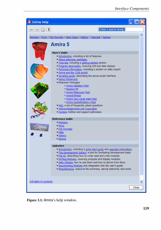
Interface Components
Figure 3.1: Amira’s help window.
119
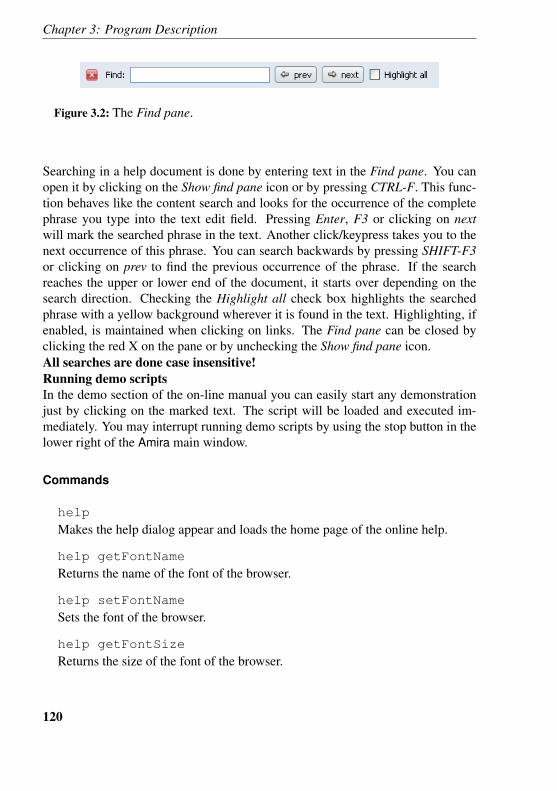
Chapter 3: Program Description
Figure 3.2: The Find pane.
Searching in a help document is done by entering text in the Find pane. You canopen it by clicking on the Show find pane icon or by pressing CTRL-F. This func-tion behaves like the content search and looks for the occurrence of the completephrase you type into the text edit field. Pressing Enter, F3 or clicking on nextwill mark the searched phrase in the text. Another click/keypress takes you to thenext occurrence of this phrase. You can search backwards by pressing SHIFT-F3or clicking on prev to find the previous occurrence of the phrase. If the searchreaches the upper or lower end of the document, it starts over depending on thesearch direction. Checking the Highlight all check box highlights the searchedphrase with a yellow background wherever it is found in the text. Highlighting, ifenabled, is maintained when clicking on links. The Find pane can be closed byclicking the red X on the pane or by unchecking the Show find pane icon.All searches are done case insensitive!Running demo scriptsIn the demo section of the on-line manual you can easily start any demonstrationjust by clicking on the marked text. The script will be loaded and executed im-mediately. You may interrupt running demo scripts by using the stop button in thelower right of the Amira main window.
Commands
help
Makes the help dialog appear and loads the home page of the online help.
help getFontName
Returns the name of the font of the browser.
help setFontName
Sets the font of the browser.
help getFontSize
Returns the size of the font of the browser.
120
Interface Components
help setFontSize
Sets the size of the font of the browser. In order to permanently change thefont size, put this command in the .Amira file in your home directory or in anAmira.init file in the current working directory. For details see Section 4.4.
help load file.html
Load the specified hypertext document in the file browser. Note that only asubset of HTML is supported.
help reload
Reload the current document.
3.1.8 Main Window
Amira’s Main window consists of two components: the sub-application Pool orExplorer in the upper part of the window, and the Properties Area in the lowerpart.The Pool contains icons representing data objects and modules currently in useas well as lines connecting icons indicating dependencies between objects andmodules. Like the Pool, the Explorer contains icons representing data objects andmodules currently in use. However this information is displayed in a tree view.The user can choose to use either display type by selecting the icons in the Sub-application Toolbar In ”graph view” mode, the Pool is displayed. In ”tree view”mode, the Explorer is displayed.Note: Other than when attention is being specifically called to highlight the dif-ferences between the Pool (Pool View) and the Explorer (Tree View), ”Pool” willbe used throughout the Amira documentation to refer generically to the upper paneof the main Amira window containing the collection of objects and modules thatdefine the visualization network.The Properties Area is the place where the user interface of selected objects isdisplayed. Typically, the interface consists of buttons and sliders arranged in Ports.They can be thought of as ports because the user can pass information to a modulethrough them. The Pool and the Properties Area are described below.By default, the Main Window, the Viewer window, the Console window, and theHelp browser are all panes of a single large Amira window. However, it is possibleto designate that any of these last three components be displayed in its own top-level window using the Layout tab of the Edit/Preferences menu.
121
Chapter 3: Program Description
3.1.8.1 Pool (Graph View)
ConceptsThe Pool is displayed if ”graph view” is selected. This selection is made using thethe Layout tab of the Edit/Preferences menu.Once a data object has been loaded or a module has been created, it will be repre-sented by an icon in the Pool. Some objects, especially initially loaded colormaps,may not be visible here. Such hidden objects are listed in the Pool/Show Objectmenu of the Main Window. Selecting an object from this menu causes the corre-sponding icon to be made visible in the Pool.Icon colors are used indicate different types of objects. Data objects are shown ingreen and are the only objects which can be saved to disk using File/Save. Com-putational modules are shown in red, visualization modules are yellow, and visu-alization modules of slicing type are orange. Such modules may be used to clipthe graphical output of any other module.Connections between data objects and processing modules, shown as blue lines,represent the flow of data. For display modules, these connections show the dataused to generate the display. You may connect or disconnect objects by pickingand dragging a blue line between object icons.As you might expect, not all types of processing modules are applicable to allkinds of data objects. If you click on a data object icon with the right mousebutton, a menu pops up that shows all types of modules that can be connected tothat object. (Alternatively, you can click on the small white triangle on the rightside of the icon with the left, right, or middle button.) Selecting one of the moduleswill automatically create an instance of that module type and connect it to the dataobject. A new icon and a connecting line will appear in response. This way youcan set up a more or less complex network that represents the computational stepsrequired to carry out a specific visualization task and is used to trigger them. Notethat modules used will appear as shortcut (or macro) buttons in the upper part ofthe window.If you look closer at an object’s icon you will notice two small squares on its left,one white and one orange. If you click on the white square with the left (or right,or middle) mouse button, a menu pops up that shows all connection ports of thatobject.If the white square has a ”-” or a ”+” inside, you can click it with the left (or right,or middle) mouse button to hide (”collapse”) or unhide the objects connected tothat object. The collapse feature is helpful if there are too many objects in the Poolto view easily at once. The hidden objects will be visible in the Pool/Show Object
122
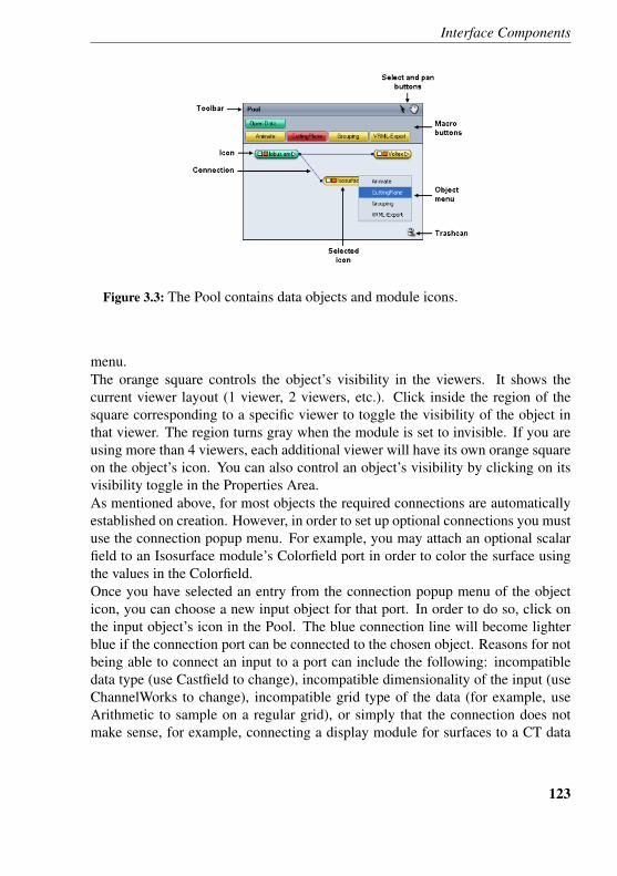
Interface Components
Figure 3.3: The Pool contains data objects and module icons.
menu.The orange square controls the object’s visibility in the viewers. It shows thecurrent viewer layout (1 viewer, 2 viewers, etc.). Click inside the region of thesquare corresponding to a specific viewer to toggle the visibility of the object inthat viewer. The region turns gray when the module is set to invisible. If you areusing more than 4 viewers, each additional viewer will have its own orange squareon the object’s icon. You can also control an object’s visibility by clicking on itsvisibility toggle in the Properties Area.As mentioned above, for most objects the required connections are automaticallyestablished on creation. However, in order to set up optional connections you mustuse the connection popup menu. For example, you may attach an optional scalarfield to an Isosurface module’s Colorfield port in order to color the surface usingthe values in the Colorfield.Once you have selected an entry from the connection popup menu of the objecticon, you can choose a new input object for that port. In order to do so, click onthe input object’s icon in the Pool. The blue connection line will become lighterblue if the connection port can be connected to the chosen object. Reasons for notbeing able to connect an input to a port can include the following: incompatibledata type (use Castfield to change), incompatible dimensionality of the input (useChannelWorks to change), incompatible grid type of the data (for example, useArithmetic to sample on a regular grid), or simply that the connection does notmake sense, for example, connecting a display module for surfaces to a CT data
123
Chapter 3: Program Description
set.In order to disconnect an input object click on the icon of the module the portbelongs to. Data objects possess a special connection port called Master. Thisport refers to a computational module or editor the data object is attached to. Itindicates that the computational module or editor controls the data object, i.e., thatit may modify its contents.Each object has an associated control panel containing buttons and sliders for set-ting or changing additional parameters of the object. The control panel becomesvisible once the object has been selected, i.e. by clicking on its icon with the leftmouse button. In order to select multiple objects, you can shift-click the corre-sponding icons or select them by using the rectangular selection tool (press andhold down the left mouse button over the Pool background, then sweep out a rect-angle). Clicking on the icon of a selected object deselects it again. Clicking some-where on the background of the Pool causes all selected objects to be deselected.One or more selected icons may be dragged around in the Pool by clicking on themand moving the mouse pointer while holding down the mouse button.InterfaceAt the right of the Pool banner are the PoolSelect (arrow) and PoolPan (hand) but-tons. In PoolSelect mode, the mouse is used for selecting, positioning, connecting,and disconnecting objects in the Pool. In PoolPan mode, moving the mouse pansthe Pool workspace. Press the Control key to switch temporarily from one modeto the other.At the top of the Pool is a region containing shortcut (or macro) buttons. The OpenData button is a shortcut to the File/Open Data menu item. Up to 4 additionalbuttons are automatically displayed depending on the currently selected object(s).They provide easy access to the modules that are most commonly used and/or thathave been recently used with the currently selected object.The trashcan at the bottom right of the Pool provides a convenient shortcut forremoving an object. Drag the object to the trashcan. When the cursor turns intoan ”X”, release the mouse button and the object will be removed from the Pool.If you remove a data object, all modules downstream from that module will bedeleted as well. Alternatively, you can use the Remove object item from the Poolmenu, or you can use the Delete key or Ctrl-x to remove a selected object.
3.1.8.2 Explorer (Tree View)
The Explorer is displayed if ”Tree View” is selected in the Sub-application Tool-bar.
124
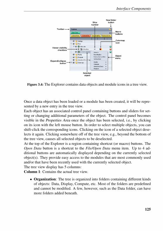
Interface Components
Figure 3.4: The Explorer contains data objects and module icons in a tree view.
Once a data object has been loaded or a module has been created, it will be repre-sented by a new entry in the tree view.Each object has an associated control panel containing buttons and sliders for set-ting or changing additional parameters of the object. The control panel becomesvisible in the Properties Area once the object has been selected, i.e., by clickingon its icon with the left mouse button. In order to select multiple objects, you canshift-click the corresponding icons. Clicking on the icon of a selected object dese-lects it again. Clicking somewhere off of the tree view, e.g., beyond the bottom ofthe tree view, causes all selected objects to be deselected.At the top of the Explorer is a region containing shortcut (or macro) buttons. TheOpen Data button is a shortcut to the File/Open Data menu item. Up to 4 ad-ditional buttons are automatically displayed depending on the currently selectedobject(s). They provide easy access to the modules that are most commonly usedand/or that have been recently used with the currently selected object.The tree view display has 5 columns:Column 1: Contains the actual tree view.
• Organization: The tree is organized into folders containing different kindsof objects: Data, Display, Compute, etc. Most of the folders are predefinedand cannot be modified. A few, however, such as the Data folder, can havemore folders added beneath.
125
Chapter 3: Program Description
Currently, there are two ”templates” that control the organization of thetree view: a default template for most Amira users, and a ”geoscience”template that includes predefined folders for 3D surveys, horizons, faults,etc. The user can choose the desired template using the Layout tab of theEdit/Preferences menu.
• Connections: If you click on a data object icon with the right mouse button,a menu pops up that shows all types of modules that can be connected to thatobject. Selecting one of the modules will automatically create an instanceof that module type and connect it to the data object. A new item in thetree view will appear in response. In this way you can set up a more orless complex network that represents the computational steps required tocarry out a specific visualization task and is used to trigger them. Note thatmodules used will appear as shortcut (also known as ”macro”) buttons inthe upper part of the window.For most objects the required connections are automatically established oncreation. The connection is shown in the connected object’s input port in itscontrol panel in the Properties Area. For example, when you attach a TimeS-lice to my data.lda, in the Data port of the TimeSlice control panel, youwill see ”my data.lda” in the pulldown list. If other objects in the Explorercan be connected to the TimeSlice, they will be in the list as well. To switchthe connection, simply select a different item from the list. The tree view(and possibly the viewer display) will be updated accordingly. Selecting”NO SOURCE” from the list disconnects the module from any object.Reasons for not being able to connect an input to a port can include the fol-lowing: incompatible data type (use Castfield to change), incompatible di-mensionality of the input (use ChannelWorks to change), incompatible gridtype of the data (for example, use Arithmetic to sample on a regular grid),or simply that the connection does not make sense, for example, connectinga display module for surfaces to a volume data set.Data objects possess a special connection port called Master. This portrefers to a computational module or editor the data object is attached to. Itindicates that the computational module or editor controls the data object,i.e., that it may modify its contents.
126
Interface Components
• Expand/Collapse: You can click on the + and - icons to expand or collapserespectively a portion of the tree.
• Drag-and-Drop: You can use drag-and-drop to move items in the tree view.For example, to connect an existing visualization module to a different dataset, you can drag and drop it from its current location onto a compatibledata set. Drag-and-drop does not work for disconnecting objects. You mustuse the connection ports for this.
• Viewer Toggle: The check boxes control the visibility of the object inthe currently active viewer. If there are multiple viewers, e.g., a 4-viewerlayout, you can select a viewer to be active, set the object’s visibility inthat viewer, then repeat as often as necessary to set the desired visibilityin each viewer. However, it will probably be more convenient to controlthe visibility in individual viewers by using the viewer toggle button in theobject’s control panel in the Properties Area. The viewer toggle button isthe orange square just to the right of the module name in its control panel.The button is divided into regions corresponding to the current viewerlayout. Click on the region to toggle visibility of the object on/off in thecorresponding viewer. If there are more than 4 viewers, each additionalviewer will have it own toggle button.
• Adding a Folder: At the right of the Explorer banner is the TVNewFolderbutton used for adding a new folder directly below the currently selectedfolder. You can also add a folder by right clicking on an existing folder andselecting New Folder from the context menu. At some positions in the tree,it may not be possible to add a new folder.
• Removing an Object: To remove one or more objects from the Explorer,first select the object(s) to be removed. You can then use the Remove objectitem from the Explorer context menu, or you can press the Delete key orCtrl-x to remove a selected object. If you remove a data object, all modulesdownstream from that module will be deleted as well.
127
Chapter 3: Program Description
• Hovering: Hovering the mouse over an item in the tree view displays infor-mation about item, usually its type, e.g., HxUniformScalarField3.
Column 2: Shows, for certain objects, the current value of a port of interest.Currently, the slice number is shown for slice modules (OrthoSlice, Inline, etc.)and the Time Scale Factor is shown for the SeismicSettings module.
Column 3: Shows the current colormap, if any, associated with the module orobject. You can right click on it to bring the standard colormap context menu. Oryou can left click on it to bring up the Colormap Editor.
Column 4: Displays the icon of the editor, if any, currently operating on theobject. For example, the Crop Editor, the Parameter Editor, etc.
Column 5: Displays a colored-coded marker indicating the kind of object or mod-ule, as follows:
• Red – computational modules
• Orange – visualization modules of slicing type. These modules may beused to clip the graphical output of any other module.
• Yellow – visualization modules
• Green – data objects. These are the only objects which can be saved to diskusing File/Save.
• Blue – script objects
• Purple – settings modules, e.g., SeismicSettings, LDAExpertSettings, etc.
128
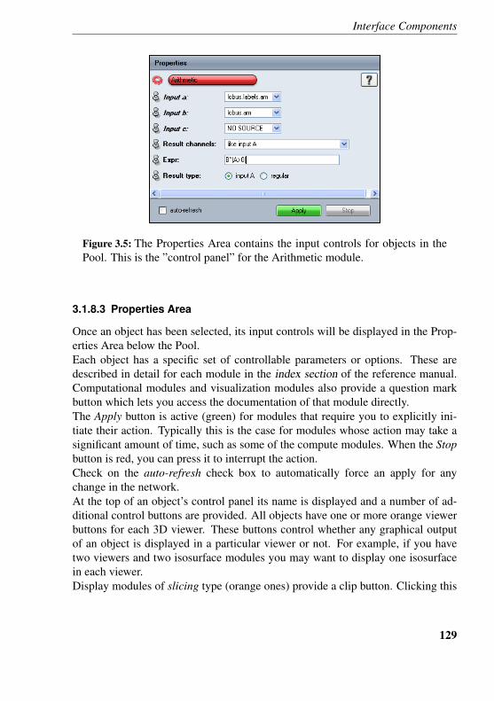
Interface Components
Figure 3.5: The Properties Area contains the input controls for objects in thePool. This is the ”control panel” for the Arithmetic module.
3.1.8.3 Properties Area
Once an object has been selected, its input controls will be displayed in the Prop-erties Area below the Pool.Each object has a specific set of controllable parameters or options. These aredescribed in detail for each module in the index section of the reference manual.Computational modules and visualization modules also provide a question markbutton which lets you access the documentation of that module directly.The Apply button is active (green) for modules that require you to explicitly ini-tiate their action. Typically this is the case for modules whose action may take asignificant amount of time, such as some of the compute modules. When the Stopbutton is red, you can press it to interrupt the action.Check on the auto-refresh check box to automatically force an apply for anychange in the network.At the top of an object’s control panel its name is displayed and a number of ad-ditional control buttons are provided. All objects have one or more orange viewerbuttons for each 3D viewer. These buttons control whether any graphical outputof an object is displayed in a particular viewer or not. For example, if you havetwo viewers and two isosurface modules you may want to display one isosurfacein each viewer.Display modules of slicing type (orange ones) provide a clip button. Clicking this
129
Chapter 3: Program Description
button will cause the graphical output of any other module to be clipped by thatslice. Clipping does not affect modules with hidden geometry or modules that arecreated after the clip button has been pressed.Data objects provide a number of additional editor buttons. Editors are used inorder to modify the contents of a data object interactively. For example, you canperform manual segmentation of 3D image data by editing label fields using theimage segmentation editor. Some editors display their controls in the PropertiesArea like all other objects, while others use a separate dialog window that allowsyou to perform object manipulations.As already mentioned, specific input controls of an object or a module areorganized in Ports. Each port has a pin button on its left. If a port is pinned itwill still be visible even when the object is deselected. The ports are composedof various widgets that reflect an operational meaning, e.g., a value is entered bya slider, a state is set by radio buttons, a binary choice is presented as a togglebutton. The control elements have a uniform layout and are divided into severalbasic types. A description of the basic port types is contained in the componentindex section of the User’s Reference Manual.
Ports whose labels are displayed in italic are special: they are input connectionports. They are used for connecting data objects and modules into a network thatrepresents the computational steps required to carry out a specific visualizationtask. Each connection port contains the list of objects to which it can be possiblyconnected, plus a ”NO SOURCE” item, which means not to connect to anything.In graph view mode, display of these connection ports can be toggled on and offvia the Layout tab of the Edit/Preferences menu. They are displayed by default tohelp beginners understanding the Pool architecture.In tree view mode, these connection ports are always displayed because this is theonly mechanism in this mode for defining networks. When an object is completelydisconnected from all others, it will be moved in the tree to an appropriate folder.For example, to Display for a display module, to Compute for a compute module,and so on.If the shadowing effect is switched on in the Rendering tab of the Edit/Preferencesmenu, some visualization module shows the ”Shadow” button. Clicking the buttonwill switch across the following modes:
• Cast Shadow – the object will cast shadows
• Receive Shadow – the object will only receive shadows
130
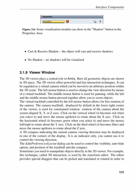
Interface Components
Figure 3.6: Some visualization module can show in the ”Shadow” button in theProperties Area.
• Cast & Receive Shadow – the object will cast and receive shadows
• No Shadow – no shadows will be visualized
3.1.9 Viewer Window
The 3D viewer plays a central role in Amira. Here all geometric objects are shownin 3D space. The 3D viewer offers powerful and fast interaction techniques. It canbe regarded as a virtual camera which can be moved to an arbitrary position withinthe 3D scene. The left mouse button is used to change the view direction by meansof a virtual trackball. The middle mouse button is used for panning, while the leftand the middle mouse button pressed together allow you to zoom objects.The virtual trackball controlled by the left mouse button allows for free rotation ofthe camera. The camera trackball, displayed by default in the lower right cornerof the viewer, is used for constrained rotation: rotation of the camera about thescreen-aligned X, Y, or Z axes. Click on the vertical wheel (it becomes red whenyou select it) and move the mouse up/down to rotate about the X axis. Click onthe horizontal wheel (it becomes green when you select it) and move the mouseleft/right to rotate about the Y axis. Click on the third wheel (it becomes blue) andmove the mouse up/down to rotate about the Z axis.A 3D compass indicating the current camera viewing direction may be displayedin one of the corners of the display. It is an indicator only, you cannot use it tocontrol the viewing direction.The Edit/Preferences/Layout dialog can be used to control the visibility, auto-hideoption, and position of the trackball and the compass.Sometimes you need to manipulate objects directly in the 3D viewer. For example,this technique, called 3D interaction, is used by the transform editor. The editorprovides special draggers that can be picked and translated or rotated in order to
131
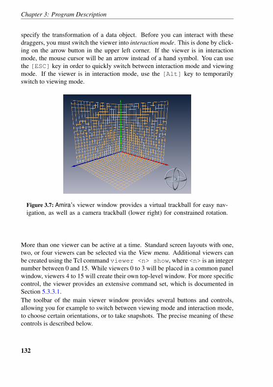
Chapter 3: Program Description
specify the transformation of a data object. Before you can interact with thesedraggers, you must switch the viewer into interaction mode. This is done by click-ing on the arrow button in the upper left corner. If the viewer is in interactionmode, the mouse cursor will be an arrow instead of a hand symbol. You can usethe [ESC] key in order to quickly switch between interaction mode and viewingmode. If the viewer is in interaction mode, use the [Alt] key to temporarilyswitch to viewing mode.
Figure 3.7: Amira’s viewer window provides a virtual trackball for easy nav-igation, as well as a camera trackball (lower right) for constrained rotation.
More than one viewer can be active at a time. Standard screen layouts with one,two, or four viewers can be selected via the View menu. Additional viewers canbe created using the Tcl command viewer <n> show, where <n> is an integernumber between 0 and 15. While viewers 0 to 3 will be placed in a common panelwindow, viewers 4 to 15 will create their own top-level window. For more specificcontrol, the viewer provides an extensive command set, which is documented inSection 5.3.3.1.The toolbar of the main viewer window provides several buttons and controls,allowing you for example to switch between viewing mode and interaction mode,to choose certain orientations, or to take snapshots. The precise meaning of thesecontrols is described below.
132
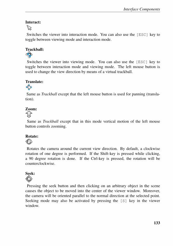
Interface Components
Interact:
Switches the viewer into interaction mode. You can also use the [ESC] key totoggle between viewing mode and interaction mode.
Trackball:
Switches the viewer into viewing mode. You can also use the [ESC] key totoggle between interaction mode and viewing mode. The left mouse button isused to change the view direction by means of a virtual trackball.
Translate:
Same as Trackball except that the left mouse button is used for panning (transla-tion).
Zoom:
Same as Trackball except that in this mode vertical motion of the left mousebutton controls zooming.
Rotate:
Rotates the camera around the current view direction. By default, a clockwiserotation of one degree is performed. If the Shift-key is pressed while clicking,a 90 degree rotation is done. If the Ctrl-key is pressed, the rotation will becounterclockwise.
Seek:
Pressing the seek button and then clicking on an arbitrary object in the scenecauses the object to be moved into the center of the viewer window. Moreover,the camera will be oriented parallel to the normal direction at the selected point.Seeking mode may also be activated by pressing the [S] key in the viewerwindow.
133
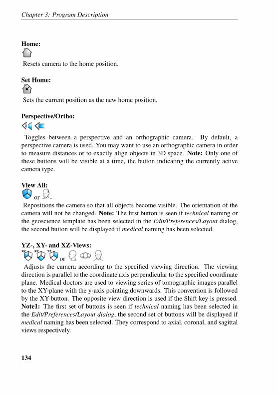
Chapter 3: Program Description
Home:
Resets camera to the home position.
Set Home:
Sets the current position as the new home position.
Perspective/Ortho:
Toggles between a perspective and an orthographic camera. By default, aperspective camera is used. You may want to use an orthographic camera in orderto measure distances or to exactly align objects in 3D space. Note: Only one ofthese buttons will be visible at a time, the button indicating the currently activecamera type.
View All:
orRepositions the camera so that all objects become visible. The orientation of the
camera will not be changed. Note: The first button is seen if technical naming orthe geoscience template has been selected in the Edit/Preferences/Layout dialog,the second button will be displayed if medical naming has been selected.
YZ-, XY- and XZ-Views:
orAdjusts the camera according to the specified viewing direction. The viewing
direction is parallel to the coordinate axis perpendicular to the specified coordinateplane. Medical doctors are used to viewing series of tomographic images parallelto the XY-plane with the y-axis pointing downwards. This convention is followedby the XY-button. The opposite view direction is used if the Shift key is pressed.Note1: The first set of buttons is seen if technical naming has been selected inthe Edit/Preferences/Layout dialog, the second set of buttons will be displayed ifmedical naming has been selected. They correspond to axial, coronal, and sagittalviews respectively.
134
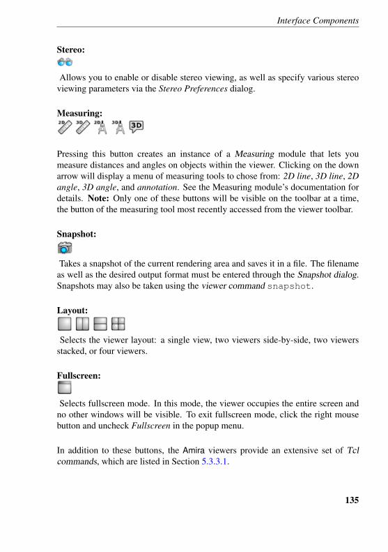
Interface Components
Stereo:
Allows you to enable or disable stereo viewing, as well as specify various stereoviewing parameters via the Stereo Preferences dialog.
Measuring:
Pressing this button creates an instance of a Measuring module that lets youmeasure distances and angles on objects within the viewer. Clicking on the downarrow will display a menu of measuring tools to chose from: 2D line, 3D line, 2Dangle, 3D angle, and annotation. See the Measuring module’s documentation fordetails. Note: Only one of these buttons will be visible on the toolbar at a time,the button of the measuring tool most recently accessed from the viewer toolbar.
Snapshot:
Takes a snapshot of the current rendering area and saves it in a file. The filenameas well as the desired output format must be entered through the Snapshot dialog.Snapshots may also be taken using the viewer command snapshot.
Layout:
Selects the viewer layout: a single view, two viewers side-by-side, two viewersstacked, or four viewers.
Fullscreen:
Selects fullscreen mode. In this mode, the viewer occupies the entire screen andno other windows will be visible. To exit fullscreen mode, click the right mousebutton and uncheck Fullscreen in the popup menu.
In addition to these buttons, the Amira viewers provide an extensive set of Tclcommands, which are listed in Section 5.3.3.1.
135
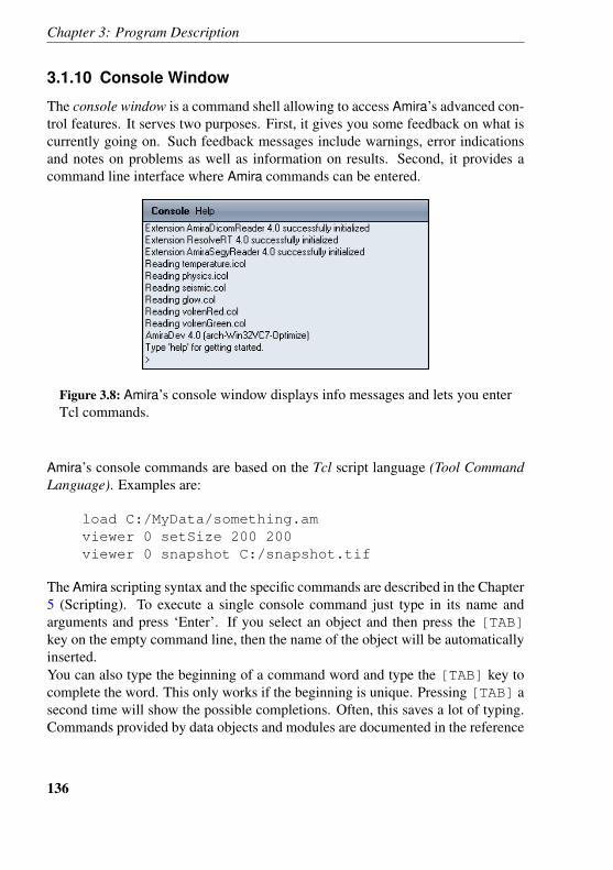
Chapter 3: Program Description
3.1.10 Console Window
The console window is a command shell allowing to access Amira’s advanced con-trol features. It serves two purposes. First, it gives you some feedback on what iscurrently going on. Such feedback messages include warnings, error indicationsand notes on problems as well as information on results. Second, it provides acommand line interface where Amira commands can be entered.
Figure 3.8: Amira’s console window displays info messages and lets you enterTcl commands.
Amira’s console commands are based on the Tcl script language (Tool CommandLanguage). Examples are:
load C:/MyData/something.amviewer 0 setSize 200 200viewer 0 snapshot C:/snapshot.tif
The Amira scripting syntax and the specific commands are described in the Chapter5 (Scripting). To execute a single console command just type in its name andarguments and press ‘Enter’. If you select an object and then press the [TAB]key on the empty command line, then the name of the object will be automaticallyinserted.You can also type the beginning of a command word and type the [TAB] key tocomplete the word. This only works if the beginning is unique. Pressing [TAB] asecond time will show the possible completions. Often, this saves a lot of typing.Commands provided by data objects and modules are documented in the reference
136
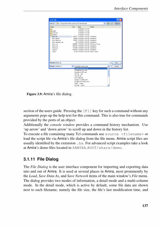
Interface Components
Figure 3.9: Amira’s file dialog.
section of the users guide. Pressing the [F1] key for such a command without anyarguments pops up the help text for this command. This is also true for commandsprovided by the ports of an object.Additionally the console window provides a command history mechanism. Use‘up arrow’ and ‘down arrow’ to scroll up and down in the history list.To execute a file containing many Tcl commands use source <filename> orload the script file via Amira’s file dialog from the file menu. Amira script files areusually identified by the extension .hx. For advanced script examples take a lookat Amira’s demo files located in $AMIRA ROOT/share/demo.
3.1.11 File Dialog
The File Dialog is the user interface component for importing and exporting datainto and out of Amira. It is used at several places in Amira, most prominently bythe Load, Save Data As, and Save Network items of the main window’s File menu.The dialog provides two modes of information, a detail mode and a multi-columnmode. In the detail mode, which is active by default, some file data are shownnext to each filename, namely the file size, the file’s last modification time, and
137
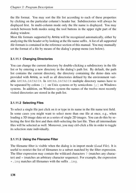
Chapter 3: Program Description
the file format. You may sort the file list according to each of these propertiesby clicking on the particular column’s header bar. Subdirectories will always bedisplayed first. In multi-column mode only the file name is displayed. You mayswitch between both modes using the tool buttons in the upper right part of thedialog window.Most file formats supported by Amira will be recognized automatically, either byanalyzing the file header or by looking at the file name suffix. A list of all supportedfile formats is contained in the reference section of this manual. You may manuallyset the format of a file by means of the dialog’s popup menu (see below).
3.1.11.1 Changing Directories
You can change the current directory by double-clicking a subdirectory in the filelist or by entering a new directory in the dialog’s path list. By default, the pathlist contains the current directory, the directory containing the demo data setsprovided with Amira, as well as all directories defined by the environment vari-able AMIRA DATADIR. In AMIRA DATADIR multiple directory names have tobe separated by colons [:] on Unix systems or by semicolons [;] on Windowssystems. In addition, on Windows system the names of the twelve most recentlyvisited directories are stored in the path list.
3.1.11.2 Selecting Files
To select a single file just click on it or type in its name in the file name text field.In some cases you might want to select more than one file at once, e.g., whenloading a 3D image data set as a series of single 2D images. You can do this by se-lecting the first file first and then shift-selecting the last file. Then all intermediatefiles will be selected as well. Moreover, you may ctrl-click a file in order to toggleits selection state individually.
3.1.11.3 Using the Filename Filter
The filename filter is visible when the dialog is in import mode (Load File). It isuseful to restrict the list of filenames to a subset matched by the filter expression.The filter expression may contain the wildcard characters ? (matches any charac-ter) and * (matches an arbitrary character sequence). For example, the expression*.img matches all filenames with the suffix .img.
138
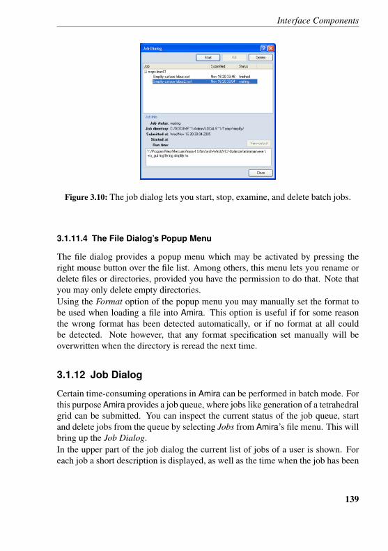
Interface Components
Figure 3.10: The job dialog lets you start, stop, examine, and delete batch jobs.
3.1.11.4 The File Dialog’s Popup Menu
The file dialog provides a popup menu which may be activated by pressing theright mouse button over the file list. Among others, this menu lets you rename ordelete files or directories, provided you have the permission to do that. Note thatyou may only delete empty directories.Using the Format option of the popup menu you may manually set the format tobe used when loading a file into Amira. This option is useful if for some reasonthe wrong format has been detected automatically, or if no format at all couldbe detected. Note however, that any format specification set manually will beoverwritten when the directory is reread the next time.
3.1.12 Job Dialog
Certain time-consuming operations in Amira can be performed in batch mode. Forthis purpose Amira provides a job queue, where jobs like generation of a tetrahedralgrid can be submitted. You can inspect the current status of the job queue, startand delete jobs from the queue by selecting Jobs from Amira’s file menu. This willbring up the Job Dialog.In the upper part of the job dialog the current list of jobs of a user is shown. Foreach job a short description is displayed, as well as the time when the job has been
139
Chapter 3: Program Description
submitted and the current state of the job. A job may be waiting for execution,running, finished, or it may have been killed.
The job directory
For each job a temporary directory is created containing any required input data,scripts, state information, and log files. On Unix systems this directory is createdat the location specified by the environment variable TMPDIR. If no such variableexists, /tmp is used. On Windows systems the default temporary directory isused. Typically this will be C:/TEMP.
Controlling the job queue
A job’s state may be manipulated using the action buttons shown above the joblist. In order to start the job queue select the first job waiting for execution andthen press the Start button. Note that only one job can be executed at a time. Inorder to kill a running job, select it in the job list and press the Kill button. Youmay delete a job from the job queue using the Delete button. When deleting a jobthe temporary job directory will be removed as well.
Information about a job
Once you have selected a job in the job queue, more detailed information about itwill be displayed in the lower part of the dialog window, notably the state of thejob, the temporary job directory, the submit time, the time when the job has beenstarted, the run time, and the name of the command to be executed. Any consoleoutput of a running job will be redirected to a log file located in the temporary jobdirectory. Once such a log file exists and has non-zero size you may inspect it bypushing the View output button.
Commands
job submit cmd info [tmpdir]Submits a new job to the job queue. command specifies the command to beexecuted. info specifies the info string displayed in the job dialog. tmpdirspecifies the temporary job directory. If this argument is omitted a temporaryjob directory is created by Amira itself. In any case, the directory will be auto-matically deleted when the job is removed from the job queue. Example: jobsubmit "clock.exe" "Test job"
140
Interface Components
job run
Starts the first job in job queue pending for execution. When a job is finished,execution of the next job in the queue starts automatically, thus all jobs in thequeue will be executed consecutively by job run.
3.1.13 Preferences Dialog
The Preferences Dialog allows you to adjust certain global settings of Amira. Thepreferences are stored in a permanent fashion on a per-user basis. The dialog con-tains a tab bar with several tabs. The first tab, General, is related to the Pool andsaving the network. The second tab, Layout, affects the layout of the user inter-face. The third, On Exit, controls what conditions are checked for in the networkswhen Amira exits. The Molecules tab allows you to specify options for handlingmolecular data. The LDA tab allows you to specify options for out-of-core data.For advanced users, additional options can be set using the LDAExpertSettingsmodule. The Segmentation tab allows you to specify options for the SegmentationEditor. See the Segmentation Editor documentation for details.
3.1.13.1 The General Tab
2-pass firing algorithmIf set, a slightly more complex firing algorithm is used which ensures that down-
stream modules connected to an up-stream object via multiple paths are only firedonce if the up-stream object changes. The default is on.Auto-select new modulesIf set, a new module selected from the popup menu of its parent object is shown
automatically in the Properties Area. The default is on.Deselect previously selected modulesThis option can only be set if auto-selection is turned on. If set, all objects aredeselected before selecting the new module. Otherwise the new module will beappended at the end of the Properties Area. The default is on.Draw viewer toggles on iconsIf set, small viewer mask toggles are drawn on the icons of data objects and displaymodules. This allows you to show or hide a module in a viewer without selectingit first. The default is on.Draw compute indicatorIf set, a small red rectangle is drawn inside the icon of a module to indicate that
the module is currently working. The default is on.
141
Chapter 3: Program Description
Include unused data objectsIf set, all data objects including hidden colormaps are stored in network scripts.
When executing such a script all existing objects are removed first. If not set onlyvisible data objects and objects which are referenced by others are stored in anetwork script. When executing the script hidden data objects are not removed.The default is on.Include window sizes and positionsIf set, window sizes and positions are stored in network scripts. Be careful usingthis option if you want to send your script to a machine with a different screenresolution.Overwrite existing files in auto-saveIf set, no overwrite check is performed for data objects which need to be saved
automatically in order to create a network script. Otherwise a unique file namewill be chosen. The default is on. Details about the auto-save feature are describedin Section 3.1.1.7.
3.1.13.2 The Layout Tab
Naming conventionThese toggles allow you chose between two naming conventions: medical andtechnical. Your choice will affect the labels of some ports, for example, Orien-tation ports, as well as the appearance of the viewer buttons controlling the vieworientation.WindowsThese items allow you to configure the layout of the Amira windows. By default,the main Amira interface components (Pool, Properties Area, main Viewer win-dow, Console, and Help Browser) share one large window. You can use the checkboxes to display some of these components in separate top-level windows. Thisgives you additional flexibility in managing the ”real-estate” of your graphics dis-play. For example, on a dual-head display it can be interesting to display the mainViewer window on one display and the rest of the Amira interface on the other.Show viewer window in top-level windowThe main Viewer window will be displayed in a top-level window.Show viewer on left-hand sideThe main Viewer window will be displayed on the left-hand side.Show console in top-level windowThe console will be displayed in a top-level window.
142
Interface Components
Show help browser in top-level windowThe help browser will be displayed in a top-level window.Show ”DoIt” buttonsSome modules have a button, usually labeled ”DoIt”, to initiate the action of themodule. Since Amira 4.0, by default, this button is not displayed in the PropertiesArea. Rather, the green Apply button at the bottom of the Properties Area is usedto initiate the action. If this box is checked, the button will be displayed in theProperties Area. The green Apply button will still be available for use as well.Finally, you have the choice to Save current layout (now), and Restore currentlayout (now).Viewer gadgetsThere are two viewer gadgets, a camera trackball and a compass.The camera trackball, used for constrained rotation of the camera about the screen-aligned X, Y, or Z axes, is described in Section 3.1.9.The 3D compass indicates the direction from which the camera is viewing thescene. See Section 3.1.9 for more details on the compass.Click on the tab of the gadget whose attributes you wish to control, then set itsattributes as described below.Show the camera trackballShow the compassThis toggle controls the visibility of the trackball (compass). The default is on.Auto-hide the camera trackballAuto-hide the compassWhen this box is checked, the trackball (compass) is only displayed while themouse is within the trackball (compass) display area. It is hidden as soon as themouse moves outside the trackball (compass) display area. The default is off. Thisitem is not active if the Show the trackball (or compass) item is off.Camera trackball positionCompass positionThis menu allows you to specify which corner of the viewer window to displaythe trackball (compass) in. The default is Lower right for the trackball, and Upperright for the compass. This item is not active if the Show the trackball (or compass)item is off.PoolYou can choose between a graph view and a tree view display of the contents of thePool. The default display modus is the Graph view, which is described in Section3.1.8.1. A description of the Tree view is available in Section 3.1.8.2.
143
Chapter 3: Program Description
If Graph view is selected, you can choose to Show connection ports in the Prop-erties Area. If you check this box on, an object’s/module’s connection ports areshown at the top of its control panel in the Properties Area. By default this is offbecause the connections (shown as blue lines) between data objects and modulescan be conveniently managed directly in the Pool. Changes to the connectionsmade in the Pool are reflected in the connection ports in the Properties Area, andvice versa.If Tree view is selected, this box is always checked on because in tree view, usingthe connection ports in the Properties Area is the only convenient way to managethe connections between data objects and modules.
3.1.13.3 The On Exit Tab
The page allows you to control what conditions are checked for in the networkswhen Amira exits.
3.1.13.4 The Molecules Tab
Color SchemesThese check boxes allow you to chose alternate color schemes: CPK for atoms,and RasMol for amino acids.Selection InfoThese items control how much information is printed into the console when partsof a molecule are selected. Activate Molecule name if the name of the moleculeshould be printed. Activate Group name if the name of the selected group shouldbe printed. If you activate Group attributes, all attributes of the selected group areprinted. If Explicit attributes is activated, the printed attributes are restricted tothose explicitly named in the corresponding text field.Atom Expressions ID case sensitiveSpecifies if atom identifiers are case sensitive or note.
3.1.13.5 The LDA Tab
Out-of-core thresholdSpecifies the size above which data sets will be treated as out-of-core data.CompressionSpecifies the type of data compression.
144
Interface Components
Tile SizeThe size of the tiles to be compressed.Border SizeThe size of border of the tiles.Main memory amountSets the maximum allowed main memory in MB (megabytes) for all the out-of-core data sets.Video memory amountSets the maximum allowed texture memory in MB (megabytes) for all the out-of-core data sets.Viewpoint refinementIf set, refinement depends on the viewpoint.View cullingIf set, refinement takes place only in the view frustum.Move low resolutionIf set, ortho slices and oblique slices are computed in half resolution when moving.Loading policySets loading behavior. If No Interaction is selected, the asynchronous loadingthread will only load when the user does not interact with the scene. If Always isselected, loading occurs as long as there is something to load. If Never is selected,no loading occurs. The default is No Interaction.
3.1.13.6 The Segmentation Tab
3D Draw styleThis option lets you choose the material draw style used in the 3D viewer.Selection Draw styleThis option lets you choose the material draw style used to highlight the voxelsselection.
3.1.13.7 The Rendering Tab
ShadowingIf set, shadows will be generated. You can select also the default behaviour, theintensity and the quality of the shadows. If this option is switched on, some vi-sualization module shows the ”Shadow” button, through which you can directlyspecify the object behaviour.
145
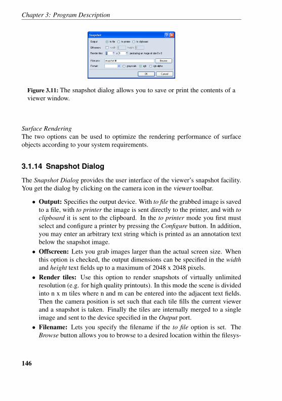
Chapter 3: Program Description
Figure 3.11: The snapshot dialog allows you to save or print the contents of aviewer window.
Surface RenderingThe two options can be used to optimize the rendering performance of surfaceobjects according to your system requirements.
3.1.14 Snapshot Dialog
The Snapshot Dialog provides the user interface of the viewer’s snapshot facility.You get the dialog by clicking on the camera icon in the viewer toolbar.
• Output: Specifies the output device. With to file the grabbed image is savedto a file, with to printer the image is sent directly to the printer, and with toclipboard it is sent to the clipboard. In the to printer mode you first mustselect and configure a printer by pressing the Configure button. In addition,you may enter an arbitrary text string which is printed as an annotation textbelow the snapshot image.
• Offscreen: Lets you grab images larger than the actual screen size. Whenthis option is checked, the output dimensions can be specified in the widthand height text fields up to a maximum of 2048 x 2048 pixels.
• Render tiles: Use this option to render snapshots of virtually unlimitedresolution (e.g. for high quality printouts). In this mode the scene is dividedinto n x m tiles where n and m can be entered into the adjacent text fields.Then the camera position is set such that each tile fills the current viewerand a snapshot is taken. Finally the tiles are internally merged to a singleimage and sent to the device specified in the Output port.
• Filename: Lets you specify the filename if the to file option is set. TheBrowse button allows you to browse to a desired location within the filesys-
146
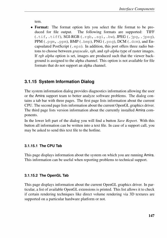
Interface Components
tem.• Format: The format option lets you select the file format to be pro-
duced for file output. The following formats are supported: TIFF(.tif,.tiff), SGI-RGB (.rgb,.sgi,.bw), JPEG (.jpg,.jpeg),PPM (.pgm,.ppm), BMP (.bmp), PNG (.png), DCM (.dcm), and En-capsulated PostScript (.eps). In addition, this port offers three radio but-tons to choose between grayscale, rgb, and rgb alpha type of raster images.If rgb alpha option is set, images are produced such that the viewer back-ground is assigned to the alpha channel. This option is not available for fileformats that do not support an alpha channel.
3.1.15 System Information Dialog
The system information dialog provides diagnostics information allowing the useror the Amira support team to better analyze software problems. The dialog con-tains a tab bar with three pages. The first page lists information about the currentCPU. The second page lists information about the current OpenGL graphics driver.The third page lists version information about the currently installed Amira com-ponents.In the lower left part of the dialog you will find a button Save Report. With thisbutton all information can be written into a text file. In case of a support call, youmay be asked to send this text file to the hotline.
3.1.15.1 The CPU Tab
This page displays information about the system on which you are running Amira.This information can be useful when reporting problems to technical support.
3.1.15.2 The OpenGL Tab
This page displays information about the current OpenGL graphics driver. In par-ticular, a list of available OpenGL extensions is printed. This list allows it to checkif certain rendering techniques like direct volume rendering via 3D textures aresupported on a particular hardware platform or not.
147
Chapter 3: Program Description
3.1.15.3 The Libraries Tab
This page displays a list of all DLLs or shared libraries contained in the Amira libdirectory. For each library certain version information as well as an MD5 check-sum are printed. In this way it is possible to check whether a certain patch hasalready been installed or not. For most libraries the version information is com-piled in. For other libraries this information is read from the version informationfiles found in share/versions in the AMIRA ROOT directory.
3.2 General Concepts
This section contains some general comments on how data objects are organizedand classified in Amira. In particular, the following topics are discussed:
• Amira Class Structure• Scalar and Vector Fields• Coordinates and Grids• Surface Data• Vertex Set• Transformations• Parameters• Shadowing• Subapplication Concept
3.2.1 Class Structure
In this section we discuss the object-oriented design of Amira in a little more detail.You already know that data objects, e.g., gray level image data or vector field sets,appear as separate icons in the Pool. You also know that there are certain displaymodules which can be used to visualize the data objects. While some modules canbe connected to many different data objects, e.g., the Bounding Box module, otherscannot, e.g., the OrthoSlice module. The latter can only be connected to voxeldata or to scalar distributions on voxel grids. The reason is that internally both arerepresented as a scalar field with uniform Cartesian coordinates. Consequently,the same visualization methods can be applied to both. On the other hand, forexample a volumetric tetrahedral grid model of the object of interest usually looks
148
General Concepts
completely different. But since it is also a 3D data object, the same Bounding Boxmodule can be connected to it.In summary, there are Amira data objects that might be conceived of differenttype, but with respect to mathematical structure, applicability of viewing and otherprocessing modules, as well as programming interface design have many com-mon properties. Obeying principles of object-oriented design, the data types ofAmira are organized in class hierarchies where common properties are attributedto ’higher up’ classes and inherited to ’derived’ classes, as sub-classes of a class arecommonly referred to. Conceptually each object occurring in Amira is an instanceof a class and each of its predecessors in the hierarchy that the class belongs to. Theclasses and their hierarchies are defined within Amira. As the user you normallydeal with instances of classes only. For instance, there is a class called ”HxOb-ject” with sub-classes ”HxData” and ”HxModule”. ”HxData” comprises the typesof data associated with data objects used for modeling the objects of interest, e.g.,volumetric tetrahedral grids or surfaces. ”HxModule” comprises data types thathave been assigned to display and other processing modules, again in accordancewith principles of object-oriented design. This is why Amira’s data objects andprocessing modules are commonly referred to as ”objects”.There are also classes in Amira that are not derived from ”HxObject” and constituteother data types, and there are several independent class hierarchies. e.g., there is aclass called ”HxPort” from which all classes supporting the operation and displayof interface control elements are derived (see section Properties Area and the Listof Ports in the index section of the user’s guide).A single class hierarchy is usually figured as an upside-down tree, i.e. with theroot at the top. Thus the data class tree is the one to which the information as towhich processing module is applicable to which data object is hooked. Its classesreflect the mathematical structure of the object models supported by Amira. Forexample, scalar fields and vector fields are such structures and derived from acommon ”field” class which represents a mapping R3→ Rn. Deriving a sub-classfrom this base class requires a value to be specified for n.At the same time fields defined on Cartesian grids are distinguished from fieldsdefined on tetrahedral grids, i.e., this distinction is part of the classification schemethat gives rise to branches in the data class subtree. In the next section of thischapter you will learn more about the data class hierarchy. In the second sectionwe discuss how some data types frequently used for various visualization tasks fitinto it.Internally, all class names begin with a prefix Hx. However, you don’t have toremember these names unless you want to use the command shell to create objects.
149
Chapter 3: Program Description
For example, a bounding box is usually created by choosing the BoundingBox itemfrom the pop-up menu of a data object that is to be visualized, but you may alsocreate it by typing create HxBoundingBox in the command window.
3.2.2 Scalar Field and Vector Fields
The most important fields in Amira are three-dimensional ones. These fields aredefined on a certain domain ⊆ R3. A field can be evaluated at any point inside itsdomain. If the field is defined on a discrete grid, this usually involves some kindof interpolation.
3.2.2.1 Scalar Fields
A 3D scalar field is a mapping R3 → R. The base class of all 3D scalar fields inAmira is HxScalarField3. Various sub-classes represent different ways of defininga scalar field. There are a number of visualization methods for them, for examplepseudo-coloring on cutting planes, iso-surfacing, or volume rendering. However,many visualization modules in Amira rely on a special field representation. There-fore, they can only operate on sub-classes of a general scalar field. Whenever agiven geometry is to be pseudo-colored, any kind of scalar field can be used (cf.Colorwash, GridVolume, Isosurface).The class HxTetraScalarField3 represents a field which is defined on a tetrahedralgrid. On each grid vertex a scalar value, e.g., a temperature, is defined. Valuesassociated to points inside a tetrahedron are obtained from the four vertex valuesby linear interpolation. This class does not provide a copy of the grid itself, insteada reference to the grid is provided. This is indicated in the Pool by a line whichconnects the grid icon and the field icon. As a consequence, a field defined on atetrahedral grid cannot be loaded into the system if the grid itself is not alreadypresent.The class HxRegScalarField3 represents a field which is defined on a regularCartesian grid. Such a grid is organized as a three-dimensional array of nodes.In the most simple case these nodes are axis-aligned and have equal spacings.The coordinates of such a uniform grid can be obtained from a simple bound-ing box containing the origin vector and increments for all directions. Stackedcoordinates are another example. Here the spacing in z-direction between subse-quent slices may be different. In any case scalar values inside a hexahedral gridcell are obtained from the eight vertex values using trilinear interpolation. Whilethe OrthoSlice module can only be used to visualize scalar fields with uniform or
150
General Concepts
stacked coordinates, other modules like ObliqueSlice or Isosurface work for allscalar fields with regular coordinates.Yet another example of a scalar field is the class HxAnnaScalarField3. It representsan analytically defined scalar field. To create such a field, select ScalarField fromthe Create menu of Amira’s main window. You have to specify a mathematicalexpression which is used to evaluate the field at each requested position. Up tothree other fields can be connected to the object. These can be combined to a newscalar field, even if they are defined on different grids.
3.2.2.2 Vector Fields
As for scalar fields Amira provides a number of vector field classes, these are de-rived from the base classes HxVectorField3 and HxComplexVectorField3. Whileordinary vector fields return a three-component vector at each position, complexvector fields return a six-component vector. Complex vector fields are used for en-coding stationary electromagnetic wave pattern as required by some applications.Usually complex vector fields are visualized by projecting them into the space ofreals using different phase offsets. The Vectors module even allows you to animatethe phase offset. In this way a nice impression of the oscillating wave pattern isobtained.
3.2.3 Coordinates and Grids
Amira currently supports two important grid types, namely grids with hexahedralstructure (regular grids), and unstructured tetrahedral grids. Other types, e.g., un-structured grids with hexahedral cells or block-structured grids will be added infuture releases of Amira.
3.2.3.1 Regular Grids
A regular grid consists of a three-dimensional array of nodes. Each node may beaddressed by an index triple (i,j,k). Regular grids are further distinguished accord-ing to the kind of coordinates being used. The most simple case comprises uniformcoordinates, where all cells are assumed to be rectangular and axis-aligned. More-over, the grid spacing is constant along each axis. A grid with stacked coordinatesmay be imagined as a stack of uniform 2D slices. However, the distance betweenneighboring slices in z-direction may vary. In case of rectilinear coordinates thecells are still aligned to the axes, but the grid spacing may vary from cell to cell.
151
Chapter 3: Program Description
Finally, in case of curvilinear coordinates each node of the grid may have arbitrarycoordinates. Grids with curvilinear coordinates are often used in fluid dynamicsbecause they have a simple structure but still allow for accurate modeling of com-plex shapes like rotor blades or airfoils.
3.2.3.2 Tetrahedral Grids
The TetraGrid class represents a volumetric grid composed of many tetrahedrons.Such grids can generally be used to perform finite-element simulations, e.g., E-field simulations.A considerable amount of information is maintained in a TetraGrid. For eachvertex a 3D coordinate vector is stored. For each tetrahedron the indices of itsfour vertices are stored as well as a number indicating the segment the tetrahedronbelongs to as obtained by a segmentation procedure. Beside this fundamental in-formation a number of additional variables are stored in order for the grid beingdisplayed quickly. In particular all triangles or faces are stored separately togetherwith six face indices for each tetrahedron. In addition for each face pointers to thetwo tetrahedrons it belongs to are stored. This way the neighborhood informationcan be obtained efficiently.When simulating E-fields using the finite-element method, the edges of a grid needto be stored explicitly, because vector or Whitney elements are used. These ele-ments and its corresponding coefficients are defined on a per-edge basis. When agrid is selected information on the number of its vertices, edges, faces, and tetra-hedrons is displayed.
3.2.4 Surface Data
Amira provides a special-purpose data class for representing triangular surfaces,called HxSurface. This class is documented in more detail in the index section ofthe user’s guide. For the moment, we only mention that the class maintains con-nectivity information and that it may represent manifold as well as non-manifoldtopologies.The surface class provides a rich set of Tcl commands. It is a good example of anAmira data class that does not simply store information, but allows the user to queryand manipulate the data by means of special-purpose methods and interfaces.
152
General Concepts
3.2.5 Vertex Set
Another example of data abstraction and inheritance is the VertexSet class. Manydata objects in Amira are derived from this class, e.g., landmark sets, molecules,surfaces, or tetrahedral grids. All these objects provide a list of points with x-, y-,and z-coordinates. Other modules which require a list of points as input only needto access the VertexSet base class, but don’t need to know the actual type of thedata object.
One such example of a generic module operating on VertexSet objects is the Ver-texView module. This module allows you to visualize vertex positions by drawingdots or little spheres at each point.
3.2.6 Transformations
Data objects in Amira can be modified using an arbitrary affine transformation.For example, this makes it possible to align two different data objects so that theyroughly match each other. Internally, affine transformations are represented by a4x4 transformation matrix. In particular, a uniform scalar field remains a uniformscalar field, even if it is rotated or sheared. Display modules like OrthoSlice stillcan exploit the simple structure of the uniform field. The possible transformationis automatically applied to any geometry shown in the 3D viewer.
In order to interactively manipulate the transformation matrix use the TransformEditor (documentation is contained in the index section of the user’s guide).
Be careful when saving transformed data sets! Most file formats do not allow tostore affine transformations. In this case you have to apply the current transforma-tion to the data. This can be done using the Tcl-command applyTransform.In case of vertex set objects the transformation is applied to all vertices. Old coor-dinates are replaced by new ones, and the transformation matrix is reset to identityafterwards. After a transformation has been applied to a data set, it cannot be unseteasily anymore.
If a transformation is applied to uniform fields, e.g., to 3D image data, the coor-dinate structure is not changed, i.e., the field remains a uniform one. Instead, thedata values are resampled, i.e., the transformed field is evaluated at every vertex ofthe final regular grid. The bounding box of the resulting grid is modified so that itcompletely encloses the transformed original box.
153
Chapter 3: Program Description
3.2.7 Parameters
For any data object an arbitrary number of additional parameters or attributes maybe defined. Parameters can be interactively added, deleted, or edited using theparameter editor. Parameters are useful for example to store certain parameters ofa simulation or of an experiment. In this way the history of a data object can befollowed.There are certain parameters which are interpreted by several Amira modules. Themeaning of these parameters is summarized in the following list:
• Colormap nameThis specifies the name of the default colormap used to visualize the data.Some modules automatically search the Pool for this colormap and for ex-ample use it for pseudocoloring.
• DataWindow minVal maxValThis indicates the preferred data range used for visualizing the data. TheOrthoSlice module automatically maps values below minVal to black andvalues above maxVal to white.
• LoadCmd cmdThis parameter is usually set by import filters when a data object is read. Itis used when saving the current network into a file and it allows to restorethe object automatically. Internal use only.
Note that there are many file formats which do not allow to store parameters.Therefore, information might get lost when you save the data set in such a for-mat. If in doubt, use the Amira specific AmiraMesh format.
3.2.8 Shadowing
Real time shadow casting is enabled through the Edit/Preferences/Renderingmenu.Once enabled, most of display modules can cast or receive shadows.Different modes are available, and switching from one to another is possible byclicking on the shadow icon of a display module
• No Shadows the displayed shape neither cast or receive shadows
• Cast Shadows the displayed shape only cast shadows
• Receive shadows the displayed shape only receive shadows
154
General Concepts
• Cast & Receive shadows the displayed shape both cast and receive
shadows
Restrictions:
At least the Multi-Texture and Texture Environment Combine OpenGL extensionsmust be supported by your graphics board. Otherwise no shadows will becomputed. These extensions are now standard in OpenGL 1.3 and later.
The Shadow and Depth Texture OpenGL extensions (standard in OpenGL 1.4)are used if they are available and generally improve performance.
Some aliasing artifacts can appear if you zoom in very close to the scene. You canthen increase the quality in the preferences dialog.
Transparent objects are treated as follows, depending on the transparency type:
• Screen door: fully compatible• Add, Blend : transparent objects cast a shadow and are shadowed but
the shadow intensity doesn’t depend on the transparency value (the sameshadow is displayed for full transparent shapes and opaque shapes).
• All other modes : incompatible with shadowing.
3.2.9 Sub-application Concept
Beside visualization modules, the user interface enable an easier and faster swapbetween application areas. With the user-friendly ”sub-application” concept sev-eral dedicated components are accessible as independent applications assembledtogether into the general Amira platform. Each component provides its own spe-cific interface, its dedicated tools and visualization options. Since switching be-tween different components takes place through a simple toolbar, the user can ex-plore and approach complex data sets using dedicated tools in the sub-applications,and keep a clear overview in the general purpose framework. To access the sub-application a toolbar is available in the upper-left corner of the main window.The following components are currently sub-applications:
• Object Pool
155
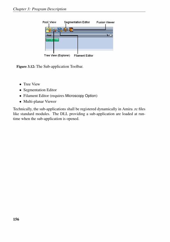
Chapter 3: Program Description
Figure 3.12: The Sub-application Toolbar.
• Tree View• Segmentation Editor• Filament Editor (requires Microscopy Option)• Multi-planar Viewer
Technically, the sub-applications shall be registered dynamically in Amira .rc fileslike standard modules. The DLL providing a sub-application are loaded at run-time when the sub-application is opened.
156
4 Technical Information
This chapter contains technical information about Amira which is not covered inthe previous chapters.
• Data Import• Command Line Options• Environment Variables• Amira start-up script• System Requirements• Amira License Manager• Notes for Mac users
4.1 Data Import
Usually, one of the first things Amira users want to know is how to import theirown data into the system. This section contains some advice intended to ease thistask.In the simplest case, your data is already present in a standard file format supportedby Amira. To import such files, simply use the File Load menu. A list of allsupported formats can be found in the index section of the user’s guide. Usually,the system recognizes the format of a file automatically by analyzing the file headeror the filename suffix. If a supported format is detected, the file browser indicatesthe format name.Often, 3D image volumes are stored slice by slice using standard 2D image formatssuch as TIFF or JPEG. In case of medical images, slices are commonly stored inACR-NEMA or DICOM format. If you select multiple 2D slices simultaneouslyin the file browser, all slices will automatically be combined into a single 3D dataset. Simultaneous selection is most easily achieved by first clicking the first sliceand then shift-clicking the last one.If your data is not already present in a standard file format supported by Amira youwill have to write your own converter or export filter. For many data objects such
157
Chapter 4: Technical Information
as 3D images, regular fields, or tetrahedral grids Amira’s native AmiraMesh formatis most appropriate. Using this format you can even represent point sets or linesegments for which there is hardly any other standard format. The AmiraMeshdocumentation explains the file syntax in detail and contains examples of howto encode different data objects. One important Amira data type, triangular non-manifold surfaces, cannot be represented in a AmiraMesh file but has its own fileformat called HxSurface format.Alternatively, with Developer Option a C++ programmer can extend Amira in orderto integrate a custom reader or writer.Finally, in case of images or regular fields with uniform coordinates you may alsoread binary raw data. Note that for raw data the dimensions and the bounding boxof the data volume must be entered manually in a dialog box which pops up afteryou have selected the file in the file browser.
4.2 Command Line Options
This section describes the command line options understood by Amira. In general,on Unix systems Amira is started via the start script located in the subdirec-tory bin. Usually, this script will be linked to /usr/local/bin/Amira orsomething similar. Alternatively, the user may define an alias Amira pointing tobin/start.On Windows systems Amira is usually started via the start menu or via a desktopicon. Nevertheless, the Amira executable may also be invoked directly by callingbin/arch-Win32VC8-Optimize/Amiramain.exe. In this case, the samecommand line options as on a Unix system are understood.The syntax of Amira is as follows:
Amira [options] [files ...]
Data files specified in the command line will be loaded automatically. In additionto data files, script files can also be specified. These scripts will be executed whenthe program starts.The following options are supported:
• -helpPrints a short summary of command line options.
• -versionPrints the version string of Amira.
158
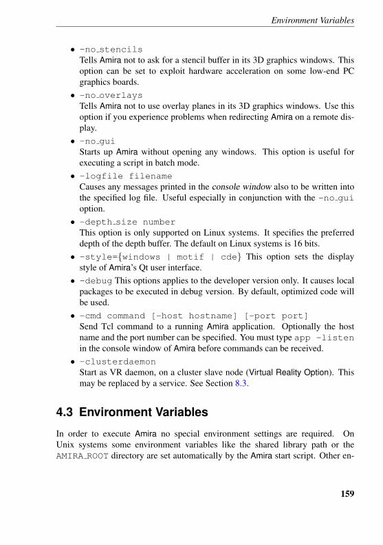
Environment Variables
• -no stencilsTells Amira not to ask for a stencil buffer in its 3D graphics windows. Thisoption can be set to exploit hardware acceleration on some low-end PCgraphics boards.
• -no overlaysTells Amira not to use overlay planes in its 3D graphics windows. Use thisoption if you experience problems when redirecting Amira on a remote dis-play.
• -no guiStarts up Amira without opening any windows. This option is useful forexecuting a script in batch mode.
• -logfile filenameCauses any messages printed in the console window also to be written intothe specified log file. Useful especially in conjunction with the -no guioption.
• -depth size numberThis option is only supported on Linux systems. It specifies the preferreddepth of the depth buffer. The default on Linux systems is 16 bits.
• -style={windows | motif | cde} This option sets the displaystyle of Amira’s Qt user interface.
• -debug This options applies to the developer version only. It causes localpackages to be executed in debug version. By default, optimized code willbe used.
• -cmd command [-host hostname] [-port port]Send Tcl command to a running Amira application. Optionally the hostname and the port number can be specified. You must type app -listenin the console window of Amira before commands can be received.
• -clusterdaemonStart as VR daemon, on a cluster slave node (Virtual Reality Option). Thismay be replaced by a service. See Section 8.3.
4.3 Environment Variables
In order to execute Amira no special environment settings are required. OnUnix systems some environment variables like the shared library path or theAMIRA ROOT directory are set automatically by the Amira start script. Other en-
159
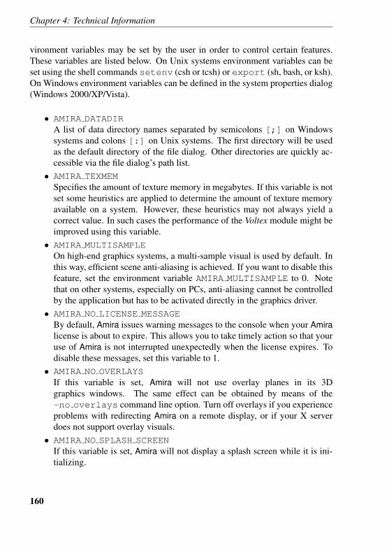
Chapter 4: Technical Information
vironment variables may be set by the user in order to control certain features.These variables are listed below. On Unix systems environment variables can beset using the shell commands setenv (csh or tcsh) or export (sh, bash, or ksh).On Windows environment variables can be defined in the system properties dialog(Windows 2000/XP/Vista).
• AMIRA DATADIRA list of data directory names separated by semicolons [;] on Windowssystems and colons [:] on Unix systems. The first directory will be usedas the default directory of the file dialog. Other directories are quickly ac-cessible via the file dialog’s path list.
• AMIRA TEXMEMSpecifies the amount of texture memory in megabytes. If this variable is notset some heuristics are applied to determine the amount of texture memoryavailable on a system. However, these heuristics may not always yield acorrect value. In such cases the performance of the Voltex module might beimproved using this variable.
• AMIRA MULTISAMPLEOn high-end graphics systems, a multi-sample visual is used by default. Inthis way, efficient scene anti-aliasing is achieved. If you want to disable thisfeature, set the environment variable AMIRA MULTISAMPLE to 0. Notethat on other systems, especially on PCs, anti-aliasing cannot be controlledby the application but has to be activated directly in the graphics driver.
• AMIRA NO LICENSE MESSAGEBy default, Amira issues warning messages to the console when your Amiralicense is about to expire. This allows you to take timely action so that youruse of Amira is not interrupted unexpectedly when the license expires. Todisable these messages, set this variable to 1.
• AMIRA NO OVERLAYSIf this variable is set, Amira will not use overlay planes in its 3Dgraphics windows. The same effect can be obtained by means of the-no overlays command line option. Turn off overlays if you experienceproblems with redirecting Amira on a remote display, or if your X serverdoes not support overlay visuals.
• AMIRA NO SPLASH SCREENIf this variable is set, Amira will not display a splash screen while it is ini-tializing.
160
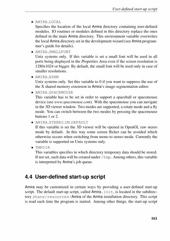
User-defined start-up script
• AMIRA LOCALSpecifies the location of the local Amira directory containing user-definedmodules. IO routines or modules defined in this directory replace the onesdefined in the main Amira directory. This environment variable overwritesthe local Amira directory set in the development wizard (see Amira program-mer’s guide for details).• AMIRA SMALLFONT
Unix systems only. If this variable is set a small font will be used in allports being displayed in the Properties Area even if the screen resolution is1280x1024 or bigger. By default, the small font will be used only in case ofsmaller resolutions.
• AMIRA XSHMUnix systems only. Set this variable to 0 if you want to suppress the use ofthe X shared memory extension in Amira’s image segmentation editor.
• AMIRA SPACEMOUSEThis variable has to be set in order to support a spaceball or spacemousedevice (see www.spacemouse.com). With the spacemouse you can navigatein the 3D viewer window. Two modes are supported, a rotate mode and a flymode. You can switch between the two modes by pressing the spacemousebuttons 1 or 2.
• AMIRA STEREO ON DEFAULTIf this variable is set the 3D viewer will be opened in OpenGL raw stereomode by default. In this way some screen flicker can be avoided whichotherwise occurs when switching from mono to stereo mode. Currently thevariable is supported on Unix systems only.
• TMPDIRThis variables specifies in which directory temporary data should be stored.If not set, such data will be created under /tmp. Among others, this variableis interpreted by Amira’s job queue.
4.4 User-defined start-up script
Amira may be customized in certain ways by providing a user-defined start-upscript. The default start-up script, called Amira.init, is located in the subdirec-tory share/resources/Amira of the Amira installation directory. This scriptis read each time the program is started. Among other things, the start-up script
161
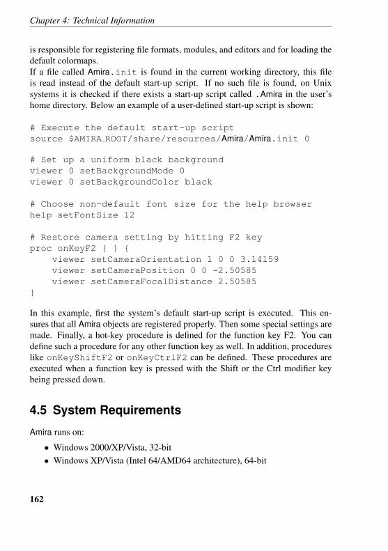
Chapter 4: Technical Information
is responsible for registering file formats, modules, and editors and for loading thedefault colormaps.If a file called Amira.init is found in the current working directory, this fileis read instead of the default start-up script. If no such file is found, on Unixsystems it is checked if there exists a start-up script called .Amira in the user’shome directory. Below an example of a user-defined start-up script is shown:
# Execute the default start-up scriptsource $AMIRA ROOT/share/resources/Amira/Amira.init 0
# Set up a uniform black backgroundviewer 0 setBackgroundMode 0viewer 0 setBackgroundColor black
# Choose non-default font size for the help browserhelp setFontSize 12
# Restore camera setting by hitting F2 keyproc onKeyF2 { } {
viewer setCameraOrientation 1 0 0 3.14159viewer setCameraPosition 0 0 -2.50585viewer setCameraFocalDistance 2.50585
}
In this example, first the system’s default start-up script is executed. This en-sures that all Amira objects are registered properly. Then some special settings aremade. Finally, a hot-key procedure is defined for the function key F2. You candefine such a procedure for any other function key as well. In addition, procedureslike onKeyShiftF2 or onKeyCtrlF2 can be defined. These procedures areexecuted when a function key is pressed with the Shift or the Ctrl modifier keybeing pressed down.
4.5 System Requirements
Amira runs on:
• Windows 2000/XP/Vista, 32-bit• Windows XP/Vista (Intel 64/AMD64 architecture), 64-bit
162

System Requirements
• Mac OS X 10.5 (Leopard) with Intel CPU• Red Hat Enterprise Linux 5.0 for x86 64 or compatible
Amira relies on hardware-accelerated OpenGL 3D graphics. Please note that ifsoftware rendering is used, rendering performance may drop significantly, espe-cially for visualization techniques like volume rendering. Some visualization tech-niques may also require 3D texturing or programmable shaders, available on recentgraphics boards. For platform-specific details on hardware acceleration, see below.Amira requires a display resolution of at least 1024x768 and at least 15 bits ofcolor depth. We strongly recommend 1280x1024 with 24-bit color depth at least.
Apart from 3D graphics hardware, probably the most important system parameteris main memory. You should have at least 512 MB, preferably 2 GB or more.The speed of the processor of course is also an important parameter. However itis less critical than the graphics system and the main memory size. For the PCversions, we recommend at least a 2 GHz processor.
4.5.1 Troubleshooting
Amira is a very demanding application that extensively uses high-end features. Ex-perience shows that such applications tend to reveal instabilities in system hard-ware, hardware drivers, and the operating system. A common problem is insuf-ficient main memory. We recommend you configure enough swap memory inaddition to physical memory. The total amount of virtual memory should be atleast 1 GB. 2 GB would be even better.Especially on PC platforms, OpenGL drivers today are not always as robust as de-sired. Also, system crashes due to bad memory chips or unstable power-supply arenot rare. If you experience problems or instabilities with Amira on your Windowsplatform, we recommend that you follow these steps:
1. Click on all the demo scripts in the Online User’s Guide. If the systemcrashes, turn off hardware acceleration (choose the extended button fromthe Windows display settings dialog) and try again. If this eliminates theproblem, there is a bug in your OpenGL driver. Try to get a new driver fromthe web site of the manufacturer of your graphics board.
2. Try using a different color depth in the Windows display settings dialog. Try24 or 32 bit.
163
Chapter 4: Technical Information
3. Load the lobus.am data set and visualize it with a Voltex module. Turn onthe spin rotation (turn it with the mouse in the viewer and release the mousebutton while moving the mouse, so that the object continues moving). Let itrun overnight (turn off the screen saver). If the system has crashed or frozenthe next morning, you probably have a hardware problem.
If this does not help, or if a reproducible error occurs on different computers, thenit might be a bug in the Amira software itself. Please report such bugs so that theycan be eliminated in the next release or a patch can be prepared.
4.5.2 Microsoft Windows
Amira runs on Intel or AMD-based systems with Microsoft Windows 2000, Mi-crosoft Windows XP and Microsoft Windows Vista, 32 bits and 64 bits.Graphics Hardware: You should use a graphics board with OpenGL support andtexture mapping capabilities. Some visualization techniques may also require 3Dtexturing and programmable shaders, available on recent graphics boards.Note: On Windows Vista, you may want to disable Windows Aero for savinghardware resources and achieving best 3D performance with Amira. In ControlPanel, open Appearance and Personalization, then click Personalization. You canalternatively right-click an empty spot on your desktop and click Personalize inpop-up. Click Window Color and Appearance, and then click Open Classic Ap-pearance Properties for More Color Options. Now you can select a Color schemedifferent from Windows Aero, such as the Windows classic theme.In order to add custom extensions to Amira with Developer Option you will needVisual Studio 2005, while Visual Studio 2008 is not officially supported for devel-opment. Even though not supported, you may compile new modules with VisualStudio 2008, but you will need to install the Visual Studio 2008 C runtimes addi-tionally to Amira on any Windows PC that uses your custom modules.
4.5.3 Linux
The Linux version of Amira as been developed and tested on Red Hat EnterpriseLinux 4.0 and 5.0.On other Linux distributions this version might not run because certain requiredsystem libraries are missing or because different versions of these libraries areinstalled. In particular you may need to install libstdc++.so.5 included in the
164
System Requirements
compat-libstdc++ package (or you may copy it into the Amira installation directoryunder lib/arch-Linux...-Optimize/).
On Linux, Amira is only available for AMD64 / Intel 64 systems.
Graphics Hardware: Amira works with the current 3D graphics drivers fromnVidia and ATI under XFree86 4/Xorg.
Notes:
• After a standard installation of Linux, hardware acceleration is not neces-sarily activated, although X-Windows and Amira may work fine. To enableOpenGL hardware acceleration specific drivers may have to be installed.This can dramatically increase rendering performance. Sometimes it isnecessary to disable the stencil buffers (by starting Amira with the option-no stencils) to get acceleration.
• On some distribution, you may see incorrect display of some parts ofthe user interface, such as the segmentation editor. This is a known Qtissue. You can work around this by disabling the composite option in theextension section of your XFree86.conf or Xorg.conf configuration file:
Section "Extensions"Option "Composite" "disable"
EndSection
In order to add custom extensions to Amira with Developer Option you will needgcc 4.1.x on RHEL 5.
4.5.4 Mac OS
The Mac version of Amira has been developed and tested on Mac OS X 10.5 (Leop-ard) running on an Intel CPU. This version might not work properly on other MacOS releases or non-Intel CPU Apple platforms.
In order to add custom extensions to Amira with Developer Option you will needgcc 4.0.x provided by the standard XCode development environment.
Graphics Hardware: Amira works with the current Mac 3D graphics drivers fromnVidia and ATI.
165
Chapter 4: Technical Information
4.6 Amira License Manager
4.6.1 Contents
• About Password Protection• About the Amira License Manager• Troubleshooting• Using TGS LICENSE DEBUG• Contacting the License Administrator• Contacting Technical Support
4.6.2 About Password Protection
Your Amira software is ”password enabled”. Each time the software runs, itchecks for a valid password. If a valid password is found, the application runs.Otherwise, a license dialog is displayed, allowing you to enter a valid Amiralicense.
Generally, your software is also ”computer ID locked”. Computer ID lock-ing is a form of software license control that allows the software to run onlyon specifically licensed systems. If your license is for a specific system, yourpassword string will include a computer ID.
If your site has purchased Amira floating licenses for use with FLEXNet, you willfind information in a specific section about Configuring FLEXNet Licensing, in-cluding instructions for installing the Client License Files. This documentationmay be found in
<install directory>/share/license/FLEXNet
4.6.3 About the Amira License Manager
The Amira License Manager dialog is displayed when you attempt to start Amiraon a system for which no valid Amira license is found:
The Amira License Manager has an editable text field displaying the contents ofthe active license file. The path of the active license file is given in the box above.
166
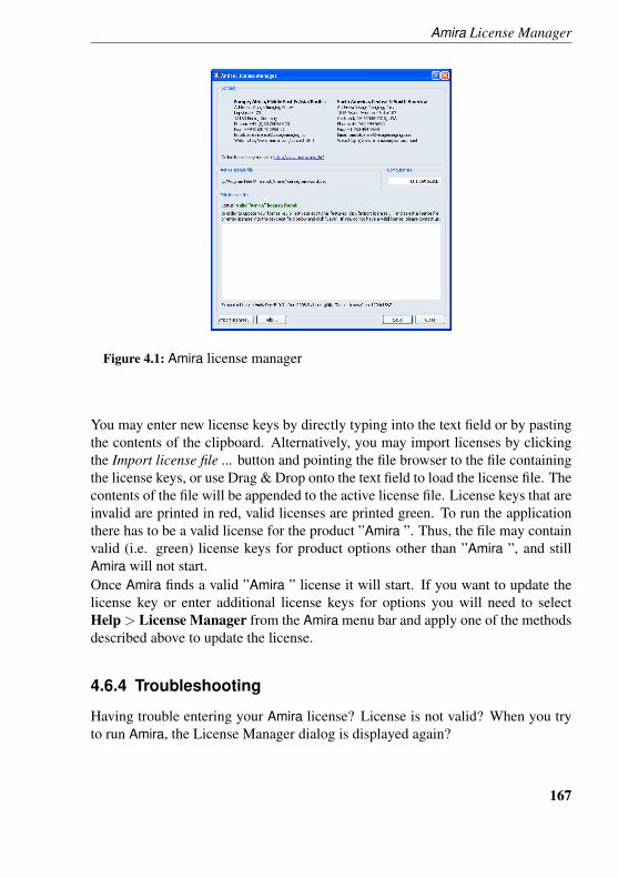
Amira License Manager
Figure 4.1: Amira license manager
You may enter new license keys by directly typing into the text field or by pastingthe contents of the clipboard. Alternatively, you may import licenses by clickingthe Import license file ... button and pointing the file browser to the file containingthe license keys, or use Drag & Drop onto the text field to load the license file. Thecontents of the file will be appended to the active license file. License keys that areinvalid are printed in red, valid licenses are printed green. To run the applicationthere has to be a valid license for the product ”Amira ”. Thus, the file may containvalid (i.e. green) license keys for product options other than ”Amira ”, and stillAmira will not start.Once Amira finds a valid ”Amira ” license it will start. If you want to update thelicense key or enter additional license keys for options you will need to selectHelp > License Manager from the Amira menu bar and apply one of the methodsdescribed above to update the license.
4.6.4 Troubleshooting
Having trouble entering your Amira license? License is not valid? When you tryto run Amira, the License Manager dialog is displayed again?
167
Chapter 4: Technical Information
Here are steps for remedying the situation.
1. If you are using an evaluation or demo license,
License Amira 5.0 31-Oct-2006 0 7f3a8i5u4j4j"Demo License"
make sure that expiration date is in the future.Action: Ask your Amira reseller for an extension of the trial period orpurchase a license.
2. If your license key has a computer ID, for example,
License Amira 5.0 31-Oct-2006 0 7f3a8i5u4j4j"JustTesting" 001422505396
make sure that the computer ID of your license key matches the computerID shown in the computer ID field of the License Manager.Action: If the computer IDs do not match, you will need to request a newlicense from the License Administrator (see below). Please supply the hostID from the License Manager dialog as well as your existing license key forreference.
3. If the above suggestions do not resolve the license problem, itwill be necessary to debug the problem using environment variableTGS LICENSE DEBUG. See below for instructions.
4.6.5 Using TGS LICENSE DEBUG
If the TGS LICENSE DEBUG environment variable is set to a file name, whenAmira is run, licensing debug output is written to the specified file. You can open
168

Amira License Manager
and read this debug file yourself. However, most likely you will need to send it tothe technical support team (see below) for analysis.Below are instructions for setting this environment variable on Windows and onLinux/UNIX systems.
4.6.5.1 Windows
On Windows, you can set the environment variable via the Control Panel or youcan set it in a command prompt.Windows - Control Panel
1. You can get to the Control Panel via the Windows Start menu.2. In the Control Panel, select the System application.3. Click on the Advanced tab.4. Press the Environment variables button.5. In either the User or System variables, press the New button.6. For the Variable name enter TGS LICENSE DEBUG.7. For the Variable value enter ”debug.txt” (without the quotes).8. Click all of the OK buttons to exit the dialog.9. Run Amira from the Start menu. When the License Manager dialog comes
up, dismiss it.10. Then look for a file named ”debug.txt” in the top level of the Amira installa-
tion directory. Send that file to tech support for analysis.
Windows - Command Prompt
1. On Windows 2000 and Windows XP you can get to a command prompt viathe Windows Start menu as follows: Start > Programs > Accessories >Command Prompt
2. In the command prompt window, type:set TGS LICENSE DEBUG=debug.txt
3. Change the current directory to where your Amira executable is. For exam-ple,cd /Program Files/Amira5/bin/arch-Win32VC8-Optimize
4. Run Amira as follows:Amiramain.exe
5. When the License Manager dialog comes up, dismiss it.
169

Chapter 4: Technical Information
6. Look for the file debug.txt in the current directory. Send that file to techsupport for analysis.
4.6.5.2 On Linux/UNIX
1. On Linux/UNIX systems, the exact command to use for setting environmentvariables depends on the kind of shell you are using. Here are examples fora few commonly used shells. Bash shell:export TGS LICENSE DEBUG=debug.txt C shell:setenv TGS LICENSE DEBUG debug.txt
2. In the window in which you set the environment variable, cd to the directorycontaining the Amira executable. For example,
cd /opt/Amira5
3. Run Amira as follows:
bin/start
4. When the License Manager dialog comes up, dismiss it.5. Look for the file debug.txt in the current directory. Send that file to tech
support for analysis.NOTE: If you don’t see the debug.txt file there, possibly you do not haveprivilege to write into the Amira installation directory. In this case, setTGS LICENSE DEBUG to a path where you can write. For example,/home/your login name/debug.txt
4.6.6 Contacting the License Administrator
From North, South, and Central [email protected] Europe, Middle East, Africa, Asia, and [email protected]
4.6.7 Contacting Technical Support
From North, South, and Central [email protected]
170
Notes for Mac users
From Europe, Middle East, Africa, Asia, and [email protected]
4.7 Notes for Mac users
The user will find several important differences when comparing the Mac to theWindows version. Due to the platform architecture, the Mac version requires spe-cific implementation not only for the interface components, but also for the mod-ules functionalities. Additionally, the tutorials have been developed on Windowsplatforms. Therefore, the user has to keep in mind the following issues when read-ing the examples of the tutorials and whenever using Amira:
• Ctrl Key - The Ctrl key of Windows and Linux corresponds to the Ap-ple/Command key on Mac platforms.
• Stereo - Stereo visualization is not fully supported on Mac, due to OpenInventor compatibilities. Only few stereo modes are, therefore, available.
• Main Menu - The main menu on Mac has been redesigned according to thenative style. The first item in the main menu is application item ”Amira”,where application-specific information are available as About Amira or Pref-erences....
• Graphic performances - High-end graphic boards are required to use the Vol-ren module and the editors using this visualization technique. Some iMacand older Mac platforms may not have adequate graphic cards.
• amiraDev - After developing new modules using the amiraDev Package,start Amira normally to use or test them. Starting Amira in ”debug mode”is not required for Mac platforms. See the amiraDev documentation fordetails.
4.8 Amira and the /3GB switch
This page describes problems and possible solutions related to the usage of largedata sets in Amira 5 on computers running Windows XP. If you frequently en-counter dialogs in Amira such as ”cannot allocate xxxxxx bytes of memory” al-though you think you have enough physical memory installed, then the informa-tion provided on this page might be useful for you.
171
Chapter 4: Technical Information
4.8.1 The Problem
Any 32-bit operating system such as Windows (NT4.0, 2000, XP) or Linux canmanage at most 4 gigabytes (GB) of memory. Windows divides this addressablespace into 2 GB reserved for usage by the system only and 2 GB for any userapplication. Therefore, a single application can use at maximum 2 GB of memory.Note that this is independent of the actual physical memory, i.e., it does not matterwhether the system has 1, 2, 3 or 4 GB of memory installed. Within the 2 GBreserved for the user, the software itself (executable and all of its DLLs) and all ofthe data has to fit. This makes clear that it is impossible for a Windows programto load 2 GB of data at a time.To overcome this, Microsoft has provided a boot option for Windows that alterspartitioning of address space so that 3 GB are reserved for the user and 1 GB forthe system. This boot option is available starting with Windows XP Service Pack2.
4.8.2 How to activate the /3GB switch
It should be noted that we cannot guarantee that the following changes to be madein your system will not affect the execution of other programs although we havenot found any incompatibilities so far. We also wish to stress that we assume noresponsibility for any loss of data as a consequence of those changes. We thereforestrongly recommend that you back up your system before making these changes.All you need to do is to edit the file C:/boot.ini. To do so, make sure that youare logged on your machine with administrative privileges. Then select fromStart->Settings->Control Panel->System->Advanced->(Startup and Recovery)Settings and click the Edit button. Duplicate the line under [operating systems].Change the name between the quotes and add the ”/3GB” switch right after the”/fastdetect” switch. The new entry might look then similar to this:
[operating systems]multi(0)disk(0)rdisk(0)partition(1)\WINDOWS="Microsoft Windows XP \
Professional" /fastdetectmulti(0)disk(0)rdisk(0)partition(1)\WINDOWS="Microsoft Windows XP \
Professional 3GB" /fastdetect /3GB
Note that for the usage of the /3GB boot option the application must be aware ofthe altered memory assignment. For Amira 5 there is already native support forthe /3GB boot option. If you are using an older version of Amira, we stronglyrecommend updating to 5.
172
Amira and the /3GB switch
Now, as you boot up your computer, a screen is displayed that gives you the choicebetween two boot options. Use the arrow keys to select the entry with the ”3GB”in the line and press return. Amira should now be able to address 3 GB of memoryinstead of the default 2 GB. You can appreciate this by comparing the result of”app maxmalloc” in the Amira console window with and without the 3 GB option.On a typical installation with 1 GB of memory installed and without the /3GBswitch, the command ”app maxmalloc” may result in something like this:
Allocated chunk of 942 MB.Allocated chunk of 225 MB.Allocated chunk of 129 MB.Allocated chunk of 121 MB.Allocated chunk of 72 MB.Allocated a total of 1723 MB in 25 chunks
With the /3GB switch on the same installation, the command results in the follow-ing:
Allocated chunk of 1023 MB.Allocated chunk of 919 MB.Allocated chunk of 225 MB.Allocated chunk of 111 MB.Allocated a total of 2278 MB in 4 chunks
What you can see is that the total amount of allocatable memory has not changeddramatically. However, with the /3GB switch, the second largest chunk of memoryis nearly as large as the first one.
173

5 Scripting
5.1 Introduction
This chapter is intended for advanced Amira users only. If you do not know whatscripting is, it is very likely that you will not need the features described in thischapter.Beside the interactive control via the graphical user interface, most of the Amirafunctionality can also be accessed using specific commands. This allows you toautomate certain processes and to create scripts for managing routine tasks or forpresenting demos. Amira’s scripting commands are based on Tcl, the Tool Com-mand Language. This means you can write command scripts using Tcl with Amira-specific extensions.Amira commands can be typed into the Amira console window, as described inSection 3.1.10. Commands typed directly into the console window will be exe-cuted immediately. Alternatively, commands can be written into a text file, whichcan then be executed as a whole.This chapter is organized as follows:Section 5.2 (Introduction to Tcl) gives a short introduction to the Tcl scriptinglanguage. This section is not very Amira specific.Section 5.3 (Amira Script Interface) explains Amira-specific commands and con-cepts related to scripting. This includes a reference of global commands.Section 5.4 (Amira Script Files) explains the different ways of writing and execut-ing script files including references to script objects, resource files, and function-key bound Tcl procedures.Section 5.5 (Configuring Popup Menus) describes how the popup menu of an ob-ject can be configured using script commands, and how new entries causing a scriptto be executed can be created.Section 5.6 (Registering pick callbacks) describes how script callbacks can be at-tached to objects or viewers and be invoked on user pick events.Data Type: Script Object describes how to use Tcl scripts for defining custommodules that have their own graphical user interface and can be used like the built-
175
Chapter 5: Scripting
in Amira objects.
5.2 Introduction to Tcl
This chapter gives a brief introduction to the Tcl scripting language. If you arefamiliar with Tcl you can skip this section. However, please notice that instead ofthe puts command, you should use echo for output to the Amira console.This chapter is not intended to cover all details of the language. For a completedocumentation or reference manual of the Tcl language, refer to a text book likeTcl and the Tk Toolkit by John K. Ousterhout, the creator of Tcl. Like many otherbooks about Tcl, this also covers the Tk GUI toolkit. Note that Tk is not used inAmira.Alternatively you can easily find Tcl documentation and reference manu-als on the internet e.g., at www.scriptics.com, or looking up keywordslike Tcl tutorial or Tcl documentation with a search engine likewww.google.com.When you type Tcl commands into the Amira console, they will be executed assoon as the return key is pressed. Use the completion and history functions pro-vided by the Amira console, as described in Section 3.1.10 (console window).
5.2.1 Tcl Lists, Commands, Comments
First, please note that Tcl is case sensitive: set and Set are not the same.A Tcl command is a space-separated list of words. The first word represents thecommand name, all further words are treated as arguments to that command. As anexample, try the Amira-specific command echo, which will print all its argumentsto the Amira console. Try typing
echo Hello World
This will output the string Hello World. Note that Tcl commands can be separatedby a semi-colon (;) or a newline character. If you want to execute two successiveecho commands, you can do it this way:
echo Hello World ; echo Hello World2
or like this:
176
Introduction to Tcl
echo Hello Worldecho Hello World2
Instead of a command, you can also place a comment in Tcl code. A commentstarts with a hash character (#) and is ended by the next line break:
# this is a commentecho Hello World
5.2.2 Tcl Variables
In Tcl, variables can be used. A variable represents a certain state or value. UsingTcl code, the value of the placeholder can be queried, defined, and modified. Todefine a variable use the command
set name value
e.g.
set i 1set myVar foobar
Note that in Tcl internally all variables are of string type. Since the set commandrequires exactly one argument as the variable value, you have to quote values thatcontain spaces:
set Output "Hello World"
or
set Output {Hello World}
In order to substitute the value of a variable with name varname, a $ sign has to beput in front of that name. The expression $varname will be replaced by the valueof the variable. After the above definitions,
echo $Output
would print
Hello World
177
Chapter 5: Scripting
in the console window, and
echo "$i.) $Output"
would yield the output 1.) Hello World. Note that variable substitution is per-formed for strings quoted in ", while it is not done for strings enclosed in braces{}. Even newline characters are allowed in a { } enclosed string. Note howeverthat it is not possible to type in multi-line commands into the Amira console.
5.2.3 Tcl Command Substitution
To do mathematical computations in Tcl, you can use the command expr whichwill evaluate its arguments and return the value of the expression. Examples are:
expr 5 / ( 7 + 3)expr $i + 1
In order to use the result of a command like expr for further commands, an im-portant Tcl mechanism has to be used: command substitution, denoted by brackets[]. Any list enclosed in brackets [] will be executed as a separate command first,and the [...] construct will be replaced with the result of the command. This issimilar to the ‘...‘ construct in Unix command shells. For example, in order toincrease the value of the variable i by one you can use:
set i [expr $i + 1]
Of course, command expressions can be arbitrarily nested. The order of executionis always from the innermost bracket pair to the outermost one:
echo [expr 5 * [expr 7 + [expr 3+3]]]
5.2.4 Tcl Control Structures
Further important language elements are if-else constructs, for loops andwhile loops. These constructs typically are multi-line constructs and thereforecan not be typed conveniently into the Amira console. If you want to try the ex-amples shown below, write them into a file like C:\test.txt by using a texteditor of your choice, and execute the file by typing
source C:\test.txt
178
Introduction to Tcl
We start with the if-then mechanism. It is used to execute some code condi-tionally, only if a certain expression evaluates to ”true” (meaning a value differentfrom 0):
set a 7set b 8if {$a < $b} {
echo "$a is smaller than $b"} elseif {$a == $b} {
echo "$a equals $b"} else {
echo "$a is greater than $b"}
The elseif and else parts are optional. Multiple elseif parts can be used,but only a single if and else part.Another important construct is the conditional loop. Like the if command, it isbased on checking a conditional expression. In contrast to if, the conditional codeis executed multiple times, as long as the expression evaluates to true:
for {set i 1} {$i < 100} {set i [expr $i*2]} {echo $i
}
In fact this code is identical to:
set i 1while {$i < $100} {
echo $iset $i [expr $i * 2]
}
Both loops would produce the output 1, 2, 4, 8, 16, 32, 64.If you want to execute a loop for all elements of a list, there is another very conve-nient command for that:
foreach x {1 2 4 8 16 32 64} {echo $x
}
This will generate the same output as the previous example. Note that the expres-sion enclosed in braces is a space-separated list of words.
179
Chapter 5: Scripting
5.2.5 User-Defined Tcl Procedures
A new function or procedure is defined in Tcl using the proc command. Proctakes two arguments: a list of argument names and the Tcl code to be executed.Once a procedure is defined, it can be used just like any other Tcl command:
proc computeAverageA {a b} {return [expr ($a+$b)/2.0]
}proc computeAverageB {a b c} {
return [expr ($a+$b+$c)/3.0]}echo "average of 2 and 3: [computeAverageA 2 3]"echo "average of 2,3,4: [computeAverageB 2 3 4]"
As you can see in the example, the argument list defines the names for local vari-ables that can be used in the body of the procedure (e.g. $a). The return com-mand is used to define the result of the procedure. This result is the value that isused in the command bracket substitution [].If you want to define a procedure with a flexible number of arguments, you mustuse the special argument name args. If the argument list contains just this word,the newly defined command will accept an arbitrary number of arguments, andthese arguments are passed as a list called args:
proc computeAverage args {set result 0foreach x $args {
set result [expr $result + $x]}return [expr $result / [llength $args]]
}
In this example, the llength command returns the number of elements containedin the args list.Note that the variable result defined in the procedure has local scope, mean-ing that it will not be known outside the body of the procedure. Also, the valueof globally defined variables is not known within a procedure unless that globalvariable is declared using the keyword global:
180
Introduction to Tcl
set x 3proc printX {} {
global xecho "the value of x is $x"
}
There is much more to be said about procedures, e.g., concerning argument pass-ing, evaluation of commands in the context outside of the procedure, and so on.Please refer to a Tcl reference book for these advanced topics.
5.2.6 List and String Manipulation
Finally, at the end of this brief Tcl introduction, we come back to the concept oflists. Basically everything in Tcl is constructed using lists, so it is very importantto know the most important list manipulation commands as well as to understandsome subtle details.Here is an example of how to take an input list of numbers and construct an outputlist in which each element is twice as big as the corresponding element in the inputlist:
set input [list 1 2 3 4 5]set output [list]foreach element $input {
lappend output [expr $element * 2]}
You can think of lists as simple strings in which the list elements are separated byspaces. This means that you can achieve the same result as in the previous examplewithout using the list commands:
set input "1 2 3 4 5"set output ""foreach element $input {
append output "[expr $element * 2] "}
The append command is similar to lappend, but it just adds a string at the end ofan existing string. List manipulation becomes much more involved when you startnesting lists. Nested lists are represented using nested pairs of braces, e.g.
181
Chapter 5: Scripting
set input {1 2 {3 4 5 {6 7} 8 } 9}foreach x $input {
echo $x}
The result of this command will be
123 4 5 {6 7} 89
Please note that Tcl will automatically quote strings that are not single words whenconstructing a list. Here is an example:
set i [list 1 2 3]lappend i "4 5 6"echo $i
will yield the output
1 2 3 {4 5 6}
You can use the lindex command to access a single element of a list. lindex takestwo arguments: the list and the index number of the desired element, starting with0:
set i [list a b c d e]echo [lindex $i 2]
will yield the result c.
5.3 Amira Script Interface
Although the Tcl language is not intrinsically object oriented, the Amira scriptinterface is. There is one command for each object in the Amira Pool. In additionthere are several global commands associated with global objects in Amira such asthe viewer or the Amira.A command associated with an object in the Pool (e.g., an OrthoSlice module oran Isosurface module) only exists while the object exists. These commands are
182
Amira Script Interface
identical to the name of the object as displayed in the Pool. Typically the scriptinterface of a specific object contains many different functions. The general syntaxfor an Amira object-related command is
<object-name> <command-word> <optional-arguments> ...
For example, if an object called GlobalAxis exists (choose View/Axis from theAmira menu) then you can use commands like
GlobalAxis deselectGlobalAxis selectGlobalAxis setIconPosition 100 100
Remember to use the completion and history functions provided by the Amiraconsole, as described in Section 3.1.10 (console window) to save typing.If you have already used Amira you have noticed that the parameters and the be-havior of an Amira module are controlled via its ports. The ports provide a userinterface to change their values when the module is selected. All ports can also becontrolled via the command interface. The general syntax for that is
<object-name> <port-name> <port-command> <optional-arguments> ...
For example for the GlobalAxis you can type
GlobalAxis options setValue 1 1GlobalAxis thickness setValue 1.5GlobalAxis fire
When you type in these commands you will notice that the values in the user in-terface change immediately. However the module’s compute method is not calleduntil explicitly firing the module using the fire command. This allows you tofirst set values for multiple ports without a recomputation after each command.However, note that some modules automatically reset some of their ports for ex-ample when a new input object is connected. In such cases you may need to callfire after setting the value of every single port.Usually the name of a port is identical to the text label displayed in the graphicaluser interface, except that white spaces are removed and command names startwith a lower case letter. To find out the names of all ports of a specific module usethe command
183
Chapter 5: Scripting
<object-name> allPorts
Almost all ports provide a setValue and a getValue command. The numberof parameters and the syntax, of course, depend on the ports.Commands of the type <object-name> <port-name> setValue ...make up more than 90% of a typical Amira script. However, besides the port com-mands, many Amira objects provide additional specific commands. The commandinterface for a particular module is described in the User’s Reference Guide. Youcan quickly find the corresponding page by clicking the ? button in the PropertiesArea when the module has been selected.As a quick help, entering an object’s name without further options will display allcommands available for that object. Note that this will also show undocumented,unreleased, and experimental commands. In order to get more information abouta particular module or port command, you can type it into the console windowwithout any arguments and then press the F1 key. This opens the help browserwith a command description.Amira objects are part of a class hierarchy. Similar to the C++ programming inter-face, also script commands are inherited by derived classes from its base classes.This means that a particular object like the axis object will beside its own specificcommands also provide all the commands available in its base classes. Links tothe base class commands are given in a module’s documentation.
5.3.1 Predefined Variables
There exist some variables in Amira Tcl, which are predefined and have a specialmeaning. These are
• AMIRA ROOT: Amira installation directory.• AMIRA LOCAL: Personal Amira development directory (Developer Option
only).• SCRIPTFILE: Tcl script file currently executed.• SCRIPTDIR: Directory in which currently executed script resides.• hideNewModules: If set to 1, icons of newly created modules will ini-
tially be hidden.
184
Amira Script Interface
5.3.2 Object commands
The basic command interface of Amira modules and data objects is described inthe data type chapter of the reference part of the user’s guide in the Object section.The basic syntax of object commands is
<object> <command> <arguments> ...
where <object> refers to the name of the object and <command> denotes thecommand to be executed. Each module or data object may define its own set ofcommands in addition to the commands defined by its base classes. The commandsdescribed in the Object section are provided by all modules and data objects.In the following section Global commands are described.
5.3.3 Global Commands
This section lists Amira-specific global Tcl commands. Some of these commandsare associated with certain global objects in Amira, such as the console window,the main window, or the viewer window. Other commands are such as load orecho are not. These commands are described in one common subsection. Insummary, the following command sections are provided:
• viewer command options (viewer)• main window command options (theMain)• console command options (theMsg)• common commands for top-level windows• progress bar command options (workArea)• application command options (app)• other global commands
5.3.3.1 Viewer command options
Commands to a viewer can be entered in the console window. The syntax isviewer [<number>] command,
where <number> specifies the viewer being addressed. The value 0 refers to themain viewer and may be omitted for convenience.
185
Chapter 5: Scripting
Commands
viewer [<number>] snapshot [-offscreen [<width><height>]] <filename>
This command takes a snapshot of the current scene and saves it under thespecific filename. The image format will be automatically determined bythe extension of the file name. The list of available formats includes: TIFF(.tif,.tiff), SGI-RGB (.rgb,.sgi,.bw), JPEG (.jpg,.jpeg),PNM (.pgm,.ppm), BMP (.bmp), PNG (.png), and EncapsulatedPostScript (.eps). If the viewer number is not given, the snapshot is takenfrom all viewers, if you have selected the 2 or 4 viewer layout from the Viewmenu.
If the -offscreen option is specified, offscreen rendering with a maximumsize of 2048x2048 is used. In this case the viewer number is required even ifviewer 0 is addressed. If the width and height is not specified explicitly, the sizeof the image is the current size of the viewer.
Caution: If you have more than one transparent object visible in the viewerand you want to use offscreen rendering set the transparency mode to BlendDelayed and check to see if all objects are rendered properly prior to taking asnapshot.
viewer [<number>] setPosition <x> <y>
(in top-level mode only) Sets the position of the viewer window relative to theupper left corner of the screen. If more than one viewer is shown in the samewindow the position of the toplevel window is set.
viewer [<number>] getPosition
Returns the position of the viewer window. If more than one viewer is shown inthe same window the position of the toplevel window is returned.
viewer [<number>] setSize <width> <height>
(in top-level mode only) Sets the size of the viewer window. Width and heightspecify the size of the actual graphics area. The window size might be a littlebit larger because of the viewer decoration and the window frame.
viewer [<number>] getSize
Returns the size of the viewer window without decoration and window frame.
186
Amira Script Interface
viewer [<number>] setCamera <camera-string>
Restores all camera settings. The camera string should be the output of agetCamera command.
viewer [<number>] getCamera
This command returns the current camera settings, i.e., position, orientation,focal distance, type, and height angle (for perspective cameras) or height (fororthographic cameras). The values are returned as Amira commands, which canbe executed in order to restore the camera settings. The complete commandstring may also be passed to setCamera at once.
viewer [<number>] setCameraPosition <x> <y> <z>
Defines the position of the camera in world coordinates.
viewer [<number>] setCameraPosition <x> <y> <z>
Returns the position of the camera in world coordinates.
viewer [<number>] setCameraOrientation <x> <y> <z><a>
Defines the orientation of the camera. By default, the camera looks in negativez-direction with the y-axis pointing upwards. Any other orientation may bespecified as a rotation relative to the default direction. The rotation is specifiedby a rotation axis x y z followed by a rotation angle a (in radians).
viewer [<number>] getCameraOrientation
Returns the current orientation of the camera in the same format used bysetCameraOrientation.
viewer [<number>] setCameraFocalDistance <value>
Defines the camera’s focal distance. The focal distance is used to compute thecenter around which the scene is rotated in interactive viewing mode.
viewer [<number>] getCameraFocalDistance
Returns the current focal distance of the camera.
viewer [<number>] setCameraHeightAngle <degrees>
Sets the height angle of a perspective camera in degrees. Making the anglesmaller makes the field of view smaller, effectively ”zooming in”, as with atelephoto lens. Unless you specifically want to change the camera field of view,it is normally better to move the camera closer to an object (sometimes called
187
Chapter 5: Scripting
”dolly in”) to make the object appear larger. The command has no effect if thecurrent camera is an orthographic one.
viewer [<number>] getCameraHeightAngle
Returns the height angle of a perspective camera.
viewer [<number>] setCameraHeight <height>
Sets the height of the view volume of an orthographic camera. The commandhas no effect if the camera is an perspective one.
viewer [<number>] getCameraHeight
Returns the height of an orthographic camera.
viewer [<number>] setCameraType<perspective|orthographic>
Sets the camera type.
viewer [<number>] getCameraType
Returns the camera type.
viewer [<number>] setTransparencyType <type>
This command defines the strategy used for rendering transparent objects. Theargument type may be a number between 0 and 8, corresponding to the entriesScreen Door, Add, Add Delay, Add Sorted, Blend, Blend Delay, Blend Sorted,Sorted Layers and Sorted Layers Delayed as described for the View menu.
Most accurate results are obtained using mode 8. Default is mode 6. In the de-fault mode, some objects may not be recognized correctly as being transparent.In this case you may switch them off and on again in order to force them tobe rendered last. Also, if lines are to be rendered on a transparent backgroundproblems may occur. In this case, you may use transparency mode 4 and ensurethe correct rendering order manually.
viewer [<number>] getTransparencyType
This command returns the current transparency type as a number inthe range 0...6. The meaning of this number is the same as insetTransparencyType.
viewer [<number>] setSortedLayersNumPasses <value>
Sets the number of rendering passes used when transparency type is Sorted Lay-ers or Sorted Layers Delayed. Use more passes for more correct transparency.Usually four passes (which is the default value) gives good results.
188
Amira Script Interface
viewer [<number>] getSortedLayersNumPasses
Returns the number of rendering passes used when transparency type is SortedLayers or Sorted Layers Delayed.
viewer [<number>] setBackgroundColor <r> <g> <b>
This command sets the color of the background to a specific value. Thecolor may be specified either as a triple of integer RGB values in the range0...255, as a triple of rational RGB values in the range 0.0...1.0, or simplyas plain text, e.g., white, where the list of allowed color names is defined in/usr/lib/X11/rgb.txt.
viewer [<number>] getBackgroundColor
Returns the primary background color as an RGB triple with values between 0and 1.
viewer [<number>] setBackgroundColor2 <r> <g> <b>
Sets the secondary background color which is used by non-uniform backgroundmodes.
viewer [<number>] getBackgroundColor2
Returns the secondary background color as an RGB triple with values between0 and 1.
viewer setBackgroundMode <mode>
Allows you to specify different background patterns. If mode is set to 0 a uni-form background will be displayed. Mode 1 denotes a gradient background.Mode 2 causes a checkerboard pattern to be displayed. This might help tounderstand the shape of transparent objects. Finally, mode 3 draws an imagepreviously defined with setBackgroundImage on the background.
viewer getBackgroundMode
Returns the current background mode.
viewer setBackgroundImage <imagefile> [<imagefile2>][-stereo]
This command allows you to place an arbitrary raster image into the centerof the viewer’s background. The image must not be larger than the viewerwindow itself. Otherwise it will be clipped. The format of the image file willbe detected automatically by looking at the file name extension. All formatsmention for the snapshot command are supported except of Encapsulated
189
Chapter 5: Scripting
PostScript. If a second image file is specified, this file will be used as theright eye image in case of active stereo rendering. If the options -stereo isspecified and only one image file is given, it it assumed that this file contains aleft eye view and a right eye view composited side by side. These views thenwill be separated automatically.
viewer getBackgroundImage
This command returns the file name of the last background image file de-fined with setBackgroundImage. If a pair of stereo images was spec-ified, two file names are returned. If the option -stereo was used insetBackgroundImage, this option will be returned too.
viewer [<number>] setAutoRedraw <state>
If state is 0, the auto redraw mode is switched off. In this case the imagedisplayed in the viewer window will not be updated, unless a redraw commandis sent. If state is 1, the auto redraw mode is switched on again. In a script itmight be useful to disable the auto redraw mode temporarily.
viewer [<number>] isAutoRedraw
Returns true is auto redraw mode is on.
viewer [<number>] redraw
This command forces the current scene to be redrawn. An explicit redraw isonly necessary if the auto redraw mode has been disabled.
viewer [<number>] rotate <degrees> [x|y|z|m|u|v]
Rotates the camera around an axis. The axis to be taken is specified by thesecond argument. The following choices are available:
• x: the x-axis (1,0,0)• y: the y-axis (0,1,0• z: the z-axis (0,0,1)• m: the most vertical axis of x, y, or z• u: the viewer’s up direction• v: the view direction
The last option does the same as the rotate button of the user interface. In mostcases the m option is most adequate. For backward-compatibility the default isu.
190
Amira Script Interface
viewer [<number>] setDecoration <state>
Deprecated.
viewer [<number>] saveScene <filename>
Saves all of the geometry displayed in a viewer in Open Inventor 3D graph-ics format. Warning: Since many Amira modules use custom Open Inventornodes, the scene usually can not be displayed correctly in external programslike ivview.
viewer [<number>] viewAll
Resets the camera so that the whole scene becomes visible. This method iscalled automatically for the first object being displayed in a viewer.
viewer [<number>] show
This command opens the specified viewer and ensures that the viewer windowis displayed on top of all other windows on the screen.
viewer [<number>] hide
This command closes the specified viewer.
viewer [<number>] fogRange <min> <max>
Sets a range of attenuation for the fog affect that can be introduced into aviewer scene by the View menu. The default range is [0,1]. Values within thisrange correspond to distances of scene points from the camera, such that pointsnearest to the camera have value zero and those farthest away have value one.Restricting the range of attenuation means that attenuation will start at pointswhere the specified minimum is attained and reach its maximum at points wherethe specified maximum is attained. Maximum attenuation by fog is equivalentto invisibility, thus all points beyond that maximum will appear as background.
viewer [<number>] setVideoFormat pal|ntsc
Sets the size of the viewer window according to PAL 601 or NTSC 601 resolu-tion, i.e., 720x576 pixels or 720x486 pixels. The current setting of the decora-tion is taken into account.
viewer [<number>] setVideoFrame <state>
If state is 1, a frame is displayed in the overlay plane of the viewer. This framedepicts the area where images recorded to video are safely shown on videoplayers. Setting state to 0 switches the frame off. Note: Objects displayedin the overlay planes are not saved to file with the snapshot command (seeabove).
191
Chapter 5: Scripting
5.3.3.2 Main window command options
The command theMain allows you to access and control the Amira main window.Besides the specific command options listed below also all sub-commands listedin Section 5.3.3.4 (Common commands for top-level windows) can be used.
Commands
theMain snapshot filenameCreates and saves a snapshot image of the main window. The format of theimage file is determined from the file name extension. Any standard image fileformat supported by Amira can be used, e.g., .jpg, .tif, .png, or .bmp.
theMain setViewerTogglesOnIcons {0|1}Enables or disables the display of the orange viewer toggles on object icons inthe Amira Pool.
theMain ignoreShow [0|1]
Enables or disables the special purpose no show flag. If this flag is set, sub-sequent mainWindow show commands are ignored. This can be useful torun standard Amira scripts in a Virtual Reality Option environment. Calling thecommand without an argument just returns the current value of the flag.
5.3.3.3 Console command options
The command theMsg allows you to access and control the Amira console win-dow. Besides the specific command options listed below also all sub-commandslisted in Section 5.3.3.4 (Common commands for top-level windows) can be used.
Commands
theMsg error <message> [<btn0-text>] [<btn1-text>][<btn2-text>]
Pops up an error dialog with the specified message. The dialog can beconfigured with up to three different buttons. The command blocks until theuser presses a button. The id of the pressed button is returned.
theMsg warning <message> [<btn0-text>] [<btn1-text>][<btn2-text>]
Pops up a warning dialog with the specified message. The dialog can be
192
Amira Script Interface
configured with up to three different buttons. The command blocks until theuser presses a button. The id of the pressed button is returned.
theMsg question <message> [<btn0-text>][<btn1-text>] [<btn2-text>]
Pops up a question dialog with the specified message. The dialog can beconfigured with up to three different buttons. The command blocks until theuser presses a button. The id of the pressed button is returned.
theMsg overwrite <filename>
Pops up a dialog asking the user if it is ok to overwrite the specified file. If theuser clicks Ok, 1 is returned, otherwise 0.
5.3.3.4 Common commands for top-level windows
These commands are available for all Amira objects which open a separate top-level window. In particular, these are the Amira main window (theMain), theconsole window (theMsg), and the viewer window (viewer 0). For example,you can set or get the position of these windows using the corresponding globalcommand followed by setPosition or getPosition.
Commands
getFrameGeometry
Returns the position and size of the window including the window frame. Intotal four numbers are returned. The first two numbers indicate the position ofthe upper left corner of the window frame relative to the upper left corner of thedesktop. The last two numbers indicate the window size in pixels.
getGeometry
Returns the position and size of the window without the window frame. In totalfour numbers are returned. The first two numbers indicate the position of theupper left corner of the window relative to the upper left corner of the desktop.The last two numbers indicate the window size in pixels.
getPosition
Returns the position of the upper left corner of the window including thewindow frame. This is the same as the first two numbers returned bygetFrameGeometry.
193
Chapter 5: Scripting
getRelativeGeometry
Returns the position and size of the window including the window frame inrelative coordinates. The size of the desktop is (1,1). The position and size ofthe window is specified by fractional numbers between 0 and 1.
getSize
Returns the size of the window without the window frame. This is the same asthe last two numbers returned by getGeoemtry.
hide
Hides the window.
setCaption <text>
Sets the window title displayed in the window frame.
setFrameGeometry <x y width height>
Sets the position and size of the window including the window frame. Fournumbers need to be specified, the x- and y-positions, the window width and thewindow height.
setGeometry <x y width height>
Sets the position and size of the window without the window frame. Four num-bers need to be specified, the x- and y-positions, the window width and thewindow height.
setPosition <x y>
Sets the position of the upper left corner of the window frame.
setRelativeGeometry <x y width height>
Sets the position and size of the window including the window frame in relativecoordinates. The size of the desktop is (1,1). The position and size of thewindow is specified by fractional numbers between 0 and 1.
setSize <width height>
Sets the size of the window without the window frame.
show
Makes the window visible in normal state. Also raises the window.
showMinimized
Makes the window visible in iconified state.
194
Amira Script Interface
showMaximized
Makes the window visible in maximized state.
5.3.3.5 Progress bar command options
The command workArea allows you to access the progress bar located in thelower part of the Amira main window. You can print messages or check if the stopbutton was pressed.
Commands
workArea setProgressInfo <text>
Sets an info text to be displayed in the progress bar. The text can be used todescribe the status during some computation.
workArea setProgressValue <value>
Sets the value of the progress bar. The argument must be a floating point numberbetween 0 and 1. For example, a value of 0.8 indicates that 80% of the currenttask has been done.
workArea startWorking [<message>]
Activates the stop button. After calling this command the Amira stop buttonbecomes active. In your script you can check if the stop button was hit by callingworkArea wasInterrupted. When the stop button is active you can’tinteract with any other widget unless you call workArea stopWorking inyour script. Therefore you must not enter this command directly in the consolewindow, but you should only use it in a script file or in a Tcl procedure.
workArea stopWorking
Deactivates the stop button. Call this command when the compute task startedwith workArea startWorking is done or if the user pressed the stop but-ton. This command also restores the progress info text which was shown beforecalling startWorking.
workArea wasInterrupted
Checks if the user pressed the stop button. You should only use this commandbetween workArea startWorking and workArea stopWorking. Ifthere are multiple nested compute tasks and the user presses the stop button,all subsequent calls to wasInterrupted return true until the first level isreached.
195
Chapter 5: Scripting
5.3.3.6 Application command options
The app command provides several options not related to a particular object orcomponent in Amira, but related to Amira itself.
Commands
app version
Returns the current Amira version.
app uname
Returns simplified name of operating system.
app arch
Returns Amira architecture string, e.g., arch-Win32VC8-Optimize, arch-LinuxAMD64-Optimize...
app hostid
Returns host id needed to create an Amira license key.
app listen [port]
Opens a socket to which Tcl commands can be sent. The TCP/IP port can bespecified optionally. WARNING: This can create security holes. Do not usethis unless behind a firewall and if you know what you are doing.
app close
Closes the Amira Tcl port.
app port
Returns port number of Amira Tcl port. Returns -1 if socket has not beenopened.
app send <command> [<host> [<port>]]
Sends a Tcl command to a listening Amira. If no host or port are specified, theAmira instance will send the command to itself.
app opengl
Retrieve information about the used OpenGL driver including version numberand supported extensions. This is useful information to send to the hotline ifreporting rendering problems.
196
Amira Script Interface
app cluster
Returns the current node status which can be ”master” or ”slave” if some clustermode is active or simply ”single” if is not the case.
5.3.3.7 Other global commands
Commands
addTimeout msec procedure [arg]Schedules a Tcl procedure for being called after msec milliseconds. If argis specified, it will be passed to the procedure. The specified procedure willbe called only once. If necessary, you can schedule it again in the time-outprocedure. Example: addTimeout 10000 echo {10 seconds areover.}
all [-selected | -visible | -hidden] [type]Returns a list of all Amira objects currently in the Pool. If type is specified, onlyobjects with that C++ class type (or derived objects) are returned. Search canbe limited to selected, visible, or hidden objects, respectively. Example: all-hidden HxColormap.
aminfo [-a outfile|-b outfile] AmiraMesh-FileIf used with only a file name as argument, this command will open the file whichhas to be in AmiraMesh format and print header information. If used with the-a or -b option, the outputfile specified as argument outfile will be written inASCII (-a) or binary (-b) format, respectively. Thus, aminfo can be used toconvert binary AmiraMesh into ASCII and vice versa.
clear
Clears console window.
create class name [instance name]Creates an instance of an Amira object like a module or data object. Returns theinstance name. Note that data objects are normally not created this way but byloading them from a file. Example: create HxOrthoSlice MySlice.
dso optionsControls loading of dynamic libraries. The following options are provided:
• addPath path ... Adds a path to the list of directories to besearched when loading a dynamic library.
197
Chapter 5: Scripting
• verbose {0|1} Switches on and off debug information related to dy-namic shared object loading.• open <package> Trys to load the specified dynamic library. It
is enough to specify the package name, e.g., hxfield. This namewill be automatically converted into the platform dependent name, e.g.,libhxfield.so on Linux or hxfield.dll on Windows.
echo argsPrints its arguments to the Amira console. Use this rather than the native Tclcommand puts which prints to stdout.
help argumentsWithout arguments this opens the Amira help browser.
httpd [port]
Start a built-in httpd server. The http server will deliver any document re-quested. If a requested document ends with .hx, Amira will instead of de-livering it execute the file as a Tcl script. This can be used to control Amirafrom a web browser. WARNING: This command can create security holes. Donot use this unless behind a firewall and if you know what you are doing.
limit {datasize | stacksize | coredumpsize} sizeChange process limits. Available on Unix platforms only. Use ”unlimited” assize for no limit. The size has to be specified in bytes. Alternatively you canuse for example 1000k for 1000 kilobytes or 1m for one megabyte.
load [fileformat] filesLoad data from one or more files. Optionally a file format can be specified tooverride Amira’s automatic file format recognition. The file format is specifiedby the same label which is displayed in the file format combo box in the Amirafile dialog.
mem
Prints out some memory statistics (available on Windows and Irix).
quit
Immediately quits Amira.
remove {objectname — -all — -selected}
198
Amira Script File
• objectname removes the specified Amira object.• -all remove all objects.• -selected remove selected objects.
removeTimeout procedure [arg]Unschedules a Tcl procedure previously scheduled with addTimeout.
rename objectname newnameChanges instance name of an object. Identical to objectname setLabelnewname, except that it returns 1 if successful, and nothing if unsuccessful.
sleep secWait for sec seconds. Amira will not process events in that time.
source filenameLoads and executes Tcl commands from the specified file. If the script filecontains the extension .hx the load command may be used as well.
system commandExecute an external program. Do not use this unless you know what you aredoing.
5.4 Amira Script File
It is worth noticing that an Amira network is simply a Tcl script that will regeneratethe current Amira state. Therefore it is often efficient to interactively create anAmira network, save it with ”Save Network”, and use this as a starting point forscripting.The simplest way to execute Tcl commands in Amira is to type them into theAmira console window. This, however, is not practical for multi-line constructs,like loops or procedures. In this case, it is recommended to write the Tcl code intoa file and execute the file with the command source filename. You can also usethe source command inside a file in order to include the contents of a file intoanother file.Alternatively one can also use the command load filename or the Load menuentry from the File menu and the file browser. Then, however, in order to letAmira recognize the file format, either the file name must end with .hx, or the filecontents must start with the header line
199
Chapter 5: Scripting
# Amira Script
There are some Tcl files that are loaded automatically when Amira starts. Atstartup, the program looks for a file called .Amira in the current directory orin the home directory (see Section 4.4 (Start-up script) for details). If no suchuser-defined start-up script is found, the default initialization script Amira.initis loaded from the directory $AMIRA LOCAL/share/resources/Amira or$AMIRA ROOT/share/resources/Amira. This script then reads in all filesending with .rc from the share/resources subdirectory. The .rc files areneeded to register modules and data types. Therefore one can customize the startupbehavior of Amira by simply adding a new .rc file to that directory or by modi-fying the Amira.init file.Another way of executing Tcl code is to define procedures that are associatedwith function keys. If predefined procedures with the names onKeyF2,onKeyF3, ..., onKeyShiftF2, ..., onKeyCtrlF2, ...,onKeyCtrlShiftF2, ... exist, these procedures will be automaticallycalled when the respective key is pressed in the Amira main window, consolewindow, or viewer window. Note that F1 is reserved for help. To define theseprocedures, write them into a file and source it or write them into Amira.initor in one of the .rc files. An example is
proc onKeyF2 { } {echo "Key F2 was hit"viewer 0 viewAll
}
Finally, Tcl scripts can also be represented in the GUI and be combined with a userinterface. In Amira this is called a script object. There is separate documentationfor that.
5.5 Configuring Popup Menus
In Amira all of the modules that can be attached to a data object are listed in theobject’s popup menu which is activated by clicking on the object’s icon with theright mouse button. For some applications it makes sense to customize new mod-ules using Tcl commands after they have been created. Sometimes it also makessense to add new entries to an object’s popup menu, causing a particular script
200
Configuring Popup Menus
to be executed. This sections describes how to achieve these goals by modifyingAmira resource files or creating new ones.Amira resource files are located in the directory$AMIRA ROOT/share/resources, where $AMIRA ROOT denotes thedirectory where Amira has been installed. Resource files are just ordinary scriptfiles, although they are identified by the suffix .rc. When Amira is started allresource files in the resources directory are read. In a resource file, modules,editors, and IO routines are registered using special Tcl commands. Registering amodule means to specify its name as it should appear in the popup menu, the typeof objects it can be attached to, the name of the shared library or DLL the moduleis defined in, and so on. For example, the LabelVoxel module is registered by thefollowing command in the file hxlattice.rc:
module -name "LabelVoxel" \-primary "HxUniformScalarField3 HxStackedScalarField3" \-check { ![$PRIMARY hasInterface HxLabelLattice3] } \-category "Labelling Compute" \-class "HxLabelVoxel" \-package "hxlattice"
The different options of this command have the following meaning:
• The option -name specifies the name or label of the module as it will beprinted in the popup menu.
• The option -primary says that this module can be attached to data objectsof type HxUniformScalarField3 or HxStackedScalarField3.This means that LabelVoxel will be included in the popup menu of suchobjects only.
• With -check an additional Tcl expression is specified which is evaluatedat run-time just before the menu is popped up. If the expression fails, themodule is removed from the menu. In the case of the LabelVoxel module,it is checked if the input object provides a HxLabelLattice3 interface,i.e., if the input itself is a label field. Although a label field can be regardedas a 3D image, it makes no sense to perform a threshold segmentation on it.Therefore LabelVoxel is only provided for raw 3D images, but not for labelfields.
• The option -category says that LabelVoxel should appear in the Computeand Labelling submenus of the main popup menu. If a module should appear
201
Chapter 5: Scripting
not in a submenu but in the popup menu itself, the category Main must beused.
• The option -class specifies the internal class name of the module. Theinternal class name of an object can be retrieved using the commandgetTypeId. It is this class name which has to be used for the -primaryoption described above, not the object’s label defined by -name.
• Finally, the option -package specifies in which package (shared library orDLL) the module is defined in.
Besides these standard options, additional Tcl commands to be executed after themodule has been created can be specified using the additional option -proc.For example, imagine you are working in a medical project where you haveto identify stereotactic markers in CT images of the head. Then it might be agood idea to add a customized version of the LabelVoxel module to the popupmenu, which already defines appropriate material names and thresholds. Thiscould be done by adding the following command either in a new resource filein $AMIRA ROOT/share/resources or directly in hxlattice.rc:
module -name "Stereotaxy" \-primary "HxUniformScalarField3 HxStackedScalarField3" \-check { ![$PRIMARY hasInterface HxLabelLattice3] } \-category "Labelling" \-class "HxLabelVoxel" \-package "hxlattice" \-proc { $this regions setValue "Exterior Bone Markers";
$this fire;$this boundary01 setValue 150;$this boundary12 setvalue 300 }
The variable $this used in the Tcl code above refers to the newly created module,i.e., to the LabelVoxel module. Note that the commands are executed before themodule is connected to the source object for which the popup menu was invoked.Some modules do some special initialization when they are connected to a newinput object. These initializations may overwrite values set using Tcl commandsdefined by a custom -proc option. In such a case you can explicitly connect themodule to the input object via the command sequence
$this data connect $PRIMARY;$this fire;
202
Registering pick callbacks
Here the Tcl variable $PRIMARY refers to the input object. The same variable isalso used in Tcl expressions defined by a -check option, as described above.Besides creating custom popup menu entries based on existing modules, it is alsopossible to define completely new entries which do nothing but execute Tcl com-mands. For example, we could add a new submenu Edit to the popup menu ofevery Amira object and put in the Hide, Remove, and Duplicate commands herewhich are normally contained in the Edit menu of the Amira main window. Thiscan be achieved in the following way:
module -name "Remove" \-primary "HxObject" \-proc { remove $source } \-category "Edit"
module -name "Hide" \-primary "HxObject" \-proc { $source hideIcon } \-category "Edit"
module -name "Duplicate" \-primary "HxData" \-proc { $source duplicate } \-category "Edit"
Of course, it is also possible to execute an ordinary Amira script or even an Amirascript object with a -proc command.
5.6 Registering pick callbacks
A pick callback is a Tcl procedure attached to a module or a viewer. When apick event occurs on this target, the callback is invoked. Such a callback canbe registered by using the Tcl command setPickCallback on modules andviewers:
<module> setPickCallback <proc> [ <EventType> ]viewer <n> setPickCallback <proc> [ <EventType> ]
Only one callback can be attached to a given module or viewer. In order to detachthe callback, just call the register command with no parameter:
203
Chapter 5: Scripting
<module> setPickCallbackviewer <n> setPickCallback
The optional argument <EventType> refers to the kind of event that will invokethe callback. Other events will be ignored. This argument can take the followingvalues:
• MouseButtonPress, MouseButtonRelease (any mouse button),• VRButtonPress, VRButtonRelease (any 3D button),• MouseButton1Press, MouseButton1Release, etc. (a specific
mouse button),• VRButton0Press, VRButton0Release, etc. (a specific 3D button).
The default value is MouseButton1Press.The actual callback procedure <proc> is expected to take one argument, whichis to be interpreted as an associative array and which encodes all the picking infor-mation. The following elements are defined in the argument array:
• object, the name of Amira object the picked geometry belongs to,• x, the x coordinate of picked point,• y, the y coordinate of picked point,• z, the z coordinate of picked point,• idx, the index of picked element,• stateBefore, the modifier state just before event occurs,• stateAfter, the modifier state just after event occurs.
The procedure should return 0 if the picking event was not handled, in which caseother callback procedures could be invoked. Here is an example:
proc pickCallback arg {array set a $argecho "$a(object) : picked element $a(idx)"return 1
}
Note that any module is free to add specific information to this argument array. Allelements can be displayed with:
proc pickCallback arg {
204
Registering pick callbacks
echo "arg = { $arg }"return 1
}
Thus, some Amira modules append additional data:
• VertexView: idx is the picked point index.• ClusterView: idx is the picked point index.• LineSetView: idx is the picked line index, pt0 and pt1 the two points of the
picked segment.• SurfaceView: idx is the picked triangle index.• GridVolume: idx is the picked triangle index, tetra0 and tetra1 the adjacent
tetrahedra.• GridBoundary: idx is the picked triangle index, originalIdx the index in the
grid, tetra0 and tetra1 the adjacent tetrahedra.
205

6 Demo Framework
Demo Framework adds a generalized framework for creating and steering demon-strations with Amira.Demonstrations are often prepared to present results of ones work to others.Speaking in terms of Amira, this means that scripts and data sets, e.g. .hx filesand AmiraMesh files have been compiled and stored for presentation. After awhile lots of scripts and their corresponding data files may have been spread overmany disks and computers by many people. Now it’s time to rearrange the demosand make them useable by others.Demo Framework enables you to put your demo collection in order. It incorporatesfour major parts:
• A directory and file structure containing the Amira scripts to execute thedemos, their description and their data. The directory structure may includea grouping and can also resemble a project structure of the demos.
• Several scripts to select demos from the demo collection, utilities todownload data from remote servers, helper scripts for demo steering, etc.
• A GUI for conveniently selecting and changing demo collections.
• DemoSequence, an Amira script object for steering the selected demos.
A nice and easy way to create demos is the DemoMaker, which is included inthe base version of Amira. With the DemoMaker you can interactively create ananimated sequence of actions of Amira modules.
6.1 Directory Structure and Files
In order to use Demo Framework, you must set environment variableAMIRA DEMOS to the directory that contains the demos. This demo directory must
207
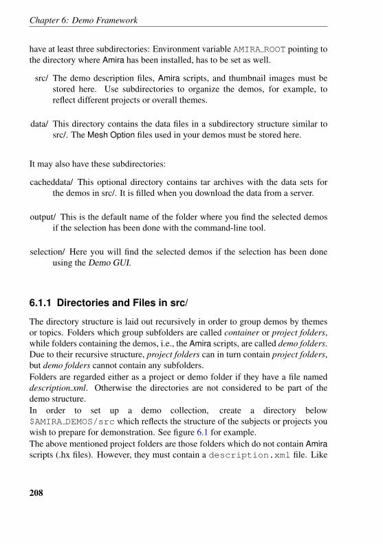
Chapter 6: Demo Framework
have at least three subdirectories: Environment variable AMIRA ROOT pointing tothe directory where Amira has been installed, has to be set as well.
src/ The demo description files, Amira scripts, and thumbnail images must bestored here. Use subdirectories to organize the demos, for example, toreflect different projects or overall themes.
data/ This directory contains the data files in a subdirectory structure similar tosrc/. The Mesh Option files used in your demos must be stored here.
It may also have these subdirectories:
cacheddata/ This optional directory contains tar archives with the data sets forthe demos in src/. It is filled when you download the data from a server.
output/ This is the default name of the folder where you find the selected demosif the selection has been done with the command-line tool.
selection/ Here you will find the selected demos if the selection has been doneusing the Demo GUI.
6.1.1 Directories and Files in src/
The directory structure is laid out recursively in order to group demos by themesor topics. Folders which group subfolders are called container or project folders,while folders containing the demos, i.e., the Amira scripts, are called demo folders.Due to their recursive structure, project folders can in turn contain project folders,but demo folders cannot contain any subfolders.Folders are regarded either as a project or demo folder if they have a file nameddescription.xml. Otherwise the directories are not considered to be part of thedemo structure.In order to set up a demo collection, create a directory below$AMIRA DEMOS/src which reflects the structure of the subjects or projects youwish to prepare for demonstration. See figure 6.1 for example.The above mentioned project folders are those folders which do not contain Amirascripts (.hx files). However, they must contain a description.xml file. Like
208
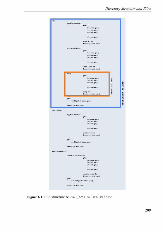
Directory Structure and Files
Figure 6.1: File structure below $AMIRA DEMOS/src
209
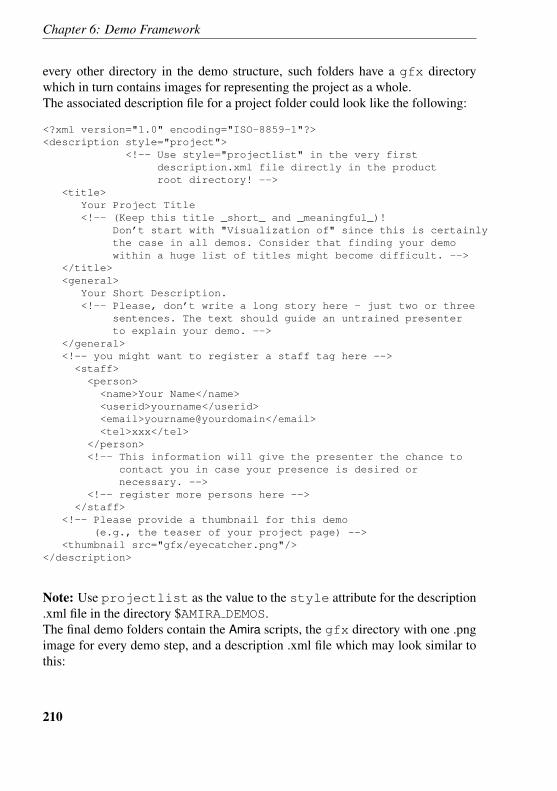
Chapter 6: Demo Framework
every other directory in the demo structure, such folders have a gfx directorywhich in turn contains images for representing the project as a whole.The associated description file for a project folder could look like the following:
<?xml version="1.0" encoding="ISO-8859-1"?><description style="project">
<!-- Use style="projectlist" in the very firstdescription.xml file directly in the productroot directory! -->
<title>Your Project Title<!-- (Keep this title _short_ and _meaningful_)!
Don’t start with "Visualization of" since this is certainlythe case in all demos. Consider that finding your demowithin a huge list of titles might become difficult. -->
</title><general>
Your Short Description.<!-- Please, don’t write a long story here - just two or three
sentences. The text should guide an untrained presenterto explain your demo. -->
</general><!-- you might want to register a staff tag here --><staff>
<person><name>Your Name</name><userid>yourname</userid><email>yourname@yourdomain</email><tel>xxx</tel>
</person><!-- This information will give the presenter the chance to
contact you in case your presence is desired ornecessary. -->
<!-- register more persons here --></staff>
<!-- Please provide a thumbnail for this demo(e.g., the teaser of your project page) -->
<thumbnail src="gfx/eyecatcher.png"/></description>
Note: Use projectlist as the value to the style attribute for the description.xml file in the directory $AMIRA DEMOS.The final demo folders contain the Amira scripts, the gfx directory with one .pngimage for every demo step, and a description .xml file which may look similar tothis:
210
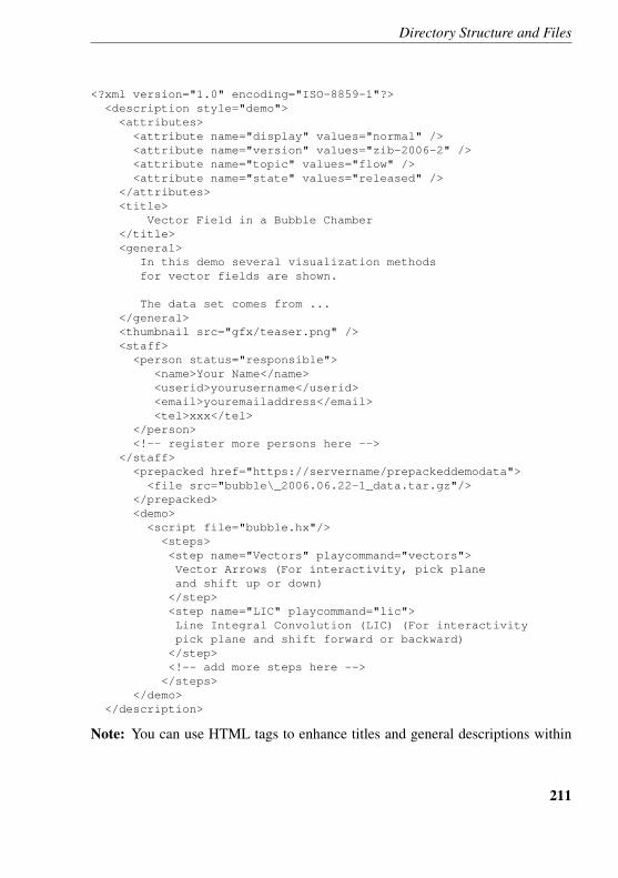
Directory Structure and Files
<?xml version="1.0" encoding="ISO-8859-1"?><description style="demo">
<attributes><attribute name="display" values="normal" /><attribute name="version" values="zib-2006-2" /><attribute name="topic" values="flow" /><attribute name="state" values="released" />
</attributes><title>
Vector Field in a Bubble Chamber</title><general>
In this demo several visualization methodsfor vector fields are shown.
The data set comes from ...</general><thumbnail src="gfx/teaser.png" /><staff>
<person status="responsible"><name>Your Name</name><userid>yourusername</userid><email>youremailaddress</email><tel>xxx</tel>
</person><!-- register more persons here -->
</staff><prepacked href="https://servername/prepackeddemodata">
<file src="bubble\_2006.06.22-1_data.tar.gz"/></prepacked><demo>
<script file="bubble.hx"/><steps><step name="Vectors" playcommand="vectors">Vector Arrows (For interactivity, pick planeand shift up or down)</step><step name="LIC" playcommand="lic">Line Integral Convolution (LIC) (For interactivitypick plane and shift forward or backward)</step><!-- add more steps here --></steps>
</demo></description>
Note: You can use HTML tags to enhance titles and general descriptions within
211
Chapter 6: Demo Framework
the description file. The XSL parser is very strict, so always use a /> at the end forsingle tags like br or p. Also be aware of the quite cumbersome encoding details.If you are writing German with umlauts, be sure that your editor also stores thesecharacters as ISO-8859-1 encoding, also known as Latin1. Otherwise you will getsurprising results in your HTML output.Each description file has a <title> and a <general> tag. Inside a <demo>tag there must be a <script> tag and a <steps> tag filled with <step> tags.The <demo> tag can have an additional attribute, stepmode, which can be setto random or static. The latter should only be used for demos, where thesequence of demo steps is strictly required (e.g., later steps rely on data loaded byearlier steps etc.). If no stepmode is specified, random is assumed.The <script> tag has a filename of an Amira-script as an attribute. This scriptis executed whenever the corresponding demo is started. Use it to define Tcl pro-cedures for subsequent steps and to load necessary data sets and modules.The <step> tag takes an optional name and a mandatory playcommand at-tribute. An option is to register a jumpcommand attribute. Please write a shortbut meaningful description for each step. That way untrained users have a chanceof presenting your demo as well.The content of playcommand is executed as a Tcl command to display the cor-responding step. The content of jumpcommand is executed as a Tcl command tojump to the beginning of a step and display the first image. This is useful if onewants to explain something before the step is executed.In demo description files only, the <description> tag may contain an optional<prepacked> tag that specifies the files to download. .tar files are untarredautomatically by downloadData.tcl, and .tar.gz files are gunzipped be-fore. You can register any number of <file> tags inside <prepacked>. Thedata to be tarred in order to use it as a prepacked file should be stored relative to$AMIRA DEMOS in a directory called $AMIRA DEMOS/data.Also only in demo description files a <attributes> tag could be used to allowa demo categorization by the search algorithm of the Demo GUI.A <staff> tag filled with <person> tags of which one may have the parameterstatus=”responsible” can be registered below <description> also.If you compiled your demo using DemoMaker, you are in good shape. Typing<DemoMakerName> writeDescriptionFile in the Amira console win-dow pops up a file browser. An appropriate description.xml file is writtenwith jumpcommand and playcommand supplied correctly. All you have to dois fill in the descriptions for the demo as a whole and for each step. Also, replacethe step names with more descriptive ones.
212
Directory Structure and Files
Also a title must be given before the description.xml file will work.A description file that does not follow the conventions mentioned above will beskipped when parsing of the demo file tree takes place.
Creating thumbnail pictures
Besides the explanation of the demo in the description file, a thumbnail image canbe helpful to show what kind of view one can expect from a particular presentation.Thumbnails are shown in the Demo GUI and in the Amira help window when it isused for demo steering. Furthermore demos can be started and steered with a webbrowser. See below.If you have prepared your demos and set up selec-tion as described below, start Amira and type: source
$AMIRA DEMOS/<outputfolder>/<demodirectory>/makeSnapshots.hx
in the Amira console. Here <outputfolder> is ’selection’ by defaultor, when using the command line tools, ’output’ resp. the name specifiedin the -o option of prepareDemos.tcl. After that there are as manystep<N>.png files as there are steps defined in the description file in a directory$AMIRA DEMOS/src/<demodirectory>/gfx/.If for some reason you need manually created thumbnails for a par-ticular demo, proceed as follows: Start that demo, and invoke source$AMIRA DEMOS/setup/makeIcon.hx. After that a Tcl proceduremakeIcon has been defined. Call it in the Amira console with makeIcon"<thumbnail filename>" <width> <height>. Do not give a file-name extension, .png will be added automatically by makeIcon. If both valuesfor width and height are given, the viewer will be resized accordingly. If one ofthese values set to 0, the viewer image will be scaled using Lanczos interpolation.Note: For better image quality, set your viewer size to a multiple of the thumbnailsize (in the default case 150x150 for thumbnails => 900x900 viewer size). Alsoconsider the contents of the viewer –if there are many small features, they won’tbe visible in the thumbnail. As is often true, less is more.Final remark: Consider the description together with the thumbnail images as astoryboard. It should describe the story you want to tell the audience while pre-senting the demonstration. Indeed you find a file storyboard.html in youroutput folder after you have setup a selection. It contains all descriptions andthumbnails of the whole selection together in one file. Useful for browsing andprinting with your favourite webbrowser.
213
Chapter 6: Demo Framework
6.1.2 Data Storage
All data being used in the demos should be stored in the $AMIRA DEMOS/data/directory. You should create a directory similar in structure to$AMIRA DEMOS/src/ for storing your data.The advantages of storing the data this way are:
• the data is separated from the script files.• a data file can easily be identified with the demo to which it belongs.• the data can be copied for pack-and-go automatically (see below).• the data can be used by several demos without needing to be duplicated.
Using a File Server to Store the Demo Data
If you want to use the same demo data sets on several computers (perhaps at differ-ent locations), it may be helpful to store the data files in a tar archive on a remotehttp server.It is beyond the scope of this documentation to explain how to set up such a server.If you decided to use a data server, define a naming scheme for your data sets andsave the data sets on the server according to that scheme. Now use the URL forthe data in your description.xml files. Be sure to create the tar files relativeto $AMIRA DEMOS.Example:The following lines of description.xml contain the data to be downloaded:
<prepacked href="https://servername/prepackeddemodata"><file src="bubble_2006.06.22-1_data.tar.gz"/>
</prepacked>
and bubble 2006.06.22-1 data.tar.gz contains:
tar tvf bubble_2006.06.22-1_data.tar... 2006-06-22 12:10:10 data/cfd/bubblechamber/... 2006-06-22 12:29:20 data/cfd/bubblechamber/physics.am... 2006-06-22 12:29:01 data/cfd/bubblechamber/Blasensaeule.surf... 2006-06-22 12:10:10 data/cfd/bubblechamber/streamsurface.surf... 2006-06-22 12:29:20 data/cfd/bubblechamber/Vektorfeld_GW_01.am
In order to fetch all data sets, you must download them as follows prior to startingthe demos:
214
Selecting Demos
cd $AMIRA_DEMOS/hxdemos/srctclsh $AMIRA_DEMOS/hxroot/share/hxdemos-scripts/downloadData.tcl
downloadData.tcl has no parameters or options!Note: downloadData.tcl downloads ALL data files mentioned in theprepacked tag of the description.xml files found in the recursively tra-versed directory tree! All downloaded files are stored in the directory$AMIRA DEMOS/cacheddata. Before downloadData.tcl downloads thefiles from the server, it checks to see if the files scheduled for downloading arealready in the cacheddata directory. This ensures that a possibly time-consumingdownload is done only once. Then all files with the extensions .tar, .tar.gzor .tgz are unpacked to $AMIRA DEMOS/data while all other files are copiedto that folder. Depending on the amount of data you stored on your data server,this may take a quite a while and use a lot of disk space.See below for downloading only those data files which are needed for a certaindemo selection.
6.2 Selecting Demos
Demos can be selected in two ways:
1. The most preferable way is to use the Demo GUI, or2. to use the command-line tool prepareDemos.tcl.
Demo GUI
The Demo GUI provides a very convenient way for selecting demos from a poolof available demos. It is also possible to change a demo selection afterwards. Ademo selection can be saved in an Amira script file for running it later. For moreinformation, see the Demo GUI documentation.
Command-line Tools
If for any reason the Demo GUI couldn’t be used to select demos, you can use acommand-line tool prepareDemos.tcl to do the selection.The command-line tools are stored under$AMIRA ROOT/share/hxdemos-scripts.
215
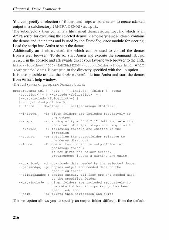
Chapter 6: Demo Framework
You can specify a selection of folders and steps as parameters to create adaptedoutput in a subdirectory $AMIRA DEMOS/output.The subdirectory then contains a file named demosequence.hx which is anAmira script for executing the selected demos. demosequence.demo containsthe demos and their steps and is used by the DemoSequence module for steering.Load the script into Amira to start the demos.Additionally an index.html file which can be used to control the demosfrom a web browser. To do so, start Amira and execute the command httpdstart in the console and afterwards direct your favorite web browser to the URLhttp://localhost:7000/<$AMIRA DEMOS>/<outputfolder>/index.html where<outputfolder> is output or the directory specified with the -o option.It is also possible to load the index.html file into Amira and start the demosfrom Amira’s help window.The full syntax of prepareDemos.tcl is
prepareDemos.tcl [--help | {[--include] {folder [--steps<steplist>]}* | --exclude <folderlist> }* |[--datainclude <folderlist>*] |[--output <outputfolder>] |[--force | --download | --[all]packandgo <folder>]
--include, -i: given folders are included recursively tothe output
--steps, -s: string of type "5 8 2 1" defining selectionand order of steps, steps starting from 1
--exclude, -e: following folders are omitted in therecursion
--output, -o: specifies the outputfolder relative tothe demos directory
--force, -f: overwrites content in outputfolder orpackandgo-folder;if not given and folder exists,prepareDemos issues a warning and exits
--download, -d: downloads data needed by the selected demos--packandgo, -p: copies output and needed data to the
specified folder--allpackandgo : copies output, all from src and needed data
to the specified folder--datainclude : given folders are included recursively to
the data folder, if --packandgo has beenspecified, too
--help, -h: prints this helpscreen and exits
The -o option allows you to specify an output folder different from the default
216
Selecting Demos
folder named output. If the packandgo option is given at the same time thisfolder will be created under the pack-and-go folder.The --packandgo option copies all files recursively from the$AMIRA DEMOS/src folder to a directory src under the folder specifiedfor this option. The needed data sets are then copied from the directory$AMIRA DEMOS/cacheddata into that folder, too. After that, you mustunpack these tar files relative to the pack-and-go folder.In order to have the data ready in cacheddata, specify the --download option.As an alternative way to provide the needed data it is possible to supply a--datainclude option in conjunction with the --packandgo option. Thisoption must have a selection of pathnames relative to $AMIRA DEMOS/datawhich are copied to a data folder under the pack-and-go folder.It is now possible to set the $AMIRA DEMOS environment variable to the pack andgo folder.Note: Be sure not to have any ”/” (slash) at the end of a path since this leads towrong results. Please, don’t use the options --datainclude and --includetogether in conjunction with --packandgo, cause it copies way too much intothe packandgo folder.Example:cd $AMIRA DEMOS/src
tclsh $AMIRA ROOT/share/hxdemos-scripts/prepareDemos.tcl
cfd/bubblechamber medicine/hyperthermia -s "1 2 5"
--download --output mydemo
This selects the entire bubble chamber demo and three steps from the hyperthermiademo and stores the necessary files in $AMIRA DEMOS/mydemo. The requesteddata sets for the two demos are stored under $AMIRA DEMOS/data if there is a<prepacked> tag in the appropriate description files.On Unix/Linux systems start Amira with $AMIRA ROOT/bin/start$AMIRA DEMOS/mydemo/demosequence.hx and on Windows systemsload $AMIRA DEMOS/mydemo/demosequence.hx just after Amira has beenstarted.Pack-and-Go Example:tclsh $AMIRA ROOT/share/hxdemos-scripts/prepareDemos.tcl
--packandgo /media/disk/hxdemos brusselator
microvisu/gigamosaic microvisu/synchrotron
microvisu/smallnetwork
This creates a folder named hxDemos under /media/disk/, selects four de-mos and puts the output into that folder. You also find under that folder the needed
217
Chapter 6: Demo Framework
data as tar files, named as described in the appropriate description .xml file.
6.3 Prerequisites
The following system tools and programs are used by Demo Framework:
• A recent version of tclsh and xsltproc is required for the scriptsprepareDemos.tcl and downloadData.tcl.
• wget and either gtar or gzip and tar is required fordownloadData.tcl.
On Unix/Linux systems all tools should already be installed.On Windows systems all tools should already be installed in cygwin as well. Ifxsltproc is missing, it is part of the package libxslt. Make sure that thePATH environment variable includes cygwin/bin to be able to use it via execin Tcl scripts.
218

Part II
Molecular Option User’sGuide
219

7 Molecular Option Introduction
Molecular Option is an Amira extension providing support for the visualization aswell as the analysis of molecules and dynamic molecular data.The Molecular Option documentation is organized into the following sections:
• Getting started with molecular visualization• Structure and interdependence of the molecular data structures• Essentials for displaying a molecule• Alignment facilities in Molecular Option
• Visualizing dynamic data• Atom expressions
7.1 First Steps with Molecular Visualization inAmira
This chapter gives you an overview of the visualization of molecular data sets.Amira is not just able to display a 3D image of the molecule but also provides toolsto investigate its distinct parts and properties. After reading the ”getting started”introduction you may continue with any of the following tutorials.
• Getting Started - first steps• Selection, Labeling, and Masking - exploring a molecule• Alignment of Molecules - visualizing dynamical data• Molecular surfaces - wrapping a molecule• Sequential and Structural Alignment - comparing molecules• Molecule Editor - interactive manipulation of the molecule• Molecular Interface - computing intersection surfaces• Measurement - measuring distances and angles within a molecule
221
Chapter 7: Molecular Option Introduction
Note: If you want to visualize your own data, please refer to the section about dataimport in the Amira User’s Guide. That section contains some general hints onhow to import data sets into Amira.
7.1.1 Getting Started with Molecular Visualization
In this section you will learn how to
1. load a molecular demo data set into Amira,2. view the molecule with the MoleculeView display module,3. try out various color schemes,4. select atoms in the viewer using the draw tool,5. overwrite color scheme colors for selected atoms.
7.1.1.1 Loading Data into the System
In the following introduction we will consider a simple example to explain thebasic functions of the MoleculeView module. Our example will be a small PDB(Protein Data Bank) structure consisting of 932 atoms in 213 residues.
• Load the file 2RNT.pdb into the Pool from the directorydata/molecules/pdb.
A green icon labeled 2RNT.pdb will appear in the Pool. The green icon repre-sents an object of type Molecule. Click on the green data icon with the left mousebutton. In the Properties Area below the Pool information about the molecule, suchas the number of atoms etc., will be shown. In addition, other ports named Trans-formation, Selection Browser, and Transform, can be seen; they will be explainedin later tutorials.
7.1.1.2 Displaying the Molecule with the MoleculeView Module
The MoleculeView module is the basic display module for visualizing molecules.It allows you to display atoms as plates or balls and bonds as lines or cylinders.
• Click again on the green data icon in the Pool, this time using the rightmouse button.
A menu, containing several entries and submenus, will appear.
222
First Steps with Molecular Visualization in Amira
• Select the entry MoleculeView.
A new yellow icon labeled MoleculeView appears in the Pool. Yellow icons,in general, represent display modules, i.e., modules that visualize objects in theviewer. The blue line between the icons indicates a connection between the ob-jects. In this case the MoleculeView module reads data from the object representedby the green icon and visualizes it.The molecule is now displayed in the viewer as a wireframe. Using the left mousebutton you can rotate the object; using the left and middle mouse buttons simulta-neously you can zoom in and out. For these mouse operations to work, the viewermust be in viewing mode, in which case the mouse cursor is displayed as a hand.Whenever the MoleculeView module is active, the little square on the yellowMoleculeView icon is orange. You can deactivate the module by clicking onthe square with the left mouse button.We will explore some basic ports of the MoleculeView module.Mode port: Choose another mode to see both atoms and bonds of the molecule, orjust atoms. If atoms are shown, use the Atom Radius port to adjust the size of theatoms as desired.Quality port: If you choose the option correct, you can display a correct, i.e. three-dimensional, image of the balls and sticks. Consider the trade-off between correctrepresentation and slower rendering performance. Use the fast mode if you wantto display a large molecule. If your graphics hardware is fast enough, you can usethe correct mode even for large molecules.Complexity port: In order to allow interactive rendering, the default complexity ofthe scene is rather low. In most cases this will be sufficient. However, if you wantto make screen shots or if you have small molecules, you might want to increasethe complexity. The Complexity port is displayed only if correct quality is selected.
7.1.1.3 Changing the Color Scheme
The MoleculeView module allows the user to color the molecule according tolevels, for example, atom level, residue level, secondary structure level, chain level,or user-defined levels. Each level has a number of attributes, the simplest of whichis the index attribute. The default color scheme is to color the molecule accordingto the atom level’s attribute atomic number, i.e., the atom’s type.
• Click the Legend button of the Color port to display a small window decod-ing the colors you see in the viewer window.
223
Chapter 7: Molecular Option Introduction
• Choose residues from the first pop-up menu and type from the second menuto color the molecule according to the residue type, here the amino acidtype.
The default colormap contains a constant color. Thus, currently all residues of themolecule have the same color.
• To change the colormap, right-click on the color bar of the Discrete CM portwhich has appeared below the Color port and select any other colormap.
• Try out different colormaps to find a map that suits your purposes.
Some people prefer the CPK color scheme for atoms and the amino acid colors asthey are used in the RasMol program.
• You can set your preferences in the AmiraEdit menu by selecting the entryPreferences.
• Press the Molecules tab and set your preferences. Pressing the OK buttonsaves your preferences permanently.
Currently only amino acid colors are predefined. Thus, if the molecule containsresidues other than the standard amino acids, those residues will be colored withthe default color (black).
7.1.1.4 Using the Draw Tool
The draw tool appears in Amira in several modules. It enables you to select objectsor parts of an object by drawing a line in the viewer.
• Press the Draw button of the Highlighting port and draw a line in the viewerwindow around the group of atoms you want to select.
The atoms that were enclosed by the line will be highlighted. If the viewer is theactive window, pressing the d key is equivalent to pressing the Draw button of theHighlighting port.
• To unhighlight all atoms, press the Clear button of the Highlighting port.• Also try using the keys Ctrl and Shift while drawing a line.
7.1.1.5 Setting Colors for Selected Parts
The Define Colors port allows you to overwrite colors of the color scheme.
224
First Steps with Molecular Visualization in Amira
• Select some atoms using the draw tool.• Press the Set button of the Define Color port.• Change the current color of the Color Editor and press OK.
The previously highlighted atoms should now have the color selected in the coloreditor. This setting will be preserved even if the color scheme is changed. Unfor-tunately, the new setting will currently not appear in the color legend.
7.1.2 Selection, Labeling, and Masking
You already know how to load files and how to display molecules with theMoleculeView module. This tutorial will focus on exploring the structure of aloaded molecule. The tutorial consists of three subsections, in which you will:
1. Explore the possibilities for selecting within a molecule using the Molecule-View module.
2. Learn how to use the MoleculeLabel module.3. Get to know the Molecule Selection Browser.
For this tutorial we will use the molecule 1IGM.pdb.
• Load the file 1IGM.pdb into the Pool from the directorydata/molecules/pdb.
• Attach a MoleculeView module to the green object that has appeared,• and change the Mode port to balls and sticks.
7.1.2.1 Interactive Selection with the MoleculeView Module
In the first tutorial you learned how to use the draw tool to select atoms within amolecule. The simplest way to select atoms, however, is to click on the atom ofinterest. In order to do so, the viewer must be in interaction mode. If the mousecursor in the viewing window is depicted as a hand, you are in viewing mode. Tochange to interaction mode, you can either
• click on the arrow button in the upper right corner of the viewing windowor press the Esc button while the viewing window is active.
The mouse cursor will change to an arrow.
• Now click one of the atoms.
225
Chapter 7: Molecular Option Introduction
The atom you selected should now be highlighted by a red frame around it. If youselect another atom, the first atom will be unhighlighted. In order to select morethan one atom
• press the Ctrl key and keep it pressed while clicking additional atoms.
Ctrl-clicking a highlighted atom a second time unhighlights it.
• Now change the Mode port of the MoleculeView back to sticks.• Select residues from the first menu of the MoleculeView’s Color port.• Choose a suitable colormap from the list of pre-loaded colormaps as de-
scribed in the first tutorial.
The residues should now be colored according to their type.
• Now select an atom.
As result the whole residue should now be highlighted. The reason for this isthat picking is bound to the coloring, by default. For example, if the colorscheme is atoms, a click on an atom will only influence the selection for thisatom; if the scheme is residues, the atom’s residue will be selected; if it ischains, the atom’s chain will be selected, and so on. However, since this isvery restrictive you can easily change the selection mode to the most com-mon levels, i.e., atoms, residues, secondary structures, and chains. In order tochoose a certain level for the selection you need to press certain keys in advance.Ctrl-Alt-Shift-a chooses the atoms level, a click on an atom will only influ-ence the selection for this atom. Ctrl-Alt-Shift-r, Ctrl-Alt-Shift-cand Ctrl-Alt-Shift-s choose residues, chains and secondary structure levelrespectively. To switch back to the default behavior, where coloring determines se-lection, press Ctrl-Alt-Shift-d.If you select some group and afterwards select a second one from the same levelholding down the Shift-key all groups between the two will also be selected.Holding the Ctrl-key pressed while selecting groups allows you to select multiplegroups and also to toggle a group when selecting it a second time.If you do any selection by clicking in the viewer there will be some output inthe console window informing you about what you have selected, the amount ofoutput can be customized via the Preferences dialog:
• You can set your preferences in the AmiraEdit menu by selecting the entryPreferences.
226
First Steps with Molecular Visualization in Amira
• Press the Molecules tab and take a look on the options in chapter SelectionInfo:
• Molecule name determines that the name of the molecule, to which a se-lected group belongs, will be printed.
• Group name determines that the name of the selected group will be printed.• Group attributes determines that not only the selected group’s name but
also all attribute values of the group will be printed in the console window.• Explicit attributes restricts the output of attribute values to those attributes
that are explicitly named in the text field.• Pressing the OK button saves your preferences permanently.
7.1.2.2 Using the MoleculeLabel Module
So far you have seen that you can select atoms and groups of atoms by clicking onthe molecule. The result of the picking is always printed in the console window.This might suffice in some cases. In other cases, however, it is necessary to labelthe molecule in the viewer so that you can easily track certain groups you areinterested in. If you want to use this tool, here is how you do it.
• Click again on the icon 1IGM.pdb with the right mouse button.• Select MoleculeLabel from the Display submenu.
A second yellow icon labeled MoleculeLabel should have appeared in the Pool.By default, all clicks will now be handled by the MoleculeLabel module. Thismeans that instead of highlighting groups when clicking on them they will nowget labeled.
• Type Ctrl-Alt-Shift-r while the viewing window is active.• Click on the molecule in the 3D viewer.
This action should cause the residue of the selected atom to get labeled. Press-ing Ctrl-Alt-Shift-a and clicking the same atom will result in the selectedatom being labeled. The Ctrl- and Shift- keys have the same effect as whenselecting groups.
• Label a few residues and atoms.• Click on the MoleculeLabel icon to view its ports in the Properties Area.• Change the color of the atom labels by pressing the color button of the Color
port and selecting a different color in the color editor.
227
Chapter 7: Molecular Option Introduction
• Now select residues in the Levels port. The Attributes, Level Option, But-tons, Font Size, and Color ports now affect the residue labels.
• Increase the font size (which only increases the font size of the current level,i.e., residues).
• Select the name entry in the second menu of the Attributes port.
The selected residues will now be labeled by their types and names. In order tounderstand the Options port of the MoleculeLabel module
• deselect the last option, replace attributes,• and set the entry of the second Attributes menu back to disabled.• Now select a new residue, holding the Ctrl- key down.
The new residue will only be labeled by its type. In contrast, the old residues arestill labeled with type and name.If the first option of the last port, handle clicks, is deselected, mouse clicks will behandled just as if the module MoleculeLabel did not exist.
• Deselect the handle clicks option.• Select any residue.
The residue is selected, not labeled.
7.1.2.3 Molecule Selection Browser
In this section you will learn the basics about the molecule selection browser,which is a very important feature for the investigation of a molecule. The selectionbrowser is a flexible tool for selecting those parts of the molecule that you areinterested in. Moreover, it allows you to easily combine different viewing modulesinto one viewer.
• Select the green icon 1IGM.pdb by clicking on it.• Press the Show button of the Selection Browser port to open the browser.
The scroll view of the browser currently contains three columns, one with theheading level/name, the second with the heading type, and the third with the head-ing MV which stands for MoleculeView. In the first column, all residues of themolecule are displayed. The second column shows the residue type.
• Connect a BondAngleView to 1IGM.pdb by right-clicking the icon andchoosing BondAngleView from the Display submenu.
228
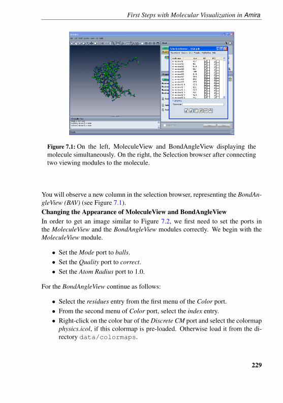
First Steps with Molecular Visualization in Amira
Figure 7.1: On the left, MoleculeView and BondAngleView displaying themolecule simultaneously. On the right, the Selection browser after connectingtwo viewing modules to the molecule.
You will observe a new column in the selection browser, representing the BondAn-gleView (BAV) (see Figure 7.1).Changing the Appearance of MoleculeView and BondAngleViewIn order to get an image similar to Figure 7.2, we first need to set the ports inthe MoleculeView and the BondAngleView modules correctly. We begin with theMoleculeView module.
• Set the Mode port to balls.• Set the Quality port to correct.• Set the Atom Radius port to 1.0.
For the BondAngleView continue as follows:
• Select the residues entry from the first menu of the Color port.• From the second menu of Color port, select the index entry.• Right-click on the color bar of the Discrete CM port and select the colormap
physics.icol, if this colormap is pre-loaded. Otherwise load it from the di-rectory data/colormaps.
229
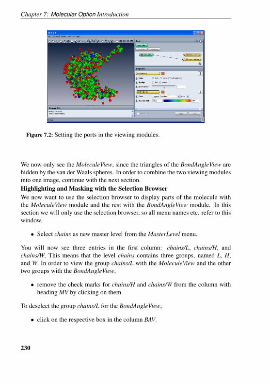
Chapter 7: Molecular Option Introduction
Figure 7.2: Setting the ports in the viewing modules.
We now only see the MoleculeView, since the triangles of the BondAngleView arehidden by the van der Waals spheres. In order to combine the two viewing modulesinto one image, continue with the next section.Highlighting and Masking with the Selection BrowserWe now want to use the selection browser to display parts of the molecule withthe MoleculeView module and the rest with the BondAngleView module. In thissection we will only use the selection browser, so all menu names etc. refer to thiswindow.
• Select chains as new master level from the MasterLevel menu.
You will now see three entries in the first column: chains/L, chains/H, andchains/W. This means that the level chains contains three groups, named L, H,and W. In order to view the group chains/L with the MoleculeView and the othertwo groups with the BondAngleView,
• remove the check marks for chains/H and chains/W from the column withheading MV by clicking on them.
To deselect the group chains/L for the BondAngleView,
• click on the respective box in the column BAV.
230
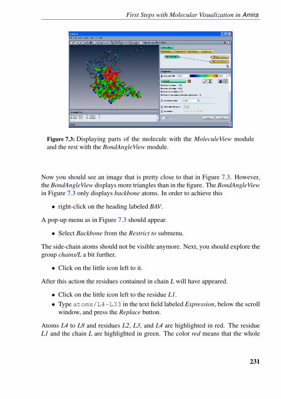
First Steps with Molecular Visualization in Amira
Figure 7.3: Displaying parts of the molecule with the MoleculeView moduleand the rest with the BondAngleView module.
Now you should see an image that is pretty close to that in Figure 7.3. However,the BondAngleView displays more triangles than in the figure. The BondAngleViewin Figure 7.3 only displays backbone atoms. In order to achieve this
• right-click on the heading labeled BAV.
A pop-up menu as in Figure 7.3 should appear.
• Select Backbone from the Restrict to submenu.
The side-chain atoms should not be visible anymore. Next, you should explore thegroup chains/L a bit further.
• Click on the little icon left to it.
After this action the residues contained in chain L will have appeared.
• Click on the little icon left to the residue L1.• Type atoms/L4-L33 in the text field labeled Expression, below the scroll
window, and press the Replace button.
Atoms L4 to L8 and residues L2, L3, and L4 are highlighted in red. The residueL1 and the chain L are highlighted in green. The color red means that the whole
231
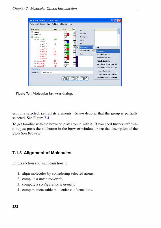
Chapter 7: Molecular Option Introduction
Figure 7.4: Molecular browser dialog.
group is selected, i.e., all its elements. Green denotes that the group is partiallyselected. See Figure 7.4.
To get familiar with the browser, play around with it. If you need further informa-tion, just press the F1 button in the browser window or see the description of theSelection Browser.
7.1.3 Alignment of Molecules
In this section you will learn how to
1. align molecules by considering selected atoms,2. compute a mean molecule,3. compute a configurational density,4. compare metastable molecular conformations.
232
First Steps with Molecular Visualization in Amira
7.1.3.1 Comparing two Molecules
In this section we will compare two different three-dimensional structures of thesame molecule.
• Load the data file alkane.zmf from the directorydata/molecules/alkane.
• Select MolTrajectory from the pop-up menu of the alkane.zmf icon.• Select Molecule from the pop-up menu of the MolTrajectory icon.• Attach a MoleculeView module to the molecule.• Repeat the last two steps, creating two new objects, Molecule2 and
MoleculeView2
The alkane.zmf icon represents a bundle of molecular trajectories, in this case bu-tane, pentane, and hexane. By attaching a MolTrajectory to it, we extract a singletrajectory. By default, the first trajectory, which is butane, is selected. We can nowextract single time steps from the trajectory by attaching a Molecule object to thetrajectory. We have done this twice since we want to compare two time steps witheach other. Currently, both molecules extract the same time step. This is the reasonfor only seeing a single molecule. In order to get more information about the datastructures, go to the section on molecular data structures.
• Select the MoleculeView icon and change the Mode port to balls and sticksand the Quality port to correct.
• Repeat this action for the MoleculeView2.• Select the Molecule2 icon and change the value of the Time port to 2.
You should now see two butane molecules in the viewer, slightly displaced.
• Right-click on the white square at the far left side of the Molecule2 icon andselect AlignMaster from the pop-up menu.
• Connect the blue line to the Molecule icon.• Select the Molecule2 icon.• Press the all button of Molecule2’s Select port.
You have now aligned the molecules Molecule and Molecule2 using a least squaresfitting of all atoms. This only works for molecules with the same number of atoms.In the following we will align the two molecules by considering only three carbonatoms.
233
Chapter 7: Molecular Option Introduction
• Deactivate the MoleculeView by clicking on the orange square of theMoleculeView icon.
• Ctrl-click on three consecutive carbon atoms.
The frame of a red cube should appear around each of them.
• Activate the MoleculeView by clicking on the gray square on the Molecule-View icon.
• Select the Molecule2 icon and press the in slave button of the Select port.
The three selected atoms should now fit better onto the corresponding atoms of theobject labeled Molecule.
7.1.3.2 Computing a Mean Molecule
In this section we will compute a mean molecule of a metastable molecular con-formation of butane.
• Remove the objects Molecule and Molecule2.• Select the MolTrajectory icon.• Load the data file but cluster 3 1.idx from the directorydata/molecules/alkane.
but cluster 3 1.idx is a subtrajectory of MolTrajectory, i.e., a subset of all config-urations in the trajectory.
• Attach a molecule to the icon but cluster 3 1.idx.• Select the MeanMolecule entry from the Compute submenu of
but cluster 3 1.idx’s pop-up menu.• Right-click with the mouse on the white square at the far left side of the
MeanMolecule icon and select AlignMaster.• Connect the AlignMaster port to the Molecule icon by attaching the blue
line to it.• Select the MeanMolecule icon and press the all button of the Select port of
the MeanMolecule module.• Press the Apply button to compute the mean molecule.• Visualize the mean molecule but cluster 3 1.mean by attaching a Molecule-
View to it.
234
First Steps with Molecular Visualization in Amira
• Connect the AlignMaster port of the module MeanMolecule to thebut cluster 3 1.mean icon.
• Press the Apply button of the MeanMolecule module two or three times.
You have now computed a mean molecule of the subtrajectory but cluster 3 1.idx.The AlignMaster is used to align all time steps before accumulating the atom posi-tions. Changing the AlignMaster to the previously computed mean molecule andrepeating the computation of the mean molecule will improve it. This procedureshould converge.
A better way to compute a mean molecule is to use the module PrecomputeAlign-ment, using the Multiple Alignment option of the Mode port. This module createsan object containing a transformation for each structure in the trajectory. This ob-ject can then get connected to the PrecomputeAlignment connection port of theMeanMolecule module.
7.1.3.3 Computing and Visualizing a Configuration Density
For the subset of configurations contained in the subtrajectory but cluster 3 1.idx,we will now compute a configuration density and visualize it with the Isosurfacedisplay module.
• Select the entry ConfigurationDensity from the Compute submenu ofbut cluster 3 1.idx’s pop-up menu.• Connect the AlignMaster port of the ConfigurationDensity icon to the
but cluster 3 1.mean icon.• Select the ConfigurationDensity icon.• Press the all button of the Select port.• Press the Field button of the Compute port to compute the density.• Visualize the created scalar field but cluster 3 1.scalar with an isosurface
by first selecting the Isosurface entry from the Display submenu of theicon’s pop-up menu,
• second, setting the Isosurface’s Threshold value to 0.1,• and third, pressing the Apply button.• Try different Threshold values.
235
Chapter 7: Molecular Option Introduction
7.1.3.4 Comparing Metastable Molecular Conformations
The set of configurations in the subtrajectory but cluster 3 1.idx belongs to ametastable conformation of butane. In this section we will compute the densityof a second metastable conformation and compare the two with each other.
• Select the MolTrajectory icon.• Load the data file but cluster 3 2.idx from the directorydata/molecules/alkane.
• Compute the mean molecule of the subtrajectory but cluster 3 2.idx by re-peating the steps described above for the subtrajectory but cluster 3 1.idx.
• Visualize the second mean molecule with the MoleculeView module.• Select three consecutive carbon atoms in the second mean molecule as was
done in the first tutorial.• Attach the AlignMaster of the object but cluster 3 2.mean to the first mean
molecule but cluster 3 1.mean.• Select the but cluster 3 2.mean icon and press the in slave button of the
mean molecule’s Select port.
The two mean molecules should now be aligned to each other, i.e., the three se-lected carbon atoms should superimpose.
• Compute the density for the second subtrajectory using thebut cluster 3 2.mean molecule as AlignMaster.
• Visualize the computed density with an Isosurface module.• Double-click on the colormap of the Isosurface2 module and select a differ-
ent color to better distinguish the two isosurfaces from each other.
You should now clearly see how the two conformations of butane differ. For largermolecules it might be interesting to color the isosurface according to the atom’scolors. This can be done using the same ConfigurationDensity modules by select-ing the Color Field option of the Field port. Attach the computed color field to theColorField connection port of the Isosurface module.
Notice that you can also visualize the densities with the Voltex module of theDisplay submenu.
236
First Steps with Molecular Visualization in Amira
7.1.4 Molecular Surfaces
In section 7.1.1 of this tutorial you have seen how to visualize molecules with theMoleculeView module. Section 7.1.2 , on selection, labeling and masking, showedyou how to use Amira’s facilities to select, mask, and label certain parts of themolecule. In this tutorial we will
1. compute a molecular surface with the CompMolSurface module,2. compute the molecular surface for a restricted set of atoms,3. compute partial surfaces,4. explore the MolSurfaceView module,5. get to know the picking facilities of the MolSurfaceView.
7.1.4.1 Compute Molecular Surfaces
In this section you will learn how to use the CompMolSurface module to computemolecular surfaces with different resolutions. You will also become familiar withsome of the module’s basic ports.
• Load the data file 2RNT.pdb from the directorydata/molecules/pdb.
• Attach the CompMolSurface module to the green icon by selecting the corre-sponding entry from the Compute submenu of 2RNT.pdb’s pop-up menu.
• Select the CompMolSurface icon.• Press the Apply button.• Attach the MolSurfaceView module to the newly created green icon,2RNT-surf.
You should now see a gray solvent excluded surface which is still pretty coarse. Ifyou want a surface with better resolution,
• increase the number of points per A2 in the CompMolSurface module.• Press the Apply button again.• Try different resolutions.• Now select the no duplicate points option in the Options port.• Press the Apply button.
Due to the last action, some sharp edges will have disappeared. If there are noduplicate points at sharp edges, the surface normals of the adjacent triangles will
237
Chapter 7: Molecular Option Introduction
be interpolated, thus leading to a smoothing, which in this case might be undesired.However, this option is important if it is necessary to have a completely closedsurface.
• Change the Quality port to faster.• Press the Apply button.
You should observe that some atoms disappear. This is due to the fact that nowonly one surface component will be computed. If the molecular surface consistsof only one component, the whole surface will be computed. Since the underlyingalgorithm does not need to touch every single atom, but approximately only everysecond atom, the algorithm is much faster. If performance is an issue, you mightconsider using this option.
7.1.4.2 Compute Partial Surfaces
In order to compute partial surfaces we need to select the atoms for which we wantto compute their surface contribution.
• Open the selection browser. If you do not know how to do this, take a lookat the second tutorial.
• Type within(residues/HET105, 5) in the browser’s Expressioncommand line.
• Press the selection browser’s Replace button.
All atoms within a distance of 5 A of the HET105 residue will now be selected.
• Reset the CompMolSurface’s Quality port back to correct.• Select partial surface from the Options port of CompMolSurface.• Press the Apply button.• Select adjacent patches from the Options port of CompMolSurface.• Press the Apply button.
The last action causes the partial surface to be expanded by the toroidal patchesadjacent to the partial surface.
7.1.4.3 Molecular Surface of a Restricted Set of Atoms
The molecule 2RNT.pdb contains some water molecules, which are in most casesnot desired when computing the molecular surface. In order to exclude the water
238
First Steps with Molecular Visualization in Amira
molecule from the surface computation
• open the selection browser again.• In the selection browser scroll to the end of the list of residues.• Click on one of the strings HOH in the type column.
All residues of type HOH should now be highlighted.
• In the browser, right-click on the heading CMS which stands for CompMol-Surface and select the entry Remove.
• Deselect partial surface in the CompMolSurface module.• Press the Apply button.
For the new surface only those residues that have a check mark in the selectionbrowser were considered. You may combine this procedure with the partial surfacecomputation described above.
7.1.4.4 Exploring the MolSurfaceView
The MolSurfaceView module is already attached to the molecular surface. A sec-ond connection exists to the molecule 2RNT.pdb, from which data is read toenhance the visualization.
• Compute the whole molecular surface with a resolution of 2 points per A2.• Click on the MolSurfaceView icon to see its user interface in the Prop-
erties Area.• Select molecule for the Color Mode.• Change the Color port’s first menu entry to residues.• Select an appropriate colormap for the Discrete CM port by right-clicking
on the color bar.• Switch to interaction mode by clicking on the arrow button in the upper right
corner of the viewing window.• Click on the surface in the viewing window.
All triangles belonging to the picked triangle’s residue will be highlighted. If thetriangle belongs to two or even three (maximum) residues, all of those residueswill be highlighted.Clicking on the surface with the middle mouse button displays information aboutthe atom you clicked on in the upper left corner of the viewing window as long
239
Chapter 7: Molecular Option Introduction
as you keep the mouse button pressed. If you Ctrl-click, the information willremain displayed even after releasing the mouse button until the next mouse clickon the surface.
• Press the Highlighting port’s Clear button to remove the selection.• Change the Pick Action port to clipping.• Pick any triangle of the surface.
All triangles further away from the picked triangle than the distance given by theSelection Distance port will be cut off. All triangles within this distance will re-main, however, only if they are connected to the picked triangle without leavingthe sphere around the picked point.
• Press the All button of the Buffer port to display the whole surface.• Change the Pick Action port to surface.• Shift-click on the surface in the viewing window.
All clicks on the surface will now be handled as you might be familiar with fromthe SurfaceView module.
7.1.5 Sequential and Structural Alignment
In this tutorial you will become familiar with the AlignSequences and Align-Molecules modules.The AlignSequences tool facilitates the comparison of two sequences. It can beapplied to both proteins and nucleic acids except for t-rna molecules containingmodified bases. The AlignSequences module is not highly advanced, but it mightsuffice for some purposes.Having done the sequential alignment, you can use the correspondence producedby the sequence alignment to do a structural alignment of the molecules.
• Load the files 1IGM.pdb and 2JEL.pdb from the directorydata/molecules/pdb/ and connect a MoleculeView to each ofthem.
You should know how to do this from the first tutorial. For both MoleculeViews
• select residues from the first menu of the Color port.
A colormap (Discrete CM) with constant color will appear. To distinguish themolecules, choose a different color for one of them. In order to do so
240
First Steps with Molecular Visualization in Amira
• double-click on the colorbar (the Color Dialog should appear) and• change the current color by dragging and dropping any of the custom colors.• Press the OK button of the color editor.
7.1.5.1 Sequence Alignment
We will now use the AlignSequences module to align the sequences of the twomolecules. In the next section we will use the associated amino acid pairs for astructural alignment.
• Right-click on the 1IGM.pdb icon and select AlignSequences from the Com-pute submenu.
• Right-click the white square on the far left side of the AlignSequences icon.
A pop-up menu displaying all connection ports opens.
• Select MoleculeB from it and connect the port to the 2JEL.pdb icon by click-ing on it.
There should now be two blue lines connecting the AlignSequences icon with the1IGM.pdb and 2JEL.pdb icons, respectively.
• Select the module AlignSequences by clicking on its icon in the Pool.• Choose semiglobal from the second menu of the Align Type port.• Press the Apply button.
If the alignment has been successful, a window displaying several slightly differentalignments will appear.
• Press the AcceptAll button. Then press the Close button.
This action results in the alignments being written to the molecules as new levels.In order to check this,
• type 1IGM.pdb list in the Amira console window.
In addition to levels such as atoms, bonds, residues, etc. you will also see levelsnamed semiGlobalSeqAlign1 to semiGlobalSeqAlign10. 2JEL.pdb has the samelevels with an equal number of groups.
241
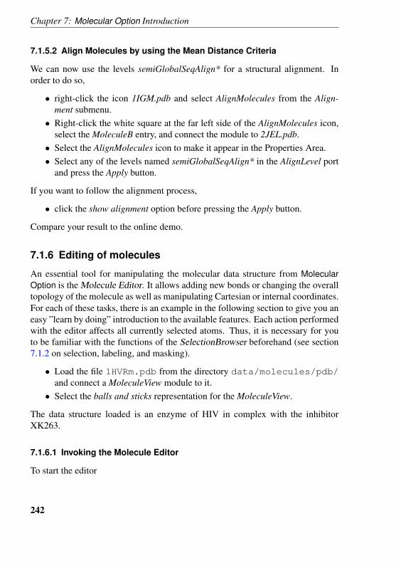
Chapter 7: Molecular Option Introduction
7.1.5.2 Align Molecules by using the Mean Distance Criteria
We can now use the levels semiGlobalSeqAlign* for a structural alignment. Inorder to do so,
• right-click the icon 1IGM.pdb and select AlignMolecules from the Align-ment submenu.
• Right-click the white square at the far left side of the AlignMolecules icon,select the MoleculeB entry, and connect the module to 2JEL.pdb.
• Select the AlignMolecules icon to make it appear in the Properties Area.• Select any of the levels named semiGlobalSeqAlign* in the AlignLevel port
and press the Apply button.
If you want to follow the alignment process,
• click the show alignment option before pressing the Apply button.
Compare your result to the online demo.
7.1.6 Editing of molecules
An essential tool for manipulating the molecular data structure from MolecularOption is the Molecule Editor. It allows adding new bonds or changing the overalltopology of the molecule as well as manipulating Cartesian or internal coordinates.For each of these tasks, there is an example in the following section to give you aneasy ”learn by doing” introduction to the available features. Each action performedwith the editor affects all currently selected atoms. Thus, it is necessary for youto be familiar with the functions of the SelectionBrowser beforehand (see section7.1.2 on selection, labeling, and masking).
• Load the file 1HVRm.pdb from the directory data/molecules/pdb/and connect a MoleculeView module to it.
• Select the balls and sticks representation for the MoleculeView.
The data structure loaded is an enzyme of HIV in complex with the inhibitorXK263.
7.1.6.1 Invoking the Molecule Editor
To start the editor
242
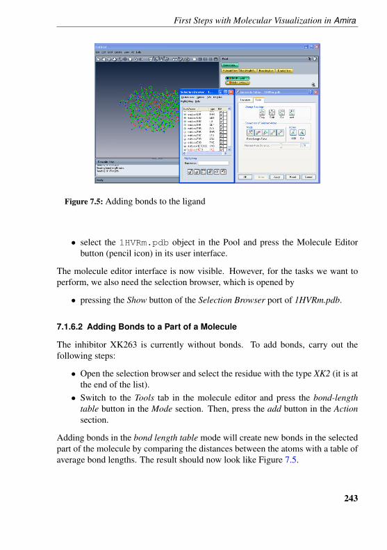
First Steps with Molecular Visualization in Amira
Figure 7.5: Adding bonds to the ligand
• select the 1HVRm.pdb object in the Pool and press the Molecule Editorbutton (pencil icon) in its user interface.
The molecule editor interface is now visible. However, for the tasks we want toperform, we also need the selection browser, which is opened by
• pressing the Show button of the Selection Browser port of 1HVRm.pdb.
7.1.6.2 Adding Bonds to a Part of a Molecule
The inhibitor XK263 is currently without bonds. To add bonds, carry out thefollowing steps:
• Open the selection browser and select the residue with the type XK2 (it is atthe end of the list).
• Switch to the Tools tab in the molecule editor and press the bond-lengthtable button in the Mode section. Then, press the add button in the Actionsection.
Adding bonds in the bond length table mode will create new bonds in the selectedpart of the molecule by comparing the distances between the atoms with a table ofaverage bond lengths. The result should now look like Figure 7.5.
243
Chapter 7: Molecular Option Introduction
7.1.6.3 Splitting the Molecule
We now want to split the molecule into inhibitor and protein.
• If it is not currently selected, reselect the XK2 residue in the selectionbrowser.
• Press the Split button on the Tools tab of the molecule editor.
You will notice that the atoms of the inhibitor are no longer displayed by theMoleculeView and that a new object, 1HVRm2.pdb, has appeared in the Pool. Thisobject contains the previously selected atoms of the ligand.
7.1.6.4 Adding another molecule
The protein of the 1HVR entry is a protease which uses up one water molecule tosplit a polypeptide. We now want to add the water to the active site of the enzyme.
• Load the file h2o.pdb from the directory data/molecules/pdb.• Go to the molecule editor and press the Add button in the Change Topology
section.• In the window that opens, all other molecules in the Pool will be shown.
Select the h2o.pdb molecule and press OK.
The atoms of the water molecule have now been copied to the 1HVRm.pdb object.
7.1.6.5 Moving Parts of the Molecule
To concentrate our view on the region of interest we will reduce the molecularview to amino acids A25 and B25 between which the water molecule should beplaced.
• Type r/name=?25 OR r/type=H2O into the selection browser andpress the Add button.
• Now move your mouse on the MV heading, press the right mouse button,and activate the Replace option.
With only the residues A25 and B25 and the water molecule displayed, all that isleft to do is to drag the water molecule to its correct location.
• Select the water molecule in the selection browser (the residue at the end ofthe list).
244
First Steps with Molecular Visualization in Amira
Figure 7.6: Moving the water molecule to the desired location
• Switch to the Transform tab of the molecule editor.
• Show the position of the transform dragger by pressing the button in thePosition section of the Transform tab.
• Left-click on the dragger and hold the mouse button down. You can nowtranslate the dragger in different planes depending on the side you clickedon. Move the water molecule between the two amino acids as shown inFigure 7.6.
• To reorient the water molecule, click on the green knobs of the dragger.They allow the dragger to rotate in different planes.
Repeat the steps described above until you are satisfied with the result.To apply the changes that you made to the edited molecule, you must press theApply button or end the editing by using the OK button.
7.1.7 Molecular Interfaces
This tool is particularly interesting for visualizing contact areas between parts ofa single molecule or between different molecules, e.g., enzymes and their ligands.In this example we will consider the second case.
245
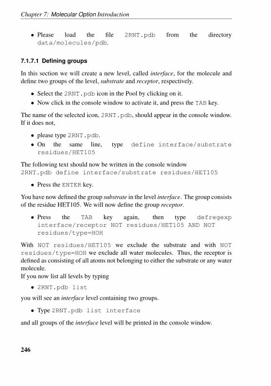
Chapter 7: Molecular Option Introduction
• Please load the file 2RNT.pdb from the directorydata/molecules/pdb.
7.1.7.1 Defining groups
In this section we will create a new level, called interface, for the molecule anddefine two groups of the level, substrate and receptor, respectively.
• Select the 2RNT.pdb icon in the Pool by clicking on it.• Now click in the console window to activate it, and press the TAB key.
The name of the selected icon, 2RNT.pdb, should appear in the console window.If it does not,
• please type 2RNT.pdb.• On the same line, type define interface/substrateresidues/HET105
The following text should now be written in the console window2RNT.pdb define interface/substrate residues/HET105
• Press the ENTER key.
You have now defined the group substrate in the level interface. The group consistsof the residue HET105. We will now define the group receptor.
• Press the TAB key again, then type defregexpinterface/receptor NOT residues/HET105 AND NOTresidues/type=HOH
With NOT residues/HET105 we exclude the substrate and with NOTresidues/type=HOH we exclude all water molecules. Thus, the receptor isdefined as consisting of all atoms not belonging to either the substrate or any watermolecule.If you now list all levels by typing
• 2RNT.pdb list
you will see an interface level containing two groups.
• Type 2RNT.pdb list interface
and all groups of the interface level will be printed in the console window.
246
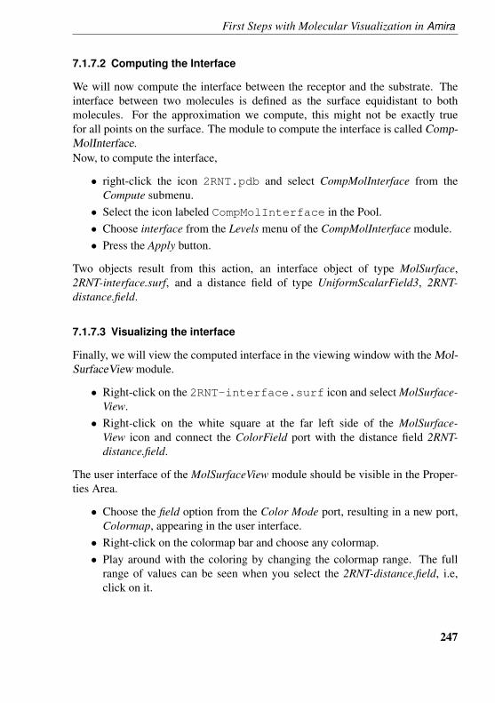
First Steps with Molecular Visualization in Amira
7.1.7.2 Computing the Interface
We will now compute the interface between the receptor and the substrate. Theinterface between two molecules is defined as the surface equidistant to bothmolecules. For the approximation we compute, this might not be exactly truefor all points on the surface. The module to compute the interface is called Comp-MolInterface.Now, to compute the interface,
• right-click the icon 2RNT.pdb and select CompMolInterface from theCompute submenu.
• Select the icon labeled CompMolInterface in the Pool.• Choose interface from the Levels menu of the CompMolInterface module.• Press the Apply button.
Two objects result from this action, an interface object of type MolSurface,2RNT-interface.surf, and a distance field of type UniformScalarField3, 2RNT-distance.field.
7.1.7.3 Visualizing the interface
Finally, we will view the computed interface in the viewing window with the Mol-SurfaceView module.
• Right-click on the 2RNT-interface.surf icon and select MolSurface-View.
• Right-click on the white square at the far left side of the MolSurface-View icon and connect the ColorField port with the distance field 2RNT-distance.field.
The user interface of the MolSurfaceView module should be visible in the Proper-ties Area.
• Choose the field option from the Color Mode port, resulting in a new port,Colormap, appearing in the user interface.
• Right-click on the colormap bar and choose any colormap.• Play around with the coloring by changing the colormap range. The full
range of values can be seen when you select the 2RNT-distance.field, i.e,click on it.
247
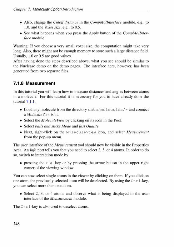
Chapter 7: Molecular Option Introduction
• Also, change the Cutoff distance in the CompMolInterface module, e.g., to1.0, and the Voxel size, e.g., to 0.5.
• See what happens when you press the Apply button of the CompMolInter-face module.
Warning: If you choose a very small voxel size, the computation might take verylong. Also, there might not be enough memory to store such a large distance field.Usually, 1.0 or 0.5 are good values.After having done the steps described above, what you see should be similar tothe Nuclease demo on the demo pages. The interface here, however, has beengenerated from two separate files.
7.1.8 Measurement
In this tutorial you will learn how to measure distances and angles between atomsin a molecule. For this tutorial it is necessary for you to have already done thetutorial 7.1.1.
• Load any molecule from the directory data/molecules/* and connecta MoleculeView to it.
• Select the MoleculeView by clicking on its icon in the Pool.• Select balls and sticks Mode and fast Quality.• Next, right-click on the MoleculeView icon, and select Measurement
from the pop-up menu.
The user interface of the Measurement tool should now be visible in the PropertiesArea. An Info port tells you that you need to select 2, 3, or 4 atoms. In order to doso, switch to interaction mode by
• pressing the ESC key or by pressing the arrow button in the upper rightcorner of the viewing window.
You can now select single atoms in the viewer by clicking on them. If you click onone atom, the previously selected atom will be deselected. By using the Ctrl-key,you can select more than one atom.
• Select 2, 3, or 4 atoms and observe what is being displayed in the userinterface of the Measurement module.
The Ctrl-key is also used to deselect atoms.
248
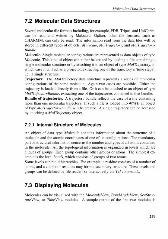
Molecular Data Structures
7.2 Molecular Data Structures
Several molecular file formats including, for example, PDB, Tripos, and UniChem,can be read and written by Molecular Option, other file formats, such asCHARMM, can only be read. The information read from the data files will bestored in different types of objects: Molecule, MolTrajectory, and MolTrajectory-Bundle.Molecule. Single molecular configurations are represented as data objects of typeMolecule. This kind of object can either be created by loading a file containing asingle molecular structure or by attaching it to an object of type MolTrajectory, inwhich case it will act as a projector, extracting one of the trajectory’s ’time steps’,i.e., a single structure.Trajectory. The MolTrajectory data structure represents a series of molecularconfigurations of the same molecule. Again two cases are possible. Either thetrajectory is loaded directly from a file. Or it can be attached to an object of typeMolTrajectoryBundle, extracting one of the trajectories contained in that bundle.Bundle of trajectories. A trajectory bundle reflects the case of a file containingmore than one molecular trajectory. If such a file is loaded into Amira, an objectof type MolTrajectoryBundle will be created. A single trajectory can be accessedby attaching a MolTrajectory object.
7.2.1 Internal Structure of Molecules
An object of data type Molecule contains information about the structure of amolecule and the atomic coordinates of one of its configurations. The mandatorypart of structural information concerns the number and types of all atoms containedin the molecule. All the topological information is organized in levels which arecliques of groups. Each group contains other groups or atoms. The simplest ex-ample is the level bonds, which consists of groups of two atoms.Some levels can build hierarchies. For example, a residue consists of a number ofatoms, and a couple of residues may form a secondary structure. These levels andgroups can be defined by file readers or interactively via Tcl commands.
7.3 Displaying Molecules
Molecules can be visualized with the MoleculeView, BondAngleView, SecStruc-tureView, or TubeView modules. A sample output of the first two modules is
249
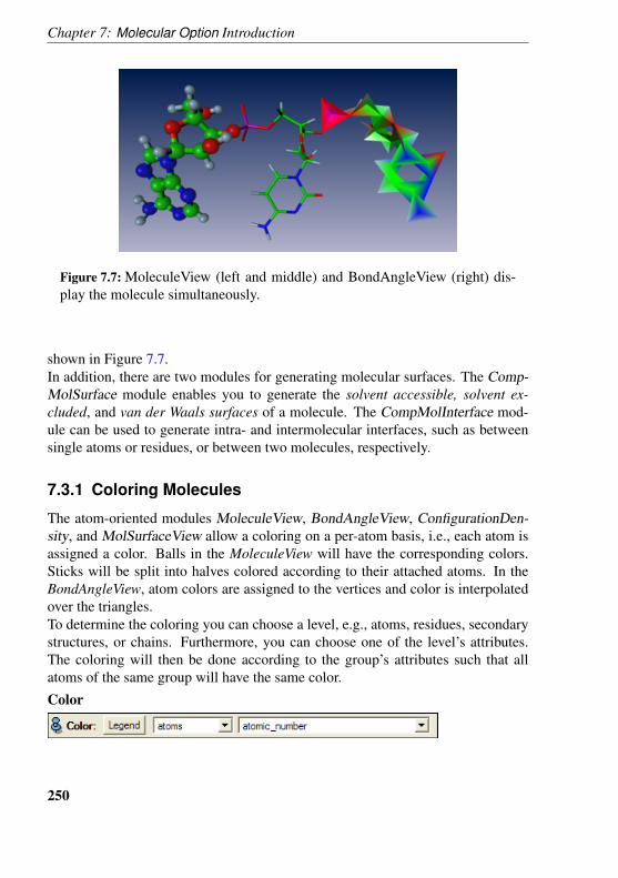
Chapter 7: Molecular Option Introduction
Figure 7.7: MoleculeView (left and middle) and BondAngleView (right) dis-play the molecule simultaneously.
shown in Figure 7.7.In addition, there are two modules for generating molecular surfaces. The Comp-MolSurface module enables you to generate the solvent accessible, solvent ex-cluded, and van der Waals surfaces of a molecule. The CompMolInterface mod-ule can be used to generate intra- and intermolecular interfaces, such as betweensingle atoms or residues, or between two molecules, respectively.
7.3.1 Coloring Molecules
The atom-oriented modules MoleculeView, BondAngleView, ConfigurationDen-sity, and MolSurfaceView allow a coloring on a per-atom basis, i.e., each atom isassigned a color. Balls in the MoleculeView will have the corresponding colors.Sticks will be split into halves colored according to their attached atoms. In theBondAngleView, atom colors are assigned to the vertices and color is interpolatedover the triangles.To determine the coloring you can choose a level, e.g., atoms, residues, secondarystructures, or chains. Furthermore, you can choose one of the level’s attributes.The coloring will then be done according to the group’s attributes such that allatoms of the same group will have the same color.
Color
250
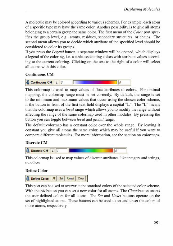
Displaying Molecules
A molecule may be colored according to various schemes. For example, each atomof a specific type may have the same color. Another possibility is to give all atomsbelonging to a certain group the same color. The first menu of the Color port spec-ifies the group level, e.g., atoms, residues, secondary structures, or chains. Thesecond menu allows you to decide which attribute of the specified level should beconsidered to color its groups.If you press the Legend button, a separate window will be opened, which displaysa legend of the coloring, i.e. a table associating colors with attribute values accord-ing to the current coloring. Clicking on the text to the right of a color will selectall atoms with this color.
Continuous CM
This colormap is used to map values of float attributes to colors. For optimalmapping, the colormap range must be set correctly. By default, the range is setto the minimum and maximum values that occur using the chosen color scheme,if the button in front of the first text field displays a capital ”L”. The ”L” meansthat the colormap uses a local range which allows you to modify the range withoutaffecting the range of the same colormap used in other modules. By pressing thebutton you can toggle between local and global range.The default colormap has a constant color over the whole range. By leaving itconstant you give all atoms the same color, which may be useful if you want tocompare different molecules. For more information, see the section on colormaps.
Discrete CM
This colormap is used to map values of discrete attributes, like integers and strings,to colors.
Define Color
This port can be used to overwrite the standard colors of the selected color scheme.With the All button you can set a new color for all atoms. The Clear button unsetsthe user-defined colors for all atoms. The Set and Unset buttons operate on theset of highlighted atoms. These buttons can be used to set and unset the colors ofthose atoms, respectively.
251
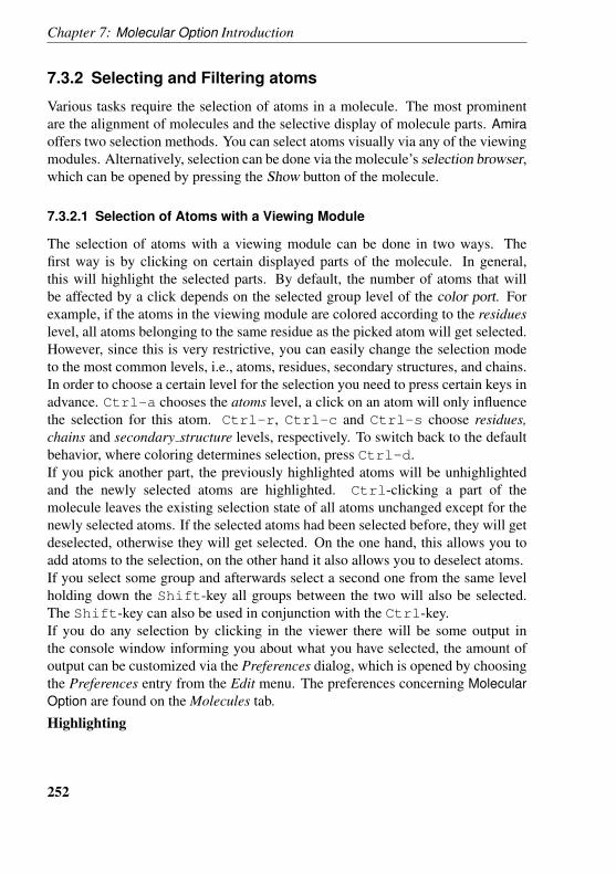
Chapter 7: Molecular Option Introduction
7.3.2 Selecting and Filtering atoms
Various tasks require the selection of atoms in a molecule. The most prominentare the alignment of molecules and the selective display of molecule parts. Amiraoffers two selection methods. You can select atoms visually via any of the viewingmodules. Alternatively, selection can be done via the molecule’s selection browser,which can be opened by pressing the Show button of the molecule.
7.3.2.1 Selection of Atoms with a Viewing Module
The selection of atoms with a viewing module can be done in two ways. Thefirst way is by clicking on certain displayed parts of the molecule. In general,this will highlight the selected parts. By default, the number of atoms that willbe affected by a click depends on the selected group level of the color port. Forexample, if the atoms in the viewing module are colored according to the residueslevel, all atoms belonging to the same residue as the picked atom will get selected.However, since this is very restrictive, you can easily change the selection modeto the most common levels, i.e., atoms, residues, secondary structures, and chains.In order to choose a certain level for the selection you need to press certain keys inadvance. Ctrl-a chooses the atoms level, a click on an atom will only influencethe selection for this atom. Ctrl-r, Ctrl-c and Ctrl-s choose residues,chains and secondary structure levels, respectively. To switch back to the defaultbehavior, where coloring determines selection, press Ctrl-d.If you pick another part, the previously highlighted atoms will be unhighlightedand the newly selected atoms are highlighted. Ctrl-clicking a part of themolecule leaves the existing selection state of all atoms unchanged except for thenewly selected atoms. If the selected atoms had been selected before, they will getdeselected, otherwise they will get selected. On the one hand, this allows you toadd atoms to the selection, on the other hand it also allows you to deselect atoms.If you select some group and afterwards select a second one from the same levelholding down the Shift-key all groups between the two will also be selected.The Shift-key can also be used in conjunction with the Ctrl-key.If you do any selection by clicking in the viewer there will be some output inthe console window informing you about what you have selected, the amount ofoutput can be customized via the Preferences dialog, which is opened by choosingthe Preferences entry from the Edit menu. The preferences concerning MolecularOption are found on the Molecules tab.
Highlighting
252
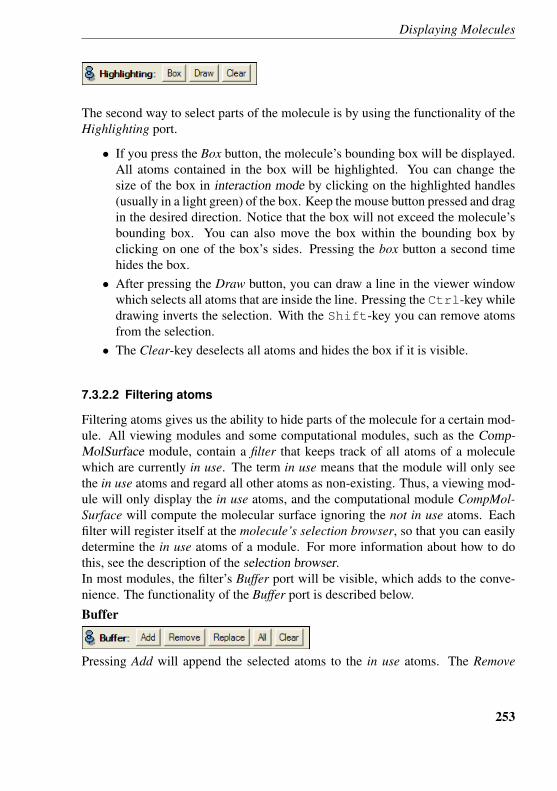
Displaying Molecules
The second way to select parts of the molecule is by using the functionality of theHighlighting port.
• If you press the Box button, the molecule’s bounding box will be displayed.All atoms contained in the box will be highlighted. You can change thesize of the box in interaction mode by clicking on the highlighted handles(usually in a light green) of the box. Keep the mouse button pressed and dragin the desired direction. Notice that the box will not exceed the molecule’sbounding box. You can also move the box within the bounding box byclicking on one of the box’s sides. Pressing the box button a second timehides the box.
• After pressing the Draw button, you can draw a line in the viewer windowwhich selects all atoms that are inside the line. Pressing the Ctrl-key whiledrawing inverts the selection. With the Shift-key you can remove atomsfrom the selection.
• The Clear-key deselects all atoms and hides the box if it is visible.
7.3.2.2 Filtering atoms
Filtering atoms gives us the ability to hide parts of the molecule for a certain mod-ule. All viewing modules and some computational modules, such as the Comp-MolSurface module, contain a filter that keeps track of all atoms of a moleculewhich are currently in use. The term in use means that the module will only seethe in use atoms and regard all other atoms as non-existing. Thus, a viewing mod-ule will only display the in use atoms, and the computational module CompMol-Surface will compute the molecular surface ignoring the not in use atoms. Eachfilter will register itself at the molecule’s selection browser, so that you can easilydetermine the in use atoms of a module. For more information about how to dothis, see the description of the selection browser.In most modules, the filter’s Buffer port will be visible, which adds to the conve-nience. The functionality of the Buffer port is described below.
Buffer
Pressing Add will append the selected atoms to the in use atoms. The Remove
253
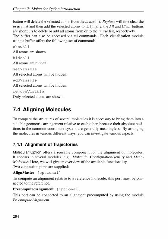
Chapter 7: Molecular Option Introduction
button will delete the selected atoms from the in use list. Replace will first clear thein use list and then add the selected atoms to it. Finally, the All and Clear buttonsare shortcuts to delete or add all atoms from or to the in use list, respectively.The buffer can also be accessed via tcl commands. Each visualization moduleusing a buffer offers the following set of commands:showAll
All atoms are shown.hideAll
All atoms are hidden.setVisible
All selected atoms will be hidden.addVisible
All selected atoms will be hidden.removeVisible
Only selected atoms are shown.
7.4 Aligning Molecules
To compare the structures of several molecules it is necessary to bring them into asuitable geometric arrangement relative to each other, because their absolute posi-tions in the common coordinate system are generally meaningless. By arrangingthe molecules in various different ways, you can investigate various aspects.
7.4.1 Alignment of Trajectories
Molecular Option offers a reusable component for the alignment of molecules.It appears in several modules, e.g., Molecule, ConfigurationDensity and Mean-Molecule. Here, we will give an overview of the available functionality.Two connection ports are supplied:AlignMaster [optional]
To compute an alignment relative to a reference molecule, this port must be con-nected to the reference.PrecomputedAlignment [optional]
This port can be connected to an alignment precomputed by using the modulePrecomputeAlignment.
254
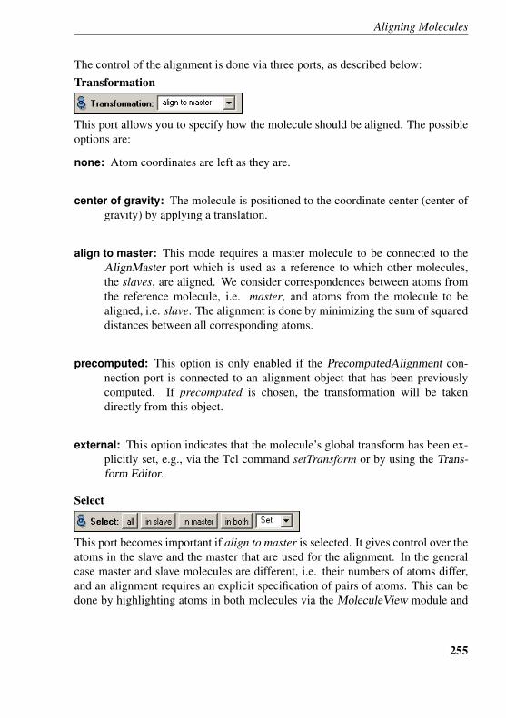
Aligning Molecules
The control of the alignment is done via three ports, as described below:Transformation
This port allows you to specify how the molecule should be aligned. The possibleoptions are:
none: Atom coordinates are left as they are.
center of gravity: The molecule is positioned to the coordinate center (center ofgravity) by applying a translation.
align to master: This mode requires a master molecule to be connected to theAlignMaster port which is used as a reference to which other molecules,the slaves, are aligned. We consider correspondences between atoms fromthe reference molecule, i.e. master, and atoms from the molecule to bealigned, i.e. slave. The alignment is done by minimizing the sum of squareddistances between all corresponding atoms.
precomputed: This option is only enabled if the PrecomputedAlignment con-nection port is connected to an alignment object that has been previouslycomputed. If precomputed is chosen, the transformation will be takendirectly from this object.
external: This option indicates that the molecule’s global transform has been ex-plicitly set, e.g., via the Tcl command setTransform or by using the Trans-form Editor.
Select
This port becomes important if align to master is selected. It gives control over theatoms in the slave and the master that are used for the alignment. In the generalcase master and slave molecules are different, i.e. their numbers of atoms differ,and an alignment requires an explicit specification of pairs of atoms. This can bedone by highlighting atoms in both molecules via the MoleculeView module and
255
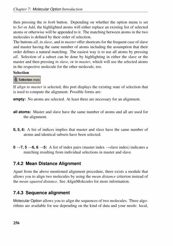
Chapter 7: Molecular Option Introduction
then pressing the in both button. Depending on whether the option menu is setto Set or Add, the highlighted atoms will either replace an existing list of selectedatoms or otherwise will be appended to it. The matching between atoms in the twomolecules is defined by their order of selection.The buttons all, in slave, and in master offer shortcuts for the frequent case of slaveand master having the same number of atoms including the assumption that theirorder defines a natural matching. The easiest way is to use all atoms by pressingall. Selection of a subset can be done by highlighting in either the slave or themaster and then pressing in slave, or in master, which will use the selected atomsin the respective molecule for the other molecule, too.Selection
If align to master is selected, this port displays the existing state of selection thatis used to compute the alignment. Possible forms are:
empty: No atoms are selected. At least three are necessary for an alignment.
all atoms: Master and slave have the same number of atoms and all are used forthe alignment.
0, 5, 6: A list of indices implies that master and slave have the same number ofatoms and identical subsets have been selected.
0→7, 5→6, 6→5: A list of index pairs (master index→slave index) indicates amatching resulting from individual selections in master and slave.
7.4.2 Mean Distance Alignment
Apart from the above mentioned alignment procedure, there exists a module thatallows you to align two molecules by using the mean distance criterion instead ofthe mean squared distance. See AlignMolecules for more information.
7.4.3 Sequence alignment
Molecular Option allows you to align the sequences of two molecules. Three algo-rithms are available for use depending on the kind of data and your needs: local,
256
Visualizing Molecular Trajectories and Metastable Conformations
semi-global, and global alignment. The algorithms work both for proteins andribonucleic acids, whereas t-RNA molecules are currently not supported becausethey contain modified bases. This module can be very helpful when used in con-junction with the AlignMolecules module.
7.5 Visualizing Molecular Trajectories andMetastable Conformations
A MolTrajectory can be visualized via animation of single time steps by attachinga Molecule module to the MolTrajectory and then attaching a MoleculeView orBondAngleView to the Molecule. The animation is controlled via the Molecule’sTime port.For MolTrajectories that represent metastable conformations, the modules Mean-Molecule, PrecomputeAlignment, and ConfigurationDensity can be used. TheMeanMolecule module aligns all steps of a trajectory and computes a meanmolecule by averaging every atomic coordinate over all time steps. Instead ofcomputing the mean molecule to a reference, as with the MeanMolecule module,the PrecomputeAlignment module allows you to find the optimal transformationof each time step to minimize the overall sum of squared distances. With theRankTimeStep module you can search in a trajectory for a desired time step, usingdifferent criteria, such as the rmsd value to a given reference.The ConfigurationDensity module gives an impression of the fuzziness of the con-formation by computing a probability density for the positions of atoms and bondswithin a molecular trajectory. This density can then be visualized with the Isosur-face and Voltex modules.
7.6 Atom Expressions
7.6.1 Overview
Atom expressions are a query language to find and select atoms of certain prop-erties in the molecule for further action. The most important application of atomexpressions in Amira is the highlighting section of the Selection Browser.In Amira, a molecule is separated into groups of different levels. Each group con-tains a set of attributes. (More details of this concept can be found in the descrip-tion of the Attribute Editor). Atom expressions are a simple form of a relational
257
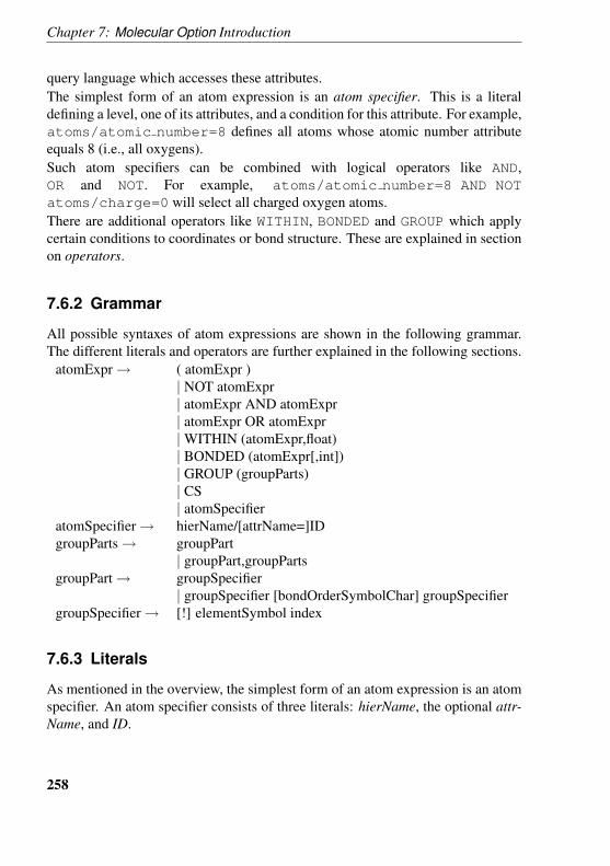
Chapter 7: Molecular Option Introduction
query language which accesses these attributes.The simplest form of an atom expression is an atom specifier. This is a literaldefining a level, one of its attributes, and a condition for this attribute. For example,atoms/atomic number=8 defines all atoms whose atomic number attributeequals 8 (i.e., all oxygens).Such atom specifiers can be combined with logical operators like AND,OR and NOT. For example, atoms/atomic number=8 AND NOTatoms/charge=0 will select all charged oxygen atoms.There are additional operators like WITHIN, BONDED and GROUP which applycertain conditions to coordinates or bond structure. These are explained in sectionon operators.
7.6.2 Grammar
All possible syntaxes of atom expressions are shown in the following grammar.The different literals and operators are further explained in the following sections.
atomExpr→ ( atomExpr )| NOT atomExpr| atomExpr AND atomExpr| atomExpr OR atomExpr|WITHIN (atomExpr,float)| BONDED (atomExpr[,int])| GROUP (groupParts)| CS| atomSpecifier
atomSpecifier→ hierName/[attrName=]IDgroupParts→ groupPart
| groupPart,groupPartsgroupPart→ groupSpecifier
| groupSpecifier [bondOrderSymbolChar] groupSpecifiergroupSpecifier→ [!] elementSymbol index
7.6.3 Literals
As mentioned in the overview, the simplest form of an atom expression is an atomspecifier. An atom specifier consists of three literals: hierName, the optional attr-Name, and ID.
258
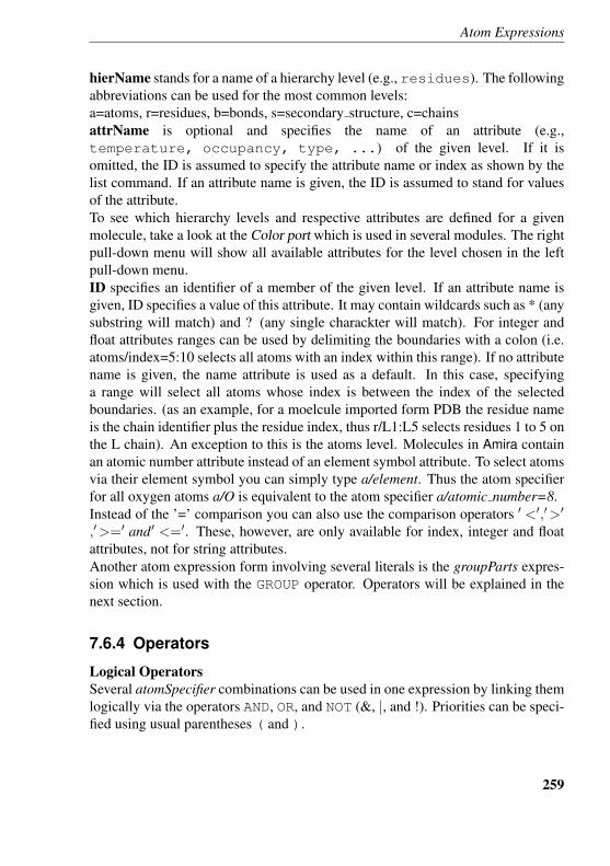
Atom Expressions
hierName stands for a name of a hierarchy level (e.g., residues). The followingabbreviations can be used for the most common levels:a=atoms, r=residues, b=bonds, s=secondary structure, c=chainsattrName is optional and specifies the name of an attribute (e.g.,temperature, occupancy, type, ...) of the given level. If it isomitted, the ID is assumed to specify the attribute name or index as shown by thelist command. If an attribute name is given, the ID is assumed to stand for valuesof the attribute.To see which hierarchy levels and respective attributes are defined for a givenmolecule, take a look at the Color port which is used in several modules. The rightpull-down menu will show all available attributes for the level chosen in the leftpull-down menu.ID specifies an identifier of a member of the given level. If an attribute name isgiven, ID specifies a value of this attribute. It may contain wildcards such as * (anysubstring will match) and ? (any single charackter will match). For integer andfloat attributes ranges can be used by delimiting the boundaries with a colon (i.e.atoms/index=5:10 selects all atoms with an index within this range). If no attributename is given, the name attribute is used as a default. In this case, specifyinga range will select all atoms whose index is between the index of the selectedboundaries. (as an example, for a moelcule imported form PDB the residue nameis the chain identifier plus the residue index, thus r/L1:L5 selects residues 1 to 5 onthe L chain). An exception to this is the atoms level. Molecules in Amira containan atomic number attribute instead of an element symbol attribute. To select atomsvia their element symbol you can simply type a/element. Thus the atom specifierfor all oxygen atoms a/O is equivalent to the atom specifier a/atomic number=8.Instead of the ’=’ comparison you can also use the comparison operators ′ <′,′>′
,′>=′ and′ <=′. These, however, are only available for index, integer and floatattributes, not for string attributes.Another atom expression form involving several literals is the groupParts expres-sion which is used with the GROUP operator. Operators will be explained in thenext section.
7.6.4 Operators
Logical OperatorsSeveral atomSpecifier combinations can be used in one expression by linking themlogically via the operators AND, OR, and NOT (&, |, and !). Priorities can be speci-fied using usual parentheses ( and ).
259
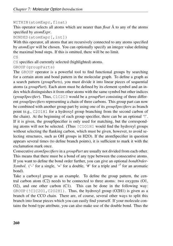
Chapter 7: Molecular Option Introduction
WITHIN(atomExpr,float)This operator selects all atoms which are nearer than float A to any of the atomsspecified by atomExpr.BONDED(atomExpr[,int])With this operator, all atoms that are recursively connected to any atoms specifiedby atomExpr will be chosen. You can optionally specify an integer value definingthe maximal bond steps. If this is omitted, there will be no limit.CSCS specifies all currently selected (highlighted) atoms.GROUP(groupParts)The GROUP operator is a powerful tool to find functional groups by searchingfor a certain atom and bond pattern in the molecular graph. To define a graph asa search pattern (groupParts), you must divide it into linear pieces of sequentialatoms (a groupPart). Each atom must be defined by its element symbol and an in-dex which distinguishes it from other atoms with the same symbol but other indices(groupSpecifier). Thus, C1C2C3 would be a groupPart consisting of three differ-ent groupSpecifiers representing a chain of three carbons. This group part can nowbe combined with another group part by using one of its groupSpecifiers as branchpoint (e.g., C2O1H1 for a hydroxyl group branching from the second carbon ofthe chain). At the beginning of each group specifier, there can be an optional ‘!’.If it is given, the groupSpecifier is only used for matching, but the correspond-ing atoms will not be selected. (Thus !C1O1H1 would find the hydroxyl groupswithout selecting the flanking carbon, which must be given, however, to avoid se-lecting structures, such as OH groups in H2O). If the atomSpecifier in questionappears several times (to define branch points), it is sufficient to mark it with theexclamation mark once.Consecutive atomSpecifiers in a groupPart are usually not divided from each other.This means that there must be a bond of any type between the consecutive atoms.If you want to define the bond order further, you can give an optional bondOrder-Symbol. (‘-’ for a single, ‘=’ for a double, ‘#’ for a triple and ‘’ for an aromaticbond).Take a carboxyl group as an example. To define the group pattern, the cen-tral carbon atom (C2) needs to be connected to three atoms: two oxygens (O1,O2), and one other carbon (C1). This can be done in the following way:GROUP(!C1C2O1,C2O2H1). Thus, the hydroxyl group (O2H1) is given as abranch of the CCO chain. There are, of course, several other ways to split thisbranch into linear pieces which you can easily find yourself. If your molecule con-tains the bond type attribute, you can also make use of the double bond. Thus the
260
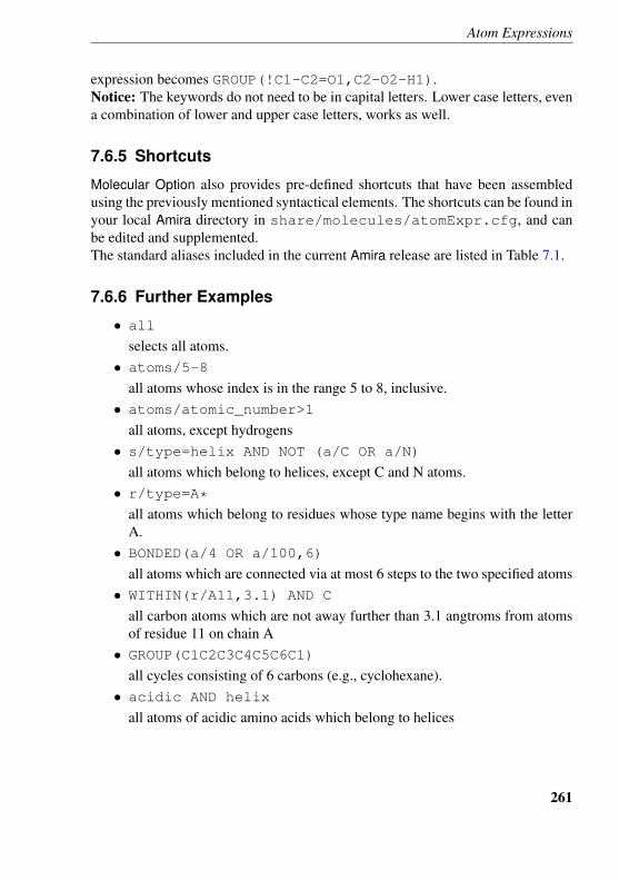
Atom Expressions
expression becomes GROUP(!C1-C2=O1,C2-O2-H1).Notice: The keywords do not need to be in capital letters. Lower case letters, evena combination of lower and upper case letters, works as well.
7.6.5 Shortcuts
Molecular Option also provides pre-defined shortcuts that have been assembledusing the previously mentioned syntactical elements. The shortcuts can be found inyour local Amira directory in share/molecules/atomExpr.cfg, and canbe edited and supplemented.The standard aliases included in the current Amira release are listed in Table 7.1.
7.6.6 Further Examples
• all
selects all atoms.• atoms/5-8
all atoms whose index is in the range 5 to 8, inclusive.• atoms/atomic_number>1
all atoms, except hydrogens• s/type=helix AND NOT (a/C OR a/N)
all atoms which belong to helices, except C and N atoms.• r/type=A*
all atoms which belong to residues whose type name begins with the letterA.
• BONDED(a/4 OR a/100,6)
all atoms which are connected via at most 6 steps to the two specified atoms• WITHIN(r/A11,3.1) AND C
all carbon atoms which are not away further than 3.1 angtroms from atomsof residue 11 on chain A
• GROUP(C1C2C3C4C5C6C1)
all cycles consisting of 6 carbons (e.g., cyclohexane).• acidic AND helix
all atoms of acidic amino acids which belong to helices
261
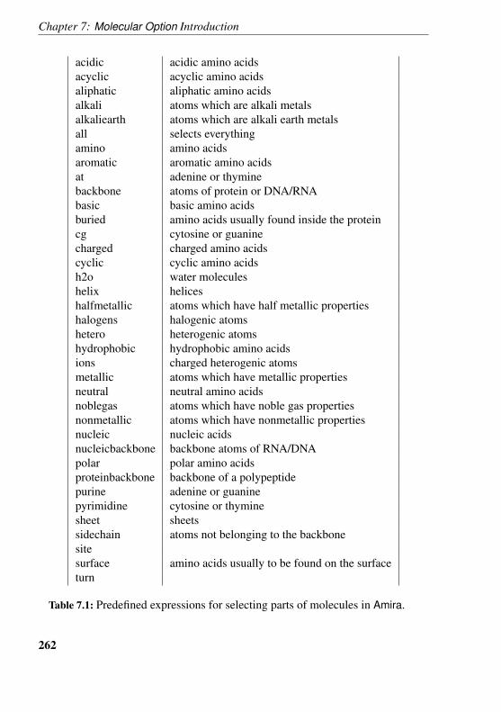
Chapter 7: Molecular Option Introduction
acidic acidic amino acidsacyclic acyclic amino acidsaliphatic aliphatic amino acidsalkali atoms which are alkali metalsalkaliearth atoms which are alkali earth metalsall selects everythingamino amino acidsaromatic aromatic amino acidsat adenine or thyminebackbone atoms of protein or DNA/RNAbasic basic amino acidsburied amino acids usually found inside the proteincg cytosine or guaninecharged charged amino acidscyclic cyclic amino acidsh2o water moleculeshelix heliceshalfmetallic atoms which have half metallic propertieshalogens halogenic atomshetero heterogenic atomshydrophobic hydrophobic amino acidsions charged heterogenic atomsmetallic atoms which have metallic propertiesneutral neutral amino acidsnoblegas atoms which have noble gas propertiesnonmetallic atoms which have nonmetallic propertiesnucleic nucleic acidsnucleicbackbone backbone atoms of RNA/DNApolar polar amino acidsproteinbackbone backbone of a polypeptidepurine adenine or guaninepyrimidine cytosine or thyminesheet sheetssidechain atoms not belonging to the backbonesitesurface amino acids usually to be found on the surfaceturn
Table 7.1: Predefined expressions for selecting parts of molecules in Amira.
262
Part III
Virtual Reality Option User’sGuide
263

8 Virtual Reality Option User’sGuide
The Virtual Reality Option is an Amira extension providing support for large tileddisplays like screen arrays as well as immersive multi-wall displays like CAVEsand Holobenches, with applications ranging from extended resolution displays totrue immersive virtual reality. For performance use of multiple screens or projec-tors, Virtual Reality Option supports either:
• parallel multi-threaded rendering on multi-pipe machines, which are hostingmultiple graphics boards,
• parallel distributed rendering on graphics clusters, which are interconnectedPCs equipped with graphics board (not to be confused with compute clus-ters).
For enhanced interaction and immersion, VR configurations can support activeand passive stereo modes, soft edge blending, head tracking and advanced 3D userinteraction. Any VRCO trackd-compatible tracking system and control devicescan be used together with Virtual Reality Option. Existing Amira modules can bedirectly used in an immersive environment by means of 3D menus. Scripts canbe used for customization. In addition, a simple API is provided, allowing anDeveloper Option programmer to add display modules with a specific interactionbehaviour.The documentation of Virtual Reality Option configurations is separated into thefollowing parts:Configuration and startup
• Virtual Reality Option essentials• Using a multi-pipe system• Using a cluster system• Flat screen configurations• Immersive configurations
265
Chapter 8: Virtual Reality Option User’s Guide
• Calibrating the tracking system
Working with Virtual Reality Option:
• 3D user interaction, including the 3D menu• Writing Virtual Reality Option custom modules
Reference sections
• Config file reference• The AmiraVR control module• The ShowConfig module• The tracker emulator
8.1 Virtual Reality Option Essentials
8.1.1 Virtual Reality Option configurations
Virtual Reality Option can be configured in many differ-ent ways. A particular configuration is described in aconfig file under $AMIRA ROOT/share/config/vr or$AMIRA LOCAL/share/config/vr. The config file contains thingslike the layout or physical extent of the screens of the display system, informationabout the display sources such as the X display or the parts of the desktop mappedonto the screens, as well as optional calibration data for the tracking system.When Virtual Reality Option is installed the Amira main window provides an ad-ditional menu labelled VR. This menu lists all config files found in the configdirectory. Once a particular configuration is selected, the AmiraVR module is cre-ated - if one does not already exists. Depending on the particular configuration theAmiraVR module allows the user to connect to the tracking system, to calibrate thetracking system, or to activate additional options.Configurations are detailed in further sections.
8.1.2 Immersive interaction and the trackd daemon
For immersive displays with head tracking or interaction with 3D input devices,Virtual Reality Option makes use of the VRCO trackd software in order to access
266
Using Virtual Reality Option on a multi-pipe system
the tracking system and controller devices. Trackd itself is not part of Virtual Re-ality Option. For more information about purchasing and installing trackd, pleaserefer to www.vrco.com or 3dviz.mc.com.Before a tracking system can be used in Virtual Reality Option the trackd daemon(and possibly a trackd server) has to be started. The trackd daemon connects to thetracking system and controller device and provides the actual tracker and controllerdata in two shared memory segments, which are read by Amira.
8.1.3 Multiple displays and parallel rendering
Virtual Reality Option can use simple configurations driven by a single graphicsboard, possibly using several video outputs (e.g. dual-head). It also supports con-figurations requiring more outputs than available from a single board (tiled or arbi-trary multi-displays). Having a single screen or projector per graphics board mayalso be preferred for performance. This can be achieved either by using a multi-pipe computer hosting multiple graphics boards (section 8.2), or using a cluster ofcomputers (section 8.3).Virtual Reality Option manages application synchronization and OpenGL framebuffer swap synchronization for all displays, so that the same content can renderedsimultaneously on each display, yet possibly with a different viewpoint.A type of stereoscopic displays relies on active shutter glasses synchronized withthe display, where the left and right eye images are rendered alternatively (OpenGLquadbuffered stereo). Active stereo requires synchronizing the video signals of thewhole graphics boards. This can be achieved for instance with hardware frame-lock/genlock as provided by NVidia ’G’ cards. Passive stereoscopy, for instanceusing polarizing filter glasses, does not require video frame synchronization.
8.2 Using Virtual Reality Option on a multi-pipesystem
8.2.1 Configuration
Effective rendering on a multi-pipe system requires parallel rendering, i.e. send-ing data to the graphics engines from several threads running in parallel. Note thatfor all common current graphics architectures it makes no sense to render multiplewindows on the same pipe in parallel. Typically, this even implies a significant per-formance decrease. Virtual Reality Option configurations allows to define display
267
Chapter 8: Virtual Reality Option User’s Guide
thread groups for multi-pipe rendering (more about configuration with examplesin next sections).
8.2.2 Starting Amira
After Virtual Reality Option has been installed Amira can be started as usual. How-ever, in order to activate parallel rendering of screens assigned to different threadgroups, Amira should be started with the -mt command line options. This optionenables multi-threading. In order to permanently activate multi-threading, the en-vironment variable AMIRA MULTITHREAD can be set. In order to disable multi-threading when AMIRA MULTITHREAD is set, Amira can also be started with the-st command line option (single-threaded mode).Note: On some graphics engines such as SGI Onyx systems there are knownproblems with the OpenGL driver related to the use of texture objects in differ-ent OpenGL contexts. If you are rendering more than one screen on a single pipe,you may define the environment variable AMIRA NO CONTEXT SHARING as aworkaround. This may be fixed by some OS or driver update.
8.3 Using Virtual Reality Option on a cluster
8.3.1 Overview
A graphics cluster consists of multiple computers cluster nodes) connected viaa network. Each computer controls one or more screens of a tiled or multi-walldisplay system. Virtual Reality Option synchronizes the different cluster nodes,ensuring that the same scene is rendered simultaneously from different viewpoints.This cluster support enables distributed parallel rendering. It does not speed upordinary computations by distributing them across multiple nodes of the cluster.Instead, on each cluster node a separate instance of Amira is running, with thecomplete modules network and all data being replicated in cluster’s node memory.Changes of Amira modules made on a master node will be propagated to the slavenodes as lightweight command messages and executed synchronously: thereforethe master and the slaves nodes execute the same processing steps. A specialdaemon running on slave nodes is responsible for starting the Amira instance uponrequests of the master, once a cluster configuration is selected. The 2D mouse or a3D input device can be used to interact with the application on the master node.
268
Using Virtual Reality Option on a cluster
8.3.2 Requirements
• All nodes of the cluster should be of the same type. If different hardware isused, it is possible that the cluster will run out-of-sync for instance becauseof round-off errors.
• Rendering speed is limited by the slowest node of the cluster, including themaster node. Therefore it is recommended that all cluster nodes includingthe master node have the same type of graphics board.
• All nodes of the graphics cluster must be able to communicate with eachother via a TCP/IP connection. A standard 10 Mbit ethernet connectionmay be fast enough, since only synchronization commands are exchanged,rather than images or raw data blocks.
• For active stereoscopy, the graphics cards of the different cluster nodes mustbe genlocked with a genlock cable. Currently only a small number of graph-ics cards (such as WildCat, SUN Zulu, NVidia ’G’ boards) provide genlock-ing. Genlocking ensures that the video refresh cycles are synchronized. Vir-tual Reality Option itself only synchronizes OpenGL buffer swaps. Passivestereoscopy does not require genlocking.
• Installation path and data location.When Amira loads scripts or data below its installation directory, the rel-ative path on the master is ’rooted’ to Amira installation directory onslaves. For instance, /master-path/Amira/data/xxx is translatedinto /slave-path/Amira/data/xxx. However it is highly recom-mended that all data files and scripts have the same absolute file path onall nodes of the cluster. Likewise, Amira should be installed at the same lo-cation on all nodes. For convenience, it is recommended to run Amira froma shared mounted file system. This ensures that the same scripts and configfiles will be used on all cluster nodes.
• On a Linux or UNIX cluster, it is recommended to have a shared home direc-tory. This ensures that some modules have consistent access to preferencessettings stored in .AmiraRegistry.
8.3.3 Preparing cluster slave nodes
Amira requires a daemon process to run on each slave node. This sections explainshow this can be achieved automatically or manually.
269
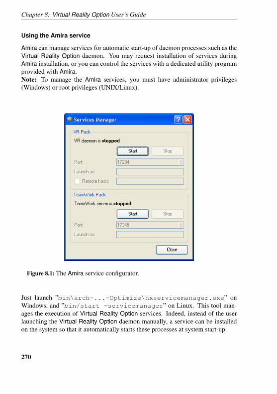
Chapter 8: Virtual Reality Option User’s Guide
Using the Amira service
Amira can manage services for automatic start-up of daemon processes such as theVirtual Reality Option daemon. You may request installation of services duringAmira installation, or you can control the services with a dedicated utility programprovided with Amira.Note: To manage the Amira services, you must have administrator privileges(Windows) or root privileges (UNIX/Linux).
Figure 8.1: The Amira service configurator.
Just launch ”bin\arch-...-Optimize\hxservicemanager.exe” onWindows, and ”bin/start -servicemanager” on Linux. This tool man-ages the execution of Virtual Reality Option services. Indeed, instead of the userlaunching the Virtual Reality Option daemon manually, a service can be installedon the system so that it automatically starts these processes at system start-up.
270
Using Virtual Reality Option on a cluster
In order to install and start a service, click on the Start button. Then, clicking onthe Stop button will stop and uninstall the service.
Platform-dependent notes
• On Windows platforms:Once installed, services can be started or stopped from the services managerof the system that can be launched via the Control Panel (select Administra-tive tools, then Services) or with the command: services.msc /s.
• To start an Amira service, select it in the list (”hxvrdaemon”), thenselect Start from the Action menu.
• To restart the service, select it in the list, then select Restart from theAction menu.
• To stop the service, select it in the list, then select Stop from the Ac-tion menu.
Warning about virtual drives: Amira services do not support log-ical or network volumes. Indeed, such virtual drives do not existin the service execution context. You must specify full paths con-structed according to the universal naming convention (UNC), such as”\\remotemachine\directory”.For example, to install the service from a virtual drive S: targeting adistant mount point ”\\remotemachine\directory”, do not launchthe installer from S:, but from ”\\remotemachine\directory”.Then, for the same reason, the user should not load data from virtual drivesbecause Amira slaves cannot resolve virtual paths unless they are below%AMIRA ROOT%, in which case data paths are re-interpreted on slaves withthe local %AMIRA ROOT%.
• On Unix/Linux platforms:Amira services are implemented as daemons, started from the”/etc/init.d” directory. Once installed, services can be manu-ally started or stopped using the appropriate script. For example, type”/etc/init.d/hxvrdaemon stop” to stop the Virtual RealityOption daemon. Note that this will not uninstall the daemon, that willbe launched on next system start-up (or next ”init 5” mode switch in
271
Chapter 8: Virtual Reality Option User’s Guide
particular).One specific feature of Amira services on Linux platforms is that they canbe executed as a given user, other than root. To do so, just type a valid loginin the user field, then restart the service to take the change into account.One other specific feature is that Virtual Reality Option daemons can beinstalled on remote nodes of a cluster from the master node, provided thefact that %AMIRA ROOT% is the same on every machine. Just type the listof the nodes hostnames separated by space chars. Make sure that ssh isinstalled on all machines and configured to use RSA authentication protocol(public and private key files) so that you will not be prompted for passwordon any operation.
Running the daemon
If the Amira service cannot be used for some reason, one can use manual start-up. On Linux start Amira with command line option -clusterdaemon, onWindows start hxvrdaemon.exeOn Windows, to start the daemon automatically after the computer is booted, ashortcut to the daemon executable can be added to the Start/Programs/Startupfolder.
8.3.4 Running Virtual Reality Option on cluster
The following steps are required to use cluster configurations:
1. Install Virtual Reality Option on every node of the graphics cluster under thesame absolute path name, or better yet, create a mounted file system withthe same absolute path name on every node.
2. Create a standard Virtual Reality Option config file describing the geometryof your display system (see the next sections about configurations). Thenadd a field hostname in each screen section. This field indicates on whichnode the screen will be rendered. The config file must be stored on all nodesin the directory $AMIRA ROOT/share/config/vr.
3. Choose one node as the master node. After Amira installation, a daemon isstarted on the slave nodes, by a service on Windows systems or by inetd onUnix/Linux systems. Start Virtual Reality Option on the master and selectyour cluster configuration from the config menu. Slave instances of VirtualReality Option should now be started on all nodes specified in the config file.
272
Using Virtual Reality Option on a cluster
To use the -clusterdaemon option, stop the daemon (see 8.3.3 service man-agement) and replace step 3 by the following steps:
1. Choose one node as the master node. On all other nodes start Amira with thecommand line option -clusterdaemon. With this option a little daemonis started, to which the master process can talk. The daemon automaticallystarts a slave instance of the real Amira if necessary.
2. Start Virtual Reality Option on the master node. Then select your clusterconfiguration from the config menu. Slave instances of Virtual Reality Op-tion should now be started on all nodes specified in the config file.
3. Next you can load any standard Amira network script. For example, openthe online help browser on the master node and choose one of the standardVirtual Reality Option tracking demos. The particular script will be loadedon all slaves as well. Once a script has been loaded, all standard VirtualReality Option interaction modes are available in cluster mode too.
8.3.5 Limitations
• The primary focus of the Virtual Reality Option cluster version is on work-ing in a VR environment. Consequently all manipulations performed in VRmode, e.g., via the 3D menu, will be properly synchronized. On the otherhand, currently not all manipulations made on the master node via the con-ventional 2D user interface will be synchronized.
• Any kind of 2D mouse interaction in a 3D viewer window also will not besynchronized in cluster mode. Thus you cannot draw a lasso area with the2D mouse. Mouse manipulation and interaction are entirely disabled onslaves nodes.
• Transform editors and clip planes are synchronized in cluster mode, whileother editors may be grayed out and not accessible.
• When loading a new cluster configuration file, Amira attempts to send thecurrent network to slaves nodes for reloading after they are restarted. Datashould be duplicated or shared in order to have the same path relative toscript. This may also fail if default directory for temporary files are not thesame path on master and slaves. You may check TMPDIR, TEMP or TMPenvironment variable depending on your system.
273
Chapter 8: Virtual Reality Option User’s Guide
8.3.6 Troubleshooting cluster configurations
• Check that cluster slaves can be reached from master. ping<slave-hostname> or ping <slave-IP-adress> You canchange hostnames with IP adresses in the configuration file.
• Check that cluster master can be reached from slave with master hostnamewith ping <master-hostname>. Otherwise, on the master node youcan set the environment variable AMIRA HOSTNAME to the master host-name or IP address that can be used from slaves to reach the master.
• Check that Amira runs properly on each slaves. You may need to switchkeyboard and mouse to each slave nodes for checking. You may first tryhint below.
• In order to show and check console output on slaves, you can reduce thechannel size in SoScreen, and add in the configuration file:
SoVRProperty {showSlaveConsole TRUEshowSlaveGUI TRUEshowSlaveCursor TRUE
}
showSlaveCursor should be set if you wish to use a mouse connected to aslave node.
• It is recommended to have one and only one screen defined for the masterin the configuration file (SoScreen without specified hostname). Use SoVR-Property with keepMasterViewerInsideGUI field for convenience.
• Do not mix flat and immersive screen definitions.• Make sure that no firewall limits communication within the cluster (port
17234 and dynamic port are used).
8.4 Flat Screen Configurations
A flat screen configuration consists of usually two or more screens forming a big-ger 2D virtual graphics window commonly called a tiled display or power wall.Users can interact with the ordinary 2D mouse, i.e., mouse events in the differ-ent windows are translated and interpreted in the 2D virtual window. There is
274
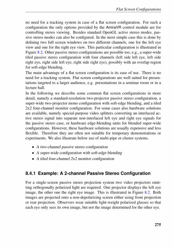
Flat Screen Configurations
no need for a tracking system in case of a flat screen configuration. For such aconfiguration the only options provided by the AmiraVR control module are forcontrolling stereo viewing. Besides standard OpenGL active stereo modes, pas-sive stereo modes can also be configured. In the most simple case this is done bydefining two full screen windows on two different channels, one for the left eyeview and one for the right eye view. This particular configuration is illustrated inFigure 8.2. Other passive stereo configurations are possible too, e.g., a super-widetiled passive stereo configuration with four channels (left side left eye, left sideright eye, right side left eye, right side right eye), possibly with an overlap regionfor soft-edge blending.The main advantage of a flat screen configuration is its ease of use. There is noneed for a tracking system. Flat screen configurations are well suited for presen-tations targeted to a larger audience, e.g. presentations in a seminar room or in alecture hall.In the following we describe some common flat screen configurations in moredetail, namely a standard-resolution two-projector passive stereo configuration, asuper-wide two-projector mono configuration with soft-edge blending, and a tiled2x2 four-channel monitor configuration. For some cases also hardware solutionsare available, namely special-purpose video splitters converting an interlaced ac-tive stereo signal into separate non-interlaced left eye and right eye signals forthe passive stereo case, or hardware edge-blending units for blended super-wideconfigurations. However, these hardware solutions are usually expensive and lessflexible. Therefore they are often not suitable for temporary demonstrations orexperiments. We also illustrate below use of multi-pipe or cluster systems.
• A two-channel passive stereo configuration• A super-wide configuration with soft-edge blending• A tiled four-channel 2x2 monitor configuration
8.4.1 Example: A 2-channel Passive Stereo Configuration
For a single-screen passive stereo projection system two video projectors emit-ting orthogonally polarized light are required. One projector displays the left eyeimage, the other one the right eye image. This is illustrated in Figure 8.2. Bothimages are projected onto a non-depolarizing screen either using front projectionor rear projection. Observers wear suitable light-weight polarized glasses so thateach eye only sees its own image, but not the image determined for the other eye.
275
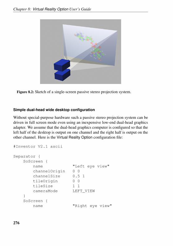
Chapter 8: Virtual Reality Option User’s Guide
Figure 8.2: Sketch of a single-screen passive stereo projection system.
Simple dual-head wide desktop configuration
Without special-purpose hardware such a passive stereo projection system can bedriven in full screen mode even using an inexpensive low-end dual-head graphicsadapter. We assume that the dual-head graphics computer is configured so that theleft half of the desktop is output on one channel and the right half is output on theother channel. Here is the Virtual Reality Option configuration file:
#Inventor V2.1 ascii
Separator {SoScreen {
name "Left eye view"channelOrigin 0 0channelSize 0.5 1tileOrigin 0 0tileSize 1 1cameraMode LEFT_VIEW
}SoScreen {
name "Right eye view"
276
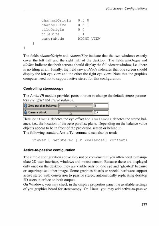
Flat Screen Configurations
channelOrigin 0.5 0channelSize 0.5 1tileOrigin 0 0tileSize 1 1cameraMode RIGHT_VIEW
}}
The fields channelOrigin and channelSize indicate that the two windows exactlycover the left half and the right half of the desktop. The fields tileOrigin andtileSize indicate that both screens should display the full viewer window, i.e., thereis no tiling at all. Finally, the field cameraMode indicates that one screen shoulddisplay the left eye view and the other the right eye view. Note that the graphicscomputer need not to support active stereo for this configuration.
Controlling stereoscopy
The AmiraVR module provides ports in order to change the default stereo parame-ters eye offset and stereo balance.
Here <offset> denotes the eye offset and <balance> denotes the stereo bal-ance, i.e., the location of the zero parallax plane. Depending on the balance valueobjects appear to be in front of the projection screen or behind it.The following standard Amira Tcl command can also be used:
viewer 0 setStereo [-b <balance>] <offset>
Active-to-passive configuration
The simple configuration above may not be convenient if you often need to manip-ulate 2D user interface, windows and mouse cursor. Because these are displayedonly once on the desktop, they are visible only on one eye and ’ghosted’ becauseor superimposed other image. Some graphics boards or special hardware supportactive stereo with conversion to passive stereo, automatically replicating desktop2D users interface on both outputs.On Windows, you may check in the display properties panel the available settingsof you graphics board for stereoscopy. On Linux, you may add active-to-passive
277
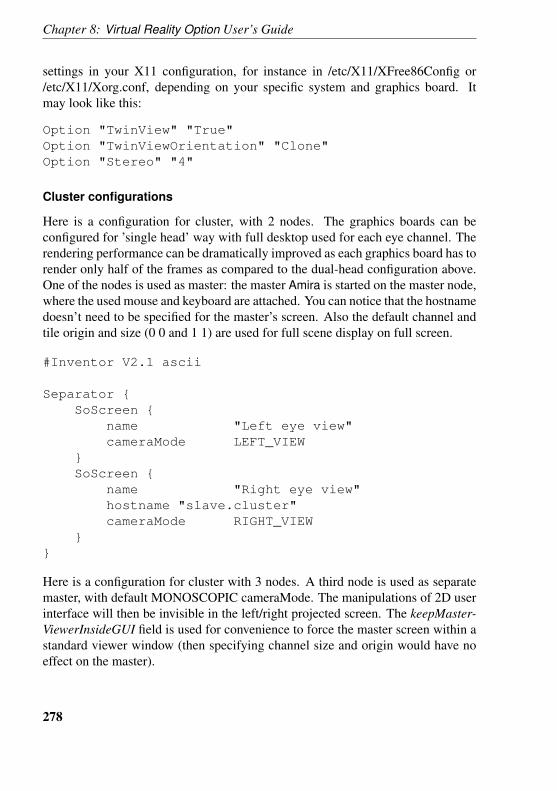
Chapter 8: Virtual Reality Option User’s Guide
settings in your X11 configuration, for instance in /etc/X11/XFree86Config or/etc/X11/Xorg.conf, depending on your specific system and graphics board. Itmay look like this:
Option "TwinView" "True"Option "TwinViewOrientation" "Clone"Option "Stereo" "4"
Cluster configurations
Here is a configuration for cluster, with 2 nodes. The graphics boards can beconfigured for ’single head’ way with full desktop used for each eye channel. Therendering performance can be dramatically improved as each graphics board has torender only half of the frames as compared to the dual-head configuration above.One of the nodes is used as master: the master Amira is started on the master node,where the used mouse and keyboard are attached. You can notice that the hostnamedoesn’t need to be specified for the master’s screen. Also the default channel andtile origin and size (0 0 and 1 1) are used for full scene display on full screen.
#Inventor V2.1 ascii
Separator {SoScreen {
name "Left eye view"cameraMode LEFT_VIEW
}SoScreen {
name "Right eye view"hostname "slave.cluster"cameraMode RIGHT_VIEW
}}
Here is a configuration for cluster with 3 nodes. A third node is used as separatemaster, with default MONOSCOPIC cameraMode. The manipulations of 2D userinterface will then be invisible in the left/right projected screen. The keepMaster-ViewerInsideGUI field is used for convenience to force the master screen within astandard viewer window (then specifying channel size and origin would have noeffect on the master).
278
Flat Screen Configurations
#Inventor V2.1 ascii
Separator {SoVRProperty {
keepMasterViewerInsideGUI TRUE}SoScreen {
name "Master view"}SoScreen {
name "Left eye view"hostname "slave1.cluster"cameraMode LEFT_VIEW
}SoScreen {
name "Right eye view"hostname "slave2.cluster"cameraMode RIGHT_VIEW
}}
8.4.2 Example: A Super-wide Configuration with Soft-edgeBlending
Super-wide images with two times a standard monitor’s resolution can be dis-played using two projectors and a low-end dual-head graphics adapter. However,often it is very desirable to have an overlap between the two projected images inorder to hide at best the transition between the projected images. In the overlap re-gion one image softly fades out from full intensity to black, while the other imagefades in from black to full intensity. This technique is called soft-edge blending(compare Figure 8.3). With soft-edge blending the border between the two pro-jected images becomes almost invisible. Virtual Reality Option is able to generatetwo partially overlapping images. In addition, the soft-edge can be computed insoftware, yet some projectors or external blending units support this directly inhardware. With these features perfect full-screen demos can be presented on asuper-wide projection system.
279
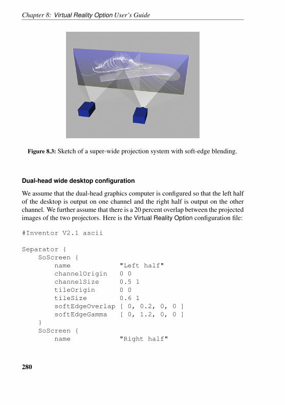
Chapter 8: Virtual Reality Option User’s Guide
Figure 8.3: Sketch of a super-wide projection system with soft-edge blending.
Dual-head wide desktop configuration
We assume that the dual-head graphics computer is configured so that the left halfof the desktop is output on one channel and the right half is output on the otherchannel. We further assume that there is a 20 percent overlap between the projectedimages of the two projectors. Here is the Virtual Reality Option configuration file:
#Inventor V2.1 ascii
Separator {SoScreen {
name "Left half"channelOrigin 0 0channelSize 0.5 1tileOrigin 0 0tileSize 0.6 1softEdgeOverlap [ 0, 0.2, 0, 0 ]softEdgeGamma [ 0, 1.2, 0, 0 ]
}SoScreen {
name "Right half"
280
Flat Screen Configurations
channelOrigin 0.5 0channelSize 0.5 1tileOrigin 0.4 0tileSize 0.6 1softEdgeOverlap [ 0.2, 0, 0, 0 ]softEdgeGamma [ 0, 1.2, 0, 0 ]
}}
The fields channelOrigin and channelSize indicate that the two windows exactlycover the left half and the right half of the desktop. The fields tileOrigin andtileSize indicate that both screens display an area of 0.6 times the width of the fulltiled window. The first screen displays the left half of that window, the secondscreen displays the right half.
How to compute tileOrigin and tileSize fields ?
The fields tileOrigin and tileSize define to the portion of the full view volume, i.e.of the total virtual big screen, to be mapped onto a specific screen. Therefore,if width is the pixel width of one projector, overlap the amount of overlappingpixels, and n the number of projectors, the total pixel width of the screen is:total = (width - overlap)*(n-1) + widthThen:tileSize x = width / totaltileOrigin x = screen-index * (width - overlap) / total
Soft-edge blending fields
The field softEdgeOverlap specifies the relative width of the soft-edge region atthe left, right, bottom, and top border of the screen. For the first screen there is a20 percent soft-edge region at the right border, for the second screen there is a 20percent soft-edge region at the left border.Finally, the field softEdgeGamma specifies the gamma factor for the soft-edgeregion. The gamma factor determines how the fading from full intensity to blackis done. A gamma factor of one means a linear transition in terms of RGB values.However, since RGB values are usually not mapped linearly to light intensity bythe video projector often a decrease of overall light intensity is observed in the
281
Chapter 8: Virtual Reality Option User’s Guide
overlap region. In order to compensate for this a gamma factor larger than one canbe used.In order to facilitate the initial calibration of a super-wide projection system withsoft-edge blending the AmiraVR module provides a special-purpose Tcl commandsetSoftEdge. This command is used in the following way:
VRSettings setSoftEdge -g <gamma> <overlap> [<overlap>...]
This command automatically creates a two-screen configuration similar to the oneabove. However, the correct values for tileSize, tileOrigin, and softEdgeOverlapare computed automatically from the relative overlap value. By gradually adaptingthis value the correct settings for a given but unknown setup of the projectionsystem can be easily found.
Curved screen displays
Tiled display configurations are most often fine for curved displays, which are thenhandled like flat displays. Immersive display configuration fitting the actual screengeometry is required for using stereo with head tracking. Projection onto cylindri-cal or semi-spherical surfaces may also introduce some barrel-shaped distortions.Some special warping hardware can compensate such distortion.
8.4.3 Example: A Tiled 4-channel 2x2 Monitor Configuration
There are some interesting graphics workstations with two two-channel graphicspipes. One example is the SGI Octane Fuel. With such a computer four differentmonitors or projectors can be used. For some purposes it is useful to have a sin-gle viewer subdivided into 2x2 parts and each part being displayed by a differentmonitor. Such a configuration can be easily created using Virtual Reality Option.We assume that the graphics computer has two pipes with two channels each. Thetwo pipes are configured as two separate X11 screens, :0.0 and :0.1. The leftand right part of each screen is output on the two different channels of the particularpipe. Then the configuration files looks as follows:
#Inventor V2.1 ascii
Separator {SoScreen {
name "Upper left monitor"
282
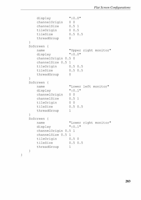
Flat Screen Configurations
display ":0.0"channelOrigin 0 0channelSize 0.5 1tileOrigin 0 0.5tileSize 0.5 0.5threadGroup 0
}SoScreen {
name "Upper right monitor"display ":0.0"channelOrigin 0.5 0channelSize 0.5 1tileOrigin 0.5 0.5tileSize 0.5 0.5threadGroup 0
}SoScreen {
name "Lower left monitor"display ":0.1"channelOrigin 0 0channelSize 0.5 1tileOrigin 0 0tileSize 0.5 0.5threadGroup 1
}SoScreen {
name "Lower right monitor"display ":0.1"channelOrigin 0.5 1channelSize 0.5 1tileOrigin 0.5 0tileSize 0.5 0.5threadGroup 1
}}
283
Chapter 8: Virtual Reality Option User’s Guide
Multi-pipe rendering
Since the two X11 screens :0.0 and :0.1 are driven by two independent graph-ics pipes it makes sense to perform the rendering on these pipes in parallel. Thisis done by assigning the corresponding screens two different thread groups.
• Note that for all common current graphics architectures it makes no sense torender multiple windows on the same pipe in parallel. Typically, this evenimplies a significant performance decrease. Therefore, here we use only twothread groups instead of four.
• In order to actually activate parallel rendering Amira must be started withthe command line option -mt. Alternatively, the environment variableAMIRA MULTITHREAD can be defined.
8.5 Immersive Configurations
In Virtual Reality Option an immersive configuration differs from a flat screen con-figuration mainly in the way the screens are described in the config file. Whilefor a flat screen configuration it was sufficient to specify which part of a big 2Dvirtual screen was covered by each screen, for an immersive configuration the truephysical coordinates of the screens have to be specified. Knowing the exact spa-tial arrangements of the screens has the advantage that correct perspective viewscan be computed for all screens, provided the 3D position of the observer is alsoknown. In particular, the different screens no longer need to be arranged in a plane.Instead, the screens might be arranged perpendicular to each other like in a CAVEor on a Holobench. In fact, Virtual Reality Option supports any other oblique ar-rangement as well.Since the 3D position of the observer need to be known in order to compute correctperspective views, usually the observer’s eye position is tracked in an immersiveenvironment. In Virtual Reality Option this so-called head tracking can be achievedusing a variety of different tracking systems. Instead of accessing the trackingsystem directly an intermediate software layer is used, namely the trackd softwareof VRCO. trackd runs as a server, communicates with the tracking system, andstores the tracking data in a shared-memory areas which then is read by VirtualReality Option. Using a second sensor not only the observer’s eye position can betracked, but also the position of a virtual wand, i.e., a kind of pointing or interactiondevice to be held in a hand. For large planar screen configurations it sometimesalso makes sense to use a virtual wand without head tracking. The images then
284
Immersive Configurations
will always be computed for a fixed observer’s eye position and possible imageflicker due to noise in the tracking data is avoided, which is an advantage for 3Ddemonstrations in front of a larger audience.Obviously, immersive configurations are more difficult to setup than flat screenconfigurations. Besides defining a suitable Virtual Reality Option configurationfile, also the tracking system and the trackd daemon have to be properly initial-ized. Finally, the tracking system has to be calibrated for use with Virtual RealityOption. In the following sections we first want to present some example configfiles for common immersive environments. In particular config files for a single-wall workbench, for a double-wall Holobench, and for a four-sided CAVE shallbe discussed. The process of calibrating the tracking system and customizing 3Duser interaction is described in subsequent sections.
• A Workbench configuration• A Holobench configuration• A CAVE configuration
8.5.1 Example: A Workbench Configuration
A single-screen 3D projection system is often called an immersive workbench.The actual projection screen can either be in up-right position, or it can be orientedlike the surface of a table. Of course, any other orientation is possible too. Thereare even devices like the Barco Baron with can be arbitrarily tilted between fullyhorizontal and fully vertical position. For Virtual Reality Option there is no dif-ference between these configurations, as long as the tracking system is calibratedin the right way. Traditionally a workbench is driven by a CRT projector usingactive stereo. However, today also passive stereo systems based on two LCD orDLP projectors become more common. In the config file below we assume thatan active stereo system is used, or that a passive stereo system is connected via anappropriate signal splitter. This means that the workbench can be used with anystandard stereo-capable graphics computer. No dual-head or multi-pipe computeris necessary. An example of a single-screen workbench is shown in Figure 8.4.An Virtual Reality Option config file for driving a single-screen immersive work-bench with a tracked 3D input device but without head tracking is listed below.Instead of actually tracking the observer’s eye position in this case a fixed defaultcamera position is used. This can be useful for demonstrations in front of small ormedium-size groups, since it produces less fidget images. In addition, it saves asecond sensor for the tracking system.
285
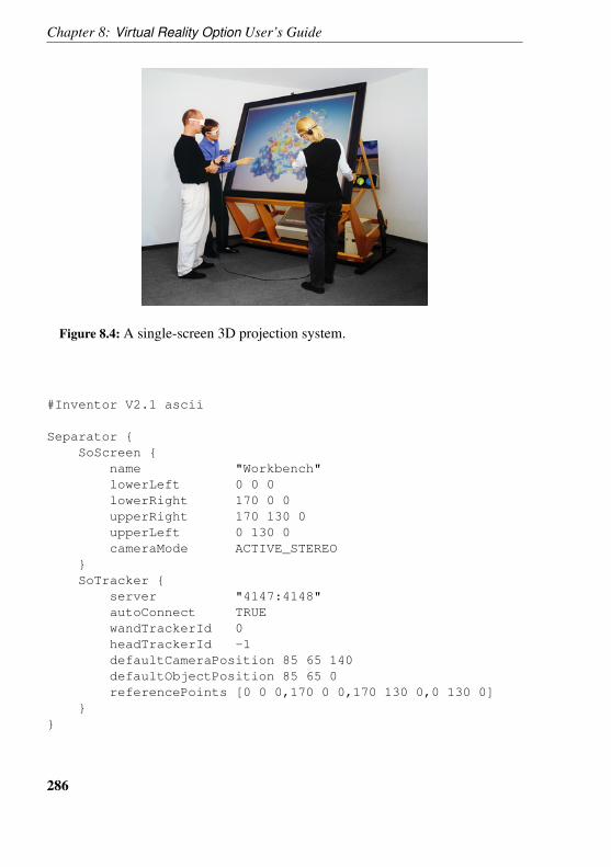
Chapter 8: Virtual Reality Option User’s Guide
Figure 8.4: A single-screen 3D projection system.
#Inventor V2.1 ascii
Separator {SoScreen {
name "Workbench"lowerLeft 0 0 0lowerRight 170 0 0upperRight 170 130 0upperLeft 0 130 0cameraMode ACTIVE_STEREO
}SoTracker {
server "4147:4148"autoConnect TRUEwandTrackerId 0headTrackerId -1defaultCameraPosition 85 65 140defaultObjectPosition 85 65 0referencePoints [0 0 0,170 0 0,170 130 0,0 130 0]
}}
286
Immersive Configurations
Single screen configuration
In the SoScreen section of the config file the physical coordinates of the four cor-ners of the workbench are defined. This can be done using an arbitrary right-handed coordinate system with arbitrary units. In this case the coordinates mightbe specified in centimeters. The origin of the coordinate system was chosen inthe lower left corner of the screen. By default, a full-screen graphics window isopened when activating this configuration. The field cameraMode indicates thatthe graphics window should be opened in active stereo mode by default.
Tracking system configuration
In the SoTracker section of the config file the tracking system is described. Firstthe shared memory ids of the trackd daemon as specified in the trackd.conf file arelisted.The syntax is Id-of-controller-reader:Id-of-tracker-reader.For more information about setting up trackd please refer to section 8.6. The auto-Connect field indicates that a connection to the trackd server should be establishedautomatically as soon as the configuration is activated. wandTrackerId denotes thetrackd sensor id of the 3D input device. Head tracking is disabled by setting head-TrackerId to -1. Instead the default camera position set in the line below is used.This position must be specified using the same coordinate system as the screen. Inthis case the camera is located 140 cm in front of the screen’s center. The defaultobject position is the position where the scene is placed by default (or whenever aview all request comes from the viewer).At the end of the config file four reference points are specified, namely the fourcorners of the screen. Before the configuration can be actually used, the trackingsystem has to be calibrated (see section 8.6). This is done by placing the inputdevice at the reference points and clicking an input button. Once the trackingsystem is calibrated, the config file should be written by clicking the write configbutton of the AmiraVR control module. The new config file will contain the sameinformation listed above, but in addition it will also contain some calibration data,e.g., the transformation between raw tracker coordinates and screen coordinates.
8.5.2 Example: A Holobench Configuration
A Holobench (TM) - or dual-screen workbench - is a special display system con-sisting of two screens oriented perpendicular to each other. One screen is oriented
287
Chapter 8: Virtual Reality Option User’s Guide
vertically, the other one is oriented horizontally like a table. This provides a widefield display with more space free for hand interaction and manipulation as com-pared to a single-screen display. On a good Holobench there is almost no visibleborder between the two screens. Provided the observer’s eye position is known,correct perspective views can be computed so that the displayed scene finally doesnot appear to have any break. However, in contrast to a single-screen workbenchthis is only the case for the tracked observer. Other spectators will more or lessclearly notice a break.In order to drive a workbench at least a stereo-capable dual-head graphics com-puter is required. In principle, two different settings are possible. Either, there is abig desktop and one half of it is output on a first channel and the other one is out-put on a second channel. Or, there are two independent graphics adapters (pipes)which are configured as two different X11 displays or as one display with twoX11 screens. In the config file below we assume, that the desktop is split into twohalves (left and right). An example of how to use a multi-pipe graphics computeris presented in the next section where a 4-sided CAVE configuration is described.
#Inventor V2.1 ascii
Separator {SoScreen {
name "Vertical Screen"lowerLeft 0 0 0lowerRight 180 0 0upperRight 180 110 0upperLeft 0 110 0channelOrigin 0 0channelSize 0.5 1cameraMode ACTIVE_STEREO
}SoScreen {
name "Horizontal Screen (rotated)"lowerLeft 180 0 0lowerRight 0 0 0upperRight 0 0 110upperLeft 180 0 110channelOrigin 0.5 0channelSize 0.5 1cameraMode ACTIVE_STEREO
}
288
Immersive Configurations
SoTracker {server "4147:4148"autoConnect TRUEwandTrackerId 1headTrackerId 0leftEyeOffset 6 0 0rightEyeOffset 13 0 0defaultCameraPosition 90 55 110defaultObjectPosition 90 20 20referencePoints [60 0 110,120 0 110,120 0 55,60 0 55]
}}
Display configuration
In the two SoScreen sections of the config file the geometry of the Holobenchis described by specifying the physical coordinates of the four corners of eachscreen. An arbitrary right-handed coordinate system with arbitrary units can bechosen. Here the coordinates are specified in centimetres and the origin was putin the lower left corner of the vertical screen. Notice, that the horizontal screenwas rotated by 180 degrees with respect to the vertical screen. I.e., instead of theupper left corner the lower right corner of the horizontal screen is located at theorigin. This is because the horizontal image of a Holobench is usually projectedthat way. If the corresponding lower scan-lines of the two images meet at theborder between the two screens artifacts due to delayed response of the activeshutter glasses are avoided. The fields channelOrigin and channelSize indicatethat the graphics window for the vertical screen should be opened on the left halfof the desktop, while the graphics window for the horizontal screen should beopened on the right half. Both windows are opened in stereo mode by default asspecified by cameraMode.
Tracking system configuration
In the SoTracker section of the config file the tracking system is described. Firstthe shared memory ids of the trackd daemon as specified in the trackd.conf file arelisted.The syntax is Id-of-controller-reader:Id-of-tracker-reader.For more information about setting up trackd please refer to section 8.6. TheautoConnect field indicates that a connection to the trackd daemon should be es-
289
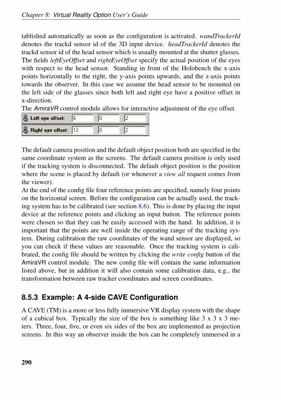
Chapter 8: Virtual Reality Option User’s Guide
tablished automatically as soon as the configuration is activated. wandTrackerIddenotes the trackd sensor id of the 3D input device. headTrackerId denotes thetrackd sensor id of the head sensor which is usually mounted at the shutter glasses.The fields leftEyeOffset and rightEyeOffset specify the actual position of the eyeswith respect to the head sensor. Standing in front of the Holobench the x-axispoints horizontally to the right, the y-axis points upwards, and the z-axis pointstowards the observer. In this case we assume the head sensor to be mounted onthe left side of the glasses since both left and right eye have a positive offset inx-direction.The AmiraVR control module allows for interactive adjustment of the eye offset.
The default camera position and the default object position both are specified in thesame coordinate system as the screens. The default camera position is only usedif the tracking system is disconnected. The default object position is the positionwhere the scene is placed by default (or whenever a view all request comes fromthe viewer).At the end of the config file four reference points are specified, namely four pointson the horizontal screen. Before the configuration can be actually used, the track-ing system has to be calibrated (see section 8.6). This is done by placing the inputdevice at the reference points and clicking an input button. The reference pointswere chosen so that they can be easily accessed with the hand. In addition, it isimportant that the points are well inside the operating range of the tracking sys-tem. During calibration the raw coordinates of the wand sensor are displayed, soyou can check if these values are reasonable. Once the tracking system is cali-brated, the config file should be written by clicking the write config button of theAmiraVR control module. The new config file will contain the same informationlisted above, but in addition it will also contain some calibration data, e.g., thetransformation between raw tracker coordinates and screen coordinates.
8.5.3 Example: A 4-side CAVE Configuration
A CAVE (TM) is a more or less fully immersive VR display system with the shapeof a cubical box. Typically the size of the box is something like 3 x 3 x 3 me-ters. Three, four, five, or even six sides of the box are implemented as projectionscreens. In this way an observer inside the box can be completely immersed in a
290
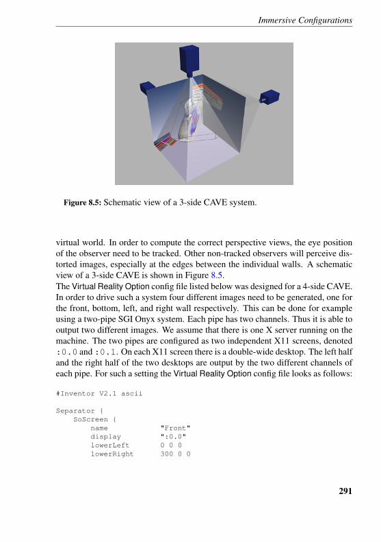
Immersive Configurations
Figure 8.5: Schematic view of a 3-side CAVE system.
virtual world. In order to compute the correct perspective views, the eye positionof the observer need to be tracked. Other non-tracked observers will perceive dis-torted images, especially at the edges between the individual walls. A schematicview of a 3-side CAVE is shown in Figure 8.5.The Virtual Reality Option config file listed below was designed for a 4-side CAVE.In order to drive such a system four different images need to be generated, one forthe front, bottom, left, and right wall respectively. This can be done for exampleusing a two-pipe SGI Onyx system. Each pipe has two channels. Thus it is able tooutput two different images. We assume that there is one X server running on themachine. The two pipes are configured as two independent X11 screens, denoted:0.0 and :0.1. On each X11 screen there is a double-wide desktop. The left halfand the right half of the two desktops are output by the two different channels ofeach pipe. For such a setting the Virtual Reality Option config file looks as follows:
#Inventor V2.1 ascii
Separator {SoScreen {
name "Front"display ":0.0"lowerLeft 0 0 0lowerRight 300 0 0
291
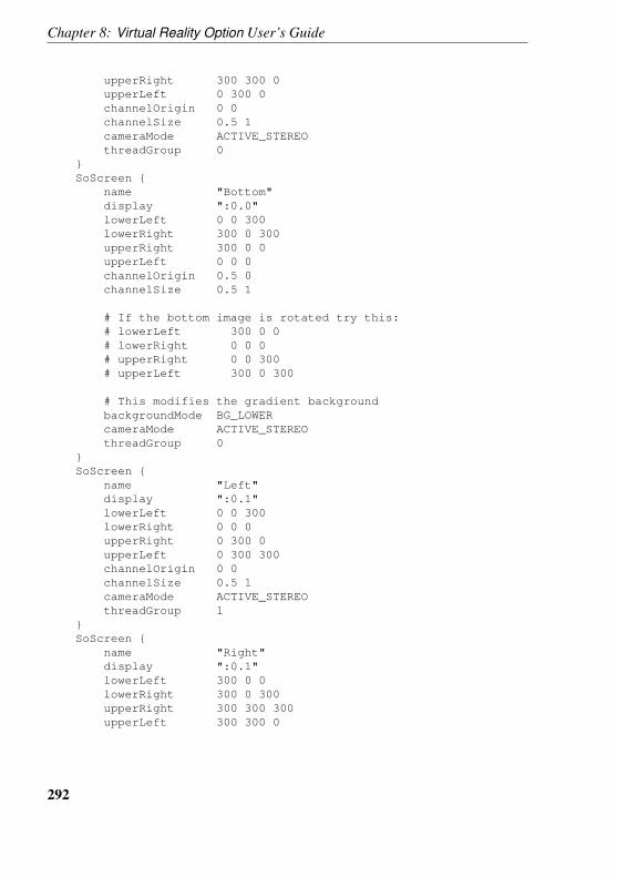
Chapter 8: Virtual Reality Option User’s Guide
upperRight 300 300 0upperLeft 0 300 0channelOrigin 0 0channelSize 0.5 1cameraMode ACTIVE_STEREOthreadGroup 0
}SoScreen {
name "Bottom"display ":0.0"lowerLeft 0 0 300lowerRight 300 0 300upperRight 300 0 0upperLeft 0 0 0channelOrigin 0.5 0channelSize 0.5 1
# If the bottom image is rotated try this:# lowerLeft 300 0 0# lowerRight 0 0 0# upperRight 0 0 300# upperLeft 300 0 300
# This modifies the gradient backgroundbackgroundMode BG_LOWERcameraMode ACTIVE_STEREOthreadGroup 0
}SoScreen {
name "Left"display ":0.1"lowerLeft 0 0 300lowerRight 0 0 0upperRight 0 300 0upperLeft 0 300 300channelOrigin 0 0channelSize 0.5 1cameraMode ACTIVE_STEREOthreadGroup 1
}SoScreen {
name "Right"display ":0.1"lowerLeft 300 0 0lowerRight 300 0 300upperRight 300 300 300upperLeft 300 300 0
292
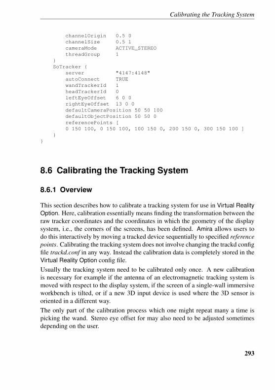
Calibrating the Tracking System
channelOrigin 0.5 0channelSize 0.5 1cameraMode ACTIVE_STEREOthreadGroup 1
}SoTracker {
server "4147:4148"autoConnect TRUEwandTrackerId 1headTrackerId 0leftEyeOffset 6 0 0rightEyeOffset 13 0 0defaultCameraPosition 50 50 100defaultObjectPosition 50 50 0referencePoints [0 150 100, 0 150 100, 100 150 0, 200 150 0, 300 150 100 ]
}}
8.6 Calibrating the Tracking System
8.6.1 Overview
This section describes how to calibrate a tracking system for use in Virtual RealityOption. Here, calibration essentially means finding the transformation between theraw tracker coordinates and the coordinates in which the geometry of the displaysystem, i.e., the corners of the screens, has been defined. Amira allows users todo this interactively by moving a tracked device sequentially to specified referencepoints. Calibrating the tracking system does not involve changing the trackd configfile trackd.conf in any way. Instead the calibration data is completely stored in theVirtual Reality Option config file.Usually the tracking system need to be calibrated only once. A new calibrationis necessary for example if the antenna of an electromagnetic tracking system ismoved with respect to the display system, if the screen of a single-wall immersiveworkbench is tilted, or if a new 3D input device is used where the 3D sensor isoriented in a different way.The only part of the calibration process which one might repeat many a time ispicking the wand. Stereo eye offset for may also need to be adjusted sometimesdepending on the user.
293
Chapter 8: Virtual Reality Option User’s Guide
Wand offset
Picking the wand means to specify the offset between the actual position of the3D input device and the visual representation of the wand in Amira. Sometimes itis useful not to have any offset, while sometimes an offset provides more pleasantand less exhausting working conditions. The wand offset can be quickly adaptedeven multiple times within a single Virtual Reality Option session.
Eye offset
Eye offset for stereoscopy can be defined in the configuration file. It is not amandatory step of the interactive calibration process described below. Howeverthe AmiraVR control module allows for eye offset adjustment at any time (if stereois enabled), and you can then save the configuration.
8.6.2 Tracking system essentials
Before starting calibration make sure that you have a valid Virtual Reality Optionconfig file for your particular display system (you may test it independently fromtracking system). Also make sure that the trackd software and the tracking systemitself are setup in the right way.
Troubleshooting the tracker
A number of factors can affect the tracking system and the returned sensors co-ordinates, and should be kept in mind when calibrating and using Virtual RealityOption, in particular for choosing the reference points used for calibration. Here issummary of the most common possible issues:
• Range. Symptom: instable or wrong tracker coordinates.The calibration reference points or working area may be too far away orhidden from the tracking system. You may check the physical range of yourdevice. You may need to choose reference points closer to tracker, or off thescreen(s), for instance using ruler to offset in front of the screen.
• Hemisphere. Symptom: mirrored coordinates along one axis, reversed rota-tions after calibrationYou should make sure that the tracker coordinates are reported in a right-handed coordinate system. Many electromagnetic tracking systems cannotdistinguish between two opposite hemispheres. In the trackd.conf file you
294
Calibrating the Tracking System
have to specify in which hemisphere you want to operate (e.g. +x, -z..., rel-ative to emitter antenna orientation). If the wrong hemisphere is specified aleft-handed coordinate system is used, which cannot be correctly calibratedin Amira.
• Magnetic perturbation. Symptom: instable/wrong coordinates.With electro-magnetic tracking systems you should avoid calibrating andworking too close to metallic parts such as ferro-magnetic screen frames orsources of magnetic fields such as CRT display monitors. You may need tooffset reference points off the screen.
• Acoustic perturbation. Symptom: instable/wrong coordinates.With acoustic or hybrid tracking systems, you may need to avoid calibrat-ing and working too close from emitters/receivers. You may need to offsetreference points off the screen.
• Optical perturbation. Symptom: inaccurate coordinates, intermittent or nodetection.With optical trackers, some possible issues are occlusion, loss of accuracyat the limits of view field, insufficient or excessive lighting. Depending oncameras location, you may need to offset reference points off the screen.
• Sensor connection. Symptom: no coordinate change, or exchangedhead/wand sensors.The serial port can be disconnected or busy (check system configuration).Wrong head or wand sensor identifier may be specified in configuration file(headTrackerId, wandTrackerId). Amira can display on the screen coordi-nates and button status for checking.
• Heat. Symptom: intermittent failures.Some hardware may become unstable with excessive heat. Make sure cool-ing is sufficient.
• Report rate. Symptom: irregular moves.Report rate from trackd may need to be lowered with slow computers orincreased for better accuracy. The symptom can also relate to graphics per-formance, with large data and low end hardware. Remember that using amulti-pipe or cluster rendering system can accelerate performance.
Tracking configuration examples
The VRCO’s trackd daemon is used to collect device input for Amira. It is typicallystarted with:
295
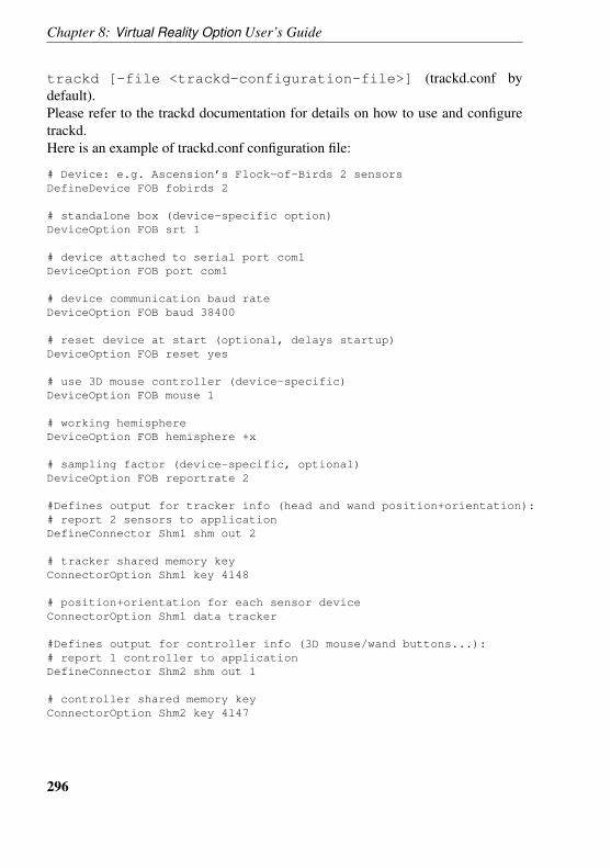
Chapter 8: Virtual Reality Option User’s Guide
trackd [-file <trackd-configuration-file>] (trackd.conf bydefault).Please refer to the trackd documentation for details on how to use and configuretrackd.Here is an example of trackd.conf configuration file:
# Device: e.g. Ascension’s Flock-of-Birds 2 sensorsDefineDevice FOB fobirds 2
# standalone box (device-specific option)DeviceOption FOB srt 1
# device attached to serial port com1DeviceOption FOB port com1
# device communication baud rateDeviceOption FOB baud 38400
# reset device at start (optional, delays startup)DeviceOption FOB reset yes
# use 3D mouse controller (device-specific)DeviceOption FOB mouse 1
# working hemisphereDeviceOption FOB hemisphere +x
# sampling factor (device-specific, optional)DeviceOption FOB reportrate 2
#Defines output for tracker info (head and wand position+orientation):# report 2 sensors to applicationDefineConnector Shm1 shm out 2
# tracker shared memory keyConnectorOption Shm1 key 4148
# position+orientation for each sensor deviceConnectorOption Shm1 data tracker
#Defines output for controller info (3D mouse/wand buttons...):# report 1 controller to applicationDefineConnector Shm2 shm out 1
# controller shared memory keyConnectorOption Shm2 key 4147
296
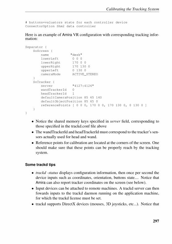
Calibrating the Tracking System
# buttons+valuators state for each controller deviceConnectorOption Shm2 data controller
Here is an example of Amira VR configuration with corresponding tracking infor-mation:
Separator {SoScreen {
name "desk"lowerLeft 0 0 0lowerRight 170 0 0upperRight 170 130 0upperLeft 0 130 0cameraMode ACTIVE_STEREO
}SoTracker {
server "4127:4126"wandTrackerId 0headTrackerId 1defaultCameraPosition 85 65 140defaultObjectPosition 85 65 0referencePoints [ 0 0 0, 170 0 0, 170 130 0, 0 130 0 ]
}}
• Notice the shared memory keys specified in server field, corresponding tothose specified in the trackd.conf file above
• The wandTrackerId and headTrackerId must correspond to the tracker’s sen-sors actually used for head and wand.
• Reference points for calibration are located at the corners of the screen. Oneshould make sure that these points can be properly reach by the trackingsystem.
Some trackd tips
• trackd -status displays configuration information, then once per second thedevice inputs such as coordinates, orientation, buttons state.... Notice thatAmira can also report tracker coordinates on the screen (see below).
• Input devices can be attached to remote machines. A trackd server can thenfowards inputs to the trackd daemon running on the application machine,for which the trackd license must be set.
• trackd supports DirectX devices (mouses, 3D joysticks, etc...). Notice that
297
Chapter 8: Virtual Reality Option User’s Guide
device name can be dependent on international language used on your com-puter.
• A controller device can be used to emulate a tracker.
8.6.3 Calibration step by step
Here is a complete step-by-step description of the calibration process.
1. Make sure that the trackd software is running and that the tracking systemis operating.
2. Start Amira and choose the appropriate configuration from the main win-dow’s VR menu.
3. In the AmiraVR control module, connect to the tracking system if necessary.Activate the values toggle in order to display the current 3D coordinates inthe upper left corner of the main screen. Make sure that the coordinates arechanging if you move the 3D input device and the head sensor (unless headtracking is disabled in the Virtual Reality Option config file). Also make surethat the button status changes if you press a button of the 3D input device.Note: Unless you are in calibration mode the coordinates reported by thevalues option are transformed coordinates, i.e., they are in the same coordi-nate system in which the screens in the config file have been defined.Hint: If the wand tracker and the head tracker seem to be exchanged modifythe fields wandTrackerId and headTrackerId in the Virtual Reality Optionconfig file.
4. Click the Calibrate button of the AmiraVR control module. You are now incalibration mode. A fixed 2D control grid is displayed on all screens. Youare requested to click at the first reference point (highlighted in red). In thecurrent version of Virtual Reality Option, the control grid is not guaranteed tomatch the actual reference points. However, you could choose the referencepoints in the config file to be at the corners of the control grid (one thirdand two thirds of the screen width in horizontal direction, one half of thescreen height in vertical direction). Besides the number of the referencepoint its coordinates as specified in the config file are displayed in the upperleft corner of the main screen.Now move the 3D input device at the first reference point and click anybutton of the device.
298
Calibrating the Tracking System
Note: Make sure that the raw tracker coordinates which are displayed in theupper left corner of the main screen are valid at the reference point. Somedevices just report zero values if the sensor is outside the operating range ofthe tracking system. Some other devices report non-sense values, typicallywith large oscillations. If you don’t get stable values at a reference point,choose some other point in the Virtual Reality Option config file.
5. Next you are asked to click at second reference point using the 3D inputdevice. Repeat the above procedure until all reference points have beenlocated.Note: If less than three different reference points are specified in the configfile, then by default the upper left, lower left, and lower right corners ofthe first screen are used as reference points. You may want to specify otherreference points or a larger number of reference points in order to improveaccuracy. The reference points must not lie all on one line. However, theymay well be located in a common plane, e.g., in the plane of the main screen.
6. Next, you need to align the glasses for head tracking. However, if headtracking is disabled in the Virtual Reality Option config file, this step is omit-ted.Align the glasses parallel to the x-axis of the screen coordinate system.Usually the x-axis will oriented horizontally with respect to the front screenof the display system. The up-direction of the glasses should be alignedparallel to the y-axis of the screen coordinate system. Usually the y-axiswill be oriented vertically with respect to the front screen. Once you havealigned the glasses click any button of the 3D input device.
7. Now camera calibration is done and correct stereoscopic images should bedisplayed. As a final step you are requested to pick the wand in order todefine the wand offset. The wand avatar is displayed half-way between thecurrent eye position (or the default camera position, if head tracking is dis-abled) and the default object position. Now move the 3D input device nearthe origin of the wand (or at any other position) and click any button. Thevirtual wand remains stuck to the 3D input device in exactly that position.You can repeat this last calibration step any time by clicking on the pickwand button of the AmiraVR module.
299
Chapter 8: Virtual Reality Option User’s Guide
Hint: If you don’t get a clear 3D image of the wand make sure left and righteye images are not exchanged. If the eyes are exchanged you get a resultwhich somehow also looks 3D but which isn’t comfortable to work with atall. Also make sure that the fields leftEyeOffset and rightEyeOffset are setcorrectly in the config file. You can optionally tune stereo eye offset withAmiraVR control module.
8. At this point, the calibration is finished. You may now want to write a newVirtual Reality Option config file (or to overwrite the original one) in orderto save the calibration data permanently. This can be achieved most easilyby pressing the write config button of the AmiraVR control module. Pressingthis button causes the Amira file browser to be activated. You can accept thename of the previous config file or choose a new one.When reloading the new configuration calibrated tracker data will be gener-ated automatically. You can verify the correctness of the calibration processby turning on the values toggle and moving the 3D input device to one ofthe reference points. The reported values should be almost the same as thecoordinates of the reference point specified in the config file.
Manual calibration
In some case you may want to enter directly in the configuration file the calibrationinformation corresponding to the defined reference points. The calibration fieldcontains the tracker coordinates for 3 points with following coordinates relative tothe screen’s reference defined by:origin x=0 y=0 z=0point1 x=X y=0 z=0, where X is the physical width of the first screen in config filepoint2 x=0 y=1 z=0For instance considering a screen of 170x130 cm, with tracker origin located inthe center/botton of the screen and tracker coordinates reported in meters, withsame axis x, y, z.- ReferencePoints: [0 0 0, 170 0 0, 170 130 0, 0 130 0]- Corresponding tracker coordinates: [0 0 0, 17 0 0, 17 13 0, 0 13 0]- Resulting calibration field: calibration [0 0 0, 17 0 0, 0 0.1 0]
300
3D User Interaction
Checking immersive displays
Here are some further hints for checking whether the immersive system is config-ured and working properly when used with stereo and head tracking:
• Does the virtual wand avatar follow the actual wand rotations ?With electromagnetic tracker, if rotations look wrong or reversed alongsome axis, the wand has probably crossed the tracker’s working hemispherewhen calibrating. Change the working hemisphere in trackd.conf and cali-brate again.
• Stereo disparity, reversed eyes ?If stereo effect looks too strong, uncomfortable or inconsistent, check screencoordinates in the configuration file and eye offset in configuration file orwith the AmiraVR module. For reversed eyes you may either change eyeoffsets, or change your system’s display properties, e.g. ’stereo reverse eyes’in display control panel.
• Is the plane of projection located on the physical screen ? The screen pro-jection of virtual objects located behind physical screen should look smalleras eyes get closer to the screen. Projection of virtual points located on thephysical screen shouldn’t move as eyes are moving. Otherwise check screencoordinates and tracker calibration.
• With multiple screens, do straight lines keep straight across screen edges ?Otherwise check screen coordinates, calibration, tracking, eye offset.
• Does wand avatar follow the sensor ? Otherwise check calibration andscreen coordinates.
8.7 3D User Interaction
Virtual Reality Option flat screen configurations, i.e., tiled displays or power walls,can be completely controlled using an ordinary 2D mouse. However, in case oftrue immersive configurations this isn’t feasible. Therefore, several ways of 3Duser interaction are provided in Virtual Reality Option. The view can be changedusing different navigation modes, a 3D menu is provided in order to control mod-ules in 3D, and special objects like slices, selection boxes, or 3D point probescan be directly picked and manipulated using a tracked input device. In addition,a 2D mouse mode is provided allowing the user to control the conventional 2Dmouse pointer using the tracked 3D mouse. In the following these features will be
301
Chapter 8: Virtual Reality Option User’s Guide
described in more detail.In order to utilize 3D user interaction a tracked 3D input device with at least onebutton is required. By default Amira only interprets a single button. The easiestway to make use of additional buttons is to associate Tcl procedures with thesebuttons. This is described below in a section about Tcl event procedures.
• The 3D menu• User-defined 3D menu items• 3D module controls• Navigation modes• Tcl event procedures• The 2D mouse mode
8.7.1 The 3D Menu
The Virtual Reality Option 3D menu provides buttons allowing the user to bring upa 3D version of the user interface of every object in the Pool. In addition it cancontain any number of user-defined buttons. These buttons can be configured mosteasily using the Tcl interface described in Section 8.7.2.By default, the menu also contains a button for activating the 2D mouse mode.This mode lets you control the 2D mouse using a 3D input device. In this way alsothe standard 2D user interface of Amira can be used in a VR environment.The basic shape of the Virtual Reality Option 3D menu is shown in Figure 8.6 onthe left hand side. The menu can be manipulated in the following way:
• Initially, after activating or reloading an Virtual Reality Option configura-tion, the 3D menu is hidden. In order to bring up the menu double-clickthe button of the 3D input device. Alternatively, you may select the 3Dmenu toggle button of the AmiraVR control module. By default the menuwill be positioned in the upper left corner of the first screen defined in theVirtual Reality Option config file. You may change the default position bysetting the field menuPosition in the tracker section of the Virtual RealityOptionconfig file. There is also a field for setting the default orientation ofthe menu.
• You can move the menu by pointing the wand on the blue header labeled3D menu, clicking the main button of the 3D input device, and then movingthe device while keeping the button pressed. When the wand is on the blueheader a yellow frame is displayed, indicating that this element has focus.
302
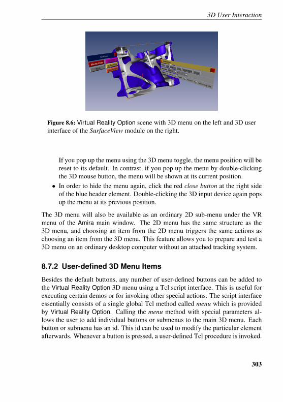
3D User Interaction
Figure 8.6: Virtual Reality Option scene with 3D menu on the left and 3D userinterface of the SurfaceView module on the right.
If you pop up the menu using the 3D menu toggle, the menu position will bereset to its default. In contrast, if you pop up the menu by double-clickingthe 3D mouse button, the menu will be shown at its current position.
• In order to hide the menu again, click the red close button at the right sideof the blue header element. Double-clicking the 3D input device again popsup the menu at its previous position.
The 3D menu will also be available as an ordinary 2D sub-menu under the VRmenu of the Amira main window. The 2D menu has the same structure as the3D menu, and choosing an item from the 2D menu triggers the same actions aschoosing an item from the 3D menu. This feature allows you to prepare and test a3D menu on an ordinary desktop computer without an attached tracking system.
8.7.2 User-defined 3D Menu Items
Besides the default buttons, any number of user-defined buttons can be added tothe Virtual Reality Option 3D menu using a Tcl script interface. This is useful forexecuting certain demos or for invoking other special actions. The script interfaceessentially consists of a single global Tcl method called menu which is providedby Virtual Reality Option. Calling the menu method with special parameters al-lows the user to add individual buttons or submenus to the main 3D menu. Eachbutton or submenu has an id. This id can be used to modify the particular elementafterwards. Whenever a button is pressed, a user-defined Tcl procedure is invoked.
303
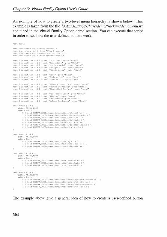
Chapter 8: Virtual Reality Option User’s Guide
An example of how to create a two-level menu hierarchy is shown below. Thisexample is taken from the file $AMIRA ROOT/share/demo/tracking/demomenu.hxcontained in the Virtual Reality Option demo section. You can execute that scriptin order to see how the user-defined buttons work.
menu reset
menu insertMenu -id 0 -text "Medical"menu insertMenu -id 1 -text "Flow Dynamics"menu insertMenu -id 2 -text "Reconstruction"menu insertMenu -id 3 -text "Multi-Channel"
menu 0 insertItem -id 0 -text "CT Slices" -proc "Menu0"menu 0 insertItem -id 1 -text "Isosurface" -proc "Menu0"menu 0 insertItem -id 2 -text "Surface model" -proc "Menu0"menu 0 insertItem -id 4 -text "Oblique slice" -proc "Menu0"menu 0 insertItem -id 5 -text "Pseudo-color" -proc "Menu0"
menu 1 insertItem -id 0 -text "Wing" -proc "Menu1"menu 1 insertItem -id 1 -text "Turbine ISL" -proc "Menu1"menu 1 insertItem -id 2 -text "Turbine LIC" -proc "Menu1"
menu 2 insertItem -id 0 -text "Slice & Isosurface" -proc "Menu2"menu 2 insertItem -id 1 -text "Volume Rendering" -proc "Menu2"menu 2 insertItem -id 2 -text "Simplified Surface" -proc "Menu2"
menu 3 insertItem -id 0 -text "Projection view" -proc "Menu3"menu 3 insertItem -id 1 -text "Slicing" -proc "Menu3"menu 3 insertItem -id 2 -text "Isosurface" -proc "Menu3"menu 3 insertItem -id 3 -text "Volume Rendering" -proc "Menu3"
proc Menu0 { id } {global AMIRA_ROOTswitch $id \
0 { load $AMIRA_ROOT/share/demo/medical/ctstack.hx } \1 { load $AMIRA_ROOT/share/demo/medical/isosurface.hx } \2 { load $AMIRA_ROOT/share/demo/medical/surf.hx } \3 { load $AMIRA_ROOT/share/demo/medical/tetra.hx } \4 { load $AMIRA_ROOT/share/demo/medical/gridcut.hx } \5 { load $AMIRA_ROOT/share/demo/medical/pseudocolor.hx } \6 { load $AMIRA_ROOT/share/demo/medical/splats.hx }
}
proc Menu1 { id } {global AMIRA_ROOTswitch $id \
0 { load $AMIRA_ROOT/share/demo/cfd/wing.hx } \1 { load $AMIRA_ROOT/share/demo/cfd/turbine-isl.hx } \2 { load $AMIRA_ROOT/share/demo/cfd/turbine-lic.hx }
}
proc Menu2 { id } {global AMIRA_ROOTswitch $id \
0 { load $AMIRA_ROOT/share/demo/recon/recon01.hx } \1 { load $AMIRA_ROOT/share/demo/recon/recon05.hx } \2 { load $AMIRA_ROOT/share/demo/recon/recon04.hx }
}
proc Menu3 { id } {global AMIRA_ROOTswitch $id \
0 { load $AMIRA_ROOT/share/demo/multichannel/projectionview.hx } \1 { load $AMIRA_ROOT/share/demo/multichannel/slicing.hx } \2 { load $AMIRA_ROOT/share/demo/multichannel/isosurfaces.hx }3 { load $AMIRA_ROOT/share/demo/multichannel/voltex.hx }
}
The example above give a general idea of how to create a user-defined button
304
3D User Interaction
hierarchy. The menu command provides some additional parameters. The generalform of the menu command is as follows:
menu [submenu-id [...]] cmd [options]
Here submenu-id is the id of any submenu. The root level has no id at all. Thefirst level has one id, the second level has two ids, and so on.
• a button for activating the 2D mouse mode (id 1000)• a button for getting a list of all modules (id 1001)• a button for getting a list of all data objects (id 1002)
You can remove these default buttons using the command menu clear. In orderto clear the menu and then reset the default buttons, use menu reset. Thecomplete list of commands is this:
menu resetRemoves all buttons and sub-menus from the menu and restores the defaultlayout with entries for mouse mode, modules, and data objects. This com-mand can only be applied at the main level.
menu [...] clearRemoves all buttons and sub-menus from the specified menu. If applied atthe main level also the default buttons (mouse mode, modules, and data) willbe removed.
menu [...] countReturns the number of entries (action buttons and sub-menu buttons) in thespecified menu.
menu [...] idAt index Returns the id of the item at position index.
menu [...] insertItem [options]This command creates a new button and inserts it into the specified menu.The following options are available:
-id idSpecifies the id of the new button.
-index indexSpecifies the position of the new button. If index is -1 (which is thedefault) the new button will be appended at the bottom of the menu.
305
Chapter 8: Virtual Reality Option User’s Guide
-text textSpecifies the text to be displayed by the new button.
-fg ”r g b”Specifies the text or foreground color of the new button.
-bg ”r g b”Specifies the background color of the new button.
-proc procThe name of the Tcl procedure to be called when the button is pressed.Either an own procedure without arguments can be used for a button.Alternatively, a procedure with one argument can be used for all but-tons in a menu. The argument then is set to the id of the pressed button(see example above).
menu [...] insertMenu [options]This command creates a new sub-menu button and inserts it into the speci-fied menu. The id of the new button can be used as a sub-menu id for themenu command itself. The same options as for insertItem can be used. Inaddition the following option is available:
-type classtypeIf this option is specified a special sub-menu will be inserted whichlists all objects of type classtype in the Amira Pool. For example, inorder to get a list of all modules (like in the default menu) you shoulduse insertMenu with -type HxModule.
menu [...] changeItem id -text textChanges the text of an existing button.
menu [...] removeItem idRemoves an action button or sub-menu button from the menu.
menu [...] connectItem id procConnects a button to a Tcl procedure. The procedure will be called whenthe button is pressed.
menu [...] disconnectItem id procDisconnects a button from a Tcl procedure.
306
3D User Interaction
8.7.3 3D Module Controls
The 3D menu provides a button called Modules. Clicking on this button brings upa list of all visible modules which currently exist in the Amira Pool. Clicking ona module button brings up a 3D version of the modules user interface. This 3Duser interface looks very similar to the 2D user interface of the module which isnormally shown in the Properties Area of the Amira main window. An example ofthe 3D user interface of the SurfaceView module is shown in Figure 8.6.The 3D user interface of every module can be moved independently from eachother like the main 3D menu itself. Again, this is done by picking the header barof the module’s GUI. The GUI can be removed by clicking on the red close buttonat the right side of the header bar. On the left side an orange viewer toggle isdisplayed. As in the 2D interface a display module can be switched on or off bytoggling this button.In 3D the ports of a module can be manipulated almost in the same way as in2D. The only remarkable difference is that text input is not possible in 3D. Textfields with numerical values like the range of a colormap port or the data windowof an OrthoSlice module still can be changed using a virtual slider. This is doneby clicking into the text field with the wand, and then moving the wand upwardsor downwards while keeping the button pressed. As a general rule, every activeelement shows a yellow frame when the wand is pointing on it, i.e., when it hasinput focus.
8.7.4 Navigation Modes
Virtual Reality Option supports two different navigation modes. The default modeis scene manipulation, i.e., the whole scene can be rotated and translated usingthe 3D input device. This is done by clicking with the wand into some empty orinsensitive region in space, and then moving the wand while keeping the buttonpressed. In this mode the whole scene remains stick relative to the input device.The second mode is fly mode. This mode can be activated by selecting the secondentry from the Mode port of the AmiraVR control module (either in the 2D or inthe 3D user interface). In fly mode you can click the 3D input device at someinsensitive point, and then move it in any direction. The vector from the pointwhere the wand was clicked to the current point defines a velocity vector which isused to modify the position of the camera. The longer the vector, i.e., the more thewand is shifted, the faster the camera is moving. In the same way the orientation ofthe camera is modified by rotating the 3D wand. An incremental rotational change
307
Chapter 8: Virtual Reality Option User’s Guide
is computed by comparing the current orientation which the orientation at the pointwhere the wand was clicked initially.
8.7.5 Tcl Event Procedures
By default, Virtual Reality Option treats all buttons of a 3D mouse in the same way.This allows you to operate the program even with a one-button mouse. In order tomake better use of a 3D input device with multiple buttons, you can define specialTcl procedures which are called when a button is pressed or released. If theseprocedures return the value 1, this indicates that the event has been handled by theTcl procedure and that it should not be further processed by Amira. In particular, itthen will not be send to the Open Inventor scene graph. The following procedurescan be defined:
• vrButton0Press, vrButton1Press, ...These procedures are called when the button with the specified index ispressed. By redefining vrButton0Press you can overwrite the defaultinteraction routine.
• vrButton0Release, vrButton1Release, ...These procedures are called when the button with the specified index is re-leased.
• vrButton0DblClick, vrButton1DblClick, ...These procedures are called when the button with the specified index isdouble-clicked. Note that for the first click of a double-click event an or-dinary button press event is generated.
When a 3D mouse button event occurs and no appropriate Tcl event procedure isdefined or if this procedure returns 0, the event will be passed to the current VirtualReality Option event handler. The default event handler checks if the 3D menuor some other 3D widget has been clicked. If not, it sends the event to the OpenInventor scene graph. Besides this default event handler there are also other eventhandlers, namely handlers for managing the different navigation modes (examineand fly).If a 3D mouse button event was not handled by the current event handler, finallythe following Tcl procedures will be called, provided they are defined:
vrButton0PressFallback, vrButton1PressFallback, ...vrButton0ReleaseFallback, vrButton1ReleaseFallback, ...vrButton0DblClickFallback, vrButton1DblClickFallback, ...
308
3D User Interaction
Assuming that the default event handler is active (the one which checks the 3Dmenu and the Open Inventor scene graph), you can trigger certain actions when theuser clicks into empty space. By default, when this happens one of the navigationmode handlers is activated. If you want to disable this feature you can define adummy vrButton0PressFallback procedure which always returns 1.
8.7.6 The 2D Mouse mode
The 2D mouse mode is useful for accessing GUI elements which have no directanalogy in 3D. In this mode the position of the ordinary 2D mouse pointer iscontrolled using the 3D input device.
• In order to activate 2D mouse mode press the red mouse mode button of the3D menu. Once mouse mode is activated the Amira main window is poppedup automatically.
• You can control the 2D mouse by translating or rotating the 3D input device.Usually, rotating it is more convenient since less movement is required. Theposition of the 2D mouse is computed by determining the intersection of thevirtual wand vector with the screen.
• In order to exit 2D mouse mode, double-click the 3D input device over someinsensitive region of the 2D user interface. When leaving 2D mouse modethe main graphics window is raised automatically.If the 2D mouse stays in the middle of the screen, of course 3D impressionis disturbed. Therefore, usually it is a good idea to move the 2D mouse in acorner before returning to 3D mode.
The two Tcl procedures VRSettings StartMouseMode and VRSet-tings StopMouseMode are called when entering and exiting 2D mousemode. You can use these methods for example to pop up the Amira helpbrowser with a page from which additional demos can be launched. Forthis, the following definition could be included for example in the file$AMIRA ROOT/share/resources/Amira/Amira.init:
proc VRSettings\_StartMouseMode { } {global AMIRA ROOTload $AMIRA ROOT/share/usersguide/tracking.html
}In order to activate or deactivate the 2D mouse mode from Tcl, the Vir-tual Reality Option control module provides the command VRSettings
309
Chapter 8: Virtual Reality Option User’s Guide
enableMouseMode <value>, where <value> can be either 0 or 1. In or-der to check if 2D mouse mode is currently active, you can use VRSettingsisMouseModeEnabled.
8.8 Writing Virtual Reality Option Custom Modules
Amira can be easily extended by writing new I/O routines, data types, modules,and other components. Details about this are described in the Developer OptionUser’s Guide.In order to write custom modules which provide specific interaction features ina VR environment, Open Inventor nodes interpreting events generated by the 3Dinput device have to be inserted into the scene graph. In particular, the 3D in-put device generates events of type SoTrackerEvent and SoControllerButtonEvent.These two event classes have been introduced in Open Inventor 3.0. For moreinformation about these classes please refer to the Open Inventor documentation.Amira itself provides an additional class Hx3DWandBase which provides someadditional information about the virtual 3D wand. Among others, this class alsoallows to user to highlight the wand in order to provide some visual feedback dur-ing interaction.Below we present the source code of a sample AmiraVR module which just dis-plays a number of cubes. The cubes then can be picked and transformed using the3D wand. The source code of the module is contained in the Developer Optiondemo package. The particular files are called MyVRDemo.h and MyVRDemo.cpp.The module can also be directly created from the popup menu of the AmiraVRcontrol module.Here is the listing of the header file:
///////////////////////////////////////////////////////////////////////// Illustrates 3D interaction in a VR environment///////////////////////////////////////////////////////////////////////#ifndef MY_VR_DEMO_H#define MY_VR_DEMO_H
#include <Inventor/nodes/SoSeparator.h>
#include <McHandle.h>#include <Amira/HxModule.h>#include <Amira/HxPortButtonList.h>#include <mypackage/mypackageAPI.h>
class MYPACKAGE_API MyVRDemo : public HxModule
310
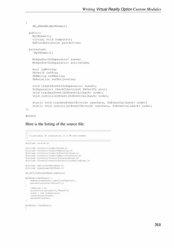
Writing Virtual Reality Option Custom Modules
{HX_HEADER(MyVRDemo);
public:MyVRDemo();virtual void compute();HxPortButtonList portAction;
protected:˜MyVRDemo();
McHandle<SoSeparator> scene;McHandle<SoSeparator> activeCube;
bool isMoving;SbVec3f refPos;SbMatrix refMatrix;SbRotation refRotInverse;
void createScene(SoSeparator* scene);SoSeparator* checkCube(const SbVec3f& pos);void trackerEvent(SoEventCallback* node);void controllerEvent(SoEventCallback* node);
static void trackerEventCB(void* userData, SoEventCallback* node);static void controllerEventCB(void* userData, SoEventCallback* node);
};
#endif
Here is the listing of the source file:///////////////////////////////////////////////////////////////////////// Illustrates 3D interaction in a VR environment///////////////////////////////////////////////////////////////////////#include <stdlib.h>
#include <Inventor/nodes/SoCube.h>#include <Inventor/nodes/SoMaterial.h>#include <Inventor/nodes/SoEventCallback.h>#include <Inventor/nodes/SoMatrixTransform.h>#include <Inventor/events/SoTrackerEvent.h>#include <Inventor/events/SoControllerButtonEvent.h>
#include <Amira/Hx3DWandBase.h>#include <mypackage/MyVRDemo.h>
HX_INIT_CLASS(MyVRDemo,HxModule)
MyVRDemo::MyVRDemo() :HxModule(HxObject::getClassTypeId()),portAction(this,"action",1)
{isMoving = 0;portAction.setLabel(0,"Reset");scene = new SoSeparator;createScene(scene);showGeom(scene);
}
MyVRDemo::˜MyVRDemo(){
311
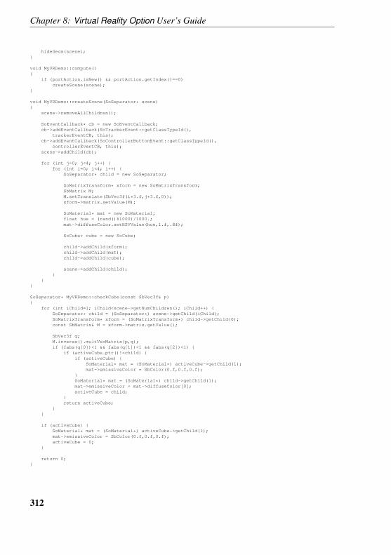
Chapter 8: Virtual Reality Option User’s Guide
hideGeom(scene);}
void MyVRDemo::compute(){
if (portAction.isNew() && portAction.getIndex()==0)createScene(scene);
}
void MyVRDemo::createScene(SoSeparator* scene){
scene->removeAllChildren();
SoEventCallback* cb = new SoEventCallback;cb->addEventCallback(SoTrackerEvent::getClassTypeId(),
trackerEventCB, this);cb->addEventCallback(SoControllerButtonEvent::getClassTypeId(),
controllerEventCB, this);scene->addChild(cb);
for (int j=0; j<4; j++) {for (int i=0; i<4; i++) {
SoSeparator* child = new SoSeparator;
SoMatrixTransform* xform = new SoMatrixTransform;SbMatrix M;M.setTranslate(SbVec3f(i*3.f,j*3.f,0));xform->matrix.setValue(M);
SoMaterial* mat = new SoMaterial;float hue = (rand()%1000)/1000.;mat->diffuseColor.setHSVValue(hue,1.f,.8f);
SoCube* cube = new SoCube;
child->addChild(xform);child->addChild(mat);child->addChild(cube);
scene->addChild(child);}
}}
SoSeparator* MyVRDemo::checkCube(const SbVec3f& p){
for (int iChild=1; iChild<scene->getNumChildren(); iChild++) {SoSeparator* child = (SoSeparator*) scene->getChild(iChild);SoMatrixTransform* xform = (SoMatrixTransform*) child->getChild(0);const SbMatrix& M = xform->matrix.getValue();
SbVec3f q;M.inverse().multVecMatrix(p,q);if (fabs(q[0])<1 && fabs(q[1])<1 && fabs(q[2])<1) {
if (activeCube.ptr()!=child) {if (activeCube) {
SoMaterial* mat = (SoMaterial*) activeCube->getChild(1);mat->emissiveColor = SbColor(0.f,0.f,0.f);
}SoMaterial* mat = (SoMaterial*) child->getChild(1);mat->emissiveColor = mat->diffuseColor[0];activeCube = child;
}return activeCube;
}}
if (activeCube) {SoMaterial* mat = (SoMaterial*) activeCube->getChild(1);mat->emissiveColor = SbColor(0.f,0.f,0.f);activeCube = 0;
}
return 0;}
312
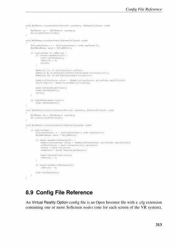
Config File Reference
void MyVRDemo::trackerEventCB(void* userData, SoEventCallback* node){
MyVRDemo* me = (MyVRDemo*) userData;me->trackerEvent(node);
}
void MyVRDemo::trackerEvent(SoEventCallback* node){
SoTrackerEvent* e = (SoTrackerEvent*) node->getEvent();Hx3DWandBase* wand = GET_WAND(e);
if (activeCube && isMoving) {if (!wand->getButton(0)) {
node->setHandled();isMoving = 0;return;
}
SbMatrix T1; T1.setTranslate(-refPos);SbMatrix R; R.setRotate(refRotInverse*wand->orientation());SbMatrix T2; T2.setTranslate(wand->origin());
SoMatrixTransform* xform = (SoMatrixTransform*) activeCube->getChild(0);xform->matrix = SbMatrix(refMatrix*T1*R*T2);
wand->setHighlight(true);node->setHandled();return;
}
if (checkCube(wand->top()))node->setHandled();
}
void MyVRDemo::controllerEventCB(void* userData, SoEventCallback* node){
MyVRDemo* me = (MyVRDemo*) userData;me->controllerEvent(node);
}
void MyVRDemo::controllerEvent(SoEventCallback* node){
if (activeCube) {SoTrackerEvent* e = (SoTrackerEvent*) node->getEvent();Hx3DWandBase* wand = GET_WAND(e);
if (wand->wasButtonPressed(0)) {SoMatrixTransform* xform = (SoMatrixTransform*) activeCube->getChild(0);refRotInverse = wand->orientation().inverse();refPos = wand->origin();refMatrix = xform->matrix.getValue();
wand->setHighlight(true);isMoving = 1;
}
if (wand->wasButtonReleased(0))isMoving = 0;
node->setHandled();}
}
8.9 Config File Reference
An Virtual Reality Option config file is an Open Inventor file with a .cfg extensioncontaining one or more SoScreen nodes (one for each screen of the VR system),
313
Chapter 8: Virtual Reality Option User’s Guide
optional nodes SoTracker (containing information about the tracking system) andSoVRProperty (containing general information), as well as optional Open Inventornodes (containing possibly a visual representation of the room).In principle two different configurations are distinguished. A ”flat screen” con-figuration defines a virtual big 2D screen, while a true ”immersive” configurationdefines multiple screens in a non-planar configuration. For a flat screen configura-tion, the fields tileOrigin and tileSize (see below) are used, while for an immersiveconfiguration the fields lowerLeft, lowerRight, upperRight, and upperLeft are used.For a tiled configuration, ordinary 2D mouse interaction works, while an immer-sive configuration usually requires a tracking system.By default, the list of available config files (*.cfg) is generated by looking inthe AMIRA ROOT/share/config/vr and AMIRA LOCAL/share/config/vr directories.The user can define an AMIRA VR CONFIGS PATH environment variable to usea different location at start-up. Then, at runtime, the list can be further changed orupdated by using the Change Configs Path... item in the VR menu.
SoScreen
An SoScreen node can contain the fields detailed below. The field content typeis given inside brackets using Open Inventor conventions, ie. SoSFVec3f standsfor ’a vector of 3 float values’, SoSFRotation is a rotation defined with 4 valuesrepresents an axis of rotation followed by the amount of right-handled rotationabout that axis, in radians. For example, a 180 degree rotation about the Y axis is: 0 1 0 3.12159265
SoSFString name ”Vertical screen”The name of the screen (not used internally)
SoSFVec3f lowerLeft 0 0 0The coordinates of the lower left corner of the screen. Any right-handed co-ordinate system can be used. It does not matter in which units the screen cor-ners are defined because the transformation between the screen coordinatesand the tracker coordinates is computed automatically when calibrating thetracking system.
SoSFVec3f lowerRight 180 0 0The coordinates of the lower right corner of the screen.
314
Config File Reference
SoSFVec3f upperRight 180 110 0The coordinates of the upper right corner of the screen.
SoSFVec3f upperLeft 0 110 0The coordinates of the upper left corner of the screen.
SoSFString display ”:0.1”Specifies on which X display the screen should be rendered. On a multi-pipemachine such as an SGI Onyx, either different X servers may run on the dif-ferent pipes, or there may be one X server with multiple screens. Dependingon the actual configuration either ”:1.0” or ”:0.1” should be specified in or-der to enable multi-pipe rendering for the second screen. If this field isomitted, the window will be opened on the same display as the Amira userinterface (determined by the value of the DISPLAY environment variable orby the -display command line option).
SoSFString hostnameThis field is required if Virtual Reality Option will be run in cluster mode. Itspecifies on which node of a graphics cluster the particular screen should berendered. The hostname can either be specified as a name or as a numericIP address. See section 8.3 (Using Virtual Reality Option on a cluster).
SoSFVec2f channelOrigin 0.0 0.0Specifies the position of the upper left corner of the graphics window inrelative coordinates. (0,0) is the upper left corner of the desktop, (1,1) is thelower right corner of the desktop.
SoSFVec2f channelSize 0.5 1.0Specifies the size of graphics window in relative coordinates. The size ofthe whole desktop is (1,1). In order to create a window covering the lefthalf of the desktop, channelOrigin should be (0,0) and channelSize shouldbe (0.5,1).
SoSFVec2f tileOrigin 0.0 0.0This field is used in the case of a 2D tiled display instead of the fields lower-Left, lowerRight, upperRight, and upperLeft. It specifies the origin of a rect-angular part of a virtual big screen which should be rendered in the graphicswindow. The origin can be any point between (0,0) and (1,1). Here (0,0)denotes the LOWER left corner of the virtual big screen, and (1,1) denotesthe UPPER right corner.
315
Chapter 8: Virtual Reality Option User’s Guide
SoSFVec2f tileSize 1.0 1.0This field is used in the case of a 2D tiled display instead of the fields lower-Left, lowerRight, upperRight, and upperLeft. It specifies the size of a rectan-gular part of a virtual big screen which should be displayed in the graphicswindow. The size can be any value between (0,0) and (1,1).
SoSFEnum cameraMode [ MONOSCOPIC — LEFT VIEW — RIGHT VIEW— ACTIVE STEREO ]This field specifies the camera mode used for the screen. The default isMONOSCOPIC. The values LEFT VIEW and RIGHT VIEW are used forpassive stereo applications. If ACTIVE STEREO is specified, the windowis opened in active stereo mode by default.
SoSFEnum backgroundMode [ BG AS IS — BG LOWER — BG UPPER —BG REVERSE ]This field affects how the default Amira gradient background is renderedon the screen. If BG LOWER or BG UPPER is specified, a uniform back-ground with either the lower or upper color of the standard gradient back-ground is used. This is useful for the floor or ceiling of a CAVE.
SoSFInt32 threadGroupScreens with different thread groups are rendered in parallel using multiplethreads, provided Amira has been started with the -mt command line op-tion or the environment variable AMIRA MULTITHREAD has been set. Ifthe same thread group is used for two different screens, these screens willalways be rendered one after the other. Note that for all common currentgraphics architectures it makes no sense to render multiple windows on thesame pipe in parallel. Typically, this even implies a significant performancedecrease. Usually, screens being rendered on the same pipe (same displaybut different channelOrigin or channelSize) should be assigned the samethread group. Thread group and -mt command line option are only relevanton multipipe systems and do not apply to cluster systems.
SoMFFloat softEdgeOverlapThis field is used for soft-edge blending. It should contain exactly fourfloating-point values, indicating the size of the soft-edge region on the left,right, bottom, and top border of the screen relative to the total width or heightof the screen. For example, in order to specify a 25% soft-edge at the rightborder, softEdgeOverlap should be [ 0.0, 0.25, 0.0, 0.0 ].
316
Config File Reference
SoMFFloat softEdgeGammaThis field is used for soft-edge gamma correction. It should contain exactlyfour floating-point values, indicating the gamma value of the soft-edge re-gion at the left, right, bottom, and top border of the screen. A gamma valueof 1 means, that image intensity is linearly faded out to black. For mostprojectors, gamma values bigger than 1 are required to achieve good results.The default gamma value for all borders is 1.2.
SoTracker
An SoTracker node contains information about the tracking system. Usually itis not necessary to define an SoTracker node for a ”tiled” configuration, but onlyfor true VR configurations which make use of the fields lowerLeft, lowerRight,upperRight, and upperLeft of SoScreen (see above).
SoSFString server 4127:4126This field specifies a string used to initialize the connection to the track-ing system. In order to connect to a running VRCO trackd daemon, thestring should contain the shared memory key of the trackd controller data,and the shared memory key of the trackd tracker data separated by a colon(”¡controllerKey¿:¡trackerKey¿”). The shared memory keys are defined inthe trackd.conf file.
SoSFBool autoConnectIf this field is set to TRUE, the connection to the tracking system will be es-tablished automatically when the configuration is loaded. The default valueis FALSE.
SoSFVec3f defaultCameraPosition 90 50 150Defines the camera position to be used as long as there is no connection tothe tracking system. This position is also used if the head tracker id (below)is -1.
SoSFVec3f defaultObjectPosition 90 50 0Defines the object position to be used as long as there is no connection to thetracking system. If there is a ”view all” request in Amira (e.g., because thespace bar of the keyboard was hit), the scene is centered at the default objectposition. In a CAVE it makes sense to choose the default object position inthe center of the front wall.
317
Chapter 8: Virtual Reality Option User’s Guide
SoMFVec3f calibrationThe field is used to store calibration data, i.e., data allowing the system totransform raw tracker data into the coordinate system in which the screenshave been defined. Usually there is no need to set this field manually. In-stead, load a configuration file without calibration data, perform calibrationin Virtual Reality Option, and then export a new config file.
SoSFRotation rotGlassesThis field is used for calibrating the orientation of the tracked stereo glasses.Usually there is no need to set this field manually.
SoSFRotation rotWandThis field is used for calibrating the orientation of the wand tracker. Usuallythere is no need to set this field manually.
SoSFVec3f leftEyeOffsetThe center of the left eye with respect to the head tracker. For calibration,the glasses must be align parallel to the front screen. In this position the hor-izontal axis is the x-axis, the vertical axis is the y-axis, and the axis pointingtowards the observer is the z-axis. The eye offsets are defined with respectto this coordinate system. The difference between the left eye’s x-offset andthe right eye’s x-offset should be around 6.5 cm (average eye separation).
SoSFVec3f rightEyeOffsetThe center of the right eye with respect to the head tracker. The same re-marks as for leftEyeOffset apply.
SoMFVec3f referencePointsReference points used for calibrating the tracking system. If no referencepoints are specified, the user is asked to click at the upper left, lower left,and lower right corner of the first screen defined in the config file. Note thatat least three different reference points are required and that these pointsmust not lie on a common line. However, the reference points may well liein a common plane, e.g., in the screen plane itself.
SoSFInt32 wandTrackerIdSpecifies the id of the trackd sensor which should be used to control thewand. By default the wand sensor is assumed to have the id 0.
SoSFInt32 headTrackerIdSpecifies the id of the trackd sensor which should be used to control the
318
Config File Reference
camera (head tracking). By default the head tracker is assumed to have theid 1. If -1 is specified for a head tracker id, the default camera position isused instead of actually querying a head sensor.
SoSFInt32 headTrackingEnabledThis field determines if head tracking should be enabled or disabled by de-fault if the configuration file is loaded. The default is TRUE. If the value isset to FALSE, head tracking is initially disabled, but can be activated later bypressing the head tracking toggle of the AmiraVR control module. However,headTrackerId must not be set to -1 in this case.
SoSFString wandFileThis is the name of an Open Inventor file which is used as the visual rep-resentation of the wand. The origin of the wand should be at (0,0,0). Thewand itself should point into the negative z direction. The wand is scaled sothat the length 1 corresponds to 0.16 times the width of the first screen in theconfig file. The hot spot of the wand should be indicated by an SoInfo nodecontaining a string ”x y z”. Usually the hot spot will be something like ”00 -1”. The filename can be an absolute or relative path. If it is relative, thefile is assumed to be in the same directory as the config file itself (namely inshare/config/vr).
SoSFString highlightWandFileThis is the name of an Open Inventor file which is used as the visual repre-sentation of the wand in highlight state. The same remarks as for wandFileapply to this field too.
SoSFFloat wandScaleThis field specifies a scaling factor applied to the wand geometry. By de-fault, a value of 0.16 times the width of the first screen is assumed. In orderto change the length of the wand you can either specify a custom wand filewith a hot spot different from ”0 0 -1”, or you can change the wand scalevalue.
SoSFVec3f menuPositionSpecifies the default position of the upper left corner of the 3D menu. Bydefault it is placed in the upper left corner of the first screen in the config file.The values must be defined in the same coordinate system as the corners ofthe screens.
319
Chapter 8: Virtual Reality Option User’s Guide
SoSFRotation menuOrientationSpecifies the orientation of the 3D menu. By default the horizontal axis ofthe menu, i.e., the text direction, is aligned to the x-axis of the VR coordi-nate system, while the vertical direction is aligned to the y-axis. This fieldallows you to change the orientation by applying a rotation to the defaultorientation. The rotation is specified by four numbers. The first three num-bers define the axis of rotation, and the fourth numbers defines the rotationangle in radians.
SoSFFloat menuSizeThis field specifies the default width of the 3D menu in the same coordinatesin which the corners of the screens were defined. You can adjust this valueto make the menu smaller or bigger.
SoSFString onLoadThis field defines a Tcl command which is executed after the configura-tion has been loaded. You can put additional initialization code here. Forexample, you may always want to load a particular script MenuInit.hx forinitializing the 3D menu when a certain configuration is loaded. You can dothis by defining onLoad ”load $AMIRA ROOT/MenuInit.hx”.As another example you can show 3D menu with:onLoad ”AmiraVR options setValue 2 1”
SoSFString onUnloadThis field defines a Tcl command which is executed before a configurationis unloaded.
SoSFString onConnectThis field defines a Tcl command which is executed after a connection to thetracking system has been established.
SoSFString onDisconnectThis field defines a Tcl command which is executed after the connection tothe tracking system has been disconnected.
SoVRProperty
An SoVRProperty node contains general information about the Amira user inter-face.
320
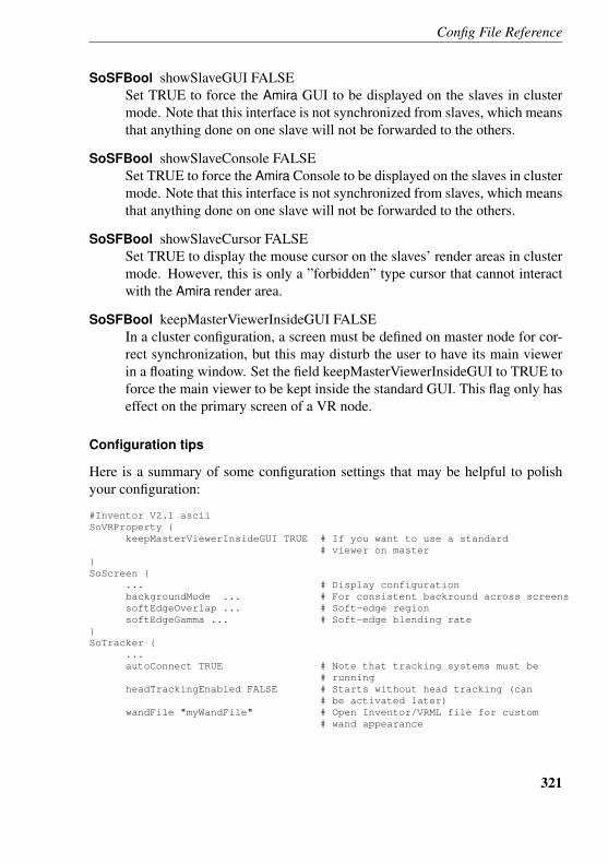
Config File Reference
SoSFBool showSlaveGUI FALSESet TRUE to force the Amira GUI to be displayed on the slaves in clustermode. Note that this interface is not synchronized from slaves, which meansthat anything done on one slave will not be forwarded to the others.
SoSFBool showSlaveConsole FALSESet TRUE to force the Amira Console to be displayed on the slaves in clustermode. Note that this interface is not synchronized from slaves, which meansthat anything done on one slave will not be forwarded to the others.
SoSFBool showSlaveCursor FALSESet TRUE to display the mouse cursor on the slaves’ render areas in clustermode. However, this is only a ”forbidden” type cursor that cannot interactwith the Amira render area.
SoSFBool keepMasterViewerInsideGUI FALSEIn a cluster configuration, a screen must be defined on master node for cor-rect synchronization, but this may disturb the user to have its main viewerin a floating window. Set the field keepMasterViewerInsideGUI to TRUE toforce the main viewer to be kept inside the standard GUI. This flag only haseffect on the primary screen of a VR node.
Configuration tips
Here is a summary of some configuration settings that may be helpful to polishyour configuration:
#Inventor V2.1 asciiSoVRProperty {
keepMasterViewerInsideGUI TRUE # If you want to use a standard# viewer on master
}SoScreen {
... # Display configurationbackgroundMode ... # For consistent backround across screenssoftEdgeOverlap ... # Soft-edge regionsoftEdgeGamma ... # Soft-edge blending rate
}SoTracker {
...autoConnect TRUE # Note that tracking systems must be
# runningheadTrackingEnabled FALSE # Starts without head tracking (can
# be activated later)wandFile "myWandFile" # Open Inventor/VRML file for custom
# wand appearance
321
Chapter 8: Virtual Reality Option User’s Guide
highlightWandFile "myHWandFile" # Highlighted versionmenuPosition 100 100 0 #menuSize 50 #onLoad "..." # Custom TCL commandsonConnect "..."onDisconnect "..."
}Separator { # Separator containing "environment
# scene"PointLight {location 0 0 0} # Useful e.g. in CAVEsSeparator {...} # Fixed geometry relative to screens
}
8.9.1 Tracker Emulator
The Tracker Emulator provides emulation of a 3D positioning device with twospatial sensors and two buttons. To activate it, type the word test into the trackerport of the AmiraVR control module and press the connect button. After that theuser interface dialog of the tracker emulator appears.As mentioned before, the emulator emulates two spatial sensors designated as sen-sor0 and sensor1. For each of these sensors the position is changeable by threesliders, one for each direction. Alternatively, as well as to reach positions of greaterdistance than the sliders allow, one can type the values directly into the text entryfields to the right of the slider.The sensor’s rotation can be changed by selecting one of the main axes as therotation axis and then further adjusting the rotation angle around this axis using theslider or the entry field. To perform an additional rotation, simply select a differentrotation axis and angle. The rotations are performed cumulatively. The currentrotation doesn’t affect the orientation of the main rotation axes. The rotation centeris always the current sensor position. To set the sensor’s rotation to the initialunrotated state, press the Reset button.In the buttons section one can toggle the emulated button’s state. As long as thecheckbox is checked, the emulated button is ”down”. If it’s unchecked, the emu-lated button is ”up”.
322
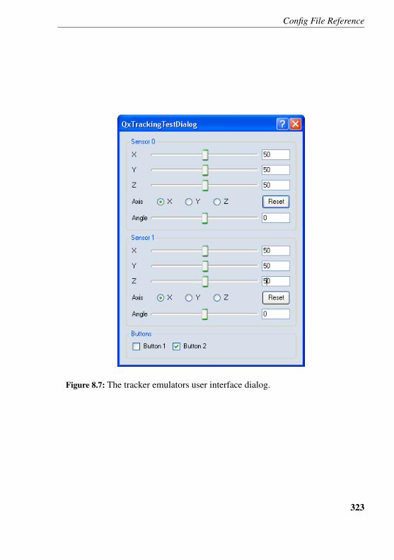
Config File Reference
Figure 8.7: The tracker emulators user interface dialog.
323

Part IV
Very Large Data OptionUser’s Guide
325

9 Very Large Data Option User’sGuide
9.1 Working with out-of-core data files (LDA)
The out-of-core management tools allow you load and visualize data sets largerthan the amount of RAM installed on your system, as well as convert these datasets into LDA (Large Data Access) files. These LDA files can be used to visual-ize very large data (hundreds of gigabytes), such as seismic or microscopy data,using a limited amount of memory. It is possible to convert original data of thefollowing types: AmiraMesh, RawData, and StackedSlices (stacks of SGI, TIFF,GIF, JPEG, BMP, PNG, JPEG2000, PGX, PNM, and RAS raster files). LDA dataallows subvolume extraction to display parts of the volume, or multi-resolutionaccess to have a full subsampled view or accurate refined local views.In particular, the following topics will be discussed in this tutorial:
1. Adjusting the size threshold to allow conversion2. Loading the out-of-core data3. Raw data parameters4. Out-of-core conversion5. Displaying an ortho slice, an oblique slice, and a 3D volume
Please follow the instructions below. Each step builds on the step before.
9.1.1 Tune the Size Threshold to Allow Conversion
In the Edit menu, select the Preferences item. This opens the AmiraPreferencesdialog. Please select the LDA tab (see Figure 9.1). Using the slider or text field, setthe threshold to 32MB. When you load a file of file size greater than this threshold,the out-of-core data dialog will be displayed.Note: To see the images as laid out in this tutorial, you should also use the Layouttab of the Edit/Preferences menu, and toggle on show viewer in top-level window.
327
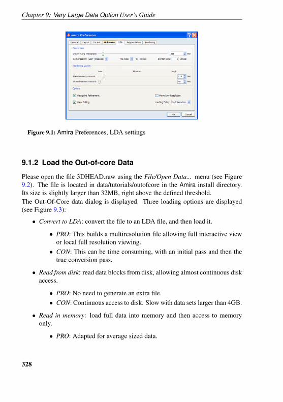
Chapter 9: Very Large Data Option User’s Guide
Figure 9.1: Amira Preferences, LDA settings
9.1.2 Load the Out-of-core Data
Please open the file 3DHEAD.raw using the File/Open Data... menu (see Figure9.2). The file is located in data/tutorials/outofcore in the Amira install directory.Its size is slightly larger than 32MB, right above the defined threshold.The Out-Of-Core data dialog is displayed. Three loading options are displayed(see Figure 9.3):
• Convert to LDA: convert the file to an LDA file, and then load it.
• PRO: This builds a multiresolution file allowing full interactive viewor local full resolution viewing.
• CON: This can be time consuming, with an initial pass and then thetrue conversion pass.
• Read from disk: read data blocks from disk, allowing almost continuous diskaccess.
• PRO: No need to generate an extra file.• CON: Continuous access to disk. Slow with data sets larger than 4GB.
• Read in memory: load full data into memory and then access to memoryonly.
• PRO: Adapted for average sized data.
328
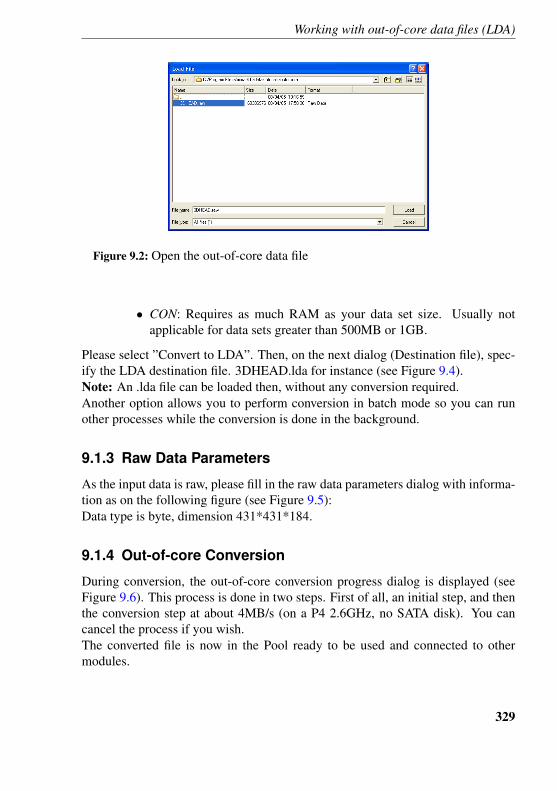
Working with out-of-core data files (LDA)
Figure 9.2: Open the out-of-core data file
• CON: Requires as much RAM as your data set size. Usually notapplicable for data sets greater than 500MB or 1GB.
Please select ”Convert to LDA”. Then, on the next dialog (Destination file), spec-ify the LDA destination file. 3DHEAD.lda for instance (see Figure 9.4).Note: An .lda file can be loaded then, without any conversion required.Another option allows you to perform conversion in batch mode so you can runother processes while the conversion is done in the background.
9.1.3 Raw Data Parameters
As the input data is raw, please fill in the raw data parameters dialog with informa-tion as on the following figure (see Figure 9.5):Data type is byte, dimension 431*431*184.
9.1.4 Out-of-core Conversion
During conversion, the out-of-core conversion progress dialog is displayed (seeFigure 9.6). This process is done in two steps. First of all, an initial step, and thenthe conversion step at about 4MB/s (on a P4 2.6GHz, no SATA disk). You cancancel the process if you wish.The converted file is now in the Pool ready to be used and connected to othermodules.
329
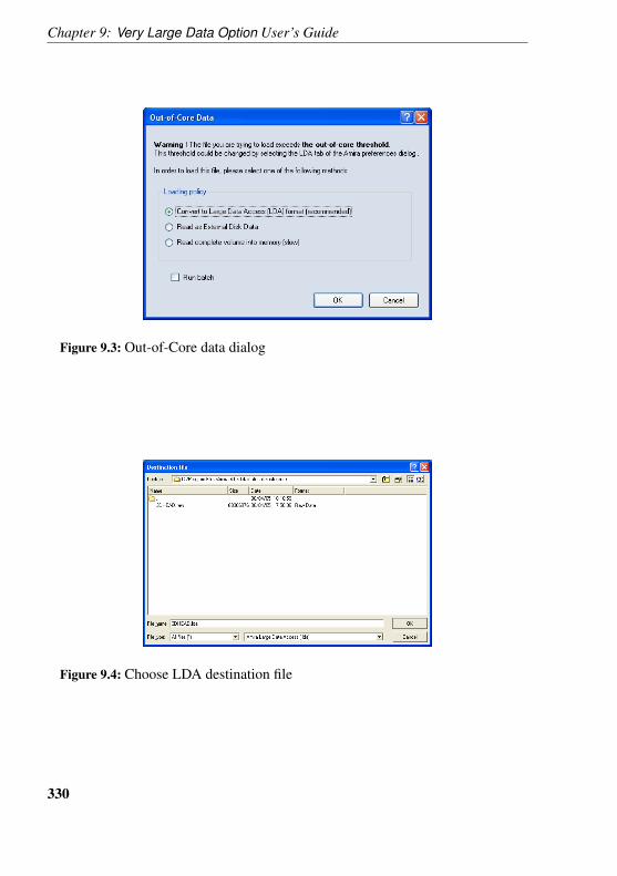
Chapter 9: Very Large Data Option User’s Guide
Figure 9.3: Out-of-Core data dialog
Figure 9.4: Choose LDA destination file
330
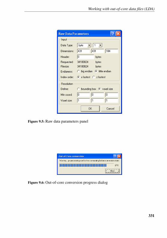
Working with out-of-core data files (LDA)
Figure 9.5: Raw data parameters panel
Figure 9.6: Out-of-core conversion progress dialog
331
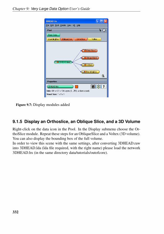
Chapter 9: Very Large Data Option User’s Guide
Figure 9.7: Display modules added
9.1.5 Display an Orthoslice, an Oblique Slice, and a 3D Volume
Right-click on the data icon in the Pool. In the Display submenu choose the Or-thoSlice module. Repeat these steps for an ObliqueSlice and a Voltex (3D volume).You can also display the bounding box of the full volume.In order to view this scene with the same settings, after converting 3DHEAD.rawinto 3DHEAD.lda (lda file required, with the right name) please load the network3DHEAD.hx (in the same directory data/tutorials/outofcore).
332
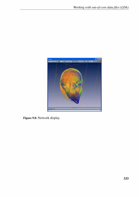
Working with out-of-core data files (LDA)
Figure 9.8: Network display
333


Part V
Quantification+ Option User’sGuide
335

Working with out-of-core data files (LDA)
This extension integrates the Visilog product by Noesis into Amira. The Quantifi-cation+ Option, with its wide range of image processing tools, can be used togetherwith the 3D visualization and geometry reconstruction capabilities of Amira.A set of demos is provided. For details, see the documentation of the Visilogmodule.
337

Part VI
Microscopy Option User’sGuide
339

10 Deconvolution
The deconvolution modules of the Microscopy Option provide powerful algorithmsfor improving the quality of microscopic images recorded by 3D widefield andconfocal microscopes. Two different methods are supported, namely a so-callednon-blind and a blind deconvolution method, both based on iterative maximum-likelihood image restoration. In the first case a measured or computed point spreadfunction (PSF) is required. In the second case the PSF is estimated along with thedata itself.The deconvolution documentation is organized as follows:
• General remarks about image deconvolution• Data acquisition and sampling rates• Standard deconvolution tutorial• Blind deconvolution tutorial• Bead extraction tutorial• Performance issues and multi-processing
The following modules are provided:
• BeadExtract - obtain a PSF from a bead measurement• Convolution - convolve two 3D images• CorrectZDrop - corrects attenuation in z-direction• DataPreprocess - background and flatfield correction• Deconvolution - the actual deconvolution front-end• FourierTransform - computes FFT and power spectrum• PSFGenerate - calculates a theoretical PSF
Examples:
• Confocal data set• Widefield data set
341
Chapter 10: Deconvolution
10.1 General remarks about image deconvolution
Deconvolution is a technique for removing out-of-focus light in a series of imagesrecorded via optical sectioning microscopy. Intended to investigate 3D biologicalobjects, optical sectioning microscopy works by creating multiple images (opti-cal sections) of a fluorescing object, each with a different focus plane. However,besides the in-focus structures, the images usually also contain out-of-focus lightfrom other parts of the object, causing haze and severe axial blur. This is even thecase for a confocal laser scanning microscope, where most of the out-of-focus lightis removed from the image by a pinhole system. Mathematically, the image pro-duced by any microscopic system can be described as the convolution of the idealunblurred image of the specimen and the microscope’s so-called point spread func-tion (PSF), i.e., the image of an ideal point light source. With the inverse of thisprocess, called deconvolution, a deblurred image of the specimen can be obtained,provided the point spread function is known, or at least can be estimated.The Amira deconvolution modules mainly provide two variants of a powerful it-erative maximum-likelihood image restoration algorithm, namely a non-blind oneand a blind one. The difference between them is that in the first case a measuredor computed point spread function is used, while in the second case the PSF isestimated along with the data itself. Maximum-likelihood image restoration canbe considered as the de-facto standard for deconvolution of 3D optical sections.Although computationally quite expensive, the method is able to significantly en-hance image quality. At the same time it is very robust and insensitive with respectto noise artifacts. However, it should be noted that, although rejecting most of theout-of-focus light, by no means all of it is rejected. Therefore, some noticeablehaze remains in the images. Also, the images retain a substantial axial smearing inz-direction, which cannot be removed by any deconvolution algorithm.At first sight, one may wonder why both a non-blind and a blind deconvolutionalgorithm are provided; blind deconvolution seems to be more general because thePSF is calculated automatically. One answer is that blind deconvolution is compu-tationally even more expensive than non-blind iterative maximum-likelihood im-age restoration. The other answer is that in a blind deconvolution algorithm ameaningful estimate of the PSF can only be computed if severe constraints are im-posed. For example, a trivial solution of the blind deconvolution problem wouldbe an image which is identical to the input image and a PSF with the shape of anideal delta peak. Obviously, this solution isn’t useful at all. Therefore, if for ex-ample confocal data is to be deconvolved, the algorithm fits the actual PSF in sucha way that it looks like a possible measured PSF of a confocal microscope. More
342
Data acquisition and sampling rates
precisely, the fit is constrained to be in agreement with the experimental parame-ters (the refractive index of the medium, the numerical aperture of the objective,and the voxel sizes). Sometimes this can lead to wrong results, for example whenthe confocal pinhole aperture of the microscope wasn’t stopped down sufficientlyduring confocal image acquisition, in which case the microscope actually didn’tbehave like a true confocal microscope. As a matter of fact you should try whichapproach provides the best results for your own image data, blind deconvolutionor non-blind deconvolution with either a measured or an automatically computedPSF.
10.2 Data acquisition and sampling rates
In order to obtain best quality when deconvolving microscopic images some fun-damental guidelines should be obeyed during image aquisition. Good results maybe obtained even if some of these guidelines are not followed exactly, but in gen-eral the chances to get satisfactory results improve if they are. Below we discussthe most important recommendations.
Adjusting the Scanned Image Volume
The region of interest should be centered in the middle of the image volume, as theoptics of the microscope has usually the least aberrations in this region and it helpsto avoid possible boundary artifacts, which can arise during the deconvolutionprocedure. Especially for widefield data it is important to record a sufficientlylarge (preferably empty) region below and above the actual sample. Ideally, thisregion should be as large as the sample itself. For example, if the sample covers100 micrometers in the z-direction, the scanned image volume should range from50 micrometers below the sample to 50 micrometers above it.
Choosing the Right Sampling Rate
The sampling rate is determined by the pixel sizes in the x and y directions aswell as the distance between two subsequent optical sections, both measured inmicrometers. Generally speaking, image deconvolution works best if the data isapparently oversampled, i.e., if the pixel or optical section spacing is smaller thanrequired. The maximal required sampling distance (Nyquist sampling) to avoid
343
Chapter 10: Deconvolution
ambiguities in the data can be obtained from considerations in Fourier-space yield-ing
dxy =λ
4NA,
where λ denotes the wavelength and NA is the numerical aperture of the micro-scope. Similar considerations yield for the maximal distance between adjacentimage planes:
dz =λ
2n(1− cos(α)),
where n denotes the refractive index of the object medium and al pha the aperturehalf angle as determined by NA = n sin(α).For a confocal microscope, both the in-plane sampling distance and the axial sam-pling distance need to be in theory approximately 2 times smaller. However, thisrequirement is far too strict for most practical cases and even in the widefield case,approximately fullfilling the above requirements is often sufficient.The total number of optical sections is obtained by dividing the height of the imagevolume by the sampling distance dz. It should be mentioned that deconvolutionalso works if the sampling distances are not matched rigorously, but matching themimproves the chances to get good results. In general, oversampling the object isless harmful than undersampling it, with one exception: In the case of confocaldata, the sampling distance dxy should not be much smaller than indicated, if theblind deconvolution algorithm or the non-blind deconvolution algorithm togetherwith a theoretically computed confocal PSF are used. Otherwise the unconstrainedMaximum Likelihood algorithm and the predominant noise in the data might leadto unsatisfactory results.
Black Level and Saturation
Before grabbing images from the microscope’s camera, the light level should beadjusted in such a way that saturated pixels, either black or white ones, are avoided.Saturated pixels are pixels which are clamped to either black or white becausetheir actual intensity values are outside the range of representable intensities. Inany case, saturation means a loss of information and thus prevents proper post-processing or deconvolution. At the same time, a high background level shouldbe avoided because it decreases the dynamic range of the imaging system andthe deconvolution works worse. This means that empty regions not showing anyfluorescence should appear almost black. A background level close to zero is
344
Standard Deconvolution Tutorial
especially important when bead measurements are performed in order to extractan experimental point spread function. Details are discussed is a separate tutorialabout bead extraction.
10.3 Standard Deconvolution Tutorial
This tutorial explains how 3D image data sets can be deconvolved in Amira. It isasumed that the reader is already familiar with the basic concepts of Amira itself.If this is not the case, it is strongly recommended to work through the standardAmira tutorials first. In this section the following topics are covered:
1. Prerequisites for deconvolution2. Resampling a measured PSF3. Deconvolving an image data set4. Calculating a theoretical PSF
As an example we are going to use a confocal test data set (polytrichum.am) pro-vided with the Amira deconvolution modules. The data file is located in the direc-tory Amira-5/data/deconv.
• Load the data set polytrichum.am.• Visualize it, for example, using a ProjectionView module.
The data set shows four chloroplasts in a spore of the moss polytrichum commune.
Prerequisites for Deconvolution
Besides the image data itself, for the standard non-blind deconvolution algorithma so-called point spread function (PSF) is also required. The PSF is the image of asingle point source, or as a close approximation, the image of a single fluorescingsub-resolution sphere. PSF images can either be computed from theory (see be-low) or they can be obtained from measurements. In the latter case tiny so-calledbeads are recorded under the same conditions as the actual object. This means thatthe same objective lens, the same dye and wavelength, and the same immersionmedium are used. Typically, the images of multiple beads are averaged to obtainan estimate of a single PSF. Amira provides a module called BeadExtract facilitat-ing this process. The use of this module is discussed in a separate tutorial aboutbead extraction. At this point let us simply load a measured PSF from a file.
345
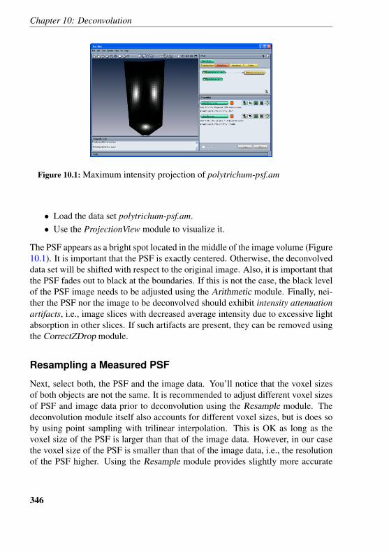
Chapter 10: Deconvolution
Figure 10.1: Maximum intensity projection of polytrichum-psf.am
• Load the data set polytrichum-psf.am.• Use the ProjectionView module to visualize it.
The PSF appears as a bright spot located in the middle of the image volume (Figure10.1). It is important that the PSF is exactly centered. Otherwise, the deconvolveddata set will be shifted with respect to the original image. Also, it is important thatthe PSF fades out to black at the boundaries. If this is not the case, the black levelof the PSF image needs to be adjusted using the Arithmetic module. Finally, nei-ther the PSF nor the image to be deconvolved should exhibit intensity attenuationartifacts, i.e., image slices with decreased average intensity due to excessive lightabsorption in other slices. If such artifacts are present, they can be removed usingthe CorrectZDrop module.
Resampling a Measured PSF
Next, select both, the PSF and the image data. You’ll notice that the voxel sizesof both objects are not the same. It is recommended to adjust different voxel sizesof PSF and image data prior to deconvolution using the Resample module. Thedeconvolution module itself also accounts for different voxel sizes, but is does soby using point sampling with trilinear interpolation. This is OK as long as thevoxel size of the PSF is larger than that of the image data. However, in our casethe voxel size of the PSF is smaller than that of the image data, i.e., the resolutionof the PSF higher. Using the Resample module provides slightly more accurate
346
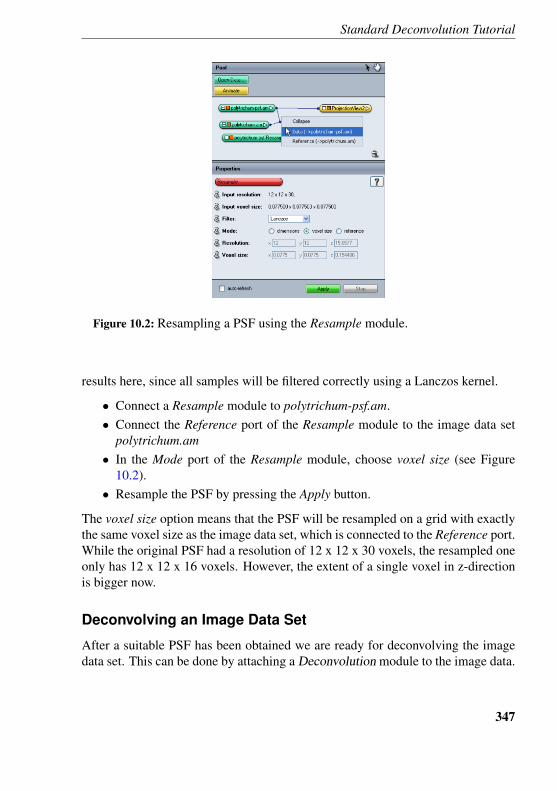
Standard Deconvolution Tutorial
Figure 10.2: Resampling a PSF using the Resample module.
results here, since all samples will be filtered correctly using a Lanczos kernel.
• Connect a Resample module to polytrichum-psf.am.• Connect the Reference port of the Resample module to the image data set
polytrichum.am• In the Mode port of the Resample module, choose voxel size (see Figure
10.2).• Resample the PSF by pressing the Apply button.
The voxel size option means that the PSF will be resampled on a grid with exactlythe same voxel size as the image data set, which is connected to the Reference port.While the original PSF had a resolution of 12 x 12 x 30 voxels, the resampled oneonly has 12 x 12 x 16 voxels. However, the extent of a single voxel in z-directionis bigger now.
Deconvolving an Image Data Set
After a suitable PSF has been obtained we are ready for deconvolving the imagedata set. This can be done by attaching a Deconvolution module to the image data.
347
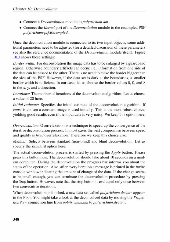
Chapter 10: Deconvolution
• Connect a Deconvolution module to polytrichum.am.• Connect the Kernel port of the Deconvolution module to the resampled PSF
polytrichum-psf.Resampled.
Once the deconvolution module is connected to its two input objects, some addi-tional parameters need to be adjusted (for a detailed discussion of these parameterssee also the reference documentation of the Deconvolution module itself). Figure10.3 shows these settings:
Border width: For deconvolution the image data has to be enlarged by a guardbandregion. Otherwise boundary artifacts can occur, i.e., information from one side ofthe data can be passed to the other. There is no need to make the border bigger thanthe size of the PSF. However, if the data set is dark at the boundaries, a smallerborder width is sufficient. In our case, let us choose the border values 0, 0, and 8in the x, y, and z direction.
Iterations: The number of iterations of the deconvolution algorithm. Let us choosea value of 20 here.
Initial estimate: Specifies the initial estimate of the deconvolution algorithm. Ifconst is chosen a constant image is used initially. This is the most robust choice,yielding good results even if the input data is very noisy. We keep this option here.
Overrelaxation: Overrelaxation is a technique to speed up the convergence of theiterative deconvolution process. In most cases the best compromise between speedand quality is fixed overrelaxation. Therefore we keep this choice also.
Method: Selects between standard (non-blind) and blind deconvolution. Let usspecify the standard option here.
The actual deconvolution process is started by pressing the Apply button. Pleasepress this button now. The deconvolution should take about 10 seconds on a mod-ern computer. During the deconvolution the progress bar informs you about thestatus of the operation. Also, after every iteration a message is printed in the Amiraconsole window indicating the amount of change of the data. If the change seemsto be small enough, you can terminate the deconvolution procedure by pressingthe Stop button. However, note that the stop button is evaluated only once betweentwo consecutive iterations.
When deconvolution is finished, a new data set called polytrichum.deconv appearsin the Pool. You might take a look at the deconvolved data by moving the Projec-tionView connection line from polytrichum.am to polytrichum.deconv.
348
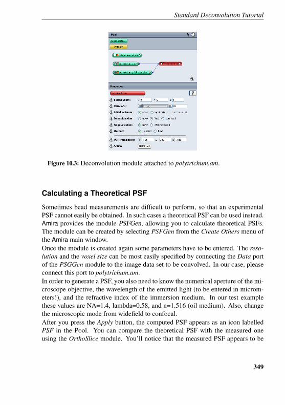
Standard Deconvolution Tutorial
Figure 10.3: Deconvolution module attached to polytrichum.am.
Calculating a Theoretical PSF
Sometimes bead measurements are difficult to perform, so that an experimentalPSF cannot easily be obtained. In such cases a theoretical PSF can be used instead.Amira provides the module PSFGen, allowing you to calculate theoretical PSFs.The module can be created by selecting PSFGen from the Create Others menu ofthe Amira main window.Once the module is created again some parameters have to be entered. The reso-lution and the voxel size can be most easily specified by connecting the Data portof the PSGGen module to the image data set to be convolved. In our case, pleaseconnect this port to polytrichum.am.In order to generate a PSF, you also need to know the numerical aperture of the mi-croscope objective, the wavelength of the emitted light (to be entered in microm-eters!), and the refractive index of the immersion medium. In our test examplethese values are NA=1.4, lambda=0.58, and n=1.516 (oil medium). Also, changethe microscopic mode from widefield to confocal.After you press the Apply button, the computed PSF appears as an icon labelledPSF in the Pool. You can compare the theoretical PSF with the measured oneusing the OrthoSlice module. You’ll notice that the measured PSF appears to be
349
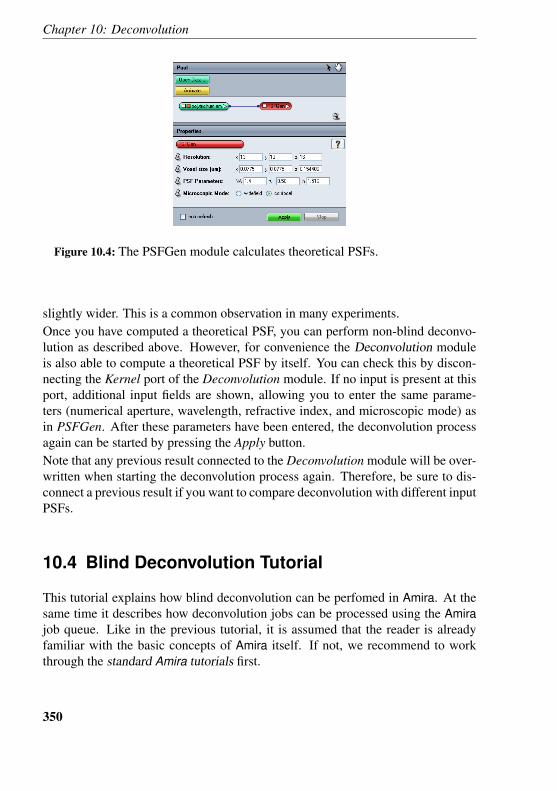
Chapter 10: Deconvolution
Figure 10.4: The PSFGen module calculates theoretical PSFs.
slightly wider. This is a common observation in many experiments.Once you have computed a theoretical PSF, you can perform non-blind deconvo-lution as described above. However, for convenience the Deconvolution moduleis also able to compute a theoretical PSF by itself. You can check this by discon-necting the Kernel port of the Deconvolution module. If no input is present at thisport, additional input fields are shown, allowing you to enter the same parame-ters (numerical aperture, wavelength, refractive index, and microscopic mode) asin PSFGen. After these parameters have been entered, the deconvolution processagain can be started by pressing the Apply button.Note that any previous result connected to the Deconvolution module will be over-written when starting the deconvolution process again. Therefore, be sure to dis-connect a previous result if you want to compare deconvolution with different inputPSFs.
10.4 Blind Deconvolution Tutorial
This tutorial explains how blind deconvolution can be perfomed in Amira. At thesame time it describes how deconvolution jobs can be processed using the Amirajob queue. Like in the previous tutorial, it is assumed that the reader is alreadyfamiliar with the basic concepts of Amira itself. If not, we recommend to workthrough the standard Amira tutorials first.
350
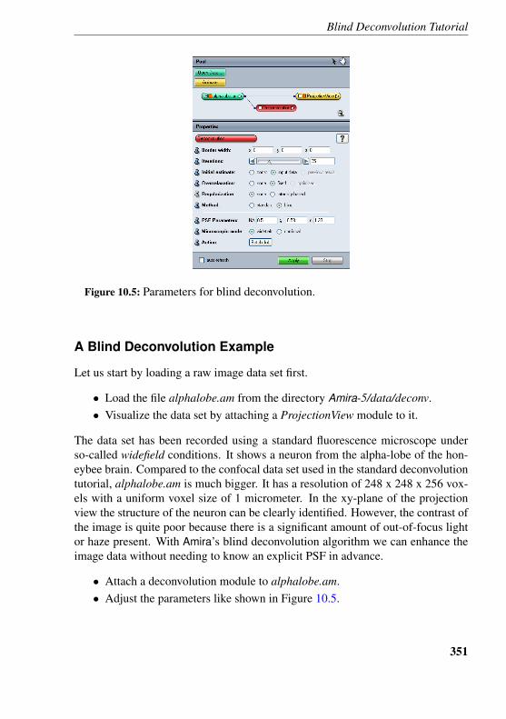
Blind Deconvolution Tutorial
Figure 10.5: Parameters for blind deconvolution.
A Blind Deconvolution Example
Let us start by loading a raw image data set first.
• Load the file alphalobe.am from the directory Amira-5/data/deconv.• Visualize the data set by attaching a ProjectionView module to it.
The data set has been recorded using a standard fluorescence microscope underso-called widefield conditions. It shows a neuron from the alpha-lobe of the hon-eybee brain. Compared to the confocal data set used in the standard deconvolutiontutorial, alphalobe.am is much bigger. It has a resolution of 248 x 248 x 256 vox-els with a uniform voxel size of 1 micrometer. In the xy-plane of the projectionview the structure of the neuron can be clearly identified. However, the contrast ofthe image is quite poor because there is a significant amount of out-of-focus lightor haze present. With Amira’s blind deconvolution algorithm we can enhance theimage data without needing to know an explicit PSF in advance.
• Attach a deconvolution module to alphalobe.am.• Adjust the parameters like shown in Figure 10.5.
351
Chapter 10: Deconvolution
The individual parameters have the following meaning:Border width: As for standard non-blind deconvolution, the image data has tobe enlarged by a guardband region. Otherwise boundary artifacts can occur, i.e.,information from one side of the data can be passed to the other. In our case weonly provide a small guardband region of 8 voxels in x- and y-direction. In z-direction we do not provide any border because there are sufficiently many emptyslices below and above the actual neuron. The resulting size of the data arrayson which the computations are performed then is 256 x 256 x 256. Because 256is a power of two (28), the Fast Fourier Transforms, the computationally mostexpensive part of the deconvolution algorithm, can be executed somewhat faster.Iterations: We choose a value of 25 here. Depending on the data, usually at least10 iterations are required. With overrelaxation being enabled (see below), resultsusally don’t improve much after 40 iterations.Initial estimate: Specifies the initial estimate of the deconvolution algorithm.Since there is not much noise present in the original alphalobe images it is safeto chose input data here. This causes the algorithm to converge even faster.Overrelaxation: Overrelaxation is a technique to speed up the convergence of theiterative deconvolution process. We enable overrelaxation by chosing the fixedtoggle.Regularization: We chose none here in order to do no regularization.Method: We chose blind here in order to select the blind deconvolution algorithm.PSF Parameters: For alphalobe.am the numerical aperture is 0.5, the wavelengthis 0.58 micrometers, and the refractive index is 1.33 (water). These parametersare required in order to apply certain constraints to the estimated point spreadfunction. They are also used in order to compute an initial PSF. If a data set wouldbe connected to the Kernel port of the deconvolution module, this data set wouldbe used as the inital PSF with the given PSF parameters still acting as constraints.For example, you could provide a measured PSF and let it be fitted to the actualdata by the deconvolution algorithm.Microscopic mode: alphalobe.am is a widefield data set, so select this option here.
Submitting a Deconvolution Job
After all parameters have been entered, the deconvolution process can be started.On a modern computer, blind deconvolution of our test data set roughly takes about20 minutes. Especially, if you want to deconvolve multiple data sets at once it isinconvenient to do this in an interactive session. Therefore multiple deconvolution
352
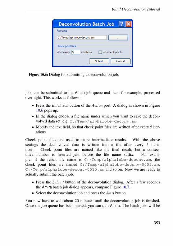
Blind Deconvolution Tutorial
Figure 10.6: Dialog for submitting a deconvolution job.
jobs can be submitted to the Amira job queue and then, for example, processedovernight. This works as follows:
• Press the Batch Job button of the Action port. A dialog as shown in Figure10.6 pops up.
• In the dialog choose a file name under which you want to save the decon-volved data set, e.g. C:/Temp/alphalobe-deconv.am.
• Modify the text field, so that check point files are written after every 5 iter-ations.
Check point files are used to store intermediate results. With the abovesettings the deconvolved data is written into a file after every 5 itera-tions. Check point files are named like the final result, but a consec-utive number is inserted just before the file name suffix. For exam-ple, if the result file name is C:/Temp/alphalobe-deconv.am, thecheck point files are named C:/Temp/alphalobe-deconv-0005.am,C:/Temp/alphalobe-deconv-0010.am and so on. Now we are ready toactually submit the batch job.
• Press the Submit button of the deconvolution dialog. After a few secondsthe Amira batch job dialog appears, compare Figure 10.7.
• Select the deconvolution job and press the Start button.
You now have to wait about 20 minutes until the deconvolution job is finished.Once the job queue has been started, you can quit Amira. The batch jobs will be
353
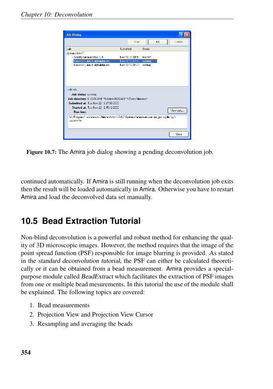
Chapter 10: Deconvolution
Figure 10.7: The Amira job dialog showing a pending deconvolution job.
continued automatically. If Amira is still running when the deconvolution job exitsthen the result will be loaded automatically in Amira. Otherwise you have to restartAmira and load the deconvolved data set manually.
10.5 Bead Extraction Tutorial
Non-blind deconvolution is a powerful and robust method for enhancing the qual-ity of 3D microscopic images. However, the method requires that the image of thepoint spread function (PSF) responsible for image blurring is provided. As statedin the standard deconvolution tutorial, the PSF can either be calculated theoreti-cally or it can be obtained from a bead measurement. Amira provides a special-purpose module called BeadExtract which facilitates the extraction of PSF imagesfrom one or multiple bead mesurements. In this tutorial the use of the module shallbe explained. The following topics are covered:
1. Bead measurements2. Projection View and Projection View Cursor3. Resampling and averaging the beads
354
Bead Extraction Tutorial
Bead Measurements
The PSF is the image of a single point source recorded under the same conditionsas the actual specimen. It can be approximated by the image of a fluorescing sub-resolution microsphere, a so-called bead. Performing good bead measurementsrequires some practice and expertise. In order to obtain good results the followinghints should be obeyed:
1. Use appropriate beads. It is important that the bead size be smallerthan approximately 1/2 full width at half maximum (FWHM) of thePSF. Good sources for obtaining beads suitable for PSF measurementsare Molecular Probes (http://www.probes.com/) or Polysciences(http://www.polysciences.com/).
2. The beads must be solid. Besides solid beads, there are also beads with theshape of a spherical shell, allowing to check the focus plane of a mircoscope.Such beads cannot be used as a source for PSF generation in the currentversion of Amira.
3. Don’t record clusters of multiple beads. Sometimes multiple beads mayglue together, appearing as a single big bright spot. Computing a PSF fromsuch a spot obviously leads to wrong results.
4. Note that beads are not resistant to a variety of embedding media. In par-ticular beads will be destroyed in xylene-based embedding media such asPermount (Fisher Scientific) and methyl salicylate (frequently used to clearup the tissue). As a substitute you might use immersion oil instead, whichhas a refractive index similar to methyl salicylate, for example.
5. Sample and beads should always be imaged as close to the coverslip aspossible. When it is not possible to attach the sample to the coverslip, thebeads should also be imaged in a comparable depth, embedded in the samemounting medium. Imaging the beads with better quality than the samplewill yield a slightly blurred deconvolution result. However, when the PSFused for deconvolution is too wide, artifacts can arise during deconvolution.
The objective lense should always be selected according to the mountingmedium, i.e. if the sample is attached to the slide and embedded in a bufferof refractive index close to water, a severe loss of image quality can be ex-pected when using an oil-immersion objective without a correction collar.Deconvolution of properly imaged data will allways be supperior to decon-volution of data suffering from aberrations.
355
Chapter 10: Deconvolution
6. Problems occur if the mounting medium remains liquid. In that case thesample distribution may not be permanent. If your specimen is to be em-bedded in water, you can try to immerse the beads in an agarose gel ofmoderate concentration instead. Attaching the small beads to the coverslip(for example by letting them dry) is often also sufficient for immobilization.
An example of an image data set containing multiple beads is provided in the filebeads.am in the directory Amira-5/data/deconv.
• Load the data set beads.am.• Visualize the data using a ProjectionView module.
Projection View and Projection View Cursor
The bead data set contains five different beads which can be clearly seen in thethree orthogonal planes of the ProjectionView module. In order to obtain a singlePSF we first want to select several ”good” beads. These beads are then resampledand averaged, thus yielding the final PSF. A bead can be considered as ”good”if it is clearly visible and if it is not superimposed by other beads (even whendefocused),Selecting ”good” beads is an interactive process. It is most easily accomplishedusing the ProjectionView’s Cursor module. This module allows you to select apoint in 3D space by clicking on one of the three planes of the ProjectionViewmodule. The third coordinate is automatically set by looking for the voxel withthe highest intensity. Points selected with the Cursor module can be stored in aLandmarkSet data object.
• Attach a Cursor module to the ProjectionView module.• Click on any bead on one of the three planes.• Store the current cursor position in a LandmarkSet object by pressing the
Add button.• Select and add some other beads too.
The landmarks need not to be located exactly at the center of a bead. The exactcenter positions can be fitted automatically later on.You can remove incorrect bead positions from the landmark set by invoking thelandmark set editor. In order to activate the editor, select the landmark set objectand press Landmark Editor button. If you want to add additional bead positions to
356
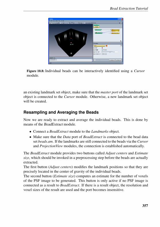
Bead Extraction Tutorial
Figure 10.8: Individual beads can be interactively identified using a Cursormodule.
an existing landmark set object, make sure that the master port of the landmark setobject is connected to the Cursor module. Otherwise, a new landmark set objectwill be created.
Resampling and Averaging the Beads
Now we are ready to extract and average the individual beads. This is done bymeans of the BeadExtract module.
• Connect a BeadExtract module to the Landmarks object.• Make sure that the Data port of BeadExtract is connected to the bead data
set beads.am. If the landmarks are still connected to the beads via the Cursorand ProjectionView modules, the connection is established automatically.
The BeadExtract module provides two buttons called Adjust centers and Estimatesize, which should be invoked in a preprocessing step before the beads are actuallyextracted.The first button (Adjust centers) modifies the landmark positions so that they areprecisely located in the center of gravity of the individual beads.The second button (Estimate size) computes an estimate for the number of voxelsof the PSF image to be generated. This button is only active if no PSF image isconnected as a result to BeadExtract. If there is a result object, the resolution andvoxel sizes of the result are used and the port becomes insensitive.
357
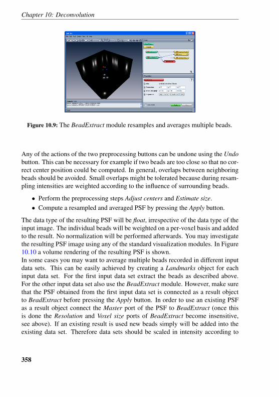
Chapter 10: Deconvolution
Figure 10.9: The BeadExtract module resamples and averages multiple beads.
Any of the actions of the two preprocessing buttons can be undone using the Undobutton. This can be necessary for example if two beads are too close so that no cor-rect center position could be computed. In general, overlaps between neighboringbeads should be avoided. Small overlaps might be tolerated because during resam-pling intensities are weighted according to the influence of surrounding beads.
• Perform the preprocessing steps Adjust centers and Estimate size.• Compute a resampled and averaged PSF by pressing the Apply button.
The data type of the resulting PSF will be float, irrespective of the data type of theinput image. The individual beads will be weighted on a per-voxel basis and addedto the result. No normalization will be performed afterwards. You may investigatethe resulting PSF image using any of the standard visualization modules. In Figure10.10 a volume rendering of the resulting PSF is shown.In some cases you may want to average multiple beads recorded in different inputdata sets. This can be easily achieved by creating a Landmarks object for eachinput data set. For the first input data set extract the beads as described above.For the other input data set also use the BeadExtract module. However, make surethat the PSF obtained from the first input data set is connected as a result objectto BeadExtract before pressing the Apply button. In order to use an existing PSFas a result object connect the Master port of the PSF to BeadExtract (once thisis done the Resolution and Voxel size ports of BeadExtract become insensitive,see above). If an existing result is used new beads simply will be added into theexisting data set. Therefore data sets should be scaled in intensity according to
358
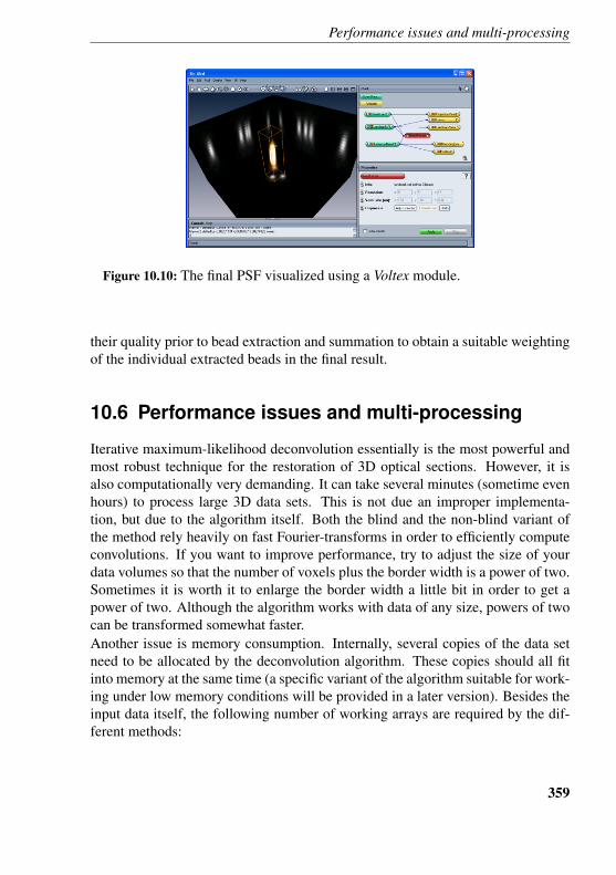
Performance issues and multi-processing
Figure 10.10: The final PSF visualized using a Voltex module.
their quality prior to bead extraction and summation to obtain a suitable weightingof the individual extracted beads in the final result.
10.6 Performance issues and multi-processing
Iterative maximum-likelihood deconvolution essentially is the most powerful andmost robust technique for the restoration of 3D optical sections. However, it isalso computationally very demanding. It can take several minutes (sometime evenhours) to process large 3D data sets. This is not due an improper implementa-tion, but due to the algorithm itself. Both the blind and the non-blind variant ofthe method rely heavily on fast Fourier-transforms in order to efficiently computeconvolutions. If you want to improve performance, try to adjust the size of yourdata volumes so that the number of voxels plus the border width is a power of two.Sometimes it is worth it to enlarge the border width a little bit in order to get apower of two. Although the algorithm works with data of any size, powers of twocan be transformed somewhat faster.Another issue is memory consumption. Internally, several copies of the data setneed to be allocated by the deconvolution algorithm. These copies should all fitinto memory at the same time (a specific variant of the algorithm suitable for work-ing under low memory conditions will be provided in a later version). Besides theinput data itself, the following number of working arrays are required by the dif-ferent methods:
359
Chapter 10: Deconvolution
• 3 working arrays for the non-blind algorithm with no or with fixed overre-laxation
• 5 working arrays for the non-blind algorithm with optimized overrelaxation• 5 working arrays for the blind algorithm
The number of voxels of a working array is the product of the number of voxels ofthe input data set plus the border with along each spatial dimension. The primitivedata type of a working array is a 4-byte floating point number. For example, if thenumber of voxels of the input data set plus the border width is 256 x 256 x 256 (asfor the alphalobe.am data set in the blind deconvolution tutorial), each workingarray will be about 64 MB, irrespective of the primitive data type of the input dataset. Therefore at least 192 MB (3x4x256x256x256 bytes) are required for non-blind deconvolution with fixed overrelaxation, and 320 MB (5x4x256x256x256bytes) for blind deconvolution. Keep this in mind when configuring the computeron which to perform deconvolution! However, also note that for most platforms itusually doesn’t make sense to have more than 1.5 GB of main memory. For morememory a 64-bit operating system is required.Finally, it should be mentioned that the deconvolution algorithm can make useof a multi-processor CPU board. Although you do not get twice the perfor-mance on a dual-processor PC, a speed-up of almost 1.5 can be achieved. Bydefault, Amira uses as many processors as there are on the computer. If forsome reason you want to use less processors you can set the environment vari-able AMIRA DECONV NUM THREADS to the number of processors you actuallywant to use simultaneously.
Example 1: Confocal Data
The original data set is provided under Amira-5/data/deconv/polytrichum.am. Theimages below were created using the ProjectionView module.The properties of the data set are as follows:
• Numerical aperture 1.4• Wavelength of the emitted light 0.58 micrometers• Refractive index 1.516 (oil)
360
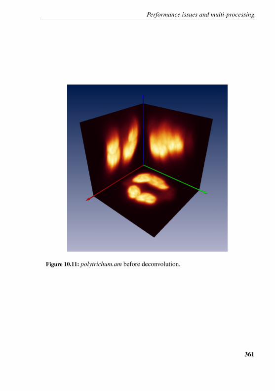
Performance issues and multi-processing
Figure 10.11: polytrichum.am before deconvolution.
361
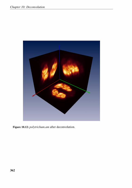
Chapter 10: Deconvolution
Figure 10.12: polytrichum.am after deconvolution.
362
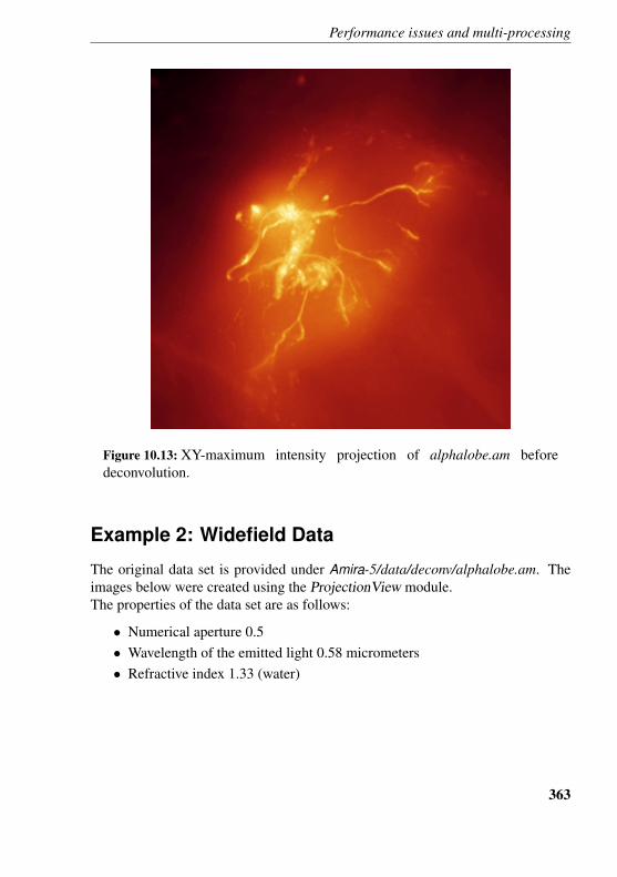
Performance issues and multi-processing
Figure 10.13: XY-maximum intensity projection of alphalobe.am beforedeconvolution.
Example 2: Widefield Data
The original data set is provided under Amira-5/data/deconv/alphalobe.am. Theimages below were created using the ProjectionView module.The properties of the data set are as follows:
• Numerical aperture 0.5• Wavelength of the emitted light 0.58 micrometers• Refractive index 1.33 (water)
363
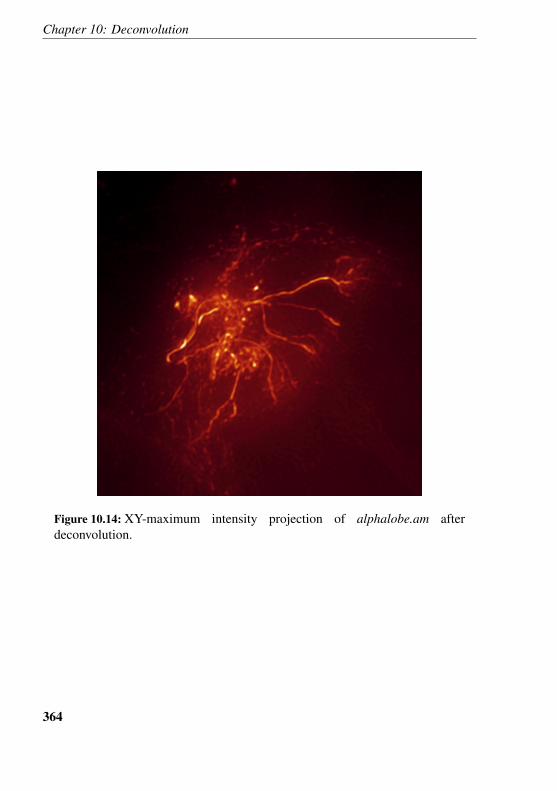
Chapter 10: Deconvolution
Figure 10.14: XY-maximum intensity projection of alphalobe.am afterdeconvolution.
364
11 Working with Multi-ChannelImages
This is a step-by-step tutorial on how to visualize multi-channel image data. Tofollow this tutorial you should be familiar with the basic concepts of Amira. Inparticular you should be able to load files, to interact with the 3D viewer, and toconnect display modules to data modules. All these issues are discussed in thegetting started section.We are going to load a set of multi-channel images into the workspace, attach aMultiChannelField group object to the data, and visualize it with several displaymodules. The steps are:
1. Load data into Amira.2. Create a MultiChannelField and attach channels to it.3. Using OrthoSlice with a MultiChannelField.4. Using ProjectionView with a MultiChannelField.5. Using Voltex with a MultiChannelField.6. Saving multi-channel images in a single AmiraMesh file.
11.1 Loading Multi-Channel Images into Amira
The data we will be working with in this tutorial are confocal stacks of the pro-thoracic ganglion of the locust Locusta migratoria. They were kindly provided byDr. Paul Stevenson, University of Leipzig, Germany. Two different channels wererecorded and stored as separate files.Amira supports a number of proprietary multi-channel formats of several micro-scope manufacturers (e.g., Leica and Zeiss). In such formats all channels are storedin a single file. Therefore the first steps described in this tutorial, namely groupingthe channels manually, can often be omitted.
365
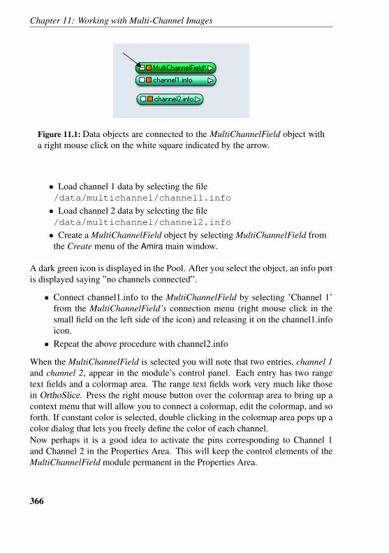
Chapter 11: Working with Multi-Channel Images
Figure 11.1: Data objects are connected to the MultiChannelField object witha right mouse click on the white square indicated by the arrow.
• Load channel 1 data by selecting the file/data/multichannel/channel1.info
• Load channel 2 data by selecting the file/data/multichannel/channel2.info
• Create a MultiChannelField object by selecting MultiChannelField fromthe Create menu of the Amira main window.
A dark green icon is displayed in the Pool. After you select the object, an info portis displayed saying ”no channels connected”.
• Connect channel1.info to the MultiChannelField by selecting ’Channel 1’from the MultiChannelField’s connection menu (right mouse click in thesmall field on the left side of the icon) and releasing it on the channel1.infoicon.
• Repeat the above procedure with channel2.info
When the MultiChannelField is selected you will note that two entries, channel 1and channel 2, appear in the module’s control panel. Each entry has two rangetext fields and a colormap area. The range text fields work very much like thosein OrthoSlice. Press the right mouse button over the colormap area to bring up acontext menu that will allow you to connect a colormap, edit the colormap, and soforth. If constant color is selected, double clicking in the colormap area pops up acolor dialog that lets you freely define the color of each channel.Now perhaps it is a good idea to activate the pins corresponding to Channel 1and Channel 2 in the Properties Area. This will keep the control elements of theMultiChannelField module permanent in the Properties Area.
366
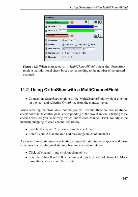
Using OrthoSlice with a MultiChannelField
Figure 11.2: When connected to a MultiChannelField object the OrthoSlicemodule has additional check boxes corresponding to the number of connectedchannels.
11.2 Using OrthoSlice with a MultiChannelField
• Connect an OrthoSlice module to the MultiChannelField by right clickingon the icon and selecting OrthoSlice from the context menu.
When selecting the OrthoSlice module, you will see that there are two additionalcheck boxes in its control panel corresponding to the two channels. Clicking thesecheck boxes lets you selectively switch on/off each channel. First, we adjust theintensity mapping of each channel separately.
• Switch off channel 2 by deselecting its check box.• Enter 23 and 200 in the min and max range fields of channel 1.
As a result, weak stainings – potentially unspecific staining – disappear and thosestructures that exhibit good staining become even more intense.
• Click off channel 1 and click on channel two.• Enter the values 8 and 200 in the min and max text fields of channel 2. Move
through the slices to see the results.
367
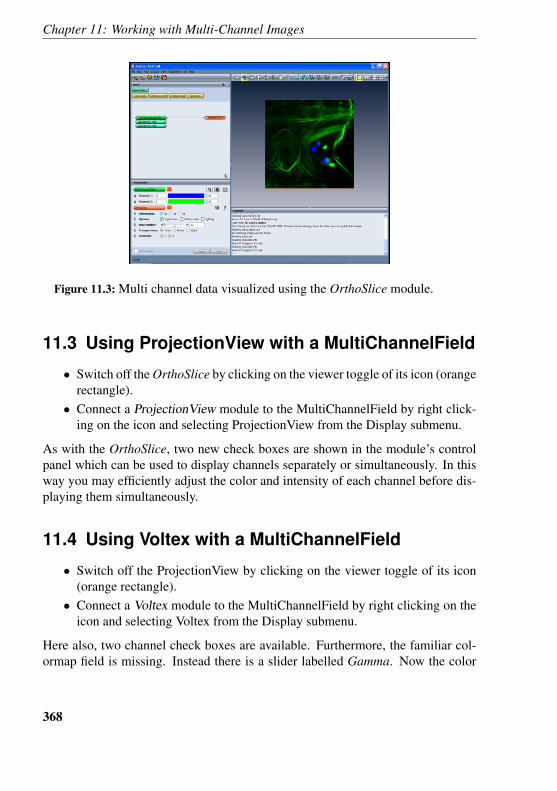
Chapter 11: Working with Multi-Channel Images
Figure 11.3: Multi channel data visualized using the OrthoSlice module.
11.3 Using ProjectionView with a MultiChannelField
• Switch off the OrthoSlice by clicking on the viewer toggle of its icon (orangerectangle).
• Connect a ProjectionView module to the MultiChannelField by right click-ing on the icon and selecting ProjectionView from the Display submenu.
As with the OrthoSlice, two new check boxes are shown in the module’s controlpanel which can be used to display channels separately or simultaneously. In thisway you may efficiently adjust the color and intensity of each channel before dis-playing them simultaneously.
11.4 Using Voltex with a MultiChannelField
• Switch off the ProjectionView by clicking on the viewer toggle of its icon(orange rectangle).
• Connect a Voltex module to the MultiChannelField by right clicking on theicon and selecting Voltex from the Display submenu.
Here also, two channel check boxes are available. Furthermore, the familiar col-ormap field is missing. Instead there is a slider labelled Gamma. Now the color
368
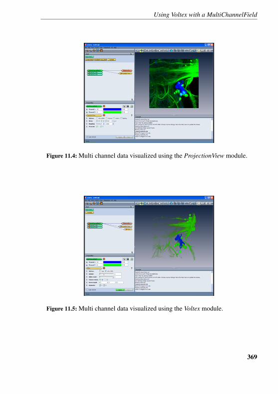
Using Voltex with a MultiChannelField
Figure 11.4: Multi channel data visualized using the ProjectionView module.
Figure 11.5: Multi channel data visualized using the Voltex module.
369
Chapter 11: Working with Multi-Channel Images
of each channel is determined by that defined in the MultiChannelField and theGamma slider controls the steepness of the alpha value (opacity) mapping usedfor volume rendering. Because volume rendering makes intensive use of hardwaretexture mapping and most consumer graphics adapters are limited in texture mem-ory size, it is recommended to enter at least factors of 2 2 1 in the Downsampletext fields of the Voltex module.
• Press the Apply button.
Each time you want to display another channel, you must press the Apply buttonagain.
11.5 Saving a MultiChannelField in a SingleAmiraMesh File
When the MultiChannelField icon is selected in the Pool, choose Save Data Asfrom the File menu, enter a filename, and click OK. The data will be stored inAmiraMesh format so that each time you load the data the two channel stacks andthe MultiChannelField group object will be restored.
370

Part VII
Skeleton Option User’s Guide
371

12 Skeleton Option User’s Guide
This is a step-by-step tutorial on how to use Large Disk Data to analyze micro-vascular networks in human brain tissue. Please note that another tutorial is avail-able to learn how to extract filament networks from vessels or neuron images. Tofollow this tutorial you should be familiar with the basic concepts of Amira. Inparticular you should be able to load files, to interact with the 3D viewer, and toconnect display modules to data modules. All these issues are discussed in thegetting started section.We are going to load 4 overlapping bricks of a large data set. The goal is to mergethese bricks into one large volume (Large Disk Data). The volume will be storedon disk only – subvolumes can be loaded into memory. Some basic operations candirectly be applied to the large volume.For the tutorial you should have access to a directory to which you’re allowed towrite files.We don’t provide any TIFF data with this tutorial. Hopefully you have a couple ofblocks (AmiraMesh format) to test the algorithm on. Generally it is a good idea toimport them into Amira and specify an approximate bounding box near the correctposition.
12.1 Importing your Image Data
You should have your image data as stacks of numbered 2D images. The topmostslice should have the lowest number. File formats recognized by Amira can befound in the File Formats section of the user’s guide. A good choice is TIFF be-cause it provides lossless compression and is readable on many different systems.You should also know the position in 3D of the lower left front corner of the brickyou’re going to import and the voxel size.Choose File/Open Data.... A File Dialog pops up. You can now select all of the2D images comprising the brick. After you press Load, another dialog pops up:
373
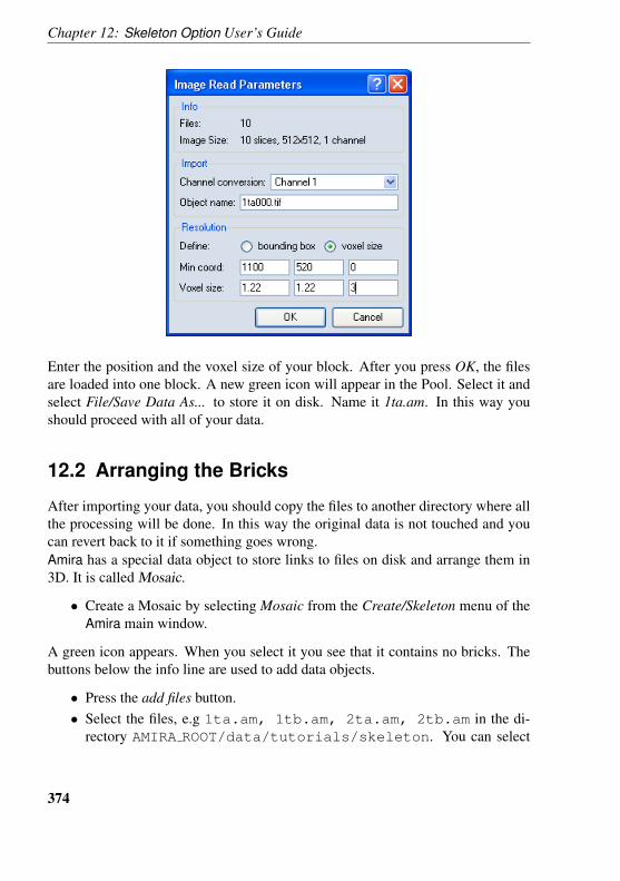
Chapter 12: Skeleton Option User’s Guide
Enter the position and the voxel size of your block. After you press OK, the filesare loaded into one block. A new green icon will appear in the Pool. Select it andselect File/Save Data As... to store it on disk. Name it 1ta.am. In this way youshould proceed with all of your data.
12.2 Arranging the Bricks
After importing your data, you should copy the files to another directory where allthe processing will be done. In this way the original data is not touched and youcan revert back to it if something goes wrong.Amira has a special data object to store links to files on disk and arrange them in3D. It is called Mosaic.
• Create a Mosaic by selecting Mosaic from the Create/Skeleton menu of theAmira main window.
A green icon appears. When you select it you see that it contains no bricks. Thebuttons below the info line are used to add data objects.
• Press the add files button.• Select the files, e.g 1ta.am, 1tb.am, 2ta.am, 2tb.am in the di-
rectory AMIRA ROOT/data/tutorials/skeleton. You can select
374
Aligning Bricks
multiple files at once by clicking on the first one and shift clicking on thelast one.
• Press Load.
The selected files are added to the Mosaic. The Info port shows the overall numberof the bricks added up to now. You can visualize the bricks with the DisplayMosaicmodule.
• Create a DisplayMosaic module by right clicking on the Mosaic and select-ing Skeleton/DisplayMosaic from the context menu.
• Select the yellow DisplayMosaic icon and switch the highlighted brick bydragging the slider in the interaction area.
• Save the Mosaic.
12.3 Aligning Bricks
A special module allows to exactly align the bricks based on their gray values.
• Attach an AlignBlocks module to the Mosaic by selecting Skele-ton/AlignBlocks in the data context menu.
• If you saved the mosaic already, its filename appears in Mosaic name.• Press the Apply button to start the processing.
A maximum intensity projection (mip) of each block is computed. These mips arealigned and the resulting transformations are applied to the bricks on disk.
12.4 Filtering, Correcting Z-Drop, Resampling
It is possible to apply the same operation to all the bricks at once. To do this youmust create a template for this operation. This could either be one brick with aneditor (e.g. Digital Image Filters) attached or a compute module (e.g. Resample).We’re going to demonstrate these two examples now. But first we should correctfor the Z-Drop:
• Load one brick of the mosaic by using the File/Open Data... menu.• Attach a Deconv/CorrectZDrop module to the brick.• Press Apply to start the correction procedure and check the result.
375
Chapter 12: Skeleton Option User’s Guide
• Attach an ApplyTemplateToMosaic script object by right clicking on theMosaic and selecting ApplyTemplate from the Skeleton submenu in the con-text menu.
• Attach the Template connection of the ApplyTemplateToMosaic module tothe CorrectZDrop module.
• Select ApplyTemplateToMosaic and press Apply.
Next we’re going to apply a digital filter to all blocks:
• Load one brick of the mosaic by using the File/Open Data... menu.• Select the data icon of the brick.• Attach a Digital Image Filter by pressing the Digital Filters button in the
Properties Area.• Select Gauss from the Filter port, and apply it. To check the results you can
attach an OrthoSlice.• Attach the Template connection of the ApplyTemplateToMosaic module to
the filter object (with the data attached).• Select ApplyTemplateToMosaic and press Apply.
Another useful filter might be Median2D or the Median3D. For Median3D, selectMedian from the first pulldown menu of the Filter port, and 3D from the secondpulldown menu. The application of the latter filter takes some time but leads togood results.The script object starts to load each brick of the mosaic, applies the filter to it,and writes it back to the same location on disk. There are no warnings about thisoverwrite.In the next step we’re going to resample every brick to an isotropic voxel size. Thisis only an optional step and might lead to smoother central lines in the followingprocessing. But it increases size of the data on disk by a factor of about three. Youshould carefully consider whether you want to perform this step or not.
• Attach a Resample module to the brick loaded before and select Mode: voxelsize and adjust Voxel size: z to get an isotropic result.
• Press Apply to start the resampling procedure and check the result.• Attach the Resample module to the Template connection of the ApplyTem-
plateToMosaic module.• Press Apply of the ApplyTemplateToMosaic module.
376
Creating the Large Disk Data
All bricks are resampled and saved to the same position. It is a good idea to sampleall bricks to an isotropic voxel size. It improves the result of the distance map andthe skeletonization we’re going to apply.As a standard prefiltering procedure you should:
• Apply the ZDropCorrection.• Apply a 2D median filter.• Apply a 3D Gaussian filter with a small sigma (1 or smaller).
If the results are not satisfactory, you should try to extend the prefiltering step.
12.5 Creating the Large Disk Data
The next step is to create a new Large Disk Data object and sample the bricks ontoit. The overlapping regions can be blended with each other and a border can beadded.Note: The thinning algorithm expects a black border around the data. The bordershould be at least of size lenOfEnds used during thinning (see below). By defaulta border of 15 voxels on each side in each dimension. Be sure to check this if youmanually set lenOfEnds.
• Attach a MosaicToLargeDiskData to the Mosaic by right clicking on theMosaic and selecting Skeleton/MosaicToLargeDiskData from the submenuin the context menu.
• Select the red MosaicToLargeDiskData icon.
You can see some options in the Properties Area. The default options are fine forthe tutorial.
• A default filename derived from the mosaic is displayed in the Filenameport. You might want to override it.
• Press the Apply button.
A new green icon which represents the new data object will appear in the Pool.After this the bricks will be loaded one after the other and will be sampled. Thismay take some time.
• Select the new green icon (titled Image).
In the Properties Area some information about the data stored on disk is displayed.Next,
377
Chapter 12: Skeleton Option User’s Guide
• Delete or switch off the DisplayMosaic module.• Connect a BoundingBox to the Mosaic icon.• Connect a BoundingBox to the Image icon.
The second box is slightly bigger than the bounding box of the Mosaic. This isdue to the border added by the MosaicToLargeDiskData module.
12.6 Accessing the Large Disk Data
You can’t directly visualize the Large Disk Data by e.g. attaching an OrthoSlice.Before you can do this, you must select a subvolume and load this subvolume intothe Pool. The Subvolume will be an ordinary Amira field and you can use all themodules that you normally use. It may be a good idea to clean up the Pool now,but it’s not required. The Mosaic is no longer needed.
• Connect an LatticeAccess to the Image object by right clicking on it andselecting LatticeAccess from the popup menu.
• Select the red LatticeAccess icon.
In the viewer you can see a dragger box in one corner of the bounding box of theLarge Disk Data. You can click and drag the corners or the faces of the box tospecify the subvolume you want to load. In the Properties Area the correspondingdimensions are displayed.
• Drag the box somewhere inside the volume (For this you need to switch theviewer into interaction mode).
• Press the Apply button.• Attach an OrthoSlice to the new green icon (Image.view).• Select the LatticeAccess object, then toggle on the auto-refresh check box.• Drag the box in the viewer.
By setting auto-refresh on, every time you drag the box an automatic reload isstarted and all modules downstream of the view are recomputed. This is an easyway to scan through the large volume. Try different display modules on the Im-age.view, e.g., an isosurface.
378
Computing directly on the Large Disk Data
12.7 Computing directly on the Large Disk Data
Some computation modules are able to handle the Large Disk Data directly. Theseinclude thresholding, computation of a distance map, thinning, extracting a line setfrom a voxel skeleton, and computation of the thickness of the lines (evaluatingthe distance map at the points of the lineset). All these steps are presented in thissubsection.The first step is to apply a simple thresholding.
• Attach a Threshold to the Image icon by right clicking on it and selectingThreshold from the Skeleton submenu in the popup menu.
• Select an appropriate threshold in the Properties Area.• Select a filename you want to store the result to. In the tutorial we will use
the default name Image.labels.• Press the Apply button.
A new green icon that contains the labels will appear. Connect an LatticeAccessmodule to it as described above and have a look at the results.You might want to correct the result of the segmentation procedure manually. Thismight be useful to fill big vessels or remove uninteresting parts. Amira has a seg-mentation editor to perform this task. Due to the size of the data, you will have towork on subblocks of the whole data set.In the next step we’ll calculate a distance map of the object.
• Attach a ChamferMap to the Image.labels icon by right clicking on it andselecting ChamferMap from the Skeleton submenu in the popup menu.
• Specify an filename (the default is OK for the tutorial).• Press Apply.
A new green icon named Image.dm will appear. Connect an LatticeAccess moduleand have a look at the distance map.The thinning procedure needs the labels and the distance map as input.Note: The thinning algorithm automatically detects endpoints of vessels. A pa-rameter is used to distinguish them from ”noise” on the surface of the vessels toavoid spurious branches. You might want to change this parameter manually inthe console. Use Thinner setVar lenOfEnds 10 to set the length of theends to 10 voxels before they are detected as unconnected ends. This is a ratherlarge value leading to only a few branches. The drawback is that you also mightmiss real endpoints. It will be really hard to detect such errors during the network
379
Chapter 12: Skeleton Option User’s Guide
check. But in general we think it is a good idea to avoid spurious branches directlyduring thinning.
• Attach a Thinner to the Image.labels icon by right clicking on it and select-ing Thinner from the Skeleton submenu in the popup menu.
• Connect the port for the distance map to the Image.dm icon. You can achievethis by right clicking on the white square on the left side of the ExtThinnericon and selecting Distmap. A blue line is attached to the mouse pointer;after you click on the Image.dm icon, the two modules are connected.
• Specify a filename (the default is fine for the tutorial).• Press Apply.
A new green icon named Image.thinned will appear and the thinning process isstarted. It may take some time before it finishes. We will directly go on andconvert the result into a lineset before visualizing it.
• Attach a TraceLines to the Image.thinned icon by right clicking on it andselecting TraceLines from the Skeleton submenu in the popup menu.
• Unselect the cluster toggle in the Properties Area.• Press Apply.
The new icon that is visible now in the Pool is a lineset, which you are probablyalready familiar with. You can visualize it by connecting a LineSetView.
• Create an LineSetView module by right clicking on the Image.lineset andselecting LineSetView from the context menu.
The lines are rather jaggy because they connect centers of voxels. To get smootherlines you can use a Tcl command in the console.
• Type Image.lineset smooth into the Amira console window. Youcan repeat this if you would prefer even smoother lines.
You can use the CheckNetwork module from the Skeleton submenu in the contextmenu to remove short ends.In the last step of this subsection we will compute a thickness for every point onthe lines. For the thickness we use the values of the distance map.
• Attach an EvalOnLines to the Image.lineset icon by right clicking on it andselecting EvalOnLines from the Compute submenu in the popup menu.
380
Region of Interest
• Connect the port for the distance map to the Image.dm icon. You can achievethis by right clicking on the white square on the left side of the EvalOnLinesicon and selecting Field. A blue line is attached to the mouse pointer; afteryou click on the Image.dm icon, the two modules are connected.
• Press Apply.
The module doesn’t create a new data icon. It is more like an editor and changes theconnected lineset. It adds a data value for every vertex in the lineset and calculatesthe value of the field at the point of the vertex. You can visualize the data with theLineSetView.
• Select the LineSetView by clicking on it.• In the Properties Area there is a drop down menu called ColorMode. Click
on it and select Data 0.• Right click on the rectangular area in the row Colormap. A popup menu
appears. Select physics.icol.• Change the range of the colormap by clicking into text field right of the
colormap and type in 15.
You see that the lines are now colored. The color is an indicator for the local radiusof the original object.
12.8 Region of Interest
During visualization of large data sets there is often the need to restrict the dis-played geometry to a subvolume of the total data set. It would be nice if differentmodules shared the same volume and the volume could be changed simultaneouslyfor all of them. In Amira there is a special module that provides this possibility;it is called SelectRoi. You can attach it to every spatial data object. Some dis-play modules have a connection called ROI that can be attached to the SelectRoimodule to restrict the view.
• Remove all objects except for the Image.lineset and the LineSetView.• Create a SelectRoi module by right clicking on the Image.lineset and select-
ing SelectRoi from the Display submenu of the context menu.• Connect the Connection named ROI of the LineSetView to the SelectRoi
module. To do this, right click on the white square on the left side ofthe LineSetView icon and select ROI. A blue line is attached to the mouse
381
Chapter 12: Skeleton Option User’s Guide
pointer; after you click on the SelectRoi icon, the two modules are con-nected.
• Switch the viewer to interaction mode and click and drag one of the greensquares. This will adjust the Region of Interest and the LineSetView willadopt the new restriction immediately.
• By clicking and dragging on the (invisible) faces of the cuboid you can moveit to another position.
When working with a small subset of the lineset, it is possible to do more involvedvisualizations that require more graphics power. For example, the lines can bedisplayed as tubes that reflect the local thickness.
• Choose a rather small part of the lineset.• Select the LineSetView.• Click on the Shape drop down menu and select Circle.• Click on the ScaleMode drop down menu and select Data 0.• Move the ScaleFactor slider to 2.
In the viewer the lines are now displayed as tubes. The thickness is scaled with thedata associated with the lines.Note: The data value associated with the lines is the local radius. The LineSetViewscales by the local diameter. To scale to the physical size you therefore must use aScaleFactor of 2.In the next step we’re going to load a part of the image data that is also determinedby the SelectRoi module. You can then easily load the same subvolume from dif-ferent lda files if you connect all LatticeAccess modules to one common SelectRoimodule.
• Load the file Image that you saved before.• Attach an LatticeAccess module to it (see above if you don’t know how).• Connect the Connection named ROI of the LatticeAccess to the SelectRoi
module. This is done the same way as with the LineSetView.• Select the LatticeAccess module, then press the Apply button.• Attach a ProjectionView display module to the newly displayed green Im-
age.view icon.• You can do the same for the Image.labels file.
382
Check Network
All LatticeAccess modules you created are now restricted to the same volume andcan easily be moved by one click-and-drag operation.
12.9 Check Network
In this subsection we’d like to present a module that can be used to jump to allendpoints of a lineset and create some nice views for checking if the endpoints arefine or if they should be edited.
• Create a CheckNetwork module by right clicking on the Image.lineset andselecting CheckNetwork from the Skeleton submenu of the popup menu.
• Connect the SelectRoi connection of the CheckNetwork to the SelectRoimodule (right click on the white square at the left of CheckNetwork, selectSelectRoi, click on the yellow SelectRoi icon).
• Select the LatticeAccess module, and toggle on the auto-refresh check box.• Adjust the size of the lines by selecting the LineSetView and changing the
ScaleFactor slider to approximately 0.15.• Select the CheckNetwork module.• Press the Next Endpoint button.• By repeating the last step you can jump through all endpoints.
12.10 Coloring a Lineset According to its DepthValue
It can be useful to color the lines in different ways. In the next example we’regoing to color the lineset by the local z value. This is done in two steps:
• Create a Scalarfield which provides the depth (z value).• Evaluate this value on the lines and use a LineSetView.
To create the Scalarfield:
• Select Create/Data/Scalarfield.• Select the newly created icon.• Type z into the Expr field.
383

Chapter 12: Skeleton Option User’s Guide
The next step it to evaluate this scalarfield on the lineset. You can do this byselecting the lineset and typing into the console.Hint: Press the <TAB> key to get the name of the selected module.
• Type lines computeData scalarfield 2 to evaluate the data(Fill in your specific names for lines and scalarfield). The 2 in-dicates to store the data values as data 2 in the lineset.
• Attach a LineSetView and use data2 for color coding.
384
Index
.Amira, 161, 200Amira
class structure, 148data objects, 4modules, 4Options, 13
Amira SEG-Y Reader, 14Amira Developer Option, 13Amira DICOM reader, 13Amira Mesh Option, 13Amira Molecular Option, 13Amira Quantification+ Option, 14Amira Skeleton Option, 14Amira Very Large Data Option, 14Amira Virtual Reality Option, 14Amira.init, 161, 200Microscopy Option, 13AMIRA LOCAL, 161, 184AMIRA ROOT, 184
abberation, 355affine transformations, 153agarose gel, 356alignment, 62AMD64 architecture, 162auto-save, 142auto-select modules, 141axial blur, 342
batch job, 353bead extraction, 354beads, 355black level, 344border width, 348, 352boundary artifacts, 343bounding box, 25
camera trackball, 131CATIA 4, 14CATIA 5, 14check point files, 353color depth, 163command line options, 158commands, 185compute indicator, 141confocal microscope, 342, 344coordinates, 151coverslip, 355Create menu, 114cropping, 32cross-section, 62CT, 58
data import, 157database
default, 111user-defined, 111
deconvolution
385
Index
blind, 342, 350non-blind, 342standard, 345
default directories, 160driver, 162
Edit menuCopy, 111Cut, 110Database, 111Delete, 111Paste, 111Preferences, 112Select All, 111
editors, 4embedding medium, 355environment variables, 159Explorer, 124
F1 key, 184features, 4file dialog
changing directories, 138filename filter, 138popup menu, 139selecting files, 138
File menuJobs, 110Open data, 107Open Time Series, 108Quit, 110Recent Files, 110Recent Networks, 110Save Data, 108Save Data As, 108Save Network, 109
firing algorithm, 141flow visualization, 69
font size, 161, 162Fourier transform, 359function key, 162
procedure, 200fusion, 58
hardware, 162help
for commands, 184help browser, 118searching, 120
hidden data objects, 142hot-key procedure, 162, 200
IGES, 14immersion medium, 355in-plane sampling, 344initial estimate, 348, 352intensity attenuation, 346isosurface, 32
job dialog, 353Job dialog box, 139
LabelField, 40Lanczos filter, 347landmark, 53LargeDiskData, 26Linux system, 162load, 26
Mac system, 162maximum-likelihood method, 342Mecalog Radioss For Amira, 14memory consumption, 359microsphere, 355modalities, 58model, 47MRT, 58
386

Index
multi-processing, 360
noise, 342, 344numerical aperture, 344Nyquist sampling, 343
oil immersion, 355OpenGL, 162OpenGL driver, 163optical sectioning microscopy, 342out-of-focus light, 342, 351overrelaxation, 348, 352oversampling, 344
parameters of data objects, 154particle plot, 69performance, 359PET, 58Pool, 122Pool menu
Auto adjust range of col-ormaps, 114
Duplicate, 113Duplicate mode, 114Hide, 112Remove, 112Remove All, 113Rename, 113Show, 113Show All, 113
Port, 121preferences, 141processor, 162PSF, 342, 345
theoretical, 349
reampling, 347refracrtive index, 355refractive index, 344
registration, 58regular grid, 151
sampling rate, 343saturation, 344save network, 142, 199scalar fields, 150scanned volume, 343script, 182SCRIPTDIR, 184SCRIPTFILE, 184scripting, 182Scripting interface, 175segmentation, 40Shadowing, 154simulation, 47Snapshot dialog box, 146Spacemouse, 161stacked slices, 26start-up script, 161, 200STEP, 14stereo mode, 161stream lines, 69stream visualization, 69sub-application concept, 155surface, 152swap space, 163system information dialog, 147system requirements
development, 162Linux, 164Mac, 165Windows, 164
TCL, 182Tcl, 175Tcl introduction, 176tetrahedral grid, 47
387
Index
tetrahedral grids, 152TNO Madymo For Amira, 14Tracker Emulator, 322troubleshooting, 163tutorials, 17
undersampling, 344
vector field visualization, 69vector fields, 151VertexSets, 153View menu
Axis, 117Background, 115Console, 117Easy fade, 117Fading effect, 117Fog, 116FPS (frames-per-second), 117Frame counter, 117Layout, 115Lights, 116Measuring, 117Transparency, 115
Viewer, 131camera trackball, 131Fullscreen, 135Home, 134Interact, 133interaction mode, 132Layout, 135Measuring, 135Perspective/Ortho toggle, 134Pick, 133rotate button , 133Seek, 133Set Home, 134Snapshot, 135
Stereo, 135Trackball, 133Translate, 133View, 133View All, 134viewing directions Axial, Coro-
nal, Sagittal, 134viewing directions YZ, XZ,
XY, 134viewing mode, 132Zoom, 133zoom, 131
viewer toggles, 141virtual memory, 163virtual reality, 265volume rendering, 32
warping, 53wavelength, 344widefield data, 343Windows system, 162work area, 129
388

Related Documents