Design and Construction of an Optical Polarimeter for the Study of Ice-like Analogs using Near Zero Phase Angle Measurements Mrunal Amin A Thesis submitted to the Faculty of Graduate Studies in Partial Fulfillment of the Requirements for the Degree of Masters of Science Graduate Program in Science York University Toronto, Ontario September 2018 ©Mrunal Amin, 2018

Welcome message from author
This document is posted to help you gain knowledge. Please leave a comment to let me know what you think about it! Share it to your friends and learn new things together.
Transcript
Design and Construction of an Optical Polarimeter for the Study of Ice-like
Analogs using Near Zero Phase Angle Measurements
Mrunal Amin
A Thesis submitted to the Faculty of Graduate Studies in Partial Fulfillment of the
Requirements for the Degree of
Masters of Science
Graduate Program in Science
York University
Toronto, Ontario
September 2018
©Mrunal Amin, 2018
Abstract
Previous studies for analog samples measuring polarized backscatter near zero phase an-
gles have suggested strong presence of multiple scattering effects. Radar data for Mercury,
Moon and other icy Galilean satellites exhibit high circular polarization ratios with de-
creasing phase angle that indicates the possible presence of icy deposits in the polar
craters. An examination of powder samples with known composition and grain sizes was
undertaken to try and further understand the interaction of polarized light with closely
packed particulate medium. The goal of this research was to construct and test a long
arm Goniometric optical instrument capable of measuring polarization ratios in the range
from 0-5 degree phase angle for understanding and differentiating the scattering effects
that occur near zero phase angle. Measuring signal intensity and circular polarization
ratios with the newly setup optical polarimeter for various analog samples will provide
a framework for understanding the characteristics of embedded scatterers within the icy
regoliths.
ii

Dedication
Dedicated to my grandparents and parents who taught me I could do anything I put my
mind to, And to Mansi, for being there to remind me they were right
iii
Acknowledgments
First and foremost, with immense gratitude I would like to thank the help of my super-
visor Professor Michael Daly, Associate Professor in the Department of Earth and Space
Science and Engineering and co-supervisor Professor Regina Lee, Associate Professor in
the Department of Earth and Space Science and Engineering at York University, as well as
their steadfast support over the course of this project. I would like to thank Dr. David T.
Blewett, Applied Physics Laboratory at John Hopkins University for providing previous
data, analog samples and continuous support throughout the research.
To all my fellow colleagues, I would like to convey my deepest appreciation for all the
support and encouragement throughout my project. I am highly grateful to Kati Bal-
achandran, Undergraduate at York University for all the help assembling the instrument.
Special thanks to Amy Shaw for teaching and guiding me on the Goniometric instrument.
I would like to express my gratitude to all my teachers at York University who put
their faith in me and urged me to do better.
iv

Table of Contents
Abstract ii
Dedication iii
Acknowledgments iv
Table of Contents v
List of Figures ix
List of Tables xiii
1 Introduction 1
1.1 Historical Summary . . . . . . . . . . . . . . . . . . . . . . . . . . . . . . . 1
1.2 Research Context . . . . . . . . . . . . . . . . . . . . . . . . . . . . . . . . 2
1.3 Research Objectives . . . . . . . . . . . . . . . . . . . . . . . . . . . . . . . 4
2 Theoretical Background 6
2.1 Stokes Parameters . . . . . . . . . . . . . . . . . . . . . . . . . . . . . . . 6
2.2 Polarization Ratio . . . . . . . . . . . . . . . . . . . . . . . . . . . . . . . . 8
2.2.1 Linear Polarization Ratio . . . . . . . . . . . . . . . . . . . . . . . . 8
2.2.2 Circular Polarization Ratio . . . . . . . . . . . . . . . . . . . . . . . 10
2.2.3 Examples of Polarization Ratios . . . . . . . . . . . . . . . . . . . . 11
2.3 Mueller Matrix . . . . . . . . . . . . . . . . . . . . . . . . . . . . . . . . . 17
v

2.3.1 Examples of Mueller Matrices for Optical Components . . . . . . . 19
2.4 Opposition Effects . . . . . . . . . . . . . . . . . . . . . . . . . . . . . . . 22
2.4.1 Shadow Hiding Opposition Effect . . . . . . . . . . . . . . . . . . . 23
2.4.2 Coherent Backscattering Effect . . . . . . . . . . . . . . . . . . . . 24
2.4.3 Properties of SHOE and CBOE . . . . . . . . . . . . . . . . . . . . 25
2.4.4 Detecting Ice Regoliths . . . . . . . . . . . . . . . . . . . . . . . . . 27
3 Techniques Deployed for Measuring Data 29
3.1 Measuring Stokes Parameters . . . . . . . . . . . . . . . . . . . . . . . . . 29
3.1.1 Rotating Quarter Wave Plate Technique . . . . . . . . . . . . . . . 29
3.2 Measuring Mueller Matrix . . . . . . . . . . . . . . . . . . . . . . . . . . . 31
3.2.1 Dual Rotating Quarter Wave Plate Technique . . . . . . . . . . . . 31
4 Instrumentation and Data Acquisition Procedures 34
4.1 Measurement Procedure . . . . . . . . . . . . . . . . . . . . . . . . . . . . 34
4.2 Multi-Axis Goniometric Instrument . . . . . . . . . . . . . . . . . . . . . . 38
4.2.1 Caddy Platform . . . . . . . . . . . . . . . . . . . . . . . . . . . . . 39
4.2.2 Arm Platform . . . . . . . . . . . . . . . . . . . . . . . . . . . . . . 41
4.3 Data Acquisition Setup . . . . . . . . . . . . . . . . . . . . . . . . . . . . . 44
4.3.1 Motor Control . . . . . . . . . . . . . . . . . . . . . . . . . . . . . . 45
4.3.2 Detector Control . . . . . . . . . . . . . . . . . . . . . . . . . . . . 46
4.3.3 Goniometer Control . . . . . . . . . . . . . . . . . . . . . . . . . . . 49
4.4 Data Acquisition Procedure . . . . . . . . . . . . . . . . . . . . . . . . . . 50
4.4.1 Sample Preparation . . . . . . . . . . . . . . . . . . . . . . . . . . . 53
4.4.2 Liquid Samples . . . . . . . . . . . . . . . . . . . . . . . . . . . . . 57
5 Measurements and Dataset Analysis 59
5.1 Previous Studies Observing Circular Polarization Ratios . . . . . . . . . . 59
5.2 Analog Measurements . . . . . . . . . . . . . . . . . . . . . . . . . . . . . 63
5.2.1 Stokes Parameters . . . . . . . . . . . . . . . . . . . . . . . . . . . 63
vi

5.2.2 Spectralon Standard . . . . . . . . . . . . . . . . . . . . . . . . . . 67
5.2.3 Alumina Samples . . . . . . . . . . . . . . . . . . . . . . . . . . . . 71
5.2.4 Signal Intensity for Spectralon and Alumina Samples . . . . . . . . 74
5.2.5 Liquid Samples . . . . . . . . . . . . . . . . . . . . . . . . . . . . . 76
5.3 Mueller Matrix Measurements . . . . . . . . . . . . . . . . . . . . . . . . . 80
5.3.1 Spectralon CPR trends with Mueller Matrix Correction . . . . . . . 83
5.3.2 Alumina CPR trends with Mueller Matrix Correction . . . . . . . . 86
6 Error Sources and Mitigation 88
6.1 Instrumentation Error . . . . . . . . . . . . . . . . . . . . . . . . . . . . . 88
6.1.1 Laser Beam Misalignment . . . . . . . . . . . . . . . . . . . . . . . 89
6.1.2 Stray Light Reflections . . . . . . . . . . . . . . . . . . . . . . . . . 91
6.1.3 Backscattering Losses . . . . . . . . . . . . . . . . . . . . . . . . . . 94
6.2 Calibration Error . . . . . . . . . . . . . . . . . . . . . . . . . . . . . . . . 96
6.2.1 Zeroing Goniometer Instrument . . . . . . . . . . . . . . . . . . . . 96
6.3 Measurement Error . . . . . . . . . . . . . . . . . . . . . . . . . . . . . . . 98
6.3.1 Detector Signal Stability . . . . . . . . . . . . . . . . . . . . . . . . 98
6.3.2 Motor Movement . . . . . . . . . . . . . . . . . . . . . . . . . . . . 99
6.4 Computation/Correction Error . . . . . . . . . . . . . . . . . . . . . . . . 100
6.4.1 Mueller Matrix Error . . . . . . . . . . . . . . . . . . . . . . . . . . 100
6.4.2 True Retardance Error . . . . . . . . . . . . . . . . . . . . . . . . . 103
6.4.3 Least Squares Estimate . . . . . . . . . . . . . . . . . . . . . . . . . 104
6.5 Error Analysis . . . . . . . . . . . . . . . . . . . . . . . . . . . . . . . . . . 105
7 Assessment of Analog Observations 107
8 Conclusion 111
9 Future Work 114
vii

Bibliography 117
Appendices 125
Appendix A Experimental Setup 126
Appendix B Stokes and Mueller Matrix Computation Code 128
viii
List of Figures
2.1 Schematic representation of a Left Handed Circularly Polarized Wave [32] . 7
2.2 Six polarization states of a light source represented with their respective
Irradiances for calculating the Stokes parameters [32] . . . . . . . . . . . . 8
2.3 Schematic representation of a Linearly polarized wave [32] . . . . . . . . . 9
2.4 Example of (A) 12.6 cm radar image of the southwestern Montes Cordillera
deposits of Orientale basin region. (B) Circular polarization ratio (C) De-
gree of linear polarization (D) Linear polarization angle [11] . . . . . . . . 13
2.5 An electromagnetic wave interacting with (a) single and (b) multiple cas-
cading optical systems with M, Mueller matrices.Ei and E0 indicates the
input and output polarization ellipse of the wave [32] . . . . . . . . . . . . 18
2.6 Change in polarization ellipse of an incoming radiation Ei when interacting
with an optical component represented by M, Mueller matrix [32] . . . . . 19
2.7 (a) Shadows cast by the particles from the sun are not visible to the observer
with Sun overhead, causing the area to appear brighter [15] (b) Example of
SHOE, taken by Apollo 17 astronaut Eugene Cernan on the lunar surface [30] 23
2.8 Schematic representation of the CBOE [1] . . . . . . . . . . . . . . . . . . 24
3.1 Schematic for the Rotating Quarter Wave Plate Technique [4] . . . . . . . 29
3.2 Dual Rotating Quarter Wave Plate Technique Schematic [20] . . . . . . . . 32
ix
4.1 Schematic of the setup for the optical system on the MAGI for near zero
phase angle measurements (Refer to Appendix A for distances between
optical components) . . . . . . . . . . . . . . . . . . . . . . . . . . . . . . 35
4.2 Optical components on the MAGI showing the propagation of the laser signal 36
4.3 Incoming and backscattered polarized signal from the sample platform on
the MAGI . . . . . . . . . . . . . . . . . . . . . . . . . . . . . . . . . . . . 37
4.4 Multi-Axis Goniometric Instrument used for near zero phase angle mea-
surements . . . . . . . . . . . . . . . . . . . . . . . . . . . . . . . . . . . . 38
4.5 Schematic of the optical components mounted on the caddy platform . . . 39
4.6 Schematic of the optical assembly on the arm platform . . . . . . . . . . . 41
4.7 Incident and Reflected beams propagating through the arm platform . . . 42
4.8 Schematic of the Data Acquisition Programs for the Optical Setup . . . . . 44
4.9 (a) The motor control software used to run the (b) Rotation stage where
the QWP was mounted . . . . . . . . . . . . . . . . . . . . . . . . . . . . . 45
4.10 Front panel display for the detector control software run through the Lockin
Amplifier . . . . . . . . . . . . . . . . . . . . . . . . . . . . . . . . . . . . . 47
4.11 Front panel display for the MAGI control software written in Labview en-
vironment . . . . . . . . . . . . . . . . . . . . . . . . . . . . . . . . . . . . 49
4.12 Block Diagram for the Optical Instrument control and interaction . . . . . 50
4.13 Flowchart for the Polarimetric Measurement Procedure . . . . . . . . . . . 51
4.14 Standard Spectralon Diffuse Samples from Labsphere . . . . . . . . . . . . 53
4.15 Microgrit Alumina powder prepared in a sample container . . . . . . . . . 55
4.16 Particle Size Distribution for 2.1 µm Alumina sample with Gamma and
Normal Probability Distribution Function . . . . . . . . . . . . . . . . . . 56
4.17 Liquid Solutions for Analog Measurements . . . . . . . . . . . . . . . . . . 57
5.1 Schematic from the Nelson’s experiment [37] . . . . . . . . . . . . . . . . . 60
5.2 CPR vs Phase Angle for highly reflective alumina sample from Nelson’s
experiment . . . . . . . . . . . . . . . . . . . . . . . . . . . . . . . . . . . . 61
x
5.3 Intensity values from the detector for 360°of quarter wave plate rotation . . 63
5.4 Four Fourier Coefficient values for 360°rotation of quarter wave plate . . . 64
5.5 Reflection model for Thermoplastic resin particles (Spectralon Pucks) [29] . 67
5.6 CPR vs Phase Angle for Standard Spectralon Diffuse Reflectance Pucks . . 69
5.7 CPR vs Phase Angle for Standard Spectralon Diffuse Reflectance Pucks . . 70
5.8 CPR vs Phase Angle for all Alumina Powdered Samples . . . . . . . . . . 72
5.9 Signal Intensity vs Phase Angle for Spectralon Samples . . . . . . . . . . . 74
5.10 Signal Intensity vs Phase Angle for Alumina Samples . . . . . . . . . . . . 75
5.11 Instrumentation setup for Liquid Samples . . . . . . . . . . . . . . . . . . 76
5.12 CPR vs Phase Angle for Glycerol+Alumina2.1µm with 10 and 15 Emer-
gence Angles . . . . . . . . . . . . . . . . . . . . . . . . . . . . . . . . . . . 77
5.13 Polystyrene Beads Suspension at 15 Emergence Angle . . . . . . . . . . . 78
5.14 Variations in the polarized signal propagating and reflecting from the beam
splitter . . . . . . . . . . . . . . . . . . . . . . . . . . . . . . . . . . . . . . 80
5.15 CPR vs Phase Angle for Standard Spectralon Diffuse Reflectance Pucks
with Mueller Matrix Correction. Dotted line shows the corrected values
while solid line shows the observed values . . . . . . . . . . . . . . . . . . . 83
5.16 CPR vs Phase Angle for Standard Spectralon Diffuse Reflectance Pucks
with Mueller Matrix Correction and Systematic errors. . . . . . . . . . . . 84
5.17 Alumina Powdered Samples with Mueller matrix correction. Dotted line
shows the corrected values while solid line shows the observed values. . . . 86
5.18 CPR vs Phase Angle for Alumina Powdered Samples with Systematic Errors 87
6.1 Offset Reflections resulting from Laser misalignment issues . . . . . . . . . 89
6.2 Offset Reflections propagating through incident and reflected beam paths
due to Laser misalignment . . . . . . . . . . . . . . . . . . . . . . . . . . . 90
6.3 Comparison between old and new analyzer mounting setup . . . . . . . . . 92
6.4 Stray light mitigation techniques employed in the instrumentation setup . . 93
6.5 Backscattering Intensities for different reflectors with standard sample pucks 94
xi
6.6 Caddy platform zero position with limited accuracy . . . . . . . . . . . . . 96
6.7 Rotation Stage Backlash Intensity Error . . . . . . . . . . . . . . . . . . . 99
6.8 Retardation errors ε1 and ε2, orientation errors ε3, ε4, ε5 from the dual
rotating retarder technique . . . . . . . . . . . . . . . . . . . . . . . . . . . 100
7.1 Reflectance vs Phase Angle for all Alumina Powdered Samples . . . . . . . 107
7.2 CPR vs Phase Angle for all Alumina Powdered Samples . . . . . . . . . . 108
7.3 CPR decrease near zero phase angle for alumina 2.1um grain size . . . . . 109
9.1 New beam splitter mounting technique . . . . . . . . . . . . . . . . . . . . 115
A.1 Optical Instrument Setup Schematic . . . . . . . . . . . . . . . . . . . . . 126
xii
List of Tables
2.1 Reflectance and CPR analog data for different grain sizes of Alumina sam-
ples observed by Nelson [38] . . . . . . . . . . . . . . . . . . . . . . . . . . 12
2.2 CPR values for interior and exterior Lunar crater regions from the LRO
mission [16] . . . . . . . . . . . . . . . . . . . . . . . . . . . . . . . . . . . 14
2.3 CPR vs Phase angle expected trends with decreasing phase angle for op-
position effects . . . . . . . . . . . . . . . . . . . . . . . . . . . . . . . . . 27
4.1 Components of the Optical Setup from Figure 4.1 . . . . . . . . . . . . . . 34
4.2 Caddy platform optical assembly components with their settings and func-
tions . . . . . . . . . . . . . . . . . . . . . . . . . . . . . . . . . . . . . . . 40
4.3 Optical components for the Arm platform with their settings and functions 43
4.4 Motor Control Software settings used for operating the rotation stage . . . 46
4.5 Lockin Amplifier Settings and functions for the detector control software . 48
5.1 CPR calculation from Fourier coefficients and Stokes parameters . . . . . . 65
5.2 Additional Polarization Parameters . . . . . . . . . . . . . . . . . . . . . . 66
5.3 Spectralon Diffuse Reflective Standard Samples . . . . . . . . . . . . . . . 68
5.4 Particle Size/Wavelength Comparison for Alumina Samples . . . . . . . . . 71
6.1 PDA100A Hi-Gain Detector Specifications . . . . . . . . . . . . . . . . . . 98
6.2 Alignment Errors from Mueller matrix calibration . . . . . . . . . . . . . . 102
6.3 Uncertainties from various sources . . . . . . . . . . . . . . . . . . . . . . . 106
xiii

7.1 Maximum and minimum CPR values from Alumina phase curves . . . . . 110
A.1 Distance between the optical components in the polarimeter assembly . . . 127
xiv

List of Acronyms
CBOE Coherent Backscattering Opposition Effect
CPR Circular Polarization Ratio
DOCP Degree of Circular Polarization
DOP Degree of Polarization
LHCP Left Handed Circular Polarization
LP Linear Polarizer
LPR Linear Polarization Ratio
LRO Lunar Reconnaissance Orbiter
MAGI Multi-Axis Goniometric Instrument
Mini-RF Miniature Radio Frequency
Nd:YAG Neodymium-Doped Yttrium Aluminum Garnet
NDF Neutral Density Filter
OC Opposite Circular Polarization state
QWP Quarter Wave Plate
RHCP Right Handed Circular Polarization
RQWP Rotating Quarter Wave Plate
SC Same Circular Polarization state
SHOE Shadow Hiding Opposition Effect
xv
1 Introduction
1.1 Historical Summary
Radar remote sensing is an important tool for probing the surface and sub-surface features
of Solar System bodies for possible presence of water ice. [10] Planetary radar techniques
have been able to differentiate radar scattering properties between dry/rocky surfaces of
inner Solar system bodies and their polar regions. Regions such as the poles of Mars,
polar craters of Mercury, Earth glaciers and icy Galilean satellites of Jupiter exhibit high
radar reflectivity compared to the low quasi-specular reflections from rough surfaces. [40]
The main differentiating factors present among the highly reflective radar data for polar
regions and rocky regions are the differences in the linear polarization ratios and circular
polarization ratios. Circular polarization ratio (CPR) indicates the difference in power
received in the same sense of polarization as incident versus the power received in the
opposite sense of polarization for the region under study. Linear polarization ratio (LPR)
is the ratio of the reflectance in the cross-polarized sense to that in the same-polarized
sense as incident. Single scattering causes a flip in the polarization state of the incident
signal, whereas multiple scattering tends to randomize the polarization state often causing
the return signal to be polarized in the same sense as incident. The differences in radar
data for polar and rocky regions are explained by observing polarization ratios for different
types of scattering. The most plausible explanation for high polarization ratios is volume
scattering within a weakly absorbing medium in which embedded scatterers are of the
sizes close to the radar wavelength. As ice weakly absorbs the incoming radiation at
planetary radar wavelengths the voids, cracks, density variations or rocks would act as
1

scatterers. Incident radiation on an icy surface with embedded scatterers would undergo
multiple scattering within the medium and emerge coherently to produce high reflectance
values. The coherent enhancement from such regions would occur at near zero phase angle
due to the opposition effects.
The presence of ice in the permanently shadowed crater regions of Mercury was con-
firmed from the radar bright, high CPR data collected by Slade and Butler. [9] The
thermal models from Paige [41] suggested that temperatures in the permanently shad-
owed regions of Mercury would be cold enough to trap volatiles over geological time
periods which were confirmed from polar topography data that are consistent with long
term retention of water ice. [41]. Further, active measurements of surface reflectance by
the laser altimeter reveal areas of high and low reflectance consistent with the presence
of surface ice in radar bright regions. Intuitively lunar shadowed polar regions would be
considered as favorable sites for possible presence of ice due to their distance from Sun but
the data is ambiguous. [31] Radar observations of lunar polar regions does not reveal areas
with strongly elevated returns and CPR similar to Mercury. Many groups have reported
studies of permanently shadowed polar regions that are visible to Earth based radar with
high CPR values, but they were found to occur both, within and outside the permanent
shadowed region. [19] [48] This raises the question whether rough, blocky ejecta or water
ice is responsible for CPR enhancement.
1.2 Research Context
The objective of this study is to conduct a series of optical scaled radar measurements
designed to explore key variables that contribute to the backscattering of electromagnetic
radiation from icy deposits. This can be achieved by examining the key differences in the
opposition effects for highly reflective analogs by observing reflectance and polarization
ratio trends.
Variables such as reflectance and circular polarization ratios for various planetary
bodies such as the Moon, Mars, Jupiter and Titan have been observed through radar
2
data. [40] [36] [27] Analog samples measuring the same variables have been observed from
0.05 - 5 degree phase angle range for highly reflective alumina samples. [37] Conducting
an experimental setup capable of measuring signal intensity and CPR values of analog
samples to an exact zero phase angle, would enable us to better understand the contri-
bution of opposition effects to the CPR and reflectance phase curves. The main goal
of this study is to construct a polarimeter capable of measuring polarized returns from
samples similar to that from previous studies and observe any discrepancies. With the
newly setup zero phase angle (defined as the angle between the observer, the observed
object and the incident light) polarimeteric instrument we can further analyze different
grain sizes of highly reflective and liquid samples. Polarized returns from polystyrene
beads suspended in a liquid medium will provide important information regarding the
size distribution of scatterers, number density of scatterers, absorption properties of the
medium and absorption properties of the scatterers.
Further work into mapping out the effects of scatters and the scattering medium will
provide a framework for interpreting planetary radar observations of ice-bearing and po-
tentially ice bearing deposits. This research will help constrain factors such as the purity of
ice and abundance, kind and size distribution of scatterers responsible for coherent effects.
Through this research we will be able to lay a platform for integrating laboratory results
from analog samples with mono and bistatic radar data for lunar polar regions acquired
by Mini-RF instrument [45] on the Lunar Reconnaissance Orbiter (LRO) spacecraft for
better understanding of the nature of lunar areas that may contain ice deposits. [47] [16]
Previous studies by Nelson and Hapke [37], [38], [23] involved measuring reflectance in
eight senses of polarization states and summing them to calculate the linear and circular
polarization ratios. In this research the Stokes parameter of the backscatter signal will
be calculated that provides all the information regarding the reflectance and polariza-
tion state of the signal. This method reduces the time taken for individual observations
allowing for precise polarization measurements.
3
1.3 Research Objectives
The primary objective of this research is to construct an experimental apparatus that is
capable of measuring signal intensity and polarization state of the backscattered signal
near zero phase angles. We will validate the constructed polarimeter by comparing ac-
quired data with previous analog data. The research will help us understand the polarized
backscatter returns for analog samples. This would allow future studies to constrain fac-
tors such as the purity of ice and the kind, abundance and size distribution of scatterers
responsible for high polarized near zero phase returns. Future work on integration of lab-
oratory analog data with mono and bistatic radar data for lunar polar regions collected by
the Mini-RF instrument on the LRO spacecraft would be highly beneficial. [45] [47]. The
research will allow for better understanding in the nature of lunar areas that may contain
ice and possibly help in re-interpreting published radar data for Mercurian deposits [9].
The key objectives to be achieved throughout this research are divided into primary and
secondary goals listed as follows.
Primary Objectives:
1. Design an optical platform capable of measuring off-axis polarized backscatter mea-
surements from analog samples.
2. Construct and re-iterate the design of the optical polarimeter to achieve objectives
3-6.
3. The instrument shall be capable of measuring the polarization state of the backscat-
ter.
4. The instrument shall be capable of taking measurements from 0-5 degree phase
angle.
4
5. The polarimeter shall be capable of acquiring measurements at exact zero phase
angle.
6. Important parameters such as Linear Polarization Ratio (LPR) and Circular Polar-
ization Ratio (CPR) shall be computed from the backscatter data.
7. Validate the constructed polarimeter by comparing CPR measurements with previ-
ous undertaken studies on analog samples.
Secondary Objectives:
1. Compute and observe CPR vs phase angle measurements for different analog sample
grain sizes.
2. Compute and observe signal intensity vs phase angle measurements for different
grain sizes.
3. Provide interpretations of the observed CPR and intensity phase curves.
4. Explore scattering effects responsible for backscattering from two different categories
of analog samples; powdered samples and suspended beads in a liquid medium.
5
2 Theoretical Background
The radar scattering properties of the icy satellites have been controversial for over a
decade as remote sensing remains the only way to obtain information about their surfaces.
The highly reflective radar backscattering properties of the icy satellites at zero phase
angles are associated with opposition effects namely Coherent Backscatter Opposition
Effect (CBOE) and the Shadow Hiding Opposition Effect (SHOE). The physical cause
for CBOE is due to the enhancement of radar brightness near zero phase angle by volume
scattering within a low-loss medium. The magnitude and shape of the opposition peak
depends on the properties of the surface such as particle size, porosity and scattering
behaviour of the individual regolith particles. There have been a number of studies
undertaken to determine the nature of opposition effects for icy analogs by observing the
polarization state of the backscattered signal. [23]
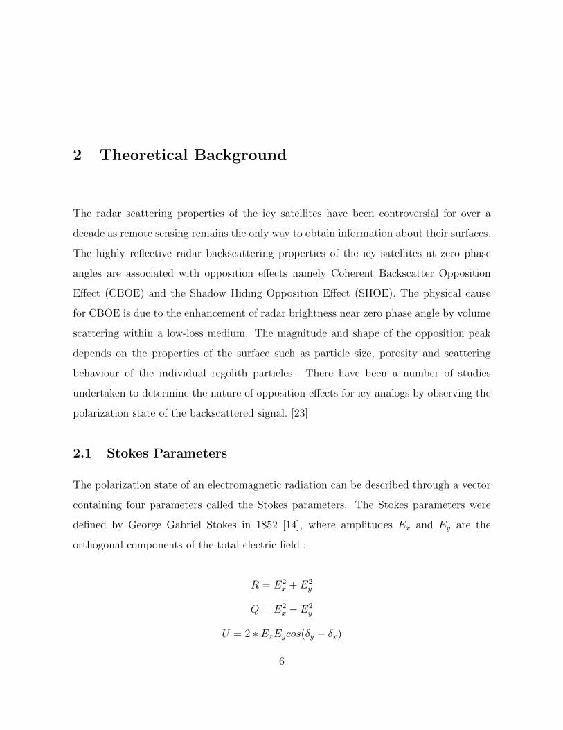
2.1 Stokes Parameters
The polarization state of an electromagnetic radiation can be described through a vector
containing four parameters called the Stokes parameters. The Stokes parameters were
defined by George Gabriel Stokes in 1852 [14], where amplitudes Ex and Ey are the
orthogonal components of the total electric field :
R = E2x + E2
y
Q = E2x − E2
y
U = 2 ∗ ExEycos(δy − δx)
6
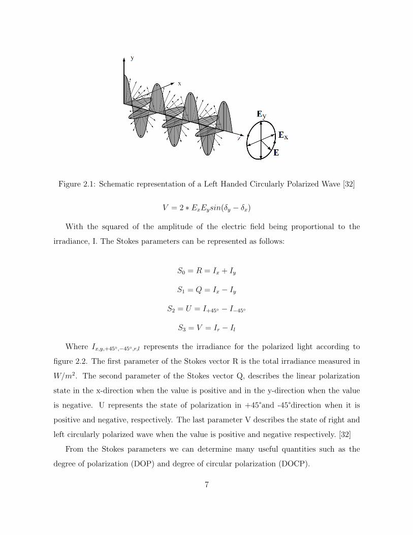
Figure 2.1: Schematic representation of a Left Handed Circularly Polarized Wave [32]
V = 2 ∗ ExEysin(δy − δx)
With the squared of the amplitude of the electric field being proportional to the
irradiance, I. The Stokes parameters can be represented as follows:
S0 = R = Ix + Iy
S1 = Q = Ix − Iy
S2 = U = I+45 − I−45
S3 = V = Ir − Il
Where Ix,y,+45,−45,r,l represents the irradiance for the polarized light according to
figure 2.2. The first parameter of the Stokes vector R is the total irradiance measured in
W/m2. The second parameter of the Stokes vector Q, describes the linear polarization
state in the x-direction when the value is positive and in the y-direction when the value
is negative. U represents the state of polarization in +45°and -45°direction when it is
positive and negative, respectively. The last parameter V describes the state of right and
left circularly polarized wave when the value is positive and negative respectively. [32]
From the Stokes parameters we can determine many useful quantities such as the
degree of polarization (DOP) and degree of circular polarization (DOCP).
7
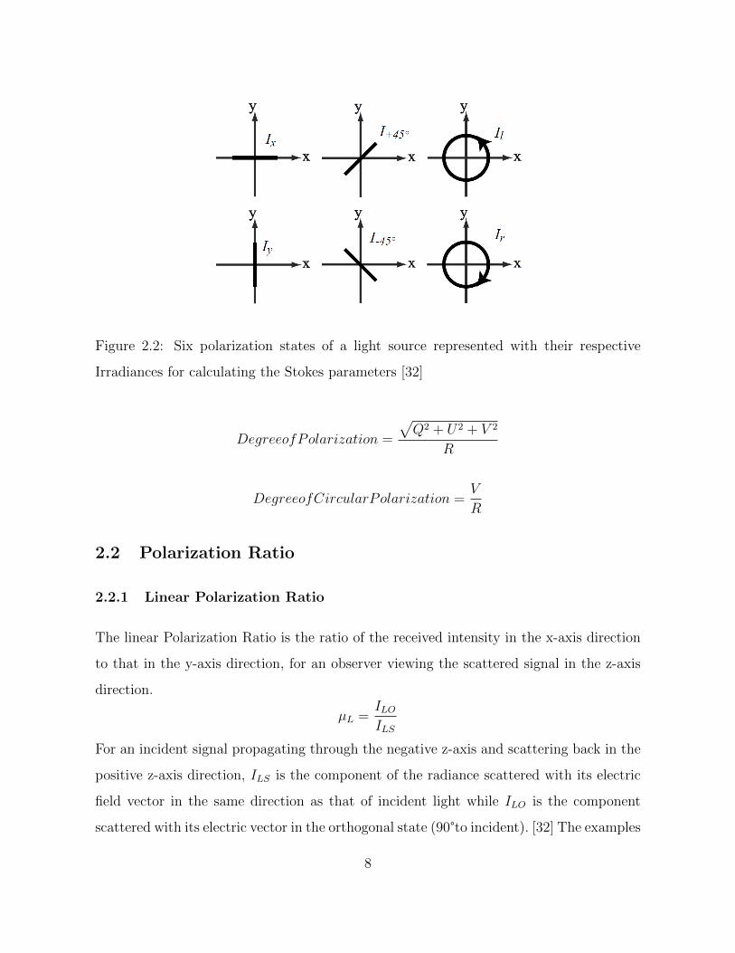
Figure 2.2: Six polarization states of a light source represented with their respective
Irradiances for calculating the Stokes parameters [32]
DegreeofPolarization =
√Q2 + U2 + V 2
R
DegreeofCircularPolarization =V
R
2.2 Polarization Ratio
2.2.1 Linear Polarization Ratio
The linear Polarization Ratio is the ratio of the received intensity in the x-axis direction
to that in the y-axis direction, for an observer viewing the scattered signal in the z-axis
direction.
µL =ILOILS
For an incident signal propagating through the negative z-axis and scattering back in the
positive z-axis direction, ILS is the component of the radiance scattered with its electric
field vector in the same direction as that of incident light while ILO is the component
scattered with its electric vector in the orthogonal state (90°to incident). [32] The examples
8
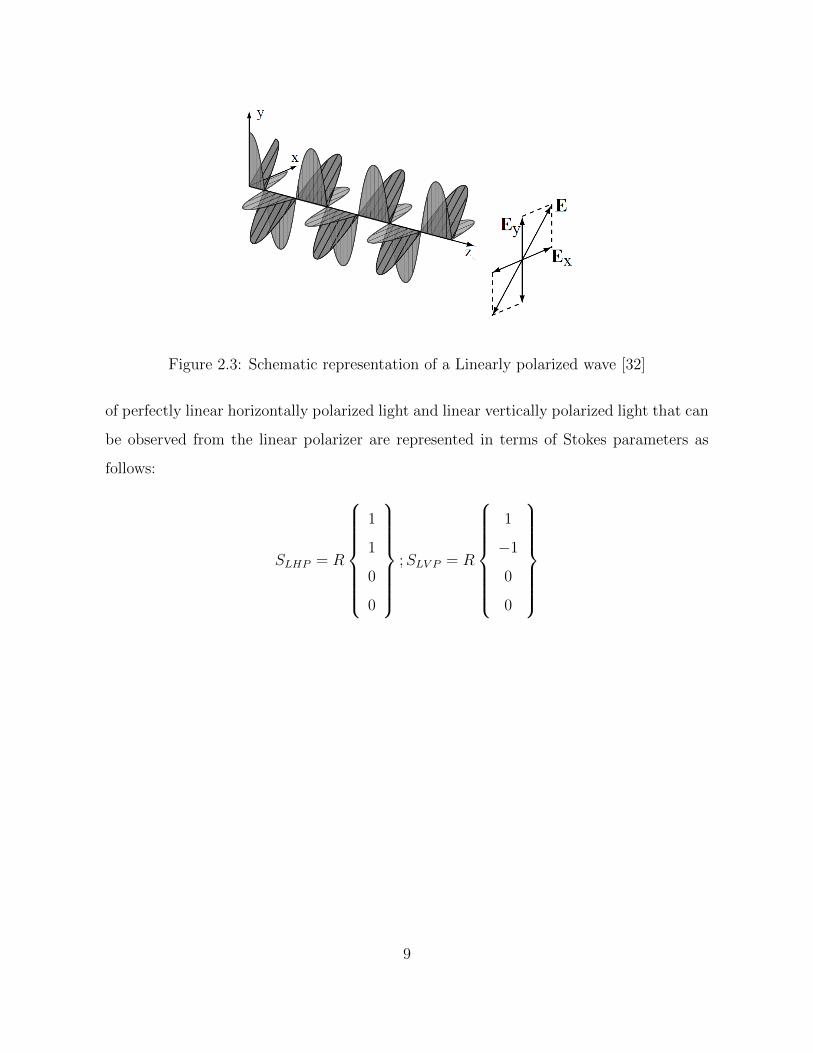
Figure 2.3: Schematic representation of a Linearly polarized wave [32]
of perfectly linear horizontally polarized light and linear vertically polarized light that can
be observed from the linear polarizer are represented in terms of Stokes parameters as
follows:
SLHP = R
1
1
0
0
;SLV P = R
1
−1
0
0
9
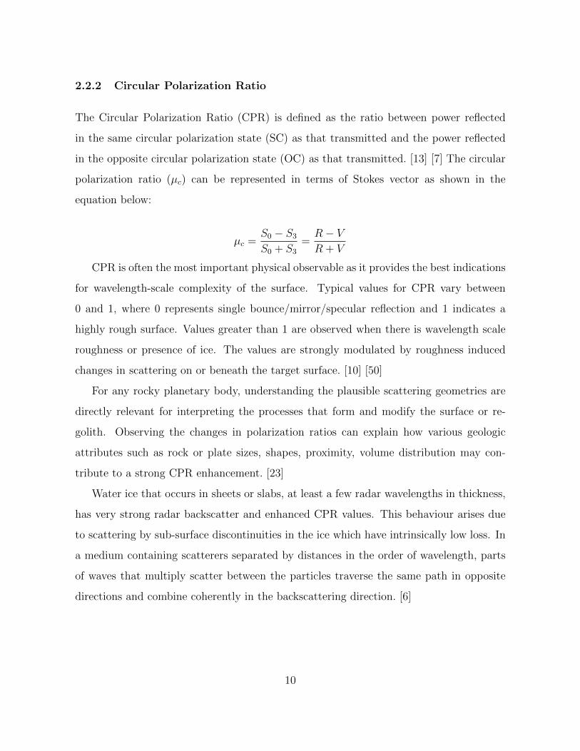
2.2.2 Circular Polarization Ratio
The Circular Polarization Ratio (CPR) is defined as the ratio between power reflected
in the same circular polarization state (SC) as that transmitted and the power reflected
in the opposite circular polarization state (OC) as that transmitted. [13] [7] The circular
polarization ratio (µc) can be represented in terms of Stokes vector as shown in the
equation below:
µc =S0 − S3
S0 + S3
=R− VR + V
CPR is often the most important physical observable as it provides the best indications
for wavelength-scale complexity of the surface. Typical values for CPR vary between
0 and 1, where 0 represents single bounce/mirror/specular reflection and 1 indicates a
highly rough surface. Values greater than 1 are observed when there is wavelength scale
roughness or presence of ice. The values are strongly modulated by roughness induced
changes in scattering on or beneath the target surface. [10] [50]
For any rocky planetary body, understanding the plausible scattering geometries are
directly relevant for interpreting the processes that form and modify the surface or re-
golith. Observing the changes in polarization ratios can explain how various geologic
attributes such as rock or plate sizes, shapes, proximity, volume distribution may con-
tribute to a strong CPR enhancement. [23]
Water ice that occurs in sheets or slabs, at least a few radar wavelengths in thickness,
has very strong radar backscatter and enhanced CPR values. This behaviour arises due
to scattering by sub-surface discontinuities in the ice which have intrinsically low loss. In
a medium containing scatterers separated by distances in the order of wavelength, parts
of waves that multiply scatter between the particles traverse the same path in opposite
directions and combine coherently in the backscattering direction. [6]
10
2.2.3 Examples of Polarization Ratios
The polarization ratios reveal important information regarding roughness, different prop-
erties of embedded scatters and types of scattering. In this section we shall summarize
some examples of polarization ratios observed by radar and analog measurements. Radar
observations were performed on various solar system bodies such as Mercury, Moon and
asteroids [8]. Analog polarization studies were performed for different powdered samples
(alumina oxide, iron oxide, calcium carbonate) [42] and ice analogs [28].
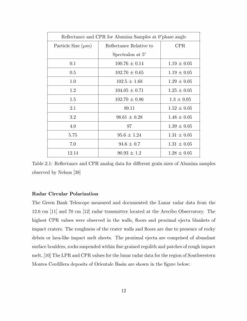
Analog Sample Polarization
In a study conducted by R. Nelson and B. Hapke, they observed the relative reflectance
and CPR values for various grain sizes of alumina samples. [37] A long arm gonio-
polarimeter was used by the author to acquire these measurements with the wavelength
of illuminating radiation being 0.633 µm. The CPR values of alumina grain sizes at zero
phase angle and the relative reflectance compared to standard reference Spectralon sample
at 5°are shown below with their measurement errors:
The polarimetric apparatus used by Nelson consisted of an off-axis analyzer setup
which is capable of measuring reflectance from 0.05°- 5°phase angle. The apparatus used
different orientations of linear polarizers and quarter wave plates to observe the polariza-
tion state of the propagating signal. The CPR measurements from Nelson’s paper shown
in Table 2.1, suggests that the highest values are observed for particle sizes that are within
a few wavelengths of the incident radiation. Higher reflectance values are observed for
particles sizes closer to the wavelength while low reflectance values are observed for sizes
much smaller to larger than the incident wavelength.
11
Reflectance and CPR for Alumina Samples at 0°phase angle
Particle Size (µm) Reflectance Relative to
Spectralon at 5°
CPR
0.1 100.76 ± 0.14 1.19 ± 0.05
0.5 102.70 ± 0.65 1.19 ± 0.05
1.0 102.5 ± 1.68 1.29 ± 0.05
1.2 104.05 ± 0.71 1.25 ± 0.05
1.5 102.70 ± 0.86 1.3 ± 0.05
2.1 99.11 1.52 ± 0.05
3.2 98.61 ± 0.28 1.48 ± 0.05
4.0 97 1.39 ± 0.05
5.75 95.6 ± 1.24 1.31 ± 0.05
7.0 94.6 ± 0.7 1.31 ± 0.05
12.14 90.93 ± 1.2 1.28 ± 0.05
Table 2.1: Reflectance and CPR analog data for different grain sizes of Alumina samples
observed by Nelson [38]
Radar Circular Polarization
The Green Bank Telescope measured and documented the Lunar radar data from the
12.6 cm [11] and 70 cm [12] radar transmitter located at the Arecibo Observatory. The
highest CPR values were observed in the walls, floors and proximal ejecta blankets of
impact craters. The roughness of the crater walls and floors are due to presence of rocky
debris or lava-like impact melt sheets. The proximal ejecta are comprised of abundant
surface boulders, rocks suspended within fine grained regolith and patches of rough impact
melt. [10] The LPR and CPR values for the lunar radar data for the region of Southwestern
Montes Cordillera deposits of Orientale Basin are shown in the figure below:
12
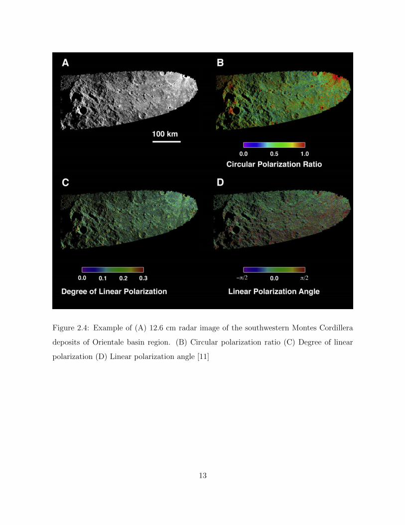
Figure 2.4: Example of (A) 12.6 cm radar image of the southwestern Montes Cordillera
deposits of Orientale basin region. (B) Circular polarization ratio (C) Degree of linear
polarization (D) Linear polarization angle [11]
13
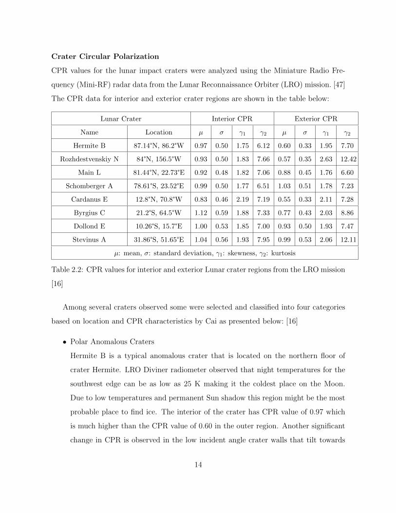
Crater Circular Polarization
CPR values for the lunar impact craters were analyzed using the Miniature Radio Fre-
quency (Mini-RF) radar data from the Lunar Reconnaissance Orbiter (LRO) mission. [47]
The CPR data for interior and exterior crater regions are shown in the table below:
Lunar Crater Interior CPR Exterior CPR
Name Location µ σ γ1 γ2 µ σ γ1 γ2
Hermite B 87.14°N, 86.2°W 0.97 0.50 1.75 6.12 0.60 0.33 1.95 7.70
Rozhdestvenskiy N 84°N, 156.5°W 0.93 0.50 1.83 7.66 0.57 0.35 2.63 12.42
Main L 81.44°N, 22.73°E 0.92 0.48 1.82 7.06 0.88 0.45 1.76 6.60
Schomberger A 78.61°S, 23.52°E 0.99 0.50 1.77 6.51 1.03 0.51 1.78 7.23
Cardanus E 12.8°N, 70.8°W 0.83 0.46 2.19 7.19 0.55 0.33 2.11 7.28
Byrgius C 21.2°S, 64.5°W 1.12 0.59 1.88 7.33 0.77 0.43 2.03 8.86
Dollond E 10.26°S, 15.7°E 1.00 0.53 1.85 7.00 0.93 0.50 1.93 7.47
Stevinus A 31.86°S, 51.65°E 1.04 0.56 1.93 7.95 0.99 0.53 2.06 12.11
µ: mean, σ: standard deviation, γ1: skewness, γ2: kurtosis
Table 2.2: CPR values for interior and exterior Lunar crater regions from the LRO mission
[16]
Among several craters observed some were selected and classified into four categories
based on location and CPR characteristics by Cai as presented below: [16]
• Polar Anomalous Craters
Hermite B is a typical anomalous crater that is located on the northern floor of
crater Hermite. LRO Diviner radiometer observed that night temperatures for the
southwest edge can be as low as 25 K making it the coldest place on the Moon.
Due to low temperatures and permanent Sun shadow this region might be the most
probable place to find ice. The interior of the crater has CPR value of 0.97 which
is much higher than the CPR value of 0.60 in the outer region. Another significant
change in CPR is observed in the low incident angle crater walls that tilt towards
14
the radar which corresponds to large SC and OC scatter resulting in a smaller CPR
value. [16]
• Non-Polar Anomalous Craters
Cardanus E is a bowl-shaped crater that is located close to the Southwest edge
of Oceanus Procellarum. The crater has varying thermal conditions due to which
water ice is not expected to stay stable within this region. This is reflected in the
CPR values (Interior CPR =0.83, Exterior CPR = 0.55) which are lower than the
polar anomalous crater regions. The large CPR differences in the interior to exterior
regions are due to the slope of the crater wall which varies from 20°to 30°. The radar
echoes for the crater that tilt towards the radar are twice as those for the entire
interior region while echoes from crater walls that tilt away are one-third as those
for interior region. [16]
• Polar Fresh Craters
Main L is a bowl-shaped fresh crater that is located in the North Polar Region with
most of its portions covered in permanent shadow except portions of the Northern
rim. The CPR values for the interior (CPR = 0.92) and exterior regions (CPR
= 0.88) are in close proximity to each other. The correlation between radar echo
strengths and local incidence angles are very strong where large incidence angles
have lower radar returns while smaller incidence angles have large radar returns and
higher CPR. [16]
• Non-polar Fresh Craters
Dollond E is a bowl-shaped crater located to the west of Mare Nectaris with sig-
nificantly high CPR values in both its interior (CPR = 1.0) and exterior (CPR =
0.93) regions. The crater has high elevation differences and the slope of crater wall
varies from 20°-35°. Due to these parameters we observe high CPR in comparison
to the other craters types. [16]
15
The presented crater polarization data suggests that the primary factor for elevated
CPRs in the interior regions of the anomalous craters were attributed to icy deposits
due to its correlations with Lunar Prospector neutron data and thermal conditions like
cold traps and permanent shadowing. The CPR values of the lunar surface depended on
various parameters such as, radar frequency, incidence angle, surface roughness, surface
slope, dielectric constant, size and shape of surface and sub-surface rocks and regolith
thickness. Theoretical simulations from the paper suggests that from all the parameters
that influenced polarization data, radar incidence angle was the most prominent factor
that influenced radar echo strength and CPR value. [17] While taking the slope of crater
wall into account the mean CPR of the interior region was much higher than the exterior
region for anomalous crater. For fresh craters the mean CPR for crater wall that tilted
towards the radar (small incidence angle) was smaller than that of the exterior region
which suggests that slope of the crater wall plays an important role in determining the
CPR value. In observation the polar anomalous craters had higher CPR values than
the non-polar regions indicating presence of water ice however newly formed craters also
possessed a higher CPR value due to the crater sloping and changes in incidence angles.
Hence we can say that high CPR parameter was not only a function of icy versus non-icy
regions but also depended on radar configuration and surface properties. [16]
16
2.3 Mueller Matrix
The polarization of light provides valuable information regarding the physical state of
an optical component. [25] In high precision polarimetry, it is important to calibrate the
instrumental polarization of the observing system with required accuracy. The charac-
terization of optical components can be achieved by measuring the Mueller matrices of
optical elements. A Mueller matrix is a 4 x 4 real valued matrix that characterizes the
optical properties of the sample by the interaction of polarized light in either reflection
or transmission configurations. [32]
The polarization state of an electromagnetic wave can be determined by measuring
the Stokes vector of the signal. The electromagnetic wave would have a different emerging
polarization when propagating through an optical element either by transmission reflection
or combination of both. The matrix method used to determine the output polarization
of an electromagnetic wave represented by a Stokes vector is called Mueller calculus. [43]
For an electromagnetic wave with initial polarization state Si propagating through an
optical component with M, Mueller matrix would have the output polarization state So
represented as Stokes vector [43]
So = MSi
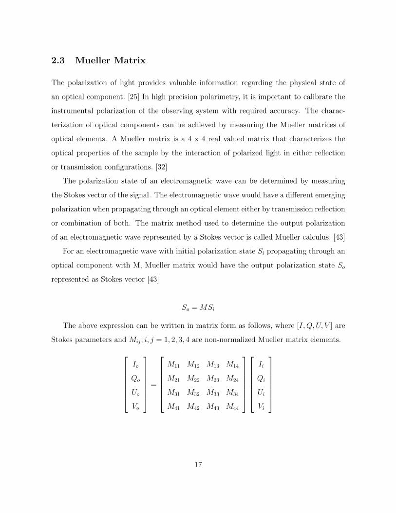
The above expression can be written in matrix form as follows, where [I,Q, U, V ] are
Stokes parameters and Mij; i, j = 1, 2, 3, 4 are non-normalized Mueller matrix elements.
Io
Qo
Uo
Vo
=
M11 M12 M13 M14
M21 M22 M23 M24
M31 M32 M33 M34
M41 M42 M43 M44
Ii
Qi
Ui
Vi
17

Figure 2.5: An electromagnetic wave interacting with (a) single and (b) multiple cascad-
ing optical systems with M, Mueller matrices.Ei and E0 indicates the input and output
polarization ellipse of the wave [32]
When an electromagnetic wave interacts with several optical systems in cascade as
shown in figure 3.1, the polarization ellipse or Stokes vector of the emerging wave can be
calculated as
Eo = Mn...M2M1Ei
The absolute Mueller matrix elements are calculated by normalizing the Mueller ma-
trix with its first element, mij = Mij/M11. The Normalized Mueller matrix are often used
when calculating the output Stokes parameter from the input polarization state. [20]
18
2.3.1 Examples of Mueller Matrices for Optical Components
The Mueller matrices for a variety of optical components used in this study are listed
below:
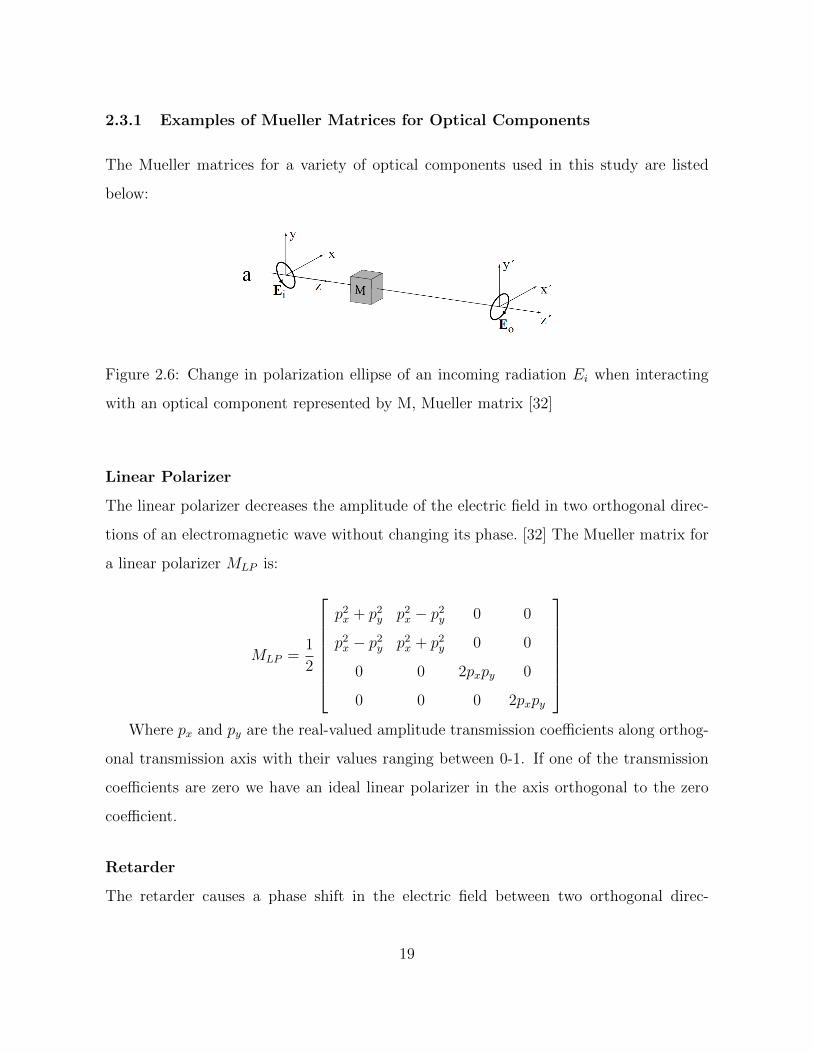
Figure 2.6: Change in polarization ellipse of an incoming radiation Ei when interacting
with an optical component represented by M, Mueller matrix [32]
Linear Polarizer
The linear polarizer decreases the amplitude of the electric field in two orthogonal direc-
tions of an electromagnetic wave without changing its phase. [32] The Mueller matrix for
a linear polarizer MLP is:
MLP =1
2
p2x + p2y p2x − p2y 0 0
p2x − p2y p2x + p2y 0 0
0 0 2pxpy 0
0 0 0 2pxpy
Where px and py are the real-valued amplitude transmission coefficients along orthog-
onal transmission axis with their values ranging between 0-1. If one of the transmission
coefficients are zero we have an ideal linear polarizer in the axis orthogonal to the zero
coefficient.
Retarder
The retarder causes a phase shift in the electric field between two orthogonal direc-
19
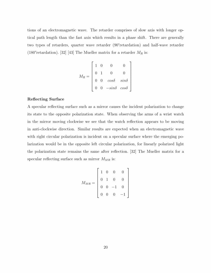
tions of an electromagnetic wave. The retarder comprises of slow axis with longer op-
tical path length than the fast axis which results in a phase shift. There are generally
two types of retarders, quarter wave retarder (90°retardation) and half-wave retarder
(180°retardation). [32] [43] The Mueller matrix for a retarder MR is:
MR =
1 0 0 0
0 1 0 0
0 0 cosδ sinδ
0 0 −sinδ cosδ
Reflecting Surface
A specular reflecting surface such as a mirror causes the incident polarization to change
its state to the opposite polarization state. When observing the arms of a wrist watch
in the mirror moving clockwise we see that the watch reflection appears to be moving
in anti-clockwise direction. Similar results are expected when an electromagnetic wave
with right circular polarization is incident on a specular surface where the emerging po-
larization would be in the opposite left circular polarization, for linearly polarized light
the polarization state remains the same after reflection. [32] The Mueller matrix for a
specular reflecting surface such as mirror MMR is:
MMR =
1 0 0 0
0 1 0 0
0 0 −1 0
0 0 0 −1
20

No Sample
The Mueller matrix of an electromagnetic wave propagating without any reflection or
interference is an identity matrix often represented as m′ij = δiji0 where δij is the Kro-
necker delta function. The no sample measurement configuration is used in the instru-
ment calibration procedure where the polarimeter is operated with straight-through signal
propagation. [20] The Mueller matrix for a no sample setup MC is:
MC =
1 0 0 0
0 1 0 0
0 0 1 0
0 0 0 1
21
2.4 Opposition Effects
The surge in brightness of a particulate medium observed near zero phase angle is called
the opposition effect. [23] The opposition effect was first noted by Seeliger [21] on Saturn’s
rings and has since been observed on a variety of bodies including the Moon, Mars,
asteroids, planetary satellites and terrestrial materials.
When observing a particulate medium at the same angle as the incidence angle of the
light source there is a surge in brightness that can be attributed to the opposition effect.
These effects are also observed around terrestrial regions such as forests, grass fields and
deserts when the sun is directly overhead the observer. [22]
The existence of the opposition surge were first described by Tom Gehrels during his
study of the reflected light from the asteroid. [18] Suggestions such that the coherent
backscatter causes the opposition effects for the solar system bodies at visual wavelength
and coherent effect might also account for the negative branch of polarization for planetary
bodies are plausible. [35] However because the solar system objects are illuminated with
natural sunlight that is unpolarized, the astronomical opposition effects have ambiguous
interpretations. [24]
22
2.4.1 Shadow Hiding Opposition Effect
The opposition effect causing a sharp surge in brightness of an astronomical object ob-
served near zero phase angle has generally been explained by Shadow hiding (SHOE).
SHOE results when particles in a planetary regolith cast shadows on adjacent particles;
those shadows are visible at larger observation angles but as we get progressively closer to
the incidence angle, the shadows are hidden beneath the particles that cast them causing
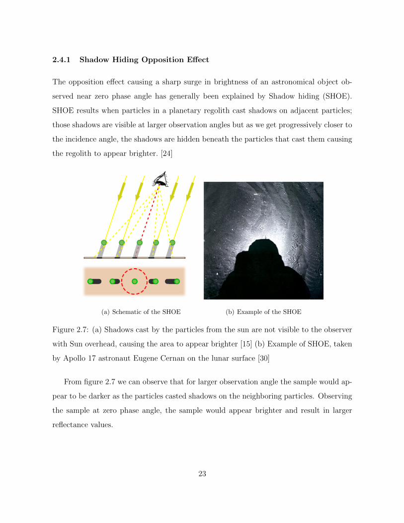
the regolith to appear brighter. [24]
(a) Schematic of the SHOE (b) Example of the SHOE
Figure 2.7: (a) Shadows cast by the particles from the sun are not visible to the observer
with Sun overhead, causing the area to appear brighter [15] (b) Example of SHOE, taken
by Apollo 17 astronaut Eugene Cernan on the lunar surface [30]
From figure 2.7 we can observe that for larger observation angle the sample would ap-
pear to be darker as the particles casted shadows on the neighboring particles. Observing
the sample at zero phase angle, the sample would appear brighter and result in larger
reflectance values.
23
2.4.2 Coherent Backscattering Effect
The Coherent Backscattering Opposition effect (CBOE) also known as weak photon local-
ization through time reversal symmetry [3] is based on the fact that portions of wave fronts
that are multiple scattered within a nonuniform medium follow the same path, but those
in opposite directions combine constructively at zero phase angle to produce a brightness
peak. The CBOE is most prominent when the particles are of the order of wavelength
in size and have high single-scattering albedos, due to constructive combination of the
amplitudes of the emerging waves. The coherent backscattering effect was responsible for
most of the planetary opposition surges observed in the solar system. [23] [24]
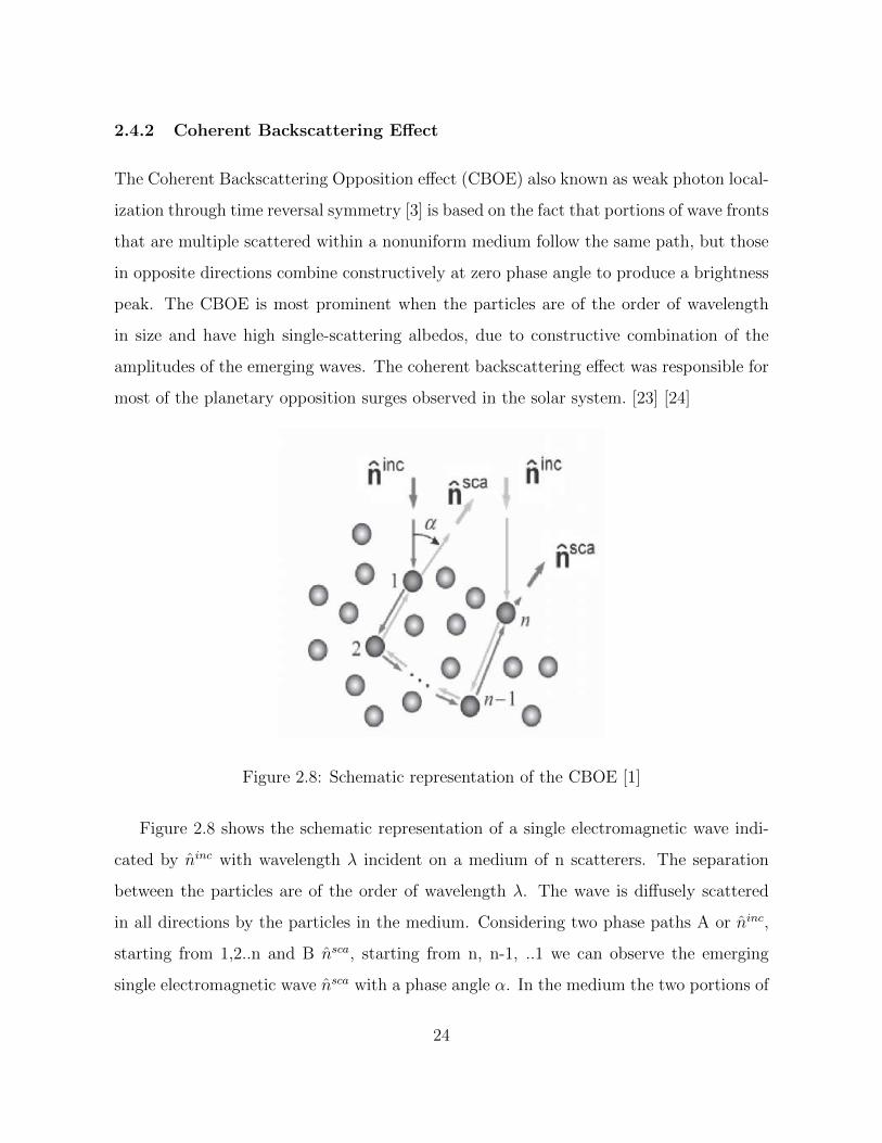
Figure 2.8: Schematic representation of the CBOE [1]
Figure 2.8 shows the schematic representation of a single electromagnetic wave indi-
cated by ninc with wavelength λ incident on a medium of n scatterers. The separation
between the particles are of the order of wavelength λ. The wave is diffusely scattered
in all directions by the particles in the medium. Considering two phase paths A or ninc,
starting from 1,2..n and B nsca, starting from n, n-1, ..1 we can observe the emerging
single electromagnetic wave nsca with a phase angle α. In the medium the two portions of
24
the wave A and B traverse exactly the same path between 1 and n, but in opposite direc-
tions with numerous scatterings between particles along the path. The relative difference
in phase between the parts of the wave that traverse along the same plane in opposite
directions can be shown in equation below, with X being the distance between particles
1 and n.
∆φ = (ninc + nsca)X
At exact zero phase angle the phase difference ∆φ between the two emerging waves
is zero which leads to the two parts of the wave interacting constructively. If the ampli-
tudes of the electric fields associated with the parts of the wave are E, then for random
phase orientation we observe their combines intensities as 2|E|2. However in the exact
backscattering direction the combined intensities are 4|E|2 for near zero phase angle. Due
to high intensity coherence for near zero phase angles compared to larger phase angles
the reflectance and CPR values are higher for CBOE. [23]
2.4.3 Properties of SHOE and CBOE
1. The Shadow Hiding Opposition Effect results from singly scattered light such that
the height of the peak relative to the continuum brightness decreases as the re-
flectance of the medium increases. As CBOE depends on multiple scattered light
the peak to continuum ratio increases as the reflectance increases.
2. The angular width of the SHOE peak depends on the scatterer mean separation and
size distribution. While the CBOE angular width depends linearly on wavelength.
The full width of the CBOE peak at half maximum (FWHM) can be calculated as:
∆gFWHM =0.72λ
2πD
Where, λ is the wavelength of the incident radiation, D is the diffusion length.
Nelson [37] observed very weak correlation between the theoretical predictions and
25
measured angular width of the phase curves for highly reflective alumina samples.
The variation in particle size distribution for any given size were larger than the
theoretical estimates used in the study.
3. Single reflections tend to preserve the direction of polarization for linearly polarized
incident light while multiple scatterings tend to randomize them. Thus the SHOE
peak is largely polarized in the same sense as the incident radiation while the light
scattered in the opposite sense has no opposition surge.
4. For circularly polarized incident radiation the single reflecting events tends to change
the polarization to the opposite sense while multiple scatterings tends to randomize
the polarization. This results in SHOE peak having strong circular polarization in
the opposite sense while CBOE contains both senses of polarization. [23]
26
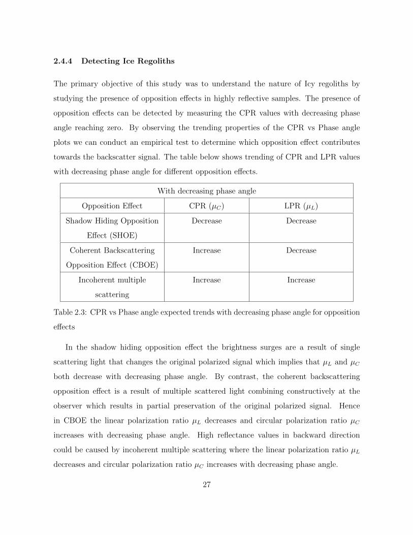
2.4.4 Detecting Ice Regoliths
The primary objective of this study was to understand the nature of Icy regoliths by
studying the presence of opposition effects in highly reflective samples. The presence of
opposition effects can be detected by measuring the CPR values with decreasing phase
angle reaching zero. By observing the trending properties of the CPR vs Phase angle
plots we can conduct an empirical test to determine which opposition effect contributes
towards the backscatter signal. The table below shows trending of CPR and LPR values
with decreasing phase angle for different opposition effects.
With decreasing phase angle
Opposition Effect CPR (µC) LPR (µL)
Shadow Hiding Opposition
Effect (SHOE)
Decrease Decrease
Coherent Backscattering
Opposition Effect (CBOE)
Increase Decrease
Incoherent multiple
scattering
Increase Increase
Table 2.3: CPR vs Phase angle expected trends with decreasing phase angle for opposition
effects
In the shadow hiding opposition effect the brightness surges are a result of single
scattering light that changes the original polarized signal which implies that µL and µC
both decrease with decreasing phase angle. By contrast, the coherent backscattering
opposition effect is a result of multiple scattered light combining constructively at the
observer which results in partial preservation of the original polarized signal. Hence
in CBOE the linear polarization ratio µL decreases and circular polarization ratio µC
increases with decreasing phase angle. High reflectance values in backward direction
could be caused by incoherent multiple scattering where the linear polarization ratio µL
decreases and circular polarization ratio µC increases with decreasing phase angle.
27

Various undertaken studies have shown that CBOE are the dominating cause of op-
position surge when the particles are in the size vicinity of the wavelength. For freshly
prepared small-grained spherical water-ice material, the coherent backscattering effect is
the dominating opposition effect but its contribution decreases when particles become
more irregularly shaped and the bulk porosity increases. [28]
28
3 Techniques Deployed for Measuring Data
3.1 Measuring Stokes Parameters
3.1.1 Rotating Quarter Wave Plate Technique
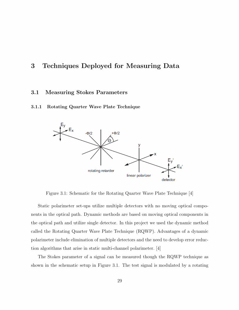
Figure 3.1: Schematic for the Rotating Quarter Wave Plate Technique [4]
Static polarimeter set-ups utilize multiple detectors with no moving optical compo-
nents in the optical path. Dynamic methods are based on moving optical components in
the optical path and utilize single detector. In this project we used the dynamic method
called the Rotating Quarter Wave Plate Technique (RQWP). Advantages of a dynamic
polarimeter include elimination of multiple detectors and the need to develop error reduc-
tion algorithms that arise in static multi-channel polarimeter. [4]
The Stokes parameter of a signal can be measured though the RQWP technique as
shown in the schematic setup in Figure 3.1. The test signal is modulated by a rotating
29
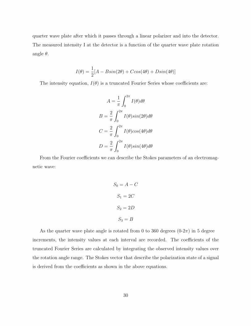
quarter wave plate after which it passes through a linear polarizer and into the detector.
The measured intensity I at the detector is a function of the quarter wave plate rotation
angle θ.
I(θ) =1
2[A−Bsin(2θ) + Ccos(4θ) +Dsin(4θ)]
The intensity equation, I(θ) is a truncated Fourier Series whose coefficients are:
A =1
π
∫ 2π
0
I(θ)dθ
B =2
π
∫ 2π
0
I(θ)sin(2θ)dθ
C =2
π
∫ 2π
0
I(θ)cos(4θ)dθ
D =2
π
∫ 2π
0
I(θ)sin(4θ)dθ
From the Fourier coefficients we can describe the Stokes parameters of an electromag-
netic wave:
S0 = A− C
S1 = 2C
S2 = 2D
S3 = B
As the quarter wave plate angle is rotated from 0 to 360 degrees (0-2π) in 5 degree
increments, the intensity values at each interval are recorded. The coefficients of the
truncated Fourier Series are calculated by integrating the observed intensity values over
the rotation angle range. The Stokes vector that describe the polarization state of a signal
is derived from the coefficients as shown in the above equations.
30
3.2 Measuring Mueller Matrix
The polarization state of an electromagnetic wave can be determined by measuring the
Stokes vector of the signal. The Stokes vector has four components that represent its total
intensity and polarization state. The signal propagating through an optical medium can
undergo polarization change that alters the Stokes parameters of the signal propagating
outward from the medium. A circularly polarized signal can alter its polarization state to
elliptically polarized light while propagating through an optical medium. We can correct
for these polarization alterations by measuring the Mueller matrices of the optical medium
and determining its impact on the Stokes parameters. [20]
3.2.1 Dual Rotating Quarter Wave Plate Technique
The Mueller matrix of an optical component is measured using the dual rotating quarter
wave plate technique that determines its polarization properties and its impact on the
propagating signal. The errors in retardance of the quarter wave plate, imperfect retar-
dation increment and misalignment in the polarizing components can be corrected using
error analysis. [4] [20]
The Dual rotating quarter wave plate technique measures a chopped signal that is
modulated by rotating the polarizing optical elements. The signal is Fourier analyzed after
passing through linear polarizers and dual rotating retarders to determine the Mueller
matrix elements. As shown in figure the two fixed linear polarizers and rotating quarter
wave plates are aligned with respect to their transmission axes and fast axes. The second
retarder is rotated at five times the rate the first retarder is rotated which generates twelve
harmonic frequencies in the Fourier Spectrum of the modulated intensity. [20]
31
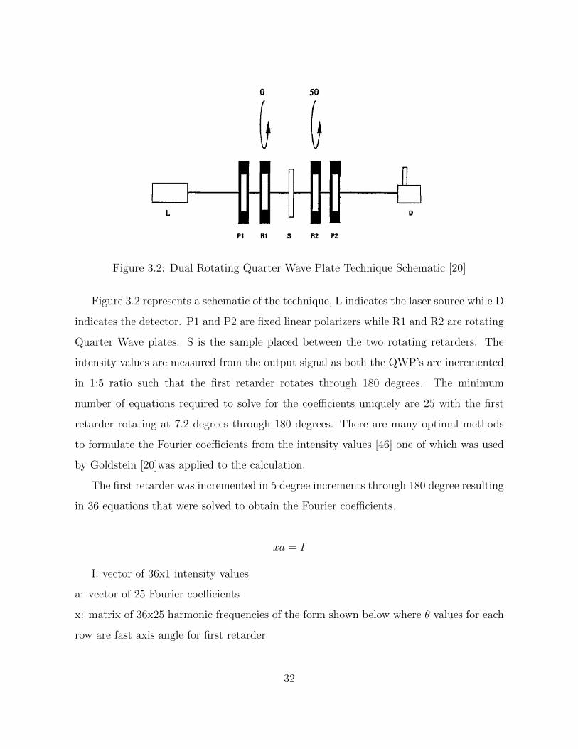
Figure 3.2: Dual Rotating Quarter Wave Plate Technique Schematic [20]
Figure 3.2 represents a schematic of the technique, L indicates the laser source while D
indicates the detector. P1 and P2 are fixed linear polarizers while R1 and R2 are rotating
Quarter Wave plates. S is the sample placed between the two rotating retarders. The
intensity values are measured from the output signal as both the QWP’s are incremented
in 1:5 ratio such that the first retarder rotates through 180 degrees. The minimum
number of equations required to solve for the coefficients uniquely are 25 with the first
retarder rotating at 7.2 degrees through 180 degrees. There are many optimal methods
to formulate the Fourier coefficients from the intensity values [46] one of which was used
by Goldstein [20]was applied to the calculation.
The first retarder was incremented in 5 degree increments through 180 degree resulting
in 36 equations that were solved to obtain the Fourier coefficients.
xa = I
I: vector of 36x1 intensity values
a: vector of 25 Fourier coefficients
x: matrix of 36x25 harmonic frequencies of the form shown below where θ values for each
row are fast axis angle for first retarder
32
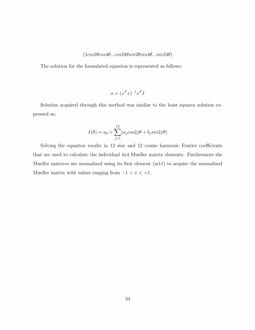
(1cos2θcos4θ...cos24θsin2θsin4θ...sin24θ)
The solution for the formulated equation is represented as follows;
a = (xTx)−1xT I
Solution acquired through this method was similar to the least squares solution ex-
pressed as;
I(θ) = a0 +12∑j=1
(ajcos2jθ + bjsin2jθ)
Solving the equation results in 12 sine and 12 cosine harmonic Fourier coefficients
that are used to calculate the individual 4x4 Mueller matrix elements. Furthermore the
Mueller matrices are normalized using its first element (m11) to acquire the normalized
Mueller matrix with values ranging from −1 < x < +1.
33
4 Instrumentation and Data Acquisition Procedures
4.1 Measurement Procedure
In this experiment the samples were illuminated with 15-20mW power Nd:YAG (neodymium-
doped yttrium aluminum garnet) laser at 1064nm or 1.064µm wavelength. The laser signal
was generated from a multi-channel fiber coupled laser source with four available incident
wavelengths. The schematic for the polarimeter assembly is shown in Figure 4.1, the
dimensions for the assembly are listed in Appendix A. The incident signal generated from
the laser source is fed through a fiber cable and attached to the caddy platform of the
goniometric instrument after which it passes through a collimator and linear polarizer.
The linearly polarized signal is chopped at a frequency of 250 Hz by using an optical
chopper. Beam divergence effects of the incident radiation were eliminated by placing a
focusing lens after the signal was chopped.
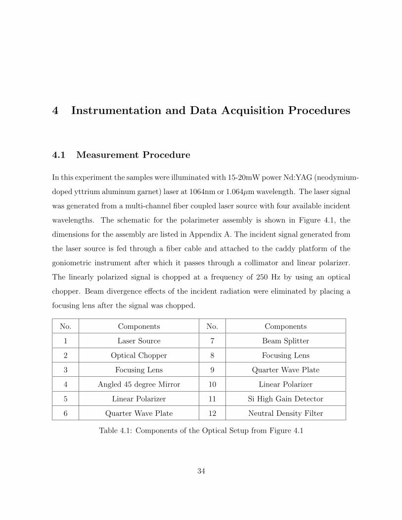
No. Components No. Components
1 Laser Source 7 Beam Splitter
2 Optical Chopper 8 Focusing Lens
3 Focusing Lens 9 Quarter Wave Plate
4 Angled 45 degree Mirror 10 Linear Polarizer
5 Linear Polarizer 11 Si High Gain Detector
6 Quarter Wave Plate 12 Neutral Density Filter
Table 4.1: Components of the Optical Setup from Figure 4.1
34
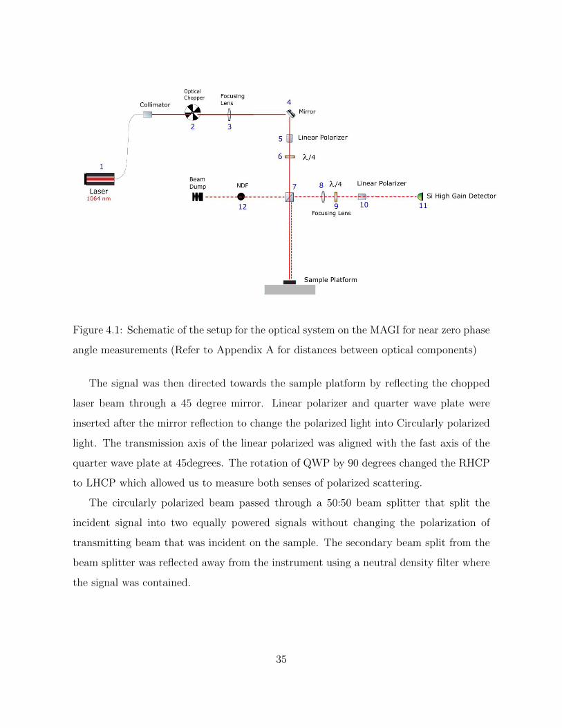
Figure 4.1: Schematic of the setup for the optical system on the MAGI for near zero phase
angle measurements (Refer to Appendix A for distances between optical components)
The signal was then directed towards the sample platform by reflecting the chopped
laser beam through a 45 degree mirror. Linear polarizer and quarter wave plate were
inserted after the mirror reflection to change the polarized light into Circularly polarized
light. The transmission axis of the linear polarized was aligned with the fast axis of the
quarter wave plate at 45degrees. The rotation of QWP by 90 degrees changed the RHCP
to LHCP which allowed us to measure both senses of polarized scattering.
The circularly polarized beam passed through a 50:50 beam splitter that split the
incident signal into two equally powered signals without changing the polarization of
transmitting beam that was incident on the sample. The secondary beam split from the
beam splitter was reflected away from the instrument using a neutral density filter where
the signal was contained.
35
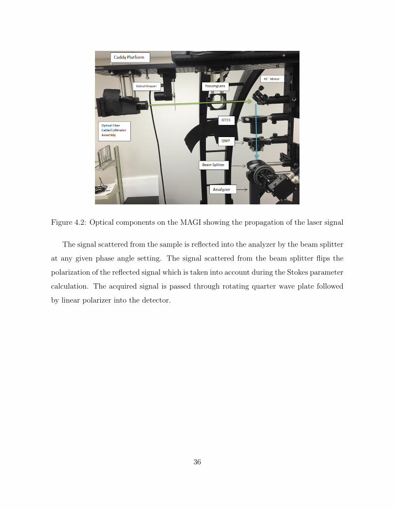
Figure 4.2: Optical components on the MAGI showing the propagation of the laser signal
The signal scattered from the sample is reflected into the analyzer by the beam splitter
at any given phase angle setting. The signal scattered from the beam splitter flips the
polarization of the reflected signal which is taken into account during the Stokes parameter
calculation. The acquired signal is passed through rotating quarter wave plate followed
by linear polarizer into the detector.
36
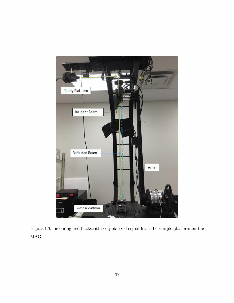
Figure 4.3: Incoming and backscattered polarized signal from the sample platform on the
MAGI
37
4.2 Multi-Axis Goniometric Instrument
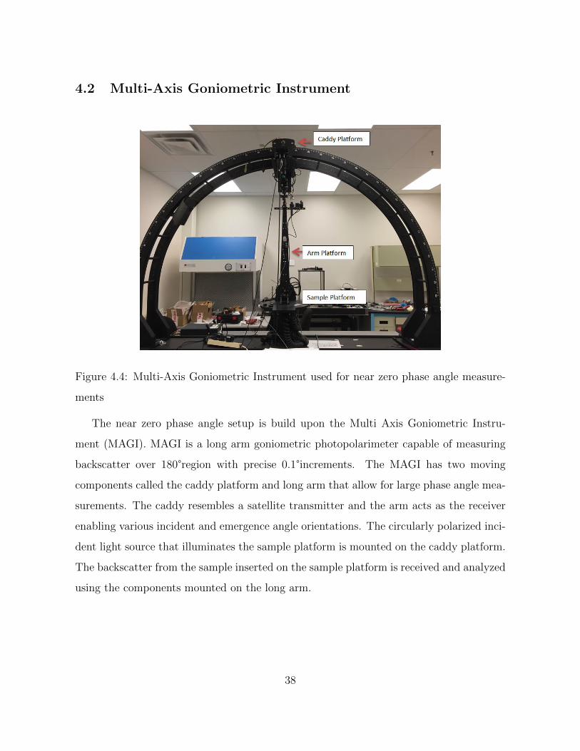
Figure 4.4: Multi-Axis Goniometric Instrument used for near zero phase angle measure-
ments
The near zero phase angle setup is build upon the Multi Axis Goniometric Instru-
ment (MAGI). MAGI is a long arm goniometric photopolarimeter capable of measuring
backscatter over 180°region with precise 0.1°increments. The MAGI has two moving
components called the caddy platform and long arm that allow for large phase angle mea-
surements. The caddy resembles a satellite transmitter and the arm acts as the receiver
enabling various incident and emergence angle orientations. The circularly polarized inci-
dent light source that illuminates the sample platform is mounted on the caddy platform.
The backscatter from the sample inserted on the sample platform is received and analyzed
using the components mounted on the long arm.
38
Near zero phase angle measurements were recorded from 0-5 degree phase angle in
0.1 degree increments. The long arm is kept in 0 degree emergence angle position as the
caddy platform moves from 0-5 degree incidence angle. Similar results are expected when
keeping the caddy platform stationary and moving the long arm platform. The heavy
weight of the analyzer component mounted on the long arm significantly limits the arm’s
movement.
4.2.1 Caddy Platform
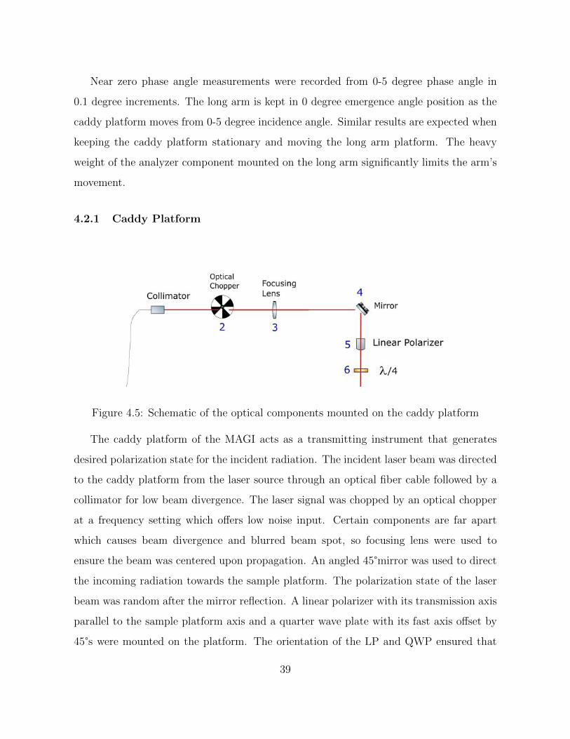
Figure 4.5: Schematic of the optical components mounted on the caddy platform
The caddy platform of the MAGI acts as a transmitting instrument that generates
desired polarization state for the incident radiation. The incident laser beam was directed
to the caddy platform from the laser source through an optical fiber cable followed by a
collimator for low beam divergence. The laser signal was chopped by an optical chopper
at a frequency setting which offers low noise input. Certain components are far apart
which causes beam divergence and blurred beam spot, so focusing lens were used to
ensure the beam was centered upon propagation. An angled 45°mirror was used to direct
the incoming radiation towards the sample platform. The polarization state of the laser
beam was random after the mirror reflection. A linear polarizer with its transmission axis
parallel to the sample platform axis and a quarter wave plate with its fast axis offset by
45°s were mounted on the platform. The orientation of the LP and QWP ensured that
39
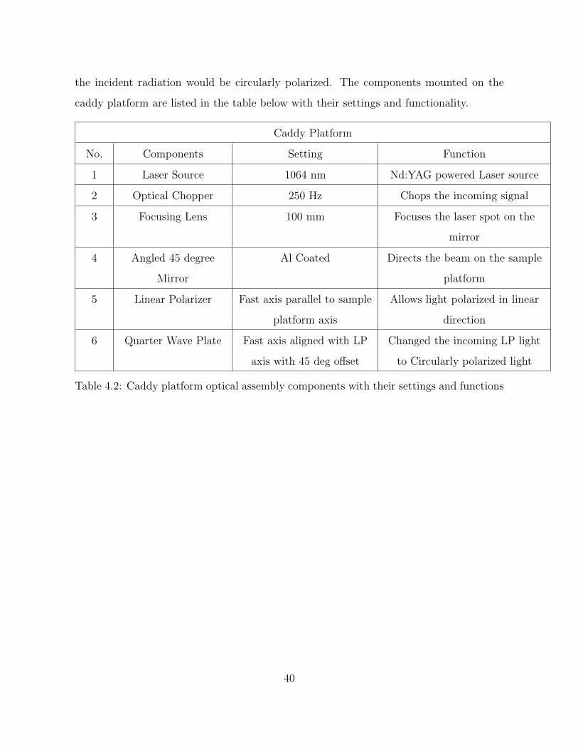
the incident radiation would be circularly polarized. The components mounted on the
caddy platform are listed in the table below with their settings and functionality.
Caddy Platform
No. Components Setting Function
1 Laser Source 1064 nm Nd:YAG powered Laser source
2 Optical Chopper 250 Hz Chops the incoming signal
3 Focusing Lens 100 mm Focuses the laser spot on the
mirror
4 Angled 45 degree
Mirror
Al Coated Directs the beam on the sample
platform
5 Linear Polarizer Fast axis parallel to sample
platform axis
Allows light polarized in linear
direction
6 Quarter Wave Plate Fast axis aligned with LP
axis with 45 deg offset
Changed the incoming LP light
to Circularly polarized light
Table 4.2: Caddy platform optical assembly components with their settings and functions
40
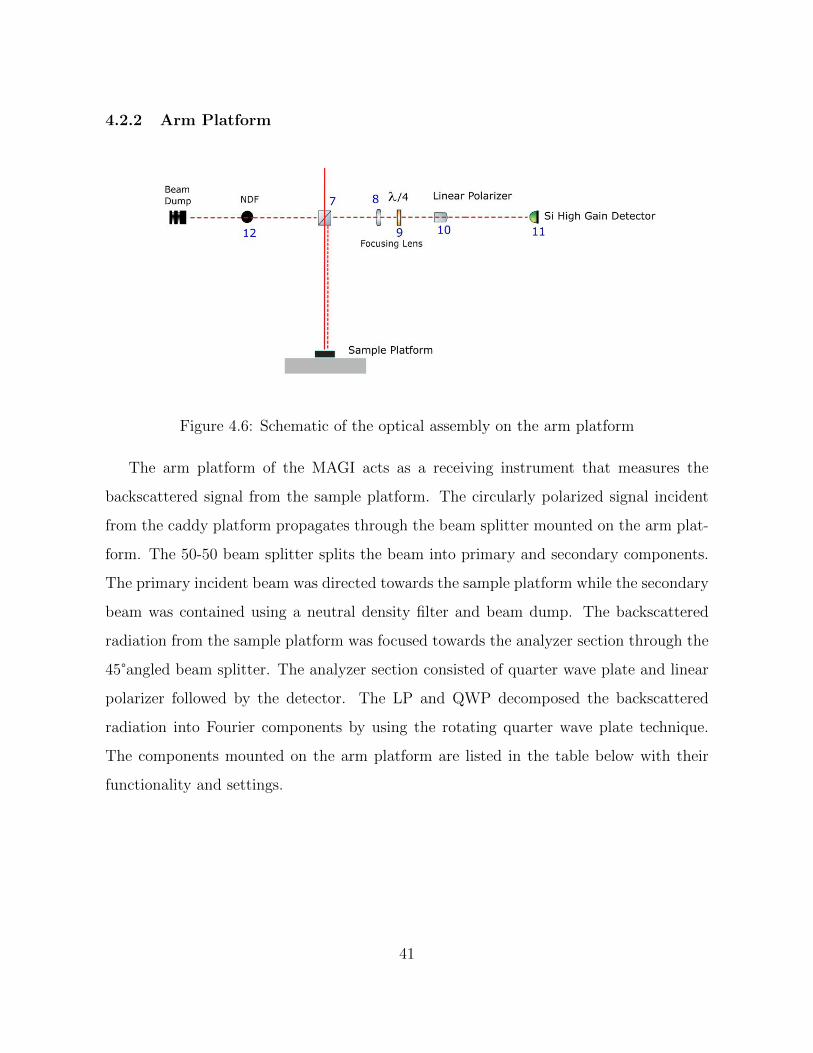
4.2.2 Arm Platform
Figure 4.6: Schematic of the optical assembly on the arm platform
The arm platform of the MAGI acts as a receiving instrument that measures the
backscattered signal from the sample platform. The circularly polarized signal incident
from the caddy platform propagates through the beam splitter mounted on the arm plat-
form. The 50-50 beam splitter splits the beam into primary and secondary components.
The primary incident beam was directed towards the sample platform while the secondary
beam was contained using a neutral density filter and beam dump. The backscattered
radiation from the sample platform was focused towards the analyzer section through the
45°angled beam splitter. The analyzer section consisted of quarter wave plate and linear
polarizer followed by the detector. The LP and QWP decomposed the backscattered
radiation into Fourier components by using the rotating quarter wave plate technique.
The components mounted on the arm platform are listed in the table below with their
functionality and settings.
41
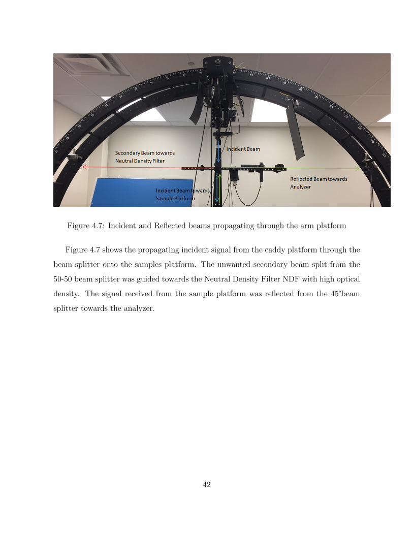
Figure 4.7: Incident and Reflected beams propagating through the arm platform
Figure 4.7 shows the propagating incident signal from the caddy platform through the
beam splitter onto the samples platform. The unwanted secondary beam split from the
50-50 beam splitter was guided towards the Neutral Density Filter NDF with high optical
density. The signal received from the sample platform was reflected from the 45°beam
splitter towards the analyzer.
42
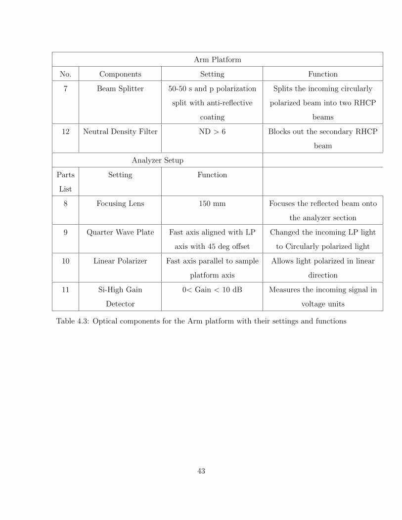
Arm Platform
No. Components Setting Function
7 Beam Splitter 50-50 s and p polarization
split with anti-reflective
coating
Splits the incoming circularly
polarized beam into two RHCP
beams
12 Neutral Density Filter ND > 6 Blocks out the secondary RHCP
beam
Analyzer Setup
Parts
List
Setting Function
8 Focusing Lens 150 mm Focuses the reflected beam onto
the analyzer section
9 Quarter Wave Plate Fast axis aligned with LP
axis with 45 deg offset
Changed the incoming LP light
to Circularly polarized light
10 Linear Polarizer Fast axis parallel to sample
platform axis
Allows light polarized in linear
direction
11 Si-High Gain
Detector
0< Gain < 10 dB Measures the incoming signal in
voltage units
Table 4.3: Optical components for the Arm platform with their settings and functions
43
4.3 Data Acquisition Setup
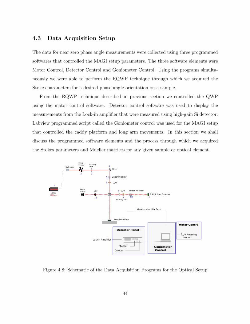
The data for near zero phase angle measurements were collected using three programmed
softwares that controlled the MAGI setup parameters. The three software elements were
Motor Control, Detector Control and Goniometer Control. Using the programs simulta-
neously we were able to perform the RQWP technique through which we acquired the
Stokes parameters for a desired phase angle orientation on a sample.
From the RQWP technique described in previous section we controlled the QWP
using the motor control software. Detector control software was used to display the
measurements from the Lock-in amplifier that were measured using high-gain Si detector.
Labview programmed script called the Goniometer control was used for the MAGI setup
that controlled the caddy platform and long arm movements. In this section we shall
discuss the programmed software elements and the process through which we acquired
the Stokes parameters and Mueller matrices for any given sample or optical element.
Figure 4.8: Schematic of the Data Acquisition Programs for the Optical Setup
44
4.3.1 Motor Control
(a) MotorControl (b) Rotation Stage
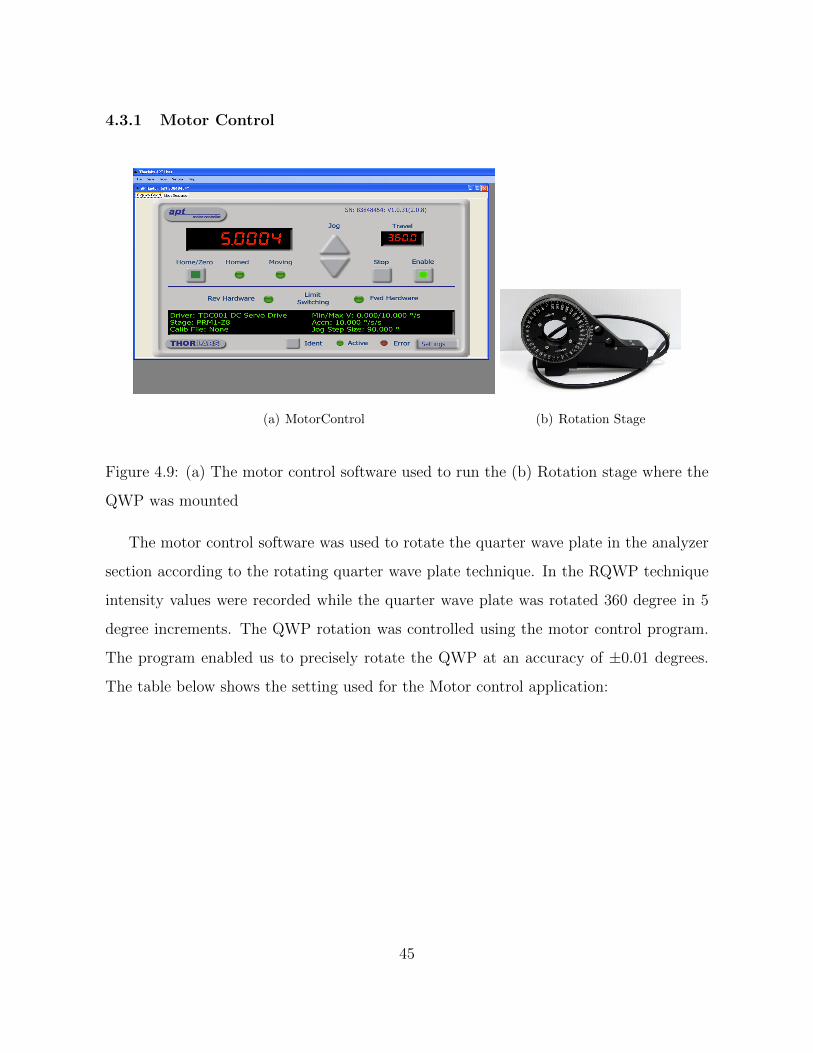
Figure 4.9: (a) The motor control software used to run the (b) Rotation stage where the
QWP was mounted
The motor control software was used to rotate the quarter wave plate in the analyzer
section according to the rotating quarter wave plate technique. In the RQWP technique
intensity values were recorded while the quarter wave plate was rotated 360 degree in 5
degree increments. The QWP rotation was controlled using the motor control program.
The program enabled us to precisely rotate the QWP at an accuracy of ±0.01 degrees.
The table below shows the setting used for the Motor control application:
45
Motor Control
Button Setting Function
Jog Step Size 5 degrees Increments the rotation stage
clockwise (Up) or
counter-clockwise (Down)
Acceleration 10 degrees/sec Speed at which the rotation
stage moves
Travel 360 degrees Overall rotation distance covered
by the rotation stage
Table 4.4: Motor Control Software settings used for operating the rotation stage
4.3.2 Detector Control
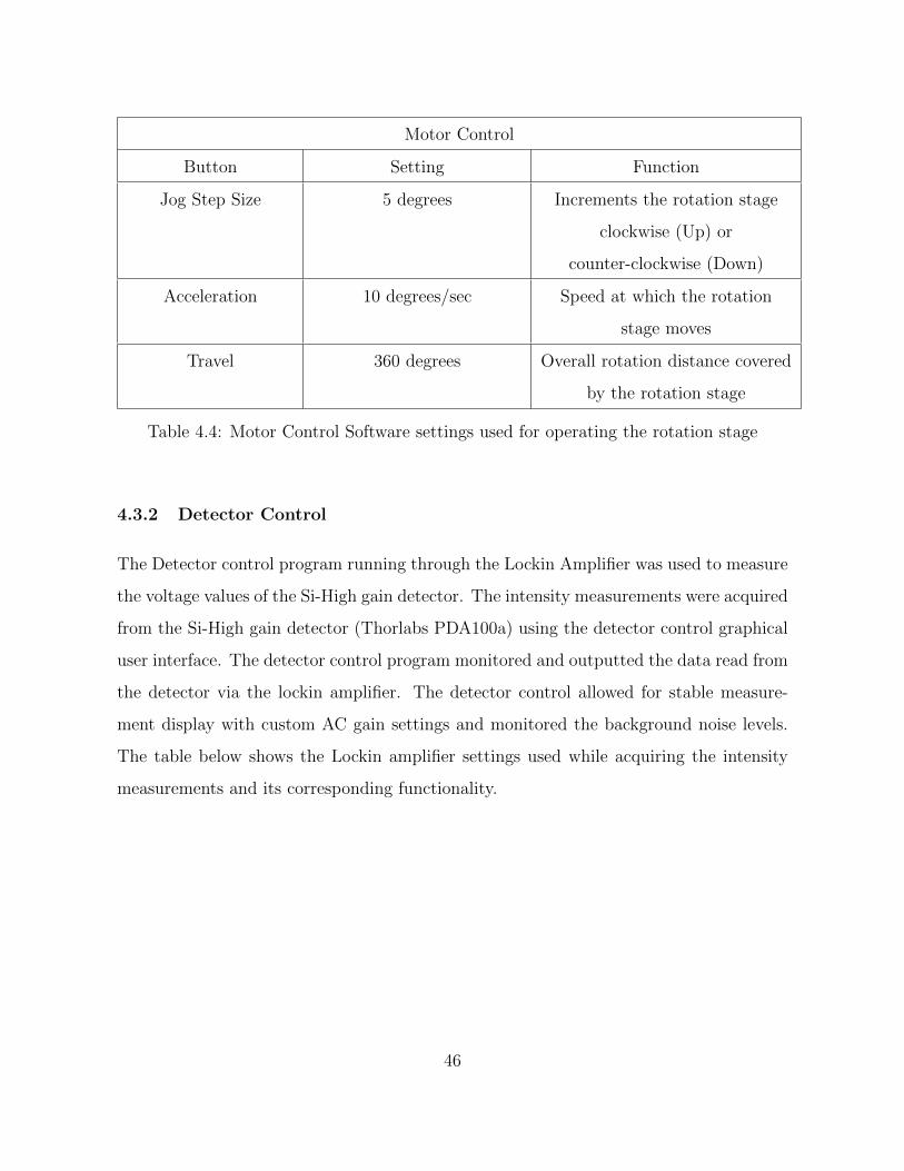
The Detector control program running through the Lockin Amplifier was used to measure
the voltage values of the Si-High gain detector. The intensity measurements were acquired
from the Si-High gain detector (Thorlabs PDA100a) using the detector control graphical
user interface. The detector control program monitored and outputted the data read from
the detector via the lockin amplifier. The detector control allowed for stable measure-
ment display with custom AC gain settings and monitored the background noise levels.
The table below shows the Lockin amplifier settings used while acquiring the intensity
measurements and its corresponding functionality.
46
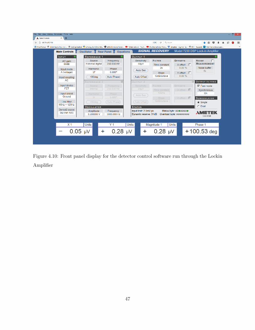
Figure 4.10: Front panel display for the detector control software run through the Lockin
Amplifier
47
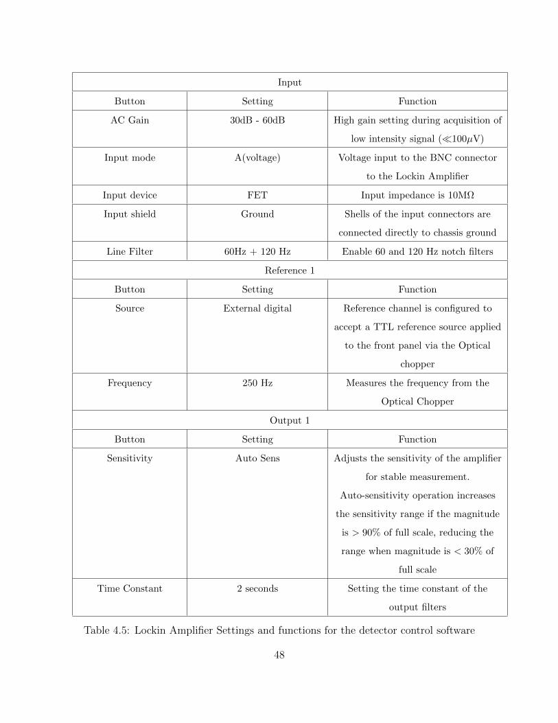
Input
Button Setting Function
AC Gain 30dB - 60dB High gain setting during acquisition of
low intensity signal (100µV)
Input mode A(voltage) Voltage input to the BNC connector
to the Lockin Amplifier
Input device FET Input impedance is 10MΩ
Input shield Ground Shells of the input connectors are
connected directly to chassis ground
Line Filter 60Hz + 120 Hz Enable 60 and 120 Hz notch filters
Reference 1
Button Setting Function
Source External digital Reference channel is configured to
accept a TTL reference source applied
to the front panel via the Optical
chopper
Frequency 250 Hz Measures the frequency from the
Optical Chopper
Output 1
Button Setting Function
Sensitivity Auto Sens Adjusts the sensitivity of the amplifier
for stable measurement.
Auto-sensitivity operation increases
the sensitivity range if the magnitude
is > 90% of full scale, reducing the
range when magnitude is < 30% of
full scale
Time Constant 2 seconds Setting the time constant of the
output filters
Table 4.5: Lockin Amplifier Settings and functions for the detector control software
48
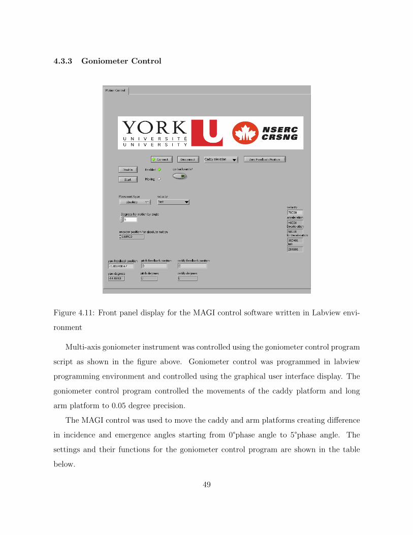
4.3.3 Goniometer Control
Figure 4.11: Front panel display for the MAGI control software written in Labview envi-
ronment
Multi-axis goniometer instrument was controlled using the goniometer control program
script as shown in the figure above. Goniometer control was programmed in labview
programming environment and controlled using the graphical user interface display. The
goniometer control program controlled the movements of the caddy platform and long
arm platform to 0.05 degree precision.
The MAGI control was used to move the caddy and arm platforms creating difference
in incidence and emergence angles starting from 0°phase angle to 5°phase angle. The
settings and their functions for the goniometer control program are shown in the table
below.
49
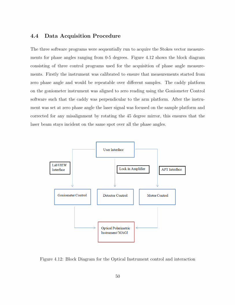
4.4 Data Acquisition Procedure
The three software programs were sequentially run to acquire the Stokes vector measure-
ments for phase angles ranging from 0-5 degrees. Figure 4.12 shows the block diagram
consisting of three control programs used for the acquisition of phase angle measure-
ments. Firstly the instrument was calibrated to ensure that measurements started from
zero phase angle and would be repeatable over different samples. The caddy platform
on the goniometer instrument was aligned to zero reading using the Goniometer Control
software such that the caddy was perpendicular to the arm platform. After the instru-
ment was set at zero phase angle the laser signal was focused on the sample platform and
corrected for any misalignment by rotating the 45 degree mirror, this ensures that the
laser beam stays incident on the same spot over all the phase angles.
Figure 4.12: Block Diagram for the Optical Instrument control and interaction
50
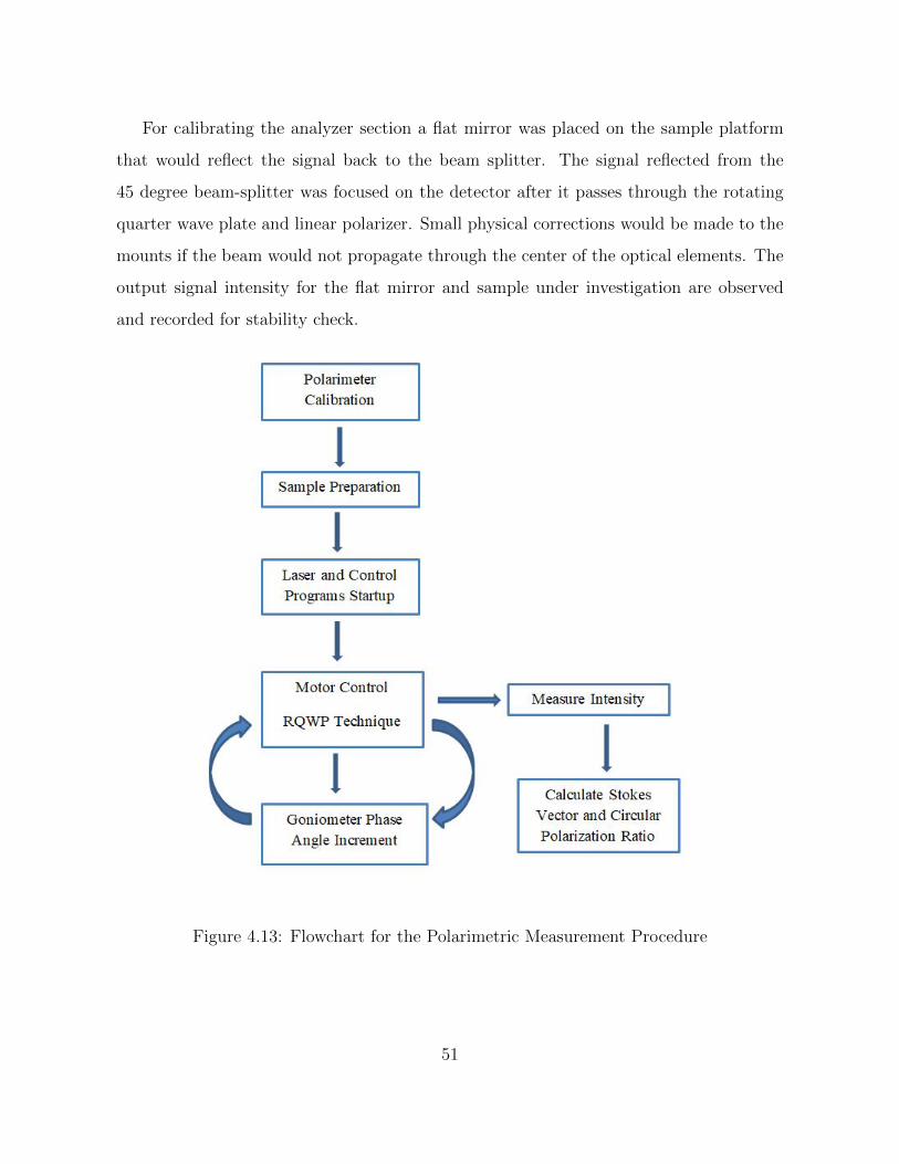
For calibrating the analyzer section a flat mirror was placed on the sample platform
that would reflect the signal back to the beam splitter. The signal reflected from the
45 degree beam-splitter was focused on the detector after it passes through the rotating
quarter wave plate and linear polarizer. Small physical corrections would be made to the
mounts if the beam would not propagate through the center of the optical elements. The
output signal intensity for the flat mirror and sample under investigation are observed
and recorded for stability check.
Figure 4.13: Flowchart for the Polarimetric Measurement Procedure
51
After calibrating the instrument and setting the caddy platform at zero phase an-
gle the measurements are recorded by the control programs. Figure 4.13 shows a high-
level flowchart describing the data acquisition procedure. Signal intensities are acquired
through the lock-in amplifier by rotating the QWP over 360 degrees using the motor con-
trol program for zero phase angle. The signal intensities over 360 degrees of QWP rotation
in 5 degree increments are passed through Fourier transforms to compute the Stokes pa-
rameters and CPR for the backscattered signal at zero phase angle. As the CPR for zero
phase angle was acquired the caddy platform was moved in increments of 0.1 degree over
range of 5 degrees using the goniometer control program. The Stokes parameters and
CPR values are computed for backscattered signal of each phase angle by performing the
rotating QWP method and incrementing the caddy platform. The rotating QWP method
takes approximately 20 minutes to record for each phase angle signal while moving the
caddy platform for each increment takes 10-20 seconds.
52
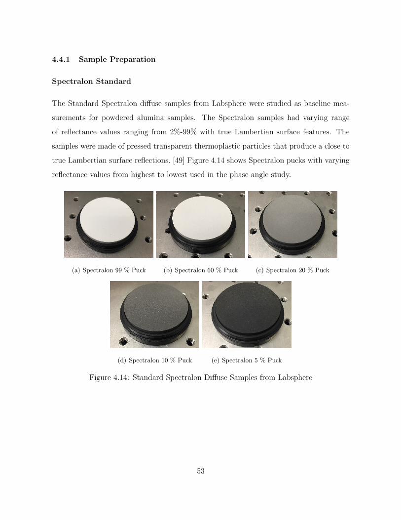
4.4.1 Sample Preparation
Spectralon Standard
The Standard Spectralon diffuse samples from Labsphere were studied as baseline mea-
surements for powdered alumina samples. The Spectralon samples had varying range
of reflectance values ranging from 2%-99% with true Lambertian surface features. The
samples were made of pressed transparent thermoplastic particles that produce a close to
true Lambertian surface reflections. [49] Figure 4.14 shows Spectralon pucks with varying
reflectance values from highest to lowest used in the phase angle study.
(a) Spectralon 99 % Puck (b) Spectralon 60 % Puck (c) Spectralon 20 % Puck
(d) Spectralon 10 % Puck (e) Spectralon 5 % Puck
Figure 4.14: Standard Spectralon Diffuse Samples from Labsphere
53
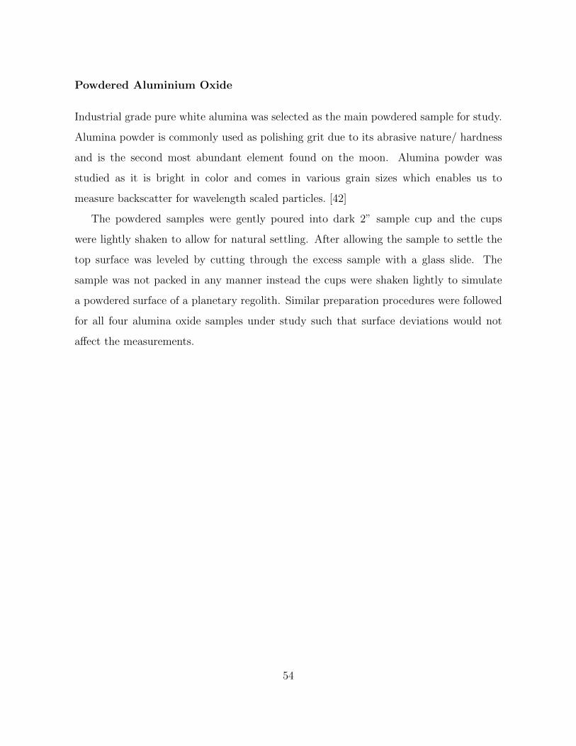
Powdered Aluminium Oxide
Industrial grade pure white alumina was selected as the main powdered sample for study.
Alumina powder is commonly used as polishing grit due to its abrasive nature/ hardness
and is the second most abundant element found on the moon. Alumina powder was
studied as it is bright in color and comes in various grain sizes which enables us to
measure backscatter for wavelength scaled particles. [42]
The powdered samples were gently poured into dark 2” sample cup and the cups
were lightly shaken to allow for natural settling. After allowing the sample to settle the
top surface was leveled by cutting through the excess sample with a glass slide. The
sample was not packed in any manner instead the cups were shaken lightly to simulate
a powdered surface of a planetary regolith. Similar preparation procedures were followed
for all four alumina oxide samples under study such that surface deviations would not
affect the measurements.
54
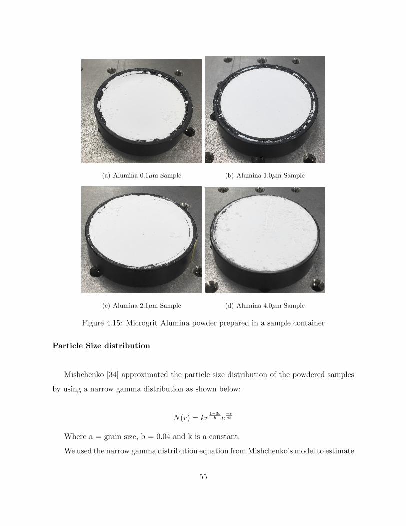
(a) Alumina 0.1µm Sample (b) Alumina 1.0µm Sample
(c) Alumina 2.1µm Sample (d) Alumina 4.0µm Sample
Figure 4.15: Microgrit Alumina powder prepared in a sample container
Particle Size distribution
Mishchenko [34] approximated the particle size distribution of the powdered samples
by using a narrow gamma distribution as shown below:
N(r) = kr1−3b
b e−rab
Where a = grain size, b = 0.04 and k is a constant.
We used the narrow gamma distribution equation from Mishchenko’s model to estimate
55
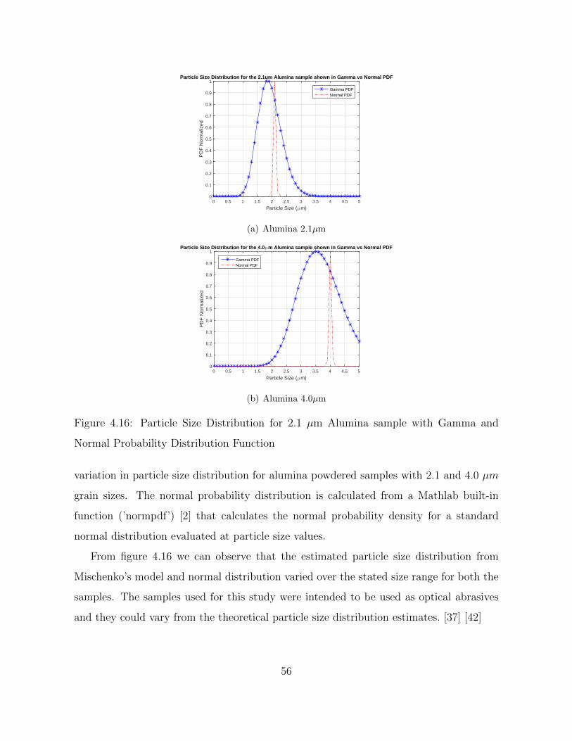
Particle Size (µm)0 0.5 1 1.5 2 2.5 3 3.5 4 4.5 5
PD
F N
orm
aliz
ed0
0.1
0.2
0.3
0.4
0.5
0.6
0.7
0.8
0.9
1Particle Size Distribution for the 2.1um Alumina sample shown in Gamma vs Normal PDF
Gamma PDFNormal PDF
(a) Alumina 2.1µm
Particle Size (µm)0 0.5 1 1.5 2 2.5 3 3.5 4 4.5 5
PD
F N
orm
aliz
ed
0
0.1
0.2
0.3
0.4
0.5
0.6
0.7
0.8
0.9
1Particle Size Distribution for the 4.0µm Alumina sample shown in Gamma vs Normal PDF
Gamma PDFNormal PDF
(b) Alumina 4.0µm
Figure 4.16: Particle Size Distribution for 2.1 µm Alumina sample with Gamma and
Normal Probability Distribution Function
variation in particle size distribution for alumina powdered samples with 2.1 and 4.0 µm
grain sizes. The normal probability distribution is calculated from a Mathlab built-in
function (’normpdf’) [2] that calculates the normal probability density for a standard
normal distribution evaluated at particle size values.
From figure 4.16 we can observe that the estimated particle size distribution from
Mischenko’s model and normal distribution varied over the stated size range for both the
samples. The samples used for this study were intended to be used as optical abrasives
and they could vary from the theoretical particle size distribution estimates. [37] [42]
56
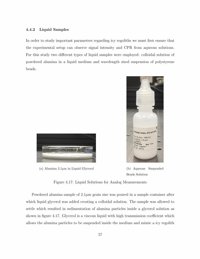
4.4.2 Liquid Samples
In order to study important parameters regarding icy regoliths we must first ensure that
the experimental setup can observe signal intensity and CPR from aqueous solutions.
For this study two different types of liquid samples were employed: colloidal solution of
powdered alumina in a liquid medium and wavelength sized suspension of polystyrene
beads.
(a) Alumina 2.1µm in Liquid Glycerol (b) Aqueous Suspended
Beads Solution
Figure 4.17: Liquid Solutions for Analog Measurements
Powdered alumina sample of 2.1µm grain size was poured in a sample container after
which liquid glycerol was added creating a colloidal solution. The sample was allowed to
settle which resulted in sedimentation of alumina particles inside a glycerol solution as
shown in figure 4.17. Glycerol is a viscous liquid with high transmission coefficient which
allows the alumina particles to be suspended inside the medium and mimic a icy regolith
57

with cracks and rock impurities. Thermo Fisher Scientific manufactures [33] an aqueous
milky white suspension containing polystyrene spheres with nominal diameters of 0.76µm.
Incident signal would undergo change in wavelength propagating from vacuum λ0 to a
liquid medium λl with refractive index (n) resulting in the liquid wavelength of, λl = λ0/n.
For an incident wavelength of 1.064µm, the particle size to wavelength ratio ( d/λ) for
suspended particles in Thermo Fischer solution would be 0.71, and for glycerol/alumina
colloidal solution would be 0.68 which are much smaller than the incident radiation.
58
5 Measurements and Dataset Analysis
5.1 Previous Studies Observing Circular Polarization Ratios
In this section we shall overview the previous studies undertaken related to the experi-
mental near zero phase angle and the implications these studies have on our measurement
setup. There have been several analog CPR and reflectance experiments performed to
study and differentiate the shadow hiding effects. We shall observe some of Nelson’s
published papers and draw implications that are applicable to our current study. [37]
The author measured the change in reflectance and circular polarization ratio with
respect to phase angle of highly reflective aluminum powders for understanding the con-
tribution of coherent backscattering effect on the reflectance phase plots of planetary
regoliths. The schematic for the experiment is shown in the figure 5.1 which utilizes
a goniometric photopolarimeter with phase angle range from 0.05°-5°. The experiment
measures CPR and reflectance for variety of alumina particles sizes ranging from 1µm to
30µm, illuminating the samples from a HeNe laser at 0.633µm wavelength.
59
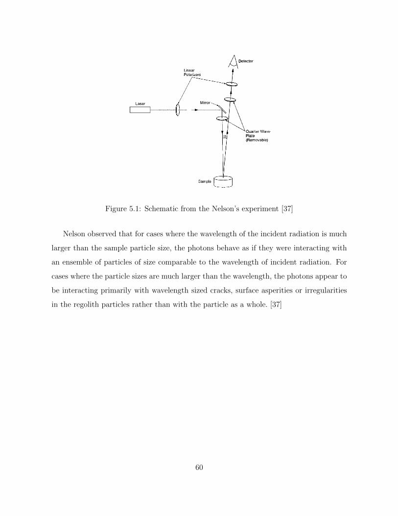
Figure 5.1: Schematic from the Nelson’s experiment [37]
Nelson observed that for cases where the wavelength of the incident radiation is much
larger than the sample particle size, the photons behave as if they were interacting with
an ensemble of particles of size comparable to the wavelength of incident radiation. For
cases where the particle sizes are much larger than the wavelength, the photons appear to
be interacting primarily with wavelength sized cracks, surface asperities or irregularities
in the regolith particles rather than with the particle as a whole. [37]
60
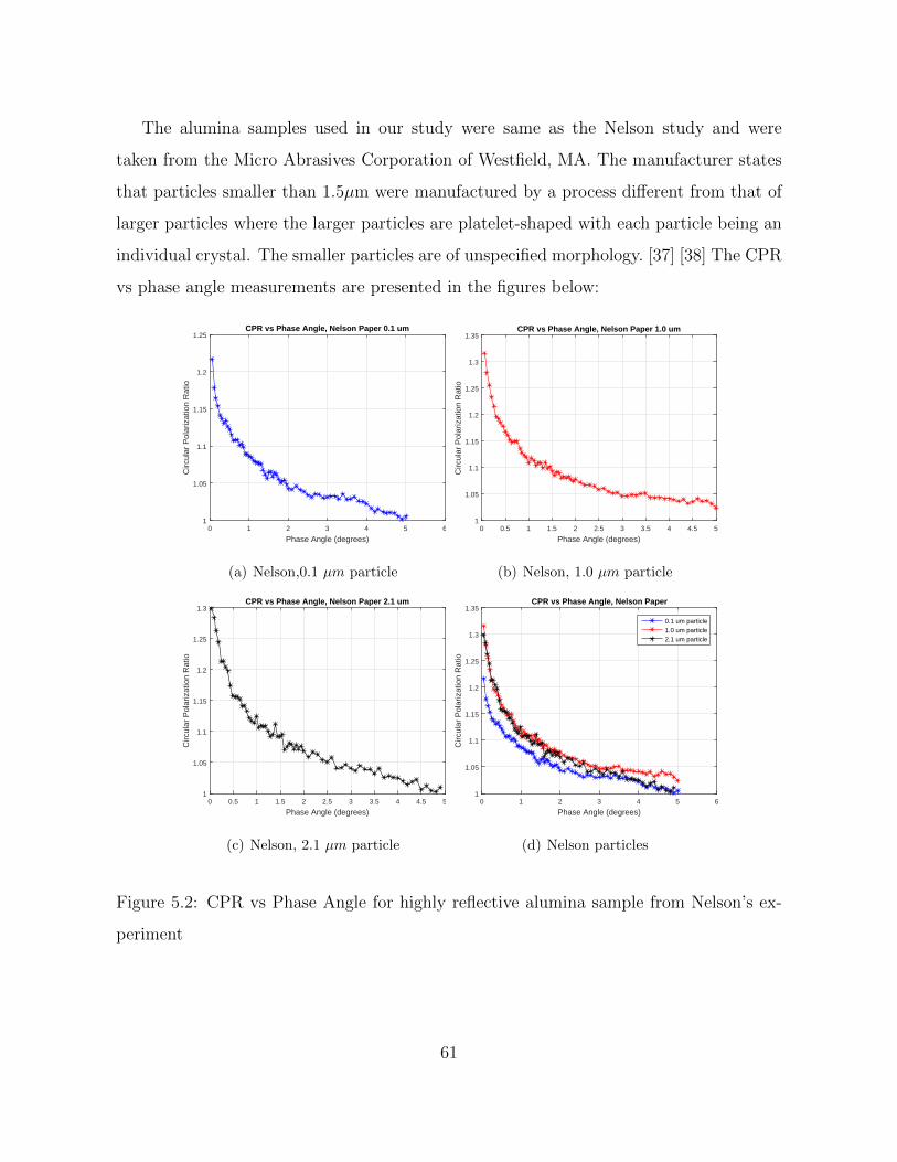
The alumina samples used in our study were same as the Nelson study and were
taken from the Micro Abrasives Corporation of Westfield, MA. The manufacturer states
that particles smaller than 1.5µm were manufactured by a process different from that of
larger particles where the larger particles are platelet-shaped with each particle being an
individual crystal. The smaller particles are of unspecified morphology. [37] [38] The CPR
vs phase angle measurements are presented in the figures below:
Phase Angle (degrees)0 1 2 3 4 5 6
Circ
ular
Pol
ariz
atio
n R
atio
1
1.05
1.1
1.15
1.2
1.25CPR vs Phase Angle, Nelson Paper 0.1 um
(a) Nelson,0.1 µm particle
Phase Angle (degrees)0 0.5 1 1.5 2 2.5 3 3.5 4 4.5 5
Circ
ular
Pol
ariz
atio
n R
atio
1
1.05
1.1
1.15
1.2
1.25
1.3
1.35CPR vs Phase Angle, Nelson Paper 1.0 um
(b) Nelson, 1.0 µm particle
Phase Angle (degrees)0 0.5 1 1.5 2 2.5 3 3.5 4 4.5 5
Circ
ular
Pol
ariz
atio
n R
atio
1
1.05
1.1
1.15
1.2
1.25
1.3CPR vs Phase Angle, Nelson Paper 2.1 um
(c) Nelson, 2.1 µm particle
Phase Angle (degrees)0 1 2 3 4 5 6
Circ
ular
Pol
ariz
atio
n R
atio
1
1.05
1.1
1.15
1.2
1.25
1.3
1.35CPR vs Phase Angle, Nelson Paper
0.1 um particle1.0 um particle2.1 um particle
(d) Nelson particles
Figure 5.2: CPR vs Phase Angle for highly reflective alumina sample from Nelson’s ex-
periment
61

Observing the CPR vs phase angle plots here were some key findings:
• The rate of increase in CPR was largest for cases where the particle size was within
a few wavelength sizes of the incident radiation. This result is consistent with the
hypothesis that CBOE is the principal contributor to the opposition effects. [44]
• In highly reflective particulate materials the size and shape of the phase curve near
0°is influenced by coherent backscattering process. [44]
• Coherent backscattering effects are more enhanced than theoretically predicted for
particle sizes much larger and smaller than the wavelength due to variations in the
size distribution of particles, irregularities on the surfaces and interiors of larger
particles that act as scattering centers. [44]
62
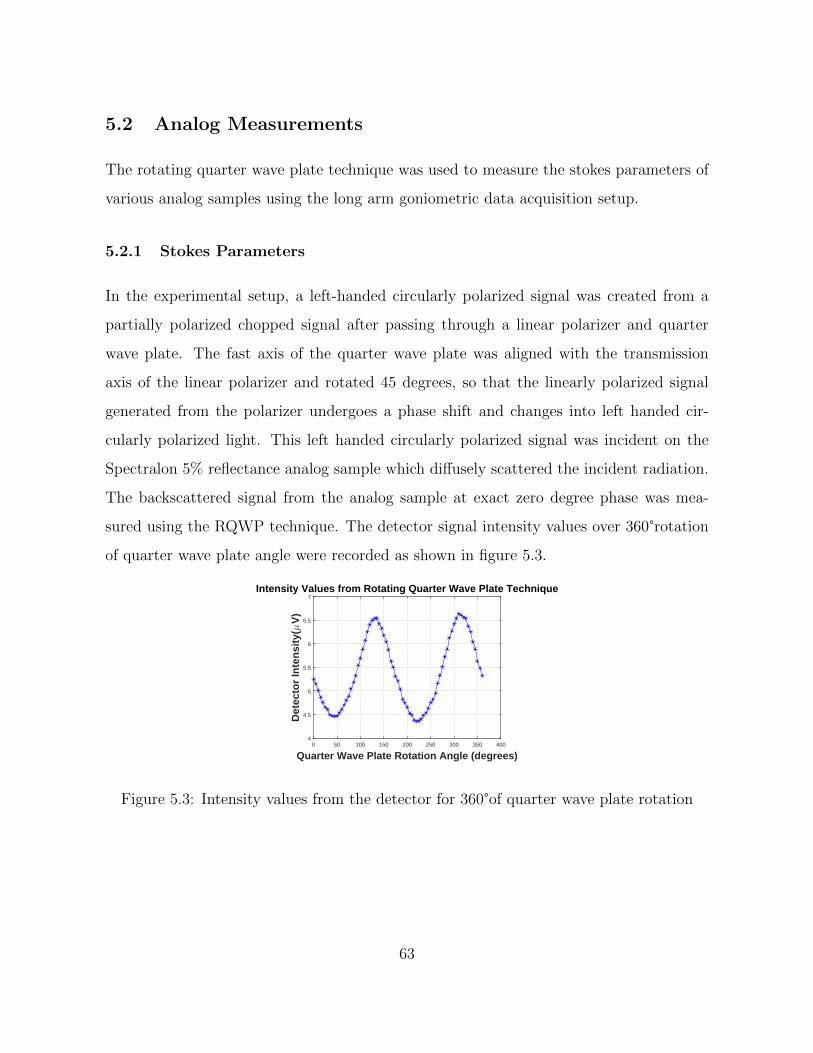
5.2 Analog Measurements
The rotating quarter wave plate technique was used to measure the stokes parameters of
various analog samples using the long arm goniometric data acquisition setup.
5.2.1 Stokes Parameters
In the experimental setup, a left-handed circularly polarized signal was created from a
partially polarized chopped signal after passing through a linear polarizer and quarter
wave plate. The fast axis of the quarter wave plate was aligned with the transmission
axis of the linear polarizer and rotated 45 degrees, so that the linearly polarized signal
generated from the polarizer undergoes a phase shift and changes into left handed cir-
cularly polarized light. This left handed circularly polarized signal was incident on the
Spectralon 5% reflectance analog sample which diffusely scattered the incident radiation.
The backscattered signal from the analog sample at exact zero degree phase was mea-
sured using the RQWP technique. The detector signal intensity values over 360°rotation
of quarter wave plate angle were recorded as shown in figure 5.3.
Quarter Wave Plate Rotation Angle (degrees)0 50 100 150 200 250 300 350 400
Det
ecto
r In
ten
sity
(µV
)
4
4.5
5
5.5
6
6.5
7Intensity Values from Rotating Quarter Wave Plate Technique
Figure 5.3: Intensity values from the detector for 360°of quarter wave plate rotation
63
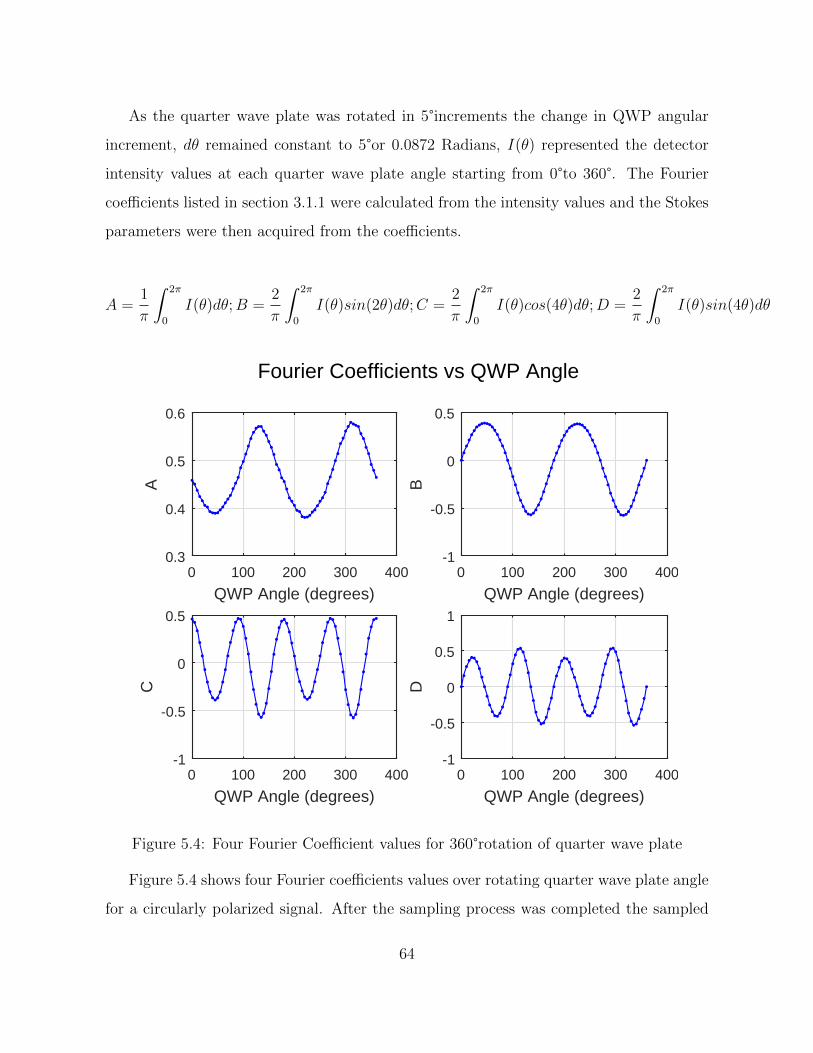
As the quarter wave plate was rotated in 5°increments the change in QWP angular
increment, dθ remained constant to 5°or 0.0872 Radians, I(θ) represented the detector
intensity values at each quarter wave plate angle starting from 0°to 360°. The Fourier
coefficients listed in section 3.1.1 were calculated from the intensity values and the Stokes
parameters were then acquired from the coefficients.
A =1
π
∫ 2π
0
I(θ)dθ;B =2
π
∫ 2π
0
I(θ)sin(2θ)dθ;C =2
π
∫ 2π
0
I(θ)cos(4θ)dθ;D =2
π
∫ 2π
0
I(θ)sin(4θ)dθ
QWP Angle (degrees)0 100 200 300 400
A
0.3
0.4
0.5
0.6
QWP Angle (degrees)0 100 200 300 400
B
-1
-0.5
0
0.5
QWP Angle (degrees)0 100 200 300 400
C
-1
-0.5
0
0.5
Fourier Coefficients vs QWP Angle
QWP Angle (degrees)0 100 200 300 400
D
-1
-0.5
0
0.5
1
Figure 5.4: Four Fourier Coefficient values for 360°rotation of quarter wave plate
Figure 5.4 shows four Fourier coefficients values over rotating quarter wave plate angle
for a circularly polarized signal. After the sampling process was completed the sampled
64
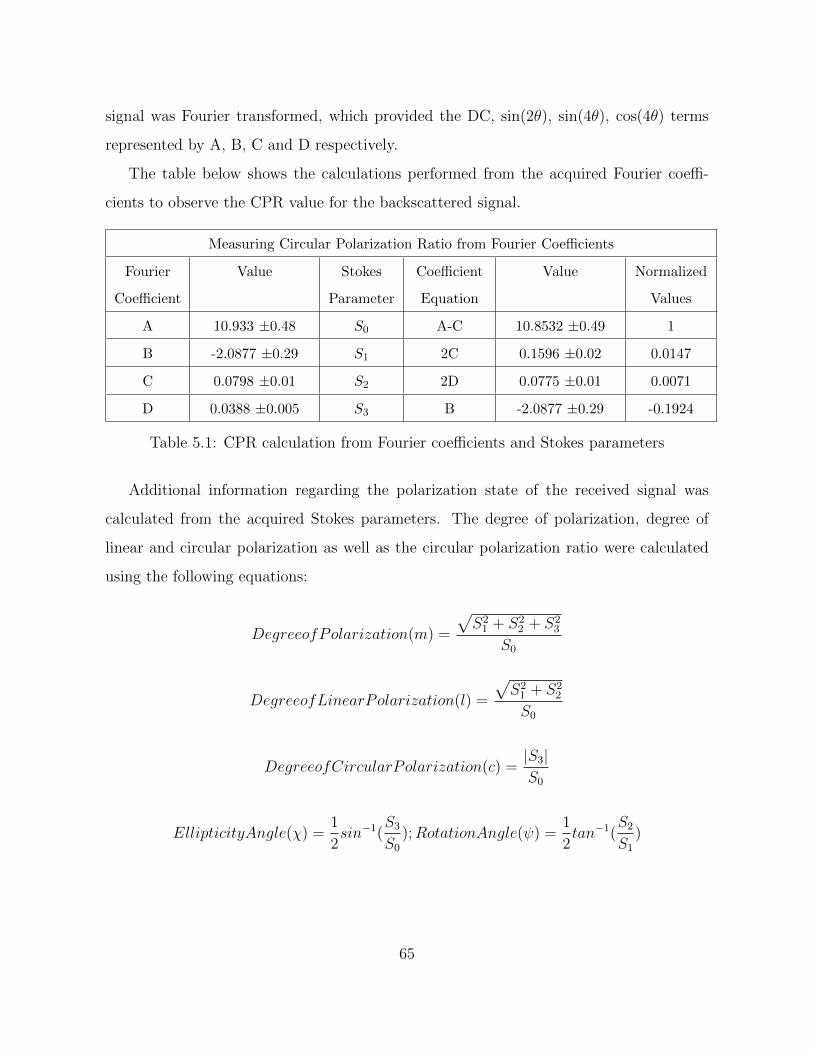
signal was Fourier transformed, which provided the DC, sin(2θ), sin(4θ), cos(4θ) terms
represented by A, B, C and D respectively.
The table below shows the calculations performed from the acquired Fourier coeffi-
cients to observe the CPR value for the backscattered signal.
Measuring Circular Polarization Ratio from Fourier Coefficients
Fourier
Coefficient
Value Stokes
Parameter
Coefficient
Equation
Value Normalized
Values
A 10.933 ±0.48 S0 A-C 10.8532 ±0.49 1
B -2.0877 ±0.29 S1 2C 0.1596 ±0.02 0.0147
C 0.0798 ±0.01 S2 2D 0.0775 ±0.01 0.0071
D 0.0388 ±0.005 S3 B -2.0877 ±0.29 -0.1924
Table 5.1: CPR calculation from Fourier coefficients and Stokes parameters
Additional information regarding the polarization state of the received signal was
calculated from the acquired Stokes parameters. The degree of polarization, degree of
linear and circular polarization as well as the circular polarization ratio were calculated
using the following equations:
DegreeofPolarization(m) =
√S21 + S2
2 + S23
S0
DegreeofLinearPolarization(l) =
√S21 + S2
2
S0
DegreeofCircularPolarization(c) =|S3|S0
EllipticityAngle(χ) =1
2sin−1(
S3
S0
);RotationAngle(ψ) =1
2tan−1(
S2
S1
)
65
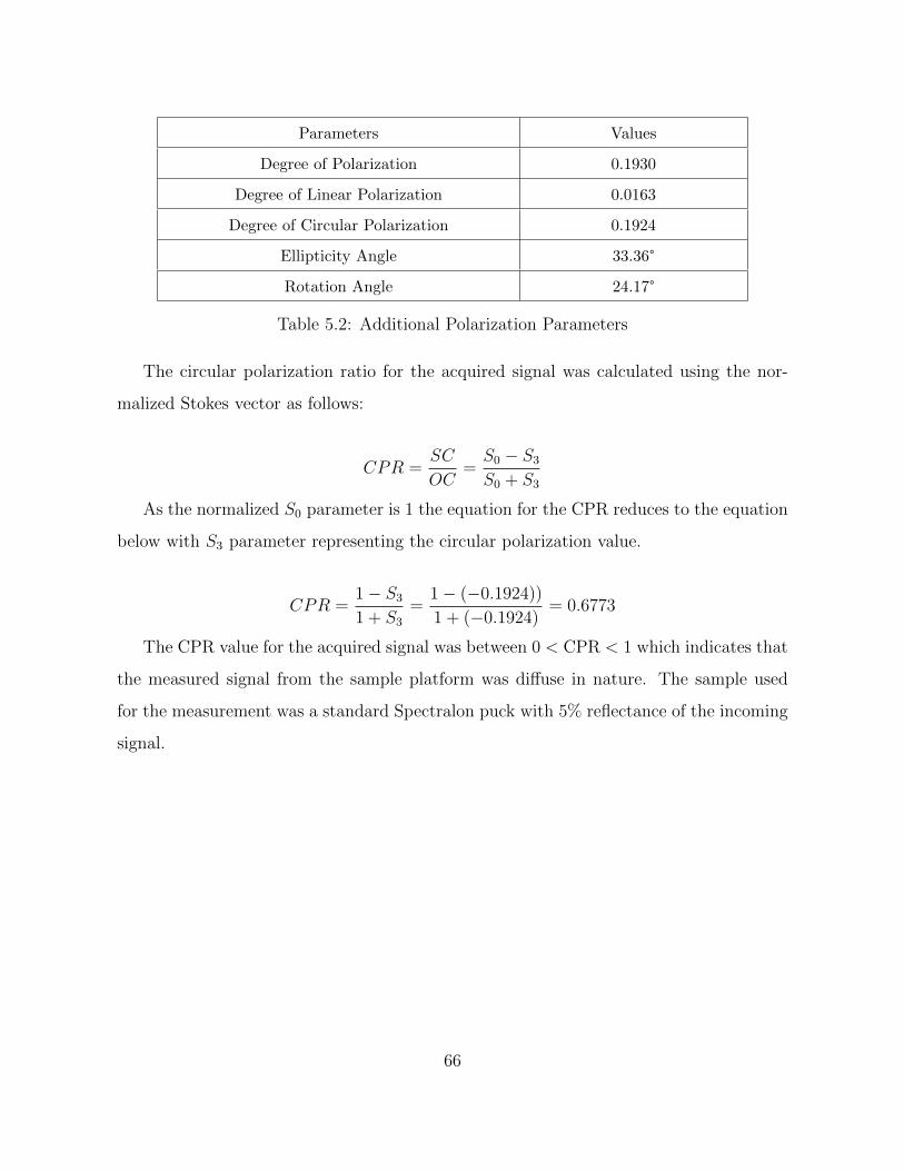
Parameters Values
Degree of Polarization 0.1930
Degree of Linear Polarization 0.0163
Degree of Circular Polarization 0.1924
Ellipticity Angle 33.36°
Rotation Angle 24.17°
Table 5.2: Additional Polarization Parameters
The circular polarization ratio for the acquired signal was calculated using the nor-
malized Stokes vector as follows:
CPR =SC
OC=S0 − S3
S0 + S3
As the normalized S0 parameter is 1 the equation for the CPR reduces to the equation
below with S3 parameter representing the circular polarization value.
CPR =1− S3
1 + S3
=1− (−0.1924))
1 + (−0.1924)= 0.6773
The CPR value for the acquired signal was between 0 < CPR < 1 which indicates that
the measured signal from the sample platform was diffuse in nature. The sample used
for the measurement was a standard Spectralon puck with 5% reflectance of the incoming
signal.
66
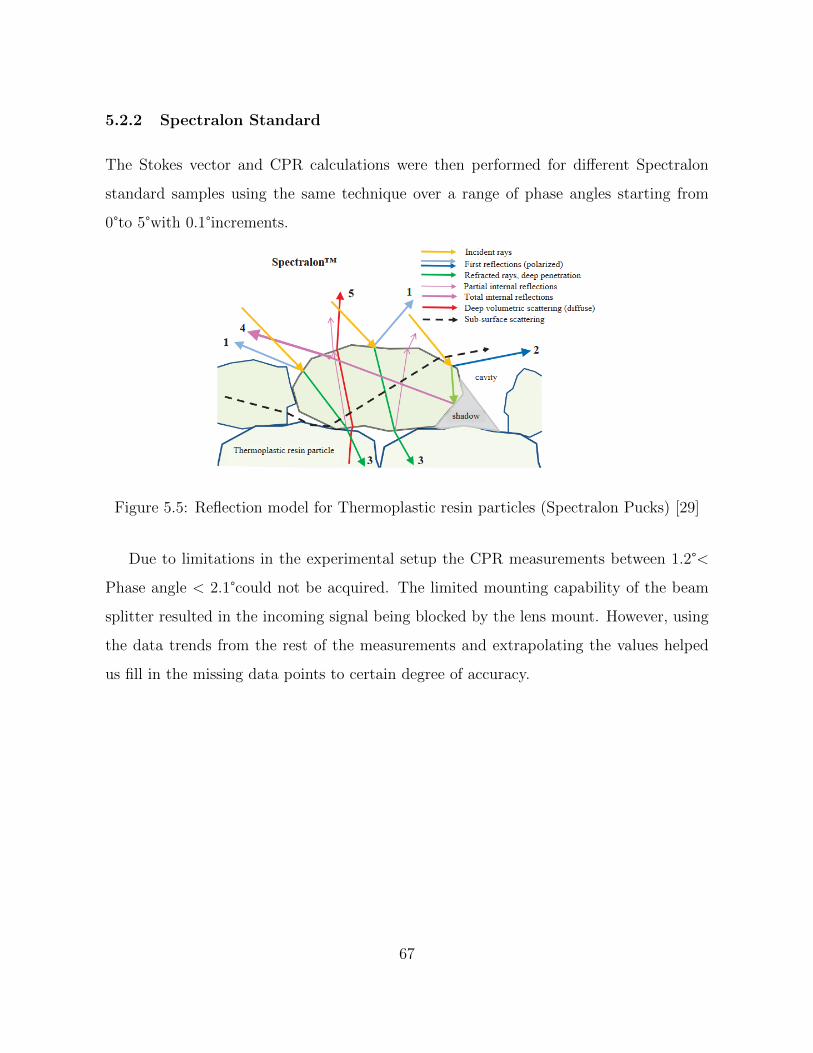
5.2.2 Spectralon Standard
The Stokes vector and CPR calculations were then performed for different Spectralon
standard samples using the same technique over a range of phase angles starting from
0°to 5°with 0.1°increments.
Figure 5.5: Reflection model for Thermoplastic resin particles (Spectralon Pucks) [29]
Due to limitations in the experimental setup the CPR measurements between 1.2°<
Phase angle < 2.1°could not be acquired. The limited mounting capability of the beam
splitter resulted in the incoming signal being blocked by the lens mount. However, using
the data trends from the rest of the measurements and extrapolating the values helped
us fill in the missing data points to certain degree of accuracy.
67
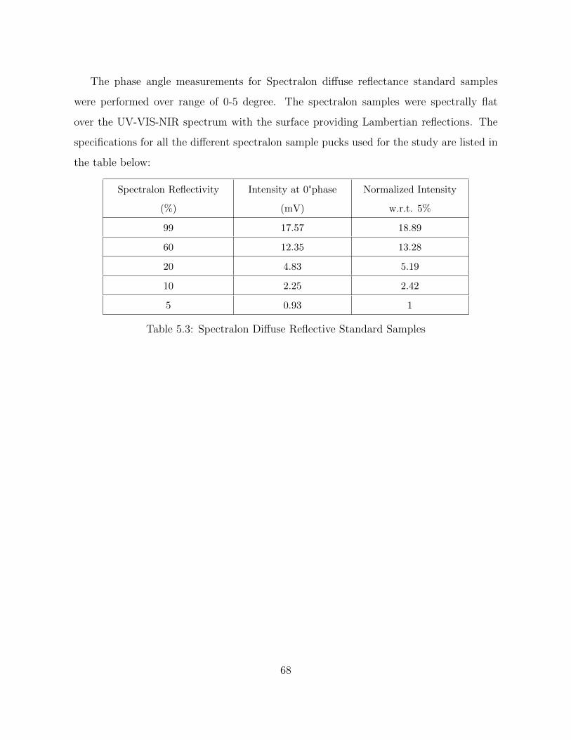
The phase angle measurements for Spectralon diffuse reflectance standard samples
were performed over range of 0-5 degree. The spectralon samples were spectrally flat
over the UV-VIS-NIR spectrum with the surface providing Lambertian reflections. The
specifications for all the different spectralon sample pucks used for the study are listed in
the table below:
Spectralon Reflectivity
(%)
Intensity at 0°phase
(mV)
Normalized Intensity
w.r.t. 5%
99 17.57 18.89
60 12.35 13.28
20 4.83 5.19
10 2.25 2.42
5 0.93 1
Table 5.3: Spectralon Diffuse Reflective Standard Samples
68
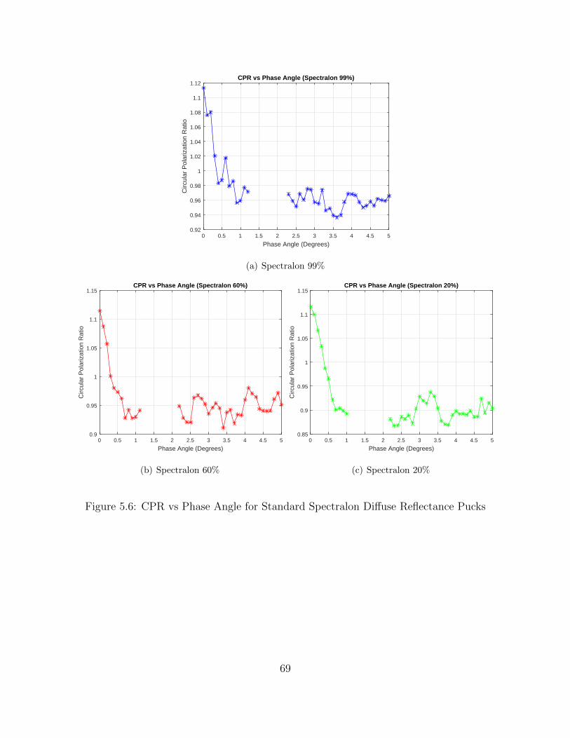
Phase Angle (Degrees)0 0.5 1 1.5 2 2.5 3 3.5 4 4.5 5
Circ
ular
Pol
ariz
atio
n R
atio
0.92
0.94
0.96
0.98
1
1.02
1.04
1.06
1.08
1.1
1.12CPR vs Phase Angle (Spectralon 99%)
(a) Spectralon 99%
Phase Angle (Degrees)0 0.5 1 1.5 2 2.5 3 3.5 4 4.5 5
Circ
ular
Pol
ariz
atio
n R
atio
0.9
0.95
1
1.05
1.1
1.15CPR vs Phase Angle (Spectralon 60%)
(b) Spectralon 60%
Phase Angle (Degrees)0 0.5 1 1.5 2 2.5 3 3.5 4 4.5 5
Circ
ular
Pol
ariz
atio
n R
atio
0.85
0.9
0.95
1
1.05
1.1
1.15CPR vs Phase Angle (Spectralon 20%)
(c) Spectralon 20%
Figure 5.6: CPR vs Phase Angle for Standard Spectralon Diffuse Reflectance Pucks
69
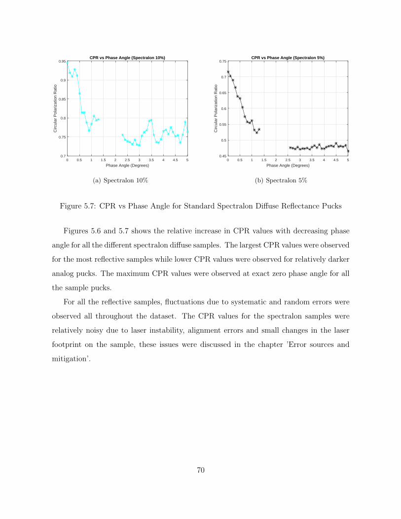
Phase Angle (Degrees)0 0.5 1 1.5 2 2.5 3 3.5 4 4.5 5
Circ
ular
Pol
ariz
atio
n R
atio
0.7
0.75
0.8
0.85
0.9
0.95CPR vs Phase Angle (Spectralon 10%)
(a) Spectralon 10%
Phase Angle (Degrees)0 0.5 1 1.5 2 2.5 3 3.5 4 4.5 5
Circ
ular
Pol
ariz
atio
n R
atio
0.45
0.5
0.55
0.6
0.65
0.7
0.75CPR vs Phase Angle (Spectralon 5%)
(b) Spectralon 5%
Figure 5.7: CPR vs Phase Angle for Standard Spectralon Diffuse Reflectance Pucks
Figures 5.6 and 5.7 shows the relative increase in CPR values with decreasing phase
angle for all the different spectralon diffuse samples. The largest CPR values were observed
for the most reflective samples while lower CPR values were observed for relatively darker
analog pucks. The maximum CPR values were observed at exact zero phase angle for all
the sample pucks.
For all the reflective samples, fluctuations due to systematic and random errors were
observed all throughout the dataset. The CPR values for the spectralon samples were
relatively noisy due to laser instability, alignment errors and small changes in the laser
footprint on the sample, these issues were discussed in the chapter ’Error sources and
mitigation’.
70
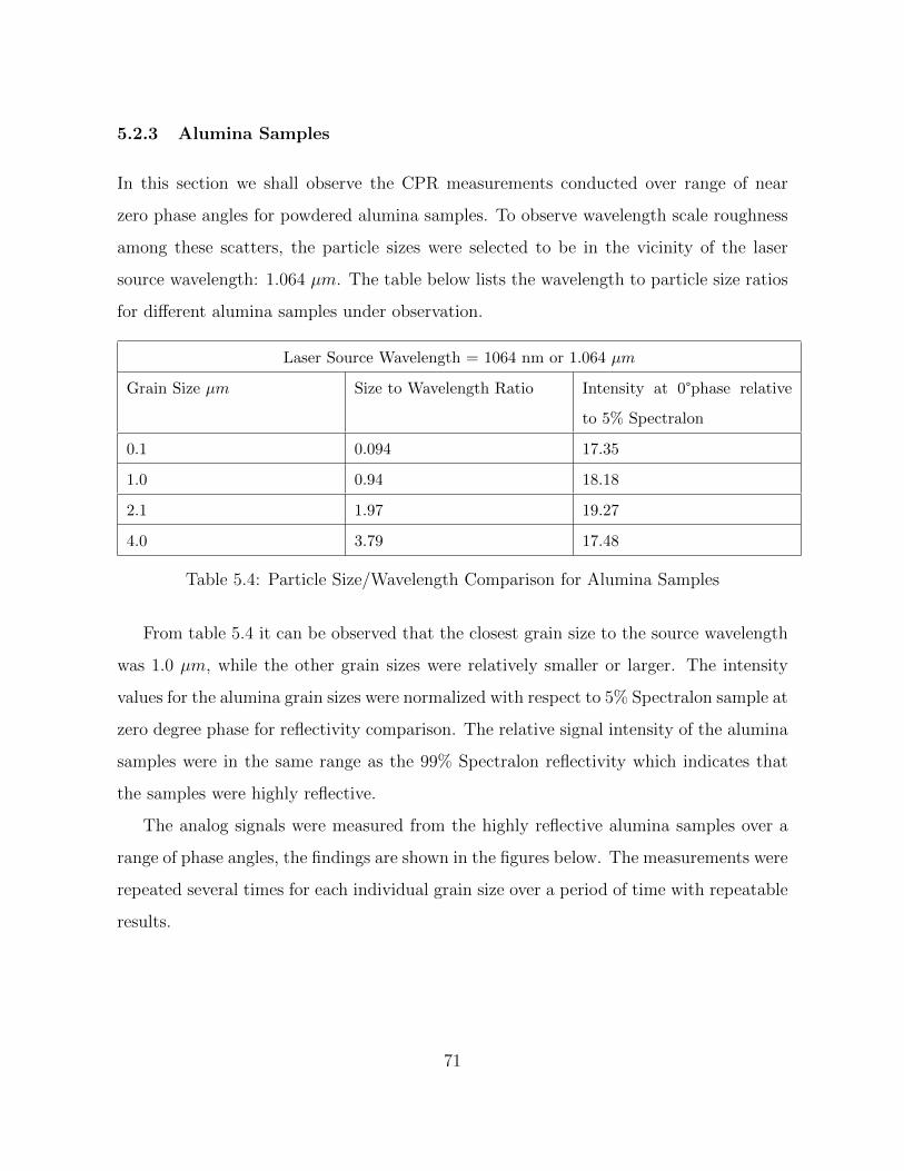
5.2.3 Alumina Samples
In this section we shall observe the CPR measurements conducted over range of near
zero phase angles for powdered alumina samples. To observe wavelength scale roughness
among these scatters, the particle sizes were selected to be in the vicinity of the laser
source wavelength: 1.064 µm. The table below lists the wavelength to particle size ratios
for different alumina samples under observation.
Laser Source Wavelength = 1064 nm or 1.064 µm
Grain Size µm Size to Wavelength Ratio Intensity at 0°phase relative
to 5% Spectralon
0.1 0.094 17.35
1.0 0.94 18.18
2.1 1.97 19.27
4.0 3.79 17.48
Table 5.4: Particle Size/Wavelength Comparison for Alumina Samples
From table 5.4 it can be observed that the closest grain size to the source wavelength
was 1.0 µm, while the other grain sizes were relatively smaller or larger. The intensity
values for the alumina grain sizes were normalized with respect to 5% Spectralon sample at
zero degree phase for reflectivity comparison. The relative signal intensity of the alumina
samples were in the same range as the 99% Spectralon reflectivity which indicates that
the samples were highly reflective.
The analog signals were measured from the highly reflective alumina samples over a
range of phase angles, the findings are shown in the figures below. The measurements were
repeated several times for each individual grain size over a period of time with repeatable
results.
71
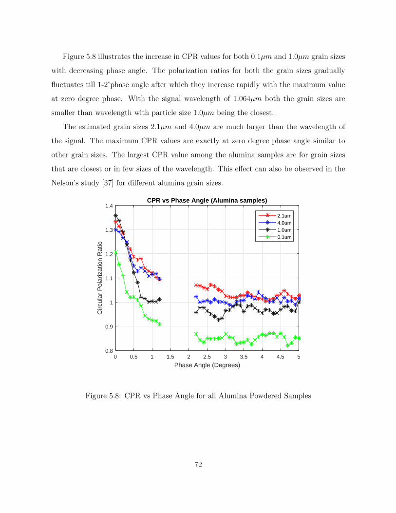
Figure 5.8 illustrates the increase in CPR values for both 0.1µm and 1.0µm grain sizes
with decreasing phase angle. The polarization ratios for both the grain sizes gradually
fluctuates till 1-2°phase angle after which they increase rapidly with the maximum value
at zero degree phase. With the signal wavelength of 1.064µm both the grain sizes are
smaller than wavelength with particle size 1.0µm being the closest.
The estimated grain sizes 2.1µm and 4.0µm are much larger than the wavelength of
the signal. The maximum CPR values are exactly at zero degree phase angle similar to
other grain sizes. The largest CPR value among the alumina samples are for grain sizes
that are closest or in few sizes of the wavelength. This effect can also be observed in the
Nelson’s study [37] for different alumina grain sizes.
Phase Angle (Degrees)0 0.5 1 1.5 2 2.5 3 3.5 4 4.5 5
Circ
ular
Pol
ariz
atio
n R
atio
0.8
0.9
1
1.1
1.2
1.3
1.4CPR vs Phase Angle (Alumina samples)
2.1um4.0um1.0um0.1um
Figure 5.8: CPR vs Phase Angle for all Alumina Powdered Samples
72
For particle sizes much larger than the wavelength of the incident signal, the minimum
CPR values are at much larger phase angles compared to the particle sizes that are close
to the wavelength of the signal. For particle sizes much smaller than the incident wave-
length, the minimum CPR was much lower in value than the other particle sizes. The
CPR maximum was highest for the particle size closest to the wavelength of the incident
signal, 1.0µm while the lowest CPR was for the smallest particle size, 0.1µm.
From the observed CPR trends we can validate the presence of opposition effects
mainly the coherent backscattering effect. For all the highly reflective alumina samples,
large polarized opposition surges at near zero phase angle which are indicative of the
opposition effects were observed. Moreover, the high CPR values near zero phase which
implies that the same sense of polarized signal were observed that occur due to multiple
scattering instead of single reflected light.
73
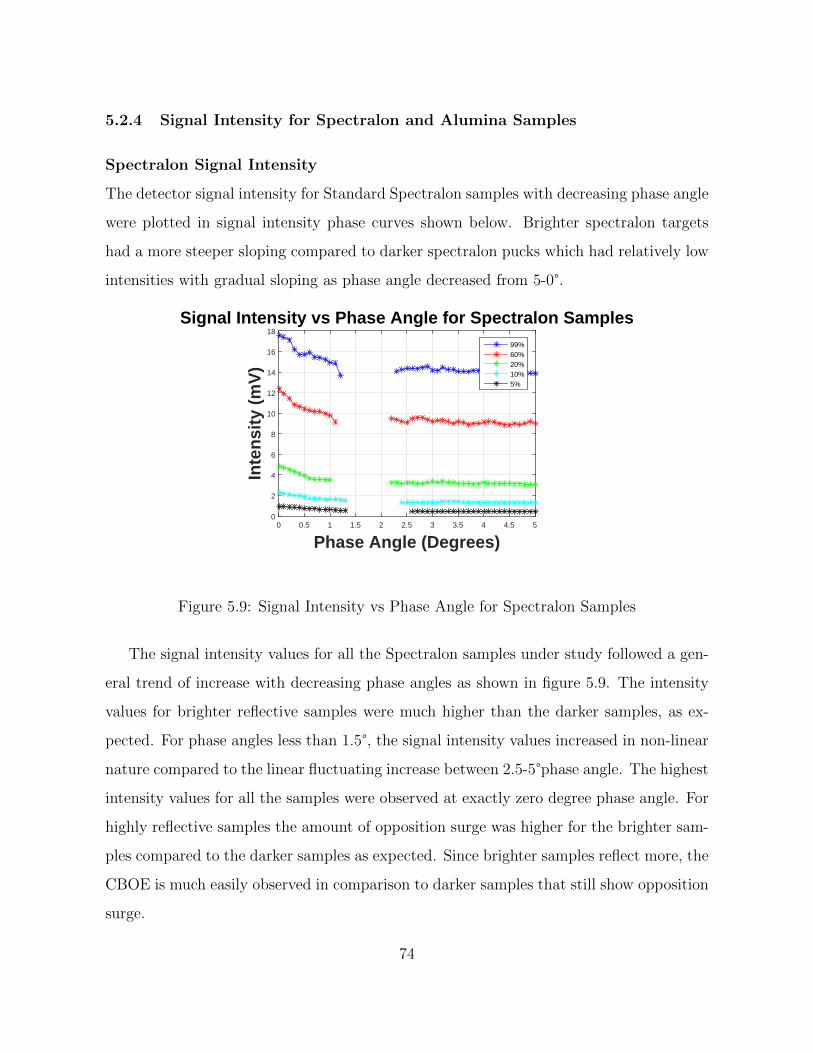
5.2.4 Signal Intensity for Spectralon and Alumina Samples
Spectralon Signal Intensity
The detector signal intensity for Standard Spectralon samples with decreasing phase angle
were plotted in signal intensity phase curves shown below. Brighter spectralon targets
had a more steeper sloping compared to darker spectralon pucks which had relatively low
intensities with gradual sloping as phase angle decreased from 5-0°.
Phase Angle (Degrees)0 0.5 1 1.5 2 2.5 3 3.5 4 4.5 5
Inte
nsi
ty (
mV
)
0
2
4
6
8
10
12
14
16
18Signal Intensity vs Phase Angle for Spectralon Samples
99%60%20%10%5%
Figure 5.9: Signal Intensity vs Phase Angle for Spectralon Samples
The signal intensity values for all the Spectralon samples under study followed a gen-
eral trend of increase with decreasing phase angles as shown in figure 5.9. The intensity
values for brighter reflective samples were much higher than the darker samples, as ex-
pected. For phase angles less than 1.5°, the signal intensity values increased in non-linear
nature compared to the linear fluctuating increase between 2.5-5°phase angle. The highest
intensity values for all the samples were observed at exactly zero degree phase angle. For
highly reflective samples the amount of opposition surge was higher for the brighter sam-
ples compared to the darker samples as expected. Since brighter samples reflect more, the
CBOE is much easily observed in comparison to darker samples that still show opposition
surge.
74
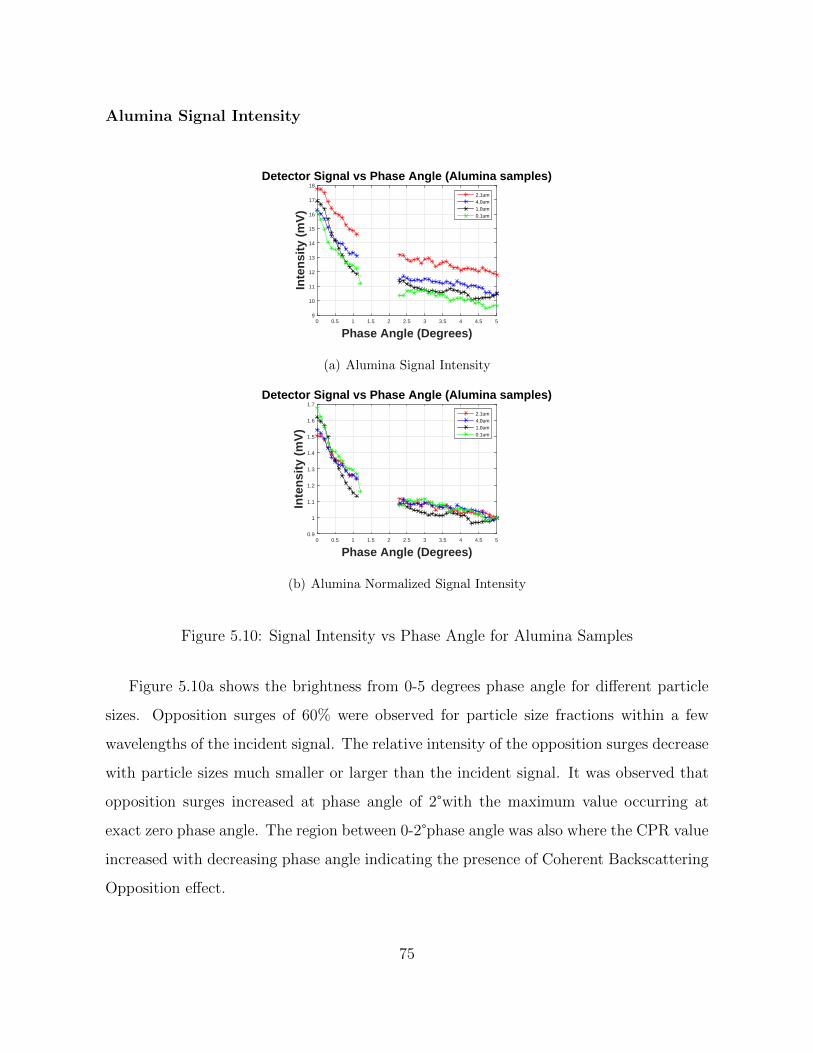
Alumina Signal Intensity
Phase Angle (Degrees)0 0.5 1 1.5 2 2.5 3 3.5 4 4.5 5
Inte
nsi
ty (
mV
)9
10
11
12
13
14
15
16
17
18Detector Signal vs Phase Angle (Alumina samples)
2.1um4.0um1.0um0.1um
(a) Alumina Signal Intensity
Phase Angle (Degrees)0 0.5 1 1.5 2 2.5 3 3.5 4 4.5 5
Inte
nsi
ty (
mV
)
0.9
1
1.1
1.2
1.3
1.4
1.5
1.6
1.7Detector Signal vs Phase Angle (Alumina samples)
2.1um4.0um1.0um0.1um
(b) Alumina Normalized Signal Intensity
Figure 5.10: Signal Intensity vs Phase Angle for Alumina Samples
Figure 5.10a shows the brightness from 0-5 degrees phase angle for different particle
sizes. Opposition surges of 60% were observed for particle size fractions within a few
wavelengths of the incident signal. The relative intensity of the opposition surges decrease
with particle sizes much smaller or larger than the incident signal. It was observed that
opposition surges increased at phase angle of 2°with the maximum value occurring at
exact zero phase angle. The region between 0-2°phase angle was also where the CPR value
increased with decreasing phase angle indicating the presence of Coherent Backscattering
Opposition effect.
75
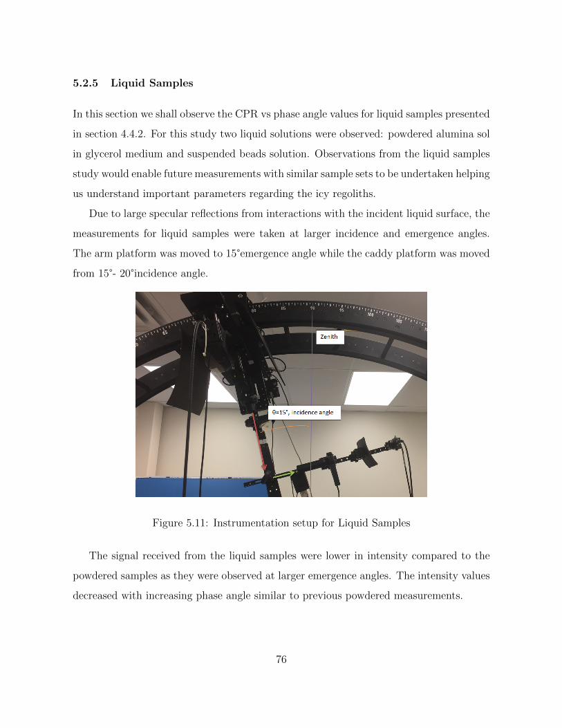
5.2.5 Liquid Samples
In this section we shall observe the CPR vs phase angle values for liquid samples presented
in section 4.4.2. For this study two liquid solutions were observed: powdered alumina sol
in glycerol medium and suspended beads solution. Observations from the liquid samples
study would enable future measurements with similar sample sets to be undertaken helping
us understand important parameters regarding the icy regoliths.
Due to large specular reflections from interactions with the incident liquid surface, the
measurements for liquid samples were taken at larger incidence and emergence angles.
The arm platform was moved to 15°emergence angle while the caddy platform was moved
from 15°- 20°incidence angle.
Figure 5.11: Instrumentation setup for Liquid Samples
The signal received from the liquid samples were lower in intensity compared to the
powdered samples as they were observed at larger emergence angles. The intensity values
decreased with increasing phase angle similar to previous powdered measurements.
76
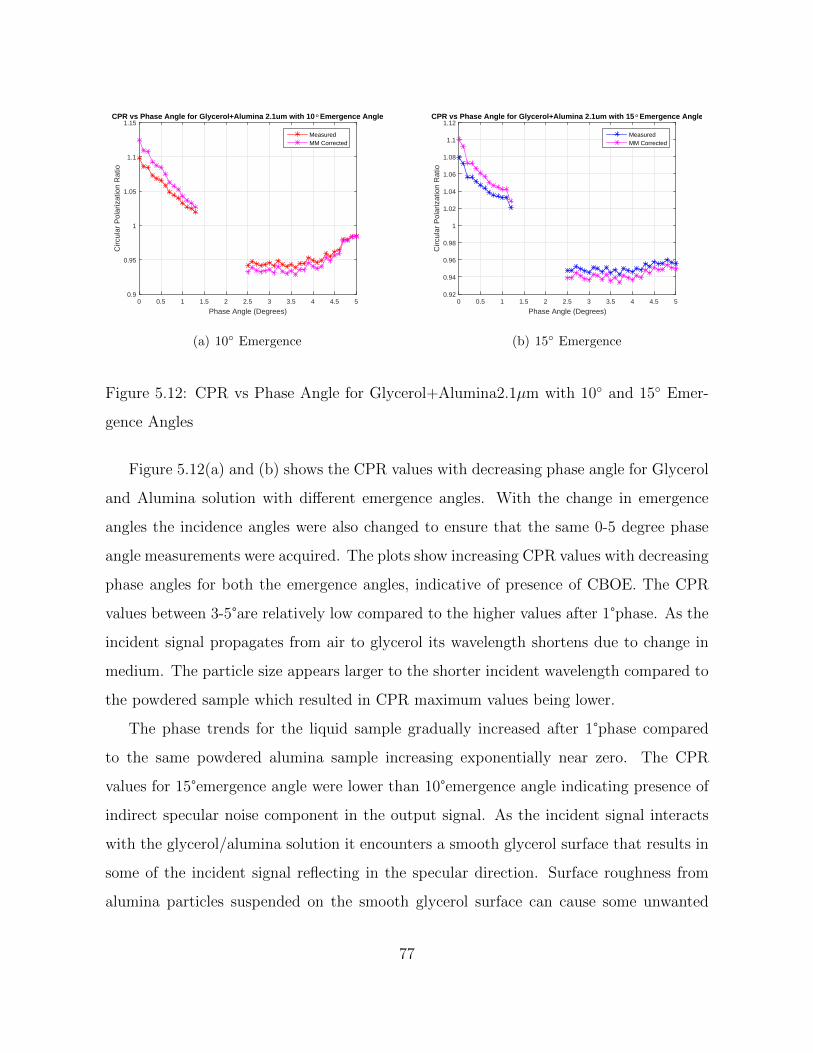
Phase Angle (Degrees)0 0.5 1 1.5 2 2.5 3 3.5 4 4.5 5
Circ
ular
Pol
ariz
atio
n R
atio
0.9
0.95
1
1.05
1.1
1.15CPR vs Phase Angle for Glycerol+Alumina 2.1um with 10° Emergence Angle
MeasuredMM Corrected
(a) 10 Emergence
Phase Angle (Degrees)0 0.5 1 1.5 2 2.5 3 3.5 4 4.5 5
Circ
ular
Pol
ariz
atio
n R
atio
0.92
0.94
0.96
0.98
1
1.02
1.04
1.06
1.08
1.1
1.12CPR vs Phase Angle for Glycerol+Alumina 2.1um with 15° Emergence Angle
MeasuredMM Corrected
(b) 15 Emergence
Figure 5.12: CPR vs Phase Angle for Glycerol+Alumina2.1µm with 10 and 15 Emer-
gence Angles
Figure 5.12(a) and (b) shows the CPR values with decreasing phase angle for Glycerol
and Alumina solution with different emergence angles. With the change in emergence
angles the incidence angles were also changed to ensure that the same 0-5 degree phase
angle measurements were acquired. The plots show increasing CPR values with decreasing
phase angles for both the emergence angles, indicative of presence of CBOE. The CPR
values between 3-5°are relatively low compared to the higher values after 1°phase. As the
incident signal propagates from air to glycerol its wavelength shortens due to change in
medium. The particle size appears larger to the shorter incident wavelength compared to
the powdered sample which resulted in CPR maximum values being lower.
The phase trends for the liquid sample gradually increased after 1°phase compared
to the same powdered alumina sample increasing exponentially near zero. The CPR
values for 15°emergence angle were lower than 10°emergence angle indicating presence of
indirect specular noise component in the output signal. As the incident signal interacts
with the glycerol/alumina solution it encounters a smooth glycerol surface that results in
some of the incident signal reflecting in the specular direction. Surface roughness from
alumina particles suspended on the smooth glycerol surface can cause some unwanted
77
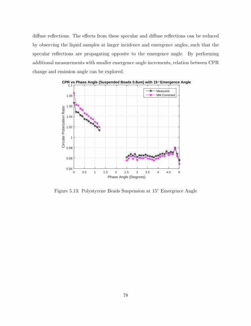
diffuse reflections. The effects from these specular and diffuse reflections can be reduced
by observing the liquid samples at larger incidence and emergence angles, such that the
specular reflections are propagating opposite to the emergence angle. By performing
additional measurements with smaller emergence angle increments, relation between CPR
change and emission angle can be explored.
Phase Angle (Degrees)0 0.5 1 1.5 2 2.5 3 3.5 4 4.5 5
Circ
ular
Pol
ariz
atio
n R
atio
0.94
0.96
0.98
1
1.02
1.04
1.06
1.08
1.1CPR vs Phase Angle (Suspended Beads 0.8um) with 15° Emergence Angle
MeasuredMM Corrected
Figure 5.13: Polystyrene Beads Suspension at 15 Emergence Angle
78
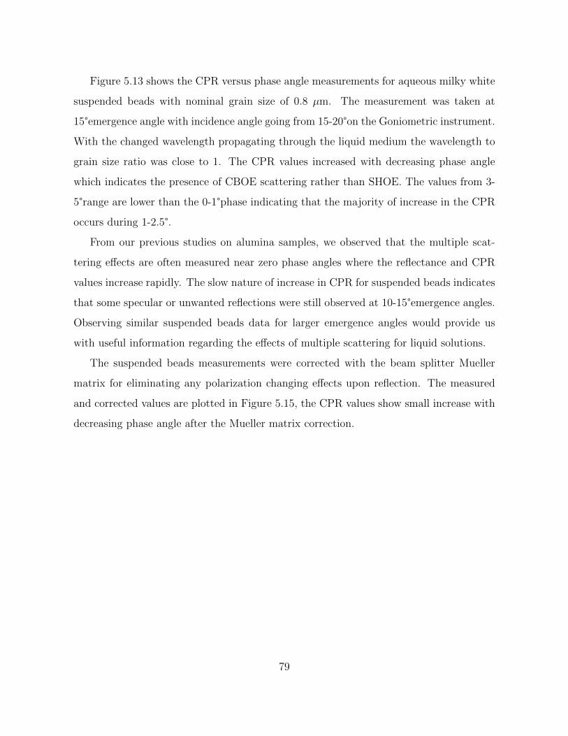
Figure 5.13 shows the CPR versus phase angle measurements for aqueous milky white
suspended beads with nominal grain size of 0.8 µm. The measurement was taken at
15°emergence angle with incidence angle going from 15-20°on the Goniometric instrument.
With the changed wavelength propagating through the liquid medium the wavelength to
grain size ratio was close to 1. The CPR values increased with decreasing phase angle
which indicates the presence of CBOE scattering rather than SHOE. The values from 3-
5°range are lower than the 0-1°phase indicating that the majority of increase in the CPR
occurs during 1-2.5°.
From our previous studies on alumina samples, we observed that the multiple scat-
tering effects are often measured near zero phase angles where the reflectance and CPR
values increase rapidly. The slow nature of increase in CPR for suspended beads indicates
that some specular or unwanted reflections were still observed at 10-15°emergence angles.
Observing similar suspended beads data for larger emergence angles would provide us
with useful information regarding the effects of multiple scattering for liquid solutions.
The suspended beads measurements were corrected with the beam splitter Mueller
matrix for eliminating any polarization changing effects upon reflection. The measured
and corrected values are plotted in Figure 5.15, the CPR values show small increase with
decreasing phase angle after the Mueller matrix correction.
79
5.3 Mueller Matrix Measurements
In the experimental setup, the incoming signal was propagated and reflected through the
beam splitter mounted on the arm platform. Several inconsistencies were measured from
the received backscatter due to uneven s and p polarization reflections from the beam
splitter. These inconsistencies would change the Stokes parameter of the signal when
interacting with the beam splitter. The polarization change caused by the beam splitter
on the signal was analyzed using the Mueller matrix of the beam splitter.
Figure 5.14: Variations in the polarized signal propagating and reflecting from the beam
splitter
Figure 5.14 shows the signal propagating through the beam splitter before and af-
ter interacting with the sample platform with individual polarization states represented
through different Stokes vector. The incoming signal Si1 was right/left handed circularly
polarized which changes its polarization state after propagating through the beam splitter
to So1. After diffused scattering from the sample platform the backscattered signal can
be represented as an incoming signal towards the beam splitter as Si2. The signal changes
its polarization state to So2 after reflecting from the 45°angled beam splitter. The beam
splitter changes the polarization state of the signal twice, this change can be measured by
80
observing the Mueller matrix of the beam splitter. The relationship between the different
polarization states of the signal are as follows:
So1 = M1 ∗ Si1; Si1 = inv(M1) ∗ So1
So2 = M2 ∗ Si2; Si2 = inv(M2) ∗ So2
Where M1 and M2 are Mueller matrices of the beam splitter.
The Mueller matrix of the beam splitter was calculated for the first case where the
incoming signal propagated through the beam splitter and was incident on the sample
platform. Using the dual rotating quarter wave plate technique the intensity values were
measured and Fourier analyzed to calculate the Mueller matrix as shown in section 3.2.1.
M1 =
1 −0.0401 0.2138 0.0032
−0.0453 0.7694 −0.0033 −0.0003
0.0017 −0.0033 0.7601 0.0008
0.0069 0.0112 −0.0165 0.8763
The Mueller matrix M1 resembles the no sample identity matrix from the calibration
procedure. A signal propagating through the beam splitter would retain much of its linear
and circular polarization state as the diagonal elements are positive and close to unity
while the off-diagonal elements are near zero. This implies that the polarization state of
the circularly polarized signal So1 incident on the sample platform would be similar to the
polarization state of the signal Si1 generated from the polarizer and quarter wave plate.
For a completely circularly polarized signal propagating through the beam splitter, 87 %
of the polarization state will be retained.
Secondly, using the observed backscatter signal So2 and the second Mueller matrix M2,
the original diffused signal Si2 from the sample surface was calculated. By calculating
the polarization state of the signal before it reflected from the beam splitter eliminated
the effects of polarization change from the beam splitter. The method of eliminating the
81
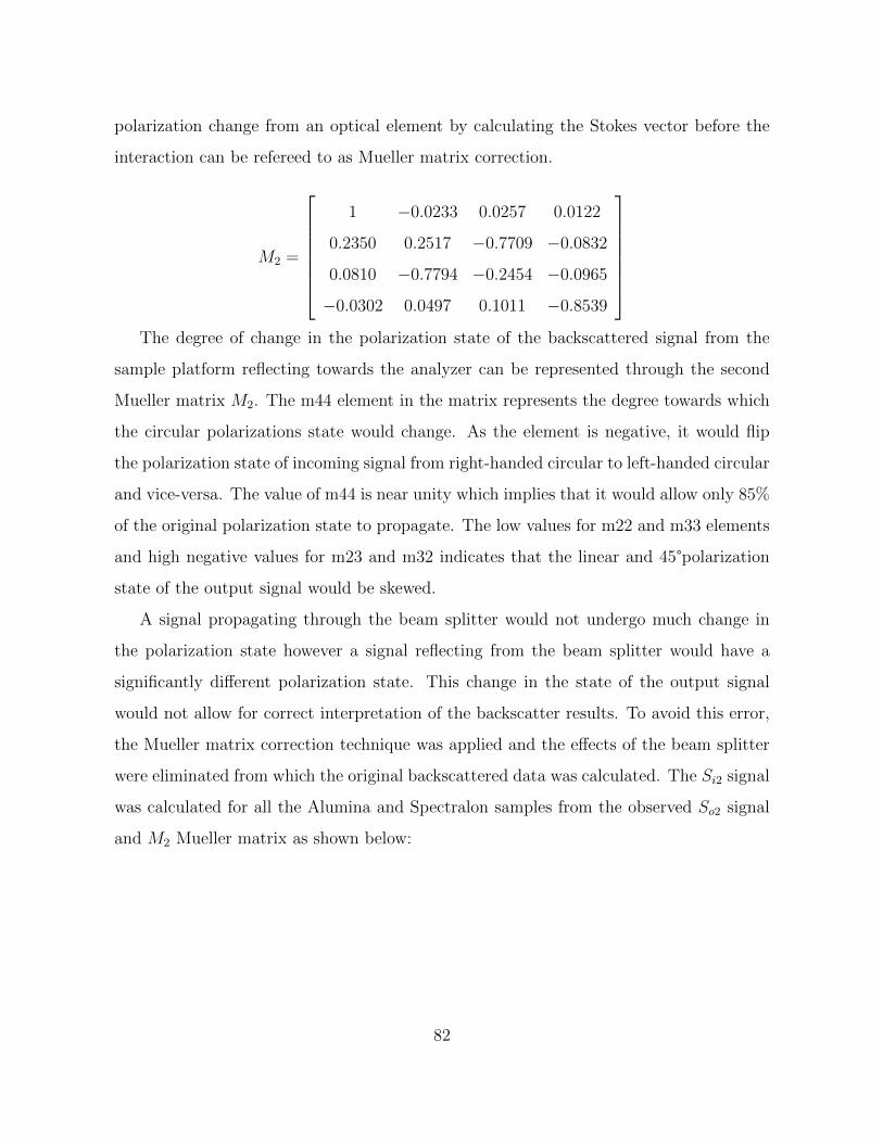
polarization change from an optical element by calculating the Stokes vector before the
interaction can be refereed to as Mueller matrix correction.
M2 =
1 −0.0233 0.0257 0.0122
0.2350 0.2517 −0.7709 −0.0832
0.0810 −0.7794 −0.2454 −0.0965
−0.0302 0.0497 0.1011 −0.8539
The degree of change in the polarization state of the backscattered signal from the
sample platform reflecting towards the analyzer can be represented through the second
Mueller matrix M2. The m44 element in the matrix represents the degree towards which
the circular polarizations state would change. As the element is negative, it would flip
the polarization state of incoming signal from right-handed circular to left-handed circular
and vice-versa. The value of m44 is near unity which implies that it would allow only 85%
of the original polarization state to propagate. The low values for m22 and m33 elements
and high negative values for m23 and m32 indicates that the linear and 45°polarization
state of the output signal would be skewed.
A signal propagating through the beam splitter would not undergo much change in
the polarization state however a signal reflecting from the beam splitter would have a
significantly different polarization state. This change in the state of the output signal
would not allow for correct interpretation of the backscatter results. To avoid this error,
the Mueller matrix correction technique was applied and the effects of the beam splitter
were eliminated from which the original backscattered data was calculated. The Si2 signal
was calculated for all the Alumina and Spectralon samples from the observed So2 signal
and M2 Mueller matrix as shown below:
82
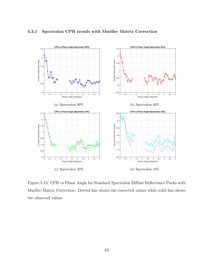
5.3.1 Spectralon CPR trends with Mueller Matrix Correction
Phase Angle (Degrees)0 0.5 1 1.5 2 2.5 3 3.5 4 4.5 5
Circ
ular
Pol
ariz
atio
n R
atio
0.9
0.95
1
1.05
1.1
1.15CPR vs Phase Angle (Spectralon 99%)
(a) Spectralon 99%
Phase Angle (Degrees)0 0.5 1 1.5 2 2.5 3 3.5 4 4.5 5
Circ
ular
Pol
ariz
atio
n R
atio
0.85
0.9
0.95
1
1.05
1.1
1.15CPR vs Phase Angle (Spectralon 60%)
(b) Spectralon 60%
Phase Angle (Degrees)0 0.5 1 1.5 2 2.5 3 3.5 4 4.5 5
Circ
ular
Pol
ariz
atio
n R
atio
0.8
0.85
0.9
0.95
1
1.05
1.1
1.15CPR vs Phase Angle (Spectralon 20%)
(c) Spectralon 20%
Phase Angle (Degrees)0 0.5 1 1.5 2 2.5 3 3.5 4 4.5 5
Circ
ular
Pol
ariz
atio
n R
atio
0.65
0.7
0.75
0.8
0.85
0.9
0.95CPR vs Phase Angle (Spectralon 10%)
(d) Spectralon 10%
Figure 5.15: CPR vs Phase Angle for Standard Spectralon Diffuse Reflectance Pucks with
Mueller Matrix Correction. Dotted line shows the corrected values while solid line shows
the observed values
83
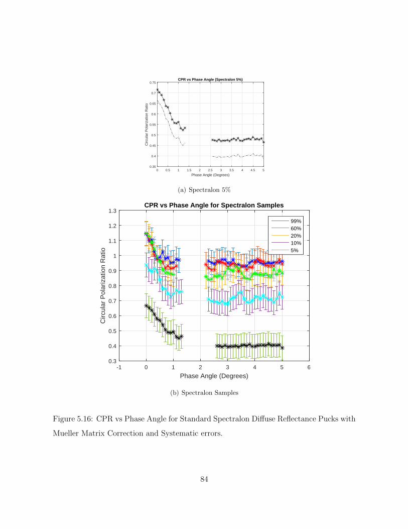
Phase Angle (Degrees)0 0.5 1 1.5 2 2.5 3 3.5 4 4.5 5
Circ
ular
Pol
ariz
atio
n R
atio
0.35
0.4
0.45
0.5
0.55
0.6
0.65
0.7
0.75CPR vs Phase Angle (Spectralon 5%)
(a) Spectralon 5%
Phase Angle (Degrees)-1 0 1 2 3 4 5 6
Circ
ular
Pol
ariz
atio
n R
atio
0.3
0.4
0.5
0.6
0.7
0.8
0.9
1
1.1
1.2
1.3CPR vs Phase Angle for Spectralon Samples
99%60%20%10%5%
(b) Spectralon Samples
Figure 5.16: CPR vs Phase Angle for Standard Spectralon Diffuse Reflectance Pucks with
Mueller Matrix Correction and Systematic errors.
84
Figures 5.15 and 5.16 show the CPR values for Standard Spectralon reflectance samples
before and after applying the M2 Mueller matrix correction. As the CPR value were
calculated from the S4 Stokes parameter of the backscattered signal, the relative trend
for the samples remained the same. For Spectralon samples with reflectance >20% we
observe the corrected CPR values at zero phase angle increase in magnitude while the
minimum values are much lower. For darker Spectralon samples the corrected CPR values
were much lower in comparison as their observed S4 parameters were lower in magnitude.
Figure 5.16b shows the relative CPR values for all the Spectralon samples, with higher
reflectance samples having higher polarization ratios while lower reflectance samples hav-
ing much smaller polarization ratios.
85
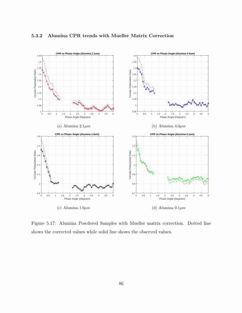
5.3.2 Alumina CPR trends with Mueller Matrix Correction
Phase Angle (Degrees)0 0.5 1 1.5 2 2.5 3 3.5 4 4.5 5
Circ
ular
Pol
ariz
atio
n R
atio
1
1.05
1.1
1.15
1.2
1.25
1.3
1.35
1.4
1.45CPR vs Phase Angle (Alumina 2.1um)
(a) Alumina 2.1µm
Phase Angle (Degrees)0 0.5 1 1.5 2 2.5 3 3.5 4 4.5 5
Circ
ular
Pol
ariz
atio
n R
atio
0.95
1
1.05
1.1
1.15
1.2
1.25
1.3
1.35
1.4CPR vs Phase Angle (Alumina 4.0um)
(b) Alumina 4.0µm
Phase Angle (Degrees)0 0.5 1 1.5 2 2.5 3 3.5 4 4.5 5
Circ
ular
Pol
ariz
atio
n R
atio
0.9
1
1.1
1.2
1.3
1.4
1.5CPR vs Phase Angle (Alumina 1.0um)
(c) Alumina 1.0µm
Phase Angle (Degrees)0 0.5 1 1.5 2 2.5 3 3.5 4 4.5 5
Circ
ular
Pol
ariz
atio
n R
atio
0.7
0.8
0.9
1
1.1
1.2
1.3CPR vs Phase Angle (Alumina 0.1um)
(d) Alumina 0.1µm
Figure 5.17: Alumina Powdered Samples with Mueller matrix correction. Dotted line
shows the corrected values while solid line shows the observed values.
86
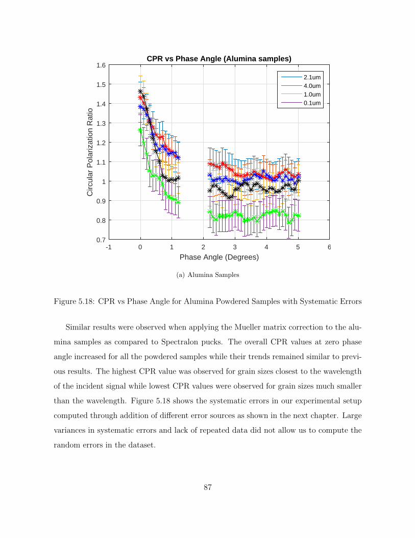
Phase Angle (Degrees)-1 0 1 2 3 4 5 6
Circ
ular
Pol
ariz
atio
n R
atio
0.7
0.8
0.9
1
1.1
1.2
1.3
1.4
1.5
1.6CPR vs Phase Angle (Alumina samples)
2.1um4.0um1.0um0.1um
(a) Alumina Samples
Figure 5.18: CPR vs Phase Angle for Alumina Powdered Samples with Systematic Errors
Similar results were observed when applying the Mueller matrix correction to the alu-
mina samples as compared to Spectralon pucks. The overall CPR values at zero phase
angle increased for all the powdered samples while their trends remained similar to previ-
ous results. The highest CPR value was observed for grain sizes closest to the wavelength
of the incident signal while lowest CPR values were observed for grain sizes much smaller
than the wavelength. Figure 5.18 shows the systematic errors in our experimental setup
computed through addition of different error sources as shown in the next chapter. Large
variances in systematic errors and lack of repeated data did not allow us to compute the
random errors in the dataset.
87

6 Error Sources and Mitigation
Mitigating the error sources are very important as they affect the data’s repeatability
and accuracy. In this chapter we shall explore the error sources encountered during the
experimental setup and the data acquisition process, the mitigation techniques employed
for these error sources will also be discussed.
6.1 Instrumentation Error
In this section we shall discuss the instrumentation challenges encountered while assem-
bling the optical system on the Goniometer and various mitigation techniques applied to
propagate these error sources. Instrumentation errors are often encountered when initially
setting up the instrument and can cause systematic and random errors in the measure-
ments, if not correctly mitigated. Here are some of the common instrumentation errors
encountered during this experiment:
88
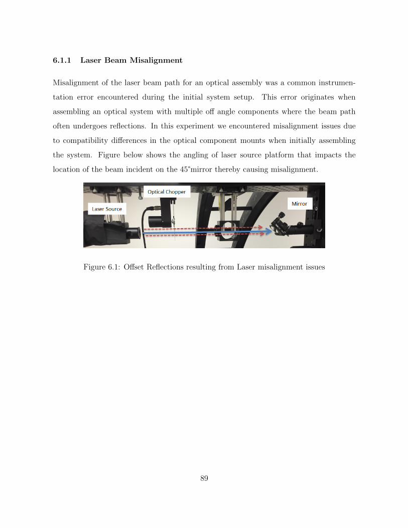
6.1.1 Laser Beam Misalignment
Misalignment of the laser beam path for an optical assembly was a common instrumen-
tation error encountered during the initial system setup. This error originates when
assembling an optical system with multiple off angle components where the beam path
often undergoes reflections. In this experiment we encountered misalignment issues due
to compatibility differences in the optical component mounts when initially assembling
the system. Figure below shows the angling of laser source platform that impacts the
location of the beam incident on the 45°mirror thereby causing misalignment.
Figure 6.1: Offset Reflections resulting from Laser misalignment issues
89
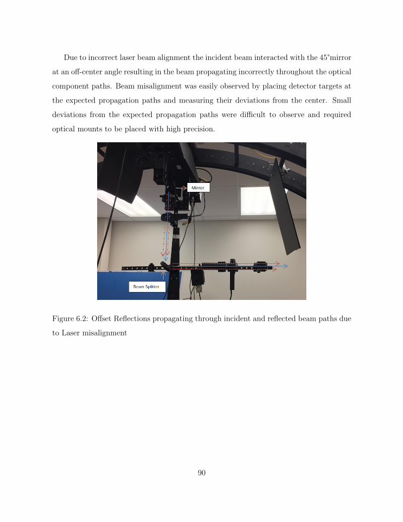
Due to incorrect laser beam alignment the incident beam interacted with the 45°mirror
at an off-center angle resulting in the beam propagating incorrectly throughout the optical
component paths. Beam misalignment was easily observed by placing detector targets at
the expected propagation paths and measuring their deviations from the center. Small
deviations from the expected propagation paths were difficult to observe and required
optical mounts to be placed with high precision.
Figure 6.2: Offset Reflections propagating through incident and reflected beam paths due
to Laser misalignment
90
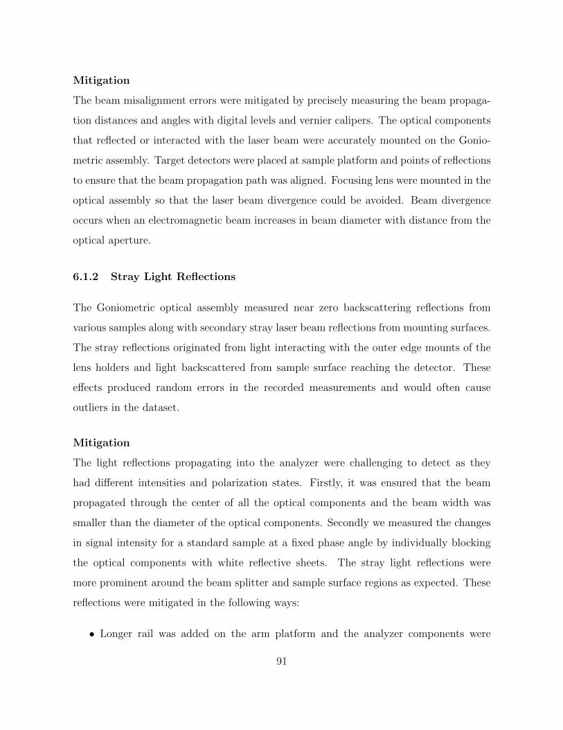
Mitigation
The beam misalignment errors were mitigated by precisely measuring the beam propaga-
tion distances and angles with digital levels and vernier calipers. The optical components
that reflected or interacted with the laser beam were accurately mounted on the Gonio-
metric assembly. Target detectors were placed at sample platform and points of reflections
to ensure that the beam propagation path was aligned. Focusing lens were mounted in the
optical assembly so that the laser beam divergence could be avoided. Beam divergence
occurs when an electromagnetic beam increases in beam diameter with distance from the
optical aperture.
6.1.2 Stray Light Reflections
The Goniometric optical assembly measured near zero backscattering reflections from
various samples along with secondary stray laser beam reflections from mounting surfaces.
The stray reflections originated from light interacting with the outer edge mounts of the
lens holders and light backscattered from sample surface reaching the detector. These
effects produced random errors in the recorded measurements and would often cause
outliers in the dataset.
Mitigation
The light reflections propagating into the analyzer were challenging to detect as they
had different intensities and polarization states. Firstly, it was ensured that the beam
propagated through the center of all the optical components and the beam width was
smaller than the diameter of the optical components. Secondly we measured the changes
in signal intensity for a standard sample at a fixed phase angle by individually blocking
the optical components with white reflective sheets. The stray light reflections were
more prominent around the beam splitter and sample surface regions as expected. These
reflections were mitigated in the following ways:
• Longer rail was added on the arm platform and the analyzer components were
91
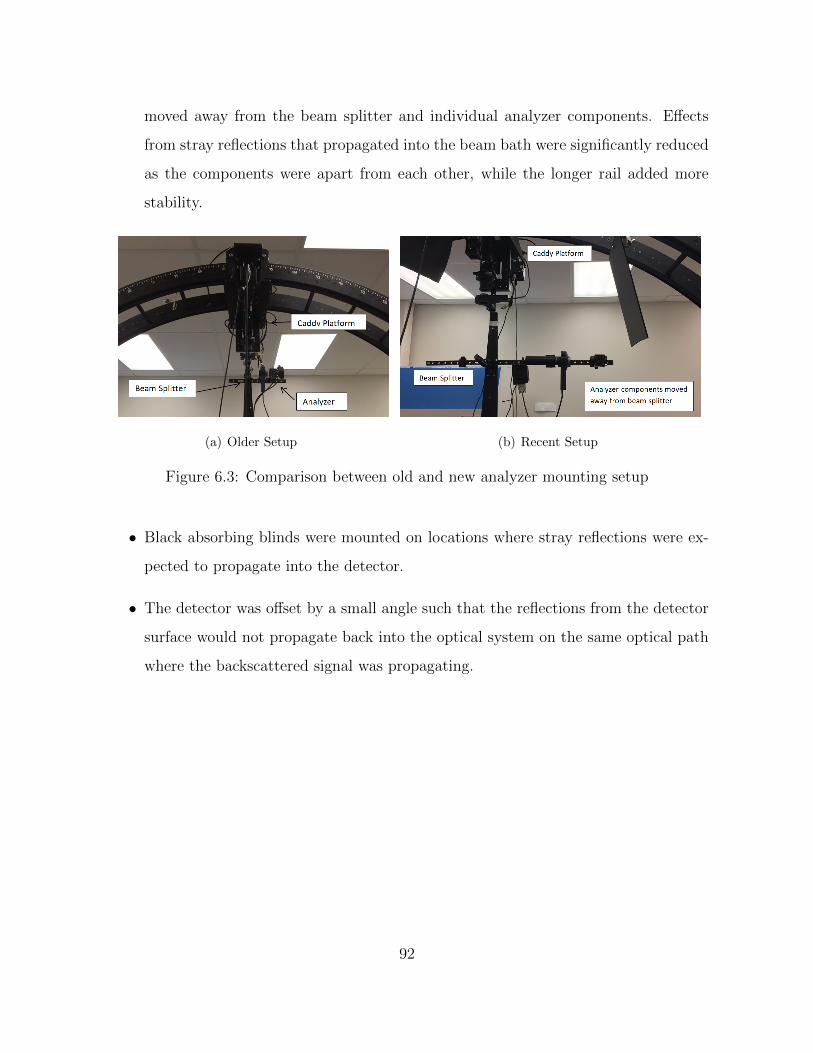
moved away from the beam splitter and individual analyzer components. Effects
from stray reflections that propagated into the beam bath were significantly reduced
as the components were apart from each other, while the longer rail added more
stability.
(a) Older Setup (b) Recent Setup
Figure 6.3: Comparison between old and new analyzer mounting setup
• Black absorbing blinds were mounted on locations where stray reflections were ex-
pected to propagate into the detector.
• The detector was offset by a small angle such that the reflections from the detector
surface would not propagate back into the optical system on the same optical path
where the backscattered signal was propagating.
92
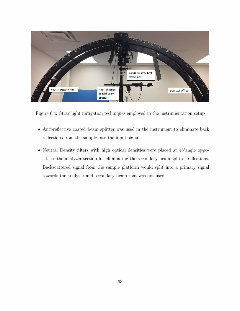
Figure 6.4: Stray light mitigation techniques employed in the instrumentation setup
• Anti-reflective coated beam splitter was used in the instrument to eliminate back
reflections from the sample into the input signal.
• Neutral Density filters with high optical densities were placed at 45°angle oppo-
site to the analyzer section for eliminating the secondary beam splitter reflections.
Backscattered signal from the sample platform would split into a primary signal
towards the analyzer and secondary beam that was not used.
93
6.1.3 Backscattering Losses
Spectralon Reflectivity (%)0 10 20 30 40 50 60 70 80 90 100
Nor
mal
ized
Sto
kes
Par
amet
er (
S0)
0
5
10
15
20
25
30
35
40
45
50Normalized Stokes Intensity (S0) vs Spectralon Reflectivity
MirrorOld Beam SplitterOutside Old Beam SplitterNew Beam Splitter
Figure 6.5: Backscattering Intensities for different reflectors with standard sample pucks
The optical component (beam splitter) that collected the backscattered radiation from
the sample source and directed it towards the analyzer lost some of the diffused signal upon
reflection. The normalized intensity Stokes parameter (S0) of standard spectralon pucks
(99% and 2%) were measured for different optical components and plotted vs spectralon
reflectivity (R). The older beam splitter had higher backscattering losses compared to the
newer beam splitter due to presence of small dust specks and absence of anti-reflective
coating. The beam splitter split the beam 50-50 twice, firstly upon incidence and secondly
when reflecting the diffused signal towards the analyzer. Due to the inaccurate S and P
polarization propagation through the beam splitter, large inaccuracies in the polarization
states were encountered for the diffuse signals.
R99%
R2%
=99
2= 49.5
The spectral reflectivity for both the 99% and 2% pucks were observed when the
94

diffused radiation were reflected from different optical components. As shown in figure
6.5, the mirror had the highest spectral reflectivity ratio of 45.13 while the beam splitters
had relatively low reflectivity ratios. The relatively low spectral reflectivity for beam
splitters could not be corrected however by measuring the Mueller matrices of the beam
splitter, the S and P polarization inaccuracies were mitigated.
95
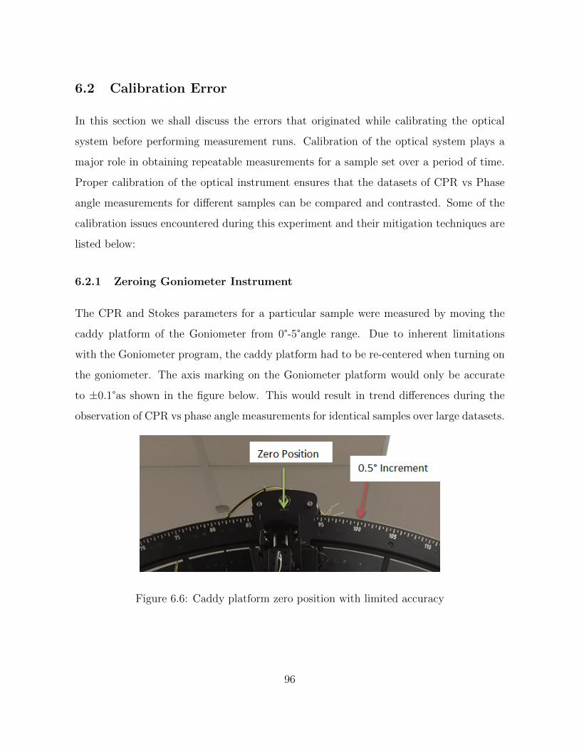
6.2 Calibration Error
In this section we shall discuss the errors that originated while calibrating the optical
system before performing measurement runs. Calibration of the optical system plays a
major role in obtaining repeatable measurements for a sample set over a period of time.
Proper calibration of the optical instrument ensures that the datasets of CPR vs Phase
angle measurements for different samples can be compared and contrasted. Some of the
calibration issues encountered during this experiment and their mitigation techniques are
listed below:
6.2.1 Zeroing Goniometer Instrument
The CPR and Stokes parameters for a particular sample were measured by moving the
caddy platform of the Goniometer from 0°-5°angle range. Due to inherent limitations
with the Goniometer program, the caddy platform had to be re-centered when turning on
the goniometer. The axis marking on the Goniometer platform would only be accurate
to ±0.1°as shown in the figure below. This would result in trend differences during the
observation of CPR vs phase angle measurements for identical samples over large datasets.
Figure 6.6: Caddy platform zero position with limited accuracy
96

Mitigation
The accuracy for caddy platform positioning was improved by measuring the axial tilt
of the platform with respect to the sample platform by a digital level. By aligning both
the platform values and centering the incident beam on the sample platform the zeroing
issues were mitigated. The successive caddy calibrations were positioned to the measured
level zero reading before all the measurements were performed.
97
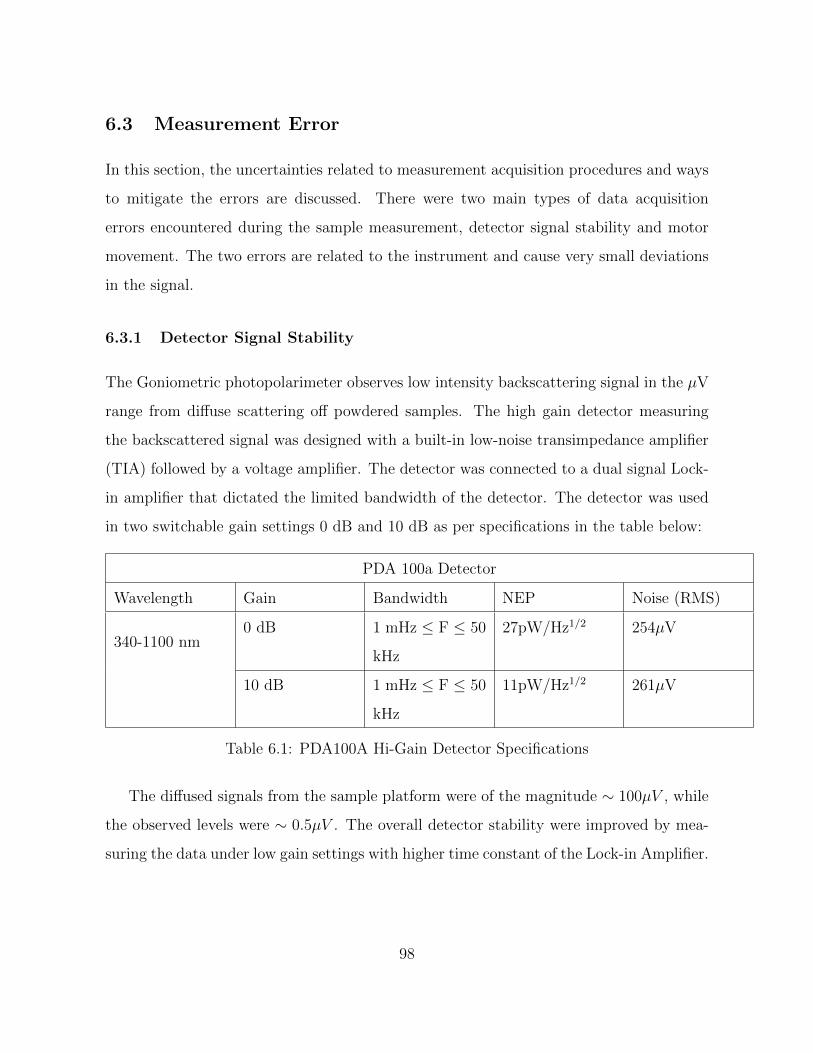
6.3 Measurement Error
In this section, the uncertainties related to measurement acquisition procedures and ways
to mitigate the errors are discussed. There were two main types of data acquisition
errors encountered during the sample measurement, detector signal stability and motor
movement. The two errors are related to the instrument and cause very small deviations
in the signal.
6.3.1 Detector Signal Stability
The Goniometric photopolarimeter observes low intensity backscattering signal in the µV
range from diffuse scattering off powdered samples. The high gain detector measuring
the backscattered signal was designed with a built-in low-noise transimpedance amplifier
(TIA) followed by a voltage amplifier. The detector was connected to a dual signal Lock-
in amplifier that dictated the limited bandwidth of the detector. The detector was used
in two switchable gain settings 0 dB and 10 dB as per specifications in the table below:
PDA 100a Detector
Wavelength Gain Bandwidth NEP Noise (RMS)
340-1100 nm0 dB 1 mHz ≤ F ≤ 50
kHz
27pW/Hz1/2 254µV
10 dB 1 mHz ≤ F ≤ 50
kHz
11pW/Hz1/2 261µV
Table 6.1: PDA100A Hi-Gain Detector Specifications
The diffused signals from the sample platform were of the magnitude ∼ 100µV , while
the observed levels were ∼ 0.5µV . The overall detector stability were improved by mea-
suring the data under low gain settings with higher time constant of the Lock-in Amplifier.
98
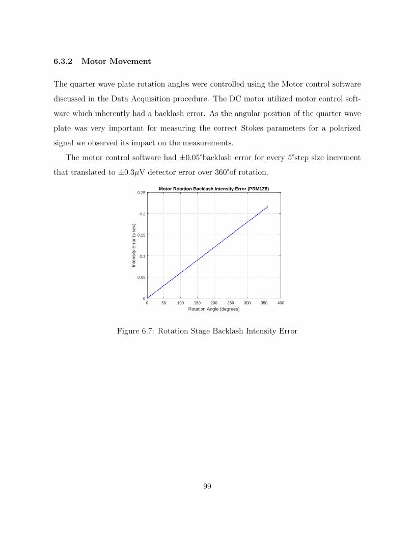
6.3.2 Motor Movement
The quarter wave plate rotation angles were controlled using the Motor control software
discussed in the Data Acquisition procedure. The DC motor utilized motor control soft-
ware which inherently had a backlash error. As the angular position of the quarter wave
plate was very important for measuring the correct Stokes parameters for a polarized
signal we observed its impact on the measurements.
The motor control software had ±0.05°backlash error for every 5°step size increment
that translated to ±0.3µV detector error over 360°of rotation.
Rotation Angle (degrees)0 50 100 150 200 250 300 350 400
Inte
nsity
Err
or (µ
sec)
0
0.05
0.1
0.15
0.2
0.25Motor Rotation Backlash Intensity Error (PRM1Z8)
Figure 6.7: Rotation Stage Backlash Intensity Error
99
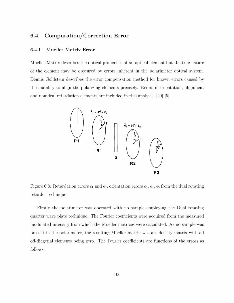
6.4 Computation/Correction Error
6.4.1 Mueller Matrix Error
Mueller Matrix describes the optical properties of an optical element but the true nature
of the element may be obscured by errors inherent in the polarimeter optical system.
Dennis Goldstein describes the error compensation method for known errors caused by
the inability to align the polarizing elements precisely. Errors in orientation, alignment
and nonideal retardation elements are included in this analysis. [20] [5]
Figure 6.8: Retardation errors ε1 and ε2, orientation errors ε3, ε4, ε5 from the dual rotating
retarder technique
Firstly the polarimeter was operated with no sample employing the Dual rotating
quarter wave plate technique. The Fourier coefficients were acquired from the measured
modulated intensity from which the Mueller matrices were calculated. As no sample was
present in the polarimeter, the resulting Mueller matrix was an identity matrix with all
off-diagonal elements being zero. The Fourier coefficients are functions of the errors as
follows:
100
a0 =1
4+
(1− ε1)(1− ε2)16
a2 =(1 + ε1)(1− ε2)
16+
(1 + ε1)(1− ε2)ε3ε52
a8 =(1 + ε1)(1 + ε2)
16
a10 =(1− ε1)(1 + ε2)
16
b2 = −(1 + ε1)(1− ε2)ε34
+(1 + ε1)(1− ε2)ε5
8
b4 =(ε4 − ε3 − ε5)
4
b6 =(ε5 − ε3 − ε4)
4
b8 =(1 + ε1)(1 + ε2)(2ε4 − 2ε3 − ε5)
8
b10 = −(1− ε1)(1 + ε2)(2ε4 − ε5)8
The above equations were inverted to solve for the errors in terms of Fourier coefficients
with no sample measurement.
ε1 = 3− 8(a0 + a10)
ε2 =4(a0 − a10)− 1
1− 4(a0 − a10)
ε3 = −2(b4 + b6)
101
ε5 =8b2
(1 + ε1)1− ε2)+ 2ε3
ε4 = ε5 + 2(b4 − b6)
Secondly, using the error-compensation equations and the known Fourier coefficients
from no sample measurement the values for errors in the polarimeter were calculated.
Lastly the systematic errors in the Fourier coefficients arising from imperfections are
compensated by using the error-compensated equations with experimentally determined
error values to obtain the error compensated sample Mueller matrix elements as a function
of measured Fourier coefficients.
Systematic Errors
Error Value
ε1 -1.26°
ε2 -1°
ε3 0.17°
ε4 -0.32°
ε5 -0.26°
Table 6.2: Alignment Errors from Mueller matrix calibration
Table 6.2 shows that ε1 and ε2 errors associated with the retardance of the quarter
wave plate are the main sources of error in calculating Muller matrices. Other orientation
error components such as quarter wave plate misalignment relative to measurement axis
and polarizer misalignment are relatively smaller in magnitude.
102
6.4.2 True Retardance Error
The true retardance of the rotating quarter wave plate was calculated by using the cross-
polarized method. The fast axis of the quarter wave plate was aligned to 45°and placed
after the linear polarizer to generate RHCP or LHCP. Misalignment or inherent errors
in the quarter wave plate would skew the circular polarization into elliptical polarization
if the true retardance was not known. Using the cross-polarized method suggested by
Goldstein, the quarter wave plate was inserted between two crossed linear polarizers. From
the markings on the quarter wave plate the fast axis was moved 45°on either clockwise or
counter-clockwise direction. When the angle between the fast axis of the wave plate and
the X-direction is at 45°, the intensity after the analyzer can be expressed as a function
of the retardance δ of the wave plate and angle α of the analyzer transmission axis with
the x direction:
I(α, δ) =I04
(1 + cos(δ)cos(2α))
Measuring the intensity at 0°and 90°angle of analyzing polarizer the true retardance
can be calculated as:
cos(δ) =I(0, δ)− I(90, δ)
I(0, δ) + I(90, δ)
The primary advantage with the cross-polarized method was that it was independent
of the source intensity. Using high precision rotation mounts for the linear polarizer and
quarter wave plate allowed for precise measurements.
103
6.4.3 Least Squares Estimate
Due to the limitation in our experimental setup we were unable to acquire data between
the intervals of 1.3°-2.2° phase angles. Using the method of least squares we interpolated
a fit for the signal intensity and CPR phase curve. The fitted least squares approximation
were interpolated from existing values before and after the missing dataset region. Using
the least squares approximation we acquired very close approximations to what is expected
in the missing regions.
Least squares interpolation was applied from five measurement before and after the
missing phase angle region. The Matlab software implements a 1D interpolation function
as shown below [26]:
y = interp1(x,m, xq,method, extrapolation)
Where y are the interpolated values, x are the data points, m are the missing values
and method specifies the interpolation technique, in this case a 5th order polynomial was
used to fit the phase curve.
y = a0 + a1x+ a2x2 + a3x
3 + a4x4 + a5x
5
The missing coefficient values for a0..a5 were calculated such that the sum of squares
of the deviations were minimum,
R =N∑1
(yi − (a0 + a1xi + a2x2i + a3x
3i + a4x
4i + a5x
5i ))
2
104
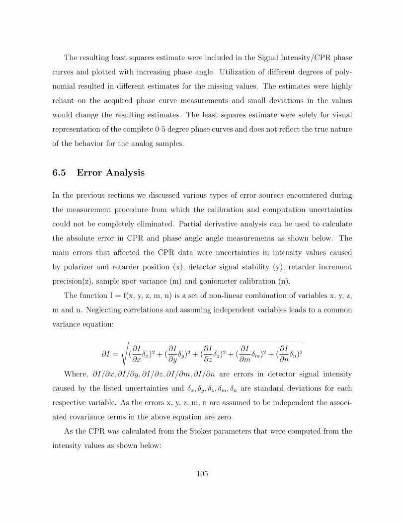
The resulting least squares estimate were included in the Signal Intensity/CPR phase
curves and plotted with increasing phase angle. Utilization of different degrees of poly-
nomial resulted in different estimates for the missing values. The estimates were highly
reliant on the acquired phase curve measurements and small deviations in the values
would change the resulting estimates. The least squares estimate were solely for visual
representation of the complete 0-5 degree phase curves and does not reflect the true nature
of the behavior for the analog samples.
6.5 Error Analysis
In the previous sections we discussed various types of error sources encountered during
the measurement procedure from which the calibration and computation uncertainties
could not be completely eliminated. Partial derivative analysis can be used to calculate
the absolute error in CPR and phase angle angle measurements as shown below. The
main errors that affected the CPR data were uncertainties in intensity values caused
by polarizer and retarder position (x), detector signal stability (y), retarder increment
precision(z), sample spot variance (m) and goniometer calibration (n).
The function I = f(x, y, z, m, n) is a set of non-linear combination of variables x, y, z,
m and n. Neglecting correlations and assuming independent variables leads to a common
variance equation:
∂I =
√(∂I
∂xδx)2 + (
∂I
∂yδy)2 + (
∂I
∂zδz)2 + (
∂I
∂mδm)2 + (
∂I
∂nδn)2
Where, ∂I/∂x, ∂I/∂y, ∂I/∂z, ∂I/∂m, ∂I/∂n are errors in detector signal intensity
caused by the listed uncertainties and δx, δy, δz, δm, δn are standard deviations for each
respective variable. As the errors x, y, z, m, n are assumed to be independent the associ-
ated covariance terms in the above equation are zero.
As the CPR was calculated from the Stokes parameters that were computed from the
intensity values as shown below:
105
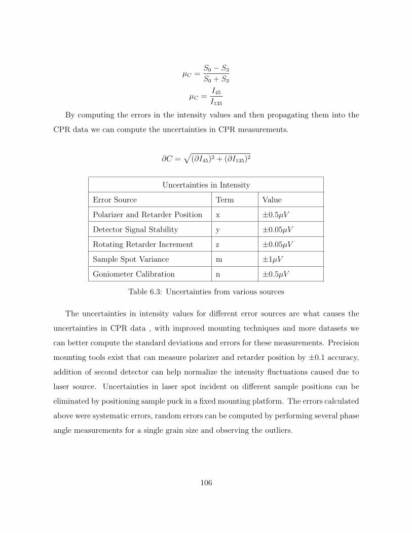
µC =S0 − S3
S0 + S3
µC =I45I135
By computing the errors in the intensity values and then propagating them into the
CPR data we can compute the uncertainties in CPR measurements.
∂C =√
(∂I45)2 + (∂I135)2
Uncertainties in Intensity
Error Source Term Value
Polarizer and Retarder Position x ±0.5µV
Detector Signal Stability y ±0.05µV
Rotating Retarder Increment z ±0.05µV
Sample Spot Variance m ±1µV
Goniometer Calibration n ±0.5µV
Table 6.3: Uncertainties from various sources
The uncertainties in intensity values for different error sources are what causes the
uncertainties in CPR data , with improved mounting techniques and more datasets we
can better compute the standard deviations and errors for these measurements. Precision
mounting tools exist that can measure polarizer and retarder position by ±0.1 accuracy,
addition of second detector can help normalize the intensity fluctuations caused due to
laser source. Uncertainties in laser spot incident on different sample positions can be
eliminated by positioning sample puck in a fixed mounting platform. The errors calculated
above were systematic errors, random errors can be computed by performing several phase
angle measurements for a single grain size and observing the outliers.
106
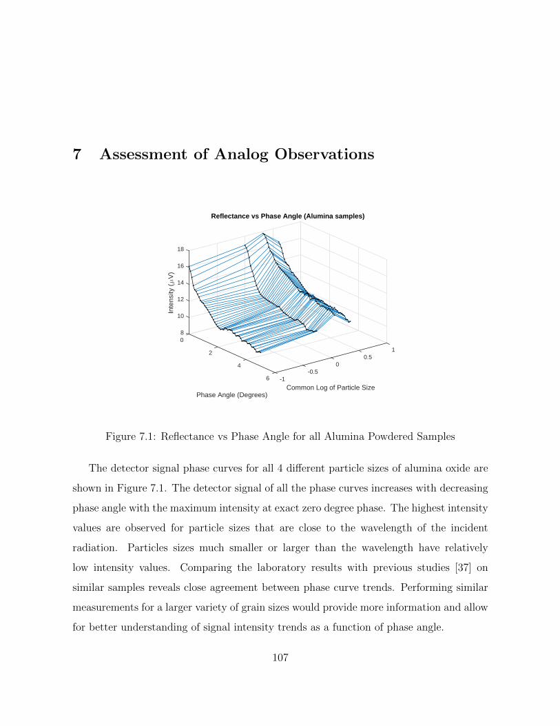
7 Assessment of Analog Observations
1
Common Log of Particle Size
0.5
Reflectance vs Phase Angle (Alumina samples)
0-0.5
-16
Phase Angle (Degrees)
4
2
12
14
16
18
10
80
Inte
nsity
(µ
V)
Figure 7.1: Reflectance vs Phase Angle for all Alumina Powdered Samples
The detector signal phase curves for all 4 different particle sizes of alumina oxide are
shown in Figure 7.1. The detector signal of all the phase curves increases with decreasing
phase angle with the maximum intensity at exact zero degree phase. The highest intensity
values are observed for particle sizes that are close to the wavelength of the incident
radiation. Particles sizes much smaller or larger than the wavelength have relatively
low intensity values. Comparing the laboratory results with previous studies [37] on
similar samples reveals close agreement between phase curve trends. Performing similar
measurements for a larger variety of grain sizes would provide more information and allow
for better understanding of signal intensity trends as a function of phase angle.
107
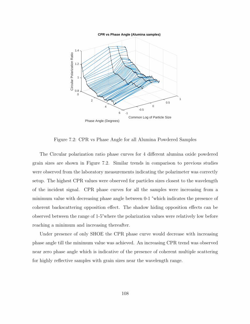
1
Common Log of Particle Size
0.5
CPR vs Phase Angle (Alumina samples)
0-0.5
-16
Phase Angle (Degrees)
4
2
1.4
0.8
1
1.2
0
Circ
ular
Pol
ariz
atio
n R
atio
Figure 7.2: CPR vs Phase Angle for all Alumina Powdered Samples
The Circular polarization ratio phase curves for 4 different alumina oxide powdered
grain sizes are shown in Figure 7.2. Similar trends in comparison to previous studies
were observed from the laboratory measurements indicating the polarimeter was correctly
setup. The highest CPR values were observed for particles sizes closest to the wavelength
of the incident signal. CPR phase curves for all the samples were increasing from a
minimum value with decreasing phase angle between 0-1 °which indicates the presence of
coherent backscattering opposition effect. The shadow hiding opposition effects can be
observed between the range of 1-5°where the polarization values were relatively low before
reaching a minimum and increasing thereafter.
Under presence of only SHOE the CPR phase curve would decrease with increasing
phase angle till the minimum value was achieved. An increasing CPR trend was observed
near zero phase angle which is indicative of the presence of coherent multiple scattering
for highly reflective samples with grain sizes near the wavelength range.
108
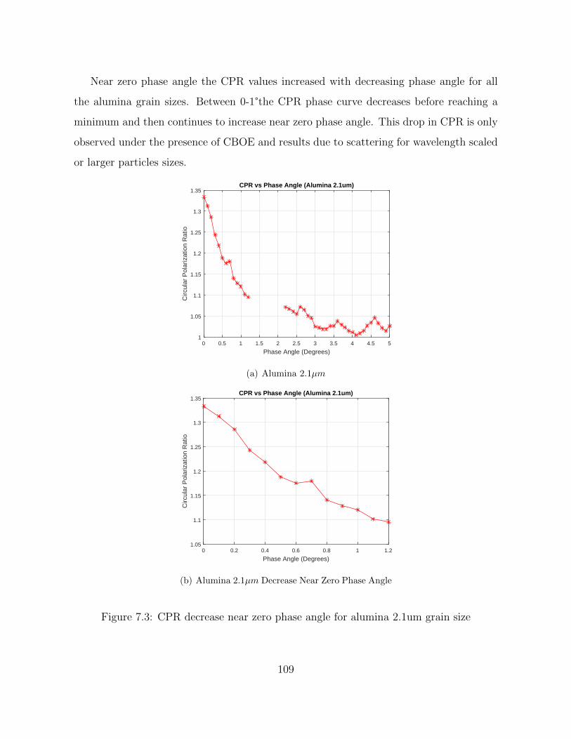
Near zero phase angle the CPR values increased with decreasing phase angle for all
the alumina grain sizes. Between 0-1°the CPR phase curve decreases before reaching a
minimum and then continues to increase near zero phase angle. This drop in CPR is only
observed under the presence of CBOE and results due to scattering for wavelength scaled
or larger particles sizes.
Phase Angle (Degrees)0 0.5 1 1.5 2 2.5 3 3.5 4 4.5 5
Circ
ular
Pol
ariz
atio
n R
atio
1
1.05
1.1
1.15
1.2
1.25
1.3
1.35CPR vs Phase Angle (Alumina 2.1um)
(a) Alumina 2.1µm
Phase Angle (Degrees)0 0.2 0.4 0.6 0.8 1 1.2
Circ
ular
Pol
ariz
atio
n R
atio
1.05
1.1
1.15
1.2
1.25
1.3
1.35CPR vs Phase Angle (Alumina 2.1um)
(b) Alumina 2.1µm Decrease Near Zero Phase Angle
Figure 7.3: CPR decrease near zero phase angle for alumina 2.1um grain size
109
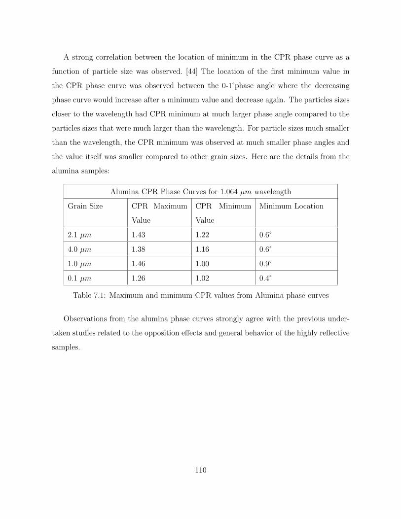
A strong correlation between the location of minimum in the CPR phase curve as a
function of particle size was observed. [44] The location of the first minimum value in
the CPR phase curve was observed between the 0-1°phase angle where the decreasing
phase curve would increase after a minimum value and decrease again. The particles sizes
closer to the wavelength had CPR minimum at much larger phase angle compared to the
particles sizes that were much larger than the wavelength. For particle sizes much smaller
than the wavelength, the CPR minimum was observed at much smaller phase angles and
the value itself was smaller compared to other grain sizes. Here are the details from the
alumina samples:
Alumina CPR Phase Curves for 1.064 µm wavelength
Grain Size CPR Maximum
Value
CPR Minimum
Value
Minimum Location
2.1 µm 1.43 1.22 0.6°
4.0 µm 1.38 1.16 0.6°
1.0 µm 1.46 1.00 0.9°
0.1 µm 1.26 1.02 0.4°
Table 7.1: Maximum and minimum CPR values from Alumina phase curves
Observations from the alumina phase curves strongly agree with the previous under-
taken studies related to the opposition effects and general behavior of the highly reflective
samples.
110
8 Conclusion
The aim of this thesis has been to firstly design and construct an optical polarimeter
capable of measuring polarization state of backscattered signal from analog samples and
secondly to observe the properties of the analog samples and infer important information
regarding the backscattering properties for highly reflective wavelength-scaled particles.
Chapter 2 provided a theoretical background related to the polarization state of an
electromagnetic signal and important parameters that can be acquired from the polarized
phase curves. Chapter 3 explored the different techniques through which the polariza-
tion state of a signal can be acquired and changed by optical components. Chapter 4
demonstrated the measurement procedure and optical setup employed on the long arm
goniometric instrument for measuring polarized backscatter signal. Using the polarimet-
ric instrument several analog measurements from different samples were acquired and
corrected for polarization changes as listed in chapter 5. Errors associated with the in-
strumentation, calibration, measurement and computation are listed and mitigated in the
error sources and mitigation section. The research objectives for this study were intended
to guide the construction of the polarimetric setup and deduce important information
related to the analog samples from the polarized backscattered signal.
The primary objective of the undertaken research was addressed by designing and
assembling an experimental setup capable of measuring detector signal and Stokes vector
for a backscattering signal over 0-5 degree phase angles. The detector signal and polar-
ization measurements allowed us to calculate circular polarization ratio through which we
observed the presence of opposition effects near zero phase angle. Coherent backscatter-
ing opposition effects were observed for all the highly reflective alumina grain sizes along
111
with the standard spectralon samples. From the near zero opposition surge we observed
the dependence of the wavelength and particle size on the coherent backscattering trends.
For our second research objective, a rotating quarter wave plate technique was em-
ployed on the goniometeric instrument that was capable of measuring Stokes vector of
a backscattered wave. By using different orientations of the linear polarizer and quarter
wave plate with precision mounts we were able to provide highly polarized right and left
circular incident signal on the sample platform for measuring the resulting backscatter.
The Stokes vector of the backscattered signal provided important information regarding
the polarization state of the wave with high accuracy.
For achieving the instrument capability of performing backscatter measurements over
0-5 degree range ,we employed a beam splitter that allowed for exact zero phase an-
gle measurements. Due to mounting limitations phase angles from 1.3-2.2°could not be
successfully acquired. Future work on eliminating mounting restrictions will allow us
to measure seamless backscatter data from 0-5 degree phase. Uncertainties occurring
through uneven beam-splitter reflections into the analyzer affected the polarization state
of the measured data. To eliminate this uncertainty, Mueller matrices for the reflecting
optical component were acquired and applied to the Stokes vector of the measured signal
to eliminate the polarization change from the beam splitter.
From the acquired Stokes vector over a 5 degree phase range, important parameters
such as the circular polarization ratio and linear polarization ratio were calculated. The
detector signal phase curves indicated the presence of opposition surge as the backscatter
intensity increased at near zero phase angles. Further calculation of the polarization
ratios enabled us to differentiate between the two opposition effects. SHOE primarily
was a single scattering effect where the CPR was expected to decrease as the phase angle
decreased, however due to presence of CBOE the CPR values increased with decreasing
phase angle. The presence of CBOE agreed with previous undertaken studies and provided
evidence that potential highly reflective ice bearing deposits would have similar occurring
phenomenon but more future work on the liquid samples are required.
112
The fifth research objective was to explore the key variables such as size and size dis-
tribution of the scatterers, the number density of the scatterers, the absorption properties
of the medium hosting the scatterers, and the absorption properties of the scatterers
themselves. Polystyrene beads the size approximately equal to the wavelength of the
incident radiation were suspended in a milky liquid solution and the backscatter signal
were observed. Specular reflections from the initial contact of the polarized signal with
the liquid medium required us to observe the backscatter at large incidence angles. Al-
though the liquid suspension was a low-loss medium, very weak and noisy backscattering
signal was observed. The suspended beads in the liquid medium would settle through the
polarization measurement procedure which would further affect the repeatability of the
measurements. The objectives related to the size distribution of scatterers, absorption
properties of the medium and of the scatterers could not be achieved. Future work on
preparing a more stable measurement technique for liquid beads is required before the
absorption and scattering properties can be calculated.
I accomplished the primary objectives of the research by designing, constructing and
re-iterating the design of the polarimeter according to the given objectives. The instru-
ment was validated by measuring the CPR and signal intensity values over 0-5°phase angle
region and comparing those values to the Nelson (2000) [37] study. Although the Nelson
study used different wavelength compared to my study. I was able to observe similar
trends for CPR and intensity values with decreasing phase angle. The trends were also
observed for some liquid analog samples suggesting that multiple scattering effects can be
studied through this instrument. Future work involving a variety of liquid samples and
possibly icy analogs using the MAGI polarimeter would provide more evidence on the
behavior of scatters, scattering medium and nature of scatterers.
113
9 Future Work
Although the results presented here have demonstrated the capability for acquisition of
polarized backscatter at near zero phase angles and the presence of opposition effects for
highly reflective samples, it can be further improved. Future work for developing two
main aspects of the experiment; instrumentation and sample utilization will help improve
the understanding for the detection of icy regoliths.
Instrumentation
• The overall time for acquisition of a single Stokes vector for a backscattered signal
was >20 minutes, while the acquisition of CPR values over 0-5 degree phase angle
were >45 minutes. Future work to integrate and automate the Stokes vector acqui-
sition and Goniometer movement software would help reduce the data acquisition
time. This provides sufficient time to prevent the liquid suspension from settling
and allow for a stable measurement.
• Signal stability and low signal to noise ratios are believed to be the biggest con-
tributors to uncertainties in the data acquisition procedure. Measuring the stability
of the laser for a low intensity signal would help circumvent the uncertainty issues
by applying proper corrections. Acquisition of signal over different IR and visible
wavelengths would help us understand the effects of wavelength on CPR trends and
reflectance values.
114
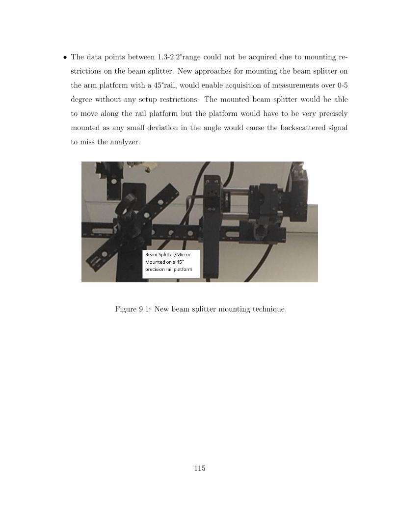
• The data points between 1.3-2.2°range could not be acquired due to mounting re-
strictions on the beam splitter. New approaches for mounting the beam splitter on
the arm platform with a 45°rail, would enable acquisition of measurements over 0-5
degree without any setup restrictions. The mounted beam splitter would be able
to move along the rail platform but the platform would have to be very precisely
mounted as any small deviation in the angle would cause the backscattered signal
to miss the analyzer.
Figure 9.1: New beam splitter mounting technique
115
Future Samples
• The phase angle measurements were performed for four different highly reflective
alumina samples with grain sizes higher, lower and similar to the wavelength of the
incident signal. Future data measurements for alumina samples with more diverse
set of grain sizes would help develop a complete phase curve map.
• The analogs used for this study were mainly powdered alumina samples and stan-
dard Spectralon pucks. To better understand the behaviour of icy regoliths, single
sample of aqueous suspension with polystyrene beads from Thermo Fisher Scientific
manufacturer [33] and Alumina (2.1µm)/Glycerol colloidal solution were studied
and analyzed at different emergence angles. Future measurements on a variety of
suspended bead solutions with different particle sizes in the range of the wavelength
of the signal would help understand the behavior of scatterers embedded in low loss
medium.
116
Bibliography
[1] Effects of interaction of electromagnetic waves in complex particles. URL: http:
//what-when-how.com/electromagnetic-waves.htm [cited 10.05.2018].
[2] Normal probability density function, 2018. URL: https://www.mathworks.com/
help/stats/normpdf.html.
[3] E. Akkermans, P. E. Wolf, and R. Maynard. Coherent backscattering of light by dis-
ordered media: Analysis of the peak line shape. Phys. Rev. Lett., 56:1471–1474, Apr
1986. URL: https://link.aps.org/doi/10.1103/PhysRevLett.56.1471, doi:
10.1103/PhysRevLett.56.1471.
[4] Von Sebastian Arnoldt. Rotating quarter-wave plate stokes polarimeter. 2011.
URL: http://quantum-technologies.iap.uni-bonn.de/en/diplom-theses.
html?task=download&file=216&token=294e84a6672a486d881880d560973c68.
[5] R. M. A. Azzam. Photopolarimetric measurement of the mueller matrix by fourier
analysis of a single detected signal. Opt. Lett., 2(6):148–150, Jun 1978. URL: http:
//ol.osa.org/abstract.cfm?URI=ol-2-6-148, doi:10.1364/OL.2.000148.
[6] D. Blewett B. Hapke. Coherent backscatter model for the unusual radar reflectivity
of icy satellites. Nature, 352:46–47, 1991. doi:10.1038/352046a0.
[7] Malvin Carl Teich Bahaa E.A. Saleh. Polarization and Crystal Optics. Wiley-
Blackwell, 2001. URL: https://onlinelibrary.wiley.com/doi/abs/10.1002/
0471213748.ch6, doi:10.1002/0471213748.ch6.
117
[8] Lance A.M. Benner, Steven J. Ostro, Christopher Magri, Michael C. Nolan,
Ellen S. Howell, Jon D. Giorgini, Raymond F. Jurgens, Jean-Luc Margot,
Patrick A. Taylor, Michael W. Busch, and Michael K. Shepard. Near-earth
asteroid surface roughness depends on compositional class. Icarus, 198(2):294
– 304, 2008. URL: http://www.sciencedirect.com/science/article/pii/
S0019103508002522, doi:https://doi.org/10.1016/j.icarus.2008.06.010.
[9] Bryan J. Butler, Duane O. Muhleman, and Martin A. Slade. Mercury: full-disk
radar images and the detection and stability of ice at the north pole. Journal of
Geophysical Research: Planets, 98(E8):15003–15023, 1993. URL: http://dx.doi.
org/10.1029/93JE01581, doi:10.1029/93JE01581.
[10] B.A. Campbell. Radar Remote Sensing of Planetary Surfaces. Cambridge University
Press, 2002.
[11] Bruce A. Campbell, Lynn M. Carter, Donald B. Campbell, Michael Nolan, John
Chandler, Rebecca R. Ghent, B. Ray Hawke, Ross F. Anderson, and Kassan-
dra Wells. Earth-based 12.6-cm wavelength radar mapping of the moon: New
views of impact melt distribution and mare physical properties. Icarus, 208(2):565
– 573, 2010. URL: http://www.sciencedirect.com/science/article/pii/
S0019103510001132, doi:https://doi.org/10.1016/j.icarus.2010.03.011.
[12] Bruce A. Campbell, B. R. Hawke, and Donald B. Campbell. Surface morphol-
ogy of domes in the marius hills and mons rumker regions of the moon from
earth-based radar data. Journal of Geophysical Research: Planets, 114(E1):n/a–
n/a, 2009. E01001. URL: http://dx.doi.org/10.1029/2008JE003253, doi:
10.1029/2008JE003253.
[13] L. M. Carter, D. B. Campbell, and B. A. Campbell. Geologic studies of planetary
surfaces using radar polarimetric imaging. Proceedings of the IEEE, 99(5):770–782,
May 2011. doi:10.1109/JPROC.2010.2099090.
118
[14] S. Chandrasekhar. Radiative Transfer. Dover Books on Physics. Dover Publications,
2013. URL: https://books.google.ca/books?id=1YHCAgAAQBAJ.
[15] Les Cowley. Shadow hiding. URL: https://www.atoptics.co.uk/fz481.htm [cited
10.05.2018].
[16] Wenzhe Fa and Yuzhen Cai. Circular polarization ratio characteristics of impact
craters from mini-rf observations and implications for ice detection at the polar re-
gions of the moon. Journal of Geophysical Research: Planets, 118(8):1582–1608,
2013. URL: http://dx.doi.org/10.1002/jgre.20110, doi:10.1002/jgre.20110.
[17] Wenzhe Fa, Mark A. Wieczorek, and Essam Heggy. Modeling polarimet-
ric radar scattering from the lunar surface: Study on the effect of physi-
cal properties of the regolith layer. Journal of Geophysical Research: Plan-
ets, 116(E3). URL: https://agupubs.onlinelibrary.wiley.com/doi/abs/10.
1029/2010JE003649, arXiv:https://agupubs.onlinelibrary.wiley.com/doi/
pdf/10.1029/2010JE003649, doi:10.1029/2010JE003649.
[18] T. Gehrels. Photometric Studies of Asteroids. V. The Light-Curve and Phase Func-
tion of 20 Massalia. Astrophysics Journal, 123:331, March 1956. doi:10.1086/
146166.
[19] Rebecca R. Ghent, Bruce A. Campbell, B. Ray Hawke, and Donald B. Camp-
bell. Earth-based radar data reveal extended deposits of the moon’s orientale
basin. Geology, 36(5):343, 2008. URL: +http://dx.doi.org/10.1130/G24325A.
1, arXiv:/gsw/content_public/journal/geology/36/5/10.1130_g24325a.1/3/
i0091-7613-36-5-343.pdf, doi:10.1130/G24325A.1.
[20] Dennis H. Goldstein. Mueller matrix dual-rotating retarder polarimeter. Appl.
Opt., 31(31):6676–6683, Nov 1992. URL: http://ao.osa.org/abstract.cfm?URI=
ao-31-31-6676, doi:10.1364/AO.31.006676.
119
[21] K. A. Hameen-Anttila and S. Pyykko. Photometric Behaviour of Saturn’s Rings as
a Function of the Saturn ocentric Latitudes of the Earth and the Sun. Astronomy
and Astrophysics, 19:235, July 1972.
[22] B. Hapke, D. Dimucci, R. Nelson, and W. Smythe. The Nature of the Opposition
Effect in Frost, Vegetation and Soils. In Lunar and Planetary Science Conference,
volume 27 of Lunar and Planetary Science Conference, March 1996.
[23] Bruce Hapke. Coherent backscatter and the radar characteristics of outer planet
satellites. Icarus, 88(2):407 – 417, 1990. URL: http://www.sciencedirect.
com/science/article/pii/001910359090091M, doi:https://doi.org/10.1016/
0019-1035(90)90091-M.
[24] Bruce W. Hapke, Robert M. Nelson, and William D. Smythe. The op-
position effect of the moon: The contribution of coherent backscatter.
Science, 260(5107):509–511, 1993. URL: http://science.sciencemag.org/
content/260/5107/509, arXiv:http://science.sciencemag.org/content/260/
5107/509.full.pdf, doi:10.1126/science.260.5107.509.
[25] K. Ichimoto, K. Shinoda, T. Yamamoto, and J. Kiyohara. Photopolarimetric mea-
surement system of Mueller matrix with dual rotating waveplates. Publications of
the National Astronomical Observatory of Japan, 9:11–19, 2006.
[26] Least Squares Interpolation. 1d interpolation. URL: https://www.mathworks.com/
help/matlab/ref/interp1.html#btwp6lt-1-x.
[27] M. A. Janssen, A. Le Gall, and L. C. Wye. Anomalous radar backscatter from Titan’s
surface? Icarus, 212:321–328, March 2011. doi:10.1016/j.icarus.2010.11.026.
[28] B. Jost, A. Pommerol, O. Poch, B. Gundlach, M. Leboeuf, M. Dadras,
J. Blum, and N. Thomas. Experimental characterization of the opposition
surge in fine-grained water–ice and high albedo ice analogs. Icarus, 264:109
120
– 131, 2016. URL: http://www.sciencedirect.com/science/article/pii/
S001910351500425X, doi:https://doi.org/10.1016/j.icarus.2015.09.020.
[29] Dissanska M Levesque M.P. ”measurement and modeling of the spectralon™ spectro-
polarimetric bidirectional reflectance distribution function (brdf)”, 2016.
[30] Michael Light. Opposition effects, 2002. URL: https://www.atoptics.co.uk/
atoptics/oppos1.htm [cited 10.05.2018].
[31] P. G. Lucey, G. A. Neumann, M. A. Riner, E. Mazarico, D. E. Smith, M. T. Zuber,
D. A. Paige, D. B. Bussey, J. T. Cahill, A. McGovern, P. Isaacson, L. M. Corley, M. H.
Torrence, H. J. Melosh, J. W. Head, and E. Song. The global albedo of the moon
at 1064 nm from lola. Journal of Geophysical Research: Planets, 119(7):1665–1679,
2014. 2013JE004592. URL: http://dx.doi.org/10.1002/2013JE004592, doi:10.
1002/2013JE004592.
[32] R. Magnusson. Mueller matrix ellipsometry studies of nanostructured materials:.
Linkoping Studies in Science and Technology. Dissertations. Linkoping University
Electronic Press, 2014. URL: https://books.google.ca/books?id=FoxUBQAAQBAJ.
[33] Thermo Fisher Scientific Manufactures. Microspheres. URL: https://www.
thermofisher.com/ca/en/home.html.
[34] M. I. Mishchenko. The angular width of the coherent back-scatter opposition ef-
fect: An application to icy outer planet satellites. Astrophysics and Space Sci-
ence, 194(2):327–333, Aug 1992. URL: https://doi.org/10.1007/BF00644001,
doi:10.1007/BF00644001.
[35] M.I. Mishchenko, V.K. Rosenbush, and N.N. Kiselev. Polarimetric Remote Sensing
of Solar System Objects. Akademperiodika, 2010. URL: https://books.google.
ca/books?id=yKBltAEACAAJ.
121
[36] DUANE O. MUHLEMAN, BRYAN J. BUTLER, ARIE W. GROSSMAN, and
MARTIN A. SLADE. Radar images of mars. Science, 253(5027):1508–1513,
1991. URL: http://science.sciencemag.org/content/253/5027/1508, arXiv:
http://science.sciencemag.org/content/253/5027/1508.full.pdf, doi:10.
1126/science.253.5027.1508.
[37] R.M. Nelson, B.W. Hapke, W.D. Smythe, and L.J. Spilker. The opposition ef-
fect in simulated planetary regoliths. reflectance and circular polarization ratio
change at small phase angle. Icarus, 147(2):545 – 558, 2000. URL: http://www.
sciencedirect.com/science/article/pii/S0019103500964546, doi:https://
doi.org/10.1006/icar.2000.6454.
[38] Robert M Nelson, William D Smythe, Bruce W Hapke, and Amy S Hale. Low
phase angle laboratory studies of the opposition effect: search for wavelength de-
pendence. Planetary and Space Science, 50(9):849 – 856, 2002. Space Related
Laboratory Investigation: Materials, environments a nd life. URL: http://www.
sciencedirect.com/science/article/pii/S0032063302000594, doi:https://
doi.org/10.1016/S0032-0633(02)00059-4.
[39] S. Nozette, C. L. Lichtenberg, P. Spudis, R. Bonner, W. Ort, E. Malaret,
M. Robinson, and E. M. Shoemaker. The clementine bistatic radar ex-
periment. Science, 274(5292):1495–1498, 1996. URL: http://science.
sciencemag.org/content/274/5292/1495, arXiv:http://science.sciencemag.
org/content/274/5292/1495.full.pdf, doi:10.1126/science.274.5292.1495.
[40] S. J. Ostro, D. B. Campbell, R. A. Simpson, R. S. Hudson, J. F. Chandler, K. D.
Rosema, I. I. Shapiro, E. M. Standish, R. Winkler, D. K. Yeomans, R. Velez, and
R. M. Goldstein. Europa, ganymede, and callisto: New radar results from arecibo and
goldstone. Journal of Geophysical Research: Planets, 97(E11):18227–18244, 1992.
URL: http://dx.doi.org/10.1029/92JE01992, doi:10.1029/92JE01992.
122
[41] David A. Paige, Matthew A. Siegler, John K. Harmon, Gregory A. Neumann, Er-
wan M. Mazarico, David E. Smith, Maria T. Zuber, Ellen Harju, Mona L. Delitsky,
and Sean C. Solomon. Thermal stability of volatiles in the north polar region of
mercury. Science, 339(6117):300–303, 2013. URL: http://science.sciencemag.
org/content/339/6117/300, arXiv:http://science.sciencemag.org/content/
339/6117/300.full.pdf, doi:10.1126/science.1231106.
[42] Jennifer Lynn Piatek. Size-dependent scattering properties of planetary regolith
analogs. December 2003. URL: http://d-scholarship.pitt.edu/7875/.
[43] M. R. Chipman, Bass and Optical Society of America. Handbook of optics. Number
v. 1-2 in Handbook of Optics. McGraw-Hill, 2001. URL: https://books.google.
ca/books?id=owg6AQAAIAAJ.
[44] B. W. Hapke K. S. Manatt D. O. Kroner W. D. Smythe R. M. Nelson, M.
D. Boryta. Photometric properties of candidate planetary surface regolith ma-
terials at small phase angle: Relevance to small bodies in the outer solar sys-
tem. Lunar and Planetary Science Conference, pages 2584–2585, 2015. URL:
https://www.hou.usra.edu/meetings/lpsc2015/pdf/2584.pdf.
[45] R. K. Raney, P. D. Spudis, B. Bussey, J. Crusan, J. R. Jensen, W. Marinelli, P. McK-
erracher, C. Neish, M. Palsetia, R. Schulze, H. B. Sequeira, and H. Winters. The
lunar mini-rf radars: Hybrid polarimetric architecture and initial results. Proceedings
of the IEEE, 99(5):808–823, May 2011. doi:10.1109/JPROC.2010.2084970.
[46] Matthew H. Smith. Optimization of a dual-rotating-retarder mueller matrix po-
larimeter. Appl. Opt., 41(13):2488–2493, May 2002. URL: http://ao.osa.org/
abstract.cfm?URI=ao-41-13-2488, doi:10.1364/AO.41.002488.
[47] P. D. Spudis, D. B. J. Bussey, S. M. Baloga, J. T. S. Cahill, L. S. Glaze, G. W.
Patterson, R. K. Raney, T. W. Thompson, B. J. Thomson, and E. A. Ustinov.
Evidence for water ice on the moon: Results for anomalous polar craters from the lro
123
mini-rf imaging radar. Journal of Geophysical Research: Planets, 118(10):2016–2029,
2013. URL: http://dx.doi.org/10.1002/jgre.20156, doi:10.1002/jgre.20156.
[48] N. J. S. Stacy, D. B. Campbell, and P. G. Ford. Arecibo radar mapping
of the lunar poles: A search for ice deposits. Science, 276(5318):1527–1530,
1997. URL: http://science.sciencemag.org/content/276/5318/1527, arXiv:
http://science.sciencemag.org/content/276/5318/1527.full.pdf, doi:10.
1126/science.276.5318.1527.
[49] Øyvind Svensen, Morten Kildemo, Jerome Maria, Jakob J. Stamnes, and Øyvind
Frette. Mueller matrix measurements and modeling pertaining to spectralon white
reflectance standards. Opt. Express, 20(14):15045–15053, Jul 2012. URL: http://
www.opticsexpress.org/abstract.cfm?URI=oe-20-14-15045, doi:10.1364/OE.
20.015045.
[50] A. Virkki, K. Muinonen, and A. Penttila. Circular-Polarization Ratios and Radar
Albedos: Interpretation in Terms of Near-Surface Physical Properties of Asteroids.
In Asteroids, Comets, Meteors 2012, volume 1667 of LPI Contributions, page 6064,
May 2012.
124

Appendices
125
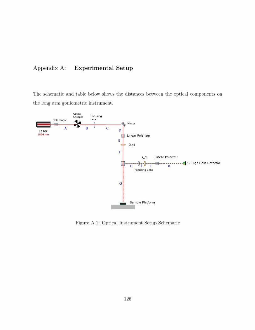
Appendix A: Experimental Setup
The schematic and table below shows the distances between the optical components on
the long arm goniometric instrument.
Figure A.1: Optical Instrument Setup Schematic
126
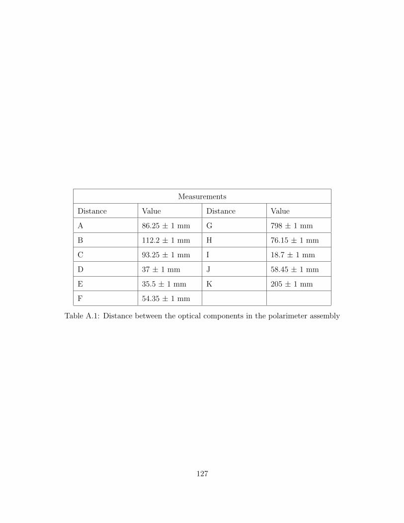
Measurements
Distance Value Distance Value
A 86.25 ± 1 mm G 798 ± 1 mm
B 112.2 ± 1 mm H 76.15 ± 1 mm
C 93.25 ± 1 mm I 18.7 ± 1 mm
D 37 ± 1 mm J 58.45 ± 1 mm
E 35.5 ± 1 mm K 205 ± 1 mm
F 54.35 ± 1 mm
Table A.1: Distance between the optical components in the polarimeter assembly
127

Appendix B: Stokes and Mueller Matrix Computation Code
The program below was written in Matlab programming language. From the experimental
rotating quarter wave plate technique the intensity values were measured in an excel
spreadsheet. The values are inserted into the program which then computes the stokes
parameters of the measured signal. Additional parameters such as same circular signal,
opposite circular signal and the circular polarization ratio are computed as well. The user
can call the program as a function every time the Stokes vector needs to be computed.
1 %% Optica l S tud i e s o f Icy Analogs us ing Near Zero Phase Angle
Measurements
2 % Stokes Parameters Computation
3 % by Mrunal Amin
4
5 %% Input the I n t e n s i t y data from Rotating Quarter Wave Plate
Technique
6 use r i npu t = input ( ’ Enter the I n t e n s i t y va lue s from RQWP
Technique :\n ’ , ’ s ’ ) ;
7 user = use r i npu t ;
8 use r input2 = input ( ’ Enter shee t number :\n ’ , ’ s ’ ) ;
9 shee t = st r2doub l e ( u s e r input2 ) ;
10 xlRange = ’B2 : B74 ’ ;
11
12 data = x l s r e ad ( user , sheet , xlRange ) ;
13
128
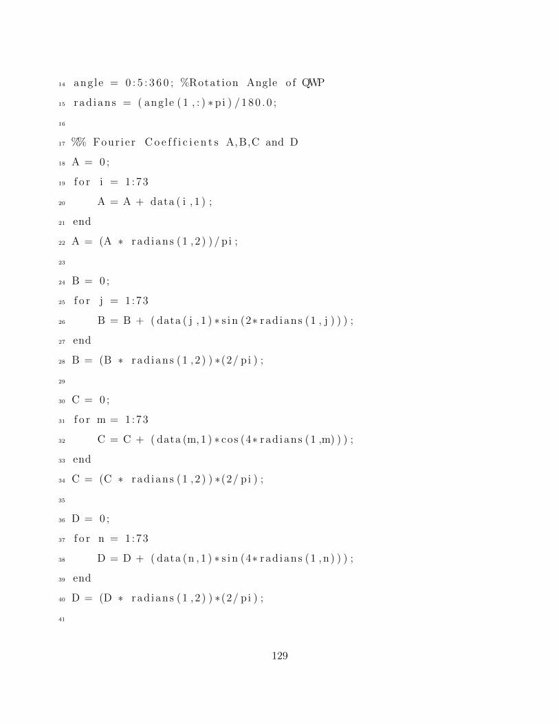
14 ang le = 0 : 5 : 3 6 0 ; %Rotation Angle o f QWP
15 rad ians = ( ang le ( 1 , : ) ∗ pi ) / 1 8 0 . 0 ;
16
17 %% Four ie r C o e f f i c i e n t s A,B,C and D
18 A = 0 ;
19 f o r i = 1 :73
20 A = A + data ( i , 1 ) ;
21 end
22 A = (A ∗ rad ians (1 , 2 ) ) / p i ;
23
24 B = 0 ;
25 f o r j = 1 :73
26 B = B + ( data ( j , 1 ) ∗ s i n (2∗ rad ians (1 , j ) ) ) ;
27 end
28 B = (B ∗ rad ians (1 , 2 ) ) ∗(2/ p i ) ;
29
30 C = 0 ;
31 f o r m = 1:73
32 C = C + ( data (m, 1 ) ∗ cos (4∗ rad ians (1 ,m) ) ) ;
33 end
34 C = (C ∗ rad ians (1 , 2 ) ) ∗(2/ p i ) ;
35
36 D = 0 ;
37 f o r n = 1:73
38 D = D + ( data (n , 1 ) ∗ s i n (4∗ rad ians (1 , n ) ) ) ;
39 end
40 D = (D ∗ rad ians (1 , 2 ) ) ∗(2/ p i ) ;
41
129
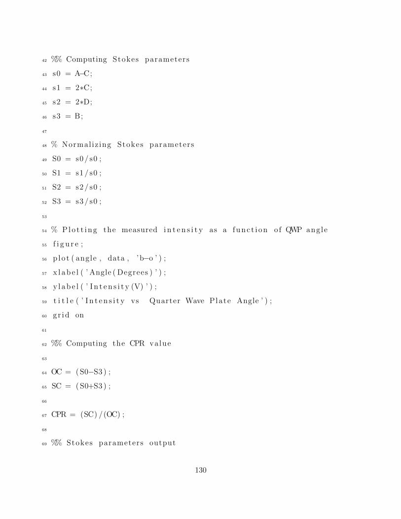
42 %% Computing Stokes parameters
43 s0 = A−C;
44 s1 = 2∗C;
45 s2 = 2∗D;
46 s3 = B;
47
48 % Normal iz ing Stokes parameters
49 S0 = s0 / s0 ;
50 S1 = s1 / s0 ;
51 S2 = s2 / s0 ;
52 S3 = s3 / s0 ;
53
54 % Plo t t i ng the measured i n t e n s i t y as a func t i on o f QWP angle
55 f i g u r e ;
56 p lo t ( angle , data , ’b−o ’ ) ;
57 x l a b e l ( ’ Angle ( Degrees ) ’ ) ;
58 y l a b e l ( ’ I n t e n s i t y (V) ’ ) ;
59 t i t l e ( ’ I n t e n s i t y vs Quarter Wave Plate Angle ’ ) ;
60 g r id on
61
62 %% Computing the CPR value
63
64 OC = ( S0−S3 ) ;
65 SC = ( S0+S3 ) ;
66
67 CPR = (SC) /(OC) ;
68
69 %% Stokes parameters output
130
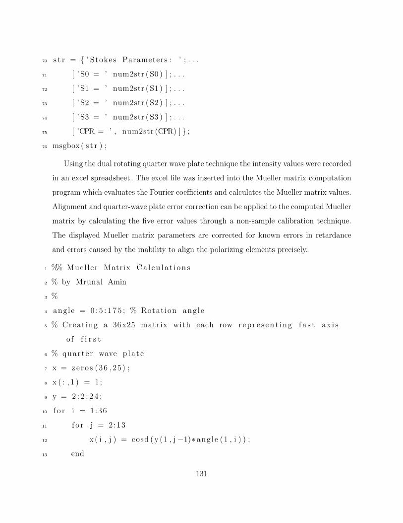
70 s t r = ’ Stokes Parameters : ’ ; . . .
71 [ ’ S0 = ’ num2str ( S0 ) ] ; . . .
72 [ ’ S1 = ’ num2str ( S1 ) ] ; . . .
73 [ ’ S2 = ’ num2str ( S2 ) ] ; . . .
74 [ ’ S3 = ’ num2str ( S3 ) ] ; . . .
75 [ ’CPR = ’ , num2str (CPR) ] ;
76 msgbox ( s t r ) ;
Using the dual rotating quarter wave plate technique the intensity values were recorded
in an excel spreadsheet. The excel file was inserted into the Mueller matrix computation
program which evaluates the Fourier coefficients and calculates the Mueller matrix values.
Alignment and quarter-wave plate error correction can be applied to the computed Mueller
matrix by calculating the five error values through a non-sample calibration technique.
The displayed Mueller matrix parameters are corrected for known errors in retardance
and errors caused by the inability to align the polarizing elements precisely.
1 %% Muel ler Matrix Ca l cu l a t i on s
2 % by Mrunal Amin
3 %
4 ang le = 0 : 5 : 1 7 5 ; % Rotation ang le
5 % Creat ing a 36x25 matrix with each row r e p r e s e n t i n g f a s t a x i s
o f f i r s t
6 % quarte r wave p l a t e
7 x = ze ro s (36 ,25) ;
8 x ( : , 1 ) = 1 ;
9 y = 2 : 2 : 2 4 ;
10 f o r i = 1 :36
11 f o r j = 2 :13
12 x ( i , j ) = cosd ( y (1 , j−1)∗ ang le (1 , i ) ) ;
13 end
131
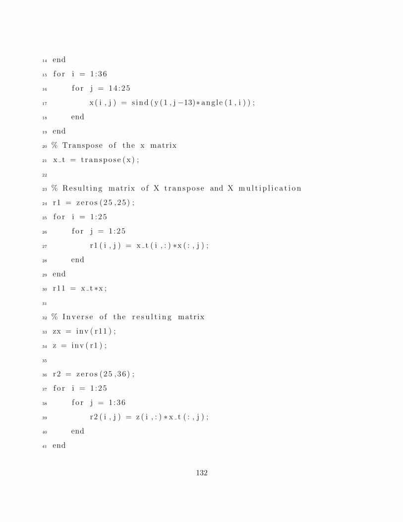
14 end
15 f o r i = 1 :36
16 f o r j = 14 :25
17 x ( i , j ) = s ind ( y (1 , j −13)∗ ang le (1 , i ) ) ;
18 end
19 end
20 % Transpose o f the x matrix
21 x t = transpose ( x ) ;
22
23 % Resu l t ing matrix o f X transpose and X m u l t i p l i c a t i o n
24 r1 = ze ro s (25 ,25) ;
25 f o r i = 1 :25
26 f o r j = 1 :25
27 r1 ( i , j ) = x t ( i , : ) ∗x ( : , j ) ;
28 end
29 end
30 r11 = x t ∗x ;
31
32 % Inve r s e o f the r e s u l t i n g matrix
33 zx = inv ( r11 ) ;
34 z = inv ( r1 ) ;
35
36 r2 = ze ro s (25 ,36) ;
37 f o r i = 1 :25
38 f o r j = 1 :36
39 r2 ( i , j ) = z ( i , : ) ∗ x t ( : , j ) ;
40 end
41 end
132

42 r22 = ( zx∗ x t ) ;
43
44 % Reading the i n t e n s i t y va lue s from the Dual Rotating Quarter
Wave
45 % Plate Method
46 use r i npu t = input ( ’ Enter the I n t e n s i t y va lue s from DRQWP
Technique :\n ’ , ’ s ’ ) ;
47 f i l ename = use r i nput ;
48 use r input2 = input ( ’ Enter shee t number :\n ’ , ’ s ’ ) ;
49 shee t = st r2doub l e ( u s e r input2 ) ; %6
50 xlRange = ’B3 : B38 ’ ;
51
52 I = x l s r e ad ( f i l ename , sheet , xlRange ) ;
53
54
55
56 %% Four ie r C o e f f i c i e n t s matrix
57 % a=ze ro s (25 ,1 ) ;
58 % f o r i = 1 :25
59 % a ( i , 1 ) = r2 ( i , : ) ∗ I ( : , 1 ) ;
60 % end
61 a = ( r22 ∗ I ) ’ ; % Simpler method compared to loop
62 %a = a ’ ;
63
64 b = ze ro s (1 , 12 ) ;
65 f o r j = 14 :25
66 b (1 , j −13) = a (1 , j ) ;
67 end
133

68
69
70 % Obtaining Muel ler components from the Four i e r C o e f f i c i e n t s
71 m11 = a (1 , 1 )−a (1 , 3 )+a (1 , 9 )−a (1 ,11 )+a (1 ,13 ) ;
72 m12 = 2∗a (1 , 3 ) − 2∗a (1 , 9 ) − 2∗a (1 ,13 ) ;
73 m13 = 2∗b (1 , 2 ) +2∗b (1 , 8 )−2∗b (1 ,12 ) ;
74 m14 = b (1 , 1 )−2∗b (1 ,11 ) ;
75 m14x = b (1 , 1 ) +2∗b (1 , 9 ) ;
76 m14x2 = b (1 , 1 )+b (1 , 9 )−b (1 ,11 ) ;
77 m21 = −2∗a (1 , 9 ) +2∗a (1 ,11 )−2∗a (1 ,13 ) ;
78 m22 = 4∗a (1 , 9 ) +4∗a (1 ,13 ) ;
79 m23 = −4∗b (1 , 8 ) +4∗b (1 ,12 ) ;
80 m24 = 2∗(−1∗b (1 , 9 )+b (1 ,11 ) ) ;
81 m24x = −4∗b (1 , 9 ) ;
82 m24x2 = 4∗b (1 ,11 ) ;
83 m31 = −2∗b (1 , 8 ) +2∗b (1 ,10 )−2∗b (1 ,12 ) ;
84 m32 = 4∗b (1 , 8 ) +4∗b (1 ,12 ) ;
85 m33 = 4∗a (1 , 9 )−4∗a (1 ,13 ) ;
86 m34 = 4∗a (1 ,10 ) ;
87 m34x = −4∗a (1 ,12 ) ;
88 m34x2 = 2∗( a (1 , 10 )−a (1 ,12 ) ) ;
89 m41 = 2∗b (1 , 3 )−b (1 , 5 ) ;
90 m41x = b (1 , 3 )−b (1 , 5 )+b (1 , 7 ) ;
91 m41x2 = −1∗b (1 , 5 ) +2∗b (1 , 7 ) ;
92 m42 = −4∗b (1 , 7 ) ;
93 m42x = −4∗b (1 , 3 ) ;
94 m42x2 = −2∗(b (1 , 3 )+b (1 , 7 ) ) ;
95 m43 = −4∗a (1 , 4 ) ;
134

96 m43x = 4∗a (1 , 8 ) ;
97 m43x2 = 2∗(−1∗a (1 , 4 )+ a (1 , 8 ) ) ;
98 m44 = −2∗a (1 , 5 ) ;
99 m44x = 2∗a (1 , 7 ) ;
100 m44x2 = a (1 , 7 )−a (1 , 5 ) ;
101
102 % Creat ing Muel ler Matrix from the computed components
103 Mu = ze ro s (4 , 4 ) ;
104 Mu(1 ,1 ) = m11 ;
105 Mu(1 ,2 ) = m12 ;
106 Mu(1 ,3 ) = m13 ;
107 Mu(1 ,4 ) = m14 ;
108 Mu(2 ,1 ) = m21 ;
109 Mu(2 ,2 ) = m22 ;
110 Mu(2 ,3 ) = m23 ;
111 Mu(2 ,4 ) = m24 ;
112 Mu(3 ,1 ) = m31 ;
113 Mu(3 ,2 ) = m32 ;
114 Mu(3 ,3 ) = m33 ;
115 Mu(3 ,4 ) = m34 ;
116 Mu(4 ,1 ) = m41 ;
117 Mu(4 ,2 ) = m42 ;
118 Mu(4 ,3 ) = m43 ;
119 Mu(4 ,4 ) = m44x ;
120 pr in t ( ’Non−normal ized Muel ler Matrix = ’ , Mu)
121 %% I n s e r t i n g the mue l l e r components in to an M matrix and
Normal iz ing
122 % with f i r s t parameter
135
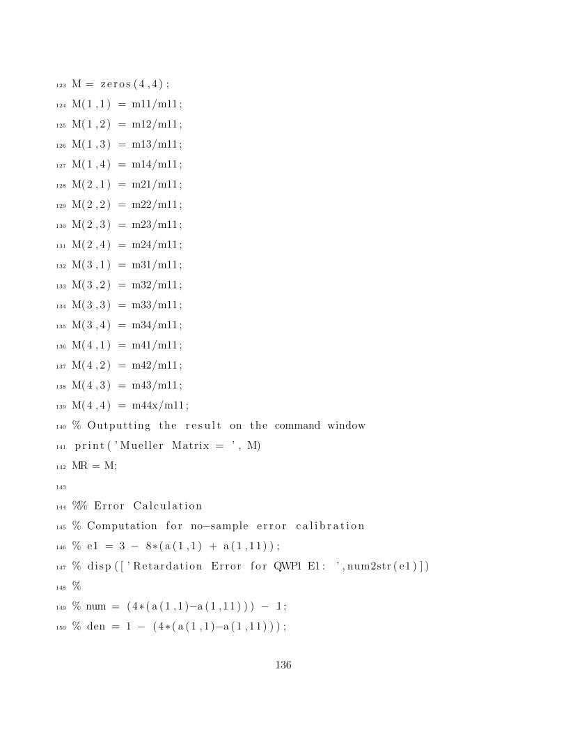
123 M = zero s (4 , 4 ) ;
124 M(1 ,1 ) = m11/m11 ;
125 M(1 ,2 ) = m12/m11 ;
126 M(1 ,3 ) = m13/m11 ;
127 M(1 ,4 ) = m14/m11 ;
128 M(2 ,1 ) = m21/m11 ;
129 M(2 ,2 ) = m22/m11 ;
130 M(2 ,3 ) = m23/m11 ;
131 M(2 ,4 ) = m24/m11 ;
132 M(3 ,1 ) = m31/m11 ;
133 M(3 ,2 ) = m32/m11 ;
134 M(3 ,3 ) = m33/m11 ;
135 M(3 ,4 ) = m34/m11 ;
136 M(4 ,1 ) = m41/m11 ;
137 M(4 ,2 ) = m42/m11 ;
138 M(4 ,3 ) = m43/m11 ;
139 M(4 ,4 ) = m44x/m11 ;
140 % Outputting the r e s u l t on the command window
141 pr in t ( ’ Muel ler Matrix = ’ , M)
142 MR = M;
143
144 %% Error Ca l cu l a t i on
145 % Computation f o r no−sample e r r o r c a l i b r a t i o n
146 % e1 = 3 − 8∗( a (1 , 1 ) + a (1 ,11 ) ) ;
147 % disp ( [ ’ Retardat ion Error f o r QWP1 E1 : ’ , num2str ( e1 ) ] )
148 %
149 % num = (4∗ ( a (1 , 1 )−a (1 ,11 ) ) ) − 1 ;
150 % den = 1 − (4∗ ( a (1 , 1 )−a (1 ,11 ) ) ) ;
136
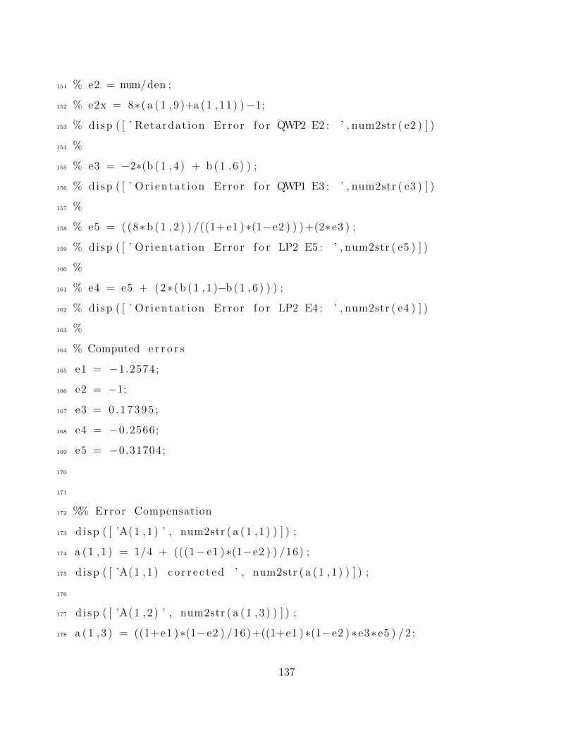
151 % e2 = num/den ;
152 % e2x = 8∗( a (1 , 9 )+a (1 ,11 ) )−1;
153 % disp ( [ ’ Retardat ion Error f o r QWP2 E2 : ’ , num2str ( e2 ) ] )
154 %
155 % e3 = −2∗(b (1 , 4 ) + b (1 , 6 ) ) ;
156 % disp ( [ ’ Or i enta t i on Error f o r QWP1 E3 : ’ , num2str ( e3 ) ] )
157 %
158 % e5 = ((8∗b (1 , 2 ) ) /((1+ e1 )∗(1−e2 ) ) ) +(2∗e3 ) ;
159 % disp ( [ ’ Or i enta t i on Error f o r LP2 E5 : ’ , num2str ( e5 ) ] )
160 %
161 % e4 = e5 + (2∗ ( b (1 , 1 )−b (1 , 6 ) ) ) ;
162 % disp ( [ ’ Or i enta t i on Error f o r LP2 E4 : ’ , num2str ( e4 ) ] )
163 %
164 % Computed e r r o r s
165 e1 = −1.2574;
166 e2 = −1;
167 e3 = 0 . 17395 ;
168 e4 = −0.2566;
169 e5 = −0.31704;
170
171
172 %% Error Compensation
173 di sp ( [ ’A(1 , 1 ) ’ , num2str ( a (1 , 1 ) ) ] ) ;
174 a (1 , 1 ) = 1/4 + (((1− e1 )∗(1−e2 ) ) /16) ;
175 di sp ( [ ’A(1 , 1 ) c o r r e c t e d ’ , num2str ( a (1 , 1 ) ) ] ) ;
176
177 di sp ( [ ’A(1 , 2 ) ’ , num2str ( a (1 , 3 ) ) ] ) ;
178 a (1 , 3 ) = ((1+ e1 )∗(1−e2 ) /16)+((1+e1 )∗(1−e2 ) ∗ e3∗ e5 ) /2 ;
137
179 di sp ( [ ’A(1 , 2 ) c o r r e c t e d ’ , num2str ( a (1 , 3 ) ) ] ) ;
180
181 di sp ( [ ’A(1 , 8 ) ’ , num2str ( a (1 , 9 ) ) ] ) ;
182 a (1 , 9 ) = (1+e1 ) ∗(1+e2 ) /16 ;
183 di sp ( [ ’A(1 , 8 ) c o r r e c t e d ’ , num2str ( a (1 , 9 ) ) ] ) ;
184
185
186 di sp ( [ ’A(1 ,10 ) ’ , num2str ( a (1 , 11 ) ) ] ) ;
187 a (1 ,11 ) = (1−e1 ) ∗(1+e2 ) /16 ;
188 di sp ( [ ’A(1 ,10 ) c o r r e c t e d ’ , num2str ( a (1 , 11 ) ) ] ) ;
189
190 di sp ( [ ’B(1 , 4 ) ’ , num2str (b (1 , 4 ) ) ] ) ;
191 b (1 , 4 ) = ( e4−e3−e5 ) /4 ;
192 di sp ( [ ’B(1 , 4 ) c o r r e c t e d ’ , num2str (b (1 , 4 ) ) ] ) ;
193
194 di sp ( [ ’B(1 , 6 ) ’ , num2str (b (1 , 6 ) ) ] ) ;
195 b (1 , 6 ) = ( e5−e3−e4 ) /4 ;
196 di sp ( [ ’B(1 , 6 ) c o r r e c t e d ’ , num2str (b (1 , 6 ) ) ] ) ;
197
198 di sp ( [ ’B(1 , 8 ) ’ , num2str (b (1 , 8 ) ) ] ) ;
199 b (1 , 8 ) = ((1+ e1 ) ∗(1+e2 ) ∗(2∗ e4 − 2∗e3−e5 ) ) /8 ;
200 di sp ( [ ’B(1 , 8 ) c o r r e c t e d ’ , num2str (b (1 , 8 ) ) ] ) ;
201
202 di sp ( [ ’B(1 , 2 ) ’ , num2str (b (1 , 2 ) ) ] ) ;
203 b (1 , 2 ) = −(((1+e1 )∗(1−e2 ) ∗ e3 ) /4) + (((1+ e1 )∗(1−e2 ) ∗ e5 ) /8) ;
204 di sp ( [ ’B(1 , 2 ) c o r r e c t e d ’ , num2str (b (1 , 2 ) ) ] ) ;
205
206 di sp ( [ ’B(1 ,10 ) ’ , num2str (b (1 ,10 ) ) ] ) ;
138
207 b (1 ,10 ) = −((1−e1 ) ∗(1+e2 ) ∗ ( (2∗ e4 )−e5 ) ) /8 ;
208 di sp ( [ ’B(1 ,10 ) c o r r e c t e d ’ , num2str (b (1 ,10 ) ) ] ) ;
209
210 %% Obtaining Error Compensated Muel ler components from
211 % the new Four i e r C o e f f i c i e n t s
212 m11 = a (1 , 1 )−a (1 , 3 )+a (1 , 9 )−a (1 ,11 )+a (1 ,13 ) ;
213 m12 = 2∗a (1 , 3 ) − 2∗a (1 , 9 ) − 2∗a (1 ,13 ) ;
214 m13 = 2∗b (1 , 2 ) +2∗b (1 , 8 )−2∗b (1 ,12 ) ;
215 m14 = b (1 , 1 )−2∗b (1 ,11 ) ;
216 m14x = b (1 , 1 ) +2∗b (1 , 9 ) ;
217 m14x2 = b (1 , 1 )+b (1 , 9 )−b (1 ,11 ) ;
218 m21 = −2∗a (1 , 9 ) +2∗a (1 ,11 )−2∗a (1 ,13 ) ;
219 m22 = 4∗a (1 , 9 ) +4∗a (1 ,13 ) ;
220 m23 = −4∗b (1 , 8 ) +4∗b (1 ,12 ) ;
221 m24 = 2∗(−1∗b (1 , 9 )+b (1 ,11 ) ) ;
222 m24x = −4∗b (1 , 9 ) ;
223 m24x2 = 4∗b (1 ,11 ) ;
224 m31 = −2∗b (1 , 8 ) +2∗b (1 ,10 )−2∗b (1 ,12 ) ;
225 m32 = 4∗b (1 , 8 ) +4∗b (1 ,12 ) ;
226 m33 = 4∗a (1 , 9 )−4∗a (1 ,13 ) ;
227 m34 = 4∗a (1 ,10 ) ;
228 m34x = −4∗a (1 ,12 ) ;
229 m34x2 = 2∗( a (1 , 10 )−a (1 ,12 ) ) ;
230 m41 = 2∗b (1 , 3 )−b (1 , 5 ) ;
231 m41x = b (1 , 3 )−b (1 , 5 )+b (1 , 7 ) ;
232 m41x2 = −1∗b (1 , 5 ) +2∗b (1 , 7 ) ;
233 m42 = −4∗b (1 , 7 ) ;
234 m42x = −4∗b (1 , 3 ) ;
139

235 m42x2 = −2∗(b (1 , 3 )+b (1 , 7 ) ) ;
236 m43 = −4∗a (1 , 4 ) ;
237 m43x = 4∗a (1 , 8 ) ;
238 m43x2 = 2∗(−1∗a (1 , 4 )+ a (1 , 8 ) ) ;
239 m44 = −2∗a (1 , 5 ) ;
240 m44x = 2∗a (1 , 7 ) ;
241 m44x2 = a (1 , 7 )−a (1 , 5 ) ;
242 %% Normal izat ion
243 Mu = ze ro s (4 , 4 ) ;
244 Mu(1 ,1 ) = m11 ;
245 Mu(1 ,2 ) = m12 ;
246 Mu(1 ,3 ) = m13 ;
247 Mu(1 ,4 ) = m14 ;
248 Mu(2 ,1 ) = m21 ;
249 Mu(2 ,2 ) = m22 ;
250 Mu(2 ,3 ) = m23 ;
251 Mu(2 ,4 ) = m24 ;
252 Mu(3 ,1 ) = m31 ;
253 Mu(3 ,2 ) = m32 ;
254 Mu(3 ,3 ) = m33 ;
255 Mu(3 ,4 ) = m34 ;
256 Mu(4 ,1 ) = m41 ;
257 Mu(4 ,2 ) = m42 ;
258 Mu(4 ,3 ) = m43 ;
259 Mu(4 ,4 ) = m44 ;
260 pr in t ( ’Non−Normalized Error Compensated Muel ler Matrix = ’ ,Mu)
261 %% I n s e r t i n g the mue l l e r components in to an M matrix
262 M = zero s (4 , 4 ) ;
140

263 M(1 ,1 ) = m11/m11 ;
264 M(1 ,2 ) = m12/m11 ;
265 M(1 ,3 ) = m13/m11 ;
266 M(1 ,4 ) = m14/m11 ;
267 M(2 ,1 ) = m21/m11 ;
268 M(2 ,2 ) = m22/m11 ;
269 M(2 ,3 ) = m23/m11 ;
270 M(2 ,4 ) = m24/m11 ;
271 M(3 ,1 ) = m31/m11 ;
272 M(3 ,2 ) = m32/m11 ;
273 M(3 ,3 ) = m33/m11 ;
274 M(3 ,4 ) = m34/m11 ;
275 M(4 ,1 ) = m41/m11 ;
276 M(4 ,2 ) = m42/m11 ;
277 M(4 ,3 ) = m43/m11 ;
278 M(4 ,4 ) = m44/m11 ;
279 % Outputting the r e s u l t on the command window
280 pr in t ( ’ Normalized Error Compensated Muel ler Matrix = ’ , M) ;
This function performs the Mueller matrix correction for the known CPR vs phase
angle datasets of analog samples. The program uses Stokes vector of the entire dataset
over 0-5 degree phase angles to compute the corrected Stokes vector from which CPR
values are calculated. Mueller matrix parameters are used from the previous Mueller
matrix computation program while Stokes vectors are acquired from the Stokes vector
computation program. [39]
1 %% Muel ler Matrix Correc t ion Program
2 % by Mrunal Amin
3
4 % Function takes Muel ler Matrix o f the o p t i c a l element to be
141
c o r r e c t e d
5 % CPR and t h e i r r e s p e c t i v e phase ang le va lue s
6 f unc t i on [CPRN] = MMcorrection (MM, angle , CPR)
7
8 S4 = ze ro s ( l ength ( ang le ) , 1 ) ;
9
10 f o r k = 1 : l ength ( ang le )
11 S4 (k , 1 ) = (1−CPR(k , 1 ) ) /(1+CPR(k , 1 ) ) ;
12 end
13
14 % Mult ip ly ing the i n v e r s e o f Muel ler matrix with output Stokes
vec to r
15 % r e s u l t s in input Stokes vec to r
16 RS = ze ro s ( l ength ( ang le ) , 4 ) ;
17 f o r j = 1 : l ength ( ang le )
18 RS( j , : ) = inv (MM) ∗ [ 1 ; 0 .3∗ S4 ( j , 1 ) ; 0 .3∗ S4 ( j , 1 ) ; S4 ( j , 1 ) ] ;
19 end
20
21 RX = ze ro s ( l ength ( ang le ) , 4 ) ;
22 f o r b = 1 : l ength ( ang le )
23 RX(b , : ) = RS(b , : ) /RS(b , 1 ) ;
24 end
25
26 % New c o r r e c t e d CPR va lues
27 CPRN = ze ro s ( l ength ( ang le ) , 1 ) ;
28 f o r l = 1 : l ength ( ang le )
29 CPRN( l , 1 ) = (RX( l , 1 ) + RX( l , 4 ) ) /(RX( l , 1 )− RX( l , 4 ) ) ;
30 end
142
31 end
1 % F i t t i n g a curve to the miss ing data po in t s by method o f l e a s t
squares
2 % Least Squares
3 f unc t i on [ LS ] = LeastSquaresF i t ( ang , dataX , xq )
4
5 % Taking 5 meas va lue s be f o r e and a f t e r to get the Least Squares
Regres s ion
6 % Deta i l ed exp lanat ion goes here
7 Y = dataX ’ ;
8 X = ang ’ ;
9 H= [ ] ;
10 % N s t a t e s the order o f the exp r e s s i on eva luated
11 N = 5 ;
12 f o r i = 0 :N
13 H = [H,X. ˆ i ] ;
14 end
15 % H = [ ones ( l ength (Y) ,1 ) ,X,X. ˆ 2 , X. ˆ 3 ) ;
16 Astar = inv (H’∗H) ∗H’∗Y;
17
18 Yt i lde = H∗Astar ;
19
20 % R p r i n t s the r e s i d u a l
21 R = sum ( (Y−Yt i lde ) . ˆ 2 ) ;
22 LS = int e rp1 (X, Yti lde , xq , ’ poly5 ’ , ’ extrap ’ ) ;
23 end
143
Related Documents