AMERICAN STEP-UP AND STEP-DOWN CREDIT DEFAULT SWAPS UNDER L ´ EVY MODELS TIM S.T. LEUNG † AND KAZUTOSHI YAMAZAKI ‡ ABSTRACT. This paper studies the valuation of a class of credit default swaps (CDSs) with the embedded option to switch to a different premium and notional principal anytime prior to a credit event. These are early exercisable contracts that give the protection buyer or seller the right to step-up, step-down, or cancel the CDS position. The pricing problem is formulated under a structural credit risk model based on L´ evy processes. This leads to the analytic and numerical studies of several optimal stopping problems subject to early termination due to default. In a general spectrally negative L´ evy model, we rigorously derive the optimal exercise strategy. This allows for instant computation of the credit spread under various specifica- tions. Numerical examples are provided to examine the impacts of default risk and contractual features on the credit spread and exercise strategy. Keywords: optimal stopping; credit default swaps; step-up and step-down options; L´ evy processes; scale func- tions JEL Classification: G13, G33, D81, C61 Mathematics Subject Classification (2000): 60G51 91B25 91B70 Date: December 25, 2010. † Department of Applied Mathematics & Statistics, Johns Hopkins University, Baltimore MD 21218, USA. Email: [email protected]. ‡ Center for the Study of Finance and Insurance, Osaka University, 1-3 Machikaneyama-cho, Toyonaka City, Osaka 560- 8531, Japan. Email: [email protected] . The authors would like to thank Prof. Goran Peskir for reading the first draft and for his helpful remarks and suggestions. This work is partially supported by NSF grant DMS-0908295 and by Grant-in-Aid for Young Scientists (B) No. 22710143, the Ministry of Education, Culture, Sports, Science and Technology. 1

Welcome message from author
This document is posted to help you gain knowledge. Please leave a comment to let me know what you think about it! Share it to your friends and learn new things together.
Transcript

AMERICAN STEP-UP AND STEP-DOWN CREDIT DEFAULT SWAPS UNDER LEVYMODELS
TIM S.T. LEUNG† AND KAZUTOSHI YAMAZAKI‡
ABSTRACT. This paper studies the valuation of a class of credit default swaps (CDSs) with the embedded
option to switch to a different premium and notional principal anytime prior to a credit event. These are
early exercisable contracts that give the protection buyer or seller the right to step-up, step-down, or cancel
the CDS position. The pricing problem is formulated under a structural credit risk model based on Levy
processes. This leads to the analytic and numerical studies of several optimal stopping problems subject
to early termination due to default. In a general spectrally negative Levy model, we rigorously derive the
optimal exercise strategy. This allows for instant computation of the credit spread under various specifica-
tions. Numerical examples are provided to examine the impacts of default risk and contractual features on
the credit spread and exercise strategy.
Keywords: optimal stopping; credit default swaps; step-up and step-down options; Levy processes; scale func-
tions
JEL Classification: G13, G33, D81, C61
Mathematics Subject Classification (2000): 60G51 91B25 91B70
Date: December 25, 2010.† Department of Applied Mathematics & Statistics, Johns Hopkins University, Baltimore MD 21218, USA. Email:
‡Center for the Study of Finance and Insurance, Osaka University, 1-3 Machikaneyama-cho, Toyonaka City, Osaka 560-
8531, Japan. Email: [email protected] .
The authors would like to thank Prof. Goran Peskir for reading the first draft and for his helpful remarks and suggestions.
This work is partially supported by NSF grant DMS-0908295 and by Grant-in-Aid for Young Scientists (B) No. 22710143,
the Ministry of Education, Culture, Sports, Science and Technology.1

2 T. LEUNG AND K. YAMAZAKI
CONTENTS
1. Introduction 3
2. Problem Overview 5
2.1. Credit Default Swaps and Swaptions 5
2.2. American Callable Step-Up and Step-Down CDS 7
2.3. The American Putable Step-Up/Down CDS 9
2.4. Symmetry Between Callable and Putable CDS 10
2.5. Solution Methods via Continuous and Smooth Fit 11
3. Solution Methods under the Spectrally Negative Levy Model 13
3.1. The Spectrally Negative Levy Process and Scale Function 13
3.2. Callable Step-Down CDS 15
3.3. Putable Step-Down CDS 20
4. Numerical Examples 23
4.1. Spectrally negative Levy processes with hyperexponential jumps 23
4.2. Hyperexponential Fitting 25
4.3. Numerical Results 25
5. Concluding Remarks 31
Appendix A. Proofs 31
A.1. Proofs for Section 2 31
A.2. Proofs for Subsection 3.2 32
A.3. Proofs for Subsection 3.3 36
References 38

AMERICAN STEP-UP AND STEP-DOWN CDS 3
1. INTRODUCTION
Credit default swaps (CDSs) are among the most liquid and widely used instruments for managing and trans-
ferring credit risks. Despite the recent market turbulence, their market size still exceeds US$30 trillions1. In a
standard single-name CDS, the protection buyer pays a pre-specified periodic premium (the CDS spread) to the
protection seller to cover the loss of the face value of an asset if the reference entity defaults before expiration.
The contract stipulates that both the buyer and seller have to commit to their respective positions until the default
time or expiration date. To modify the initial CDS exposure in the future, one common way is to acquire appropri-
ate positions later from the market, but it is subject to credit spread fluctuations and market illiquidity, especially
during adverse market conditions.
To provide additional flexibility to investors, credit default swaptions and other derivatives on CDSs have
emerged. For instance, the payer (receiver) default swaption is a European option that gives the holder the right to
buy (sell) protection at a pre-specified strike spread at expiry, given that default has not occurred. Otherwise, the
swaption is knocked out. See, for example, [22]. By appropriately combining a default swaption with a vanilla
CDS position, one can create a callable or putable default swap. A callable (putable) CDS allows the protection
buyer (seller) to terminate the contract at some fixed future date. Hence, as described here, the callable/putable
CDSs are in fact cancellable CDSs. Typically, the callable feature is paid for through incremental premium on top
of the standard CDS spread, so selling a callable CDS can enhance the yield from the seller’s perspective.
In this paper, we consider a class of CDSs embedded with an option for the investor (protection buyer or seller) to
adjust the premium and notional amount once for a pre-specified fee prior to default. Specifically, these contracts
equip the standard default swaps with the early exercisable rights such as (i) the step-up option that allows the
investor to increase the protection and premium at exercise, and (ii) the step-down option to reduce the protection
and premium. By definition, these contracts are indeed generalized versions of the callable and putable CDSs
mentioned above, and thus are more flexible credit risk management tools. Henceforth, we shall use the more
general meaning of the terminology callable and putable CDSs, rather than limiting them to cancellable CDSs.
The main contribution of our paper is to determine the credit spread for these CDSs under a Levy model,
and analyze the optimal strategy for the buyer or seller to exercise the step-up/down option. Specifically, we
model the default time as the first passage time of a Levy process representing some underlying asset value. We
decompose the CDS with step-up/down option into a combination of an American-style credit default swaption
and a vanilla CDS. From the investor’s perspective, this gives rise to an optimal stopping problem subject to
possible sudden early termination from default risk. Our formulation is based on a general Levy process, and then
1According to the ISDA Market Survey, the total CDS outstanding volume in 2009 is US$30,428 billions.
4 T. LEUNG AND K. YAMAZAKI
we solve analytically for a general spectrally negative Levy process. By employing the scale function and other
properties of Levy processes, we derive analytic characterization for the optimal exercising strategy. This in turn
allows for a highly efficient computation of the credit spread for these CDS contracts. We provide a series of
numerical examples to illustrate the credit spread behavior and optimal exercising strategy under various contract
specifications and scenarios.
We adopt a Levy-based structural credit risk model that extends the original approach introduced by Black and
Cox [10] where the asset value follows a geometric Brownian motion. Other structural default models based on
Levy and other jump processes can also be found in [12, 20, 42]. To our best knowledge, the valuation of American
step-up and step-down CDSs has not been studied elsewhere. For Levy-based pricing models for other credit
derivatives, such as European credit default swaptions and collateralized debt obligations (CDOs), we highlight
[3, 15, 25], among others.
Levy processes have been widely applied in derivatives pricing. Some well-known examples of Levy pricing
models include the variance gamma (VG) model [33], the normal inverse Gaussian (NIG) model [7], the CGMY
model [14] as well as a number of jump diffusion models (see [27, 34]). In this paper, instead of focusing on a
particular type of Levy process, we consider a general class of Levy processes with only negative jumps. This is
called the spectrally negative Levy process and has been drawing much attention recently, as a generalization of
the classical Cramer-Lundberg and other compound-Poisson type processes. A number of fluctuation identities
can be expressed in terms of the scale function and are used in a number of applications. We refer the reader to
[1, 5] for derivative pricing, [30] for optimal capital structure, [8, 9] for stochastic games, [6, 29, 32] for optimal
dividend problem, and [16] for optimal timing of capital reinforcement. For a comprehensive account, see [28].
A major component of our pricing problem involves a non-standard American option subject to default risk (see
Proposition 2.1). This is related to some existing work on perpetual early exercisable options under various Levy
models, for example [2, 5, 11, 35]. The infinite horizon nature of these problems provides significant convenience
for analysis and sometimes permits an explicit solution. For finite maturity American options, the solution can be
obtained by solving the underlying partial integral differential equation (PIDE) or by other approximation methods;
see for example [4, 21, 23]. In our model, the solution is analytic for a general spectrally negative Levy process.
For numerical examples, we select the phase-type (and hyperexponential) fitting approach by Egami and Yamazaki
[17] to illustrate the cases when the process is a mixture of diffusion and a compound Poisson process with Pareto-
distributed jumps.
The rest of the paper is organized as follows. In Section 2, we formulate the default swap valuation problems
under a general Levy model. In Section 3, we focus on the spectrally negative Levy model and provide a complete
solution and detailed analysis. Section 4 provides the numerical results along with a discussion on numerical
AMERICAN STEP-UP AND STEP-DOWN CDS 5
approximation of scale functions. Section 5 concludes the paper and presents some extensions of our model. Most
proofs are deferred to the Appendix.
2. PROBLEM OVERVIEW
Let (Ω,F ,P) be a complete probability space, where P is the risk-neutral measure used for pricing. We assume
there exists a Levy process X = Xt; t ≥ 0, and denote by F = (Ft)t≥0 the filtration generated by X . The value
of the reference entity (a company stock or other assets) is assumed to evolve according to an exponential Levy
process St = eXt , t ≥ 0. Following the Black-Cox [10] structural approach, the default event is triggered by S
crossing a lower level D, so the default time is given by the first passage time: θD := inf t ≥ 0 : Xt ≤ logD .
Without loss of generality, we can take logD = 0 by shifting the initial value x. Henceforth, we shall work with
the default time:
θ := inf t ≥ 0 : Xt ≤ 0 ,
where we assume inf ∅ =∞. Throughout this paper, we denote by Px the probability law and Ex the expectation
under which X0 = x.
2.1. Credit Default Swaps and Swaptions. In preparation for CDS with step-up/down options, let us start with
the basic concepts of credit default swaps and swaptions. Under a T -year credit default swap (CDS) on a unit
face value, the protection buyer pays a constant premium payment $p continuously over time until default time
θ or maturity T , whichever comes first. If default occurs before T , the buyer will receive the default payment
α := 1−R at time θ, whereR is the assumed constant recovery rate (typically 40%). From the buyer’s perspective,
the expected discounted payoff is given by
C(x; p, α, T ) := Ex[−∫ θ∧T
0e−rtp dt+ αe−rθ1θ≤T
],
where r > 0 is the positive constant risk-free interest rate. The quantity C(x; p, α, T ) can be viewed as the market
price for the buyer to enter (or long) a CDS with an agreed premium p, default payment α and maturity T . On the
opposite side of the trade, the protection seller’s expected cash flow is −C(x; p, α, T ) = C(x;−p,−α, T ) ∈ R.
In standard practice, the CDS spread p is determined at inception such that C(x; p, α, T ) = 0, yielding zero
expected cash flows for both parties. Direct calculations show that the credit spread can be expressed as
p(x;α, T ) =α r ζT (x)
1− ζT (x)− e−rTPxθ > T, where ζT (x) := Ex
[e−rθ1θ≤T
].(2.1)
For most Levy models, due to the lack of explicit formulas, the computation of the CDS spread is based on
simulation or other approximation methods (see, for example, [12]). Alternatively, one can consider the perpetual

6 T. LEUNG AND K. YAMAZAKI
case as an approximation. This is a popular approach adopted for equity derivatives, especially American options,
for which the finite-maturity contracts do not admit closed-form solutions while the perpetual versions often do.
To illustrate, we set T = +∞ and express the buyer’s CDS price as
C(x; p, α) := Ex[−∫ θ
0e−rtp dt+ α e−rθ
](2.2)
=(pr
+ α)ζ(x)− p
r,
where
ζ(x) := Ex[e−rθ
].(2.3)
The seller’s CDS price is −C(x; p, α) = C(x;−p,−α) ∈ R. Solving C(x; p, α) = 0 yields the credit spread:
p(x;α) =α r ζ(x)
1− ζ(x).(2.4)
Therefore, the credit spread calculation reduces to computing the Laplace transform ζ(x), which admits an explicit
analytic formula under some well-known Levy models (see (3.4) below for the spectrally negative case). It is clear
from (2.4) that the CDS spread scales linearly in α: p(x;α) = αp(x; 1).
Next, we introduce a perpetual American payer and receiver default swaptions, which give the holder the right
to, respectively, buy and sell protection on a perpetual CDS with default payment a at a pre-specified spread κ for
the strike price K upon exercise. If default occurs prior to exercise, then the swaption is knocked out and becomes
worthless. The payer and receiver swaption holder is required to pay an upfront fee, which is given by respectively
v(x;κ, a,K) := supτ∈S
Ex[e−rτ (C(Xτ ;κ, a)−K)+ 1τ<θ
], and(2.5)
u(x;κ, a,K) := supτ∈S
Ex[e−rτ (−C(Xτ ;κ, a)−K)+ 1τ<θ
],(2.6)
where S := τ ∈ F : τ ≤ θ a.s. is the set of all stopping times smaller than or equal to the default time. The
two price functions are related by
v(x;κ, a,K) = u(x;−κ,−a,K).(2.7)
In summary, v(x;κ, a,K) is the payer default swaption price when κ, a ≥ 0, and it is the receiver default swaption
price when κ, a ≤ 0.

AMERICAN STEP-UP AND STEP-DOWN CDS 7
2.2. American Callable Step-Up and Step-Down CDS. Next, we consider a CDS contract with an embedded
option that permits the protection buyer to change the face value and premium once for a fee. Beginning from
initiation, the buyer pays a premium p for a protection of a unit face value. At any time prior to default, the buyer
can select a time τ to switch to a new contract with a new premium p and face value q for a fee γ. The default
payment then changes from α to α = qα after the exercise time τ . Here, p, α, γ, α, and p are constant non-negative
parameters pre-specified at time zero. The buyer’s maximal expected cash flow is given by
V (x; p, p, α, α, γ)(2.8)
:= supτ∈S
Ex[−∫ τ
0e−rtp dt+ 1τ<∞
(−∫ θ
τe−rtp dt− e−rτγ1τ<θ + e−rθ(α1τ<θ + α1τ=θ)
)].
This formulation covers default swaps with the following provisions:
(1) Step-up Option: if p > p and α > α, then the buyer is allowed to increase the coverage once from α to α
by paying the fee γ and a higher premium p thereafter.
(2) Step-down Option: when p < p and α < α, then the buyer can reduce the coverage once from α to α by
paying the fee γ and a reduced premium p thereafter.
(3) Cancellation Right: as a special case of the step-down option with p = α = 0, the resulting contract
allows the buyer to terminate the CDS at time τ .
In addition, the perpetual vanilla CDS corresponds to the case with γ = 0, p = p and α = α, and the CDS spread is
given by (2.4). We ignore the contract specifications with (p− p)(α−α) ≤ 0 since they would mean paying more
(less) premium in exchange for a reduced (increased) protection after exercise. In summary, we study the valuation
of the (perpetual) American callable step-up/down CDS. For any fixed parameters (p, p, α, α, γ), the value V (x) is
referred to as the buyer’s price, so the seller’s price is−V (x). The credit spread p∗ is determined from the equation
V (x; p∗, p, α, α, γ) = 0 so that no cash transaction occurs at inception.
In preparation for our solution procedure, we first provide a useful representation of the buyer’s value V . Define
α := α− α, and p := p− p.
Here, α > 0 and p > 0 hold for a step-down CDS and α < 0 and p < 0 for a step-up CDS.
Proposition 2.1. The perpetual American callable step-up/down CDS can be decomposed into a vanilla CDS plus
a perpetual American payer/receiver swaption. Precisely, we have
V (x; p, p, α, α, γ) = C(x; p, α) + v(x;−p,−α, γ),(2.9)
where C(·) and v(·) are given in (2.2) and (2.5) respectively.

8 T. LEUNG AND K. YAMAZAKI
Proof. First, by a rearrangement of integrals, the expression inside the expectation in (2.8) becomes
1τ<∞
(∫ θ
τe−rtp dt−
∫ θ
0e−rtp dt− e−rτγ1τ<θ − e−rθα1τ<θ + e−rθα
)+ 1τ=∞
(−∫ ∞
0e−rtp dt
)= 1τ<∞
(∫ θ
τe−rtp dt− e−rτγ1τ<θ − e−rθα1τ<θ
)−∫ θ
0e−rtp dt+ e−rθα
since τ =∞ implies θ =∞ by the definition of S. Because the last two terms do not depend on τ , we can rewrite
the buyer’s value function as
V (x) = supτ∈S
Ex[1τ<∞
(∫ θ
τe−rtp dt− e−rτγ1τ<θ − e−rθα1τ<θ
)]︸ ︷︷ ︸
=:f(x)
−Ex[∫ θ
0e−rtp dt
]+ αEx
[e−rθ
].
Here, the last two terms in fact constitute C(x; p, α). Next, using the fact τ < θ, τ <∞ = Xτ > 0, τ <∞
for every τ ∈ S and the strong Markov property of X at time τ , we rewrite the first term as
f(x) = supτ∈S
Ex[e−rτh(Xτ )1τ<∞
],(2.10)
with
h(x) := 1x>0
(Ex[∫ θ
0e−rtpdt − e−rθα
]− γ)
= 1x>0(C(x;−p,−α)− γ
).(2.11)
Since θ ∈ S and h(Xθ) = 0 a.s. on θ < ∞, it follows from (2.10) that f(x) ≥ 0. Therefore, it is never
optimal to exercise at any τ if h(Xτ ) < 0. Consequently, we can replace h(x) with (h(x))+ in (2.10). As a result,
with −p,−α > (<) 0, the function f(x) is indeed the price of a perpetual American payer (receiver) default
swaption written on the buyer’s (seller’s) CDS price with strike γ ≥ 0. This implies that f(x) = v(x;−p,−α, γ)
∀x ∈ R, and therefore (2.9) follows.
The decomposition (2.9) in Proposition 2.1 yields a static replication of the American callable step-up/down
CDS. To this end, one may also verify the result by a no-arbitrage argument. We summarize the buyer’s and
seller’s positions in the American callable step-up/down CDS in Table 1.
Proposition 2.1 also provides some insight on the protection buyer’s exercise timing. To illustrate, let us consider
an example where the premium and protection are doubled after exercise, i.e. p = 2p and α = 2α. For any
candidate exercise time τ , the observable market prevailing vanilla CDS spread is given by p(Xτ ;α) in (2.4), and
C(Xτ ; p(Xτ ;α), α) = 0 by definition. Hence, if p(Xτ ;α) ≤ −p = p at τ , then h(Xτ ) ≤ −γ ≤ 0, and the
buyer will not exercise. This is intuitive because the buyer is better off giving up the step-up option and double his
protection by entering a separate CDS at the lower market spread p(Xτ ;α) at time τ .

AMERICAN STEP-UP AND STEP-DOWN CDS 9
Protection Buyer’s Position Protection Seller’s Position
American Callable long a vanilla CDS & short a vanilla CDS &
Step-Up CDS long an American payer default swaption short an American payer default swaption
American Callable long a vanilla CDS & short a vanilla CDS &
Step-Down CDS long an American receiver default swaption short an American receiver default swaption
TABLE 1. Four positions of American callable step-up/down CDS and their decompositions.
The seller’s position is the opposite of the buyer’s.
2.3. The American Putable Step-Up/Down CDS. Applying the ideas from the previous subsection, we formu-
late the pricing problem for the perpetual American putable step-up/down CDS. These CDSs allow the protection
seller (and not the buyer) to change the protection premium and default payment for a fee anytime prior to default.
Let p and α be the initial premium and default payment. The seller may select a time τ to switch to a new premium
p and default payment α for a switching fee γ ≥ 0. The seller’s maximal expected cash flow is
U(x; p, p, α, α, γ)(2.12)
:= supτ∈S
Ex[∫ τ
0e−rtp dt+ 1τ<∞
(∫ θ
τe−rtpdt− e−rτγ1τ<θ − e−rθ(α1τ<θ + α1τ=θ)
)]= sup
τ∈SEx[1τ<∞
(−∫ θ
τe−rtp dt− e−rτγ1τ<θ + e−rθα1τ<θ
)]+ Ex
[∫ θ
0e−rtp dt
]− αEx
[e−rθ
].
In particular, we will study the American putable CDS with a step-up option (i.e. p < p and α < α) or step-
down option (i.e. p > p and α > α). Again, the credit spread p∗ is chosen so that the seller’s value function is
zero, i.e. U(x; p∗, p, α, α, γ) = 0.
Following the procedure in the proof of Proposition 2.1 or by a no-arbitrage argument, we can simplify the
seller’s value U as follows:
Proposition 2.2. The perpetual American putable step-up/down CDS can be decomposed into a short vanilla CDS
and a long perpetual American receiver/payer default swaption. Precisely, we have
U(x; p, p, α, α, γ) = −C(x; p, α) + u(x;−p,−α, γ),(2.13)
where C(·) and u(·) are given in (2.2) and (2.6), respectively.

10 T. LEUNG AND K. YAMAZAKI
Protection Buyer’s Position Protection Seller’s Position
American Putable long a vanilla CDS & short a vanilla CDS &
Step-Up CDS short an American receiver default swaption long an American receiver default swaption
American Putable long a vanilla CDS & short a vanilla CDS &
Step-Down CDS short an American payer default swaption long an American payer default swaption
TABLE 2. Four positions of American putable step-up/down CDS and their decompositions. The
seller’s position is the opposite of the buyer’s.
We summarize the buyer’s and seller’s positions in the American putable step-up/down CDS in Table 2. To gain
intuition on the seller’s exercise decision, let us look at the step-down case where p = 0.5p and α = 0.5α. Recall
that C(x; p, α) is decreasing in p and C(Xτ , p(Xτ ;α), α) = 0 for any stopping time τ . If the market prevailing
CDS spread p(Xτ ;α) ≤ p at some τ , then the seller’s default swaption payoff is −C(Xτ ; p, α) − γ ≤ −γ ≤ 0.
The seller will not exercise at τ since the protection of 0.5α can be purchased from a separate CDS at the lower
prevailing spread 0.5p(Xτ ;α) ≤ 0.5p.
2.4. Symmetry Between Callable and Putable CDS. By Propositions 2.1 and 2.2, along with (2.7), we observe
the following “put-call parity” and symmetry identities:
V (x; p, p, α, α, γ)− U(x; p, 2p− p, α, 2α− α, γ) = 2C(x; p, α),
V (x; p, p, α, α, γ) + U(x; p, 2p− p, α, 2α− α, γ) = 2 v(x; p− p, α− α, γ).
The first equality means a long position in an American callable step-up (step-down) CDS and a short position
in an American putable step-down (step-up) CDS result in a double long position in a vanilla CDS. From the
second equality, a long position in both an American callable step-up (step-down) CDS and an American putable
step-down (step-up) CDS yields a double long position in an American payer (receiver) default swaption.
Furthermore, according to (2.9) and (2.13), the optimal exercise times for V (x) and U(x) are determined from
v(x) and u(x) which depend on the triplet (p, α, γ) but not directly on p and α. Consequently, by (2.7), the same
optimal exercising strategy applies for both
(1) the protection buyer of an American callable CDS with a step-up (step-down) option with (−p,−α, γ),
and
(2) the protection seller of an American putable CDS with a step-down (step-up) option with (p, α, γ).
This observation means that it suffices to solve for two cases instead of four. Specifically, we shall solve for (i) the
buyer’s callable step-down case in (2.9) and (ii) the seller’s putable step-down case in (2.13), both with p > 0 and

AMERICAN STEP-UP AND STEP-DOWN CDS 11
α > 0. In view of (2.10) and the proof of Proposition 2.1, this amounts to solving the following optimal stopping
problems:
v(x) := v(x;−p,−α, γ) = supτ∈S
Ex[e−rτh(Xτ )1τ<∞
],(2.14)
u(x) := u(x;−p,−α, γ) = supτ∈S
Ex[e−rτg(Xτ )1τ<∞
],(2.15)
where p, α > 0 and
h(x) :=
((p
r− γ)−(p
r+ α
)ζ(x)
)1x>0,(2.16)
g(x) :=
((− pr− γ)
+
(p
r+ α
)ζ(x)
)1x>0,(2.17)
for x ∈ R. Here, h(x) and g(x) are computed using formula (2.2).
By inspecting (2.14), it follows from (2.16) that h(x) ≤ 0 ∀x ∈ R if γ ≥ p/r. Financially, this means that the
fee γ to be paid exceeds the maximum benefit of stepping down, i.e. perpetual annuity with premium p− p > 0. It
is clear that choosing τ = θ is optimal and the protection buyer will never exercise the step-down option. Hence,
we only need to study the non-trivial case with the condition
0 ≤ γ < p
r.(2.18)
For (2.15), we have g(x) ≤ 0 ∀x ∈ R if g(0+) ≤ 0 because g is decreasing in x on (0,∞). Again, this means
that θ is automatically optimal for the protection seller. Therefore, we shall focus on the case with g(0+) > 0
which also implies
0 ≤ γ < α.(2.19)
The intuition behind this is that the fee should not exceed the reduction in liability.
2.5. Solution Methods via Continuous and Smooth Fit. We conclude this section by describing our solution
procedure for the optimal stopping problems under a general Levy model. In the next section, we shall focus on
the spectrally negative Levy model and derive an analytical solution.
For our first problem (2.14), the protection buyer has an incentive to step-down when default is less likely, or
equivalently when X is sufficiently high. Following this intuition, we denote the threshold strategy
τ+B := inf t ≥ 0 : Xt /∈ (0, B) , B ≥ 0.(2.20)
Clearly, τ+B ∈ S. The corresponding expected payoff is given by
vB(x) := Ex[e−rτ
+B h(Xτ+B
)1τ+B<∞
], x ∈ R.(2.21)

12 T. LEUNG AND K. YAMAZAKI
Note that vB(x) = h(x) = 0 for x ≤ 0. Sometimes it is more intuitive to consider the difference
∆B(x) := vB(x)− h(x), x ∈ R.
One common solution approach for many optimal stopping problems is continuous and smooth fit (see [36, 38,
39, 40]). Applying to our problem, it involves two main steps:
(a) obtain B∗ that satisfies the continuous or smooth fit condition: ∆B∗(B∗−) = 0 or ∆′B∗(B
∗−) = 0, and
(b) verify the optimality of τ+B∗ by showing (i) vB∗(x) ≥ h(x) for x ∈ R and (ii) the process Mt :=
e−r(t∧θ)vB∗(Xt∧θ), t ≥ 0, is a supermartingale.
To this end, an analytical expression for vB or ∆B would be useful.
Lemma 2.1. Fix B > 0. The function ∆B is given by
∆B(x) =
(p
r− γ)
Λ1(x;B) +
(p
r+ α
)Λ2(x;B) + γ − p
r, x ∈ (0, B),
0, x /∈ (0, B),
(2.22)
where Λ1(x;B) := Ex[e−rτ
+B 1τ+B<θ, τ
+B<∞
]and Λ2(x;B) := Ex
[e−rτ
+B 1τ+B=θ, τ+B<∞
].
As we shall see in Section 3, the functions Λ1(· ;B) and Λ2(· ;B) can be computed via the scale functions for a
spectrally negative Levy model; see (3.3) below.
In our second problem (2.15), the protection seller tends to exercise the step-down option when default is likely,
or equivalently when X is sufficiently small. Suppose the seller exercises at the first time X reaches or goes below
some fixed threshold A ≥ 0; namely,
τ−A := inft ≥ 0 : Xt ≤ A.
Then, the corresponding expected payoff is given by
uA(x) := Ex[e−rτ
−A g(Xτ−A
)1τ−A<∞
], x ∈ R.
Again, we denote the difference between continuation and exercise by ∆A(x) := uA(x)− g(x) for x ∈ R.
For this problem, the continuous and smooth fit solution approach is to
(a) obtain A∗ that satisfies the smooth fit condition: ∆A∗(A∗+) = 0 or ∆′A∗(A
∗+) = 0, and
(b) verify the optimality of τ−A∗ by showing (i) uA∗(x) ≥ g(x) for x ∈ R and (ii) the process Mt :=
e−r(t∧θ)uA∗(Xt∧θ), t ≥ 0, is a supermartingale.
This method requires some expression for ∆A, which is summarized as follows:

AMERICAN STEP-UP AND STEP-DOWN CDS 13
Lemma 2.2. Fix A > 0. The function ∆A is given by
∆A(x) =
(γ +
p
r
)(1− ζ(x−A))− (α− γ) Γ(x;A), x > A,
0, x ≤ A,(2.23)
where
Γ(x;A) := Ex[e−rτ
−A 1X
τ−A<0, τ−A<∞
].(2.24)
The function Γ(· ;A) and Laplace transform ζ(·) can be also expressed in terms of the scale function for a
spectrally negative Levy model; see (3.4) and Lemma 3.10 below.
3. SOLUTION METHODS UNDER THE SPECTRALLY NEGATIVE LEVY MODEL
We proceed to solve the optimal stopping problems (2.14) and (2.15) for spectrally negative Levy processes.
With the analytical solutions (see Theorems 3.1 and 3.2 below), the American callable/putable step-up/down CDS
can be immediately priced in view of Propositions 2.1 and 2.2.
3.1. The Spectrally Negative Levy Process and Scale Function. Let X be a spectrally negative Levy process
with the Laplace exponent
ψ(s) := logE0[esX1
]= cs+
1
2σ2s2 +
∫(0,∞)
(e−sx − 1 + sx10<x<1) Π(dx), s ∈ C,(3.1)
where c ∈ R, σ ≥ 0 is called the Gaussian coefficient, and Π is a Levy measure on (0,∞) such that∫(0,∞)(1 ∧ x
2)Π(dx) <∞. See [28], p.212. The risk neutral condition requires that ψ(1) = r so that the dis-
counted stock price is a P-martingale. In particular, when∫(0,∞)
(1 ∧ x) Π(dx) <∞,(3.2)
we can rewrite
ψ(s) = µs+1
2σ2s2 +
∫(0,∞)
(e−sx − 1) Π(dx), s ∈ C
where
µ := c+
∫(0,1)
xΠ(dx).
Recall that the process has paths of bounded variation if and only if σ = 0 and (3.2) holds. A special example is
a compound Poisson process where Π(0,∞) < ∞. We ignore the case X is a negative subordinator (decreasing
a.s.). This means that we require µ to be strictly positive if σ = 0. See also Remark 3.1 .

14 T. LEUNG AND K. YAMAZAKI
For any spectrally negative Levy process, there exists an (r-)scale function
W (r) : R 7→ R, r ≥ 0,
whose Laplace transform is ∫ ∞0
e−sxW (r)(x)dx =1
ψ(s)− r, s > Φ(r),
where Φ is the right inverse of ψ, defined by
Φ(r) := supλ ≥ 0 : ψ(λ) = r, r ≥ 0.
Here, W (r)(x) = 0 on (−∞, 0). FixB ≥ x > 0. By the property of the scale function (see, for example, Theorem
8.1 of [28]), we obtain the formulas:
Λ1(x;B) = Ex[e−rτ
+B 1τ+B<θ, τ
+B<∞
]=W (r)(x)
W (r)(B),
Λ2(x;B) = Ex[e−rτ
+B 1τ+B=θ, τ+B<∞
]= Z(r)(x)− Z(r)(B)
W (r)(x)
W (r)(B),
(3.3)
where
Z(r)(x) := 1 + r
∫ x
0W (r)(y)dy, x ∈ R.
Notice that Z(r)(x) = 1 for every x ∈ (−∞, 0]. The Laplace transform of θ in (2.3) becomes
ζ(x) = Z(r)(x)− r
Φ(r)W (r)(x), x ∈ R.(3.4)
By Proposition 1 of [41], the scale function W (r) increases exponentially in x on R+, and we have
W (r)(x) ∼ eΦ(r)x
ψ′(Φ(r))as x→∞.(3.5)
There also exists a version of the scale function WΦ(r) = WΦ(r)(x);x ∈ R that satisfies
W (r)(x) = eΦ(r)xWΦ(r)(x), x ∈ R,(3.6)
and ∫ ∞0
e−sxWΦ(r)(x)dx =1
ψ(s+ Φ(r))− r, s > 0.
The function WΦ(r)(x) is increasing and
WΦ(r)(x) ∼ 1
ψ′(Φ(r))as x→∞.(3.7)
From Lemmas 4.3 and 4.4 of [30], we also summarize the behavior in the neighborhood of zero.

AMERICAN STEP-UP AND STEP-DOWN CDS 15
Lemma 3.1. For every r ≥ 0, we have
W (r)(0) =
0, unbounded variation1µ , bounded variation
and W (r)′(0+) =
2σ2 , σ > 0
∞, σ = 0 and Π(0,∞) =∞r+Π(0,∞)
µ2, compound Poisson
.
Remark 3.1. When X is a negative subordinator, the scale function is not defined, but we can remedy this by
changing the measure via
dPΦ(r)
dP
∣∣∣∣Ft
= eΦ(r)Xt−rt, t ≥ 0.
Indeed, under PΦ(r), Xt converges to ∞ a.s. as t → ∞ and the corresponding scale function becomes WΦ(r).
See p.213 of [28]. Although the resulting problem becomes an undiscounted problem, it can be solved easily by
extending the results in this paper.
3.2. Callable Step-Down CDS. We now solve (2.14) for the callable step-down CDS. First, we write down the
expected payoff function vB(x) in (2.21) with threshold B. Precisely, we have
vB(x) =
h(x), x ∈ [B,∞),
h(x) + ∆B(x), x ∈ (0, B),
0, x ∈ (−∞, 0],
(3.8)
for 0 ≤ B < ∞. If B = ∞, then vB(x) = 0, x ∈ R. If B = 0, then vB(x) = h(x), x ∈ R. Here, the stopping
value h(x) is computed using the scale function and (3.4), and is given by
h(x) =
[p
(1
r
(1− Z(r)(x)
)+
1
Φ(r)W (r)(x)
)− α
(Z(r)(x)− r
Φ(r)W (r)(x)
)− γ]
1x>0, x ∈ R.
(3.9)
By Lemma 2.1 and (3.3), the difference function ∆B(x) is given by
∆B(x) =p
r
(Z(r)(x)− 1
)+ αZ(r)(x)− W (r)(x)
W (r)(B)G(r)(B) + γ, x ∈ (0, B),(3.10)
where
G(r)(B) :=p
r
(Z(r)(B)− 1
)+ αZ(r)(B) + γ, B ≥ 0.
Remark 3.2. Whenever x = B > 0, we have τ+B = 0 < θ a.s. and hence ∆B(B) = 0 or vB(B) = h(B). In view
of (3.10), it is clear that ∆B(B−) = 0. In other words, continuous fit vB(B−) = vB(B) holds for all values of
B > 0.

16 T. LEUNG AND K. YAMAZAKI
To obtain the candidate optimal threshold, we consider the smooth fit condition. To this end, we compute the
derivative
∆′B(x) = (p+ αr)W (r)(x)− W (r)′(x)
W (r)(B)G(r)(B), 0 < x < B.
Then, we define the function
%(B) := ∆′B(B−) = (p+ αr)W (r)(B)− W (r)′(B)
W (r)(B)G(r)(B), B > 0.
Its derivative is
%′(B) = −
(∂
∂B
W (r)′(B)
W (r)(B)
)G(r)(B), B > 0.
Here, notice that G(r)(B) ≥ α + γ > 0 for every B ≥ 0. Therefore, the function %(B) is increasing in B if and
only if
∂
∂B
W (r)′(B)
W (r)(B)≤ 0, B > 0.(3.11)
Assumption 3.1. We assume that (3.11) holds for (2.14).
Remark 3.3. Assumption 3.1 is rather natural. To see this, we apply W (r)′(B) = Φ(r)eΦ(r)BWΦ(r)(B) +
eΦ(r)BW ′Φ(r)(B) to write
∂
∂B
W (r)′(B)
W (r)(B)=
∂
∂B
(W ′Φ(r)(B)
WΦ(r)(B)
)=
1
(WΦ(r)(B))2
(W ′′Φ(r)(B)WΦ(r)(B)− (W ′Φ(r)(B))2
).
In view of this, (3.11) is guaranteed to hold when W ′′Φ(r)(x) ≤ 0 for every x ≥ 0 as WΦ(r)(x) is a non-negative
increasing function. The concavity of WΦ(r) is a reasonable assumption as confirmed by the numerical analysis
by Surya [41]. Furthermore, if the Levy measure Π has a completely monotone density π, namely
(−1)nπ(n)(x) ≥ 0, x ≥ 0,
then W ′Φ(r) is completely monotone according to Loeffen [32] and therefore WΦ(r) is concave. Finally, we remark
that Assumption 3.1 is not needed for the problem u(x) in (2.15).
Under Assumption 3.1, there exists at most one B ∈ (0,∞), denoted by B∗, that satisfies the smooth fit
condition:
%(B∗) = 0.(3.12)
If it exists, then this is our candidate optimal threshold, and vB∗(x) is the candidate value function for (2.14).

AMERICAN STEP-UP AND STEP-DOWN CDS 17
The smooth fit condition fails if (a) %(B) ≥ 0 ∀B > 0, or (b) %(B) < 0 ∀B > 0. Under each of these scenarios,
we need another way to deduce the candidate optimal threshold. To this end, let us consider the derivative of vB(x)
with respect to B. For 0 < x < B,
∂
∂BvB(x) =
∂
∂B∆B(x) = −W
(r)(x)
W (r)(B)
[(rα+ p)W (r)(B)− W (r)′(B)
W (r)(B)G(r)(B)
]= −W
(r)(x)
W (r)(B)%(B).(3.13)
Under scenario (a), %(B) ≥ 0 in (3.13) implies that vB(x) is decreasing in B for any x < B, so we choose
B∗ = 0 as our candidate optimal threshold. In this case, the buyer will stop immediately (τ+0 = 0), and the
corresponding expected payoff vB∗ = h(x) (see (2.21)). As we show next, B∗ = 0 is possible only when X is of
bounded variation.
Lemma 3.2. We have B∗ = 0 if and only if
(1) σ = 0, (2) Π(0,∞) <∞, and (3) p− rγ − (α+ γ)Π(0,∞) ≥ 0.
As for scenario (b), it follows from (3.13) that vB(x) is increasing in B for any x < B. Therefore, we set B∗ =
∞, meaning that the buyer will never exercise (τ+∞ = θ), and the corresponding expected payoff is v∞(x) = 0 (see
(2.21)). In fact, this corresponds to the case where the payoff h(x) ≤ 0 ∀x ∈ R. To see this, we deduce from (3.13)
and continuous fit in Remark 3.2 that, for any arbitrarily fixed x > 0, limB→∞ vB(x) ≥ vx(x) = h(x). Then,
applying dominated convergence theorem (as h is bounded) and τ+B
B↑∞−−−→ θ a.s., we obtain limB→∞ vB(x) =
Ex[limB→∞ e
−rτ+B h(B)1τ+B 6=θ
]= 0, and thus 0 ≥ h(x). Therefore, under our earlier assumption (2.18), we
have ruled out scenario (b).
To summarize, working under the assumption (2.18), we propose the candidate value function vB∗(x) corre-
sponding to the threshold B∗ easily obtained from (3.12) for 0 < B∗ < ∞, or B∗ = 0 otherwise. By direct
computation using (3.8)-(3.10) we get
vB∗(x) =
W (r)(x)
(p+ αr
Φ(r)− G(r)(B∗)
W (r)(B∗)
)1x 6=0, −∞ < x < B∗,
h(x), x ≥ B∗.(3.14)
Here, on (−∞, 0), vB∗(x) = 0 because W (r)(x) = 0.
Our next task is to show that vB∗(x) is indeed optimal.
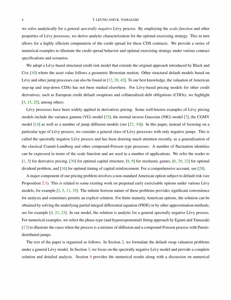
Theorem 3.1. The candidate function vB∗(x) is optimal for (2.14). Precisely,
vB∗(x) = v(x) = supτ∈S
Ex[e−rτh(Xτ )1τ<∞
],
and τ+B∗ is the optimal stopping time.

18 T. LEUNG AND K. YAMAZAKI
0 0.5 1 1.5 2 2.5 3-1
-0.8
-0.6
-0.4
-0.2
0
0.2
0.4
0.6
0.8
1
x
0 0.5 1 1.5 2 2.5 3-1
-0.8
-0.6
-0.4
-0.2
0
0.2
0.4
0.6
0.8
1
x
unbounded variation case bounded variation case
FIGURE 1. Illustrating the continuous and smooth fits of the value function vB∗(·) (solid curve)
and stopping value h(·) (dashed curve). Here vB∗(0+) = 0 for the unbounded variation case
while vB∗(0+) > 0 for the bounded variation case.
In order to verify the optimality of vB∗ , we shall show that (i) vB∗ dominates h and (ii) the stochastic process
Mt := e−r(t∧θ)vB∗(Xt∧θ), t ≥ 0(3.15)
is a supermartingale.
We address the first part as follows. When B∗ = 0, it is clear that vB∗(x) = h(x) from (2.21) or the arguments
above. On the other hand, when the smooth fit condition is met, i.e. B∗ ∈ (0,∞), %(B) is monotonically
increasing and attains 0 at B∗. Therefore, when B∗ > x, vB(x) is increasing in B for B ∈ [x,B∗] by (3.13).
Then, by continuous fit in Remark 3.2, for any arbitrarily fixed x, taking B = x, we have vB∗(x) ≥ vx(x) = h(x).
Moreover, vB∗(x) = h(x) on x ≤ B∗ by definition. Consequently, (i) holds.
Lemma 3.3. We have vB∗(x) ≥ h(x) for every x ∈ R.
We now pursue the supermartingale property of the process M in (3.15). Define generator L by
Lf(x) = cf ′(x) +1
2σ2f ′′(x) +
∫ ∞0
[f(x− z)− f(x) + f ′(x)z10<z<1
]Π(dz)
for the unbounded variation case and
Lf(x) = µf ′(x) +
∫ ∞0
[f(x− z)− f(x)] Π(dz)

AMERICAN STEP-UP AND STEP-DOWN CDS 19
for the bounded variation case. We shall show that (L − r)vB∗(x) ≤ 0 for every x ∈ (0,∞)\B∗, again by way
of the scale functions.
Lemma 3.4. Fix 0 < x ≤ B <∞. The stochastic processese−r(t∧τ
+B )W (r)(Xt∧τ+B
); t ≥ 0
ande−r(t∧τ
+B )Z(r)(Xt∧τ+B
); t ≥ 0
are Px-martingales.
The following is immediate by the previous lemma and the definition of vB∗ in (3.14).
Lemma 3.5. If 0 < B∗ <∞, then (L − r)vB∗(x) = 0 for every x ∈ (0, B∗).
Now we establish via the following lemmas that (L − r)vB∗(x) ≤ 0 for every x > B∗.
Lemma 3.6. If B∗ = 0, then we have (L − r)vB∗(0+) = (L − r)h(0+) ≤ 0.
Lemma 3.7. If 0 < B∗ <∞, then we have ∆′′(B∗−) ≥ 0.
Suppose 0 < B∗ < ∞. Since vB∗(·) and v′B∗(·) are continuous at B∗ by the continuous and smooth fit
conditions, it follows from Lemma 3.7 that (L − r)vB∗(B∗−) ≥ (L − r)vB∗(B∗+), and then by Lemma 3.5 that
(L − r)vB∗(B∗+) ≤ 0. Suppose B∗ = 0, we have (L − r)vB∗(B∗+) ≤ 0 by Lemma 3.6. Now, in order to show
(L − r)vB∗(x) ≤ 0 on (B∗,∞), it is sufficient to prove that (L − r)vB∗(x) is decreasing on (B∗,∞). Rewrite
vB∗ as in the following:
vB∗(x) =(h(x) + ∆(x)
)1x 6=0, x ∈ R
where
h(x) = −(p
r+ α
)(Z(r)(x)− r
Φ(r)W (r)(x)
), x ∈ R,
∆(x) =
(p
r+ α
)Z(r)(x)− W (r)(x)
W (r)(B∗)G(r)(B∗), x ∈ (−∞, B∗),
p
r− γ, x ∈ [B∗,∞).
(3.16)
Lemma 3.4 implies (L − r)h(x) = 0 for every x > 0. Furthermore, ∆′(x) = ∆′′(x) = 0 on x > B∗, and hence
(L − r)vB∗(x) = (L − r)∆(x) =
∫ ∞0
(∆(x− z)− ∆(x)
)Π(dz)− (p− rγ) , x > B∗.
In order to show that this is decreasing in x on (B∗,∞), it is sufficient to show that the integrand in the right-hand
side is decreasing in x or equivalently ∆(x − z) is decreasing in x for every fixed z by noting that ∆(x) is a
constant on (B∗,∞).

20 T. LEUNG AND K. YAMAZAKI
Lemma 3.8. The function ∆(·) is decreasing on R and is uniformly bounded below by p/r − γ > 0.
Therefore, we have (L − r)vB∗(x) ≤ 0 for every x > B∗, with 0 ≤ B∗ < ∞. Along with Lemma 3.5, we
conclude that
Lemma 3.9. The function vB∗(·) satisfies
(L − r)vB∗(x) ≤ 0, x ∈ (0,∞)\B∗.
Lemmas 3.3 and 3.9 prove the optimality. Due to the potential discontinuity of the value function at zero, care
must be taken in the proof. The rest of the proof is given in the appendix.
3.3. Putable Step-Down CDS. We now turn our attention to the putable step-down CDS, which amounts to
solving u(x) in (2.15) with p > 0 and α > 0. Under the spectrally negative Levy model, the function Γ(· ;A)
in (2.24) can be expressed explicitly by scale functions as shown in Lemma 3.10 below. This together with (3.4)
expresses explicitly ∆A(·) in (2.23), which is needed to apply continuous and smooth fit principle.
Define
ρ(A) :=
∫ ∞A
Π(du)(
1− e−Φ(r)(u−A)), A > 0.(3.17)
Here ρ(A) decreases monotonically in A because
ρ′(A) = −∫ ∞A
Π(du)Φ(r)e−Φ(r)(u−A) < 0.
Next, we express Γ(· ;A) using ρ(A) and the scale function.
Lemma 3.10. Fix A > 0, we have
Γ(x ;A) =1
Φ(r)W (r)(x−A)ρ(A)− 1
r
∫ ∞A
Π(du)(Z(r)(x−A)− Z(r)(x− u)
), for A ≤ x,
and Γ(x ;A) = 0 for x < A.
We proceed to consider the continuous fit condition. First, it follows from (2.23) that, for every A > 0,
∆A(A+) =
(γ +
p
r
)(r
Φ(r)W (r)(0)
)− (α− γ)
(1
Φ(r)W (r)(0)ρ(A)
)=W (r)(0)
Φ(r)((rγ + p)− (α− γ)ρ(A)) .
(3.18)

AMERICAN STEP-UP AND STEP-DOWN CDS 21
If X is of unbounded variation, then W (r)(0) = 0 by Lemma 3.1, and therefore continuous fit holds for every
A > 0. Nevertheless, for the bounded variation case, we can apply the continuous fit condition: ∆A(A+) = 0,
which is equivalent to
(α− γ)ρ(A) = (γr + p).(3.19)
For the unbounded variation case, we apply the smooth fit condition. By differentiation, we have
∂
∂xζ(x−A)
∣∣∣∣x=A+
= − r
Φ(r)W (r)′(0+) and
∂
∂xΓ(x;A)
∣∣∣∣x=A+
=ρ(A)
Φ(r)W (r)′(0+),
where W (r)′(0+) > 0 (in particular, W (r)′(0+) =∞ if σ = 0 and Π(0,∞) =∞ by Lemma 3.1). Therefore,
∆′A(A+) =W (r)′(0+)
Φ(r)((γr + p)− (α− γ)ρ(A)) .
Consequently, the smooth fit condition, ∆′A(A+) = 0, is equivalent to (3.19).
In summary, we look for the solution to (3.19), denoted by A∗, which will be our candidate optimal threshold.
Since ρ(A) is monotonically decreasing, there exists at most one A∗ that satisfies (3.19). If it does not exist, we
set the threshold A∗ = 0.
When X has paths of bounded variation, we must have A∗ > 0 under assumption (2.19). Indeed, if A∗ = 0,
then it follows from (3.18) that ∆A(A+) > 0 for every A > 0. This implies that there exists ε > 0 such that
uε(ε+) > g(0+). However, since g(0+) attains the global maximum (because g(0+) > 0 by (2.19)), this is a
contradiction. Hence A∗ = 0 is impossible when X is of unbounded variation.
In the case with A∗ > 0, we take A∗ to be our candidate optimal threshold, and the corresponding stopping time
is τ−A∗ . The candidate value function is given by
uA∗(x) =
g(x) + ∆A∗(x), x > A∗,
g(x), 0 < x ≤ A∗,
0, x ≤ 0.
For x > 0, we can apply (3.19) to express it as
uA∗(x) = (α− γ)
(1
r
∫ ∞A∗
Π(du)[Z(r)(x−A∗)− Z(r)(x− u)
])−(γ +
p
r
)Z(r)(x−A∗) +
(p
r+ α
)ζ(x).
(3.20)
22 T. LEUNG AND K. YAMAZAKI
When A∗ = 0, we consider the candidate value function defined by
uA∗(x) := limA↓0
uA(x)
= −(α− γ)Γ(x;A∗)−(γ +
p
r
)ζ(x−A∗) +
(p
r+ α
)ζ(x)
= (α− γ)(ζ(x)− Γ(x; 0))
(3.21)
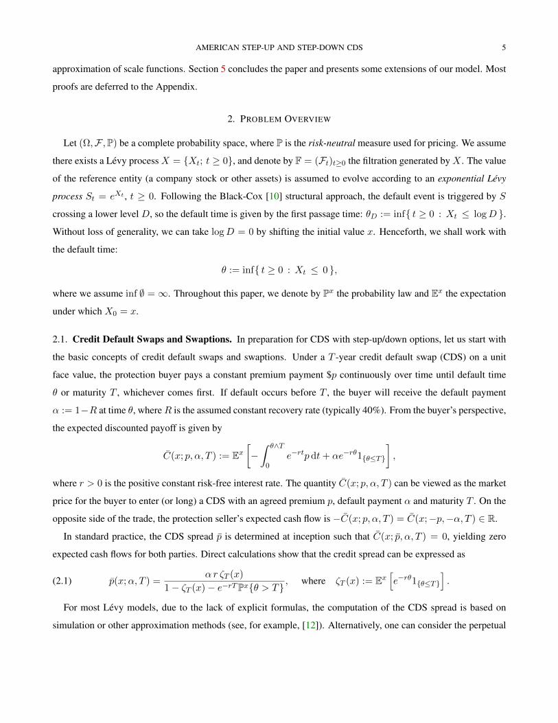
for all x > 0 and uA∗(x) = 0 for every x ≤ 0. This means that the seller will delay the exercise until X is
arbitrarily close to zero, by exercising at a sufficiently small level ε > 0. This can be realized by monitoring X as
it creeps downward through zero (see Section 5.3 of [28]). The seller may lose the opportunity to exercise prior to
default if X suddenly jumps across (below) zero.
0 0.5 1 1.5 2 2.5 3-0.4
-0.2
0
0.2
0.4
0.6
0.8
1
x
0 0.5 1 1.5 2 2.5 3-0.4
-0.2
0
0.2
0.4
0.6
0.8
1
x
unbounded variation case bounded variation case
FIGURE 2. Illustrating the continuous and smooth fits of the value function uA∗(·) (solid curve)
and stopping value g(·) (dashed curve). Here uA∗(·) is C1 at A∗ for the unbounded variation case
while it is C0 for the bounded variation case.
Theorem 3.2. The candidate function uA∗(x) is indeed optimal. That is,
uA∗(x) = u(x) = supτ∈S
Ex[e−rτg(Xτ )1τ<∞
].
Similarly to the previous subsection, we shall show (i) uA∗ ≥ g and (ii) the supermartingale property of the
value function. We shall first show the former.

AMERICAN STEP-UP AND STEP-DOWN CDS 23
Lemma 3.11. For every 0 < A < x, we have
∂
∂AuA(x) =
∂
∂A∆A(x) < 0 ⇐⇒ (α− γ)ρ(A)− (γr + p) < 0 ⇐⇒ A > A∗.
Suppose A∗ > 0. For the unbounded variation case, we can apply Lemma 3.11 for any fixed x ≥ A∗, along
with the continuous fit (which holds at any A), to get the inequality
uA∗(x) ≥ ux(x) = g(x), x ≥ A∗.
When X is of bounded variation, we have, by (3.18), ∆x(x+) ≥ 0 for every x ≥ A∗ and hence
uA∗(x) ≥ limA↑x
uA(x) = g(x) + limA↑x
∆A(x) ≥ g(x), x ≥ A∗.(3.22)
This also holds for the case A∗ = 0 by (3.21). Therefore, because uA∗(x) = g(x) on (−∞, A∗) by definition, we
have the following.
Lemma 3.12. We have uA∗(x) ≥ g(x) for every x ∈ R.
By taking advantage of Lemma 3.4 and how A∗ is chosen, we can show the following.
Lemma 3.13. We have (L − r)uA∗(x) ≤ 0 for every x ∈ (0,∞)\A∗.
Finally, Lemmas 3.12 and 3.13 show Theorem 3.2. The proof that uA∗ ≥ u can be carried out as in the proof
of Theorem 3.1. We also have uA∗ ≤ u. Indeed, uA∗ is attained by τ−A∗ when A∗ > 0 and can be approximated
arbitrarily closely by uε (attained by τ−ε ) for sufficiently small ε when A∗ = 0.
4. NUMERICAL EXAMPLES
In this section , we illustrate the investor’s optimal exercise strategy and the credit spread behaviors through a
series of numerical examples, where the underlying spectrally negative Levy process is assumed to have hyperex-
ponential jumps. The class of hyperexponential distributions is dense in the class of all positive-valued distributions
with completely monotone densities (see, e.g., [17, 19]). In a related work, Asmussen et al. [3] approximate the
Levy density of the CGMY process by a hyperexponential distribution.
4.1. Spectrally negative Levy processes with hyperexponential jumps. Let X be a spectrally negative Levy
process of the form
(4.1) Xt −X0 = µt+ σBt −Nt∑n=1
Zn, 0 ≤ t <∞.

24 T. LEUNG AND K. YAMAZAKI
Here B = Bt; t ≥ 0 is a standard Brownian motion, N = Nt; t ≥ 0 is a Poisson process with arrival rate
λ, and Z = Zn;n = 1, 2, . . . is an i.i.d. sequence of hyperexponential distributed random variables with density
function
f(z) =m∑i=1
αiηie−ηiz, z > 0,
for some 0 < η1 < · · · < ηm <∞. Its Laplace exponent (3.1) is then
ψ(s) = µs+1
2σ2s2 − λ
m∑i=1
αis
ηi + s.(4.2)
Notice in this case that −ηi; i = 1, . . . ,m are the poles of the Laplace exponent ψ. Here we assume σ > 0; for
the case with σ = 0, see [17].
In this case, there are m + 1 negative solutions to the equation ψ(s) = r and their absolute values ξi,r; i =
1, . . . ,m+ 1 satisfy the interlacing condition:
0 < ξ1,r < η1 < ξ2,r < · · · < ηm < ξm+1,r <∞.
The scale function becomes
W (r)(x) =2
σ2∑m+1
i=1 Ai,rξi,r
m+1∑i=1
Ai,r
(ξi,r
Φ(r) + ξi,r
)[eΦ(r)x − e−ξi,rx
],
Z(r)(x) = 1 +2r
σ2∑m+1
i=1 Ai,rξi,r
m+1∑i=1
Ai,r
(ξi,r
Φ(r) + ξi,r
)[1
Φ(r)
(eΦ(r)x − 1
)+
1
ξi,r
(e−ξi,rx − 1
)](4.3)
for every x ≥ 0 where
Ak,r :=
∏j∈1,...,m
(1− ξk,r
ηj
)∏i∈1,...,m\k
(1− ξk,r
ξi,r
) , 1 ≤ k ≤ m+ 1.
Note in this case that
WΦ(r)(x) =2
σ2∑m+1
i=1 Ai,rξi,r
m+1∑i=1
Ai,r
(ξi,r
Φ(r) + ξi,r
)[1− e−(Φ(r)+ξi,r)x
], x ≥ 0,
which is concave in x. Hence, Assumption 3.1 is satisfied. Furthermore, (3.17) becomes
ρ(A) = λm∑i=1
αiΦ(r)
ηi + Φ(r)e−ηiA, A > 0.

AMERICAN STEP-UP AND STEP-DOWN CDS 25
4.2. Hyperexponential Fitting. If a density function f(·) is completely monotone, then it can be approximated
arbitrarily closely by those of hyperexponential distributions. Consequently, as discussed in [17], the scale function
of any spectrally negative Levy process with a completely monotone Levy measure can be approximated in terms
of the scale functions defined in (4.3). Here we give an example using the results obtained by Feldmann and Whitt
[19] for the case Z in (4.1) is Pareto distributed.
The Pareto distribution with positive parameters a and b is given by
F (t) = 1− (1 + bt)−a, t ≥ 0.
These have long-tails, namely eδt(1− F (t)) → ∞ as t → ∞ for any δ > 0; see [24] for more details. Feldmann
and Whitt [19] introduced a recursive algorithm to fit hyperexponential distributions and specifically computed for
Pareto and Weibull distributions. We adopt their procedure for the process in the form (4.1) with Z replaced by
Pareto random variables with a = 1.2 and b = 5. Table 3 shows the fitted data. The corresponding scale functions
can be approximated by those in the form (4.3). For the convergence results, we refer to the author’s previous work
[17].
i αi ηi i αi ηi
1 8.37E-11 8.3E-09 8 0.000147 0.0020
2 7.18E-10 6.8E-08 9 0.001122 0.0100
3 5.56E-09 3.9E-07 10 0.008462 0.0570
4 4.27E-08 2.2E-06 11 0.059768 0.3060
5 3.27E-07 1.2E-05 12 0.307218 1.5460
6 2.50E-06 6.5E-05 13 0.533823 6.5160
7 1.92E-05 3.5E-04 14 0.089437 23.304
TABLE 3. Parameters of the hyperexponential distributions fitted to a Pareto distribution with
a = 1.2 and b = 5 (taken from Table 9 of Feldmann and Whitt [19]).
4.3. Numerical Results. Let us denote the step-up/down ratio by q := p/p = α/α. For both callable and putable
CDSs, we consider the following three cases:
(C) Cancellable CDS with q = 0,
(D) Step-Down CDS with q = 0.5,
(U) Step-Up CDS with q = 1.5.
26 T. LEUNG AND K. YAMAZAKI
Hence, there are in total 6 cases. The model parameters are r = 0.03 and σ = 0.2, α = 1, x = 1.5 and γ = 50bps,
unless specified otherwise. We shall adjust the values of λ and µ so that the risk-neutral condition ψ(1) = r is
satisfied.
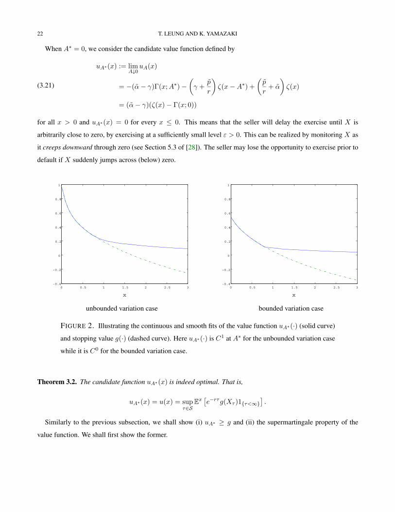
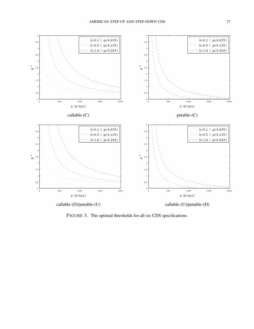
By the symmetry argument discussed in Section 2.4, the optimal stopping problems for callable-(D) CDS and
putable-(U) CDS are equivalent. The callable-(U) and putable-(D) CDSs are also equivalent. Figure 3 shows
the optimal thresholds B∗ for callable-(C), callable-(D) and putable-(U) CDSs, and also the optimal threshold A∗
for callable-(U), putable-(C) and putable-(D) CDSs. Both B∗ and A∗ are decreasing in the premium p. This is
intuitive: for callable-(C/D) CDS, the higher premium (cost to the protection buyer) induces the buyer to exercise
earlier at a lower level B∗ to cancel or step-down the position; in contrast, for the putable-(C/D) CDS, receiving
a higher premium motivates the protection seller to delay exercising to cancel or step-down by choosing a lower
exercise threshold A∗. Also, both A∗ and B∗ increase as λ increases because it raises the chance of down-crossing
the level zero. In particular, A∗ becomes zero when λ = 0.
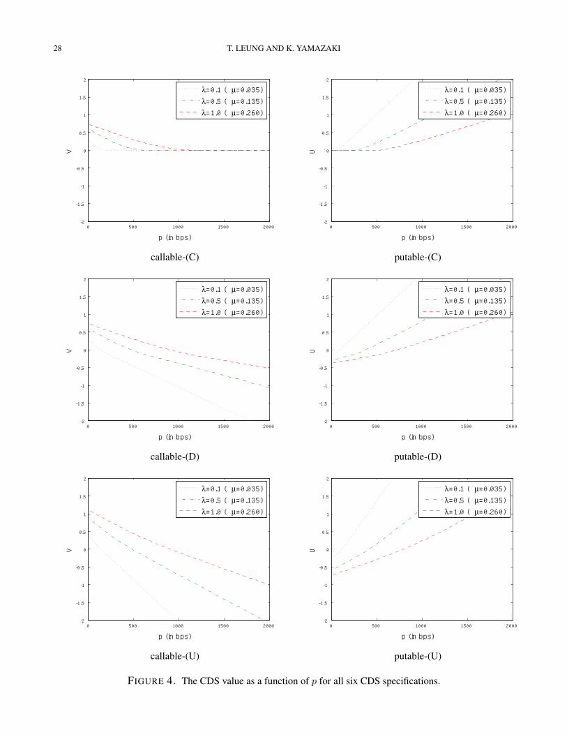
In Figure 4, we plot the CDS values V and U with respect to p (recall (2.8) and (2.12) for definitions). In
all cases, V is decreasing while U is increasing in p. For case (C), the values of V and U go to −γ when p is
sufficiently high and when it is sufficient low, respectively, because immediate stopping is optimal. For cases (D)
and (U), since the premium remains positive even after exercise, the value functions go to −∞ (for callable) and
∞ (for putable) as p increases. We also observe that, as λ increases, V increases and U decreases. Using the
functions V and U , the credit spread (or fair premiums) p∗ is determined where V (p∗) = 0 for the callable case,
and U(p∗) = 0 for the putable case.
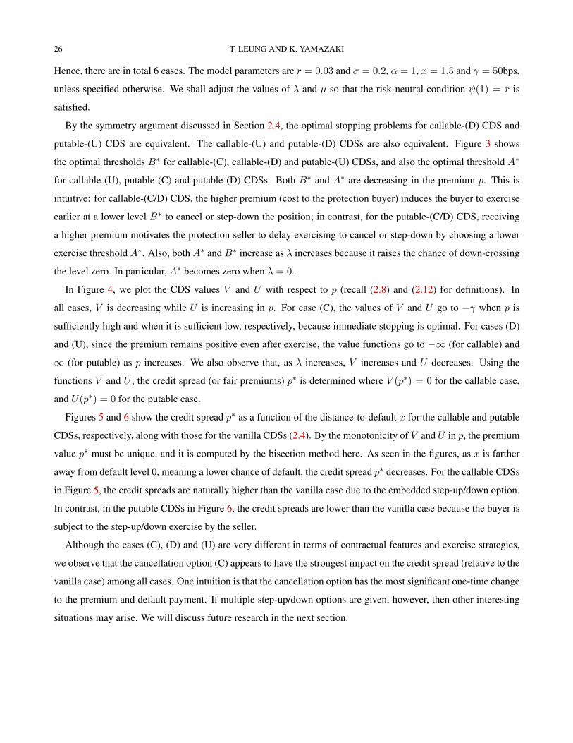
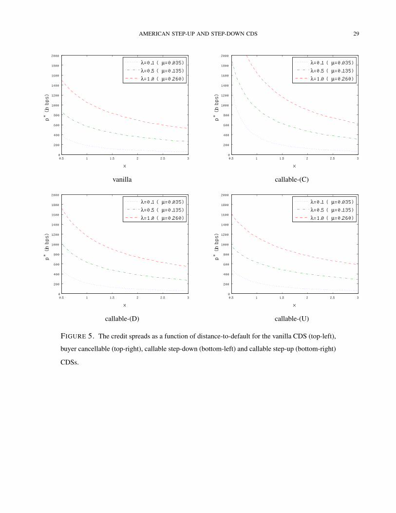
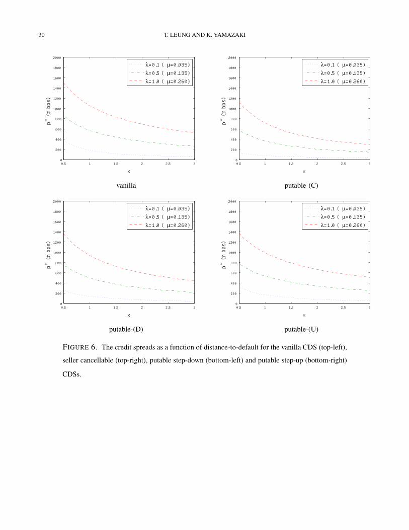
Figures 5 and 6 show the credit spread p∗ as a function of the distance-to-default x for the callable and putable
CDSs, respectively, along with those for the vanilla CDSs (2.4). By the monotonicity of V and U in p, the premium
value p∗ must be unique, and it is computed by the bisection method here. As seen in the figures, as x is farther
away from default level 0, meaning a lower chance of default, the credit spread p∗ decreases. For the callable CDSs
in Figure 5, the credit spreads are naturally higher than the vanilla case due to the embedded step-up/down option.
In contrast, in the putable CDSs in Figure 6, the credit spreads are lower than the vanilla case because the buyer is
subject to the step-up/down exercise by the seller.
Although the cases (C), (D) and (U) are very different in terms of contractual features and exercise strategies,
we observe that the cancellation option (C) appears to have the strongest impact on the credit spread (relative to the
vanilla case) among all cases. One intuition is that the cancellation option has the most significant one-time change
to the premium and default payment. If multiple step-up/down options are given, however, then other interesting
situations may arise. We will discuss future research in the next section.
AMERICAN STEP-UP AND STEP-DOWN CDS 27
0 500 1000 1500 20000
0.5
1
1.5
2
2.5
3
3.5
4
4.5
5B*
p (in bps)
λ=0.1 ( μ=0.035)λ=0.5 ( μ=0.135)λ=1.0 ( μ=0.260)
0 500 1000 1500 20000
0.5
1
1.5
2
2.5
3
3.5
4
4.5
5
A*
p (in bps)
λ=0.1 ( μ=0.035)λ=0.5 ( μ=0.135)λ=1.0 ( μ=0.260)
callable-(C) putable-(C)
0 500 1000 1500 20000
0.5
1
1.5
2
2.5
3
3.5
4
4.5
5
B*
p (in bps)
λ=0.1 ( μ=0.035)λ=0.5 ( μ=0.135)λ=1.0 ( μ=0.260)
0 500 1000 1500 20000
0.5
1
1.5
2
2.5
3
3.5
4
4.5
5
A*
p (in bps)
λ=0.1 ( μ=0.035)λ=0.5 ( μ=0.135)λ=1.0 ( μ=0.260)
callable-(D)/putable-(U) callable-(U)/putable-(D)
FIGURE 3. The optimal thresholds for all six CDS specifications.
28 T. LEUNG AND K. YAMAZAKI
0 500 1000 1500 2000-2
-1.5
-1
-0.5
0
0.5
1
1.5
2
V
p (in bps)
λ=0.1 ( μ=0.035)λ=0.5 ( μ=0.135)λ=1.0 ( μ=0.260)
0 500 1000 1500 2000-2
-1.5
-1
-0.5
0
0.5
1
1.5
2
U
p (in bps)
λ=0.1 ( μ=0.035)λ=0.5 ( μ=0.135)λ=1.0 ( μ=0.260)
callable-(C) putable-(C)
0 500 1000 1500 2000-2
-1.5
-1
-0.5
0
0.5
1
1.5
2
V
p (in bps)
λ=0.1 ( μ=0.035)λ=0.5 ( μ=0.135)λ=1.0 ( μ=0.260)
0 500 1000 1500 2000-2
-1.5
-1
-0.5
0
0.5
1
1.5
2
U
p (in bps)
λ=0.1 ( μ=0.035)λ=0.5 ( μ=0.135)λ=1.0 ( μ=0.260)
callable-(D) putable-(D)
0 500 1000 1500 2000-2
-1.5
-1
-0.5
0
0.5
1
1.5
2
V
p (in bps)
λ=0.1 ( μ=0.035)λ=0.5 ( μ=0.135)λ=1.0 ( μ=0.260)
0 500 1000 1500 2000-2
-1.5
-1
-0.5
0
0.5
1
1.5
2
U
p (in bps)
λ=0.1 ( μ=0.035)λ=0.5 ( μ=0.135)λ=1.0 ( μ=0.260)
callable-(U) putable-(U)
FIGURE 4. The CDS value as a function of p for all six CDS specifications.
AMERICAN STEP-UP AND STEP-DOWN CDS 29
0.5 1 1.5 2 2.5 30
200
400
600
800
1000
1200
1400
1600
1800
2000
p* (in bps)
x
λ=0.1 ( μ=0.035)λ=0.5 ( μ=0.135)λ=1.0 ( μ=0.260)
0.5 1 1.5 2 2.5 30
200
400
600
800
1000
1200
1400
1600
1800
2000
p* (in bps)
x
λ=0.1 ( μ=0.035)λ=0.5 ( μ=0.135)λ=1.0 ( μ=0.260)
vanilla callable-(C)
0.5 1 1.5 2 2.5 30
200
400
600
800
1000
1200
1400
1600
1800
2000
p* (in bps)
x
λ=0.1 ( μ=0.035)λ=0.5 ( μ=0.135)λ=1.0 ( μ=0.260)
0.5 1 1.5 2 2.5 30
200
400
600
800
1000
1200
1400
1600
1800
2000
p* (in bps)
x
λ=0.1 ( μ=0.035)λ=0.5 ( μ=0.135)λ=1.0 ( μ=0.260)
callable-(D) callable-(U)
FIGURE 5. The credit spreads as a function of distance-to-default for the vanilla CDS (top-left),
buyer cancellable (top-right), callable step-down (bottom-left) and callable step-up (bottom-right)
CDSs.
30 T. LEUNG AND K. YAMAZAKI
0.5 1 1.5 2 2.5 30
200
400
600
800
1000
1200
1400
1600
1800
2000
p* (in bps)
x
λ=0.1 ( μ=0.035)λ=0.5 ( μ=0.135)λ=1.0 ( μ=0.260)
0.5 1 1.5 2 2.5 30
200
400
600
800
1000
1200
1400
1600
1800
2000
p* (in bps)
x
λ=0.1 ( μ=0.035)λ=0.5 ( μ=0.135)λ=1.0 ( μ=0.260)
vanilla putable-(C)
0.5 1 1.5 2 2.5 30
200
400
600
800
1000
1200
1400
1600
1800
2000
p* (in bps)
x
λ=0.1 ( μ=0.035)λ=0.5 ( μ=0.135)λ=1.0 ( μ=0.260)
0.5 1 1.5 2 2.5 30
200
400
600
800
1000
1200
1400
1600
1800
2000
p* (in bps)
x
λ=0.1 ( μ=0.035)λ=0.5 ( μ=0.135)λ=1.0 ( μ=0.260)
putable-(D) putable-(U)
FIGURE 6. The credit spreads as a function of distance-to-default for the vanilla CDS (top-left),
seller cancellable (top-right), putable step-down (bottom-left) and putable step-up (bottom-right)
CDSs.
AMERICAN STEP-UP AND STEP-DOWN CDS 31
5. CONCLUDING REMARKS
In summary, the incorporation of American step-up and step-down options give CDS investors the additional
flexibility to manage and trade credit risks. The valuation of these contracts requires solving for the optimal timing
to step-up/down for the protection buyer/seller. The perpetual nature of the contract allows us to compute analyt-
ically the investor’s optimal exercise threshold under quite general Levy credit risk models. Using the symmetry
properties between step-up and step-down contracts, we gain better intuition on various contract specifications,
and drastically simplify the procedure to determine the credit spreads.
There are a number of avenues for future research. For instance, it would be interesting to value a CDS where
both the protection buyer and seller can terminate the contract early. Then, the valuation problem can be formulated
as a modified game option as introduced by Kifer [26]. In this case, we conjecture that threshold strategies will
again be optimal for both parties and constitute Nash or Stackelberg equilibrium [18, 37]. Another direction for
future research is to consider derivatives with multiple early exercisable step-up/down options. This is related to
some optimal multiple stopping problems arising in other financial applications, such as swing options [13] and
employee stock options [31].
APPENDIX A. PROOFS
A.1. Proofs for Section 2.
Proof of Lemma 2.1. Applying the definitions of ∆B(x) and h(x) (see (2.11)) and noting that θ = ∞ whenever
τ+B =∞, we obtain, for every x ∈ (0, B),
∆B(x)
= Ex[
1τ+B<∞
(∫ θ
τ+B
e−rtp dt− e−rτ+B γ1τ+B<θ
− e−rθα1τ+B<θ
)]− Ex
[∫ θ
0e−rtp dt − e−rθα
]+ γ
= Ex[
1τ+B<∞
(−∫ τ+B
0e−rtp dt− e−rτ
+B γ1τ+B<θ
+ e−rθα1τ+B=θ
)− 1τ+B=∞
(∫ θ
0e−rtp dt − e−rθα
)]+ γ
= Ex[
1τ+B<∞e−rτ
+B
(α1τ+B=θ − γ1τ+B<θ
)−
(∫ τ+B
0e−rtpdt
)]+ γ
= Ex[1τ+B<∞
e−rτ+B
((p
r+ α
)1τ+B=θ +
(p
r− γ)
1τ+B<θ
)]+ γ − p
r.

32 T. LEUNG AND K. YAMAZAKI
Proof of Lemma 2.2. Using the same argument as in the proof of Lemma 2.1, we can write
∆A(x) =
(p
r+ γ
)− Ex
[e−rτ
−A
((α+
p
r
)1τ−A=θ,τ−A<∞
+
(γ +
p
r
)1τ−A<θ,τ
−A<∞
)].
Therefore, we have
∆A(x) =
(p
r+ γ
)− Ex
[e−rτ
−A
((γ +
p
r
)1τ−A<∞
+ (α− γ)1τ−A=θ,τ−A<∞
)]=
(γ +
p
r
)(1− ζ(x−A))− (α− γ)Γ(x;A).
A.2. Proofs for Subsection 3.2.
Proof of Lemma 3.2. When σ > 0 or Π(0,∞) = ∞, we have %(0+) = −∞ because W (r)′(0+) > 0 and
W (r)(0) = 0 by Lemma 3.1. This implies that both (1) and (2) are necessary conditions for B∗ = 0. Now suppose
(1) and (2). Again by Lemma 3.1 we have after some algebra
%(0+) =1
µ(p− rγ − (α+ γ)Π(0,∞)) .
Therefore, condition (3) implies that %(·) ≥ 0 (i.e. scenario (a)) since %(·) is increasing. The proof is complete.
Proof of Lemma 3.4. By (3.3) and strong Markov property, we write
Ex[e−rτ
+B 1τ+B<θ
∣∣∣Ft∧τ+B ] = e−r(t∧τ+B )W (r)(Xt∧τ+B
)
W (r)(B), t ≥ 0.
Therefore, by taking expectation on both sides, we obtain
Ex[e−r(t∧τ
+B )W (r)(Xt∧τ+B
)
W (r)(B)
]= Ex
[e−rτ
+B 1τ+B<θ
]=W (r)(x)
W (r)(B), t ≥ 0.
Hence
Ex[e−r(t∧τ
+B )W (r)(Xt∧τ+B
)]
= W (r)(x), t ≥ 0.
Furthermore, we have the bound 0 ≤W (r)(Xt∧τ+B) ≤W (r)(B). This shows the first claim.
Similarly, (3.3) and strong Markov property yield that
Ex[e−rτ
+B 1τ+B=θ
∣∣∣Ft∧τ+B ] = e−r(t∧τ+B )
(Z(r)(Xt∧τ+B
)− r
Φ(r)W (r)(Xt∧τ+B
)
), t ≥ 0.
By taking expectation on both sides, we get
Ex[e−r(t∧τ
+B )
(Z(r)(Xt∧τ+B
)− r
Φ(r)W (r)(Xt∧τ+B
)
)]= Ex
[e−rτ
+B 1τ+B=θ
]= Z(r)(x)− r
Φ(r)W (r)(x).
With this and the bound 1 ≤ Z(r)(Xt∧τ+B) ≤ Z(r)(B), we conclude the second claim.

AMERICAN STEP-UP AND STEP-DOWN CDS 33
Proof of Lemma 3.6. By using the martingale property of Lemma 3.4, we have
(L − r)h(0+) = (L − r)L(0+),
where
L(x) :=
(p
r− γ)
+ (α+ γ) 1x≤0, x ∈ R.
Now, with L′(0+) = 0 and σ = 0 and Π(0,∞) <∞ by Lemma 3.2, we obtain
(L − r)L(0+) =
∫ ∞0
(L(0− z)− L(0)) Π(dz)− r(p
r− γ)
= (α+ γ)Π(0,∞)− (p− γr) .
Hence, (L − r)h(0+) ≤ 0 by Lemma 3.2.
Proof of Lemma 3.7. Notice that
∆′′(B∗−) = (rα+ p)W (r)′(B∗)− W (r)′′(B∗)
W (r)(B∗)G(r)(B∗).
By (3.12), we have
G(r)(B∗) =
(W (r)(B∗)
)2W (r)′(B∗)
(p+ αr) .(A.1)
Direction substitution yields that
∆′′(B∗−) = (rα+ p)1
W (r)′(B∗)
[(W (r)′(B∗)
)2−W (r)′′(B∗)W (r)(B∗)
]= − (rα+ p)
(W (r)(B∗))2
W (r)′(B∗)
∂
∂B
W (r)′(B)
W (r)(B),
which is non-negative by Assumption 3.1, as desired.
Proof of Lemma 3.8. It is clear that ∆(·) in (3.16) is monotonically decreasing when B∗ = 0 because ∆(0−) =
pr + α > p
r − γ = ∆(0+). Suppose 0 < B∗ <∞. By differentiating ∆(·), we get
∆′(x) = (p+ αr)W (r)(x)− W (r)′(x)
W (r)(B∗)G(r)(B∗)
= W (r)′(x)
(rα+ p)
[W (r)(x)
W (r)′(x)− W (r)(B∗)
W (r)′(B∗)
], 0 < x < B∗,
where the last equation follows from (A.1).
Now, ∆′(·) is non-positive because Assumption 3.1 implies that
W (r)′(x)
W (r)(x)≥ W (r)′(B∗)
W (r)(B∗)⇐⇒ W (r)(x)
W (r)′(x)≤ W (r)(B∗)
W (r)′(B∗), x ≤ B∗.

34 T. LEUNG AND K. YAMAZAKI
Furthermore, we note that
∆(0+)− ∆(0−) = − W (r)(0)
W (r)(B∗)G(r)(B∗) ≤ 0.
Finally, it follows from continuous fit that ∆(B∗−) = ∆(B∗+) = pr − γ > 0 (see (2.18)). This completes the
proof because ∆ is constant on (−∞, 0) ∪ (B∗,∞).
Proof of Theorem 3.1. Due to the potential discontinuity of the value function at zero, we need to proceed carefully.
Before showing the main result, we first prove that 0 = vB∗(0) ≤ vB∗(0+) as illustrated in Figure 1.
Suppose 0 < B∗ < ∞. Both h(x) and vB∗(x) are both increasing in x (see (2.16) and (3.14)). Since W (r) is
increasing and non-negative, we must have
p+ αr
Φ(r)− G(r)(B∗)
W (r)(B∗)≥ 0.
Therefore,
vB∗(0+) = W (r)(0)
(p+ αr
Φ(r)− G(r)(B∗)
W (r)(B∗)
)≥ 0,
and this is strictly positive if and only if X has paths of bounded variation by Lemma 3.1. On the other hand, if
B∗ = 0, we also have vB∗(0+) ≥ 0 because (3.13) implies that, for any ε > 0, ∂vB(ε)/∂B ≤ 0 for every B > ε
and limB→∞ vB(ε) = 0.
We now prove the optimality. We first construct a sequence of functions vn(·) such that (1) it is C2 everywhere
except at B∗, (2) vn(x) = vB∗(x) on x ∈ (0,∞) and (3) vn(x) ↓ vB∗(x) pointwise for every fixed x ∈ (−∞, 0).
This implies, by noting that v′B∗(x) = v′n(x) and v′′B∗(x) = v′′n(x) on (0,∞)\B∗, that (L − r)(vn − vB∗)(x)
decreases monotonically in n to zero for every fixed x ∈ (0,∞)\B∗ by monotone convergence theorem. Notice
that vB∗(·) is uniformly bounded because h(·) is. Hence, we can choose so that vn is also uniformly bounded for
every fixed n ≥ 1.
Notice that
Ex[∫ ν
0e−rs((L − r)vn(Xs))ds
]≤ Ex
[∫ ν
0e−rs((L − r)(vn − vB∗)(Xs))ds
]<∞, ν ∈ S.(A.2)
To see this, we have by Lemma 3.9
Ex[∫ ν
0e−rs((L − r)vn(Xs))ds
]= Ex
[∫ ν
0e−rs((L − r)vB∗(Xs))ds
]+Ex
[∫ ν
0e−rs((L − r)(vn − vB∗)(Xs))ds
]≤ Ex
[∫ ν
0e−rs((L − r)(vn − vB∗)(Xs))ds
]≤ KEx
[∫ θ
0e−rsΠ(Xs,∞)ds
]

AMERICAN STEP-UP AND STEP-DOWN CDS 35
where K <∞ is the maximum difference between vB∗ and vn. Using N as the Poisson random measure for −X ,
we have by compensation formula (see, e.g., Theorem 4.4 in [28])
Ex[∫ θ
0e−rsΠ(Xs,∞)ds
]= Ex
[∫ ∞0
∫ ∞0
e−rs1θ≥s, u>Xs−Π(du)ds
]= Ex
[∫ ∞0
∫ ∞0
e−rs1θ≥s, u>Xs−N(du× ds)
]= Ex
[e−rθ
]<∞.
Notice that, although vn is notC2 atB∗, the Lebesque measure of vn at whichX = B∗ is zero and hence v′′n(B∗)
can be chosen arbitrarily for the unbounded variation case. By applying Ito’s formula toe−r(t∧θ)vn(Xt∧θ); t ≥ 0
,
we see that e−r(t∧θ)vn(Xt∧θ)−
∫ t∧θ
0e−rs ((L − r)vn(Xs)) ds; t ≥ 0
(A.3)
is a local martingale. Suppose σk; k ≥ 1 is the corresponding localizing sequence, namely,
Ex[e−r(t∧θ∧σk)vn(Xt∧θ∧σk)
]= vn(x) + Ex
[∫ t∧θ∧σk
0e−rs ((L − r)vn(Xs)) ds
], k ≥ 1.
Now by applying dominated convergence theorem on the left-hand side and Fatou’s lemma on the right-hand side
via (A.2), we obtain
Ex[e−r(t∧θ)vn(Xt∧θ)
]≤ vn(x) + Ex
[∫ t∧θ
0e−rs ((L − r)vn(Xs)) ds
].
Hence, (A.3) is in fact a supermartingale.
Now fix ν ∈ S. By optional sampling theorem, we have, for any M ≥ 0, that
Ex[e−r(ν∧M)vn(Xν∧M )
]≤ vn(x) + Ex
[∫ ν∧M
0e−rs ((L − r)vn(Xs)) ds
]= vn(x) + Ex
[∫ ν∧M
0e−rs ((L − r)vB∗(Xs)) ds
]+ Ex
[∫ ν∧M
0e−rs ((L − r)(vn − vB∗)(Xs)) ds
]where the last equality holds because the expectation can be split by (A.2). Applying dominated convergence
theorem on the left-hand side and monotone convergence convergence theorem on the right-hand side (here the
integrands in the two expectations are negative and positive, respectively), along with Lemma 3.9, we obtain
Ex[e−rνvn(Xν)
]≤ vn(x) + Ex
[∫ ν
0e−rs((L − r)(vn − vB∗)(Xs))ds
].(A.4)
Furthermore, monotone convergence theorem yields the followings:
limn→∞
Ex[e−rνvn(Xν)
]= Ex
[e−rνvB∗(Xν)
],
limn→∞
Ex[∫ ν
0e−rs((L − r)(vn − vB∗)(Xs))ds
]= 0.

36 T. LEUNG AND K. YAMAZAKI
Therefore, by taking n→∞ on both sides of (A.4) (note vB∗(x) = vn(x)), we have
vB∗(x) ≥ Ex[e−rνvB∗(Xν)
]≥ Ex
[e−rνh(Xν)
], ν ∈ S,
where the last inequality follows from Lemma 3.3. This together with the fact that the stopping time τ+B∗ corre-
sponds to the value function vB∗ completes the proof of Theorem 3.1.
A.3. Proofs for Subsection 3.3.
Proof of Lemma 3.10. Let N be the Poisson random measure for −X . By the compensation formula, we get
Γ(x;A) = Ex[∫ ∞
0
∫ ∞0
N(dt× du)e−rt1τ−A≥t, Xt−−u<0
]= Ex
[∫ ∞0
dte−rt∫ ∞
0Π(du)1τ−A≥t, Xt−−u<0
]=
∫ ∞0
Π(du)
∫ ∞0
dt[e−rtPxXt− < u, τ−A ≥ t
].
Recall, for example from p.225 of [28], the fact∫ ∞0
dt[e−rtPx
Xt ∈ dy, τ−0 > t
]= dy
[e−Φ(r)yW (r)(x)−W (r)(x− y)
], y ≥ 0.
Applying this yields∫ ∞0
dt[e−rtPx
Xt ∈ dy, τ−A > t
]=
∫ ∞0
dt[e−rtPx−A
Xt ∈ d(y −A), τ−0 > t
]= dy
[e−Φ(r)(y−A)W (r)(x−A)−W (r)(x− y)
],
when y ≥ A, and it is 0 otherwise. Therefore, for u ≥ A, we have∫ ∞0
dt[e−rtPxXt− < u, τ−A ≥ t
]=
∫ u
Ady[e−Φ(r)(y−A)W (r)(x−A)−W (r)(x− y)
]=
∫ u−A
0dz[e−Φ(r)zW (r)(x−A)−W (r)(x− z −A)
]=W (r)(x−A)
Φ(r)
[1− e−Φ(r)(u−A)
]−∫ u−A
0dzW (r)(x− z −A),
and it is 0 on 0 ≤ u ≤ A. Substituting this back into Γ(x;A) above, we obtain
Γ(x;A) =
∫ ∞A
Π(du)
1
Φ(r)W (r)(x−A)
(1− e−Φ(r)(u−A)
)−∫ u−A
0dzW (r)(x−A− z)
.

AMERICAN STEP-UP AND STEP-DOWN CDS 37
Next, we apply (3.17) and that W (r)(x) = 0 and Z(r)(x) = 1 on (−∞, 0) to get
Γ(x;A)
=1
Φ(r)W (r)(x−A)ρ(A)−
∫ x
AΠ(du)
∫ u−A
0dzW (r)(x−A− z)−
∫ ∞x
Π(du)
∫ x−A
0dzW (r)(x−A− z)
=1
Φ(r)W (r)(x−A)ρ(A)− 1
r
∫ x
AΠ(du)
(Z(r)(x−A)− Z(r)(x− u)
)− 1
r
∫ ∞x
Π(du)(Z(r)(x−A)− 1
)=
1
Φ(r)W (r)(x−A)ρ(A)− 1
r
∫ ∞A
Π(du)(Z(r)(x−A)− Z(r)(x− u)
),
as desired.
Proof of Lemma 3.11. Fix A > 0. We differentiate to get
∂
∂Aζ(x−A) = −rW (r)(x−A) +
r
Φ(r)W (r)′(x−A),
∂
∂AΓ(x;A) = −ρ(A)
Φ(r)W (r)′(x−A) +W (r)(x−A)
∫ ∞A
Π(du)(
1− e−Φ(r)(u−A))
=
(W (r)(x−A)− 1
Φ(r)W (r)′(x−A)
)ρ(A).
Therefore, it follows from (2.23) that
∂
∂A∆A(x) =
(W (r)(x−A)− 1
Φ(r)W (r)′(x−A)
)((γr + p)− (α− γ)ρ(A)) .
Applying (3.6), we have the expressions
W (r)(x−A) = eΦ(r)(x−A)WΦ(r)(x−A),
W (r)′(x−A) = Φ(r)W (r)(x−A) + eΦ(r)(x−A)W ′Φ(r)(x−A),
which yield
∂
∂A∆A(x) =
eΦ(r)(x−A)
Φ(r)W ′Φ(r)(x−A) ((α− γ)ρ(A)− (γr + p)) .
This completes the proof because it is known that W ′Φ(r)(x−A) is positive and ρ(A) is decreasing.
Proof of Lemma 3.13. (1) We first show (L − r)uA∗(x) = 0 for every x > A∗. Let u be defined by (3.20) and
(3.21) on the whole real line (while uA∗(x) = 0 on x ∈ (−∞, 0]). Suppose A∗ > 0. Using (3.20) and recalling

38 T. LEUNG AND K. YAMAZAKI
that (L − r)Z(r)(y) = 0 and (L − r)W (r)(y) = 0 for every y > 0, we have
(L − r)u(x) = (α− γ)
[1
r
∫ ∞A∗
Π(du)[(L − r)Z(r)(x−A∗)− (L − r)Z(r)(x− u)
]]−(γ +
p
r
)(L − r)Z(r)(x−A∗) +
(p
r+ α
)[(L − r)Z(r)(x)− q
Φ(r)(L − r)W (r)(x)
]= −(α− γ)
[1
r
∫ ∞x
Π(du)[(L − r)Z(r)(x− u)
]]= (α− γ)Π(x,∞).
Suppose A∗ = 0. By (3.21), we obtain (L− r)u(x) = (α− γ)Π(x,∞) similarly to the case above. Furthermore,
it is easy to show that
(L − r)(uA∗(x)− u(x)) = −Π(x,∞)(α− γ),
and hence the proof is complete.
(2) We now show for the case A∗ > 0 that we have (L − r)uA∗(x) > 0 for every 0 < x < A∗. Notice that
uA∗(x) = g(x) on 0 < x < A∗. We have
(L − r)uA∗(x) = (L − r)L(x) where L(x) := −(γ +
p
r
)− (α− γ)1x≤0.
Therefore, we have
(L − r)uA∗(x) = (L − r)L(x) =
∫ ∞0
(L(x− u)− L(x)) Π(du)− rL(x)
= − (α− γ) Π(x,∞) + (rγ + p) ≤ − (α− γ) ρ(A∗) + (rγ + p) = 0.
Here the inequality holds by (3.17) and because x < A∗. The last equality holds by (3.19).
REFERENCES
[1] L. Alili and A. E. Kyprianou. Some remarks on first passage of Levy processes, the American put and pastingprinciples. Ann. Appl. Probab., 15(3):2062–2080, 2005.
[2] S. Asmussen, F. Avram, and M. R. Pistorius. Russian and American put options under exponential phase-typeLevy models. Stochastic Process. Appl., 109(1):79–111, 2004.
[3] S. Asmussen, D. Madan, and M. Pistorius. Pricing equity default swaps under an approximation to the CGMYlevy model. Journal of Computational Finance, 11(2):79–93, 2007.
[4] F. Avram, T. Chan, and M. Usabel. On the valuation of constant barrier options under spectrally one-sidedexponential Levy models and Carr’s approximation for American puts. Stochastic processes and applications,100:75–107, 2002.
[5] F. Avram, A. E. Kyprianou, and M. R. Pistorius. Exit problems for spectrally negative Levy processes andapplications to (Canadized) Russian options. Ann. Appl. Probab., 14(1):215–238, 2004.
AMERICAN STEP-UP AND STEP-DOWN CDS 39
[6] F. Avram, Z. Palmowski, and M. R. Pistorius. On the optimal dividend problem for a spectrally negative Levyprocess. Ann. Appl. Probab., 17(1):156–180, 2007.
[7] O. E. Barndorff-Nielsen. Processes of normal inverse Gaussian type. Finance Stoch., 2(1):41–68, 1998.[8] E. Baurdoux and A. E. Kyprianou. The McKean stochastic game driven by a spectrally negative Levy process.
Electron. J. Probab., 13:no. 8, 173–197, 2008.[9] E. Baurdoux and A. E. Kyprianou. The Shepp-Shiryaev stochastic game driven by a spectrally negative levy
process. Theory of Probability and Its Applications, 53, 2009.[10] F. Black and J. Cox. Valuing corporate securities: Some effects of bond indenture provisions. Journal of
Finance, 31:351–367, 1976.[11] S. Boyarchenko. Perpetual american options under Levy processes. SIAM Journal of Control and Optimiza-
tion, 40(6):1663 – 1696, 2002.[12] J. Cariboni and W. Schoutens. Pricing credit default swaps under Levy models. Journal of Computational
Finance, 10(4):1–21, 2007.[13] R. Carmona and N. Touzi. Optimal multiple stopping and valuation of swing options. Mathematical Finance,
18(2):239–268, April 2008.[14] P. Carr, H. Geman, D. B. Madan, and M. Yor. The fine structure of asset returns: An empirical investigation.
Journal of Business, 75(2):305–332, 2002.[15] E. Eberlein, W. Kluge, and P. J. Schonbucher. The Levy Libor model with default risk. Journal of Credit
Risk, 2(2):3–42, 2006.[16] M. Egami and K. Yamazaki. Precautionary measures for credit risk management in jump models. Discussion
Papers at Kyoto University and Osaka University, 2010.[17] M. Egami and K. Yamazaki. Solving optimal dividend problems via phase-type fitting approximation of scale
functions. Discussion Paper at Osaka University, 2010.[18] E. Ekstrom and G. Peskir. Optimal stopping games for Markov processes. SIAM J. Control Optim.,
47(2):684–702, 2008.[19] A. Feldmann and W. Whitt. Fitting mixtures of exponentials to long-tail distributions to analyze network
performance models. Performance Evaluation, (31):245–279, 1998.[20] B. Hilberink and C. Rogers. Optimal capital structure and endogenous default. Finance and Stochastics,
6(2):237–263, 2002.[21] A. Hirsa and D. Madan. Pricing american options under variance gamma. Journal of Computational Finance,
7(2), 2003.[22] J. Hull and A. White. The valuation of credit default swap options. Journal of Derivatives, 10(3):40–50,
2003.[23] K. Jackson, S. Jaimungal, and V. Surkov. Fourier space time stepping for option pricing with Levy models.
Journal of Computational Finance, 12(2):1–29, 2008.[24] N. L. Johnson and S. Kotz. Distributions in statistics: continuous multivariate distributions. John Wiley &
Sons Inc., New York, 1972. Wiley Series in Probability and Mathematical Statistics.[25] H. Josson and W. Schoutens. Single name credit default swaptions meet single sided jump models. Review
of Derivatives Research, 11(1):153–169, 2008.[26] Y. Kifer. Game options. Finance and Stochastics, 4:443–463, 2000.[27] S. G. Kou and H. Wang. Option pricing under a double exponential jump diffusion model. Manage. Sci.,
50(9):1178–1192, 2004.

40 T. LEUNG AND K. YAMAZAKI
[28] A. E. Kyprianou. Introductory lectures on fluctuations of Levy processes with applications. Universitext.Springer-Verlag, Berlin, 2006.
[29] A. E. Kyprianou and Z. Palmowski. Distributional study of de Finetti’s dividend problem for a general Levyinsurance risk process. J. Appl. Probab., 44(2):428–448, 2007.
[30] A. E. Kyprianou and B. A. Surya. Principles of smooth and continuous fit in the determination of endogenousbankruptcy levels. Finance Stoch., 11(1):131–152, 2007.
[31] T. Leung and R. Sircar. Accounting for risk aversion, vesting, job termination risk and multiple exercises invaluation of employee stock options. Mathematical Finance, 19(1):99–128, January 2009.
[32] R. L. Loeffen. On optimality of the barrier strategy in de Finetti’s dividend problem for spectrally negativeLevy processes. Ann. Appl. Probab., 18(5):1669–1680, 2008.
[33] D. B. Madan, P. Carr, and E. Chang. The variance gamma process and option pricing. European FinanceReview, 2:79105, 1998.
[34] R. Merton. Option pricing when underlying stock returns are discontinuous. J. Financial Econom, 3:125–144,1976.
[35] E. Mordecki. Optimal stopping and perpetual options for Levy processes. Finance and Stochastics, 6:473–493, 2002.
[36] G. Peskir. Principles of optimal stopping and free-boundary problems, volume 68 of Lecture Notes Series(Aarhus). University of Aarhus, Department of Mathematics, Aarhus, 2001. Dissertation, University ofAarhus, Aarhus, 2002.
[37] G. Peskir. Optimal stopping games and Nash equilibrium. Theory Probab. Appl., 53(3):558–571, 2009.[38] G. Peskir and A. Shiryaev. Optimal stopping and free-boundary problems. Lectures in Mathematics ETH
Zurich. Birkhauser Verlag, Basel, 2006.[39] G. Peskir and A. N. Shiryaev. Sequential testing problems for Poisson processes. Ann. Statist., 28(3):837–
859, 2000.[40] G. Peskir and A. N. Shiryaev. Solving the Poisson disorder problem. In Advances in finance and stochastics,
pages 295–312. Springer, Berlin, 2002.[41] B. A. Surya. Evaluating scale functions of spectrally negative Levy processes. J. Appl. Probab., 45(1):135–
149, 2008.[42] C. Zhou. The term structure of credit spreads with jump risk. Journal of Banking and Finance, 25:2015–2040,
2001.
Related Documents