AMath 483/583 — Lecture 23 Outline: • Linear systems: LU factorization and condition number • Heat equation and discretization • Iterative methods Sample codes: • $UWHPSC/codes/openmp/jacobi1d_omp1.f90 • $UWHPSC/codes/openmp/jacobi1d_omp2.f90 R.J. LeVeque, University of Washington AMath 483/583, Lecture 23

Welcome message from author
This document is posted to help you gain knowledge. Please leave a comment to let me know what you think about it! Share it to your friends and learn new things together.
Transcript

AMath 483/583 — Lecture 23
Outline:
• Linear systems: LU factorization and condition number• Heat equation and discretization• Iterative methods
Sample codes:
• $UWHPSC/codes/openmp/jacobi1d_omp1.f90
• $UWHPSC/codes/openmp/jacobi1d_omp2.f90
R.J. LeVeque, University of Washington AMath 483/583, Lecture 23

Announcements
Homework 6 is in the notes and due next Friday.
Quizzes for this week’s lectures due next Wednesday.
Office hours today 9:30 – 10:20.
Next week:
Monday: no class
Wednesday: Guest lecture —
Brad Chamberlain, Cray
Chapel: A Next-Generation PartitionedGlobal Address Space (PGAS) Language
R.J. LeVeque, University of Washington AMath 483/583, Lecture 23

AMath 483/583 — Lecture 23
Outline:
• Linear systems: LU factorization and condition number• Heat equation and discretization• Iterative methods
Sample codes:
• $UWHPSC/codes/openmp/jacobi1d_omp1.f90
• $UWHPSC/codes/openmp/jacobi1d_omp2.f90
R.J. LeVeque, University of Washington AMath 483/583, Lecture 23

DGESV — Solves a general linear system
SUBROUTINE DGESV( N, NRHS, A, LDA, IPIV,& B, LDB, INFO )
NRHS = number of right hand sides
B = matrix whose columns are right hand side(s) on inputsolution vector(s) on output.
LDB = leading dimension of B.
INFO = integer returning 0 if successful.
A = matrix on input, L,U factors on output,
IPIV = Returns pivot vector (permutation of rows)integer, dimension(N)Row I was interchanged with row IPIV(I).
R.J. LeVeque, University of Washington AMath 483/583, Lecture 23

Gaussian elimination as factorization
If A is nonsingular it can be factored as
PA = LU
where
P is a permutation matrix (rows of identity permuted),
L is lower triangular with 1’s on diagonal,
U is upper triangular.
After returning from dgesv:A contains L and U (without the diagonal of L),IPIV gives ordering of rows in P .
R.J. LeVeque, University of Washington AMath 483/583, Lecture 23

Gaussian elimination as factorization
Example:
A =
2 1 34 3 62 3 4
0 1 0
0 0 11 0 0
2 1 34 3 62 3 4
=
1 0 01/2 1 01/2 −1/3 1
4 3 60 1.5 10 0 1/3
IPIV = (2,3,1)
and A comes back from DGESV as: 4 3 61/2 1.5 11/2 −1/3 1/3
R.J. LeVeque, University of Washington AMath 483/583, Lecture 23

dgesv examples
See $UWHPSC/codes/lapack/random.
Sample codes that solve the linear system Ax = b with arandom n× n matrix A, where the value n is run-time input.
randomsys1.f90 is with static array allocation.
randomsys2.f90 is with dynamic array allocation.
randomsys3.f90 also estimates condition number of A.
κ(A) = ‖A‖ ‖A−1‖
Can bound relative error in solution in terms of relative error indata using this:
Ax∗ = b∗ and Ax̃ = b̃ =⇒ ‖x̃− x∗‖‖x∗‖
≤ κ(A)‖b̃− b∗‖‖b∗‖
R.J. LeVeque, University of Washington AMath 483/583, Lecture 23

Heat Equation / Diffusion Equation
Partial differential equation (PDE) for u(x, t)in one space dimension and time.
u represents temperature in a 1-dimensional metal rod.
Or concentration of a chemical diffusing in a tube of water.
The PDE isut(x, t) = Duxx(x, t) + f(x, t)
where subscripts represent partial derivatives,
D = diffusion coefficient (assumed constant in space & time),
f(x, t) = source term (heat or chemical being added/removed).
Also need initial conditions u(x, 0)and boundary conditions u(x1, t), u(x2, t).
R.J. LeVeque, University of Washington AMath 483/583, Lecture 23

Steady state diffusion
If f(x, t) = f(x) does not depend on time and if the boundaryconditions don’t depend on time, then u(x, t) will convergetowards steady state distribution satisfying
0 = Duxx(x) + f(x)
(by setting ut = 0.)
This is now an ordinary differential equation (ODE) for u(x).
We can solve this on an interval, say 0 ≤ x ≤ 1 with
Boundary conditions:
u(0) = α, u(1) = β.
R.J. LeVeque, University of Washington AMath 483/583, Lecture 23

Steady state diffusion
More generally: Take D = 1 or absorb in f ,
uxx(x) = −f(x) for 0 ≤ x ≤ 1,
Boundary conditions:
u(0) = α, u(1) = β.
Can be solved exactly if we can integrate f twice and useboundary conditions to choose the two constants of integration.
Example: α = 20, β = 60, f(x) = 0 (no heat source)
Solution: u(x) = α+ x(β − α) =⇒ u′′(x) = 0.
No heat source =⇒ linear variation in steady state (uxx = 0).
R.J. LeVeque, University of Washington AMath 483/583, Lecture 23

Steady state diffusion
More generally: Take D = 1 or absorb in f ,
uxx(x) = −f(x) for 0 ≤ x ≤ 1,
Boundary conditions:
u(0) = α, u(1) = β.
Can be solved exactly if we can integrate f twice and useboundary conditions to choose the two constants of integration.
More interesting example:
Example: α = 20, β = 60, f(x) = 100ex,
Solution: u(x) = (100e− 60)x+ 120− 100ex.
R.J. LeVeque, University of Washington AMath 483/583, Lecture 23

Steady state diffusion
For more complicated equations, numerical methods mustgenerally be used, giving approximations at discrete points.
R.J. LeVeque, University of Washington AMath 483/583, Lecture 23

Steady state diffusion
For more complicated equations, numerical methods mustgenerally be used, giving approximations at discrete points.
R.J. LeVeque, University of Washington AMath 483/583, Lecture 23

Finite difference method
Define grid points xi = i∆x in interval 0 ≤ x ≤ 1, where
∆x =1
n+ 1
So x0 = 0, xn+1 = 1, and the n grid points x1, x2, . . . , xn areequally spaced inside the interval.
Let Ui ≈ u(xi) denote approximate solution.
We know U0 = α and Un+1 = β from boundary conditions.
Idea: Replace differential equation for u(x) by system of nalgebraic equations for Ui values (i = 1, 2, . . . , n).
R.J. LeVeque, University of Washington AMath 483/583, Lecture 23

Finite difference method
Ui ≈ u(xi)
ux(xi+1/2) ≈ Ui+1−Ui
∆x
ux(xi−1/2) ≈ Ui−Ui−1
∆x
So we can approximate second derivative at xi by:
uxx(xi) ≈1
∆x
(Ui+1 − Ui
∆x− Ui − Ui−1
∆x
)=
1
∆x2(Ui−1 − 2Ui + Ui+1)
This gives coupled system of n linear equations:
1
∆x2(Ui−1 − 2Ui + Ui+1) = −f(xi)
for i = 1, 2, . . . , n. With U0 = α and Un+1 = β.
R.J. LeVeque, University of Washington AMath 483/583, Lecture 23

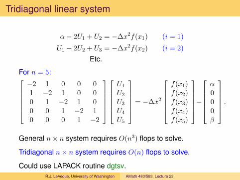
Tridiagonal linear system
α− 2U1 + U2 = −∆x2f(x1) (i = 1)
U1 − 2U2 + U3 = −∆x2f(x2) (i = 2)
Etc.
For n = 5:−2 1 0 0 01 −2 1 0 00 1 −2 1 00 0 1 −2 10 0 0 1 −2
U1
U2
U3
U4
U5
= −∆x2
f(x1)f(x2)f(x3)f(x4)f(x5)
−α000β
.
General n× n system requires O(n3) flops to solve.
Tridiagonal n× n system requires O(n) flops to solve.
Could use LAPACK routine dgtsv.
R.J. LeVeque, University of Washington AMath 483/583, Lecture 23
Tridiagonal linear system
α− 2U1 + U2 = −∆x2f(x1) (i = 1)
U1 − 2U2 + U3 = −∆x2f(x2) (i = 2)
Etc.
For n = 5:−2 1 0 0 01 −2 1 0 00 1 −2 1 00 0 1 −2 10 0 0 1 −2
U1
U2
U3
U4
U5
= −∆x2
f(x1)f(x2)f(x3)f(x4)f(x5)
−α000β
.
General n× n system requires O(n3) flops to solve.
Tridiagonal n× n system requires O(n) flops to solve.
Could use LAPACK routine dgtsv.R.J. LeVeque, University of Washington AMath 483/583, Lecture 23

Heat equation in 2 dimensions
One-dimensional equation generalizes to
ut(x, y, t) = D(uxx(x, y, t) + uyy(x, y, t)) + f(x, y, t)
on some domain in the x-y plane, with initial and boundaryconditions.
We will only consider rectangle 0 ≤ x ≤ 1, 0 ≤ y ≤ 1.
Steady state problem (with D = 1):
uxx(x, y) + uyy(x, y) = −f(x, y)
This is a PDE in two spatial variables. (Poisson Problem)
Laplace’s equation if f(x, y) ≡ 0.∇2 = (∂2
x + ∂2y) is the Laplacian operator.
R.J. LeVeque, University of Washington AMath 483/583, Lecture 23

Finite difference equations for 2D Poisson problem
Let Uij ≈ u(xi, yj).
Replace differential equation
uxx(x, y) + uyy(x, y) = −f(x, y)
by algebraic equations
1
∆x2(Ui−1,j − 2Ui,j + Ui+1,j)
+1
∆y2(Ui,j−1 − 2Ui,j + Ui,j+1) = −f(xi, yj)
If ∆x = ∆y = h:
1
h2(Ui−1,j + Ui+1,j + Ui,j−1 + Ui,j+1 − 4Ui,j) = −f(xi, yj).
R.J. LeVeque, University of Washington AMath 483/583, Lecture 23

Finite difference equations for 2D Poisson problem
1
h2(Ui−1,j + Ui+1,j + Ui,j−1 + Ui,j+1 − 4Ui,j) = −f(xi, yj).
On n× n grid (∆x = ∆y = 1/(n+ 1)) this gives a linear systemof n2 equations in n2 unknowns.
The above equation must be satisfied for i = 1, 2, . . . , n andj = 1, 2, . . . , n.
Matrix is n2 × n2,e.g. on 100 by 100 grid, matrix is 10, 000× 10, 000.
Contains (10, 000)2 = 100, 000, 000 elements.
Matrix is sparse: each row has at most 5 nonzeros out of n2
elements! But structure is no longer tridiagonal.
R.J. LeVeque, University of Washington AMath 483/583, Lecture 23

Finite difference equations for 2D Poisson problem
Matrix has block tridiagonal structure:
A =1
h2
T II T I
I T II T
T =
−4 1
1 −4 11 −4 1
1 −4
R.J. LeVeque, University of Washington AMath 483/583, Lecture 23

Iterative methods
Back to one space dimension first...
Coupled system of n linear equations:
(Ui−1 − 2Ui + Ui+1) = −∆x2f(xi)
for i = 1, 2, . . . , n. With U0 = α and Un+1 = β.
Iterative method starts with initial guess U [0] to solution andthen improves U [k] to get U [k+1] for k = 0, 1, . . ..
Note: Generally does not involve modifying matrix A.
Do not have to store matrix A at all, only know about stencil.
R.J. LeVeque, University of Washington AMath 483/583, Lecture 23

Jacobi iteration
(Ui−1 − 2Ui + Ui+1) = −∆x2f(xi)
Solve for Ui:
Ui =1
2
(Ui−1 + Ui+1 + ∆x2f(xi)
).
Note: With no heat source, f(x) = 0,the temperature at each point is average of neighbors.
Suppose U [k] is a approximation to solution. Set
U[k+1]i =
1
2
(U
[k]i−1 + U
[k]i+1 + ∆x2f(xi)
)for i = 1, 2, . . . , n.
Repeat for k = 0, 1, 2, . . . until convergence.
Can be shown to converge (eventually... very slow!)
R.J. LeVeque, University of Washington AMath 483/583, Lecture 23

Slow convergence of Jacobi
R.J. LeVeque, University of Washington AMath 483/583, Lecture 23

Slow convergence of Jacobi
R.J. LeVeque, University of Washington AMath 483/583, Lecture 23

Slow convergence of Jacobi
R.J. LeVeque, University of Washington AMath 483/583, Lecture 23

Iterative methods
Jacobi iteration is about the worst possible iterative method.
But it’s very simple, and useful as a test for parallelization.
Better iterative methods:
• Gauss-Seidel• Successive Over-Relaxation (SOR)• Conjugate gradients• Preconditioned conjugate gradients• Multigrid
R.J. LeVeque, University of Washington AMath 483/583, Lecture 23

Iterative methods – initialization
! allocate storage for boundary points too:allocate(x(0:n+1), u(0:n+1), f(0:n+1))
dx = 1.d0 / (n+1.d0)
!$omp parallel dodo i=0,n+1
! grid points:x(i) = i*dx! source term:f(i) = 100.*exp(x(i))! initial guess (linear function):u(i) = alpha + x(i)*(beta-alpha)enddo
R.J. LeVeque, University of Washington AMath 483/583, Lecture 23

Jacobi iteration in Fortran
uold = u ! starting values before updating
do iter=1,maxiter
dumax = 0.d0
do i=1,nu(i) = 0.5d0*(uold(i-1) + uold(i+1) + dx**2*f(i))dumax = max(dumax, abs(u(i)-uold(i)))enddo
! check for convergence:if (dumax .lt. tol) exit
uold = u ! for next iterationenddo
Note: we must use old value at i− 1 for Jacobi.
Otherwise we get the Gauss-Seidel method.u(i) = 0.5d0*(u(i-1) + u(i+1) + dx**2*f(i))
This actually converges faster!
R.J. LeVeque, University of Washington AMath 483/583, Lecture 23

Jacobi with OpenMP parallel do (fine grain)
See: $UWHPSC/codes/openmp/jacobi1d_omp1.f90
uold = u ! starting values before updating
do iter=1,maxiter
dumax = 0.d0
!$omp parallel do reduction(max : dumax)do i=1,nu(i) = 0.5d0*(uold(i-1) + uold(i+1) + dx**2*f(i))dumax = max(dumax, abs(u(i)-uold(i)))enddo
! check for convergence:if (dumax .lt. tol) exit
!$omp parallel dodo i=1,n
uold(i) = u(i) ! for next iterationenddo
enddo
Note: Forking threads twice each iteration.
R.J. LeVeque, University of Washington AMath 483/583, Lecture 23

Jacobi with OpenMP – coarse grain
General Approach:
• Fork threads only once at start of program.
• Each thread is responsible for some portion of the arrays,from i=istart to i=iend.
• Each iteration, must copy u to uold, update u, check forconvergence.
• Convergence check requires coordination between threadsto get global dumax.
• Print out final result after leaving parallel block
See code in the repository or the notes:$UWHPSC/codes/openmp/jacobi1d_omp2.f90
R.J. LeVeque, University of Washington AMath 483/583, Lecture 23
Related Documents