ALU Organization Michael Vong Louis Young Rongli Zhu Dan.

ALU Organization

Michael VongLouis YoungRongli Zhu

Dan

Overall ALU Organization

• The output lines (Y3 … Y0) run all the way through

ALU Organization:One Function Per Column

Control signals will enable all transmission gates in a column

ALU Organization:One Bit Per Row

Only one transmission gate in a row will be turned on. Only one function will drive Y.

Adder Logic Design

BK Cell States

• Our adder uses BK Cells.

• For each column of addition, there are three possible states.

0 1 0

+ 1 1 0

(0 + 1) or (1 + 0) is carry propagate = P

(1 + 1) is carry generate = G

(0 + 0) is carry kill = K

BK Cell Truth Table

More Significant Input Less Significant Input Output

K K K

K P K

K G K

P K K

P P P

P G G

G K G

G P G

G G G

Each BK cell looks at the carry status of two networks and generate a single carry status.

BK Cell Boolean Equation• Y1 = BD + AD + AB

• Y0 = BC + AC + ABNote:

•The encoding used: G = 11, K = 00, and P = 10 or 01

• Y1 and Y0 are the same Boolean function. Just do the layout for Y1 and replicate it twice to get a BK cell

•This is the same function as the ripple adder’s carry out

Using BK Cells to make an Adder

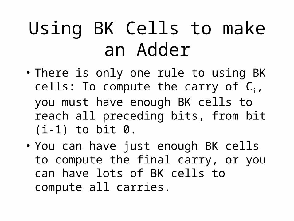
• There is only one rule to using BK cells: To compute the carry of Ci, you must have enough BK cells to reach all preceding bits, from bit (i-1) to bit 0.

• You can have just enough BK cells to compute the final carry, or you can have lots of BK cells to compute all carries.

BK Cell Example(part 1 of 2)

If you just want the carry out of an 8 bit addition operation, then you will need 7 BK cells.

BK Cell Example(part 2 of 2)

• Note that the first input into the first BK cell on the right (the C and D of the red box), must be either G (11) or K (00). Let say the number we are adding are called A and B, this input is C = D = A0Bin + A0Cin + B0Cin .

• The final output, the Y1 and Y0 of the yellow box, is also either G(11) or K(00).

Our Adder’s BK Cells

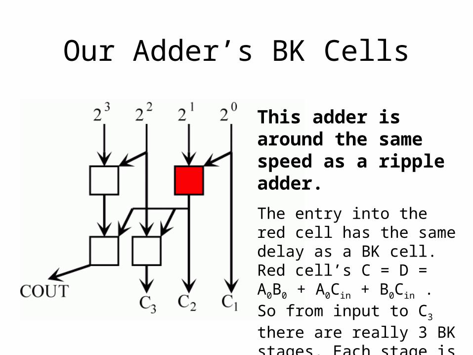
This adder is around the same speed as a ripple adder.

The entry into the red cell has the same delay as a BK cell. Red cell’s C = D = A0B0 + A0Cin + B0Cin . So from input to C3 there are really 3 BK stages. Each stage is the same as a carry out of a ripple.

Other BK Cell Examples

Our adder does not benefit from the BK cells because it’s only 4 bits wide. Larger adders do benefit.

Screen shots are taken from:

http://tima-cmp.imag.fr/~guyot/Cours/Oparithm/english/Additi.htm

Sklanski's adder:

Problem: high fan-out for the lowest C8 BK cell.

Another BK Cell ExampleKogge & Stone adders:

This one has more BK cells but less fan-out.

Our Adder --- After the BK Tree

• After the carries are generated, add them to the xor sums.• If we are add A and B, and let the answer be SUM:

SUM0 = (A0 xor B0) xor C0

SUM1 = (A1 xor B1) xor C1

SUM2 = (A2 xor B2) xor C2

SUM3 = (A3 xor B3) xor C3

This operation of two xor gates is called the “summer” in our adder.

Summer Schematic

The idea is to have A and B preset a path so that when C is correctly set, it will show up at Y really fast. It didn’t work out that well.

Y = (A XOR B) XOR C

Adder Logic Summary

• A tree of BK cells are used to compute all of the carries.

• The final sum for the i-th bit is Ai xor Bi xor Ci , where A and B are the numbers that we are adding, and C is the carry computed by the BK cells.

Confirming the Logic with Verilog

module bk(Y1, Y0, A, B, C, D); input A, B, C, D; output Y1, Y0; assign Y1 = (B&D) | (A&D) | (A&B); assign Y0 = (B&C) | (A&C) | (A&B);endmodule

module summer(Y, A, B, C); input A, B, C; output Y; assign Y = (~A & ~B & C) | (~A & B & ~C) | (A & ~B & ~C) | (A & B & C);

endmodule

adder.v (page 1)module adder(SUM, COUT, A, B, CIN);

input [3:0] A, B;

input CIN;

output [3:0] SUM;

output COUT;

wire c1, c2, c3, c4;

assign c1 = (A[0] & B[0]) | (A[0] & CIN) | (B[0] & CIN);

wire bk1_0, bk1_1, bk2_0, bk2_1;

wire bk3_0, bk3_1, bk4_0, bk_1;

bk bk1(bk1_1, bk1_0, A[1], B[1], c1, c1);

bk bk2(bk2_1, bk2_0, A[2], B[2], bk1_1, bk1_0);

bk bk3(bk3_1, bk3_0, A[3], B[3], A[2], B[2]);

bk bk4(bk4_1, bk4_0, bk3_1, bk3_0, bk1_1, bk1_0);

adder.v (page 2)assign c4 = bk4_1;

assign c3 = bk2_1;

assign c2 = bk1_1;

assign COUT = c4;

summer s0(SUM[0], A[0], B[0], CIN);

summer s1(SUM[1], A[1], B[1], c1);

summer s2(SUM[2], A[2], B[2], c2);

summer s3(SUM[3], A[3], B[3], c3);

endmodule

test.vmodule testbench;

wire [3:0] SUM;wire COUT;reg [3:0] A, B;reg CIN;

adder adder1(SUM, COUT, A, B, CIN);

reg [4:0] i, j, k;

initial begin

CIN = 4'd1; for(i = 0; i < 16; i = i + 1)

beginfor(j = 0; j < 16; j = j + 1)begin

A[3:0] = i[3:0];B[3:0] = j[3:0];#20;

k = i + j + 1;

test.v (page 2)

if(SUM[3:0] != k[3:0])begin$display("At time %t, A = %d, B = %d, CIN

= %d, SUM = %d, COUT = %d \n", $time, A, B, CIN, SUM, COUT);

endelsebegin$display("A = %d, B = %d, CIN = %d

tested \n", A, B, CIN);end

endend$display("end of test \n");

end

endmodule

Simulation with ModelSim

Adder Circuitry

Layout Guidelines

PMOS: L = 0.6 um, W = 5.4 um

NMOS: L = 0.6 um, W = 3 um

Transistor Sizes (most of the time):

Cell height:

Total Height: 27 um

VDD and GND path width: 1.5 um

Cell Hierarchy

• zproj_adder4b– zproj_bk

• zproj_bk_y1

– zproj_summer• Zproj_mux2b

The bk_y1 Cell AOI Schematic

Recall that the BK cell has a Y1 and Y0

The bk_y1 layout

Note that metal 2 can route vertically through almost all of the cell.

The Complete BK Cell Schematic

The bk Cell Layout View 1

The bk Cell Layout View 2A and B is the same all the way across while C and D swap

rows

Y1 is in the middle while Y0 is at the far right

Multiplexer Schematic

The multiplexer is the basic cell for the summer

Multiplexer Schematic

Multiplexer Layout

Note that vertical routing of metal 2 is possible in less than half of the cell.

Multiplexer Test Setup

Note how ideal sources are fed directly into the mux

Multiplexer Power Usage

Multiplexer Test ResultThe load capacitance is 30 fF

S ONE ZERO Y Time (ns)

5 5->0 5->0 0.0757 ??

5 0->5 0->5 0.08765 ??

0 0->5 0->5 0.0747 ??

0 5->0 5->0 0.0832 ??

0->5 5 0 0->5 0.181

0->5 0 5 5->0 0.144

5->0 5 0 5->0 0.176

5->0 0 5 0->5 0.133

Multiplexer Test Results (Page 2)

Power = 14.95 W/cm2

The first group of results highlighted in red cells turned out to be inaccurate. The ONE and ZERO lines are not gate terminals. When the path way is set (S held steady), the rate at which the output changes is actually proportional to the change in input. The output is changing rapidly in the test because the input is an ideal voltage source with a rise time of 200 ps.

A more realistic switching time can be obtained by passing the ideal input through two inverters before sending it to the “ONE” or “ZERO” line of the multiplexer.

Summer Schematic

Summer Layout View 1

The (NOT C) is labeled as C’

Summer Layout View 2

The right most Y is the sum

Putting the Support Cells Together to Form a 4 Bit Adder

Adder Schematic Page 1This is the BK tree part of the adder

Adder Schematic Page 2

Output from the BK tree, and the original A and B bits are passed into the summer cells.

Adder Layout Adder Layout

Note the long distance metal2 vertical routing

Adder Layout View 2

Adder LayoutInput View

Adder Layout Output

View

Adder Layout Area

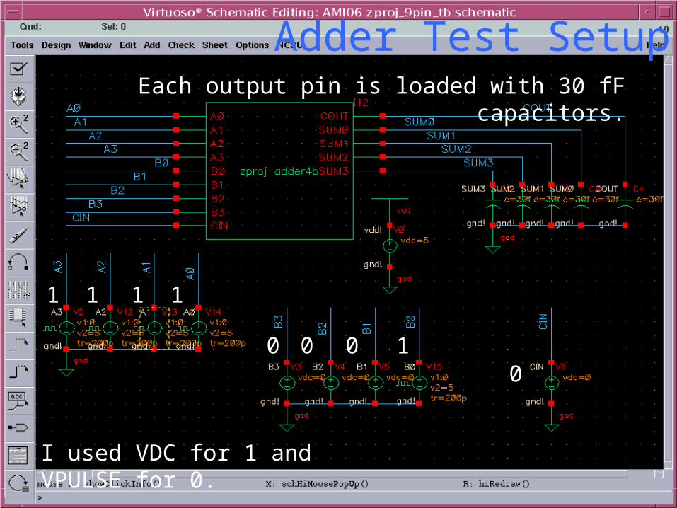
Adder Test Setup

I used VDC for 1 and VPULSE for 0.

1 1 1 1

100 00

Each output pin is loaded with 30 fF capacitors.

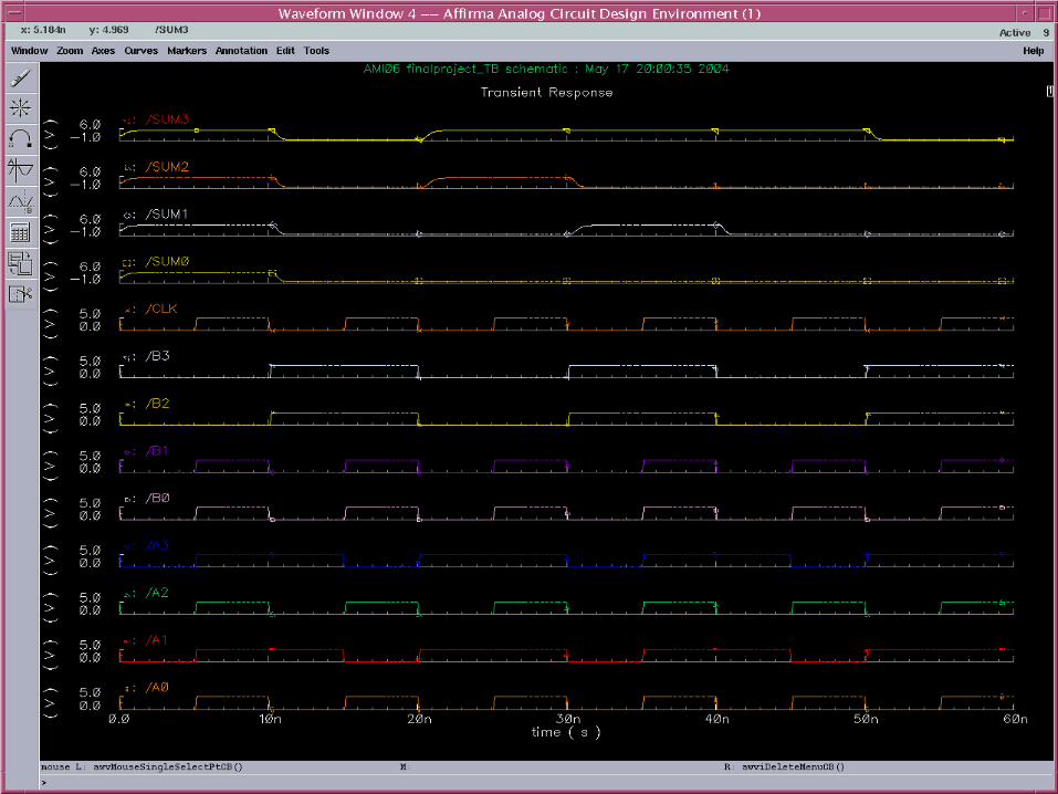
Adder Testing Results

A B CIN COUT > 2.5v

SUM3 < 2.5V

SUM3 < 1V

1111 0001 0 2.534 ns 3.264 ns 4.192 ns

1111 0000 1 2.39 ns 3.111 ns 4.039 ns

0001 1111 0 2.133 ns 2.33 ns 3.150 ns

0000 1111 1 1.785 ns 1.906 ns 2.726 ns

1011 0101 1 1.988 ns 2.22 ns 3.069 ns

Adder Worst Case

• A = 1111• B = 0001• CIN = 0

Note the sagging SUM3 output.

SUM 3 output is sagging because it is 4 Transistor

Away from GND

Speeding up SUM3’s Rate of Change with a Multiplexer

The capacitor now charges and discharges faster because it is closer to VDD and GND. However, the multiplexer will be an extra delay

Effect of using an extra multiplexer at the output:

-Y_fast will arrive at 2.5V 0.35 ns later.

-Y_fast will arrive at 1V 0.324 ns earlier.

Timing without a Multiplexer Buffer

SUM3 is changes slowly if its output is used to charge 30fF of capacitance directly.

Note the time scale for this test goes up to 16 ns.

Timing with a Multiplexer Buffer

Note the time scale for this test goes up to just 12 ns.

Passing SUM3’s output to a multiplexer buffer delays the wave but increase the rate of change.

ALU Schematic

DRC of ALU

Extracted View

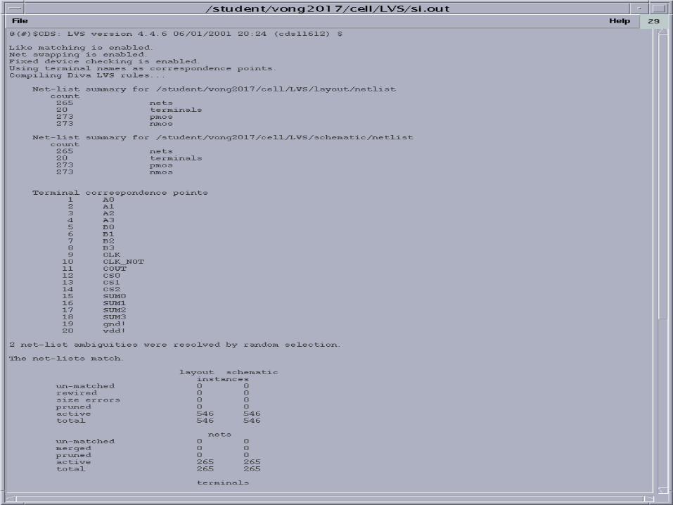
LVS